chapter 7 exploring variation: functional principal and...

Chapter 7Exploring Variation: Functional Principal andCanonical Components Analysis

Now we look at how observations vary from one replication or sampled value to thenext. There is, of course, also variation within observations, but we focused on thattype of variation when considering data smoothing in Chapter 5.

Principal components analysis, or PCA, is often the first method that we turn toafter descriptive statistics and plots. We want to see what primary modes of varia-tion are in the data, and how many of them seem to be substantial. As in multivariatestatistics, eigenvalues of the bivariate variance-covariance function v(s, t) are indi-cators of the importance of these principal components, and plotting eigenvalues isa method for determining how many principal components are required to producea reasonable summary of the data.

In functional PCA, there is an eigenfunction associated with each eigenvalue,rather than an eigenvector. These eigenfunctions describe major variational compo-nents. Applying a rotation to them often results in a more interpretable picture ofthe dominant modes of variation in the functional data, without changing the totalamount of common variation.

We take some time over PCA partly because this may be the most common func-tional data analysis and because the tasks that we face in PCA and our approaches tothem will also be found in more model-oriented tools such as functional regressionanalysis. For example, we will see that each eigenfunction can be constrained tobe smooth by the use of roughness penalties, just as in the data smoothing process.Should we use rough functions to capture every last bit of interesting variation in thedata and then force the eigenfunctions to be smooth, or should we carefully smooththe data first before doing PCA?

A companion problem is the analysis of the covariation between two differentfunctional variables based on samples taken from the same set of cases or individu-als. For example, what types of variation over weather stations do temperature andlog precipitation share? How do knee and hip angles covary over the gait cycle?Canonical correlation analysis (CCA) is the method of choice here. We will seemany similarities between PCA and CCA.

J. Ramsay et al., Functional Data Analysis with R and MATLAB, Use R,

© Springer Science + Business Media, LLC 2009

99DOI: 10.1007/978-0-387-98185-7_7,

O.

100 7 Exploring Variation: Functional Principal and Canonical Components Analysis

7.1 An Overview of Functional PCA

In multivariate statistics, variation is usually summarized by either the covariancematrix or the correlation matrix. Because the variables in a multivariate observationcan vary a great deal in location and scale due to relatively arbitrary choices oforigin and unit of measurement, and because location/scale variation tends to beuninteresting, multivariate analyses are usually based on the correlation matrix. Butwhen an observation is functional, values xi(s) and xi(t) have the same origin andscale. Consequently, either the estimated covariance function

v(s, t) = (N−1)−1 ∑i[xi(s)− x(s)][xi(t)− x(t)],

or the cross-product function

c(s, t) = N−1 ∑i

xi(s)xi(t),

will tend to be more useful than the correlation function

r(s, t) =v(s, t)√

[v(s,s)v(t, t)].

Principal components analysis may be defined in many ways, but its motivationis perhaps clearer if we define PCA as the search for a probe ξ , of the kind that wedefined in Chapter 6, that reveals the most important type of variation in the data.That is, we ask, “For what weight function ξ would the probe scores

ρξ (xi) =∫

ξ (t)xi(t)dt

have the largest possible variation?” In order for the question to make sense, wehave to impose a size restriction on ξ , and it is mathematically natural to requirethat

∫ξ 2(t)dt = 1.

Of course, the mean curve by definition is a mode of variation that tends to beshared by most curves, and we already know how to estimate this. Consequently, weusually remove the mean first and then probe the functional residuals xi− x. Later,when we look at various types of functional regression, we may also want to firstremove other known sources of variation that are explainable by multivariate and/orfunctional covariates.

The probe score variance Var[∫

ξ (t)(xi(t)− x(t))2dt] associated with a probeweight ξ is the value of

µ = maxξ{∑

iρ2

ξ (xi)} subject to∫

ξ 2(t)dt = 1. (7.1)

7.1 An Overview of Functional PCA 101

In standard terminology, µ and ξ are referred to as the largest eigenvalue and eigen-function, respectively, of the estimated variance-covariance function v. An alterna-tive to the slightly intimidating term “eigenfunction” is harmonic.

As in multivariate PCA, a nonincreasing sequence of eigenvalues µ1 ≥ µ2 ≥. . .µk can be constructed stepwise by requiring each new eigenfunction, computedin step `, to be orthogonal to those computed on previous steps,

∫ξ j(t)ξ`(t)dt = 0, j = 1, . . . , `−1 and

∫ξ 2` (t)dt = 1. (7.2)

In multivariate settings the entire suite of eigenvalue/eigenvector pairs would becomputed by the eigenanalysis of the covariance matrix V, solving the matrix eigen-equation Vξ j = µ jξ j. The approach is essentially the same for functional data;that is, we calculate eigenfunctions ξ j of the bivariate covariance function v(s, t) assolutions of the functional eigenequation

∫v(s, t)ξ j(t)dt = µ jξ j(s). (7.3)

We see here as well as elsewhere that going from multivariate to functional dataanalysis is often only a matter of replacing summation over integer indices by inte-gration over continuous indices such as t. Although the computation details are notat all the same, this is thankfully hidden by the notation and dealt with in the fdapackage.

However, there is an important difference between multivariate and functionalPCA caused by the fact that, whereas in multivariate data the number of variables pis usually less than the number of observations N, for functional data the number ofobserved function values n is usually greater than N. This implies that the maximumnumber of nonzero eigenvalues in the functional context is min{N−1,K,n}, and inmost applications will be N−1.

Suppose, then, that our software can present us with, say, N− 1 positive eigen-value/eigenfunction pairs (µ j,ξ j). What do we do next? For each choice of `,1 ≤ ` ≤ N − 1, the ` leading eigenfunctions or harmonics define a basis systemthat can be used to approximate the sample functions xi. These basis functions areorthogonal to each other and are normalized in the sense that

∫ξ 2

` = 1. They aretherefore referred to as an orthonormal basis. They are also the most efficient basispossible of size ` in the sense that the total error sum of squares

PCASSE=N

∑i

∫[xi(t)− x(t)− c′iξ (t)]2dt (7.4)

is the minimum achievable with only ` basis functions. Of course, other `-dimensionalsystems certainly exist that will do as well, and we will consider some shortly, butnone will do better. In the physical sciences, these optimal basis functions ξ j areoften referred to as empirical orthogonal functions.

It turns out that there is a simple relationship between the optimal total squarederror and the eigenvalues that are discarded, namely that


PCASSE=N−1

∑j=`+1

µ j.

It is usual, therefore, to base a decision on the number ` of harmonics to use on avisual inspection of a plot of the eigenvalues µ j against their indices j, a displaythat is often referred to in the social science literature as a scree plot. Although thereare a number of proposals for automatic data-based rules for deciding the value of`, many nonstatistical considerations can also affect this choice.

The coefficient vectors ci, i = 1, . . . ,N contain the coefficients ci j that define theoptimal fit to each function xi, and are referred to as principal component scores.They are given by the following:

ci j = ρξ j(xi− x) =∫

ξ j(t)[xi(t)− x(t)]dt. (7.5)

As we will show below, they can be quite helpful in interpreting the nature of thevariation identified by the PCA. It is also common practice to treat these scores as“data” to be subjected to a more conventional multivariate analysis.

We suggested that the eigenfunction basis was optimal but not unique. In fact, forany nonsingular square matrix L of order `, the system φ = Tξ is also optimal andspans exactly the same functional subspace as that spanned by the eigenfunctions.Moreover, if T′ = T−1, such matrices being often referred to as rotation matrices,the new system φ is also orthonormal. There is, in short, no mystical significance tothe eigenfunctions that PCA generates, a simple fact that is often overlooked in text-books on multivariate statistics. Well, okay, perhaps ` = 1 is an exception. In fact,it tends to happen that only the leading eigenfunction has an obvious meaningfulinterpretation in terms of processes known to generate the data.

But for ` > 1, there is nothing to prevent us from searching among the infinitenumber of alternative systems φ = Tξ to find one where all of the orthonormal basisfunctions φ j are seen to have some substantive interpretation. In the social sciences,where this practice is routine, a number of criteria for optimizing the chances ofinterpretability have been devised for choosing a rotation matrix T, and we willdemonstrate the usefulness of the popular VARIMAX criterion in our examples.

Readers are referred at this point to standard texts on multivariate data analysisor to the more specialized treatment in Jolliffe (2002) for further information onprincipal components analysis. Most of the material in these sources applies to thisfunctional context.

7.2 PCA with Function pca.fd

Principal component analysis is implemented in the functions pca.fd and pca fdin R and Matlab, respectively. The call in R is

pca.fd(fdobj, nharm = 2, harmfdPar=fdPar(fdobj),

7.2 PCA with Function pca.fd 103

centerfns = TRUE)

The first argument is a functional data object containing the functional data to beanalyzed, and the second specifies the number ` of principal components to be re-tained. The third argument is a functional parameter object that provides the in-formation necessary to smooth the eigenfunctions if necessary; we will postponethis topic to Section 7.3. Finally, although most principal components analyses areapplied to data with the mean function subtracted from each function, the final ar-gument permits this to be suppressed.

Function pca.fd in R returns an object with the class name pca.fd, so that itis effectively a constructor function. Here are the named components for this class:

harmonics A functional data object for the ` harmonics or eigenfunctions ξ j.values The complete set of eigenvalues µ j.scores The matrix of scores ci j on the principal components or harmonics.varprop A vector giving the proportion µ j/∑ µ j of variance explained by each

eigenfunction.meanfd A functional data object giving the mean function x.

7.2.1 PCA of the Log Precipitation Data

Here is the command to do a PCA using only two principal components for the logprecipitation data and to display the eigenvalues.

logprec.pcalist = pca.fd(logprecfd, 2)print(logprec.pcalist$values)

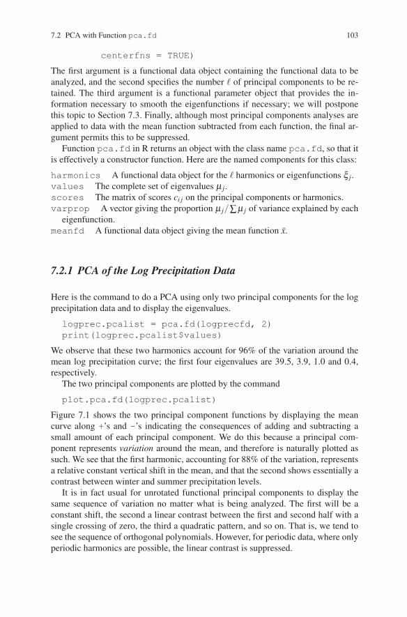
We observe that these two harmonics account for 96% of the variation around themean log precipitation curve; the first four eigenvalues are 39.5, 3.9, 1.0 and 0.4,respectively.

The two principal components are plotted by the command

plot.pca.fd(logprec.pcalist)

Figure 7.1 shows the two principal component functions by displaying the meancurve along +’s and -’s indicating the consequences of adding and subtracting asmall amount of each principal component. We do this because a principal com-ponent represents variation around the mean, and therefore is naturally plotted assuch. We see that the first harmonic, accounting for 88% of the variation, representsa relative constant vertical shift in the mean, and that the second shows essentially acontrast between winter and summer precipitation levels.

It is in fact usual for unrotated functional principal components to display thesame sequence of variation no matter what is being analyzed. The first will be aconstant shift, the second a linear contrast between the first and second half with asingle crossing of zero, the third a quadratic pattern, and so on. That is, we tend tosee the sequence of orthogonal polynomials. However, for periodic data, where onlyperiodic harmonics are possible, the linear contrast is suppressed.


0 100 200 3000.

000.

100.

200.

30

PCA function 1 (Percentage of variability 87.4 )

Har

mon

ic 1

+++++++++++++++++++++++++++++++++++++++++++++++++++++++++++++++++++++++++++++++++++++++++++++++++++++

+++++++

+++++++++++++

+++++++−−−−−−−−−−−−−−−−−−

−−−−−−−−−−−−−−−−−−−−−−−−−−−−−−−−−−−−−−−−−−−−−−−−−−−−−−−−−−−−−−−−−−−−−−−−−−−−−−−−−−−−−

−−−−−−−−−−−−−−−−−−−−

−−−−−

0 100 200 300

0.05

0.15

0.25


Har

mon

ic 2

+++++++++++++++++++++++++++++++++++++++++++++++++++++++++++++++++++++++++++++++++++++++++++++++++++

+++++++

+++++++++++++++++

+++++

−−−−−−−−−−−−−−−−−

−−−−−−−−−−−−−−−−−−−−−−−−−−−−−−−−−−−−−−−−−−−−−−−−−−−−−−−−−−−−−−−−−−−−−−−−−−−−−−−−−−−−−−−−−−

−−−−−−−−−−−−−−

−−−−−−−

Fig. 7.1 The two principal component functions or harmonics are shown as perturbations of themean, which is the solid line. The +’s show what happens when a small amount of a principalcomponent is added to the mean, and the -’s show the effect of subtracting the component.

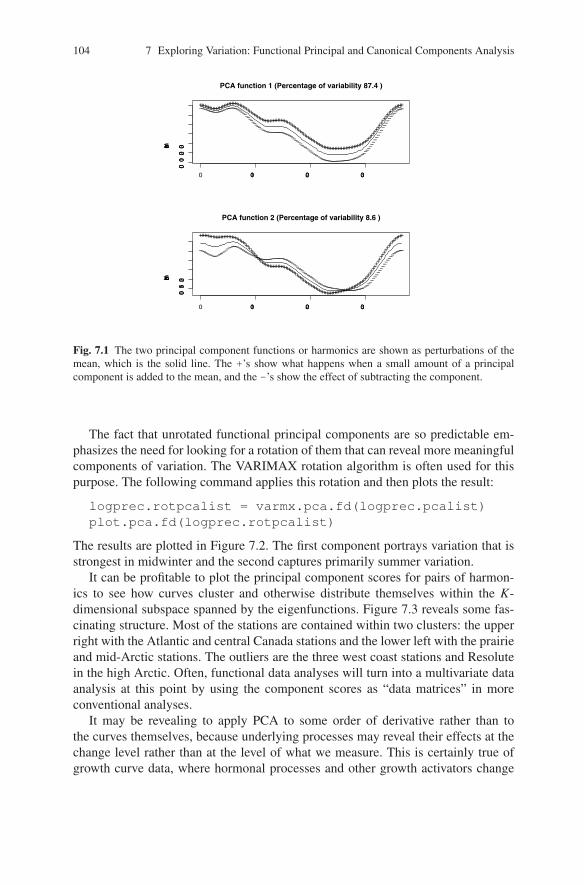
The fact that unrotated functional principal components are so predictable em-phasizes the need for looking for a rotation of them that can reveal more meaningfulcomponents of variation. The VARIMAX rotation algorithm is often used for thispurpose. The following command applies this rotation and then plots the result:

logprec.rotpcalist = varmx.pca.fd(logprec.pcalist)plot.pca.fd(logprec.rotpcalist)

The results are plotted in Figure 7.2. The first component portrays variation that isstrongest in midwinter and the second captures primarily summer variation.

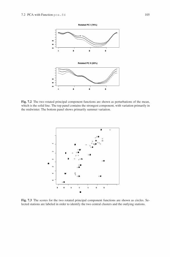
It can be profitable to plot the principal component scores for pairs of harmon-ics to see how curves cluster and otherwise distribute themselves within the K-dimensional subspace spanned by the eigenfunctions. Figure 7.3 reveals some fas-cinating structure. Most of the stations are contained within two clusters: the upperright with the Atlantic and central Canada stations and the lower left with the prairieand mid-Arctic stations. The outliers are the three west coast stations and Resolutein the high Arctic. Often, functional data analyses will turn into a multivariate dataanalysis at this point by using the component scores as “data matrices” in moreconventional analyses.

It may be revealing to apply PCA to some order of derivative rather than tothe curves themselves, because underlying processes may reveal their effects at thechange level rather than at the level of what we measure. This is certainly true ofgrowth curve data, where hormonal processes and other growth activators change

7.2 PCA with Function pca.fd 105

0 100 200 3000.

000.

150.

30

Rotated PC I (76%)

++++++++++++++++++++++++++++++++++++++++++++++++++++++++++++++++++++++++++−−−−−−−−−−−−−−−−−−−−−−−−−−−−−−−−−−−−−−−−−−−−−−−−−−−−−−−−−−−−−−−−−−−−−−−−−−

0 100 200 300

0.00

0.15

0.30

Rotated PC II (20%)

++++++++++++++++++++++++++++++++++++++++++++++++++++++++++++++++++++++++++

−−−−−−−−−−−−−−−−−−−−−−−−−−−−−−−−−−−−−−−−−−−−−−−−−−−−−−−−−−−−−−−−−−−−−−−−−−

Fig. 7.2 The two rotated principal component functions are shown as perturbations of the mean,which is the solid line. The top panel contains the strongest component, with variation primarily inthe midwinter. The bottom panel shows primarily summer variation.

−15 −10 −5 0 5 10 15

−6

−4

−2

02

4

Rotated Harmonic I

Rot

ated

Har

mon

ic II

Quebec

Montreal

TorontoWinnipeg

Uranium Cty

Edmonton

Kamloops

Vancouver

Victoria

Pr. George

Dawson

Iqaluit

Resolute

Halifax

Thunder Bay

Regina

Calgary

Pr. Rupert

Whitehorse

Fig. 7.3 The scores for the two rotated principal component functions are shown as circles. Se-lected stations are labeled in order to identify the two central clusters and the outlying stations.


the rate of change of height and can be especially evident at the level of the acceler-ation curves that we plotted in Section 1.1.

7.2.2 PCA of Log Precipitation Residuals

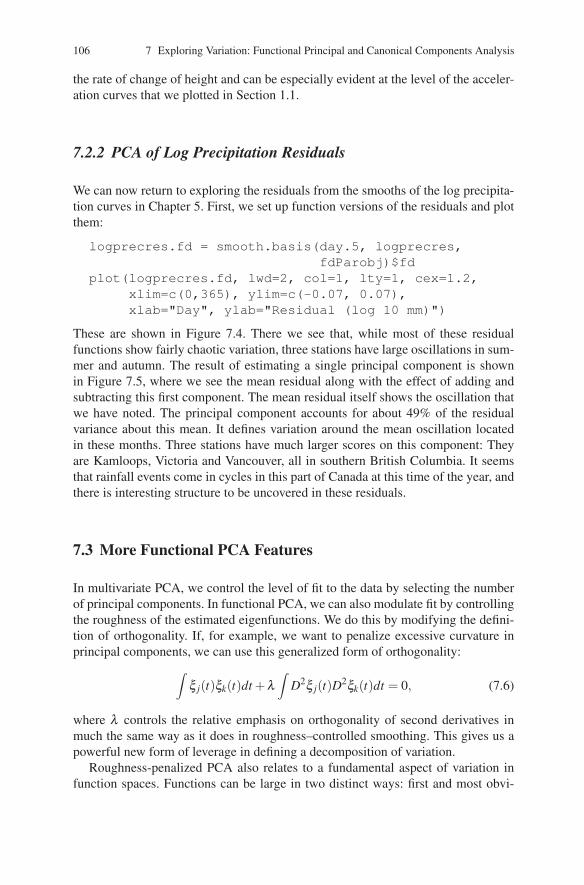
We can now return to exploring the residuals from the smooths of the log precipita-tion curves in Chapter 5. First, we set up function versions of the residuals and plotthem:

logprecres.fd = smooth.basis(day.5, logprecres,fdParobj)$fd

plot(logprecres.fd, lwd=2, col=1, lty=1, cex=1.2,xlim=c(0,365), ylim=c(-0.07, 0.07),xlab="Day", ylab="Residual (log 10 mm)")

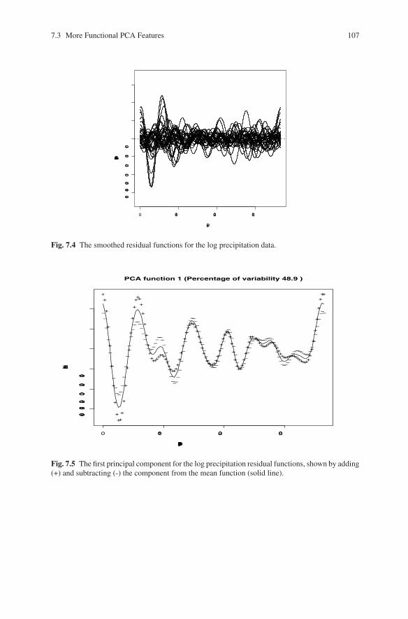
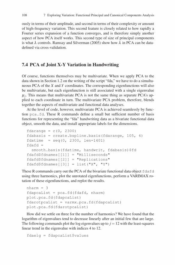
These are shown in Figure 7.4. There we see that, while most of these residualfunctions show fairly chaotic variation, three stations have large oscillations in sum-mer and autumn. The result of estimating a single principal component is shownin Figure 7.5, where we see the mean residual along with the effect of adding andsubtracting this first component. The mean residual itself shows the oscillation thatwe have noted. The principal component accounts for about 49% of the residualvariance about this mean. It defines variation around the mean oscillation locatedin these months. Three stations have much larger scores on this component: Theyare Kamloops, Victoria and Vancouver, all in southern British Columbia. It seemsthat rainfall events come in cycles in this part of Canada at this time of the year, andthere is interesting structure to be uncovered in these residuals.

7.3 More Functional PCA Features

In multivariate PCA, we control the level of fit to the data by selecting the numberof principal components. In functional PCA, we can also modulate fit by controllingthe roughness of the estimated eigenfunctions. We do this by modifying the defini-tion of orthogonality. If, for example, we want to penalize excessive curvature inprincipal components, we can use this generalized form of orthogonality:

∫ξ j(t)ξk(t)dt +λ

∫D2ξ j(t)D2ξk(t)dt = 0, (7.6)

where λ controls the relative emphasis on orthogonality of second derivatives inmuch the same way as it does in roughness–controlled smoothing. This gives us apowerful new form of leverage in defining a decomposition of variation.

Roughness-penalized PCA also relates to a fundamental aspect of variation infunction spaces. Functions can be large in two distinct ways: first and most obvi-

7.3 More Functional PCA Features 107

0 100 200 300

−0.

06−

0.04

−0.

020.

000.

020.

040.

06

Day

Res

idua

l (lo

g 10

mm

)

Fig. 7.4 The smoothed residual functions for the log precipitation data.

0 100 200 300

−0.00

6−0

.004

−0.00

20.0

000.0

020.0

04


Day (July 1 to June 30)

Harm

onic

1

++

+

+

+

+

+

+

+++

+

+

+

+

+

+

+

+

++++

+

+

+

+

+++++

+++++++++++

++

+

+

++++++

++++++++++++

+++++++++

+

+

++++++

++++++++++++++

++++++++++++++++++++++

+++

+

+

+

+

+++

−−

−

−

−

−

−

−−−−−

−

−

−

−

−

−−−−−

−−−−−−−

−−−−−−

−

−

−

−

−−−−

−

−

−

−

−

−

−−−−−

−−

−

−−−−−−−−−

−−

−

−−−−−

−

−

−

−−−−

−−−−−−−−−−−−−−

−−−−−−−−−−−

−−−−−−−−−−−−−

−−−

−

−

−−−−

Fig. 7.5 The first principal component for the log precipitation residual functions, shown by adding(+) and subtracting (-) the component from the mean function (solid line).


ously in terms of their amplitude, and second in terms of their complexity or amountof high-frequency variation. This second feature is closely related to how rapidly aFourier series expansion of a function converges, and is therefore simply anotheraspect of how PCA itself works. This second type of size of principal componentsis what λ controls. Ramsay and Silverman (2005) show how λ in PCA can be data-defined via cross-validation.

7.4 PCA of Joint X-Y Variation in Handwriting

Of course, functions themselves may be multivariate. When we apply PCA to thedata shown in Section 1.2 on the writing of the script “fda,” we have to do a simulta-neous PCA of the X and Y coordinates. The corresponding eigenfunctions will alsobe multivariate, but each eigenfunction is still associated with a single eigenvalueµ j. This means that multivariate PCA is not the same thing as separate PCA’s ap-plied to each coordinate in turn. The multivariate PCA problem, therefore, blendstogether the aspects of multivariate and functional data analyses.

At the level of code, however, multivariate PCA is achieved seamlessly by func-tion pca.fd. These R commands define a small but sufficient number of basisfunctions for representing the “fda” handwriting data as a bivariate functional dataobject, smooth the data, and install appropriate labels for the dimensions.

fdarange = c(0, 2300)fdabasis = create.bspline.basis(fdarange, 105, 6)fdatime = seq(0, 2300, len=1401)fdafd =smooth.basis(fdatime, handwrit, fdabasis)$fd

fdafd$fdnames[[1]] = "Milliseconds"fdafd$fdnames[[2]] = "Replications"fdafd$fdnames[[3]] = list("X", "Y")

These R commands carry out the PCA of the bivariate functional data object fdafdusing three harmonics, plot the unrotated eigenfunctions, perform a VARIMAX ro-tation of these eigenfunctions, and replot the results.

nharm = 3fdapcaList = pca.fd(fdafd, nharm)plot.pca.fd(fdapcaList)fdarotpcaList = varmx.pca.fd(fdapcaList)plot.pca.fd(fdarotpcaList)

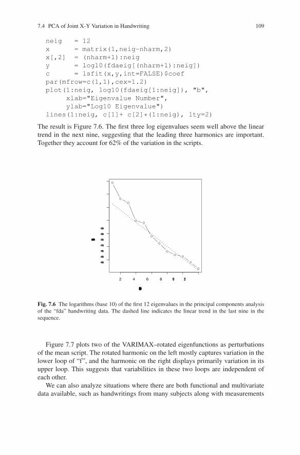
How did we settle on three for the number of harmonics? We have found that thelogarithm of eigenvalues tend to decrease linearly after an initial few that are large.The following commands plot the log eigenvalues up to j = 12 with the least-squareslinear trend in the eigenvalue with indices 4 to 12.

fdaeig = fdapcaList$values

7.4 PCA of Joint X-Y Variation in Handwriting 109

neig = 12x = matrix(1,neig-nharm,2)x[,2] = (nharm+1):neigy = log10(fdaeig[(nharm+1):neig])c = lsfit(x,y,int=FALSE)$coefpar(mfrow=c(1,1),cex=1.2)plot(1:neig, log10(fdaeig[1:neig]), "b",

xlab="Eigenvalue Number",ylab="Log10 Eigenvalue")

lines(1:neig, c[1]+ c[2]*(1:neig), lty=2)

The result is Figure 7.6. The first three log eigenvalues seem well above the lineartrend in the next nine, suggesting that the leading three harmonics are important.Together they account for 62% of the variation in the scripts.

2 4 6 8 10 12

−3.

8−

3.6

−3.

4−

3.2

−3.

0−

2.8

−2.

6

Eigenvalue Number

Log1

0 E

igen

valu

e

Fig. 7.6 The logarithms (base 10) of the first 12 eigenvalues in the principal components analysisof the “fda” handwriting data. The dashed line indicates the linear trend in the last nine in thesequence.

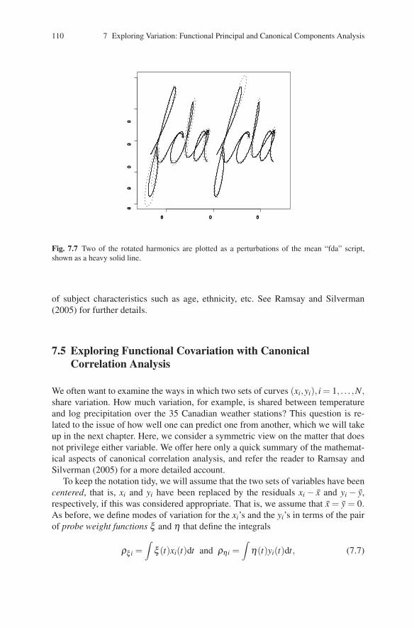
Figure 7.7 plots two of the VARIMAX–rotated eigenfunctions as perturbationsof the mean script. The rotated harmonic on the left mostly captures variation in thelower loop of “f”, and the harmonic on the right displays primarily variation in itsupper loop. This suggests that variabilities in these two loops are independent ofeach other.

We can also analyze situations where there are both functional and multivariatedata available, such as handwritings from many subjects along with measurements


−0.05 0.00 0.05

−0.

04−

0.02

0.00

0.02

0.04

Fig. 7.7 Two of the rotated harmonics are plotted as a perturbations of the mean “fda” script,shown as a heavy solid line.

of subject characteristics such as age, ethnicity, etc. See Ramsay and Silverman(2005) for further details.

7.5 Exploring Functional Covariation with CanonicalCorrelation Analysis

We often want to examine the ways in which two sets of curves (xi,yi), i = 1, . . . ,N,share variation. How much variation, for example, is shared between temperatureand log precipitation over the 35 Canadian weather stations? This question is re-lated to the issue of how well one can predict one from another, which we will takeup in the next chapter. Here, we consider a symmetric view on the matter that doesnot privilege either variable. We offer here only a quick summary of the mathemat-ical aspects of canonical correlation analysis, and refer the reader to Ramsay andSilverman (2005) for a more detailed account.

To keep the notation tidy, we will assume that the two sets of variables have beencentered, that is, xi and yi have been replaced by the residuals xi − x and yi − y,respectively, if this was considered appropriate. That is, we assume that x = y = 0.As before, we define modes of variation for the xi’s and the yi’s in terms of the pairof probe weight functions ξ and η that define the integrals

ρξ i =∫

ξ (t)xi(t)dt and ρη i =∫

η(t)yi(t)dt, (7.7)

7.5 Exploring Functional Covariation with Canonical Correlation Analysis 111

respectively. The N pairs of probe scores (ρξ i,ρη i) defined in this way representshared variation if they correlate strongly with one another.

The canonical correlation criterion is the squared correlation

R2(ξ ,η) =[∑i ρξ iρη i]2

[∑i ρ2ξ i][∑i ρ2

η i]=

[∑i(∫

ξ (t)xi(t)dt)(∫

η(t)yi(t)dt)]2

[∑i(∫

ξ (t)xi(t)dt)2][∑i(∫

η(t)yi(t)dt)2]. (7.8)

As in PCA, the probe weights ξ and η are then specified by finding that weightpair that optimizes the criterion R2(ξ ,η). But, again as in PCA, we can compute anonincreasing series of squared canonical correlations R2

1,R22, . . . ,R

2k by constraining

successive canonical probe values to be orthogonal. The length k of the sequence isthe smallest of the sample size N, the number of basis functions for either functionalvariable, or the number of basis functions used for ξ and η .

That we are now optimizing with respect to two probes at the same time makescanonical correlation analysis an exceedingly greedy procedure, where this termborrowed from data mining implies that CCA can capitalize on the tiniest variationin either set of functions in maximizing this ratio to the extent that, unless we ex-ert some control over the process, it can be hard to see anything of interest in theresult. It is in practice essential to enforce strong smoothness on the two weightfunctions ξ and η to limit this greediness. This can be done by either selecting alow-dimensional basis for each or by using an explicit roughness penalty in muchthe same manner as is possible for functional PCA.

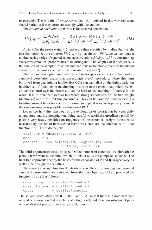
Let us see how this plays out in the exploration of covariation between dailytemperature and log precipitation, being careful to avoid the greediness pitfall byplacing very heavy penalties on roughness of the canonical weight functions asmeasured by the size of their second derivatives. Here are the commands in R thatfunction cca.fd to do the job:

ccafdPar = fdPar(daybasis, 2, 5e6)ncon = 3ccalist = cca.fd(temp.fd, logprec.fd, ncon,

ccafdPar, ccafdPar)

The third argument of cca.fd specifies the number of canonical weight/variablepairs that we want to examine, which, in this case, is the complete sequence. Thefinal two arguments specify the bases for the expansion of ξ and η , respectively, aswell as their roughness penalties.

The canonical weight functional data objects and the corresponding three squaredcanonical correlations are extracted from the list object ccalist produced byfunction cca.fd as follows:

ccawt.temp = ccalist$ccawtfd1ccawt.logprec = ccalist$ccawtfd2corrs = ccalist$ccacorr

The squared correlations are 0.92, 0.62 and 0.35; so that there is a dominant pairof modes of variation that correlates at a high level, and then two subsequent pairswith modest but perhaps interesting correlations.


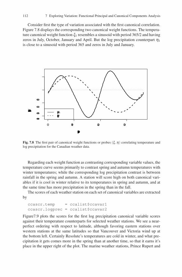
Consider first the type of variation associated with the first canonical correlation.Figure 7.8 displays the corresponding two canonical weight functions. The tempera-ture canonical weight function ξ1 resembles a sinusoid with period 365/2 and havingzeros in July, October, January and April. But the log precipitation counterpart η1is close to a sinusoid with period 365 and zeros in July and January.

0 100 200 300

−0.1

0−0

.05

0.00

0.05

Day (July 1 to June 30)

Can

onic

al W

eigh

t Fun

ctio

n

Temp.Log Prec.

Fig. 7.8 The first pair of canonical weight functions or probes (ξ ,η) correlating temperature andlog precipitation for the Canadian weather data.

Regarding each weight function as contrasting corresponding variable values, thetemperature curve seems primarily to contrast spring and autumn temperatures withwinter temperatures; while the corresponding log precipitation contrast is betweenrainfall in the spring and autumn. A station will score high on both canonical vari-ables if it is cool in winter relative to its temperatures in spring and autumn, and atthe same time has more precipitation in the spring than in the fall.

The scores of each weather station on each set of canonical variables are extractedby

ccascr.temp = ccalist$ccavar1ccascr.logprec = ccalist$ccavar2

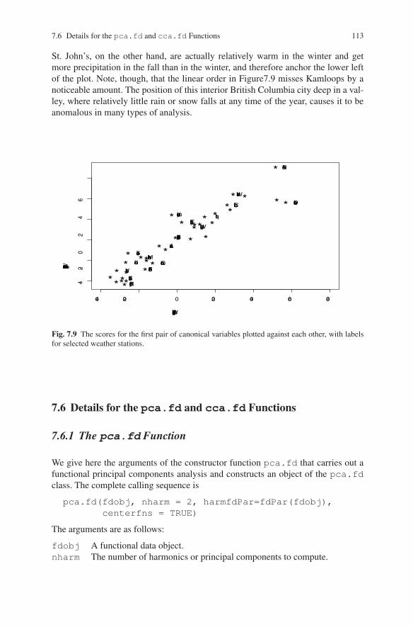
Figure7.9 plots the scores for the first log precipitation canonical variable scoresagainst their temperature counterparts for selected weather stations. We see a near-perfect ordering with respect to latitude, although favoring eastern stations overwestern stations at the same latitudes so that Vancouver and Victoria wind up atthe bottom left. Certainly Resolute’s temperatures are cold in winter, and what pre-cipitation it gets comes more in the spring than at another time, so that it earns it’splace in the upper right of the plot. The marine weather stations, Prince Rupert and

7.6 Details for the pca.fd and cca.fd Functions 113

St. John’s, on the other hand, are actually relatively warm in the winter and getmore precipitation in the fall than in the winter, and therefore anchor the lower leftof the plot. Note, though, that the linear order in Figure7.9 misses Kamloops by anoticeable amount. The position of this interior British Columbia city deep in a val-ley, where relatively little rain or snow falls at any time of the year, causes it to beanomalous in many types of analysis.

**** * *

** *

******

**

**

* **

***

**

*

*

**

*

*

*

*

−40 −20 0 20 40 60 80

−4−2

02

46

Temperature Canonical Weight

Log

Pre

cipi

tatio

n C

anon

ical

Wei

ght

Resolute

Whitehorse

DawsonChurchill

IqaluitKamloopsCalgary

Winnipeg

Thunder Bay

ArvidaToronto

MontrealLondon Quebec

Victoria Fredericton

St. JohnsPr. Rupert

Fig. 7.9 The scores for the first pair of canonical variables plotted against each other, with labelsfor selected weather stations.

7.6 Details for the pca.fd and cca.fd Functions

7.6.1 The pca.fd Function

We give here the arguments of the constructor function pca.fd that carries out afunctional principal components analysis and constructs an object of the pca.fdclass. The complete calling sequence is

pca.fd(fdobj, nharm = 2, harmfdPar=fdPar(fdobj),centerfns = TRUE)

The arguments are as follows:

fdobj A functional data object.nharm The number of harmonics or principal components to compute.


harmfdPar A functional parameter object that defines the harmonic or principalcomponent functions to be estimated.

centerfns A logical value: if TRUE, subtract the mean function from eachfunction before computing principal components.

Function pca.fd returns an argument of the pca.fd class, which is a namedlist with the following components:

harmonics A functional data object for the harmonics or eigenfunctions.values The complete set of eigenvalues.scores A matrix of scores on the principal components or harmonics.varprop A vector giving the proportion of variance explained by each eigen-

function.meanfd A functional data object giving the mean function.

7.6.2 The cca.fd Function

The calling sequence for cca.fd is

cca.fd(fdobj1, fdobj2=fdobj1, ncan = 2,ccafdParobj1=fdPar(basisobj1, 2, 1e-10),ccafdParobj2=ccafdParobj1, centerfns=TRUE)

The arguments are as follows:

fdobj1 A functional data object.fdobj2 A functional data object. By default this is fdobj1, in which case the

first argument must be a bivariate functional data object.ncan The number of canonical variables and weight functions to be computed.

The default is 2.ccafdParobj1 A functional parameter object defining the first set of canonical

weight functions. The object may contain specifications for a roughness penalty.The default is defined using the same basis as that used for fdobj1 with a slightpenalty on its second derivative.

ccafdParobj2 A functional parameter object defining the second set of canon-ical weight functions. The object may contain specifications for a roughnesspenalty. The default is ccafdParobj1.

centerfns If TRUE, the functions are centered prior to analysis. This is thedefault.

7.7 Some Things to Try

1. Medfly Data: The medfly data have been a popular dataset for functional dataanalysis and are included in the fda package. The medfly data consist of records

7.8 More to Read 115

of the number of eggs laid by 50 fruit flies on each of 31 days, along with eachindividual’s total lifespan.

a. Smooth the data for the number of eggs, choosing the smoothing parameterby generalized cross-validation (GCV). Plot the smooths.

b. Conduct a principal components analysis using these smooths. Are the com-ponents interpretable? How many do you need to retain to recover 90% of thevariation. If you believe that smoothing the PCA will help, do so.

c. Try a linear regression of lifespan on the principal component scores fromyour analysis. What is the R2 for this model? Does lm find that the model issignificant? Reconstruct and plot the coefficient function for this model alongwith confidence intervals. How does it compare to the model obtained throughfunctional linear regression?

2. Apply principal components analysis to the functional data object Wfd re-turned by the monotone smoothing function smooth.monotone applied tothe growth data. These functions are the logs of the first derivatives of the growthcurves. What is the impact of the variation in the age of the purbertal growthspurt on these components?

7.8 More to Read

Functional principal components analysis predates the emergence of functional dataanalysis, especially in fields in engineering and sciences that work with functionaldata routinely, such as climatology. Principal components are often referred to inthese fields as empirical basis functions, a phrase that is exactly the right thing sincefunctional principal components are both orthogonal and can also serve well as acustomized low-dimensional basis system for representing the actual functions.

There are many currently active and unexplored areas of research into functionalPCA. James et al. (2000) consider situations where curves are observed in frag-ments, so that the interval of observation varies from record to record. James andSugar (2003) look at the same data situation in the context of cluster analysis, an-other multivariate exploratory tool that is now associated with a large functional lit-erature. Readers with a background in psychometrics will wonder about a functionalversion of factor analysis, whether exploratory or confirmatory; and functional ver-sions of structural equation models are well down the road, but no doubt perfectlyfeasible.

chapter 7 exploring variation: functional principal and...

Documents