chapter 2 production planning and scheduling: interaction ... · pdf file2 production planning...

Chapter 2Production Planning and Scheduling:Interaction and Coordination

Yiwei Cai, Erhan Kutanoglu, and John Hasenbein

2.1 Introduction

In many organizations, production planning is part of a hierarchical planning,capacity/resource allocation, scheduling and control framework. The productionplan considers resource capacities, time periods, supply and demand over a rea-sonably long planning horizon at a high level. Its decision then forms the inputto the more detailed, shorter-term functions such as scheduling and control at thelower level, which usually have more accurate estimates of supply, demand, andcapacity levels. Hence, interaction between production planning and productionscheduling/control is inevitable, not only because the scheduling/control decisionsare constrained by the planning decisions, but also because disruptions occurringin the execution/control stage (usually after schedule generation) may affect theoptimality and/or feasibility of both the plan and the schedule. If the overall per-formance of the production system is to be improved, disruptions must be managedeffectively, with careful consideration of both planning and scheduling decisions.This chapter focuses on the interaction between production planning and schedul-ing, emphasizing the coordination of decisions, with special emphasis on makingrobust decisions at both levels in the face of unexpected disruptions. We provideexamples and realistic scenarios from semiconductor manufacturing.

To capture the interaction between production planning and scheduling, wesuggest an intermediate model between the two levels. One can view this as a lower-level planning model or a higher-level scheduling model, but ultimately it providesa middle ground between the two levels of the decision-making framework. In manysystems, the longer-term, aggregated production plan is used to facilitate scheduling.This is usually achieved by creating specific work orders or jobs of different producttypes that collectively resemble the output required by the production plan and gen-erating a release schedule for the jobs. For example, semiconductor manufacturers

E. Kutanoglu (�)Graduate Program in Operations Research and Industrial Engineering,Department of Mechanical Engineering, The University of Texas at Austin, Austin,TX 78712, USAe-mail: [email protected]

K.G. Kempf et al. (eds.), Planning Production and Inventories in the ExtendedEnterprise, International Series in Operations Research & Management Science 152,DOI 10.1007/978-1-4419-8191-2 2, c� Springer Science+Business Media, LLC 2011

15

[email protected]

16 Y. Cai et al.

rely on detailed simulation-based models to fine tune the release schedule (alsoreferred to as “wafer starts”), which ultimately determines the product mix in thewafer fab. The scheduling function typically dispatches the jobs according to theirperceived or assigned priorities to align the processing sequence of the jobs with theproduction plan while using the latest information on job and machine availabilities.Dispatching inherently utilizes local information (typically one-job, one-machine ata time) to make a decision. It is very hard, if not impossible, to calculate the effectsof an individual dispatching decision on the long-term system performance, or evenon the performance of the upstream and downstream machines on the shop floor.The idea of an intermediate model between planning and scheduling is to provideadditional useful information to the scheduling system, whether it is dispatchingbased or otherwise.

With the interaction and coordination between production planning and schedul-ing being the main theme of this chapter, we first review the literature, focusing ona selected set of production planning and scheduling-based papers. In Sect. 2.3, wepresent two versions of our approach that attempt to fill the gap between the classicalplanning and dispatching-based scheduling models using an intermediate decisionmodel. Section 2.4 describes our computational study with a simplified reentrantsystem that represents a small wafer fabrication facility. Section 2.4 also discussesthe implementation issues that must be addressed to properly compare the proposedapproach with the conventional planning-to-scheduling approach, using this mini-fab model. In Sect. 2.5, we present the experimental results focusing on insights thatcan be obtained from our preliminary experiments. We conclude with a summaryand future research directions in Sect. 2.6.

2.2 Literature Review

We first review the production planning models that are representative of the existingmodels in the literature. This review is not exhaustive by any means, and our mainfocus is on the interaction between planning and scheduling, not necessarily on theother aspects of the models, such as batching or setups, that may be potentiallycritical. We also try to give examples and applications from the literature on semi-conductor manufacturing to make the discussion more concrete, but the methodsdiscussed in this section also pertain to more discrete parts manufacturing systems.Due to increasing competition and the rapid development of technology, manufac-turing managers, especially those in semiconductor industry focus strongly on cycletime, which is defined as the time between the release of an order to the shop floorand its completion time of that order. Long cycle times imply a high work-in-process(WIP) level, and thus high inventory costs. Therefore, we choose cycle time as themain performance measure with which we evaluate the effectiveness of the coor-dination between planning and scheduling. This choice further limits our literaturereview to studies that emphasize cycle time as a potential issue to be addressedbetween planning and scheduling.

2 Production Planning and Scheduling: Interaction and Coordination 17

2.2.1 Production Planning Models

An extensive literature on production planning has been developed over almost fivedecades. In this section, we focus on only a few of these optimization models.Interested readers are referred to the chapter by Missbauer and Uzsoy (2010) in thefirst volume of this handbook which reviews the basic formulations that are mostcommonly used in academic research and industrial practice.

A capacitated Material Requirement Planning (MRP)-based model is proposedby Horiguchi et al. (2001). The goal is to calculate a planned release date for eachorder during each of its visits to a bottleneck station, and to estimate when the orderwill be completed. The authors aggregate the times available across machines overdiscrete time periods (time buckets) that are used to incorporate capacity factors.The model explicitly considers capacity only for specified near-bottleneck stations,and assumes that all other stations have infinite capacity, which is different fromthe conventional MRP approach. They perform two experiments. One examines theeffect of the predictability of the capacity model. In their paper, predictability is de-fined as the deviation of the realized completion time in the simulation model fromthe predicted completion time in the planning model. The results show that finitecapacity planning gives better predictability than dispatching rules such as CriticalRatio (Rose 2002). The lot with the lowest value has the highest priority. The sec-ond experiment tests the effects of using a “safety capacity” in planning, that is, thereduction of the planned capacity of a given station by some amount to keep process-ing capacity in reserve to deal with unexpected events such as machine breakdowns.Their results show that increasing the safety capacity reduces tardiness and improvespredictability, without adversely affecting other performance measures.

There are a wide variety of linear programming-based planning models forproduction planning. Hackman and Leachman (1989) propose a general productionplanning framework based on a linear programming model. They take into consid-eration specific components such as processing and transfer time in order to providean accurate representation of the production process. However, the time delays in themodel do not capture the load-dependent nature of the lead times. Thus, the aspectsof production captured in the model are limited. In addition, the LP formulationaccommodates noninteger values for cycle times as well as planning time bucketsof unequal length. Expanding the model in Hackman and Leachman (1989), Hungand Leachman (1996) incorporate time-dependent parameters representing partialcycle times from job release up to each operation into the LP planning model. Fur-thermore, they provide a framework that iteratively updates the plan through an LPmodel that develops a plan for a given set of lead times and a simulation modelthat evaluates the system performance for a given production plan. They estimatethe cycle times from the simulation results and show that they can achieve betterresults by iterating between the LP and the simulation model. It is well known thatthe relationship between cycle time and machine utilization is nonlinear. Therefore,the iterative LP-simulation process provides a good way to approximate such a non-linear relationship. The process stops when satisfactory agreement in cycle timesis achieved. Hung and Leachman’s experiments with deterministic and random

18 Y. Cai et al.

machine breakdowns indicate that the difference between the LP and simulationcycle times can be reduced to 5% or less within a few iterations. However, otherresearchers have not been able to easily replicate such results, and our own researchindicates that similar results are difficult to achieve. In particular, the convergencebehavior appears to be unpredictable, and is certainly not well understood.

Some planning models that try to capture the relationship between cycle time andutilization without resorting to simulation make use of so-called clearing functions(Graves 1986). Clearing functions express the expected throughput of a machine ina planning period as a function of the expected WIP inventory at the machine overthe period. (Our focus on load-dependent cycle times is mainly due to the obser-vation that the load as a function of releases determined as part of the plan affectscycle times that result in scheduling. There are recent studies that try to capturethe dependency between the load level and/or utilization and cycle times. In thatsense, the underlying approaches can also be viewed as “hybrid” models attempt-ing to link planning and scheduling.) Missbauer (2002) considers clearing functionsfor an M/G/1 system. He uses a piece-wise linear approximation for the clearingfunction to model the effective capacity for bottleneck stations, and considers fixed,load-independent time delays between bottleneck stages to represent the delays atnonbottleneck machines. His planning model determines the release plan and uses ashort-term order release policy to select specific orders for release into the job shop.The product mix is not considered in their clearing function, i.e., the clearing func-tion only depends on the total planned production quantity, which means the totaloutput of a station can be allocated arbitrarily to different products.

Asmundsson et al. (2006) propose a clearing function-based planning model,which explicitly considers the product mix. They approximate the clearing func-tion using an empirical approach, together with two sets of constraints enforcingflow conservation for WIP and finished goods inventory (FGI). There is no needfor explicit cycle time parameters in their model. Due to the product mix, differentproducts may have different capacity needs (capacity allocation), and a particulardifficulty is estimating the throughput as a function of the product mix currentlyrepresented in the WIP. To overcome this, they assume that all products see the sameaverage cycle time, which allows them to use a convex combination of the capacityallocation parameters to approximate the WIP levels of different products, which inturn leads to approximated clearing functions. Exploiting the concavity of clearingfunctions, they use outer linearization to approximate the functions, which results inan LP model. The objective in their model is to minimize the total production cost,the WIP cost, the FGI holding cost, and the raw material cost. The approximationof the clearing function is also done by simulation with several randomly generatedrealizations of the demand profile, which are evaluated using the release schedulesobtained from the fixed cycle time production planning model of Hackman andLeachman (1989). They perform extensive experiments to evaluate the benefit ofthe clearing function-based model. Different dispatching rules are used to compareplanned throughput and actual throughput. Based on these experiments, one of theirconclusions is that:


“If planning is done properly, the role of a detailed schedule can be viewed as reschedulingthe jobs to adhere to the original production plan that has been distorted by equipmentfailures and other unpredictable occurrences. Although it is unlikely that the scheduler canrestore the original plan in every instance, its ability to do so is highly dependent on theplanning algorithm’s ability to represent the shop floor dynamics correctly.”

Such a conclusion shows that we need to consider the coordination betweenplanning and scheduling to achieve better performance, which further motivatesour study.

Pahl et al. (2005) give an extensive survey of planning models, which considerload-dependent cycle times. In addition to the use of clearing functions, there areother approaches. Interested readers are referred to Sect. 3 and the correspondingreferences in Pahl et al. (2005) for more details.

Model predictive control, or MPC (Qin and Badgwell 2003), is a method ofprocess control that has been used extensively in processing industries (Kleindorferet al. 1975). MPC encompasses a group of algorithms that optimize the predicted fu-ture values of the plant output by computing a sequence of future control increments.This optimization model is implemented through a rolling-horizon approach at eachsampling time. MPC attempts to model the dependence between the sequence ofpredicted values of the system output, and the sequence of future control increments.With knowledge of the system model, disturbance measurements, and historicalinformation of the process, the MPC model calculates a sequence of future con-trol increments that must satisfy appropriate constraints. Vargas-Villami and Rivera(2000) propose a two-layer production control method based on MPC. Extendingthis work, Vargas-Villami et al. (2003) propose a three-layer version. The first layer,called the adaptive layer, is used to develop a parameter estimation approach. Thesecond layer, the optimizer, solves an MILP model by branch and bound to gener-ate a good-quality production plan. The third layer (direct control) uses dispatchingto control the detailed discrete-event reentrant manufacturing line in a simulationmodel. The computational results show that the method is less sensitive to initialconditions than “industrial-like” policies examined by Tsakalis et al. (2003). Fur-thermore, the three-layer approach with the adaptive parameter estimation modelachieves reduced variation at high production loads as compared to the two-layerapproach. They did not perform any cycle time comparisons with existing methods,but point out that an MPC-based model could be a promising tool for planning.

Jaikumar (1974) proposes a methodology, which decomposes the planning andscheduling problem into two subproblems. The first problem is a long range plan-ning problem, which maximizes the profit subject to resource constraints. The La-grange multiplers obtained in the first problem are used in the objective function ofthe second short range scheduling model. They propose a heuristic algorithm to re-duce the second model to a sequential allocation of production facilities to products.

2.2.2 Scheduling Models

Apart from planning models, there are models and studies that focus on schedulingonly. Leachman et al. (2002) summarize their effort, dubbed Short Cycle Time

20 Y. Cai et al.

and Low Inventory in Manufacturing (SLIM), to improve scheduling at SamsungElectronics. They try to control the production line by managing the WIP level atparticular bottleneck stations. A dispatching-based method is used to achieve targetWIP levels at the bottleneck stations. An important task is to determine appropriatetarget WIP levels. Based on an overall target cycle time for each product, the totalbuffer time is calculated as the difference between the target cycle time and theoreti-cal (or raw) cycle time. The total buffer time is then proportionally allocated to eachbottleneck step. The resulting buffer time allocation is in turn used to estimate thetarget WIP levels using Little’s Law. By using different strategies according to thecharacteristics of different production stages (bottleneck, batching, nonbottlenecksteps, etc.) and prioritizing the jobs in different stages to meet target WIP levels(and hence bottleneck utilization) as closely as possible, they show that one canreduce average cycle times.

In contrast to the fab-wide approach in Leachman et al. (2002), other authorsfocus on bottleneck steps only, with explicit controls the WIP level. Lee and Kim(2002) try to implement WIP control at bottleneck steps to balance a productionline in semiconductor manufacturing. Assuming a given target throughput rate, theycalculate the buffer time and the associated target WIP level. The work focuses onshort-term scheduling for the steppers, which are usually the bottleneck machines inmost wafer fabrication facilities. One of the two proposed MILP models minimizesthe total weighted deviation from the target WIP level, and the other maximizesthe total wafer production for all steppers in the hope that this will lead to highutilization of bottleneck machines.

Kim et al. (2003) use a similar idea to determine a single-shift schedule for thesteppers for a given WIP status. Using an MILP formulation, they try to maintainthe WIP levels close to the “desired” levels so that the flow of material through thefactory is balanced. The objective is to meet the predetermined WIP targets. Threeproposed heuristics to solve the underlying MILP model can find schedules within5% of the optimum values in a reasonable amount of time.

Queueing theory is useful in scheduling in several ways. One way is to analyzethe stability (that is, boundedness of average WIP) of scheduling policies. An-other way is to model manufacturing systems with multiclass queueing networksto develop scheduling policies. Generally speaking, queueing theory is based onlong-term steady-state analysis and may not be optimal in a finite period. However,the following two papers implement queueing theory using fluid models that fo-cus on transient analysis and are a reasonable approximation for short periods oftime. Dai and Weiss (2002) develop a fluid-relaxation-based heuristic to minimizemakespan in job shops. In a fluid model, discrete jobs are replaced with flow of acontinuous fluid and machines are replaced with valves that affect the flow rate ofthe of fluid. The proposed online (dispatching-based) heuristic uses safety stocks forWIP and tries to keep the bottleneck machine busy at almost all times, with the ideathat the nonbottleneck machines are paced accordingly. The heuristic is constructedin three steps: (1) reduce the job shop problem to a reentrant line scheduling prob-lem, which has the same lower bound; (2) define an infeasible backlog schedulethat keeps the bottleneck machine busy (here the schedule is infeasible because a


machine is allowed to start work on a job step even if the previous step of the jobon a different machine has not been completed); (3) introduce safety stocks to makethe backlog schedule feasible.

Similarly, Bertsimas et al. (2003) use a fluid model to solve a job shop schedulingproblem with the objective of minimizing the holding cost. The proposed algorithmuses the optimal fluid solution as a guide. Comparison with several other commonlyused heuristics shows that the proposed algorithm outperforms the other heuristicmethods.

This section provided a brief review of planning and scheduling models with afocus on the interaction between the two models. We note that most of the plan-ning models in the literature do not consider WIP allocation across stations, whilemany scheduling models consider WIP level explicitly. Therefore, we propose anapproach in Sect. 2.3 to explicitly consider WIP allocation in an intermediate modelcalled high-level scheduling, and try to control WIP allocation in a way which fa-cilitates the coordination between planning and scheduling.

2.3 Coordination of Planning and Scheduling

2.3.1 Overall Approach

In most manufacturing companies, the planning and scheduling functions belong totwo different departments, as planning is viewed as a tactical activity and schedulingas more operational. Sometimes it is necessary to separate planning and schedulingbecause it is almost impossible to obtain a comprehensive system-wide solution thatencompasses both planning and scheduling concerns. Such a model would have toprovide detailed decisions for each machine in each period. In general, it is im-possible to solve such a model since it is inherently too complex with too manyconstraints and variables. Hierarchical decomposition into planning and schedulingprovides an easy way not only to obtain reasonable solutions to both subproblems,but also to generate decisions aligned with the current organizational structure be-tween planning and scheduling functions.

However, the conventional hierarchical separation of these two functions maycause several problems. One drawback is that a solution that is good at the planninglevel might not be easy to implement as a detailed schedule; the plan may not beeven feasible when the scheduling issues are explicitly considered. One reason be-hind this is that the dynamics of the production system are modeled at an aggregatelevel, and detailed execution may be infeasible even if aggregate constraints are sat-isfied. Another issue is that objectives are usually different between planning andscheduling. The planning function focuses more on how to meet the demand, andreduce inventory and backorders, while scheduling emphasizes more operationalmeasures such as minimizing cycle times and maximizing bottleneck utilization.Ideally, if the hierarchical decomposition were done properly, the objectives of thetwo levels would be aligned. However, due to the complexity of the overall problem,

22 Y. Cai et al.

the computational effort involved in solving the two levels to optimality, and thedifferences in preferences between the organizational areas representing the twolevels, this is not the case in the real world.

In this chapter, we test an idea that seeks to overcome the drawbacks of suchseparation of planning and scheduling. The idea is to introduce an “intermediate”module between planning and scheduling, which overall modifies the conventionalhierarchical approach. The goal is to solve the discrepancy in objectives betweenproduction planning and detailed scheduling. In the following, we define “normalplanning” as a planning model that does not consider WIP levels explicitly, and a“high level scheduling” model as one that does. In this approach, we have a normalplanning model (denoted by “P”) and a high level scheduling model (denoted by“H”) that both feed into detailed scheduling (denoted by “D”) (See Fig. 2.1). Toprovide a framework for our discussion, we represent each “stage” in the processwith an associated model: the planning model, the high-level scheduling model,and the detailed scheduling model. In fact, in the following discussion, the first twomodels are linear programming problems and the last one is a simulation model ofthe system that represents the actual implementation of the plan and schedule.

First, we explain the proposed version of the P–H–D approach: The planningmodel tries to meet the demand while minimizing inventory and backorder costs.The output of the planning model specifies how much of each product should beproduced by the end of each period. Then, we use that output as a modified demandprofile, which is input to the high level scheduling model, which explicitly triesto minimize the average WIP level, and thus the average cycle time. The high levelscheduling model determines the release policy and processing targets for each prod-uct in each period, which form the input to detailed scheduling. Figure 2.1 comparesthe proposed P–H–D approach with the P–D approach.

Fig. 2.1 Three approaches for planning and scheduling


Consideration of the three potential levels in the overall process gives rise toanother structure, in which the planning step is skipped: the original demand datais fed directly to the high-level scheduling model whose output is input to the de-tailed scheduling model. Intuitively, using a high level schedule without a planningmodel consideration may achieve lower cycle times, but may result in higher costssince it pays more direct attention to WIP levels than to costs. We now discuss ourmathematical formulations for the planning and high level scheduling models.

2.3.2 Planning Model

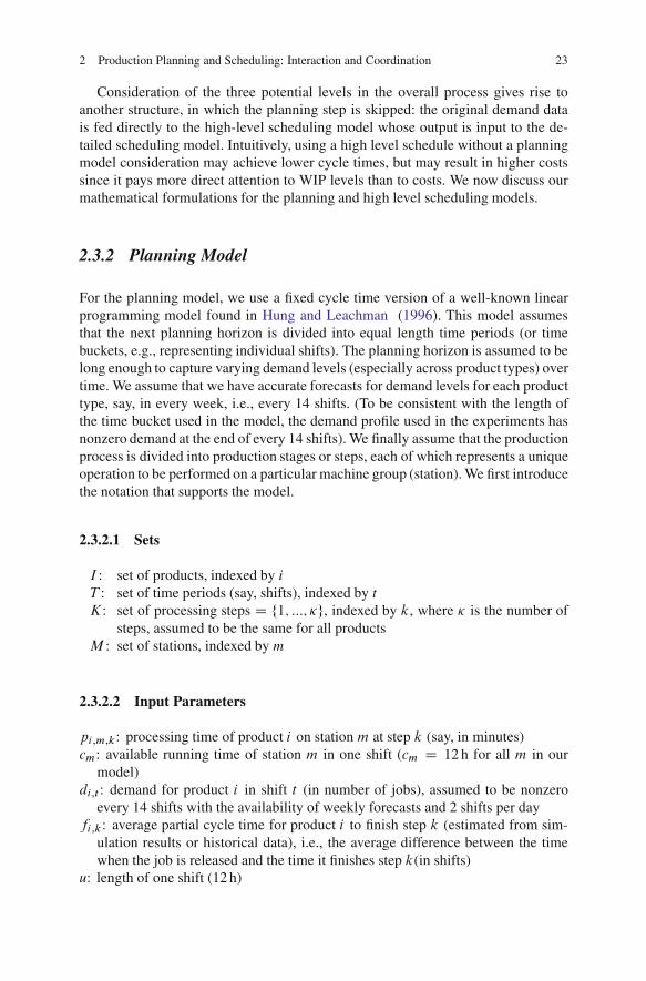
For the planning model, we use a fixed cycle time version of a well-known linearprogramming model found in Hung and Leachman (1996). This model assumesthat the next planning horizon is divided into equal length time periods (or timebuckets, e.g., representing individual shifts). The planning horizon is assumed to belong enough to capture varying demand levels (especially across product types) overtime. We assume that we have accurate forecasts for demand levels for each producttype, say, in every week, i.e., every 14 shifts. (To be consistent with the length ofthe time bucket used in the model, the demand profile used in the experiments hasnonzero demand at the end of every 14 shifts). We finally assume that the productionprocess is divided into production stages or steps, each of which represents a uniqueoperation to be performed on a particular machine group (station). We first introducethe notation that supports the model.

2.3.2.1 Sets

I : set of products, indexed by iT : set of time periods (say, shifts), indexed by tK: set of processing steps D f1; :::; �g, indexed by k, where � is the number of

steps, assumed to be the same for all productsM : set of stations, indexed by m

2.3.2.2 Input Parameters

pi;m;k: processing time of product i on station m at step k (say, in minutes)cm: available running time of station m in one shift (cm D 12 h for all m in our

model)di;t : demand for product i in shift t (in number of jobs), assumed to be nonzero

every 14 shifts with the availability of weekly forecasts and 2 shifts per dayfi;k: average partial cycle time for product i to finish step k (estimated from sim-

ulation results or historical data), i.e., the average difference between the timewhen the job is released and the time it finishes step k(in shifts)

u: length of one shift (12 h)

24 Y. Cai et al.

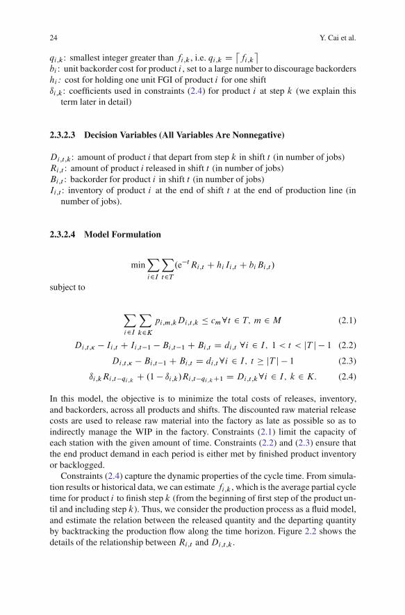
qi;k: smallest integer greater than fi;k , i.e. qi;k D ˙fi;k

�

bi : unit backorder cost for product i , set to a large number to discourage backordershi : cost for holding one unit FGI of product i for one shiftıi;k: coefficients used in constraints (2.4) for product i at step k (we explain this

term later in detail)

2.3.2.3 Decision Variables (All Variables Are Nonnegative)

Di;t;k: amount of product i that depart from step k in shift t (in number of jobs)Ri;t : amount of product i released in shift t (in number of jobs)Bi;t : backorder for product i in shift t (in number of jobs)Ii;t : inventory of product i at the end of shift t at the end of production line (in

number of jobs).

2.3.2.4 Model Formulation

minX

i2I

X

t2T

.e�tRi;t C hi Ii;t C biBi;t /

subject to

X

i2I

X

k2K

pi;m;kDi;t;k � cm8t 2 T; m 2 M (2.1)

Di;t;� � Ii;t C Ii;t�1 � Bi;t�1 C Bi;t D di;t 8i 2 I; 1 < t < jT j � 1 (2.2)

Di;t;� � Bi;t�1 C Bi;t D di;t8i 2 I; t � jT j � 1 (2.3)

ıi;kRi;t�qi;kC .1 � ıi;k/Ri;t�qi;kC1 D Di;t;k8i 2 I; k 2 K: (2.4)

In this model, the objective is to minimize the total costs of releases, inventory,and backorders, across all products and shifts. The discounted raw material releasecosts are used to release raw material into the factory as late as possible so as toindirectly manage the WIP in the factory. Constraints (2.1) limit the capacity ofeach station with the given amount of time. Constraints (2.2) and (2.3) ensure thatthe end product demand in each period is either met by finished product inventoryor backlogged.

Constraints (2.4) capture the dynamic properties of the cycle time. From simula-tion results or historical data, we can estimate fi;k , which is the average partial cycletime for product i to finish step k (from the beginning of first step of the product un-til and including step k). Thus, we consider the production process as a fluid model,and estimate the relation between the released quantity and the departing quantityby backtracking the production flow along the time horizon. Figure 2.2 shows thedetails of the relationship between Ri;t and Di;t;k.


Fig. 2.2 Partial cycle times, and the relationship between Ri;t and Di;t;k

All products of type i finished at step k in shift t , denoted by Di;t;k shouldhave been released fi;k time units ago. Thus, by backtracking we can determine thetime when these products are released. In Hung and Leachman (1996), a formula isprovided to address all the cases where the cycle time is either longer or shorter thanthe length of the time bucket. Since we use a constant length for each time bucket,and in our mini-fab model (see Sect. 2.4.1) the partial cycle times are less than thelength of the time bucket (shift), Di;t;k is composed of two parts. Thus, the relationbetween the products released, Ri;t , and Di;t;k is as follows:

Di;t;k D ıi;kRi; t�qi;kC .1 � ıi;k/Ri; t�qi;kC1 8i 2 I; 1 � t � jT j � 1; k 2 K;

where the portions of releases to be completed by step k are estimated by ıi;k and(1 � ıi;k). Here, we use ıi;k’s proportional to time: ıi;k D .fi;k mod u/=u, 8i 2 I

and 8k 2 K .

2.3.3 High Level Scheduling Model

As mentioned before, the purpose of the high level scheduling model is to find a bal-ance between the cycle times and the inventory/backorder costs. Thus, its objectivefunction and constraints should take both factors into consideration. Although it ishard to model cycle times directly, we know from Little’s Law that they are propor-tional to WIP levels for a fixed throughput. Thus, we consider the WIP level insteadand try to represent minimization of cycle times by minimizing the WIP levels atthe end of each shift.

26 Y. Cai et al.

In this model, the relationship between releases and departures is captured in thesame manner as in the planning model. The main difference is that we explicitlycapture WIP levels and their distribution across stations and stages of production indetail. In this model, we manage to keep a certain level of WIP at bottleneck stationto prevent its starvation, which may lead to reductions in the throughput rate. Theselevels are formulated using a WIP control constraint that allows the WIP to be withina tolerance around the target value. To enable the model to build up WIP to meet thetarget level, the LP model enforces the WIP control constraints only after a certainnumber of periods elapsed. With this in mind, we introduce additional notation.

2.3.3.1 Sets

KB : set of steps in the bottleneck station

2.3.3.2 Input Parameters

�C; ��: upper and lower tolerance of WIP control (currently set at �C D 1:1 and�� D 0:9)

vi : target cycle time for product i (in minutes)�i : total raw processing time for product i (in minutes)yi : total buffer time for product i , i.e. the difference between the vi and �i (in

minutes)zi;k: target WIP level of product i at station k (in number of jobs)�i;k: the average cycle time for product i to travel to the kth bottleneck step from

its previous bottleneck step (in minutes)�i : average demand rate for product i (in jobs per minute)ts : the last shift in which the WIP control constaints are not enforced; the high level

scheduling model is assumed to be in steady state after shift ts

2.3.3.3 Decision Variables

Wi;t;k: WIP level of product i at step k at the end of shift t (in number of jobs).

2.3.3.4 Model Formulation

The calculation of the target WIP level is adapted from the method proposed byLeachman et al. (2002), which uses Little’s Law (as will be explained in detaillater). They use target WIP levels as criteria for dispatching. Here, we incorpo-rate the target WIP levels into the high level scheduling model. The target WIPcalculation allocates the buffer time to bottleneck steps in proportion to the par-tial cycle time between two consecutive bottleneck steps. Cycle times are estimated


from a simulation model of the mini-fab in our experiments, but practice they can beobtained from historical data. One can calibrate the estimated cycle times throughmultiple simulation runs, but here we obtain cycle times in a single run. We firstcompute the buffer time as the difference between the target cycle time and thetheoretical (or raw) cycle time (which consists of only processing times) for eachproduct:

yi D vi � �i 8i 2 I:

To allocate this overall buffer time (slack) into bottleneck steps, we compute thetime between two consecutive bottleneck steps of each product:

�i;k D fi;k � fi;k0 8i 2 I; k; k0 2 KB;

where k and k0 are two consecutive bottleneck steps.Finally, we set the target throughputs equal to the average demand rates, allocate

the overall buffer time and convert the allocations to target WIP levels as follows:

zi;k D �i � yi � �i;kX

k02KB

�i;k0

8i 2 I; k 2 KB :

The final mathematical model is as follows:

minX

i2I

X

t2T

X

k2K

Wi;t;k C hi Ii;t C bi Bi;t

!

subject toX

t2T

X

k2K

pi;m;kDi;t;k � cm; 8t 2 T; m 2 M (2.5)

Di;t;� � Ii;t C Ii;t�1 � Bi;t�1 C Bi;t D di;t ; 8i 2 I; 1 < t < jT j � 1 (2.6)

Di;t;� � Bi;t�1 C Bi;t D di;t ; 8i 2 I; t � jT j � 1 (2.7)

Ri;t � Di;t;1 C Ii;t;1 D Wi;t;1; 8i 2 I; t � 1 (2.8)

Di;t;k�1 � Di;t;k C Ii;t;k D Wi;t;k; 8i 2 I; t > 1; k > 1 (2.9)X

i2I

Wi;t;k � �C �X

i2I

zi;k; 8t 2 T; k 2 KB (2.10)

X

i2I

Wi;t;k � �� X

i2I

zi;k; 8t 2 t; k 2 KB (2.11)

ıi;kRi; t�qi;kC .1 � ıi;k/Ri; t�qi;kC1 � Di;j;k; 8i 2 I; 1 � t � ts k 2 K

(2.12)

ıi;kRi; t�qi;kC .1 � ıi;k/Ri; t�qi;kC1 D Di;j;k; 8i 2 I; ts < t � jT j � 1 k 2 K:

(2.13)

28 Y. Cai et al.

The main difference between this model and the previous planning-based one isthat we now have WIP control constraints for the bottleneck steps. Here, we firstcalculate the target WIP level for each step in the bottleneck station, and then usethe target WIP level in the LP model. Leachman et al. (2002) use a dispatching ruleto execute WIP control for individual buffers (product and step), while in our LPmodel we control the total WIP level across all products at the same step in thebottleneck station. The reason is that we think the purpose of setting target WIPlevels is to keep feeding the bottleneck station, so we only need to track the totalWIP level across all products at the same step in the bottleneck station instead ofcontrolling WIP levels for individual buffers.

2.4 Experimental Study

To test the idea of high level scheduling, we perform several experiments on a three-station six-step hypothetical production system, which represents a small waferfabrication facility (mini-fab). Below, we first describe the mini-fab system, and thenpresent the experimental results. These experiments focus on (1) evaluating the over-all merit of the P–H–D approach, (2) testing the impact of different cost settings, and(3) testing the impact of machine breakdowns at nonbottleneck stations on the cycletimes and cost. For testing, we run the mathematical models that represent the plan-ning and/or high-level scheduling problems with the same inputs, and then evaluatethe system performance (cycle time, WIP levels, costs) with a simulation modelthat imitates the implementation of decisions made by the mathematical models.For this, the simulation model relies on a dispatching-based methodology that triesto follow the release and production targets set by the outputs of the mathemati-cal models. Thus, the dispatching logic in the simulation model acts as a detailedscheduling system.

2.4.1 Mini-Fab Model

The three-station six-step mini-fab model is depicted in Fig. 2.3. There are two dif-ferent products, each of which must complete six operational steps. Each step isto be performed by a machine at one of the stations. The process flows (routings),which are the same for both products, are also shown in Fig. 2.3.

Table 2.1 shows the basic settings of the raw processing times for each product ateach step (in minutes). The last column shows the total raw processing time (RPT)for both products. We consider a time horizon of 150 days, each day with 2 shiftsof 12 h, leading to a 300-shift long horizon. All the processing times are assumed tobe deterministic.

In the experiments with machine breakdowns, the first station’s machines mayfail. Times between failures follow an exponential distribution with a mean of 42 h.The repair times follow an exponential distribution with a mean of 45 min. The base


Fig. 2.3 Six-step three-station mini-fab model

Table 2.1 Raw processing time for the mini-fab model

Step 1 Step 2 Step 3 Step 4 Step 5 Step 6 Total RPT

Product 1 47.5 30 75 40 52.5 30 275Product 2 38 24 60 32 42 24 220

Table 2.2 Traffic intensity(expected utilization)for all stations

Traffic intensity Station 1 Station 2 Station 3

No machine breakdowns 0.78 0.74 0.94With machine breakdowns 0.80 0.74 0.94

demand rates are 55 jobs per week for product 1 and 44 jobs per week for product 2.The backorder cost is $50 per unit per shift, and the inventory cost is $1 per unitper shift. We vary these values in the next section to evaluate impacts from differentfactors.

Table 2.2 gives the traffic intensities (or utilizations) with and without machinebreakdowns for all stations. We observe that station 3 is an overall bottleneck, andeven when breakdowns are considered, the bottleneck station does not change.

2.4.2 Simulation Settings

To evaluate the performances of the different approaches in combining planningand scheduling, we use a simulation model that imitates the execution of theplanning/scheduling decisions using a dispatching-based methodology. Here, thesimulation model represents the actual system, where the planning/scheduling deci-sions are executed at the detailed scheduling level, during which the actual costs andperformances are incurred and measured. The simulation model first creates pro-duction jobs according to the release schedule obtained in the mathematical modelbeing used. It then dispatches the jobs at the machines with some level of adher-ence to the planning and scheduling decisions. Although there are several ways tocarry out dispatching for a given plan/schedule, we apply two different dispatchingrules: First-in-first-out (FIFO) and “target following.” FIFO dispatches the job thatarrives at the station earliest, when a machine at the station becomes free, and isused primarily as a benchmark. The target following rule tries to follow the plan-ning or high level scheduling production targets (captured by the optimal values of

30 Y. Cai et al.

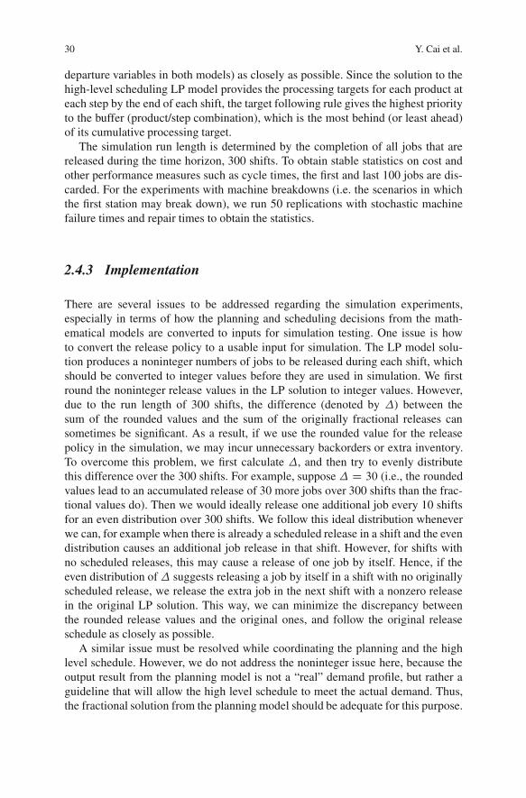
departure variables in both models) as closely as possible. Since the solution to thehigh-level scheduling LP model provides the processing targets for each product ateach step by the end of each shift, the target following rule gives the highest priorityto the buffer (product/step combination), which is the most behind (or least ahead)of its cumulative processing target.

The simulation run length is determined by the completion of all jobs that arereleased during the time horizon, 300 shifts. To obtain stable statistics on cost andother performance measures such as cycle times, the first and last 100 jobs are dis-carded. For the experiments with machine breakdowns (i.e. the scenarios in whichthe first station may break down), we run 50 replications with stochastic machinefailure times and repair times to obtain the statistics.

2.4.3 Implementation

There are several issues to be addressed regarding the simulation experiments,especially in terms of how the planning and scheduling decisions from the math-ematical models are converted to inputs for simulation testing. One issue is howto convert the release policy to a usable input for simulation. The LP model solu-tion produces a noninteger numbers of jobs to be released during each shift, whichshould be converted to integer values before they are used in simulation. We firstround the noninteger release values in the LP solution to integer values. However,due to the run length of 300 shifts, the difference (denoted by �) between thesum of the rounded values and the sum of the originally fractional releases cansometimes be significant. As a result, if we use the rounded value for the releasepolicy in the simulation, we may incur unnecessary backorders or extra inventory.To overcome this problem, we first calculate �, and then try to evenly distributethis difference over the 300 shifts. For example, suppose � D 30 (i.e., the roundedvalues lead to an accumulated release of 30 more jobs over 300 shifts than the frac-tional values do). Then we would ideally release one additional job every 10 shiftsfor an even distribution over 300 shifts. We follow this ideal distribution wheneverwe can, for example when there is already a scheduled release in a shift and the evendistribution causes an additional job release in that shift. However, for shifts withno scheduled releases, this may cause a release of one job by itself. Hence, if theeven distribution of � suggests releasing a job by itself in a shift with no originallyscheduled release, we release the extra job in the next shift with a nonzero releasein the original LP solution. This way, we can minimize the discrepancy betweenthe rounded release values and the original ones, and follow the original releaseschedule as closely as possible.

A similar issue must be resolved while coordinating the planning and the highlevel schedule. However, we do not address the noninteger issue here, because theoutput result from the planning model is not a “real” demand profile, but rather aguideline that will allow the high level schedule to meet the actual demand. Thus,the fractional solution from the planning model should be adequate for this purpose.


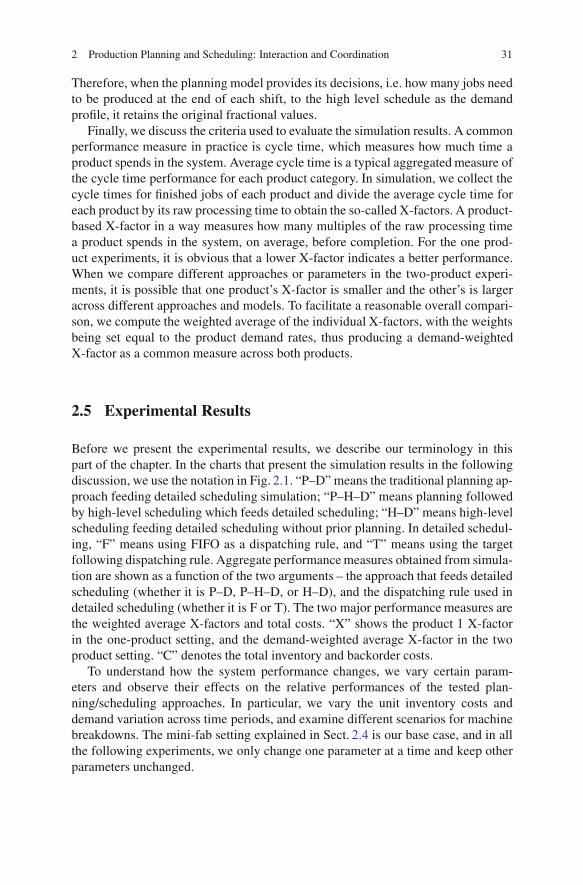
Therefore, when the planning model provides its decisions, i.e. how many jobs needto be produced at the end of each shift, to the high level schedule as the demandprofile, it retains the original fractional values.

Finally, we discuss the criteria used to evaluate the simulation results. A commonperformance measure in practice is cycle time, which measures how much time aproduct spends in the system. Average cycle time is a typical aggregated measure ofthe cycle time performance for each product category. In simulation, we collect thecycle times for finished jobs of each product and divide the average cycle time foreach product by its raw processing time to obtain the so-called X-factors. A product-based X-factor in a way measures how many multiples of the raw processing timea product spends in the system, on average, before completion. For the one prod-uct experiments, it is obvious that a lower X-factor indicates a better performance.When we compare different approaches or parameters in the two-product experi-ments, it is possible that one product’s X-factor is smaller and the other’s is largeracross different approaches and models. To facilitate a reasonable overall compari-son, we compute the weighted average of the individual X-factors, with the weightsbeing set equal to the product demand rates, thus producing a demand-weightedX-factor as a common measure across both products.

2.5 Experimental Results

Before we present the experimental results, we describe our terminology in thispart of the chapter. In the charts that present the simulation results in the followingdiscussion, we use the notation in Fig. 2.1. “P–D” means the traditional planning ap-proach feeding detailed scheduling simulation; “P–H–D” means planning followedby high-level scheduling which feeds detailed scheduling; “H–D” means high-levelscheduling feeding detailed scheduling without prior planning. In detailed schedul-ing, “F” means using FIFO as a dispatching rule, and “T” means using the targetfollowing dispatching rule. Aggregate performance measures obtained from simula-tion are shown as a function of the two arguments – the approach that feeds detailedscheduling (whether it is P–D, P–H–D, or H–D), and the dispatching rule used indetailed scheduling (whether it is F or T). The two major performance measures arethe weighted average X-factors and total costs. “X” shows the product 1 X-factorin the one-product setting, and the demand-weighted average X-factor in the twoproduct setting. “C” denotes the total inventory and backorder costs.

To understand how the system performance changes, we vary certain param-eters and observe their effects on the relative performances of the tested plan-ning/scheduling approaches. In particular, we vary the unit inventory costs anddemand variation across time periods, and examine different scenarios for machinebreakdowns. The mini-fab setting explained in Sect. 2.4 is our base case, and in allthe following experiments, we only change one parameter at a time and keep otherparameters unchanged.

32 Y. Cai et al.

2.5.1 One Product Results

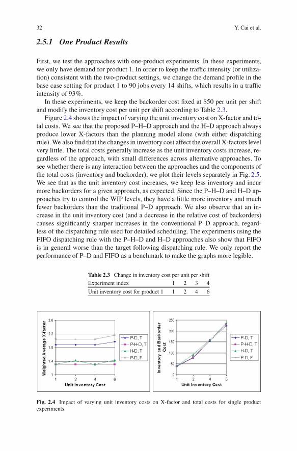
First, we test the approaches with one-product experiments. In these experiments,we only have demand for product 1. In order to keep the traffic intensity (or utiliza-tion) consistent with the two-product settings, we change the demand profile in thebase case setting for product 1 to 90 jobs every 14 shifts, which results in a trafficintensity of 93%.

In these experiments, we keep the backorder cost fixed at $50 per unit per shiftand modify the inventory cost per unit per shift according to Table 2.3.

Figure 2.4 shows the impact of varying the unit inventory cost on X-factor and to-tal costs. We see that the proposed P–H–D approach and the H–D approach alwaysproduce lower X-factors than the planning model alone (with either dispatchingrule). We also find that the changes in inventory cost affect the overall X-factors levelvery little. The total costs generally increase as the unit inventory costs increase, re-gardless of the approach, with small differences across alternative approaches. Tosee whether there is any interaction between the approaches and the components ofthe total costs (inventory and backorder), we plot their levels separately in Fig. 2.5.We see that as the unit inventory cost increases, we keep less inventory and incurmore backorders for a given approach, as expected. Since the P–H–D and H–D ap-proaches try to control the WIP levels, they have a little more inventory and muchfewer backorders than the traditional P–D approach. We also observe that an in-crease in the unit inventory cost (and a decrease in the relative cost of backorders)causes significantly sharper increases in the conventional P–D approach, regard-less of the dispatching rule used for detailed scheduling. The experiments using theFIFO dispatching rule with the P–H–D and H–D approaches also show that FIFOis in general worse than the target following dispatching rule. We only report theperformance of P–D and FIFO as a benchmark to make the graphs more legible.

Table 2.3 Change in inventory cost per unit per shift

Experiment index 1 2 3 4

Unit inventory cost for product 1 1 2 4 6

Fig. 2.4 Impact of varying unit inventory costs on X-factor and total costs for single productexperiments


Fig. 2.5 Impact on inventory and backorder quantity of inventory cost change for single product

Table 2.4 Demand distributions for the single product experiments

Experiment index 1 2 3 4

Demand (Uniform) 90 (88, 93) (85, 95) (83, 98)

Fig. 2.6 Impact on X-factor and cost of demand variance

2.5.1.1 Demand Variation

In actual manufacturing systems, demand may vary over time. This is especially truein the semiconductor industry, where the technology evolves so fast that it affectsthe demand levels for different categories of products differently. In the experimentsin this section, we modify the variability of the demand. Hence, for each week,we generate a random demand value drawn from a discrete uniform distribution.We change variability of demand over time by extending the underlying range ofthe distribution as shown in Table 2.4.

Again, as seen in Fig. 2.6, the X-factors obtained by P–H–D and H–D are muchlower than those obtained by P–D, regardless of the dispatching rule used with P–D.The H–D approach achieves the lowest total costs among the approaches tested.From these results, we see that increase in demand variation does not cause a signif-icant increase in the X-factor levels for a given planning/scheduling approach, whilethe increase in total costs can be high, especially for P–D and P–H–D.

34 Y. Cai et al.

Fig. 2.7 Impact of demand variation on inventory and backorder quantities

Figure 2.7 shows the average inventory and backorder level. We find that thebackorder level of the P–D approach increases much more sharply than in the otherapproaches as the demand variation increases, regardless of the dispatching ruleused in conjunction with it. Since the P–H–D approach obtains the implied demandprofile from planning and does not directly consider the original demand profile, itcannot perform well in controlling backorders as the demand variation increases.Although the P–H–D approach has higher backorder levels than the H–D approach,it has lower backorders than the P–D approach in three out of four experiments, anda comparable backorder level for the other one. However, the demand variation al-most has no impact on the H–D approach; the inventory and backorder levels do notclimb significantly while the demand variation increases. The reason could be thatthe H–D approach takes the original demand (and its variation) into account directlyand, to some extent, anticipates the variations in demand. Thus, it performs betterthan the alternatives in the case where the demand variation is a dominating factor.

2.5.2 Two Product Results

We now present the results of the two-product experiments. Since the two productscompete for capacity in this setting, the analysis is not straightforward. However,we still find some useful insights here.

2.5.2.1 Unit Inventory Cost

In this set of experiments, we evaluate the impact of varying unit inventory cost,which takes a value of $1, $2, $4, or $6 per job per shift. When we change theinventory cost for one product, we fix the inventory cost for the other to the baselevel, $1 per job per shift. The changes are displayed in Table 2.5.

Figures 2.8 and 2.9 show the simulation results of these experiments varying unitinventory cost for product 1 and for that of product 2, respectively.


Table 2.5 Inventory cost per unit per shift

Experiment 1 2 3 4 5 6 7

Inventory cost for product 1 1 2 4 6 1 1 1Inventory cost for product 2 1 1 1 1 2 4 6

Fig. 2.8 Impact of unit inventory cost of product 1

Fig. 2.9 Impact of unit inventory cost of product 2

As before, increasing unit inventory costs results in increasing total costs andrelatively stable X-factor values for the tested approach. Comparing the differ-ent planning/scheduling approaches, the P–D approach with FIFO has the largestweighted average X-factor, and the P–D approach with target following the secondlargest. In general, the P–D approach with either dispatching rule has lower totalcosts, and the approaches with high level scheduling (P–H–D and H–D) have largertotal costs. For all the experiments in which we modified the unit inventory costfor product 1, the weighted average X-factors are similar for the P–H–D and H–Dapproach. Overall, P–H–D and H–D are the best in terms of the X-factor and theyare comparable to P–D with FIFO or target following dispatching.

2.5.2.2 Demand Variation

In the previous 2-product experiments, we have demand levels constant over time,at 55 units and 44 units per 14 shifts for products 1 and 2, respectively. To make it

36 Y. Cai et al.

more realistic, we change shift demands over time, setting the means to the levels inthe constant demand case. The distributions used to create individual shift demandlevels are discrete uniform as in the one product experiment. We change the demandvariation by extending the range of the uniform distribution, taking range values of0 (no variation, fixed demand scenario), 5, 10, or 15. For example, when we setthe variation range to 5, the demand distribution is discrete uniform between 53and 58 (both inclusive, represented by Uniform(53, 58)) for product 1, and Uniform(42, 47) for product 2. These levels are described in Table 2.6.

Figures 2.10 and 2.11 show the impact of demand variation of product 1 and 2,respectively. Again, we have lower weighted X-factors in the P–H–D approach andthe H–D approach. For the planning model, the cost increases when the demandvariation increases for the first product. As in the one product case, it seems that thehigh level scheduling approach is robust with respect to the demand variation.

Table 2.6 Demand profiles with different distributions

Experiment 1 2 3 4 5 6 7

Product 1 demand (Uniform) 55 (53, 58) (50, 60) (45, 61) 55 55 55Product 2 demand (Uniform) 44 44 44 44 (41, 47) (38, 50) (34, 53)

Fig. 2.10 Impact from demand variation of product 1

Fig. 2.11 Impact from demand variation of product 2


2.5.2.3 Machine Breakdowns

In the base experimental setting, described in Sect. 2.4.1, the time between machinefailures and the time to repair follow exponential distributions. The mean time be-tween failures (MTBF) at station 1 is 42 h, and the mean time to repair (MTTR)is 45 min, which produces an availability of 98.2% (long-term percentage of “up”time out of total time, i.e., MTBF/(MTBF+MTTR)). In this section, we evaluate theimpact of varying levels of machine breakdowns. However, to keep the evaluationsimple, we keep the traffic intensity of station 1 less than that of station 3, so thatthe bottleneck station does not change when we vary the downtime parameters. Asbefore, when we modify one of the factors we keep the others at the base levels.

We first vary the mean time between failures at station 1, and keep the meanrepair time at 45 min. The MTBF changes according to Table 2.7.

Figure 2.12 shows the impact of different mean times between failures at station 1on the weighted average X-factors for the tested planning/scheduling approaches. Inthese experiments, the P–H–D approach produces the lowest weighted X-factor, andits cost is comparable to the cost of the planning model. Although the H–D approachhas a slightly higher weighted X-factor than P–H–D (still lower than P–D with FIFOor target following), it has lower total costs than the other three approaches whenbreakdowns are more frequent. As the mean time between failures increases (i.e.,as the availability increases), the differences among the total cost of the variousapproaches decrease. Also, the weighted X-factor decreases as the disruptions areless frequent for all four approaches. Again, the FIFO dispatching rule with theplanning model gives the worst performance.

As part of the experiments in this section, we also vary the MTTR at station1 according to the values in Table 2.8. By keeping the MTBF at 42 h, we gener-ate availability levels comparable to those in the MTTR experiments. Figure 2.13

Table 2.7 Mean times between failures at station 1

MTBF (h) 7.5 9 12.5 25 42

Station 1 availability 90% 91.6% 94% 97% 98.2%Station 1 traffic intensity 0.87 0.85 0.83 0.81 0.8

Fig. 2.12 Effect of mean time between failures at station 1

38 Y. Cai et al.

Table 2.8 Mean times to repair at station 1

MTTR(min) 252 210 150 75 45

Station 1 availability 90% 91.6% 94% 97% 98.2%Station 1 traffic intensity 0.87 0.85 0.83 0.81 0.8

Fig. 2.13 Impact to weighted average X-factor and cost from mean repair time at station 1

shows the effect of different mean repair times on X-factor and total costs. In theseexperiments, the approaches with high-level scheduling (P–H–D and H–D, bothwith target following dispatching) produce lower weighted X-factors than P–Dwith FIFO and target following. Again, P–H–D and H–D have similar weightedX-factors. In total costs, these approaches yield lower values than the planning-only-based approaches (P–D), especially when the repair times are long and availabilityis low. Comparing this with the previous set of experiments, we find that the impactfrom the breakdown duration (MTTR experiments) is more pronounced than theimpact from the frequency of breakdowns (MTBF experiments).

2.5.3 Gantt Chart Analysis

To analyze why P–H–D or H–D works better than P–D, we examine the Gantt chartsrepresenting the processing of jobs in some of the above experiments. As mentionedbefore, we choose the same random seed for all three approaches so that they seethe same realization of machine breakdowns. Figures 2.14 and 2.15 are two typicaltime periods in one replication of the same setting, which corresponds to the secondcolumn in Table 2.7.

As we can see from Fig. 2.14, in the P–D approach, during the 1.05–1.08 (�104)min time interval, there are no new releases. Therefore, when the machine breaksdown at station 1 around 1:12 � 104 min, there is not enough WIP at the bottleneckstation 3, and the station becomes idle at around 1:13 � 104 min. However, forthe P–H–D and H–D approach, the same disruption does not affect the bottleneckstation at all.

In Fig. 2.15, although the machine break down in station 1 affects the bottleneckstation in all three approaches, we can see clearly that the idle time of the bottleneckstation in the P–H–D and H–D approaches is significantly smaller than the one


Fig. 2.14 Gantt chart for three approaches between 0.9 and 1.3 (�104) min

in the P–D approach. If we look at the Gantt chart along the whole time horizon,we find that situations such as those seen in Figs. 2.14 and 2.15 are very common.In the P–H–D and H–D approaches, jobs are “pushed” to the bottleneck station,thus some jobs can avoid the machine-break-down situation without being held atstation 1. On the contrary, the total number of jobs released is almost the same forall three approaches since the demand profiles are the same. Therefore, the weightedaverage cycle times in the P–H–D and H–D approach are smaller than the cycle timeachieved by the P–D approach.

40 Y. Cai et al.

Fig. 2.15 Gantt chart for three approaches between 2 and 2.3 (�104)min

2.6 Summary

Production planning is a critical process for every manufacturing company since itdirectly affects the performance of detailed scheduling, which ultimately determinesthe overall performance of the manufacturing system. Despite this interdependency,in many manufacturing companies planning and detailed scheduling activities areseparated, with a limited coordination between them. Usually, planning decisions


obtained from a long-term model are fed into a scheduling model as restrictions,jobs to be released, and due dates. Detailed scheduling is typically handled throughdispatching.

In this paper, we suggest incorporating an intermediate stage into the usualplanning-scheduling hierarchy to seek coordination between planning and detailedscheduling. This approach consists of the usual planning model and a high levelscheduling model, both of which feed dispatching-based detailed scheduling. Thehigh level scheduling model explicitly controls the WIP over time at each stagein the system, thus providing a more specific guide to detailed scheduling. Ournumerical results indicate that the proposed approach results in shorter cycle times(realized as a lower weighted X-factor) than the conventional two-stage approach offeeding planning results into a detailed scheduling algorithm. In most cases, the useof the high level scheduling model, either as an intermediate step between planningand detailed scheduling or as an initial step before detailed scheduling, results inlower inventory and backorder costs. This approach without a major planning stepturns out to be especially suitable for situations with high demand variability. Allthese results indicate that if we consider more scheduling details in the planninglevel and/or at an intermediate level before detailed scheduling, we would havebetter performance on the shop-floor in terms of both cycle times and system costsincluding inventory and backorders.

In actual manufacturing systems, all planning and scheduling systems areimplemented in a rolling horizon fashion. This is also true for the three-levelplanning=high-level scheduling=detailed scheduling approach. For example, theplanning model would generate a plan for one quarter every month, and producethe first several months’ demand profile, release schedule, and production targets,for the upcoming weeks. This information would then be released to the high levelscheduling model. Then the high level scheduling model would generate a moregranular (say by day or shift) release policy and processing targets, for each majorprocessing step pertaining to the upcoming week or month. The detailed schedulingstep would try to implement the high-level scheduling decisions made for the nextfew days on the shop floor. High level scheduling and planning steps can be rerunwith some regular frequency (say every week and month, respectively). Duringthe execution of detailed scheduling, the current system status, such as WIP level,machine availability, may provide feedback that would initiate more frequent runsof the high level scheduling and planning models. We believe the rolling horizonapproach would improve the performance of the proposed approach that incorpo-rates a high-level scheduling model. Simulation of such a rolling horizon approachrequires significant effort and we leave this as a topic for future research.

References

Asmundsson J, Rardin R, Uzsoy R (2006) Tractable nonlinear production planning models forsemiconductor wafer fabrication facilities. IEEE Trans Semicond Manuf 19:95–111

Bertsimas D, Gamarnik D, Sethuraman J (2003) From fluid relaxation to practical algorithms forjob shop scheduling: the holding cost objective. Oper Res 51(5):798–813

42 Y. Cai et al.

Dai J, Weiss G (2002) A fluid heuristic for minimizing makespan in job shops. Oper Res50(4):692–707

Graves S (1986) A tactical planning model for a job shop. Oper Res 34:552–533Hackman S, Leachman R (1989) A general framework for modeling production. Manag Sci

35:478–495Horiguchi K, Raghavan N, Uzsoy R, Venkateswaran S (2001) Finite-capacity production planning

algorithms for a semiconductor wafer fabrication facility. Int J Prod Res 39:825–842Hung YF and Leachman RC (1996) A production planning methodology for semiconductor man-

ufacturing based on iterative simulation and linear programming calculations. IEEE TransSemicond Manuf 9(2):257–269

Jaikumar R (1974) An operational optimization procedure for production scheduling. ComputOper Res 1:191–200

Kim S, Yea S, Kim B (2003) Shift scheduling for steppers in the semiconductor wafer fabricationprocess. IIE Trans 34:167–177

Kleindorfer PR, Kriebel CH, Thompson GL, Kleindorfer GB (1975) Discrete optimal control ofproduction plains. Manag Sci 22

Leachman R, Kang J, Lin V (2002) SLIM: Short cycle time and low inventory in manufacturing atsamsung electronics. Interfaces 32(1):61–77

Lee Y, Kim T (2002) Manufacturing cycle time reduction using balance control in the semicon-ductor fabrication line. Prod Plann Contr 13:529–540

Missbauer H (2002) Aggregate order release planning for time-varying demand. Int J Prod Res40(3):699–718

Pahl J, Voˇ S, Woodruff D (2005) Production planning with load dependent lead times. Q J OperRes 3:257–302

Qin SJ and Badgwell TA (2003) A survey of industrial model predictive control technology. ContrEng Practice 11:733–764

Rose O (2002) Some issues of the critical ratio dispatch rule in semiconductor manufacturing.Proceedings of the 2002 Winter Simulation Conference, December 2002

Tsakalis K, Godoy JF, Rodriguez A (2003) Hierarchical modeling and control for re-entrant semi-conductor fabrication lines: A mini-fab benchmark. pp. 578–587

Vargas-Villami F, Rivera D (2000) Multilayer optimization and scheduling using model predic-tive control: application to reentrant semiconductor manufacturing lines. Comput Chem Eng24:2009–2021

Vargas-Villami F, Rivera D, Kempf K (2003) A hierarchical approach to production control ofreentrant semiconductor manufacturing lines. IEEE Trans Contr Syst Technol 11(4):578–587

http://www.springer.com/978-1-4419-8190-5

chapter 2 production planning and scheduling: interaction ... · pdf file2 production planning...

Documents