1 aggregate planning. 2 master scheduling material requirements planning order scheduling weekly...
TRANSCRIPT
1
Aggregate Planning
2
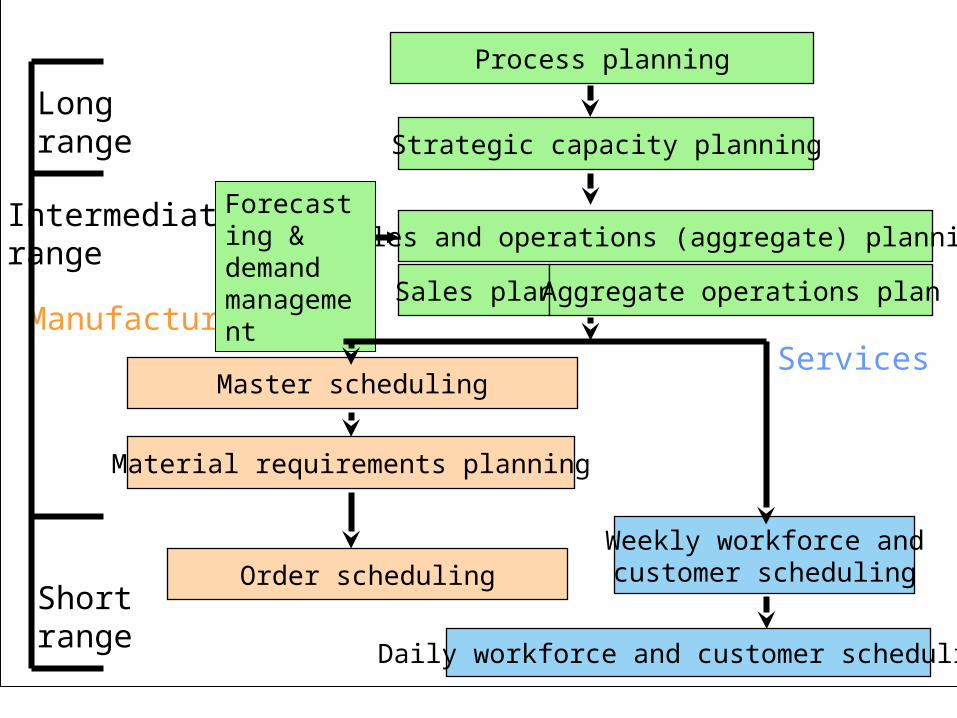
Master scheduling
Material requirements planning
Order schedulingWeekly workforce andcustomer scheduling
Daily workforce and customer scheduling
Process planning
Strategic capacity planning
Sales and operations (aggregate) planning
Longrange
Intermediaterange
Shortrange
ManufacturingServices
Sales plan Aggregate operations plan
Forecasting & demand management
3
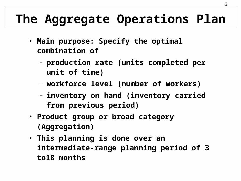
The Aggregate Operations Plan
• Main purpose: Specify the optimal combination of– production rate (units completed per unit of
time)– workforce level (number of workers)– inventory on hand (inventory carried from
previous period)• Product group or broad category (Aggregation)• This planning is done over an intermediate-range
planning period of 3 to18 months

4
Required Inputs to the Production Planning System
Planning for
production
External capacity
Competitors’behavior
Raw material availability
Market demand
Economic conditions
Currentphysical capacity
Current workforce
Inventory levels
Activities required for production
External to firm
Internal to firm
5
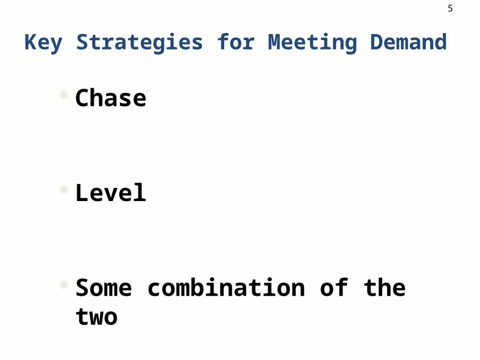
Key Strategies for Meeting Demand
Chase
Level
Some combination of the two
6
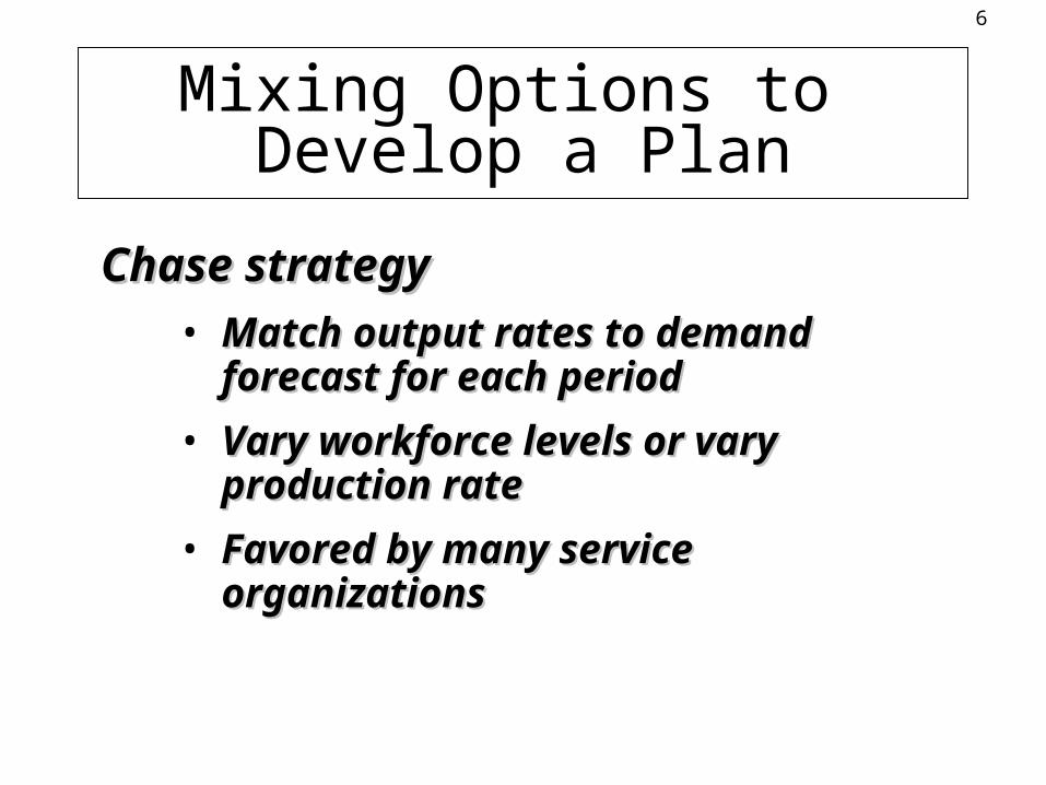
Mixing Options to Develop a Plan
Chase strategyChase strategy• Match output rates to demand Match output rates to demand
forecast for each periodforecast for each period
• Vary workforce levels or vary Vary workforce levels or vary production rateproduction rate
• Favored by many service Favored by many service organizationsorganizations
7
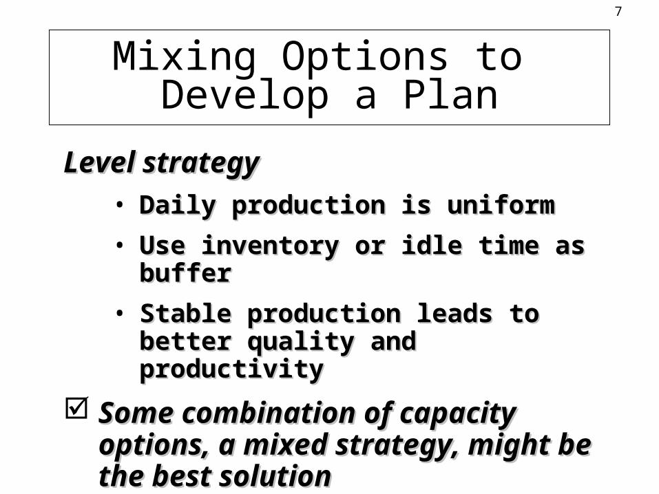
Level strategyLevel strategy• Daily production is uniformDaily production is uniform
• Use inventory or idle time as bufferUse inventory or idle time as buffer
• Stable production leads to better Stable production leads to better quality and productivityquality and productivity
Some combination of capacity Some combination of capacity options, a mixed strategy, might be options, a mixed strategy, might be the best solutionthe best solution
Mixing Options to Develop a Plan
8
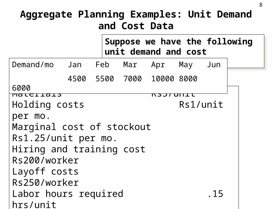
Aggregate Planning Examples: Unit Demand and Cost Data
Materials Rs5/unitHolding costs Rs1/unit per mo.Marginal cost of stockout Rs1.25/unit per mo.Hiring and training cost Rs200/workerLayoff costs Rs250/workerLabor hours required .15 hrs/unitStraight time labor cost Rs8/hourBeginning inventory 250 unitsProductive hours/worker/day 7.25Paid straight hrs/day 8
Suppose we have the following unit demand and cost information:
Suppose we have the following unit demand and cost information:
Demand/mo Jan Feb Mar Apr May Jun
4500 5500 7000 10000 8000 6000
9
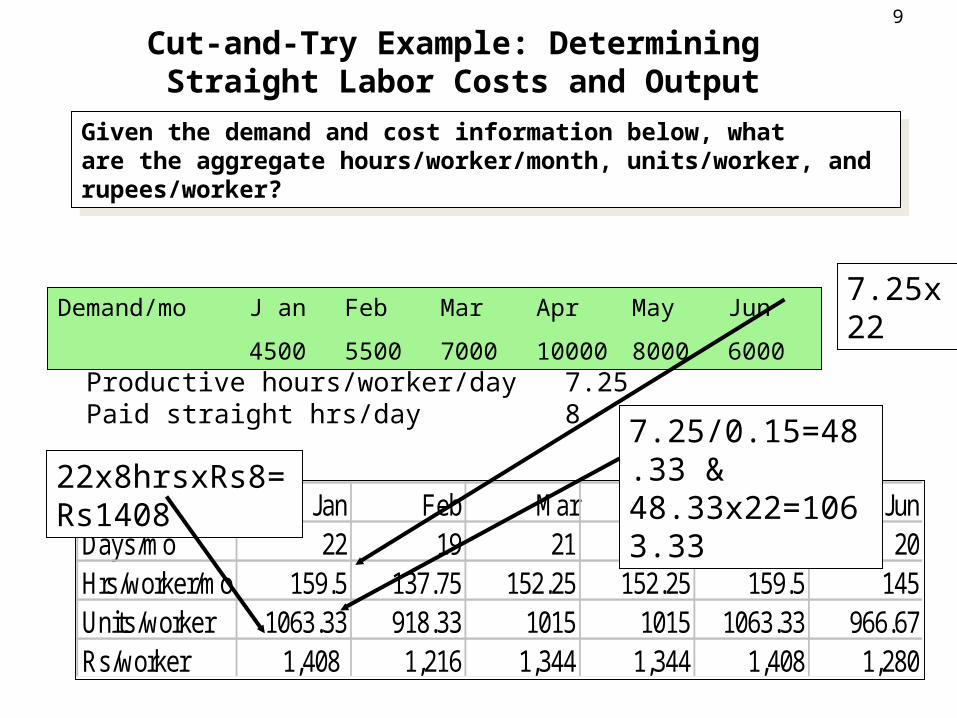
Jan Feb Mar Apr May JunDays/mo 22 19 21 21 22 20Hrs/worker/mo 159.5 137.75 152.25 152.25 159.5 145Units/worker 1063.33 918.33 1015 1015 1063.33 966.67Rs/worker 1,408 1,216 1,344 1,344 1,408 1,280
Productive hours/worker/day 7.25Paid straight hrs/day 8
Demand/mo J an Feb Mar Apr May Jun
4500 5500 7000 10000 8000 6000
Given the demand and cost information below, whatare the aggregate hours/worker/month, units/worker, and rupees/worker?
Given the demand and cost information below, whatare the aggregate hours/worker/month, units/worker, and rupees/worker?
7.25x22
7.25/0.15=48.33 & 48.33x22=1063.3322x8hrsxRs8=Rs1
408
Cut-and-Try Example: Determining Straight Labor Costs and Output
10
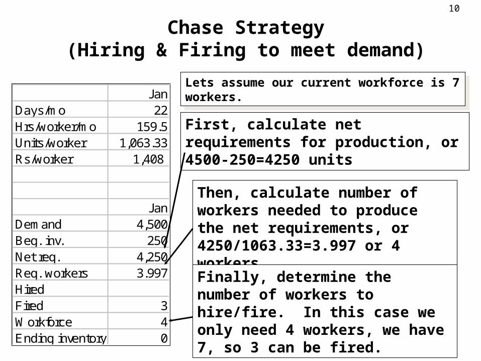
Chase Strategy(Hiring & Firing to meet demand)
JanDays/mo 22Hrs/worker/mo 159.5Units/worker 1,063.33Rs/worker 1,408
JanDemand 4,500Beg. inv. 250Net req. 4,250Req. workers 3.997HiredFired 3Workforce 4Ending inventory 0
Lets assume our current workforce is 7 workers.
Lets assume our current workforce is 7 workers.
First, calculate net requirements for production, or 4500-250=4250 units
Then, calculate number of workers needed to produce the net requirements, or 4250/1063.33=3.997 or 4 workers
Finally, determine the number of workers to hire/fire. In this case we only need 4 workers, we have 7, so 3 can be fired.
11
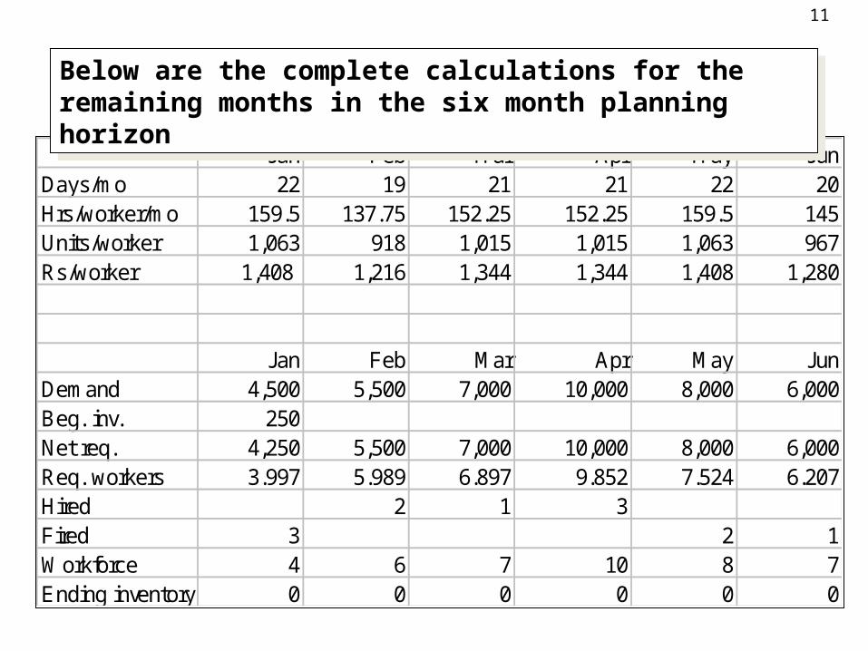
Jan Feb Mar Apr May JunDays/mo 22 19 21 21 22 20Hrs/worker/mo 159.5 137.75 152.25 152.25 159.5 145Units/worker 1,063 918 1,015 1,015 1,063 967Rs/worker 1,408 1,216 1,344 1,344 1,408 1,280
Jan Feb Mar Apr May JunDemand 4,500 5,500 7,000 10,000 8,000 6,000Beg. inv. 250Net req. 4,250 5,500 7,000 10,000 8,000 6,000Req. workers 3.997 5.989 6.897 9.852 7.524 6.207Hired 2 1 3Fired 3 2 1Workforce 4 6 7 10 8 7Ending inventory 0 0 0 0 0 0
Below are the complete calculations for the remaining months in the six month planning horizon
Below are the complete calculations for the remaining months in the six month planning horizon
12
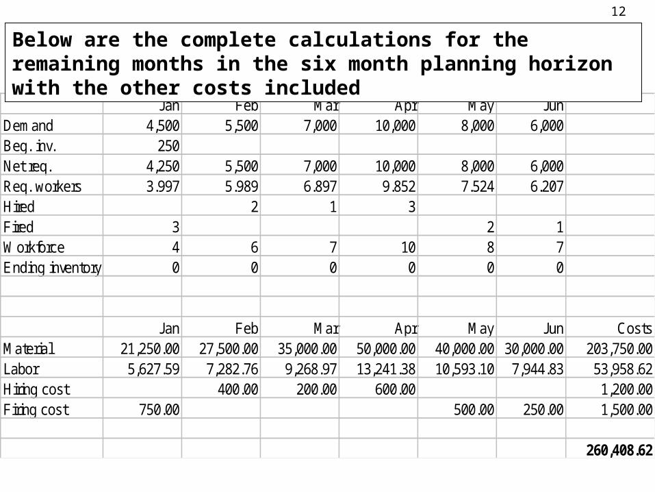
Jan Feb Mar Apr May JunDemand 4,500 5,500 7,000 10,000 8,000 6,000Beg. inv. 250Net req. 4,250 5,500 7,000 10,000 8,000 6,000Req. workers 3.997 5.989 6.897 9.852 7.524 6.207Hired 2 1 3Fired 3 2 1Workforce 4 6 7 10 8 7Ending inventory 0 0 0 0 0 0
Jan Feb Mar Apr May Jun CostsMaterial 21,250.00 27,500.00 35,000.00 50,000.00 40,000.00 30,000.00 203,750.00Labor 5,627.59 7,282.76 9,268.97 13,241.38 10,593.10 7,944.83 53,958.62Hiring cost 400.00 200.00 600.00 1,200.00Firing cost 750.00 500.00 250.00 1,500.00
260,408.62
Below are the complete calculations for the remaining months in the six month planning horizon with the other costs included
13
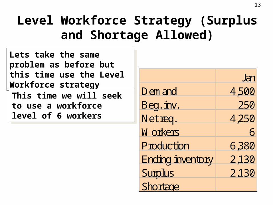
Level Workforce Strategy (Surplus and Shortage Allowed)
JanDemand 4,500Beg. inv. 250Net req. 4,250Workers 6Production 6,380Ending inventory 2,130Surplus 2,130Shortage
Lets take the same problem as before but this time use the Level Workforce strategy
Lets take the same problem as before but this time use the Level Workforce strategy
This time we will seek to use a workforce level of 6 workers
This time we will seek to use a workforce level of 6 workers
14
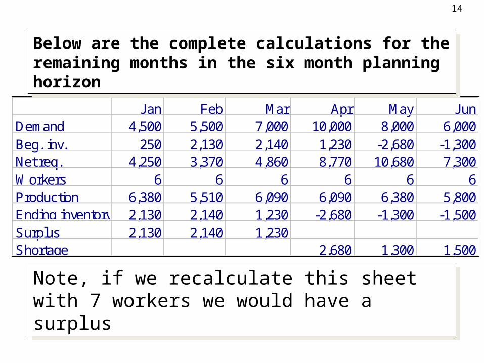
Jan Feb Mar Apr May JunDemand 4,500 5,500 7,000 10,000 8,000 6,000Beg. inv. 250 2,130 2,140 1,230 -2,680 -1,300Net req. 4,250 3,370 4,860 8,770 10,680 7,300Workers 6 6 6 6 6 6Production 6,380 5,510 6,090 6,090 6,380 5,800Ending inventory 2,130 2,140 1,230 -2,680 -1,300 -1,500Surplus 2,130 2,140 1,230Shortage 2,680 1,300 1,500
Note, if we recalculate this sheet with 7 workers we would have a surplus
Note, if we recalculate this sheet with 7 workers we would have a surplus
Below are the complete calculations for the remaining months in the six month planning horizon
Below are the complete calculations for the remaining months in the six month planning horizon
15
Jan Feb Mar Apr May Jun4,500 5,500 7,000 10,000 8,000 6,000
250 2,130 10 -910 -3,910 -1,6204,250 3,370 4,860 8,770 10,680 7,300
6 6 6 6 6 66,380 5,510 6,090 6,090 6,380 5,8002,130 2,140 1,230 -2,680 -1,300 -1,5002,130 2,140 1,230
2,680 1,300 1,500
Jan Feb Mar Apr May Jun8,448.00 7,296.00 8,064.00 8,064.00 8,448.00 7,680.00 48,000.00
31,900.00 27,550.00 30,450.00 30,450.00 31,900.00 29,000.00 181,250.002,130.00 2,140.00 1,230.00 5,500.00
3,350.00 1,625.00 1,875.00 6,850.00
241,600.00
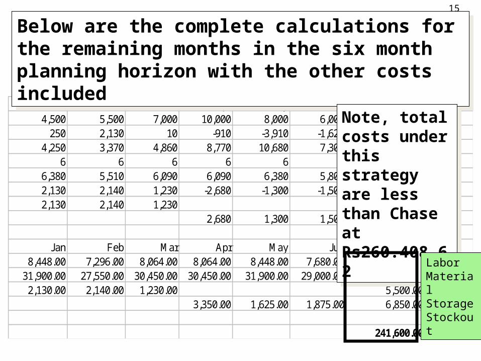
Below are the complete calculations for the remaining months in the six month planning horizon with the other costs included
Below are the complete calculations for the remaining months in the six month planning horizon with the other costs included
Note, total costs under this strategy are less than Chase at Rs260.408.62
Note, total costs under this strategy are less than Chase at Rs260.408.62
LaborMaterialStorageStockout
16
Chapter 15
Materials Requirements Planning
17
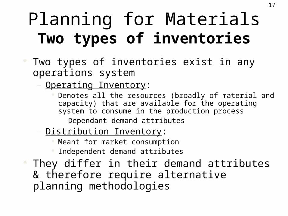
Planning for MaterialsTwo types of inventories
Two types of inventories exist in any operations system– Operating Inventory:
Denotes all the resources (broadly of material and capacity) that are available for the operating system to consume in the production process
Dependant demand attributes
– Distribution Inventory: Meant for market consumption Independent demand attributes
They differ in their demand attributes & therefore require alternative planning methodologies
18
Material Requirements PlanningDefined• Materials requirements planning (MRP) is a
means for determining the number of parts, components, and materials needed to produce a product
• MRP provides time scheduling information specifying when each of the materials, parts, and components should be ordered or produced
• Dependent demand drives MRP• MRP is a software system
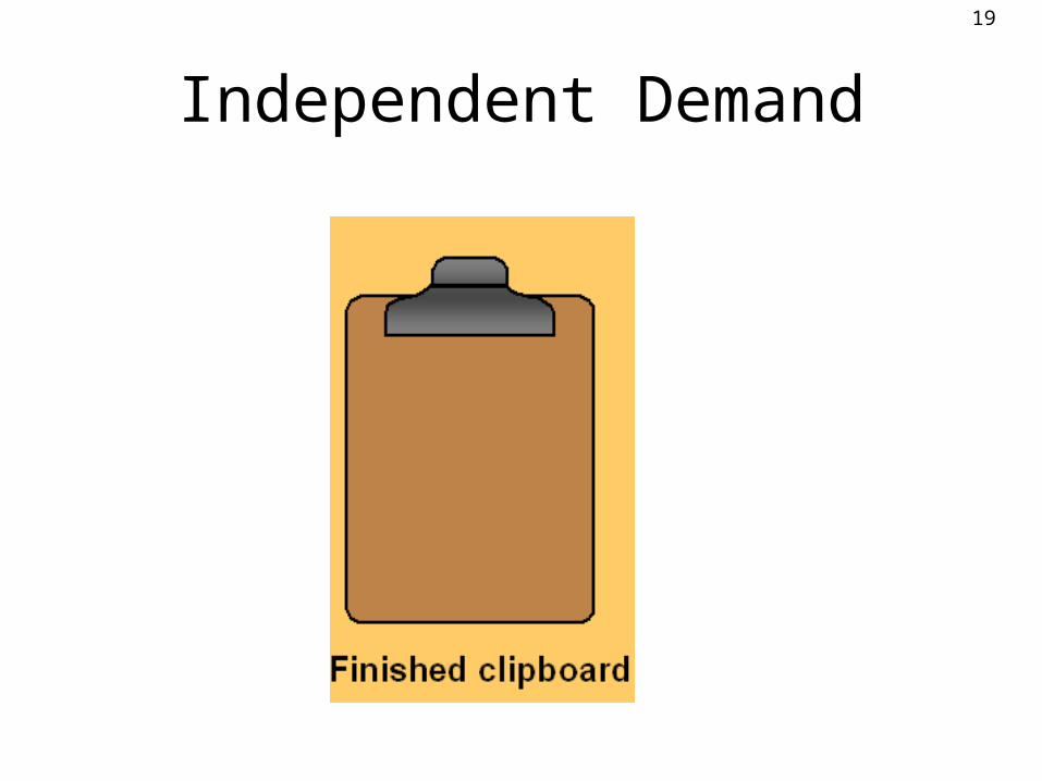
19
Independent Demand
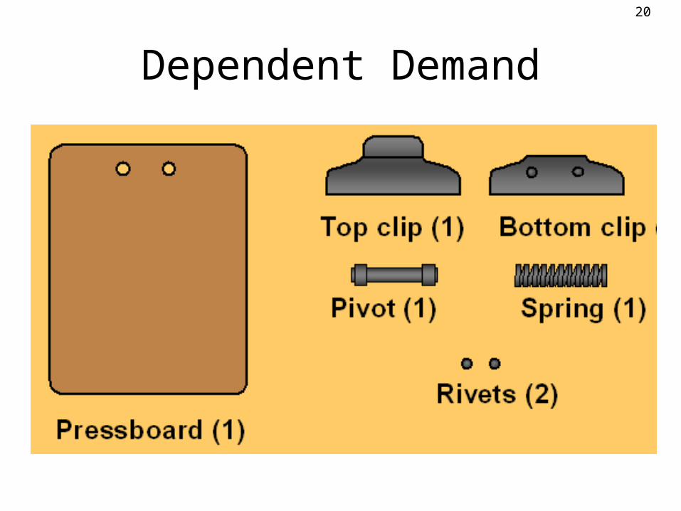
20
Dependent Demand
21
21
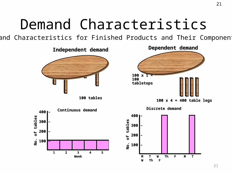
Demand Characteristics
11 22 33 44 55WeekWeek
400 400 –
300 300 –
200 200 –
100 100 –No
. o
f ta
ble
sN
o.
of
tab
les
Continuous demandContinuous demand
M T W Th F M T W Th FM T W Th F M T W Th F
400 400 –
300 300 –
200 200 –
100 100 –No
. o
f ta
ble
sN
o.
of
tab
les
Discrete demandDiscrete demand
Independent demandIndependent demand
100 tables100 tables
Dependent demandDependent demand
100 x 1 = 100 x 1 = 100 tabletops100 tabletops
100 x 4 = 400 table legs100 x 4 = 400 table legs
Demand Characteristics for Finished Products and Their Components
22
6
E(1)
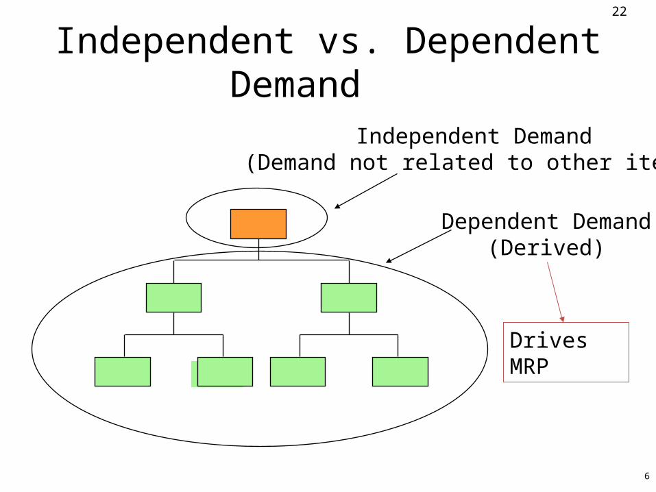
Independent vs. Dependent Demand
Independent Demand(Demand not related to other items)
Dependent Demand(Derived)
Drives MRP
23
23
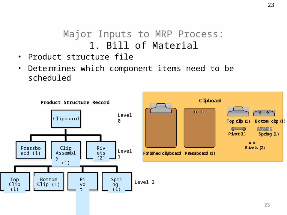
Major Inputs to MRP Process:1. Bill of Material
• Product structure file• Determines which component items need to be scheduled
Product Structure RecordProduct Structure Record
ClipboardLevel 0Level 0
Level 1Level 1
Level 2Level 2Spring (1)
Bottom Clip (1)
Top Clip (1)
Pivot (1)
Rivets (2)
Clip Assembly
(1)
Pressboard (1)
Top clip (1) Bottom clip (1)
Pivot (1) Spring (1)
Rivets (2)Finished clipboard Pressboard (1)
Clipboard

24
Example of MRP Logic and Product Structure Tree
B(4)
E(1)D(2)
C(2)
F(2)D(3)
A
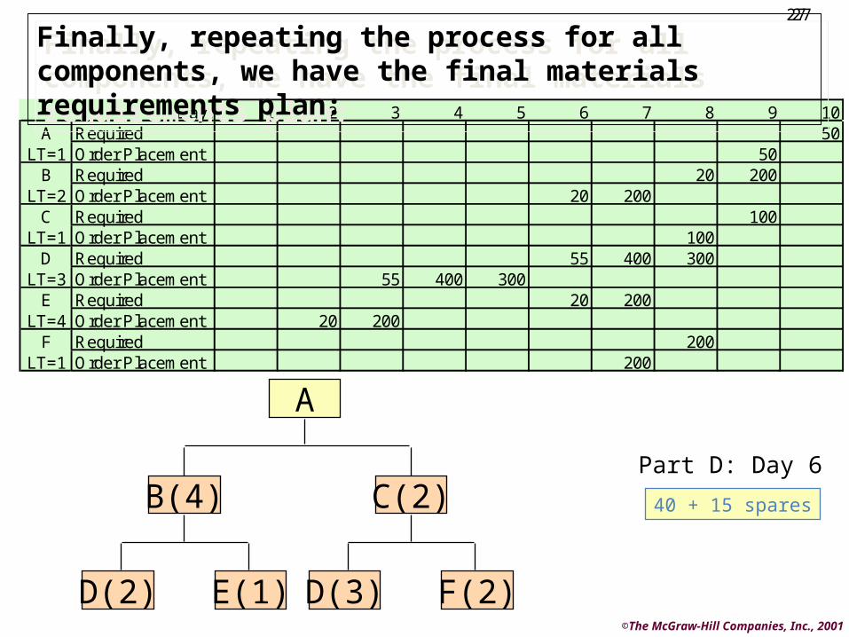
Product Structure Tree for Assembly A Lead TimesA 1 dayB 2 daysC 1 dayD 3 daysE 4 daysF 1 day
Total Unit DemandDay 10 50 ADay 8 20 B (Spares)Day 6 15 D (Spares)
Given the product structure tree for “A” and the lead time and demand information below, provide a materials requirements plan that defines the number of units of each component and when they will be needed
Given the product structure tree for “A” and the lead time and demand information below, provide a materials requirements plan that defines the number of units of each component and when they will be needed
25
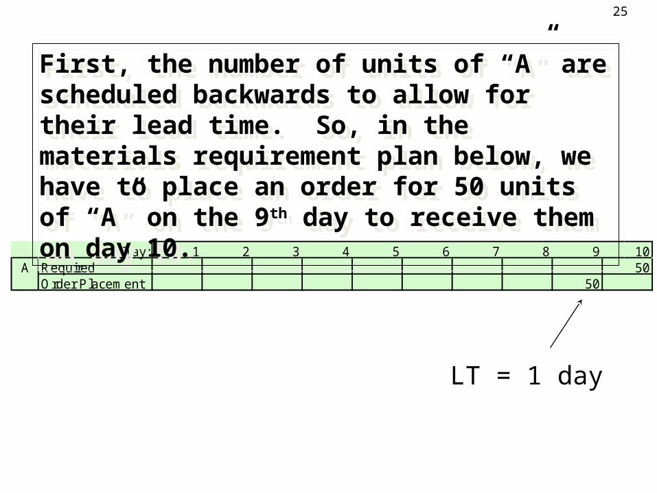
LT = 1 day
Day: 1 2 3 4 5 6 7 8 9 10A Required 50
Order Placement 50
First, the number of units of “A” are scheduled backwards to allow for their lead time. So, in the materials requirement plan below, we have to place an order for 50 units of “A” on the 9th day to receive them on day 10.
First, the number of units of “A” are scheduled backwards to allow for their lead time. So, in the materials requirement plan below, we have to place an order for 50 units of “A” on the 9th day to receive them on day 10.

26
Next, we need to start scheduling the components that make up “A”. In the case of component “B” we need 4 B’s for each A. Since we need 50 A’s, that means 200 B’s. And again, we back the schedule up for the necessary 2 days of lead time.
Next, we need to start scheduling the components that make up “A”. In the case of component “B” we need 4 B’s for each A. Since we need 50 A’s, that means 200 B’s. And again, we back the schedule up for the necessary 2 days of lead time.
Day: 1 2 3 4 5 6 7 8 9 10A Required 50
Order Placement 50B Required 20 200
Order Placement 20 200
B(4)
E(1)D(2)
C(2)
F(2)D(3)
A
SparesLT = 2
4x50=200
27
Day: 1 2 3 4 5 6 7 8 9 10A Required 50
LT=1 Order Placement 50B Required 20 200
LT=2 Order Placement 20 200C Required 100
LT=1 Order Placement 100D Required 55 400 300
LT=3 Order Placement 55 400 300E Required 20 200
LT=4 Order Placement 20 200F Required 200
LT=1 Order Placement 200
B(4)
E(1)D(2)
C(2)
F(2)D(3)
A
40 + 15 spares
Part D: Day 6
Finally, repeating the process for all components, we have the final materials requirements plan:
Finally, repeating the process for all components, we have the final materials requirements plan:
©The McGraw-Hill Companies, Inc., 2001
27
28
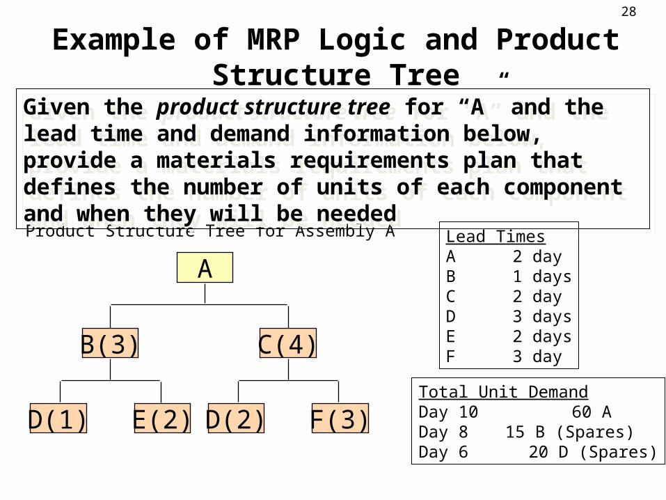
Example of MRP Logic and Product Structure Tree
B(3)
E(2)D(1)
C(4)
F(3)D(2)
A
Product Structure Tree for Assembly A Lead TimesA 2 dayB 1 daysC 2 dayD 3 daysE 2 daysF 3 day
Total Unit DemandDay 10 60 ADay 8 15 B (Spares)Day 6 20 D (Spares)
Given the product structure tree for “A” and the lead time and demand information below, provide a materials requirements plan that defines the number of units of each component and when they will be needed
Given the product structure tree for “A” and the lead time and demand information below, provide a materials requirements plan that defines the number of units of each component and when they will be needed
29
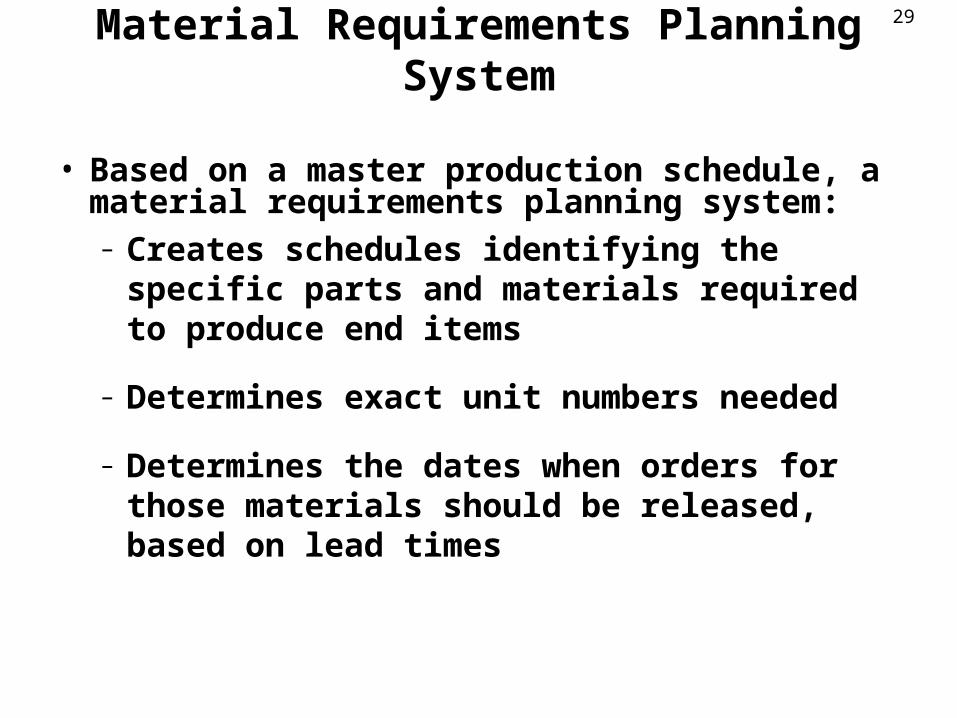
Material Requirements Planning System
• Based on a master production schedule, a material requirements planning system:– Creates schedules identifying the specific parts
and materials required to produce end items
– Determines exact unit numbers needed
– Determines the dates when orders for those materials should be released, based on lead times
3030
©The McGraw-Hill Companies, Inc., 2004
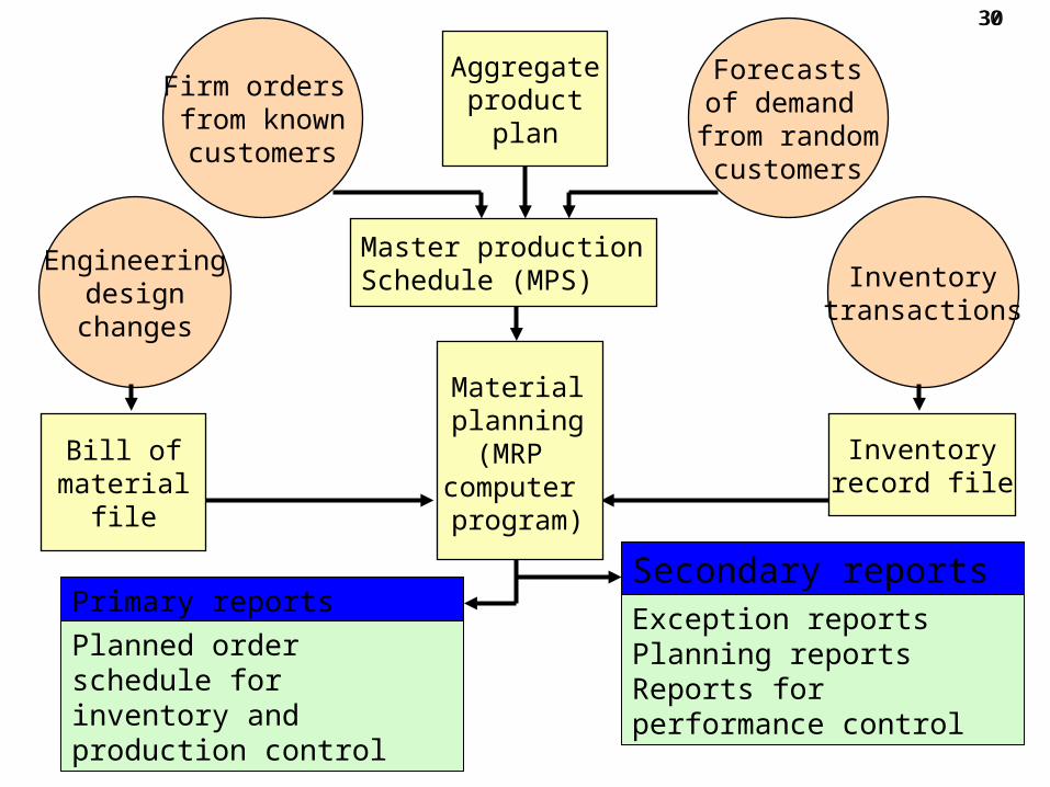
Firm orders from knowncustomers
Forecastsof demand
from randomcustomers
Aggregateproduct
plan
Bill ofmaterial
file
Engineeringdesign
changes
Inventoryrecord file
Inventorytransactions
Master productionSchedule (MPS)
Primary reportsSecondary reports
Planned order schedule for inventory and production control
Exception reportsPlanning reportsReports for performance control
Materialplanning(MRP
computer program)

31
Bill of Materials (BOM) FileA Complete Product Description
• Materials• Parts• Components• Production sequence • Modular BOM
– Subassemblies
• Super BOM– Fractional options

32
Inventory Records File
• Each inventory item carried as a separate file– Status according to “time buckets”
• Pegging– Identify each parent item that created demand
33
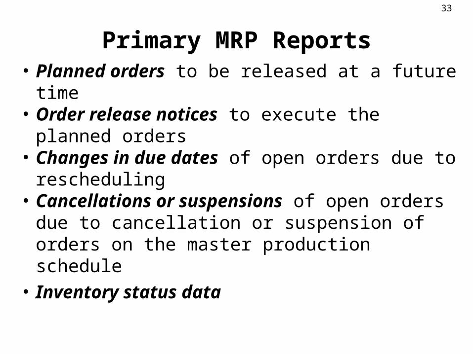
Primary MRP Reports• Planned orders to be released at a future time• Order release notices to execute the planned
orders• Changes in due dates of open orders due to
rescheduling • Cancellations or suspensions of open orders due
to cancellation or suspension of orders on the master production schedule
• Inventory status data
34
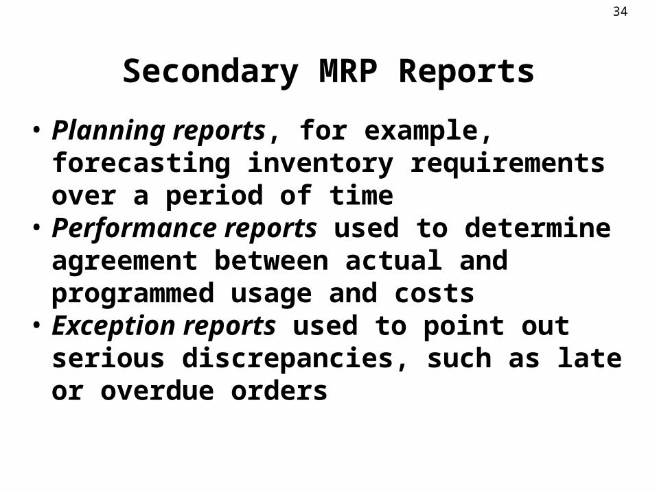
Secondary MRP Reports
• Planning reports, for example, forecasting inventory requirements over a period of time
• Performance reports used to determine agreement between actual and programmed usage and costs
• Exception reports used to point out serious discrepancies, such as late or overdue orders
35
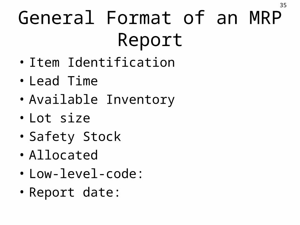
General Format of an MRP Report
• Item Identification• Lead Time• Available Inventory• Lot size• Safety Stock• Allocated• Low-level-code:• Report date:
36
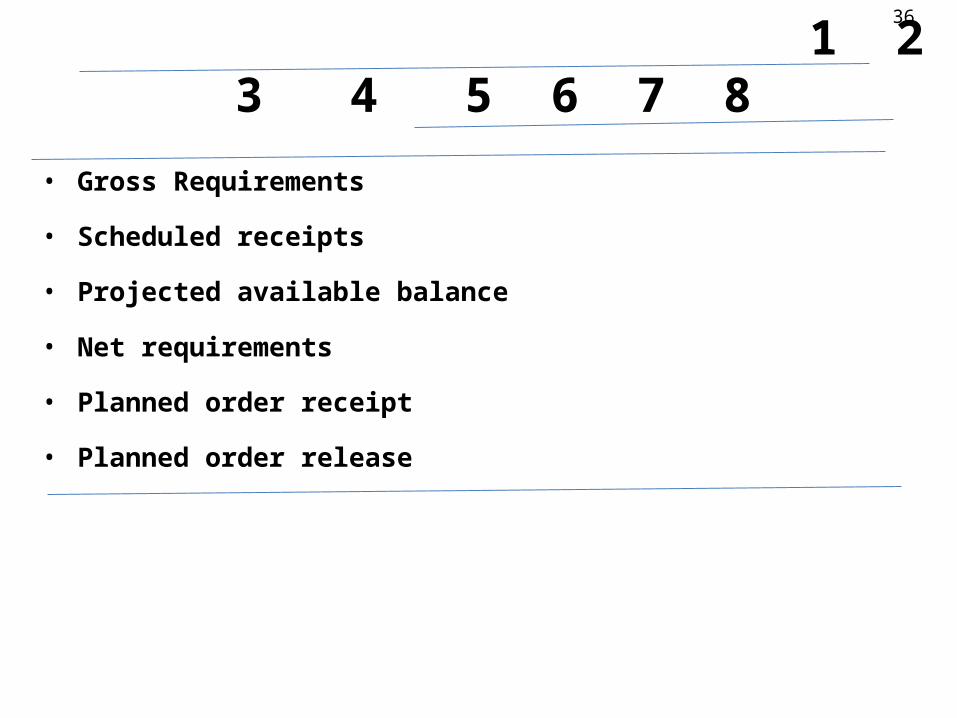
Period Week 1 2 3 4 5 6 7 8
• Gross Requirements
• Scheduled receipts
• Projected available balance
• Net requirements
• Planned order receipt
• Planned order release
37
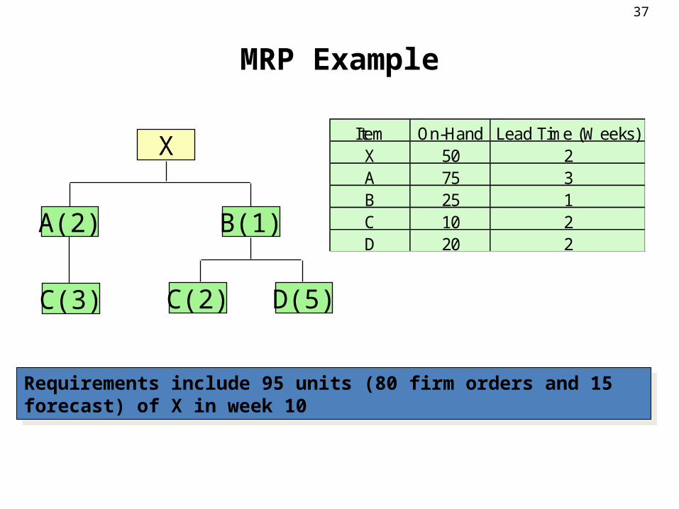
MRP Example
A(2) B(1)
D(5)C(2)
X
C(3)
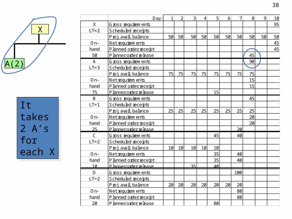
Item On-Hand Lead Time (Weeks)X 50 2A 75 3B 25 1C 10 2D 20 2
Requirements include 95 units (80 firm orders and 15 forecast) of X in week 10
Requirements include 95 units (80 firm orders and 15 forecast) of X in week 10
38
A(2)
X
Day: 1 2 3 4 5 6 7 8 9 10X Gross requirements 95
LT=2 Scheduled receipts Proj. avail. balance 50 50 50 50 50 50 50 50 50 50
On- Net requirements 45hand Planned order receipt 4550 Planner order release 45A Gross requirements 90
LT=3 Scheduled receipts Proj. avail. balance 75 75 75 75 75 75 75 75
On- Net requirements 15 hand Planned order receipt 15 75 Planner order release 15 B Gross requirements 45
LT=1 Scheduled receipts Proj. avail. balance 25 25 25 25 25 25 25 25
On- Net requirements 20 hand Planned order receipt 20 25 Planner order release 20 C Gross requirements 45 40
LT=2 Scheduled receipts Proj. avail. balance 10 10 10 10 10
On- Net requirements 35 40 hand Planned order receipt 35 40 10 Planner order release 35 40 D Gross requirements 100
LT=2 Scheduled receipts Proj. avail. balance 20 20 20 20 20 20 20
On- Net requirements 80 hand Planned order receipt 80 20 Planner order release 80
It takes 2 A’s for each X
It takes 2 A’s for each X
39
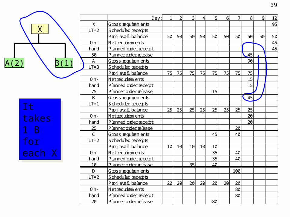
Day: 1 2 3 4 5 6 7 8 9 10X Gross requirements 95
LT=2 Scheduled receipts Proj. avail. balance 50 50 50 50 50 50 50 50 50 50
On- Net requirements 45hand Planned order receipt 4550 Planner order release 45A Gross requirements 90
LT=3 Scheduled receipts Proj. avail. balance 75 75 75 75 75 75 75 75
On- Net requirements 15 hand Planned order receipt 15 75 Planner order release 15 B Gross requirements 45
LT=1 Scheduled receipts Proj. avail. balance 25 25 25 25 25 25 25 25
On- Net requirements 20 hand Planned order receipt 20 25 Planner order release 20 C Gross requirements 45 40
LT=2 Scheduled receipts Proj. avail. balance 10 10 10 10 10
On- Net requirements 35 40 hand Planned order receipt 35 40 10 Planner order release 35 40 D Gross requirements 100
LT=2 Scheduled receipts Proj. avail. balance 20 20 20 20 20 20 20
On- Net requirements 80 hand Planned order receipt 80 20 Planner order release 80
B(1)A(2)
X
It takes 1 B for each X
It takes 1 B for each X
40
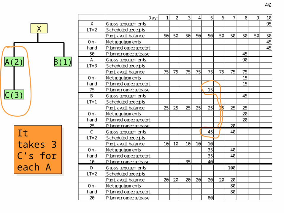
A(2) B(1)
X
C(3)
Day: 1 2 3 4 5 6 7 8 9 10X Gross requirements 95
LT=2 Scheduled receipts Proj. avail. balance 50 50 50 50 50 50 50 50 50 50
On- Net requirements 45hand Planned order receipt 4550 Planner order release 45A Gross requirements 90
LT=3 Scheduled receipts Proj. avail. balance 75 75 75 75 75 75 75 75
On- Net requirements 15 hand Planned order receipt 15 75 Planner order release 15 B Gross requirements 45
LT=1 Scheduled receipts Proj. avail. balance 25 25 25 25 25 25 25 25
On- Net requirements 20 hand Planned order receipt 20 25 Planner order release 20 C Gross requirements 45 40
LT=2 Scheduled receipts Proj. avail. balance 10 10 10 10 10
On- Net requirements 35 40 hand Planned order receipt 35 40 10 Planner order release 35 40 D Gross requirements 100
LT=2 Scheduled receipts Proj. avail. balance 20 20 20 20 20 20 20
On- Net requirements 80 hand Planned order receipt 80 20 Planner order release 80
It takes 3 C’s for each A
It takes 3 C’s for each A
41
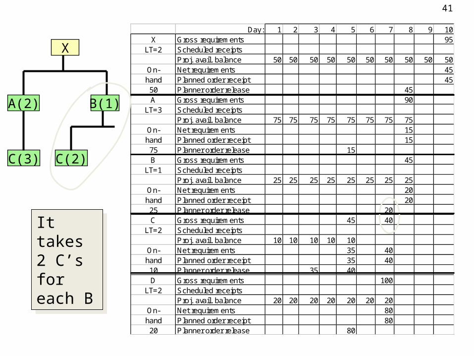
A(2) B(1)
C(2)
X
C(3)
Day: 1 2 3 4 5 6 7 8 9 10X Gross requirements 95
LT=2 Scheduled receipts Proj. avail. balance 50 50 50 50 50 50 50 50 50 50
On- Net requirements 45hand Planned order receipt 4550 Planner order release 45A Gross requirements 90
LT=3 Scheduled receipts Proj. avail. balance 75 75 75 75 75 75 75 75
On- Net requirements 15 hand Planned order receipt 15 75 Planner order release 15 B Gross requirements 45
LT=1 Scheduled receipts Proj. avail. balance 25 25 25 25 25 25 25 25
On- Net requirements 20 hand Planned order receipt 20 25 Planner order release 20 C Gross requirements 45 40
LT=2 Scheduled receipts Proj. avail. balance 10 10 10 10 10
On- Net requirements 35 40 hand Planned order receipt 35 40 10 Planner order release 35 40 D Gross requirements 100
LT=2 Scheduled receipts Proj. avail. balance 20 20 20 20 20 20 20
On- Net requirements 80 hand Planned order receipt 80 20 Planner order release 80
It takes 2 C’s for each B
It takes 2 C’s for each B
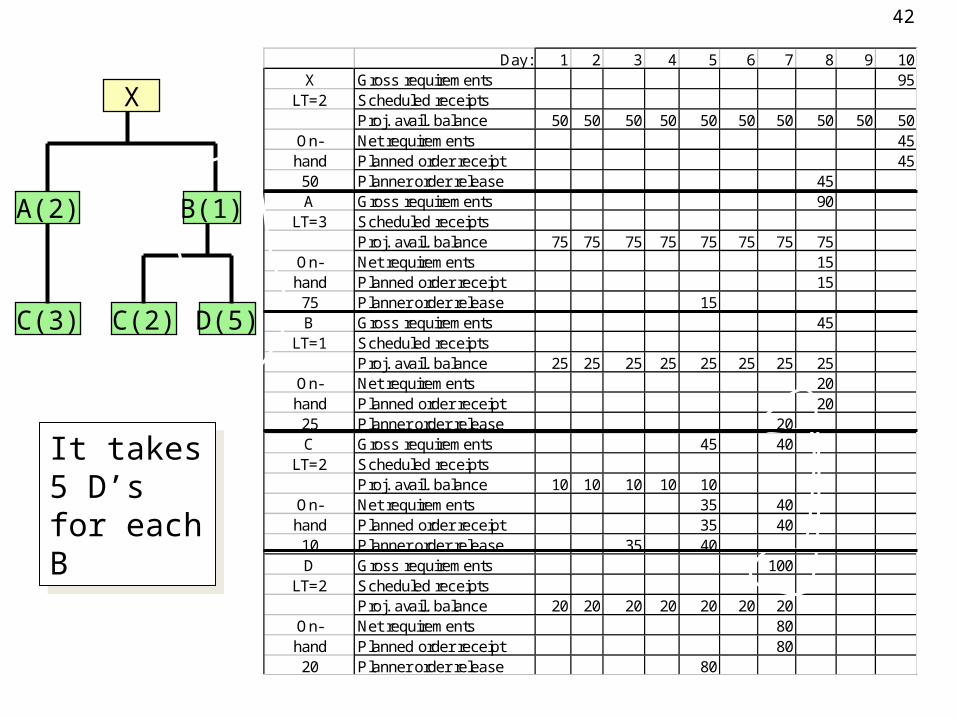
42
A(2) B(1)
D(5)C(2)
X
C(3)
Day: 1 2 3 4 5 6 7 8 9 10X Gross requirements 95
LT=2 Scheduled receipts Proj. avail. balance 50 50 50 50 50 50 50 50 50 50
On- Net requirements 45hand Planned order receipt 4550 Planner order release 45A Gross requirements 90
LT=3 Scheduled receipts Proj. avail. balance 75 75 75 75 75 75 75 75
On- Net requirements 15 hand Planned order receipt 15 75 Planner order release 15 B Gross requirements 45
LT=1 Scheduled receipts Proj. avail. balance 25 25 25 25 25 25 25 25
On- Net requirements 20 hand Planned order receipt 20 25 Planner order release 20 C Gross requirements 45 40
LT=2 Scheduled receipts Proj. avail. balance 10 10 10 10 10
On- Net requirements 35 40 hand Planned order receipt 35 40 10 Planner order release 35 40 D Gross requirements 100
LT=2 Scheduled receipts Proj. avail. balance 20 20 20 20 20 20 20
On- Net requirements 80 hand Planned order receipt 80 20 Planner order release 80
It takes 5 D’s for each B
It takes 5 D’s for each B
43
Calculation of Order Size in MRP
• Lot-for-lot Method
• EOQ Method
• Least Total Cost Method
• Least Unit Cost Method
44
Operation Scheduling
45
What is Scheduling?
• Last stage of planning before production occurs
• Specifies when labor, equipment, and facilities are needed to produce a product or provide a service
17-45
46
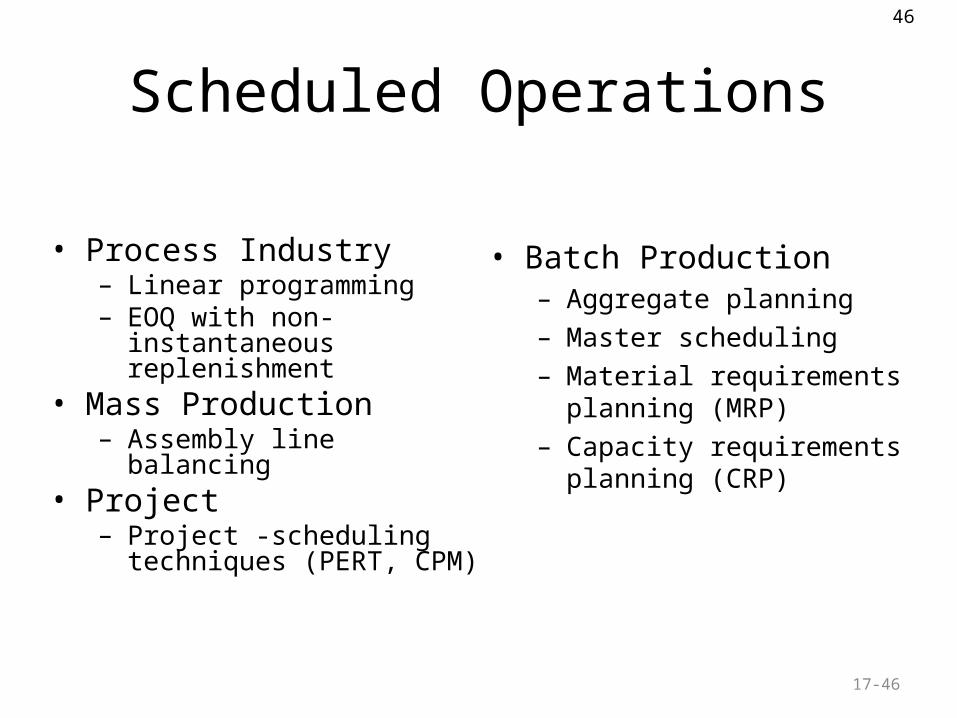
Scheduled Operations
• Process Industry– Linear programming– EOQ with non-instantaneous
replenishment• Mass Production
– Assembly line balancing• Project
– Project -scheduling techniques (PERT, CPM)
• Batch Production– Aggregate planning– Master scheduling– Material requirements
planning (MRP)– Capacity requirements
planning (CRP)
17-46
47
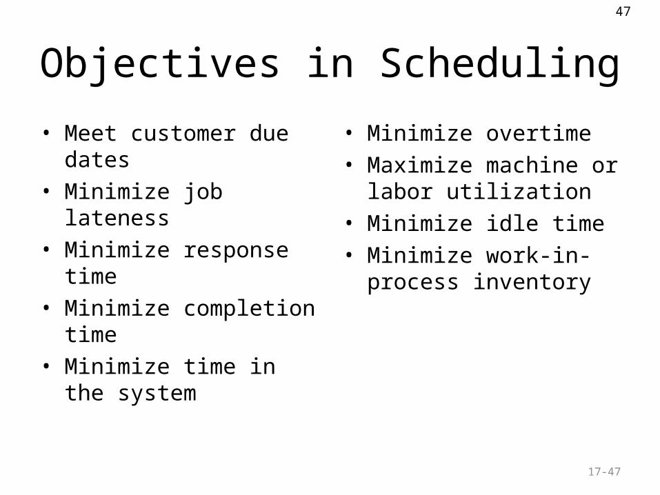
Objectives in Scheduling
• Meet customer due dates• Minimize job lateness• Minimize response time• Minimize completion time• Minimize time in the system
• Minimize overtime• Maximize machine or labor
utilization• Minimize idle time• Minimize work-in-process
inventory
17-47
48
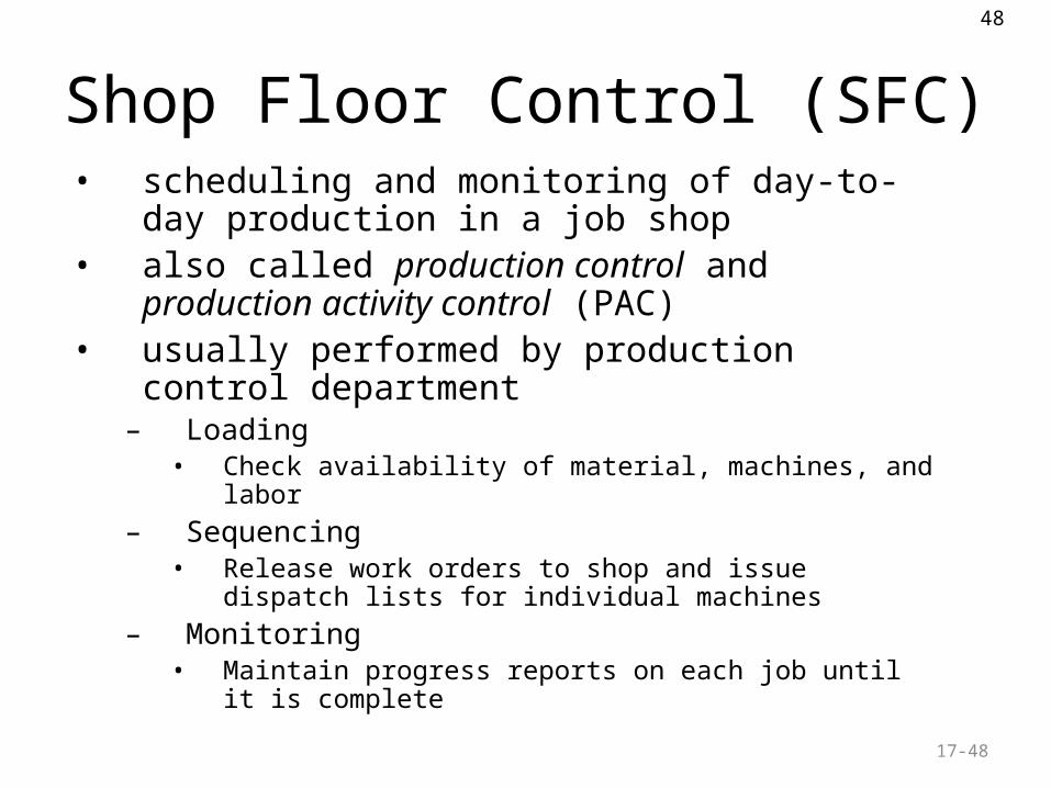
Shop Floor Control (SFC)• scheduling and monitoring of day-to-day production in a
job shop• also called production control and production activity
control (PAC)• usually performed by production control department
– Loading• Check availability of material, machines, and labor
– Sequencing• Release work orders to shop and issue dispatch lists for individual
machines– Monitoring
• Maintain progress reports on each job until it is complete
17-48
49
Loading
• Process of assigning work to limited resources• Perform work with most efficient resources• Use assignment method of linear
programming to determine allocation
17-49
50
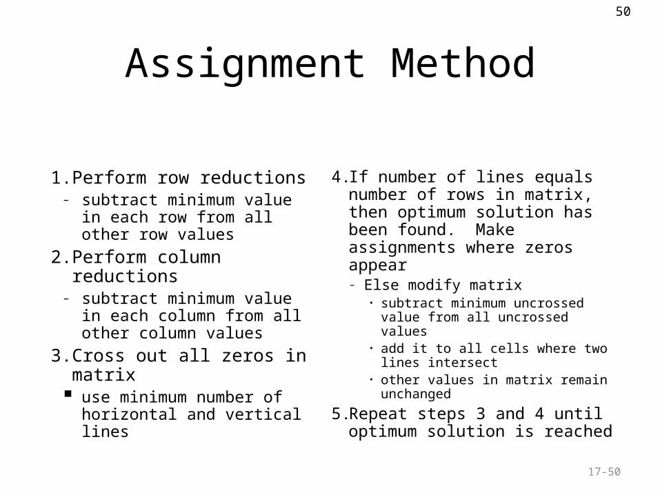
Assignment Method
1. Perform row reductions– subtract minimum value in each
row from all other row values2. Perform column reductions
– subtract minimum value in each column from all other column values
3. Cross out all zeros in matrix use minimum number of
horizontal and vertical lines
4. If number of lines equals number of rows in matrix, then optimum solution has been found. Make assignments where zeros appear– Else modify matrix
• subtract minimum uncrossed value from all uncrossed values
• add it to all cells where two lines intersect
• other values in matrix remain unchanged
5. Repeat steps 3 and 4 until optimum solution is reached
17-50
51
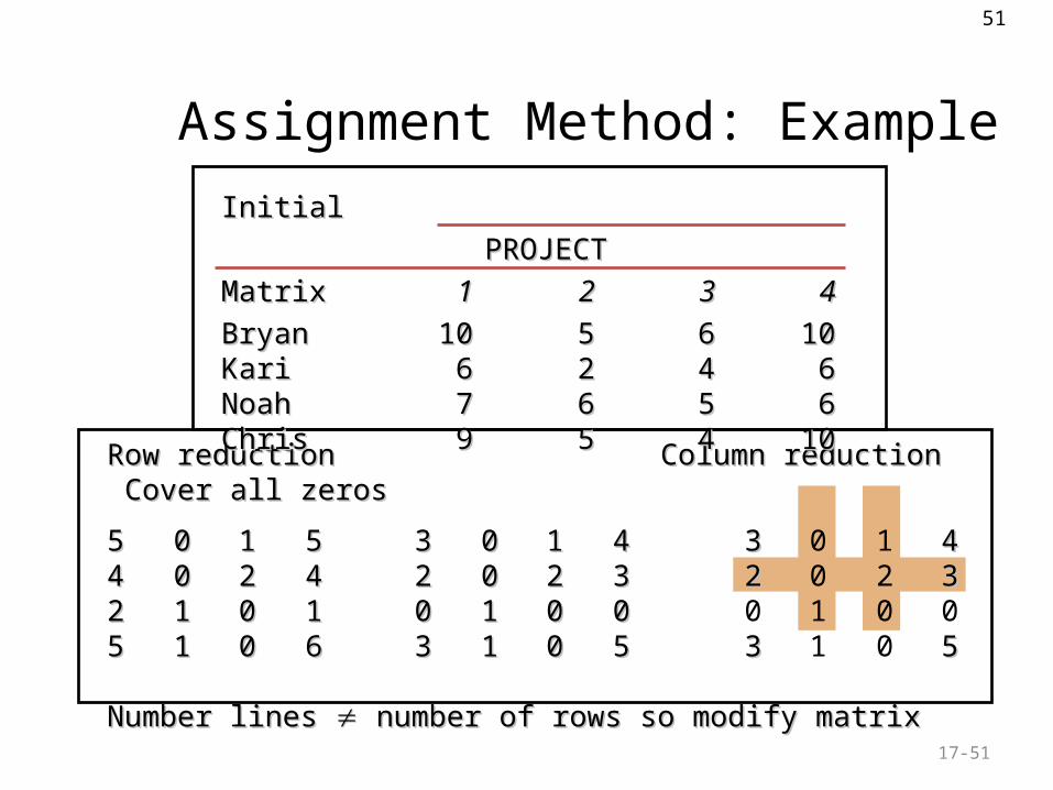
Assignment Method: Example
17-51
Row reductionRow reduction Column reduction Column reduction Cover all zeros Cover all zeros
55 00 11 55 33 00 11 44 33 0 1 4444 00 22 44 22 00 22 33 22 0 2 3322 11 00 11 00 11 00 00 0 1 0 055 11 00 66 33 11 00 55 33 1 0 55
Number lines Number lines number of rows so modify matrix number of rows so modify matrix
Initial PROJECTInitial PROJECT
MatrixMatrix 11 22 33 44
BryanBryan 1010 55 66 1010KariKari 66 22 44 66NoahNoah 77 66 55 66ChrisChris 99 55 44 1010
52
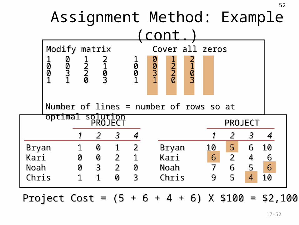
Assignment Method: Example (cont.)
17-52
Modify matrixModify matrix Cover all zerosCover all zeros11 00 11 22 1 0 1 200 00 22 11 0 0 2 100 33 22 00 0 3 2 011 11 00 33 1 1 0 3
Number of lines = number of rows so at optimal solutionNumber of lines = number of rows so at optimal solution
11 22 33 44
BryanBryan 11 00 11 22KariKari 00 00 22 11NoahNoah 00 33 22 00ChrisChris 11 11 00 33
PROJECTPROJECT
11 22 33 44
BryanBryan 1010 5 66 1010KariKari 6 22 44 66NoahNoah 77 66 55 6ChrisChris 99 55 4 1010
PROJECTPROJECT
Project Cost = (5 + 6 + 4 + 6) X $100 = $2,100Project Cost = (5 + 6 + 4 + 6) X $100 = $2,100
53
Sequencing
17-53
Prioritize jobs assigned to a resourceIf no order specified use first-come first-served (FCFS)Other Sequencing Rules
FCFS - first-come, first-servedLCFS - last come, first servedDDATE - earliest due dateCUSTPR - highest customer prioritySETUP - similar required setupsSLACK - smallest slackCR - smallest critical ratioSPT - shortest processing timeLPT - longest processing time

54
Minimum Slack andSmallest Critical Ratio
17-54
CR = =CR = =
If CR > 1, job ahead of scheduleIf CR > 1, job ahead of scheduleIf CR < 1, job behind scheduleIf CR < 1, job behind scheduleIf CR = 1, job on scheduleIf CR = 1, job on schedule
time remainingtime remaining due date - today’s datedue date - today’s date
work remainingwork remaining remaining processing timeremaining processing time
SLACK considers both work and time remainingSLACK considers both work and time remaining
CR recalculates sequence as processing continues and CR recalculates sequence as processing continues and arranges information in ratio formarranges information in ratio form
SLACK = (due date – today’s date) – (processing time)SLACK = (due date – today’s date) – (processing time)
55
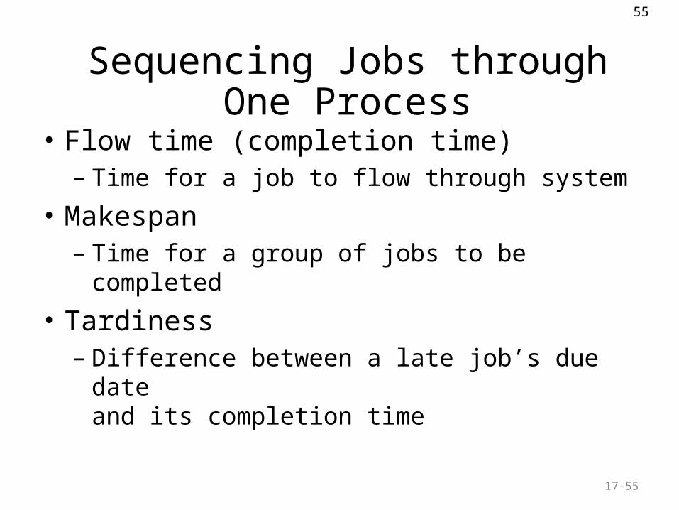
Sequencing Jobs through One Process• Flow time (completion time)
– Time for a job to flow through system
• Makespan– Time for a group of jobs to be completed
• Tardiness– Difference between a late job’s due date
and its completion time
17-55
56
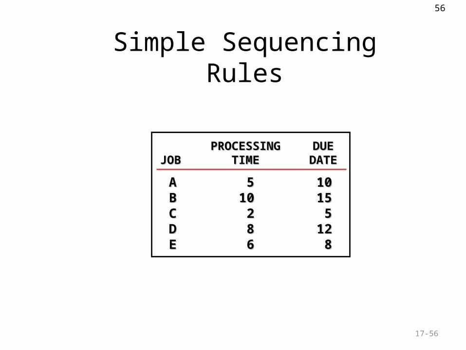
Simple Sequencing Rules
17-56
PROCESSINGPROCESSING DUEDUEJOBJOB TIMETIME DATEDATE
AA 55 1010BB 1010 1515CC 22 55DD 88 1212EE 66 88
57
Simple Sequencing Rules: FCFS
17-57
FCFSFCFS STARTSTART PROCESSINGPROCESSING COMPLETIONCOMPLETION DUEDUESEQUENCESEQUENCE TIMETIME TIMETIME TIMETIME DATEDATE TARDINESSTARDINESS
58
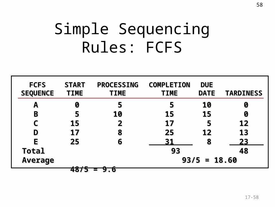
Simple Sequencing Rules: FCFS
17-58
AA 00 55 55 1010 00BB 55 1010 1515 1515 00CC 1515 22 1717 55 1212DD 1717 88 2525 1212 1313EE 2525 66 3131 88 2323
TotalTotal 9393 4848AverageAverage 93/5 = 18.60 93/5 = 18.60 48/5 = 9.6 48/5 = 9.6
FCFSFCFS STARTSTART PROCESSINGPROCESSING COMPLETIONCOMPLETION DUEDUESEQUENCESEQUENCE TIMETIME TIMETIME TIMETIME DATEDATE TARDINESSTARDINESS
59
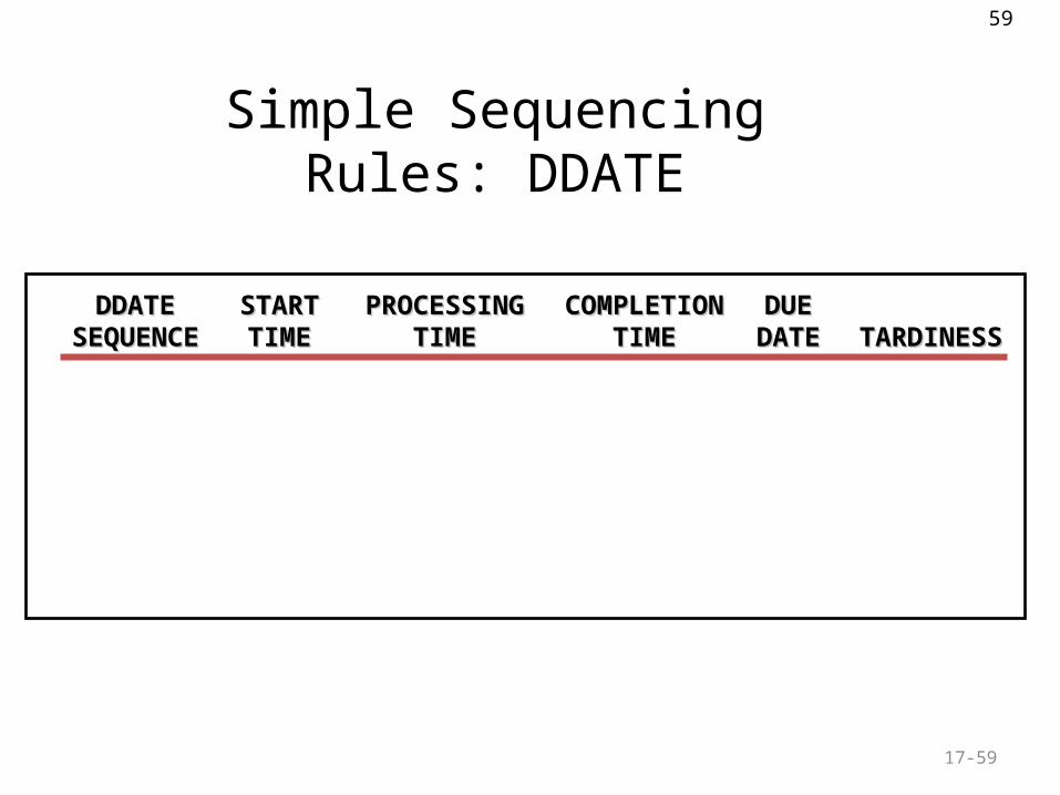
Simple Sequencing Rules: DDATE
17-59
DDATEDDATE STARTSTART PROCESSINGPROCESSING COMPLETIONCOMPLETION DUEDUESEQUENCESEQUENCE TIMETIME TIMETIME TIMETIME DATEDATE TARDINESSTARDINESS

60
Simple Sequencing Rules: DDATE
17-60
CC 00 22 22 55 00EE 22 66 88 88 00AA 88 55 1313 1010 33DD 1313 88 2121 1212 99BB 2121 1010 3131 1515 1616
TotalTotal 7575 2828AverageAverage 75/5 = 15.00 75/5 = 15.00 28/5 = 5.628/5 = 5.6
DDATEDDATE STARTSTART PROCESSINGPROCESSING COMPLETIONCOMPLETION DUEDUESEQUENCESEQUENCE TIMETIME TIMETIME TIMETIME DATEDATE TARDINESSTARDINESS
61
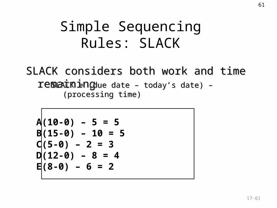
Simple Sequencing Rules: SLACK
17-61
A(10-0) – 5 = 5B(15-0) – 10 = 5C(5-0) – 2 = 3D(12-0) – 8 = 4E(8-0) – 6 = 2
SLACK considers both work and time remainingSLACK considers both work and time remainingSLACK = (due date – today’s date) – (processing time)SLACK = (due date – today’s date) – (processing time)
62
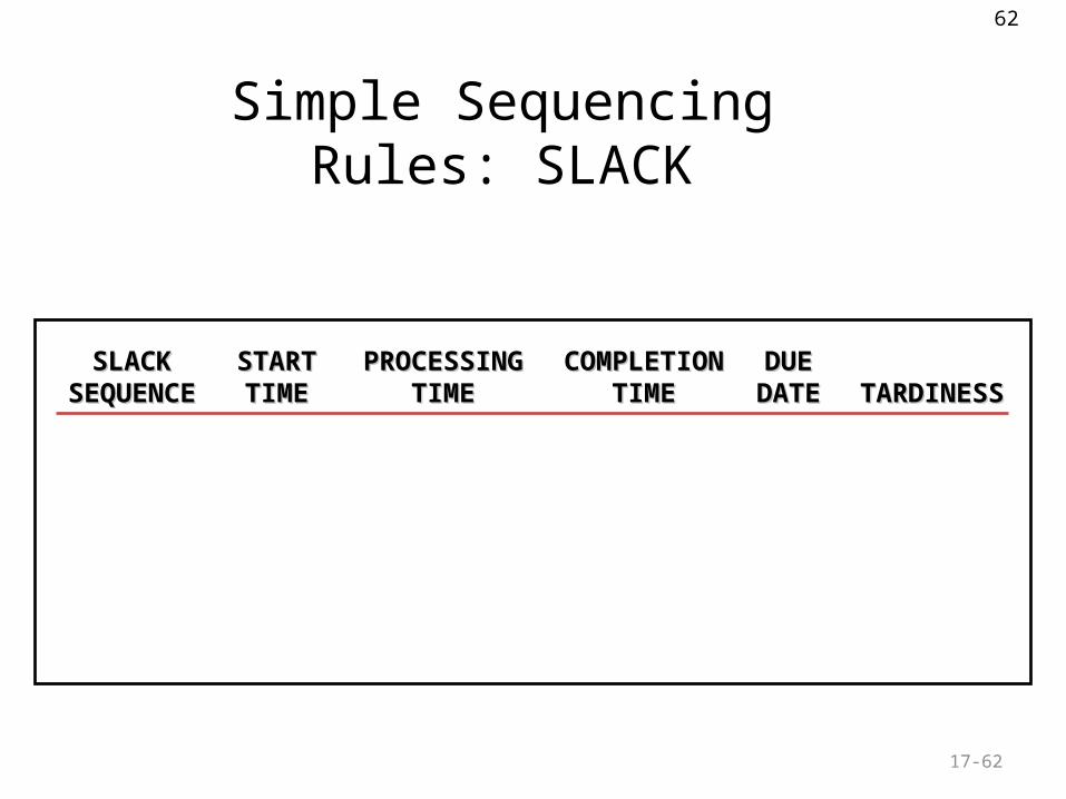
Simple Sequencing Rules: SLACK
17-62
SLACKSLACK STARTSTART PROCESSINGPROCESSING COMPLETIONCOMPLETION DUEDUESEQUENCESEQUENCE TIMETIME TIMETIME TIMETIME DATEDATE TARDINESSTARDINESS
63
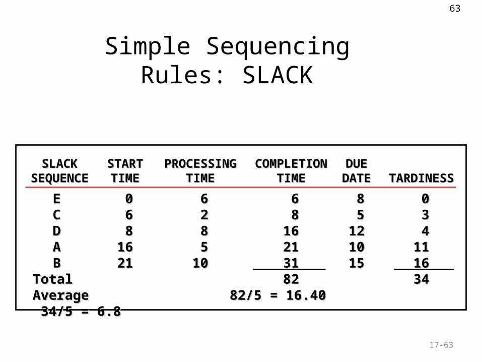
Simple Sequencing Rules: SLACK
17-63
EE 00 66 66 88 00CC 66 22 88 55 33DD 88 88 1616 1212 44AA 1616 55 2121 1010 1111BB 2121 1010 3131 1515 1616
TotalTotal 8282 3434AverageAverage 82/5 = 16.40 34/5 = 6.882/5 = 16.40 34/5 = 6.8
SLACKSLACK STARTSTART PROCESSINGPROCESSING COMPLETIONCOMPLETION DUEDUESEQUENCESEQUENCE TIMETIME TIMETIME TIMETIME DATEDATE TARDINESSTARDINESS
64
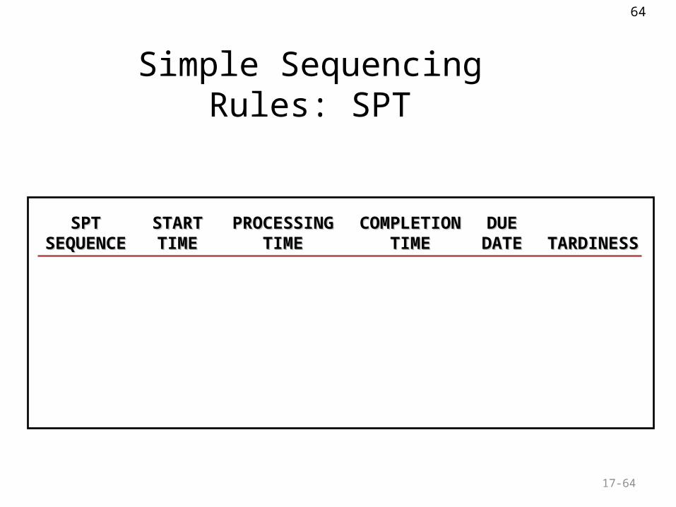
Simple Sequencing Rules: SPT
17-64
SPTSPT STARTSTART PROCESSINGPROCESSING COMPLETIONCOMPLETION DUEDUESEQUENCESEQUENCE TIMETIME TIMETIME TIMETIME DATEDATE TARDINESSTARDINESS
65
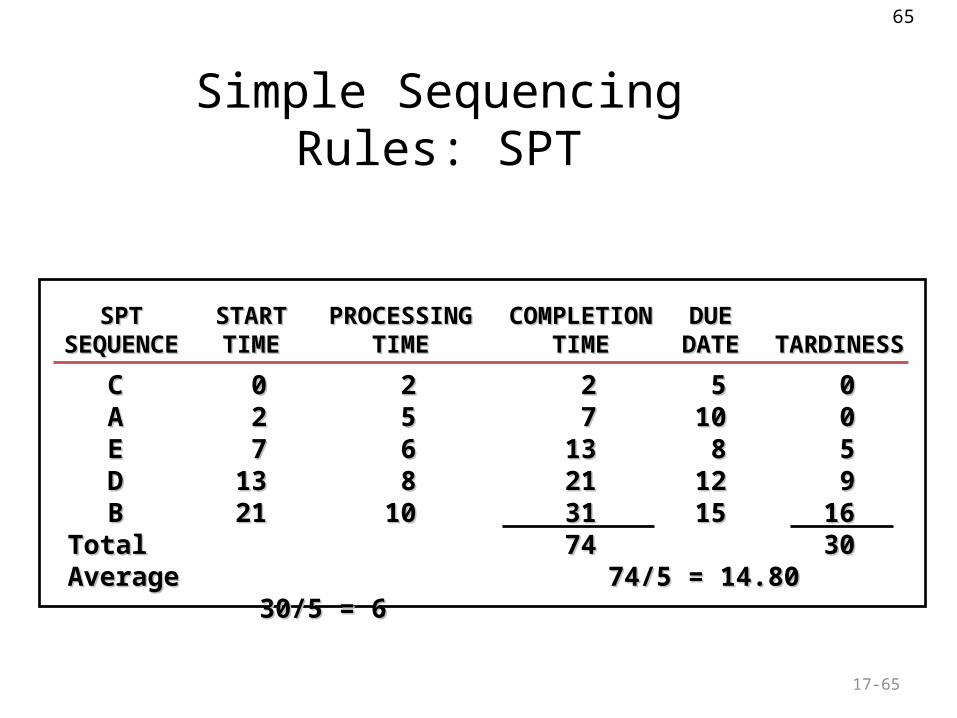
Simple Sequencing Rules: SPT
17-65
CC 00 22 22 55 00AA 22 55 77 1010 00EE 77 66 1313 88 55DD 1313 88 2121 1212 99BB 2121 1010 3131 1515 1616
TotalTotal 7474 3030AverageAverage 74/5 = 14.80 74/5 = 14.80 30/5 = 6 30/5 = 6
SPTSPT STARTSTART PROCESSINGPROCESSING COMPLETIONCOMPLETION DUEDUESEQUENCESEQUENCE TIMETIME TIMETIME TIMETIME DATEDATE TARDINESSTARDINESS
66
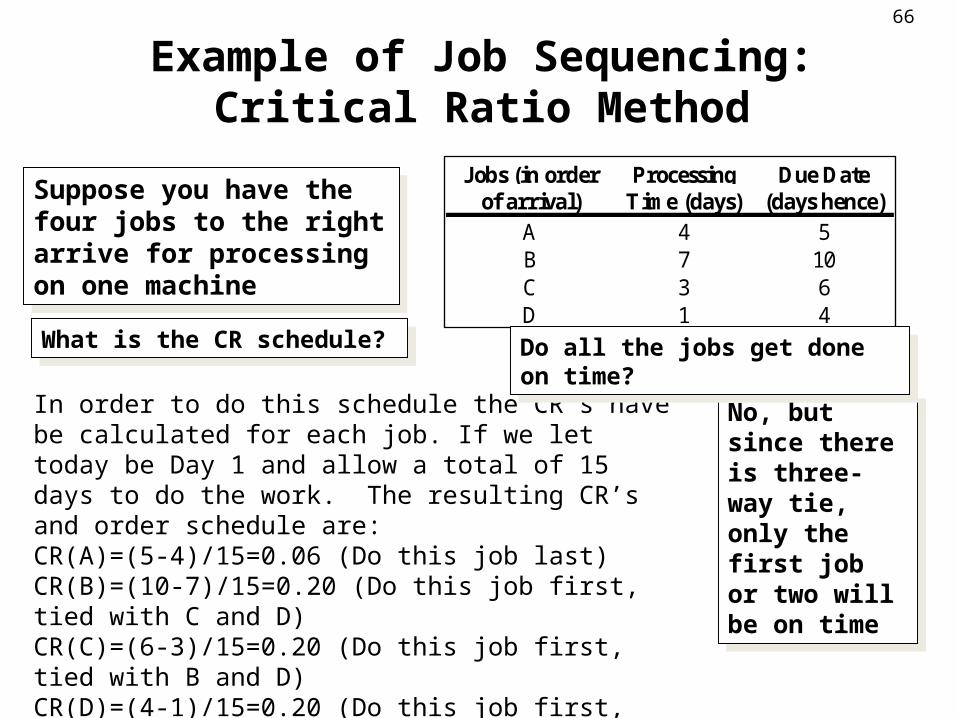
Example of Job Sequencing: Critical Ratio MethodJobs (in order Processing Due Date
of arrival) Time (days) (days hence)A 4 5B 7 10C 3 6D 1 4
Suppose you have the four jobs to the right arrive for processing on one machine
Suppose you have the four jobs to the right arrive for processing on one machine
What is the CR schedule?What is the CR schedule?
No, but since there is three-way tie, only the first job or two will be on time
No, but since there is three-way tie, only the first job or two will be on time
In order to do this schedule the CR’s have be calculated for each job. If we let today be Day 1 and allow a total of 15 days to do the work. The resulting CR’s and order schedule are:CR(A)=(5-4)/15=0.06 (Do this job last)CR(B)=(10-7)/15=0.20 (Do this job first, tied with C and D)CR(C)=(6-3)/15=0.20 (Do this job first, tied with B and D)CR(D)=(4-1)/15=0.20 (Do this job first, tied with B and C)
Do all the jobs get done on time?Do all the jobs get done on time?
67
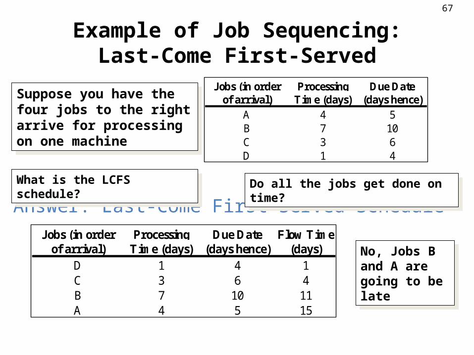
Example of Job Sequencing:Last-Come First-Served
Jobs (in order Processing Due Dateof arrival) Time (days) (days hence)
A 4 5B 7 10C 3 6D 1 4
Answer: Last-Come First-Served ScheduleJobs (in order Processing Due Date Flow Time
of arrival) Time (days) (days hence) (days)D 1 4 1C 3 6 4B 7 10 11A 4 5 15
No, Jobs B and A are going to be late
No, Jobs B and A are going to be late
Suppose you have the four jobs to the right arrive for processing on one machine
Suppose you have the four jobs to the right arrive for processing on one machine
What is the LCFS schedule?What is the LCFS schedule?Do all the jobs get done on time?Do all the jobs get done on time?
68
Simple Sequencing Rules: Summary
17-68
AVERAGEAVERAGE AVERAGEAVERAGE NO. OFNO. OF MAXIMUMMAXIMUMRULERULE COMPLETION TIMECOMPLETION TIME TARDINESSTARDINESS JOBS TARDYJOBS TARDY TARDINESSTARDINESS
69
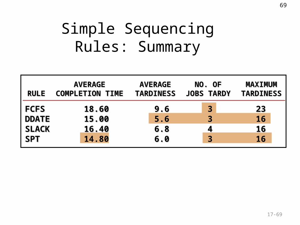
Simple Sequencing Rules: Summary
17-69
FCFSFCFS 18.6018.60 9.69.6 3 2323DDATEDDATE 15.0015.00 5.6 3 16SLACKSLACK 16.4016.40 6.86.8 44 1616SPTSPT 14.80 6.06.0 3 16
AVERAGEAVERAGE AVERAGEAVERAGE NO. OFNO. OF MAXIMUMMAXIMUMRULERULE COMPLETION TIMECOMPLETION TIME TARDINESSTARDINESS JOBS TARDYJOBS TARDY TARDINESSTARDINESS
70
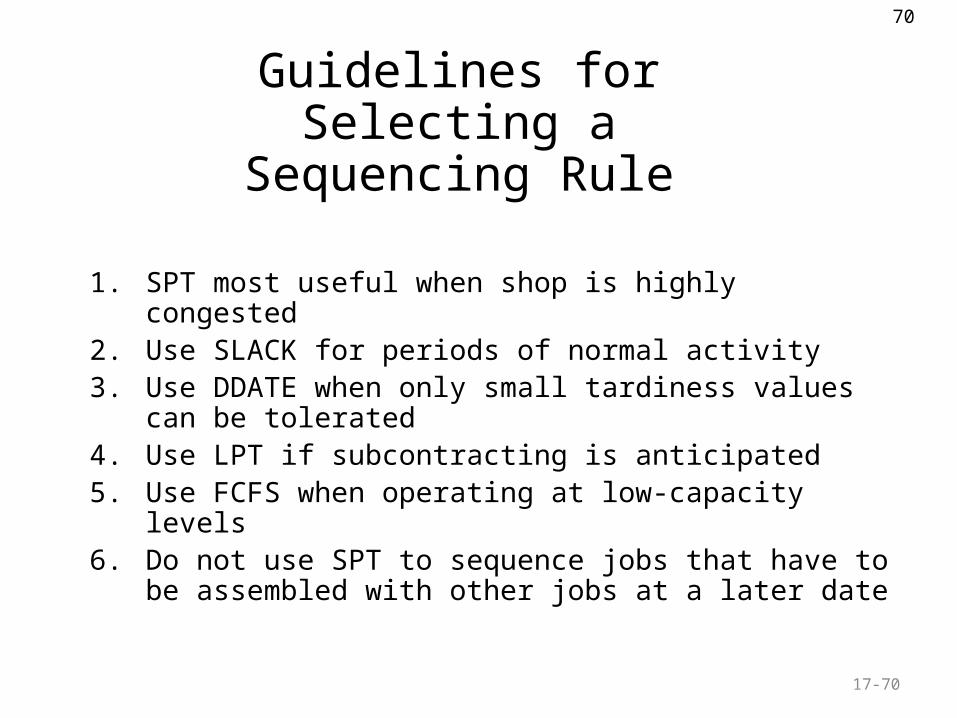
Guidelines for Selecting a Sequencing Rule
1. SPT most useful when shop is highly congested2. Use SLACK for periods of normal activity3. Use DDATE when only small tardiness values can be
tolerated4. Use LPT if subcontracting is anticipated5. Use FCFS when operating at low-capacity levels6. Do not use SPT to sequence jobs that have to be
assembled with other jobs at a later date
17-70
71
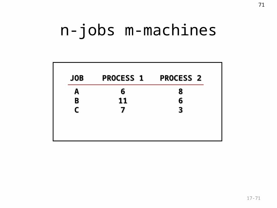
n-jobs m-machines
17-71
JOBJOB PROCESS 1PROCESS 1 PROCESS 2PROCESS 2
AA 66 88BB 1111 66CC 77 33
72
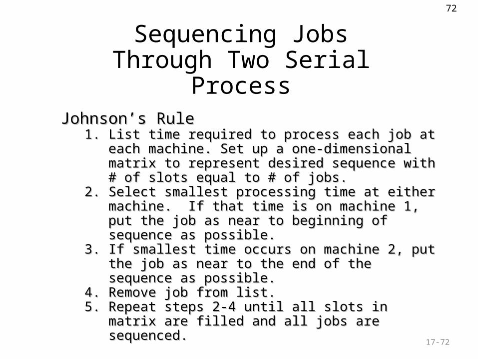
Sequencing Jobs Through Two Serial Process
17-72
Johnson’s RuleJohnson’s Rule1.1. List time required to process each job at each machine. Set List time required to process each job at each machine. Set
up a one-dimensional matrix to represent desired sequence up a one-dimensional matrix to represent desired sequence with # of slots equal to # of jobs.with # of slots equal to # of jobs.
2.2. Select smallest processing time at either machine. If that Select smallest processing time at either machine. If that time is on machine 1, put the job as near to beginning of time is on machine 1, put the job as near to beginning of sequence as possible.sequence as possible.
3.3. If smallest time occurs on machine 2, put the job as near to If smallest time occurs on machine 2, put the job as near to the end of the sequence as possible.the end of the sequence as possible.
4.4. Remove job from list.Remove job from list.5.5. Repeat steps 2-4 until all slots in matrix are filled and all jobs Repeat steps 2-4 until all slots in matrix are filled and all jobs
are sequenced.are sequenced.
73
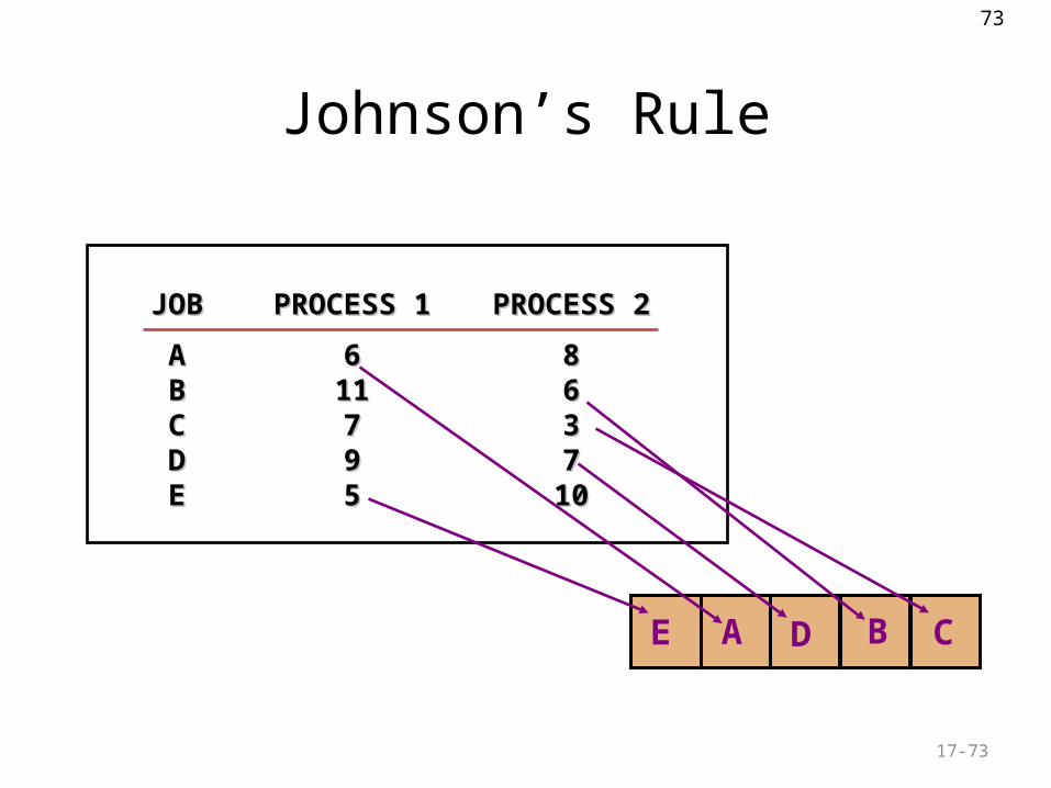
Johnson’s Rule
17-73
JOBJOB PROCESS 1PROCESS 1 PROCESS 2PROCESS 2
AA 66 88BB 1111 66CC 77 33DD 99 77EE 55 1010
CE A BD
74
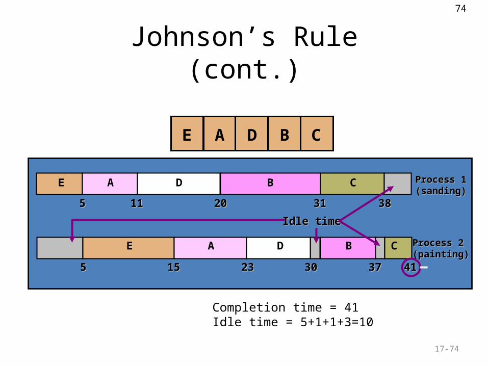
Johnson’s Rule (cont.)
17-74
A B CDE
E A D B C Process 1Process 1(sanding)(sanding)
55 1111 2020 3131 3838
E A D B C Process 2Process 2(painting)(painting)
55 1515 2323 3030 3737 4141
Idle timeIdle time
Completion time = 41Idle time = 5+1+1+3=10
75
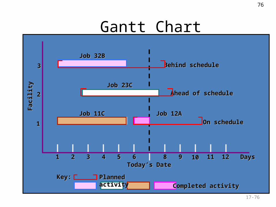
Monitoring
• Work package– Shop paperwork that travels with a job
• Gantt Chart– Shows both planned and completed activities
against a time scale• Input/Output Control
– Monitors the input and output from each work center
17-75
76
Gantt Chart
17-76
11 22 33 44 55 66 88 99 1010 1111 1212 DaysDays
11
22
33
Today’s DateToday’s Date
Job 32BJob 32B
Job 23CJob 23C
Job 11CJob 11C Job 12AJob 12A
Fac
ilit
yF
acil
ity
Key:Key: Planned activityPlanned activity
Completed activityCompleted activity
Behind scheduleBehind schedule
Ahead of scheduleAhead of schedule
On scheduleOn schedule
77
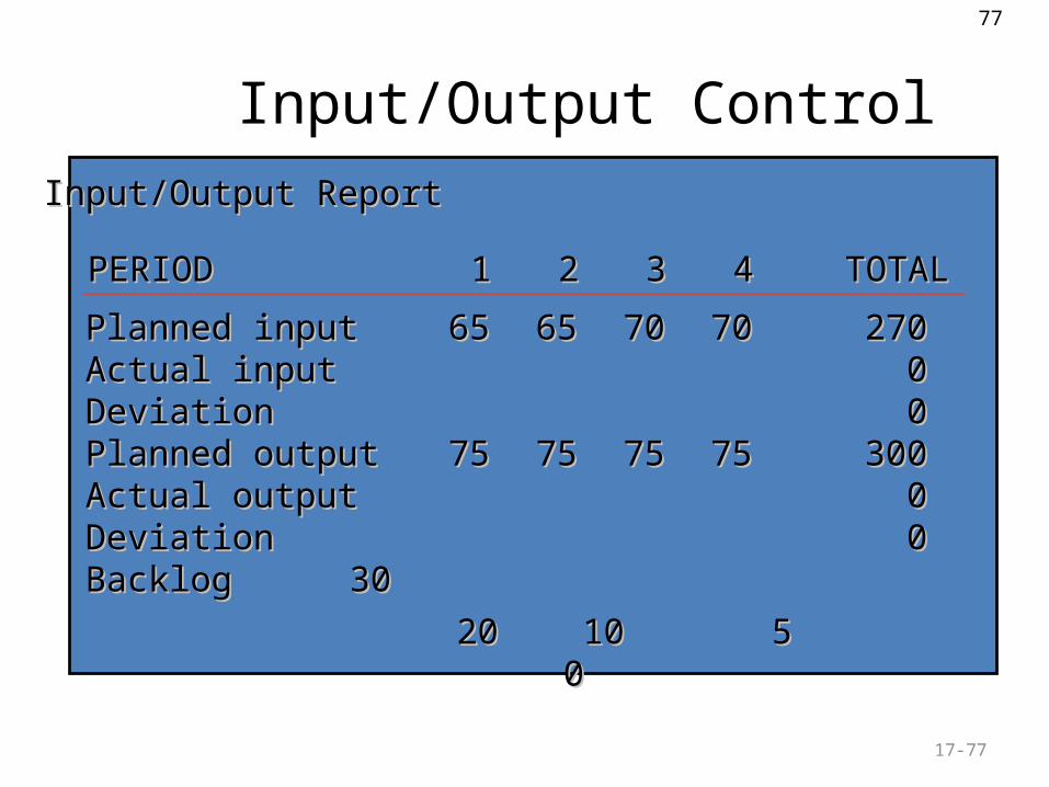
Input/Output Control
17-77
Input/Output ReportInput/Output Report
Planned inputPlanned input 6565 6565 7070 7070 270270Actual inputActual input 00DeviationDeviation 00Planned outputPlanned output 7575 7575 7575 7575 300300Actual outputActual output 00DeviationDeviation 00BacklogBacklog 3030
PERIODPERIOD 11 22 33 44 TOTALTOTAL
20 10 5 020 10 5 0
78
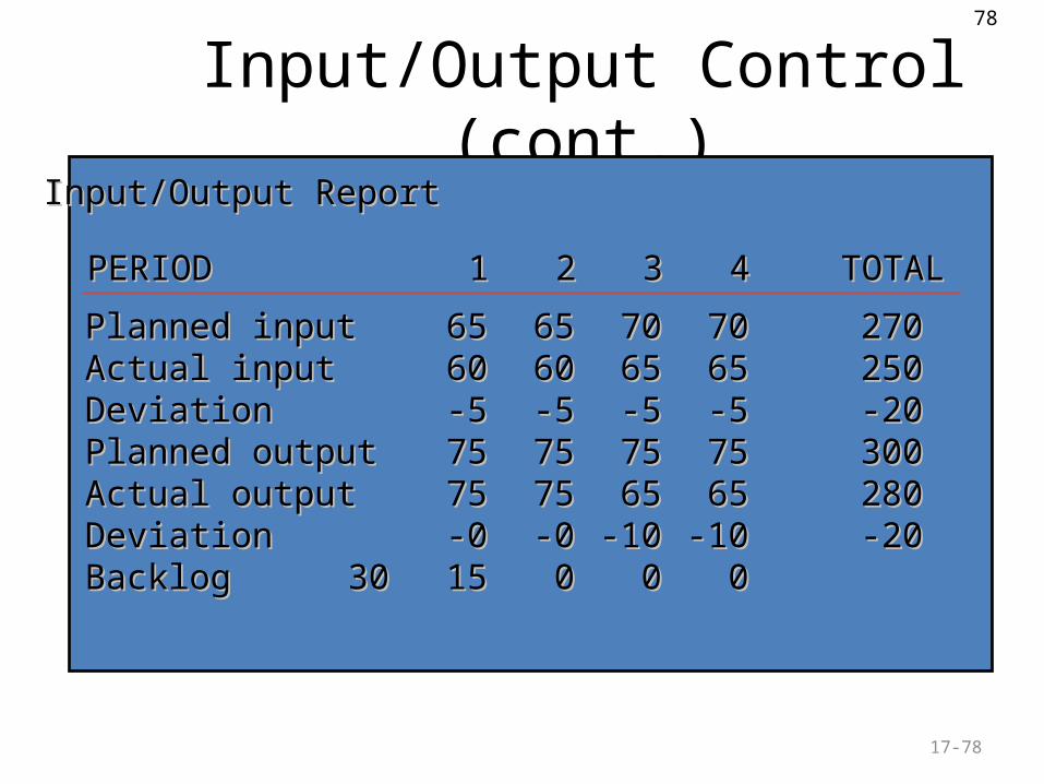
Input/Output Control (cont.)
17-78
Input/Output ReportInput/Output Report
Planned inputPlanned input 6565 6565 7070 7070 270270Actual inputActual input 6060 6060 6565 6565 250250DeviationDeviation -5-5 -5-5 -5-5 -5-5 -20-20Planned outputPlanned output 7575 7575 7575 7575 300300Actual outputActual output 7575 7575 6565 6565 280280DeviationDeviation -0-0 -0-0 -10-10 -10-10 -20-20BacklogBacklog 3030 1515 00 00 00
PERIODPERIOD 11 22 33 44 TOTALTOTAL
79
Supply Chain Management:
80
Some Definitions
Supply Chain Management encompasses every effort involved in producing and delivering a final product or service, from the supplier’s supplier to the customer’s customer. Supply Chain Management includes managing supply and demand, sourcing raw materials and parts, manufacturing and assembly, warehousing and inventory tracking, order entry and order management, distribution across all channels, and delivery to the customer.
The Supply Chain Council, U.S.A.
81
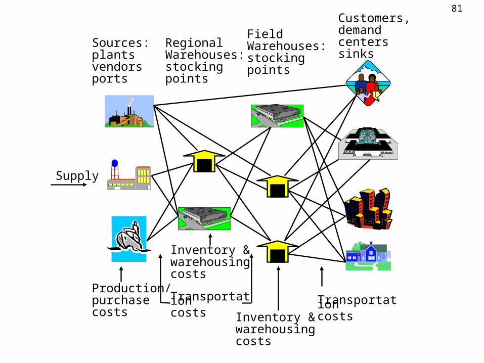
Supply
Sources:plantsvendorsports
RegionalWarehouses:stocking points
Field Warehouses:stockingpoints
Customers,demandcenterssinks
Production/purchase costs
Inventory &warehousing costs
Transportation costs Inventory &
warehousing costs
Transportation costs
82
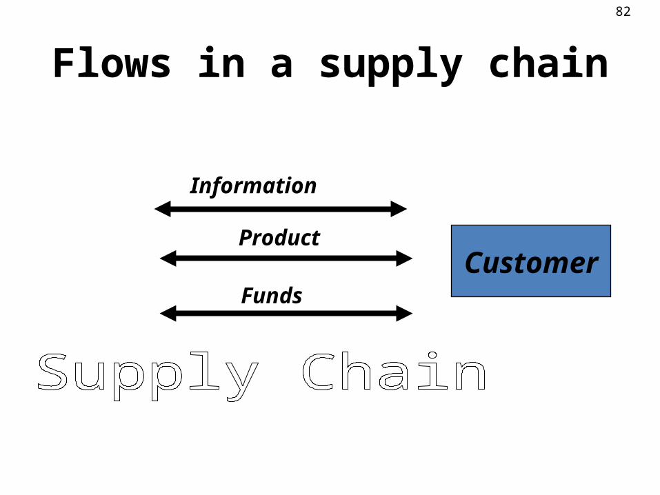
Flows in a supply chain
Customer
Information
Product
Funds
83
Philosophy of SCM
• The entire supply chain is a single, integrated entity.
• The cost, quality and delivery requirements of the customer are objectives shared by every company in the chain.
• Inventory is the last resort for resolving supply and demand imbalances.
84
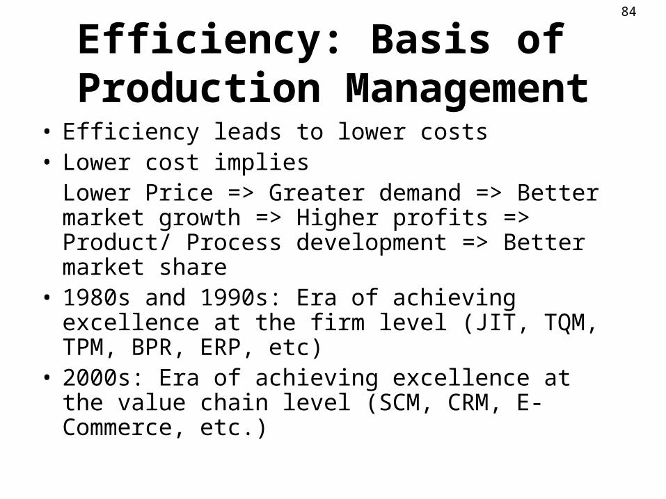
Efficiency: Basis of Production Management
• Efficiency leads to lower costs• Lower cost implies
Lower Price => Greater demand => Better market growth => Higher profits => Product/ Process development => Better market share
• 1980s and 1990s: Era of achieving excellence at the firm level (JIT, TQM, TPM, BPR, ERP, etc)
• 2000s: Era of achieving excellence at the value chain level (SCM, CRM, E-Commerce, etc.)
85
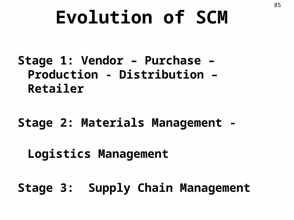
Evolution of SCM
Stage 1: Vendor – Purchase – Production - Distribution – Retailer
Stage 2: Materials Management -
Logistics Management
Stage 3: Supply Chain Management
86
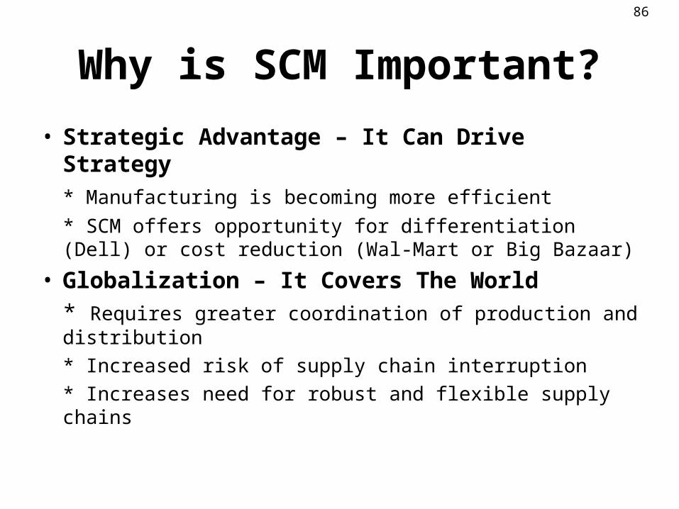
Why is SCM Important?
• Strategic Advantage – It Can Drive Strategy* Manufacturing is becoming more efficient* SCM offers opportunity for differentiation (Dell) or cost reduction (Wal-Mart or Big Bazaar)
• Globalization – It Covers The World* Requires greater coordination of production and distribution* Increased risk of supply chain interruption* Increases need for robust and flexible supply chains

87
Why is SCM Important?(continued)
• At the company level, supply chain management impacts* COST – For many products, 20% to 40% of total product costs are controllable logistics costs. * SERVICE – For many products, performance
factors such as inventory availability and speed of delivery are critical to customer satisfaction.
88
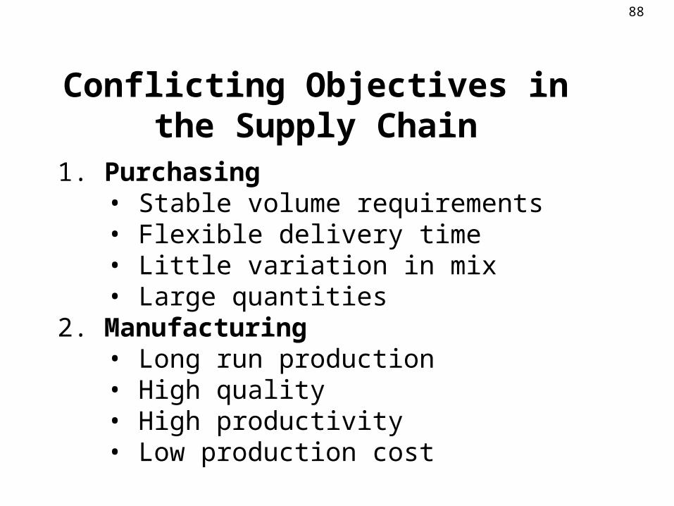
Conflicting Objectives in the Supply Chain
1. Purchasing• Stable volume requirements • Flexible delivery time• Little variation in mix• Large quantities
2. Manufacturing• Long run production• High quality• High productivity• Low production cost
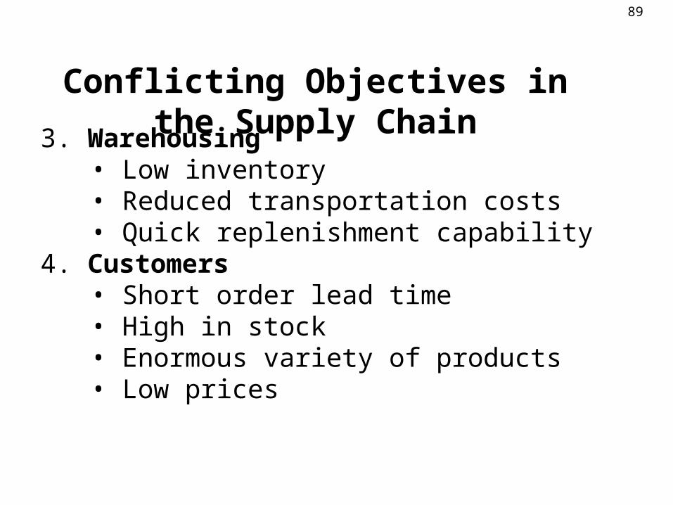
89
Conflicting Objectives in the Supply Chain3. Warehousing
• Low inventory • Reduced transportation costs• Quick replenishment capability
4. Customers• Short order lead time• High in stock• Enormous variety of products• Low prices
90
Decision Phases in a Supply Chain
• Supply chain strategy or design• Supply chain planning• Supply chain operation
91
Process view of a supply chain
• Cycle view
• Push/pull view
92
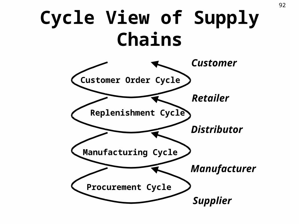
Cycle View of Supply Chains
Customer Order Cycle
Replenishment Cycle
Manufacturing Cycle
Procurement Cycle
Customer
Retailer
Distributor
Manufacturer
Supplier
93
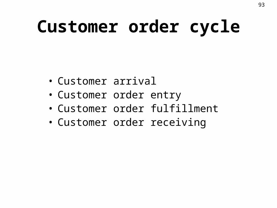
Customer order cycle
• Customer arrival• Customer order entry• Customer order fulfillment• Customer order receiving
94
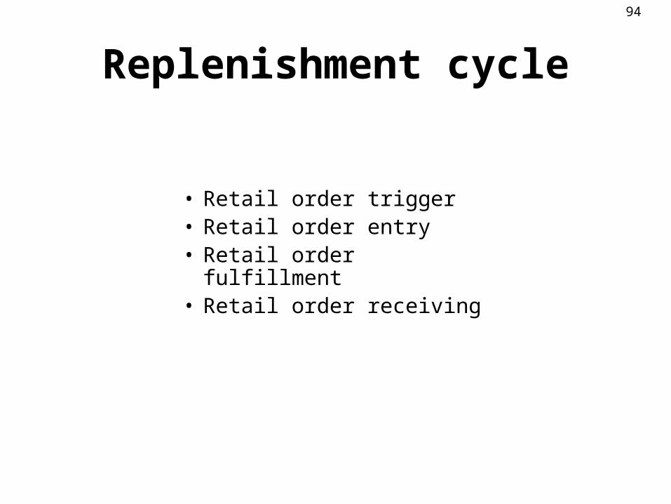
Replenishment cycle
• Retail order trigger• Retail order entry• Retail order fulfillment• Retail order receiving

95
Manufacturing cycle
• Order arrival from the distributor, retailer, or customer
• Production scheduling• Manufacturing and shipping• Receiving at the distributor, retailer, or
customer
96
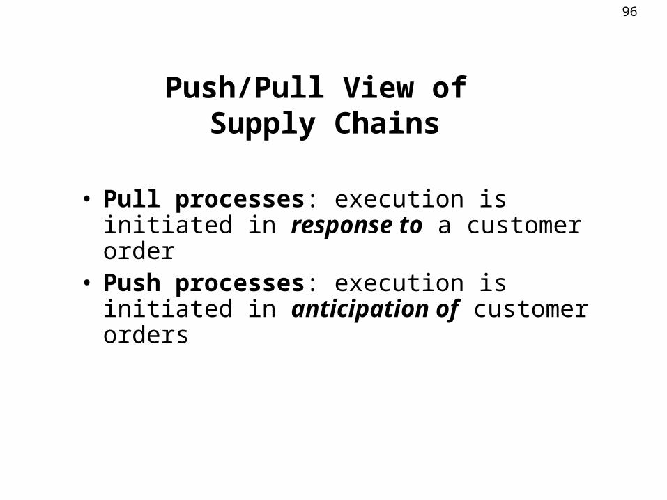
Push/Pull View of Supply Chains
• Pull processes: execution is initiated in response to a customer order
• Push processes: execution is initiated in anticipation of customer orders
97
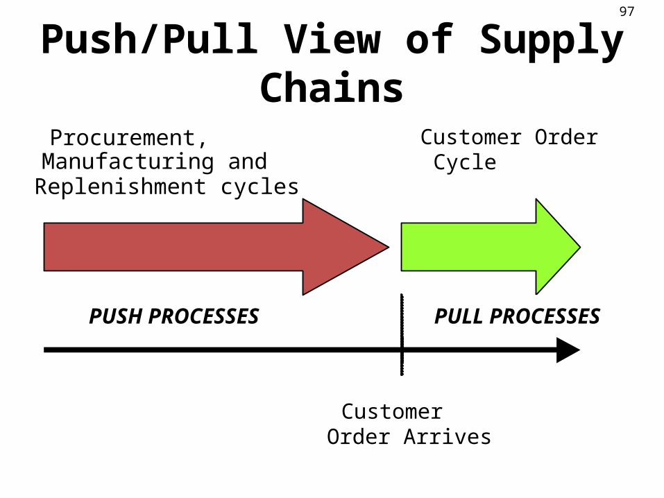
Push/Pull View of Supply Chains
Procurement,Manufacturing andReplenishment cycles
Customer OrderCycle
CustomerOrder Arrives
PUSH PROCESSES PULL PROCESSES

98SUPPLY CHAIN DESIGN:Three Components
1. Insourcing/OutSourcing(The Make/Buy or Vertical Integration Decision) 2. Partner Selection(Choice of suppliers and partners for the chain) 3. The Contractual Relationship(Arm's length, joint venture, long-term contract,strategic alliance, equity participation, etc.)
99
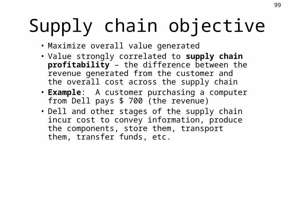
Supply chain objective• Maximize overall value generated• Value strongly correlated to supply chain
profitability – the difference between the revenue generated from the customer and the overall cost across the supply chain
• Example: A customer purchasing a computer from Dell pays $ 700 (the revenue)
• Dell and other stages of the supply chain incur cost to convey information, produce the components, store them, transport them, transfer funds, etc.

100
Examples of Supply Chains
• Dell / Compaq• Toyota / GM / Ford• Milk Distribution System of NDDB• Merry-Go-Round System of NTPC• Dabbawalas of Mumbai• Amazon / Borders / Barnes and Noble
101O
rde
r S
ize
Time
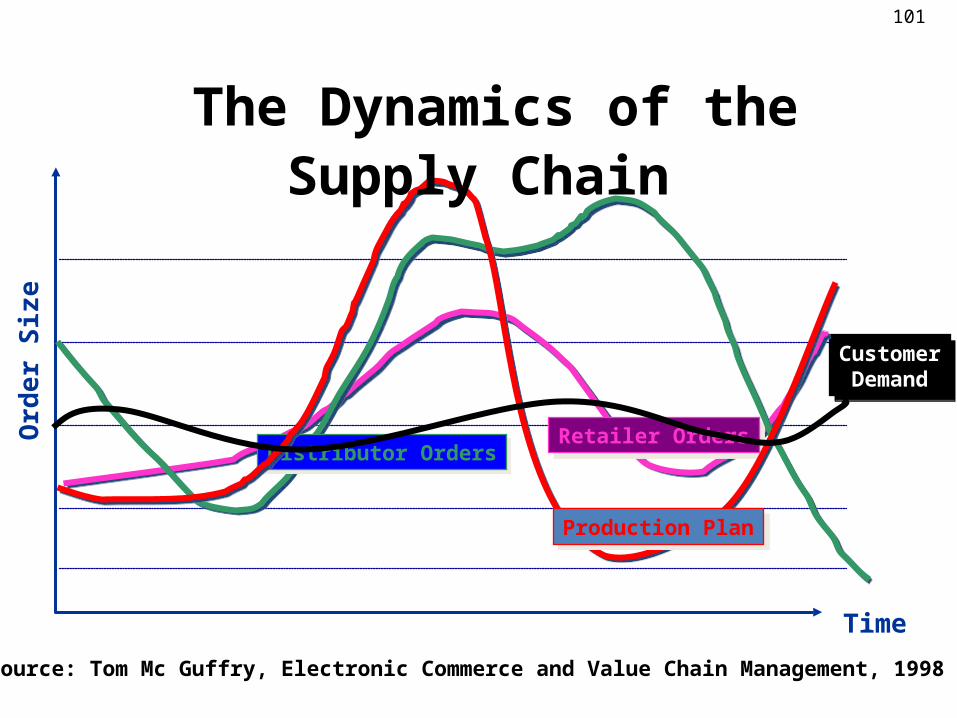
Source: Tom Mc Guffry, Electronic Commerce and Value Chain Management, 1998
CustomerDemand
CustomerDemand
Retailer OrdersRetailer OrdersDistributor OrdersDistributor Orders
Production PlanProduction Plan
The Dynamics of the Supply Chain
102
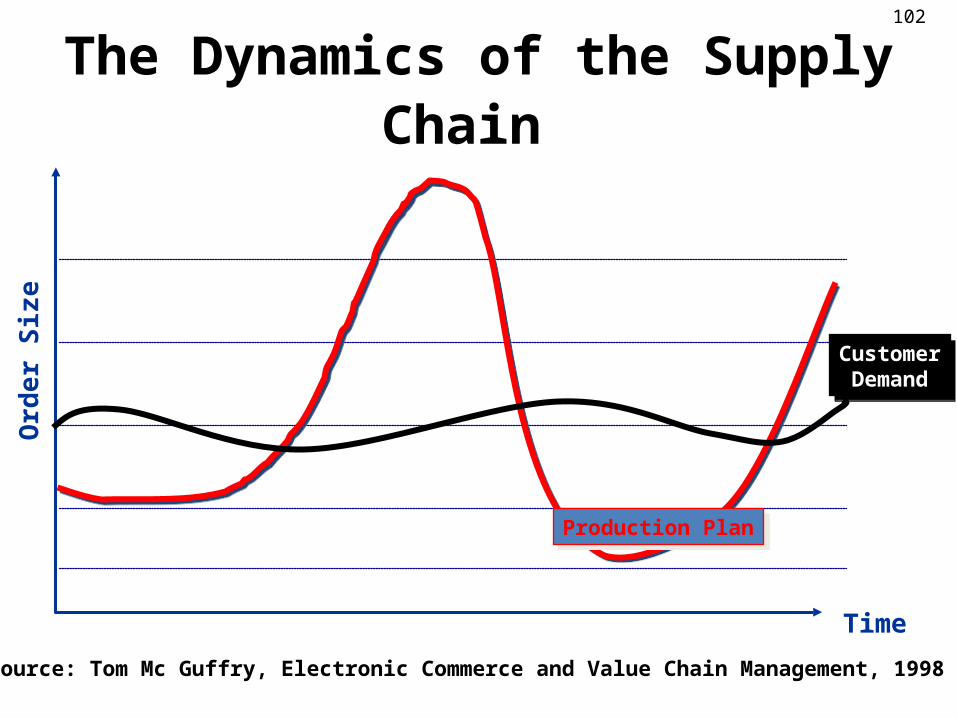
The Dynamics of the Supply Chain O
rde
r S
ize
Time
Source: Tom Mc Guffry, Electronic Commerce and Value Chain Management, 1998
CustomerDemand
CustomerDemand
Production PlanProduction Plan