integrating planning & scheduling subbarao kambhampati integrating planning & scheduling...

Integrating Planning & Scheduling Subbarao Kambhampati

Integrating Planning & Scheduling

Agenda:

Questions on Scheduling?

Discussion on Smith’s paper?

Next topic: Nondeterministic Planning


Dana Nau’s visit..

Talk on 3/31 afternoon (Monday)– Planning for Interactions among Autonomous Agents

May come to the class on 4/1 (Tuesday)– Can pick his brains…


Temporal Planning & Scheduling

What we did: Action representations Search models

– Completeness considerations

Temporal networks Scheduling

Some outstanding issues Integrating planning &

scheduling Heuristics for temporal

planning


Need for Integration Most existing planners

concentrate on action selection, ignoring resource allocation– Plan-based interfaces– Interactive decision support

Most existing schedulers concentrate only on resource allocation, ignoring action selection– E.g. HSTS operation

scheduling

Many real-world problems require both capabilities– Supply Chain Management problems

» I2, ILOG, Manugistics

– Planning in domains with durative actions, continuous change

» NASA RAX experiment


Why now?

Significant scale-up in plan synthesis in last 4-5 years– 5/6 action plans in minutes to 100 action plans in

minutes – Breakthroughs in search space representation, heuristic

and domain-specific

Significant strides in our understanding of connections between planning and scheduling– Rich connections between planning and CSP/SAT/ILP

» Vanishing separation between planning techniques and scheduling techniques


Approaches for Integration

Extend schedulers to handle action and resource choices

Extend planners to deal with resources, durative actions and continuous quantities

Coupled Architectures– De-coupled– Loosely Coupled (RealPlan System)

PLAN

NER

SCH

EDULE

RCausal Pla

n

Schdule

job-shopscheduling

planning

resourcechoices(RCSP)

alternativeprocesses

process3 process7process8

Task1

Task2

Task3

Task4

Task5

Task6

Task8

Task7

…

…… … …

… …


Approaches

Decoupled– Existing approaches

Monolithic– Extend Planners to handle time and resources– Extend Schedulers to handle choice

Loosely Coupled– Making planners and schedulers interact


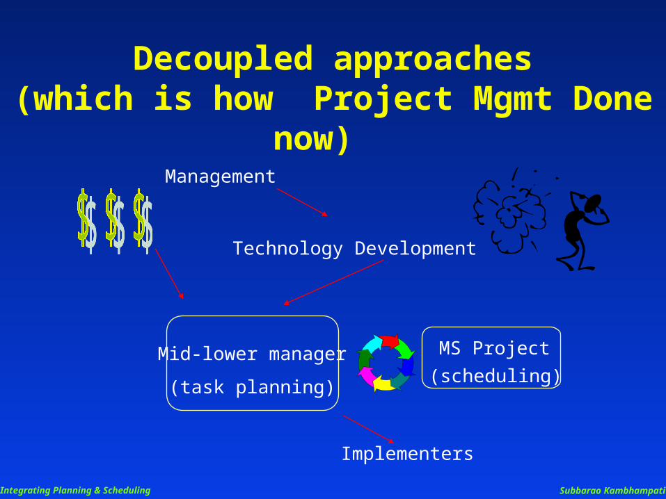
Decoupled approaches(which is how Project Mgmt Done now)

Management

Technology Development

Mid-lower manager

Implementers

MS Project

(task planning)(scheduling)


Extending Planners

ZENO [Penberthy & Weld], IxTET [Ghallab & Laborie], HSTS/RAX [Muscettola] extend a conjunctive plan-space planner with temporal and numeric constraint reasoners

LPSAT [Wolfman & Weld] integrates a disjunctive state-space planner with an LP solver to support numeric quantities

IPPlan [Kautz & Walser; 99] constructs ILP encodings with numeric constraints

TGP [Smith & Weld; 99] supports actions with durations in Graphplan

HSTSPlan Database

Model(DDL)

Searchengine

Engine

Goals

Initial state

Plan

Domain Knowledge

PlanningExperts

from EXEC

SearchControl

to EXEC


Actions with Resources and Duration

Load(P:package, R:rocket, L:location)

Resources: ?h : robot hand Preconditions: Position(?h,L) [?s, ?e] Free(?h) ?s Charge(?h) > 5 ?s

Effects: holding(?h, P) [?s, ?t1] depositing(?h,P,R) [?t2, ?e] Busy(?h) [?s, ?e] Free(?h) ?e Charge - = .03*(?e - ?s) ?e

Constraints: ?t1 < ?t2 ?e - ?s in [1.0, 2.0]

Capacity(robot) = 3

?s ?e

Pos(?h,L)

Hold(?h,P)dep(?h,P)

[1,2]

Free(?h) Free(?h)Busy(?h)


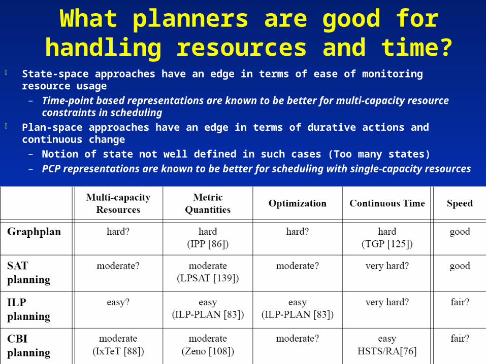
What planners are good for handling resources and time?

State-space approaches have an edge in terms of ease of monitoring resource usage– Time-point based representations are known to be better for multi-capacity

resource constraints in scheduling Plan-space approaches have an edge in terms of durative actions and continuous

change– Notion of state not well defined in such cases (Too many states)– PCP representations are known to be better for scheduling with single-capacity

resources


Smith’s Table


Extending Scheduling

job-shopscheduling

planning

resourcechoices(RCSP)

alternativeprocesses

process3 process7process8

Task1

Task2

Task3

Task4

Task5

Task6

Task8

Task7

Ordering choicesResource choicesProcess choices


Monolithic Architectures Scale Poorly

Extended planning systems are hard to control

– RAX uses a very error-prone hand-coded search control strategy

Extended scheduling systems tend to lose effectiveness due to increased disjunction

Monolithic systems can sometimes show counter-intuitive behavior (by multiplying search failures)

D

C

E

B

F

A

E

B

A

F

D

C

Total

Search

Graph

Performance worsens with increased resources!


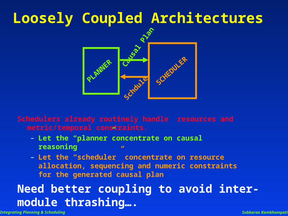
Loosely Coupled Architectures

Schedulers already routinely handle resources and metric/temporal constraints. – Let the “planner”concentrate on causal reasoning– Let the “scheduler” concentrate on resource

allocation, sequencing and numeric constraints for the generated causal plan

PLANNER

SCHEDULE

R

Cau

sal P

lan

Schd

ule

Need better coupling to avoid inter-module thrashing….


Making Loose Coupling Work

How can the Planner keep track of consistency?

– Low level constraint propagation

» Loose path consistency on TCSPs

» Bounds on resource consumption,

» LP relaxations of metric constraints

– Pre-emptive conflict resolution

The more aggressive you do this, the less need for a scheduler.. How do the modules interact?

– Failure explanations; Partial results

PLAN

NER

SCH

EDULE

RCausal Pla

n

Schdule


RealPlan--Master/Slave

PS

Master-Slave(RealPlan-MS)

Variables: ActionsValues: Resources

Planner does causal reasoning.

Scheduler attempts resource allocation If scheduler fails, planner has to restart

[Sriv

astava

&

Kam

bhampati

ECP,9

9;

AAAI,

2000]

Planner’s CSP: Variables: “goals” Values: “actions”

Scheduler’s CSP: Variables: “Actions” Values: “Resources”

Resou

rce c

onstr

aint

s

activ

ated

by

the

sele

cted

acto

ns


Performance of Master-Slave Coupling

When sc

heduler f

ails, n

o

specifi

c guid

ance is

given

to th

e planner


RealPlan: Peer-to-Peer

SP T

Peer-Peer (RealPlan-PP)

Variables: FactsValues: Actions

Variables: ActionsValues: Resources

Explanation-dire

cted

backtracking b

etween

Planner and Scheduler

Planner’s CSP: Variables: “goals” Values: “actions”

Scheduler’s CSP: Variables: “Actions” Values: “Resources”

Set o

f act

ions

that

cann

ot b

e sch

edul

ed

Resou

rce c

onstr

aint

s

activ

ated

by

the

sele

cted

acto

ns


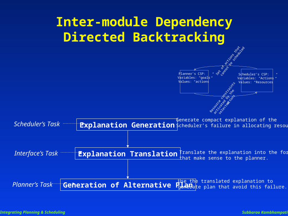
Inter-module Dependency Directed Backtracking

Explanation Generation

Explanation Translation

Generation of Alternative Plan

Scheduler’s Task

Interface’s Task

Planner’s Task

Generate compact explanation of theScheduler’s failure in allocating resources

Translate the explanation into the formthat make sense to the planner.

Use the translated explanation togenerate plan that avoid this failure.

Planner’s CSP:Variables: “goals”Values: “actions”

Scheduler’s CSP:Variables: “Actions”Values: “Resources”

Set o

f act

ions

that

cann

ot b

e sch

edul

ed

Resou

rce c

onstr

aint

s

activ

ated

by

the

sele

cted

act

ons


Resource Domains:A1, A2 , A3: {R1 , R2}A4, A5: {S1 , S2 , S3}

Resource Constraints:A1 A2 ; A2 A3 ;A1 A3 ; A4 A5 ;

N1: {A1 = R1}

N1: {A1 = R1, A2 = R2}

N1: {A1 = R1, A2 = R2 , A4 = S1}

N1: {A1 = R1, A2 = R2 , A4 = S1 , A3 = R1} N1: {A1 = R1, A2 = R2 , A4 = S1 , A3 = R2}

A1 = R1

A2 = R2

A4 = S1

A3 = R1 A3 = R2

Subset of variables that can not beassigned values (reason of failure):

(A1 , A2 , A3)


Shuffle 8 Blocks

1

10

100

1000

10000

100000

2 3 4 5

Robot hand

Tim

e (s

ec)

Realplan-PPRealplan-MS

RealPlan-PP RealPlan-MS Speedup (x)ProblemClass Time #bk

BTPWFTime Class Time BTPWF RealP

lan-MS

Shuf_b8r4

Shuf_b8r4

INFRES

FIX

2.52

8.74

4

1

>3 hr

>3 hr

SAMELEN

SAMELEN

9373

9373

>4170

>1236

3619

1072

Huge_r6 INFRES 4.53 4 976 INCRLEN 11056 215 2441

Huge_r6

Huge_r6

FIX

SAMELEN

17.48

20.59

3

2

991

983

INCRLEN

INCRLEN

11056

11056

56.7

47.7

632

537


A temporal plannersupporting causal plan synthesis

CSP-basedFinite capacityresource scheduler

Mixed Integer/Linearprogramming modulefor metric constraints

Mission Profile

Executor

inte

rfac

e

interface

interface

Plans with annotatedwaypoints

Execution statusReplanning requests

Mission modificationsPlan criticism

Evolving specs

Next-Generation Realplan


Summary & Conclusion

Motivated the need for integrating Planning and Scheduling

Discussed the state of the art in Planning and Scheduling

Discussed approaches for Integrating them– Loosely coupled architectures are a promising

approach

26

Multi-objective search

Multi-dimensional nature of plan quality in metric temporal planning: Temporal quality (e.g. makespan, slack—the time when a

goal is needed – time when it is achieved.) Plan cost (e.g. cumulative action cost, resource consumption)

Necessitates multi-objective optimization: Modeling objective functions Tracking different quality metrics and heuristic estimation Challenge: There may be inter-dependent

relations between different quality metric

27

Example

Option 1: Tempe Phoenix (Bus) Los Angeles (Airplane) Less time: 3 hours; More expensive: $200

Option 2: Tempe Los Angeles (Car) More time: 12 hours; Less expensive: $50

Given a deadline constraint (6 hours) Only option 1 is viable Given a money constraint ($100) Only option 2 is viable

Tempe

Phoenix

Los Angeles

28

Solution Quality in the presence of multiple objectives

When we have multiple objectives, it is not clear how to define global optimum

E.g. How does <cost:5,Makespan:7> plan compare to <cost:4,Makespan:9>? Problem: We don’t know what the user’s utility metric

is as a function of cost and makespan.

29

Solution 1: Pareto Sets

Present pareto sets/curves to the user A pareto set is a set of non-dominated solutions

A solution S1 is dominated by another S2, if S1 is worse than S2 in at least one objective and equal in all or worse in all other objectives. E.g. <C:4,M9> dominated by <C:5;M:9>

A travel agent shouldn’t bother asking whether I would like a flight that starts at 6pm and reaches at 9pm, and cost 100$ or another ones which also leaves at 6 and reaches at 9, but costs 200$.

A pareto set is exhaustive if it contains all non-dominated solutions Presenting the pareto set allows the users to state their preferences implicitly by

choosing what they like rather than by stating them explicitly. Problem: Exhaustive Pareto sets can be large (exponentially large in many cases).

In practice, travel agents give you non-exhaustive pareto sets, just so you have the illusion of choice

Optimizing with pareto sets changes the nature of the problem—you are looking for multiple rather than a single solution.

30

Solution 2: Aggregate Utility Metrics Combine the various objectives into a single utility measure

Eg: w1*cost+w2*make-span Could model grad students’ preferences; with w1=infinity, w2=0

Log(cost)+ 5*(Make-span)25 Could model Bill Gates’ preferences.

How do we assess the form of the utility measure (linear? Nonlinear?) and how will we get the weights?

Utility elicitation process Learning problem: Ask tons of questions to the users and learn their utility function to fit their

preferences Can be cast as a sort of learning task (e.g. learn a neual net that is consistent with the examples)

Of course, if you want to learn a true nonlinear preference function, you will need many many more examples, and the training takes much longer.

With aggregate utility metrics, the multi-obj optimization is, in theory, reduces to a single objective optimization problem *However* if you are trying to good heuristics to direct the search, then since estimators are

likely to be available for naturally occurring factors of the solution quality, rather than random combinations there-of, we still have to follow a two step process

1. Find estimators for each of the factors2. Combine the estimates using the utility measure THIS IS WHAT IS DONE IN SAPA

31

Sketch of how to get cost and time estimates

Planning graph provides “level” estimates Generalizing planning graph to “temporal planning graph” will allow us to

get “time” estimates For relaxed PG, the generalization is quite simple—just use bi-level

representation of the PG, and index each action and literal by the first time point (not level) at which they can be first introduced into the PG

Generalizing planning graph to “cost planning graph” (i.e. propagate cost information over PG) will get us cost estimates

We discussed how to do cost propagation over classical PGs. Costs of literals can be represented as monotonically reducing step functions w.r.t. levels.

To estimate cost and time together we need to generalize classical PG into Temporal and Cost-sensitive PG

Now, the costs of literals will be monotonically reducing step functions w.r.t. time points (rather than level indices)

This is what SAPA does

32

SAPA approach

Using the Temporal Planning Graph (Smith & Weld) structure to track the time-sensitive cost function: Estimation of the earliest time (makespan) to achieve all goals. Estimation of the lowest cost to achieve goals Estimation of the cost to achieve goals given the specific

makespan value. Using this information to calculate the heuristic

value for the objective function involving both time and cost

Involves propagating cost over planning graphs..

33

Heuristics in Sapa are derived from the Graphplan-stylebi-level relaxed temporal planning graph (RTPG)

Progression; so constructed anew for each state..

34

Relaxed Temporal Planning Graph

Relaxed Action:No delete effects

May be okay given progression planningNo resource consumption

Will adjust later

PersonAirplane

Person

A B

Load(P,A)

Fly(A,B) Fly(B,A)

Unload(P,A)

Unload(P,B)

Init Goal Deadline

t=0 tg

while(true) forall Aadvance-time applicable in S S = Apply(A,S)

Involves changing P,,Q,t{Update Q only with positive effects; and only when there is no other earlier event giving that effect}

if SG then Terminate{solution}

S’ = Apply(advance-time,S) if (pi,ti) G such that ti < Time(S’) and piS then Terminate{non-solution} else S = S’end while; Deadline goals

RTPG is modeled as a time-stamped plan! (but Q only has +ve events)

Note: Bi-level rep; we don’t actually stack actions multiple times in PG—we just keep track the first time the action entered

36

Heuristics directly from RTPG

For Makespan: Distance from a state S to the goals is equal to the duration between time(S) and the time the last goal appears in the RTPG.

For Min/Max/Sum Slack: Distance from a state to the goals is equal to the minimum, maximum, or summation of slack estimates for all individual goals using the RTPG. Slack estimate is the difference

between the deadline of the goal, and the expected time of achievement of that goal.

Proof: All goals appear in the RTPG at times smalleror equal to their achievable times.

ADMISSIBLE

PersonAirplane

Person

A B

Load(P,A)

Fly(A,B) Fly(B,A)

Unload(P,A)

Unload(P,B)

Init Goal Deadline

t=0 tg

PersonAirplane

Person

A B

Load(P,A)

Fly(A,B) Fly(B,A)

Unload(P,A)

Unload(P,B)

Init Goal Deadline

t=0 tg

37

Heuristics from Relaxed Plan Extracted from RTPG

RTPG can be used to find a relaxed solution which is thenused to estimate distance from a given state to the goals

Sum actions: Distance from a state S to the goals equals the number of actions in the relaxed plan.

Sum durations: Distance from a state S to the goals equals the summation of action durations in the relaxed plan.

PersonAirplane

Person

A B

Load(P,A)

Fly(A,B) Fly(B,A)

Unload(P,A)

Unload(P,B)

Init Goal Deadline

t=0 tg

38

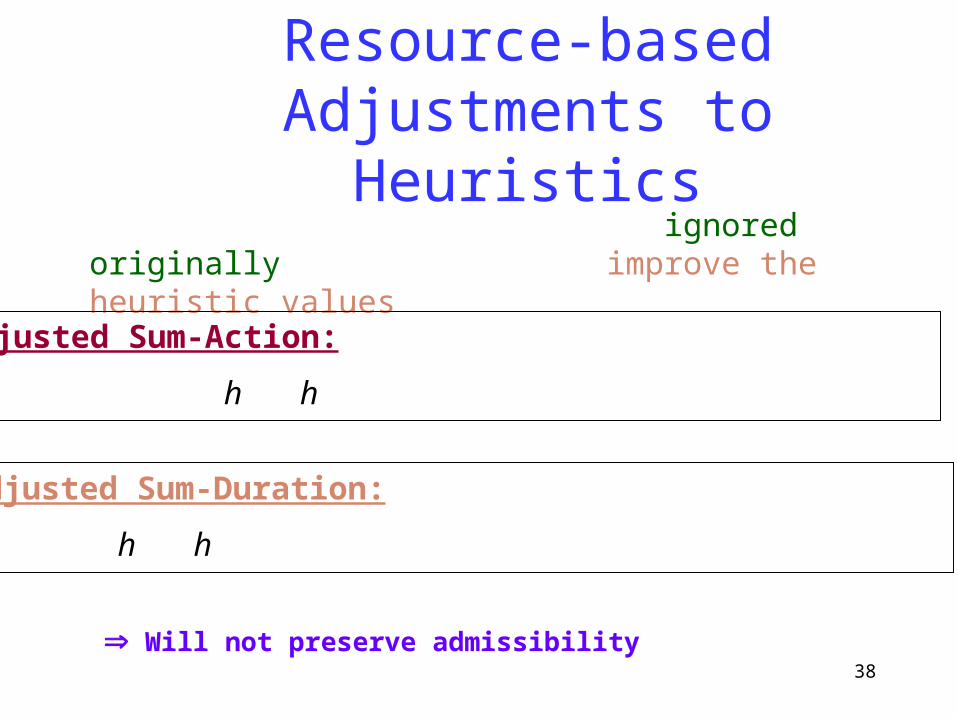
Resource-based Adjustments to Heuristics

Resource related information, ignored originally, can be used to improve the heuristic values

Adjusted Sum-Action:

h = h + R (Con(R) – (Init(R)+Pro(R)))/R

Adjusted Sum-Duration:

h = h + R [(Con(R) – (Init(R)+Pro(R)))/R].Dur(AR)

Will not preserve admissibility

39

The (Relaxed) Temporal PG

Tempe

Phoenix

Los Angeles

Drive-car(Tempe,LA)

Heli(T,P)

Shuttle(T,P)

Airplane(P,LA)

t = 0 t = 0.5 t = 1 t = 1.5 t = 10

40

Time-sensitive Cost Function

Standard (Temporal) planning graph (TPG) shows the time-related estimates e.g. earliest time to achieve fact, or to execute action

TPG does not show the cost estimates to achieve facts or execute actions

Tempe

Phoenix

L.A

Shuttle(Tempe,Phx): Cost: $20; Time: 1.0 hourHelicopter(Tempe,Phx):Cost: $100; Time: 0.5 hourCar(Tempe,LA):Cost: $100; Time: 10 hourAirplane(Phx,LA):Cost: $200; Time: 1.0 hour

cost

time0 1.5 2 10

$300

$220

$100

Drive-car(Tempe,LA)

Heli(T,P)

Shuttle(T,P)

Airplane(P,LA)

t = 0 t = 0.5 t = 1 t = 1.5 t = 10

41

Estimating the Cost Function

Tempe

Phoenix

L.A

time0 1.5 2 10

$300

$220

$100

t = 1.5 t = 10

Shuttle(Tempe,Phx): Cost: $20; Time: 1.0 hourHelicopter(Tempe,Phx):Cost: $100; Time: 0.5 hourCar(Tempe,LA):Cost: $100; Time: 10 hourAirplane(Phx,LA):Cost: $200; Time: 1.0 hour

1

Drive-car(Tempe,LA)

Hel(T,P)

Shuttle(T,P)

t = 0

Airplane(P,LA)

t = 0.5

0.5

t = 1

Cost(At(LA)) Cost(At(Phx)) = Cost(Flight(Phx,LA))

Airplane(P,LA)

t = 2.0

$20

42

Observations about cost functions

Because cost-functions decrease monotonically, we know that the cheapest cost is always at t_infinity (don’t need to look at other times) Cost functions will be monotonically decreasing as long as there are no exogenous

events Actions with time-sensitive preconditions are in essence dependent on exogenous

events (which is why PDDL 2.1 doesn’t allow you to say that the precondition must be true at an absolute time point—only a time point relative to the beginning of the action

If you have to model an action such as “Take Flight” such that it can only be done with valid flights that are pre-scheduled (e.g. 9:40AM, 11:30AM, 3:15PM etc), we can model it by having a precondition “Have-flight” which is asserted at 9:40AM, 11:30AM and 3:15PM using timed initial literals)

Becase cost-functions are step funtions, we need to evaluate the utility function U(makespan,cost) only at a finite number of time points (no matter how complex the U(.) function is. Cost functions will be step functions as long as the actions do not model

continuous change (which will come in at PDDL 2.1 Level 4). If you have continuous change, then the cost functions may change continuously too

ADDED

Not covered beyond this point..

44

Cost Propagation Issues:

At a given time point, each fact is supported by multiple actions Each action has more than one precondition

Propagation rules: Cost(f,t) = min {Cost(A,t) : f Effect(A)} Cost(A,t) = Aggregate(Cost(f,t): f Pre(A))

Sum-propagation: Cost(f,t) The plans for individual preconds may be interacting

Max-propagation: Max {Cost(f,t)} Combination: 0.5 Cost(f,t) + 0.5 Max {Cost(f,t)}

Probably other better ideas could be tried

Can’t use something like set-level idea here becauseThat will entail tracking the costs of subsets of literals

45

Termination Criteria

Deadline Termination: Terminate at time point t if: goal G: Dealine(G) t goal G: (Dealine(G) < t) (Cost(G,t) =

Fix-point Termination: Terminate at time point t where we can not improve the cost of any proposition.

K-lookahead approximation: At t where Cost(g,t) < , repeat the process of applying (set) of actions that can improve the cost functions k times.

cost

time0 1.5 2 10

$300

$220

$100

Drive-car(Tempe,LA)

H(T,P)

Shuttle(T,P)

Plane(P,LA)

t = 0 0.5 1 1.5 t = 10

Earliest time pointCheapest cost

46

Heuristic estimation using the cost functions

If the objective function is to minimize time: h = t0

If the objective function is to minimize cost: h = CostAggregate(G, t)

If the objective function is the function of both time and cost

O = f(time,cost) then:h = min f(t,Cost(G,t)) s.t. t0 t t

Eg: f(time,cost) = 100.makespan + Cost then h = 100x2 + 220 at t0 t = 2 t

time

cost

0 t0=1.5 2 t = 10

$300

$220

$100

Cost(At(LA))

Earliest achieve time: t0 = 1.5Lowest cost time: t = 10

The cost functions have information to track both temporal and costmetric of the plan, and their inter-dependent relations !!!

47

Heuristic estimation by extracting the relaxed plan

Relaxed plan satisfies all the goals ignoring the negative interaction: Take into account positive interaction Base set of actions for possible adjustment according to

neglected (relaxed) information (e.g. negative interaction, resource usage etc.)

Need to find a good relaxed plan (among multiple ones) according to the objective function

49

Heuristic estimation by extracting the relaxed plan

General Alg.: Traverse backward searching for actions supporting all the goals. When A is added to the relaxed plan RP, then:

Supported Fact = SF Effects(A)Goals = SF \ (G Precond(A))

Temporal Planning with Cost: If the objective function is f(time,cost), then A is selected such that:

f(t(RP+A),C(RP+A)) + f(t(Gnew),C(Gnew)) is minimal (Gnew = (G Precond(A)) \ Effects)

Finally, using mutex to set orders between A and actions in RP so that less number of causal constraints are violated

time

cost

0 t0=1.5 2 t = 10

$300

$220

$100

Tempe

Phoenix

L.A

f(t,c) = 100.makespan + Cost

50

Adjusting the Heuristic Values

Ignored resource related information can be used to improve the heuristic values (such like +ve and –ve interactions in classical planning)

Adjusted Cost:

C = C + R (Con(R) – (Init(R)+Pro(R)))/R * C(AR)

Cannot be applied to admissible heuristics

51

Partialization Example

A1 A2 A3

A1(10) gives g1 but deletes pA3(8) gives g2 but requires p at startA2(4) gives p at end We want g1,g2

A position-constrained plan with makespan 22

A1

A2

A3 G

p

g1

g2

[et(A1) <= et(A2)] or [st(A1) >= st(A3)][et(A2) <= st(A3)….

OrderConstrainedplan

The best makespan dispatch of the order-constrained plan

A1

A2 A3 14+

There could be multiple O.C. plansbecause of multiple possible causal sources. Optimization will involve Going through them all.

52

Problem Definitions Position constrained (p.c) plan: The execution time of each action is

fixed to a specific time point Can be generated more efficiently by state-space planners

Order constrained (o.c) plan: Only the relative orderings between actions are specified More flexible solutions, causal relations between actions

Partialization: Constructing a o.c plan from a p.c plan

QR R

G

QR

{Q} {G}

t1 t2 t3

p.c plan o.c plan

Q R RG

QR

{Q} {G}

53

Validity Requirements for a partialization

An o.c plan Poc is a valid partialization of a valid p.c plan Ppc, if: Poc contains the same actions as Ppc

Poc is executable Poc satisfies all the top level goals (Optional) Ppc is a legal dispatch (execution) of Poc

(Optional) Contains no redundant ordering relations

PQ

PQ

Xredundant

54

Greedy Approximations

Solving the optimization problem for makespan and number of orderings is NP-hard (Backstrom,1998)

Greedy approaches have been considered in classical planning (e.g. [Kambhampati & Kedar, 1993], [Veloso et. al.,1990]):

Find a causal explanation of correctness for the p.c plan Introduce just the orderings needed for the explanation to

hold

56

Modeling greedy approaches as value ordering strategies

Variation of [Kambhampati & Kedar,1993] greedy algorithm for temporal planning as value ordering: Supporting variables: Sp

A = A’ such that: etp

A’ < stpA in the p.c plan Ppc

B s.t.: etpA’ < etp

B < stpA

C s.t.: etpC < etp

A’ and satisfy two above conditions Ordering and interference variables:

pAB = < if etp

B < stpA ; p

AB = > if stpB > stp

A

rAA’= < if etr

A < strA’ in Ppc; r

AA’= > if strA > etr

A’ in Ppc; rAA’= other wise.

Key insight: We can capture many of the greedy approaches as specific value ordering strategies on the CSOP encoding

60

Empirical evaluation

Objective: Demonstrate that metric temporal planner armed with our

approach is able to produce plans that satisfy a variety of cost/makespan tradeoff.

Testing problems: Randomly generated logistics problems from TP4

(Hasslum&Geffner)Load/unload(package,location): Cost = 1; Duration = 1;Drive-inter-city(location1,location2): Cost = 4.0; Duration = 12.0;Flight(airport1,airport2): Cost = 15.0; Duration = 3.0;Drive-intra-city(location1,location2,city): Cost = 2.0; Duration = 2.0;

integrating planning & scheduling subbarao kambhampati integrating planning & scheduling...

Documents

planning scheduling

integration g

choice g

g talk

temporal planning slide

hsts operation scheduling

planning techniques

manugistics planning