benchmarking opex and capex in energy networks - accc home
TRANSCRIPT
Benchmarking Opex and Capex in Energy Networks
Working Paper no.6, May 2012
ACCC/AER WORKING PAPER SERIES

Benchmarking Opex and Capex in Energy Networks
ACCC/AER Working Paper No. 6, May 2012 ii
© Commonwealth of Australia 2012
ISBN 978-1-921964-51-0
This work is copyright. Apart from any use permitted by the Copyright Act 1968, no part may be reproduced without permission of the Australian Competition and Consumer Commission. Requests and enquiries concerning reproduction and rights should be addressed to the Director of Publishing, Australian Competition and Consumer Commission, GPO Box 3131, Canberra ACT 2601.
Citation details: ACCC/AER Working Paper 6 /May 2012
Series Note
The Australian Competition and Consumer Commission encourages vigorous competition in the marketplace and enforces consumer protection and fair trading laws, in particular the Competition and Consumer Act 2010 (formerly the Trade Practices Act).
The Australian Energy Regulator is an independent statutory authority and a constituent part of the ACCC.
Working papers are intended to disseminate the results of current research by ACCC staff and consultants. The aim of the series is to facilitate discussion and comment. The working papers come from across the ACCC covering competition law, economic regulation, and consumer protection. They are available at no cost in electronic format only from the ACCC website, www.accc.gov.au. To subscribe to this series, email [email protected]
The papers in this series reflect the views of the individual authors. The views expressed in the paper do not necessarily reflect the views of the ACCC or the AER.
Enquiries may be addressed to:
The Editor
ACCC/AER working paper series
Australian Competition and Consumer Commission
GPO Box 520
Melbourne Vic 3001
email: [email protected]

Benchmarking Opex and Capex in Energy Networks
ACCC/AER Working Paper No. 6, May 2012 1
Foreword
The working paper Benchmarking Opex and Capex in Energy Networks reviews five
alternative benchmarking methods – namely partial performance indicators, index-
number-based total factor productivity, econometric method, stochastic frontier
analysis, and data envelopment analysis – with a particular focus on their use in the
benchmarking and regulation of energy networks. The review covers published
studies from the academic literature and also consulting reports written for regulatory
purposes, as well as regulatory applications of benchmarking methods from 15 OECD
countries, including Australia, New Zealand, the United States, Canada, Japan and
various European countries (Austria, Denmark, Finland, Germany, Ireland, the
Netherlands, Norway, Spain, Sweden, and the United Kingdom).
The paper covers the key methods, relevant literature and regulatory practices, as well
as the major technical and implementation issues in benchmarking energy networks.
This provides a resource that will be of substantial benefit to regulatory analysts in
years to come. I found the various tables providing comprehensive and up-to-date
summaries of the wide range of empirical studies to be particularly valuable.
The document carefully lists the advantages and disadvantages of each benchmarking
method, in the context of regulation of energy networks. I was particularly pleased to
see the emphasis that was placed on obtaining good-quality data, since this is a key
prerequisite for any defendable benchmarking exercise. The majority of the data,
acquired during regulatory processes and practices, would be fundamental to future
benchmarking research.
Overall, I believe that this paper makes an important contribution to the current
discussion of the use of benchmarking for price regulation in energy networks in
Australia, and I hope that it will be widely read by stakeholders in Australia and
where ever benchmarking is being used in regulatory processes.
Tim Coelli
Adjunct Professor, School of Economics, University of Queensland
Economic Consultant (Associate), Economic Insights
Economic Consultant (Partner), Coelli Economic Consulting Services

Benchmarking Opex and Capex in Energy Networks
ACCC/AER Working Paper No. 6, May 2012 2
About the working paper
In November 2011, the Regulatory Development Branch of the Australian
Competition and Consumer Commission (ACCC) commenced a joint project with the
Australian Energy Regulator (AER), Benchmarking Opex and Capex in Energy
Networks. The project has a number of outputs, one of which is to be the sixth
working paper in the ACCC/AER series.
Because of the nature of the project being research-oriented, highly technical and
broad-ranging, this working paper draws upon contributions from a diversity of staff
with relevant knowledge and expertise. This paper also benefited from the insightful
thoughts provided by the external reviewer – Professor Tim Coelli, a distinguished
researcher in the efficiency and productivity field and one of the most highly cited
academic economists in Australia.
Of course final responsibility for the working paper rests with the ACCC/AER staff
working on this project. Dr Su Wu has led the overall project. The paper has evolved
from many rounds of drafting and revision by Dr Rob Albon, Dr Darryl Biggar, Dr
Hayden Mathysen and Megan Willcox, as well as a team of AER staff including Jess
Manahan, Cameron Martin, and Israel del Mundo. The finalisation of the working
paper also draws heavily on the reviewing contributions from Paul Dunn, Kylie
Finnin, Dr Jason King and Dr Anne Plympton.
The supporting research of regulatory practices in Australia and internationally draws
upon three separate pieces of work by WIK-Consult, Malcolm Tadgell from Utility
Regulation Services, and an internal research team led by Megan Willcox, with
assistance from Kylie Finnin, Jess Manahan, and Cameron Smith. Two outputs –
Regulatory Practices in Other Countries prepared internally and Cost Benchmarking
in Energy Regulation in European Countries prepared by WIK-Consult – are
published as reference documents.
Genevieve Pound has provided valuable editorial assistance.
For comments on this working paper, please contact the ACCC on this e-mail address:
It is hoped that this working paper will encourage further discussion about
benchmarking issues relevant to the ACCC/AER regulatory work.
Benchmarking Opex and Capex in Energy Networks
ACCC/AER Working Paper No. 6, May 2012 3
Table of contents
Foreword ........................................................................................................................ 1
About the working paper ............................................................................................... 2
Table of contents ............................................................................................................ 3
Synopsis ......................................................................................................................... 7
Chapter 1 Introduction and executive summary ....................................................... 8
1.1 Context ........................................................................................................... 8
1.2 Aim and purpose ............................................................................................ 9
1.3 Summary of findings.................................................................................... 10
1.3.1 Assessment of the benchmarking methods ............................................ 10
1.3.2 Lessons from regulatory practices ........................................................ 12
1.3.3 Concluding observations ....................................................................... 14
1.4 Structure of the paper ................................................................................... 15
Chapter 2 Evaluation of partial-performance-indicator method ............................. 16
2.1 Introduction .................................................................................................. 16
2.2 Description of the PPI method ..................................................................... 16
2.2.1 Method ................................................................................................... 16
2.2.2 Data requirement .................................................................................... 17
2.2.3 Advantages and disadvantages .............................................................. 17
2.3 Literature review of PPI method .................................................................. 18
2.4 Regulatory practices using PPI method ....................................................... 19
2.4.1 Regulatory practices review ................................................................... 19
2.4.2 Summary of regulatory practices ........................................................... 25
2.5 Issues arising from the review ..................................................................... 32
2.5.1 Limitations of PPI .................................................................................. 32
2.5.2 Legislative and regulatory requirements ................................................ 32
2.5.3 Industry characteristics .......................................................................... 33
2.5.4 Data availability and quality .................................................................. 33
2.5.5 The use of benchmarking results ........................................................... 34
2.6 Conclusions .................................................................................................. 35
Chapter 3 Evaluation of the index-number-based TFP analysis ............................ 36
3.1 Introduction .................................................................................................. 36
3.2 Description of the TFP method .................................................................... 37
3.2.1 Method ................................................................................................... 37
3.2.2 Data requirements .................................................................................. 39
Benchmarking Opex and Capex in Energy Networks
ACCC/AER Working Paper No. 6, May 2012 4
3.2.3 Advantages and disadvantages .............................................................. 41
3.3 Literature review of the TFP method ........................................................... 42
3.3.1 Literature review .................................................................................... 42
3.3.2 Summary of the studies .......................................................................... 45
3.4 Regulatory practices using the TFP method ................................................ 47
3.4.1 Regulatory practices review ................................................................... 47
3.4.2 Summary of regulatory practices ........................................................... 52
3.5 Issues arising from the review ..................................................................... 56
3.5.1 Data requirements .................................................................................. 57
3.5.2 Model specifications .............................................................................. 58
3.5.3 Applications ........................................................................................... 59
3.6 Conclusions .................................................................................................. 60
Chapter 4 Evaluation of the econometric approach to benchmarking.................... 61
4.1 Introduction .................................................................................................. 61
4.2 Description of the econometric approach to benchmarking ........................ 61
4.2.1 Method ................................................................................................... 61
4.2.2 Data requirements and selection of explanatory variables .................... 65
4.2.3 Advantages and disadvantages .............................................................. 67
4.3 Literature review of the econometric approach ........................................... 68
4.4 Regulatory practices using the econometric method ................................... 73
4.4.1 Regulatory practices review ................................................................... 73
4.4.2 Summary of regulatory practices ........................................................... 78
4.5 Issues arising from the review ..................................................................... 78
4.5.1 Choice of functional form ...................................................................... 78
4.5.2 Choice of explanatory variables............................................................. 79
4.5.3 Choice of estimation method ................................................................. 80
4.5.4 Interpretation of the results .................................................................... 82
4.6 Conclusions .................................................................................................. 82
Chapter 5 Evaluation of the parametric SFA method............................................. 84
5.1 Introduction .................................................................................................. 84
5.2 Description of the SFA method ................................................................... 84
5.2.1 Mathematical illustration ....................................................................... 85
5.2.2 Data requirements .................................................................................. 87
5.2.3 Advantages and disadvantages .............................................................. 89
5.3 Literature review of the SFA method .......................................................... 90
Benchmarking Opex and Capex in Energy Networks
ACCC/AER Working Paper No. 6, May 2012 5
5.3.1 SFA for primary analysis ....................................................................... 90
5.3.2 SFA for comparison with other benchmarking methods ....................... 92
5.3.3 SFA for sensitivity testing ..................................................................... 94
5.3.4 Data used in academic studies ............................................................... 95
5.3.5 Conclusion on literature review ............................................................. 95
5.4 Regulatory practices using the SFA method .............................................. 101
5.4.1 Regulatory practices review ................................................................. 101
5.4.2 Summary of regulatory practices ......................................................... 103
5.5 Issues arising from the review ................................................................... 103
5.5.1 Data requirements ................................................................................ 104
5.5.2 Required assumptions .......................................................................... 104
5.5.3 Limited regulatory applications ........................................................... 105
5.6 Conclusions ................................................................................................ 105
Chapter 6 Evaluation of the non-parametric DEA method .................................. 107
6.1 Introduction ................................................................................................ 107
6.2 Description of the DEA method ................................................................ 107
6.2.1 Method ................................................................................................. 107
6.2.2 Data requirements ................................................................................ 112
6.2.3 Advantages and disadvantages ............................................................ 113
6.3 Literature review of the DEA method ....................................................... 114
6.4 Regulatory practices using the DEA method ............................................. 125
6.4.1 Regulatory practices review ................................................................. 125
6.4.2 Summary of regulatory practices ......................................................... 130
6.5 Issues arising from the review ................................................................... 130
6.5.1 The choice of variables ........................................................................ 130
6.5.2 The specification of the DEA model ................................................... 133
6.5.3 Importance of data quality ................................................................... 133
6.5.4 Validation of a DEA model ................................................................. 134
6.6 Conclusions ................................................................................................ 135
Chapter 7 Common issues in benchmarking of energy networks ........................ 136
7.1 Introduction ................................................................................................ 136
7.2 Summary of alternative benchmarking methods ....................................... 136
7.3 Data issues in benchmarking ..................................................................... 141
7.3.1 General data requirements ................................................................... 141
7.3.2 Potential data problems ........................................................................ 141
Benchmarking Opex and Capex in Energy Networks
ACCC/AER Working Paper No. 6, May 2012 6
7.4 Model specification issues ......................................................................... 142
7.4.1 Model specifications ............................................................................ 142
7.4.2 Output specification and measurement ................................................ 144
7.4.3 Input specification and measurement ................................................... 145
7.4.4 Cost measures ...................................................................................... 147
7.4.5 Operating environment factors ............................................................ 147
7.4.6 Functional forms .................................................................................. 148
7.5 Insights into benchmarking of energy networks ........................................ 149
7.5.1 Addressing potential data issues .......................................................... 149
7.5.2 Addressing model specification problems ........................................... 151
7.5.3 Choice of methods ............................................................................... 152
7.6 Conclusions ................................................................................................ 154
Chapter 8 Implementation issues in achieving effective benchmarking .............. 155
8.1 Introduction ............................................................................................... 155
8.2 Operating expenditure, capital expenditure and total expenditure and their
tradeoffs ..................................................................................................... 155
8.3 The consideration of service quality and reliability ................................... 160
8.4 Benchmarking: an informative tool and a deterministic tool ..................... 162
8.5 Implementation process ............................................................................. 165
8.6 Benchmarking: opportunities and possibilities .......................................... 165
References .................................................................................................................. 170
Abbreviations ............................................................................................................. 184
Benchmarking Opex and Capex in Energy Networks
ACCC/AER Working Paper No. 6, May 2012 7
Synopsis
This paper reviews different benchmarking techniques that may be applied to a cost
assessment of energy networks, particularly electricity and gas distribution
businesses, under the regulatory determinations.
The purpose of cost benchmarking is to improve cost efficiency in the operation of
energy networks and to assist in achieving the legislative goals set for the economic
regulators. In this paper, benchmarking is broadly defined as the comparison of a
utility’s performance with some pre-defined reference performance (see for example,
Jamasb and Pollitt, 2001, p. 108), such as its past performance (e.g., trend analysis) or
best-practice or average performance of similar entities in the country or in the world.
Five benchmarking methods are reviewed:
Partial Performance Indicator (PPI) method;
Index-number-based Total Factor Productivity (TFP) analysis;
Econometric method (EM);
Stochastic Frontier Analysis (SFA); and
Data Envelopment Analysis (DEA).
Each of the methods is covered in a method-based chapter containing: a discussion of
the respective benchmarking method; a review of the literature in relation to that
method; a survey of international regulatory practices that have employed that
method; and a section setting out key issues regarding use of the method.
After this review has been undertaken, common analytical and empirical issues in cost
benchmarking of energy networks are identified. Issues associated with
implementation of cost benchmarking for regulatory purposes are examined in a final
chapter.
Benchmarking Opex and Capex in Energy Networks
ACCC/AER Working Paper No. 6, May 2012 8
Chapter 1 Introduction and executive summary
1.1 Context
The search for better ways of regulating energy utilities has increasingly included
‘cost benchmarking’, where the reasonableness of costs proposed is assessed against
those of other utilities or even against costs estimated in economic-engineering
models. Benchmarking has been applied in a large and increasing number of
countries across the Organisation for Economic Cooperation and Development
(OECD) in relation to both operating expenditure (opex) and capital expenditure
(capex); particularly for distribution service operators in both the electricity and gas
sub-sectors.
In Australia, there has long been interest in this approach, stretching back at the state
level to the late 1990s. Currently the Australian Energy Regulator (AER) must have
reference to the costs of an ‘efficient operator’ in a revenue or price determination.
Further, interest in benchmarking has been heightened recently by two major
inquiries; one by the Productivity Commission (PC) on benchmarking;1 and the other,
by the Australian Energy Market Commission (AEMC), in relation to proposed rule
changes.2
The AEMC’s investigation commenced in October 2011 and includes consideration
of requests from the AER and the Energy Users’ Rule Change Committee. The
AER’s proposals relate to ‘changes to the capital and operating expenditure
frameworks’ and ‘changes to the expenditure incentive arrangements’. Many
submissions have raised the benchmarking issue. The PC’s inquiry (commenced
January 2012) is particularly apposite (Swan, 2012, paragraph 3):
The purpose of the inquiry is to inform the Australian Government about whether there are
any practical or empirical constraints on the use of benchmarking of network businesses
and then provide advice on how benchmarking could deliver efficient outcomes, consistent
with the National Electricity Objective (NEO).
The reason for this heightened interest in benchmarking is clear. Efficient energy
production and pricing are vital to the efficient functioning of a developed economy
operating in an internationally competitive environment. Ultimately, the prices paid
by end users for energy primarily depend on the underlying costs of production. Both
electricity and gas are produced using sophisticated supply chains, and elements of
these supply chains exhibit, to greater and lesser extents, natural monopoly
characteristics such as economies of scale, economies of scope and economies of
density. In turn, these features militate against competition – natural monopoly means
that duplication of production facilities will fracture these economies, resulting in
higher-than-necessary production costs. On the other hand, production by a
single entity gives rise to market power which could be exploited to the detriment of
end users and to economic efficiency.
1 For background information, see the Productivity Commission’s website at:
http://www.pc.gov.au/projects/inquiry/electricity [accessed on 22 December 2011] and Productivity
Commission (2012). 2 For proposals and submissions, see the AEMC’s website at:
http://www.aemc.gov.au/Electricity/Rule-changes/Open/Economic-Regulation-of-Network-Service-
Providers-.html [accessed on 22 December 2011].

Benchmarking Opex and Capex in Energy Networks
ACCC/AER Working Paper No. 6, May 2012 9
Across the OECD countries, it is common for governments to operate regulatory
regimes aimed at producing more efficient outcomes than the unrestrained market. In
Australia, as in most OECD countries, efficiency is interpreted broadly to include the
‘trilogy’ of economic efficiencies – cost efficiency (encompassing production
efficiency, technical efficiency and X-efficiency, meaning producing output at the
least cost); allocative efficiency (relating prices to underlying costs to minimise
deadweight loss); and dynamic efficiency (encouraging innovation of new
technologies and production methods) (see ACCC/AER, 2010). These efficiency
criteria underlie both the National Electricity Law (NEL) and the National Gas Law
(NGL). They date back to the Hilmer reforms of the early nineties (Independent
Committee of Inquiry into National Competition Policy, 1993), and pervade all of
Australia’s infrastructure regulation.
Excessive production costs can arise in a variety of ways, and the concept of ‘cost
inefficiency’ has a number of interpretations. For example, a producer's input choice
can be distorted by a tax on a particular input produced in a competitive upstream
market, forcing it to use less of that input and more of other inputs to produce a given
level of output, resulting in wasteful input use and higher-than-necessary economic
costs. Other interventions, such as input subsidies and restrictions on input use, can
have similar effects on production costs. There are other reasons why producers
might be using an inefficient mix of inputs and/or too many inputs to produce
outputs. For example, Hicks (1935) referred to the ‘easy life’ as an objective of
management, where monopoly power can be enjoyed through the avoidance of
difficult decisions about cost minimisation (e.g., maintaining over-staffing); and
Leibenstein (1987) introduced the term ‘X-inefficiency’ to describe situations where
management adopts a stance of producing with too many inputs.
Some regulatory approaches may also discourage cost minimisation. In particular, the
traditional approach to infrastructure regulation in the United States is described
either as ‘rate-of-return regulation’ or ‘cost-of-service regulation’, and could involve
one or both of the distortion of input choice (the ‘Averch-Johnson effect’; Averch and
Johnson, 1962) and ‘cost padding’ (Albon and Kirby, 1983) in lieu of monopoly
profits. Cost inefficiency can also be associated with the ‘building-block model’
approach practised in Australia, where there is limited or unsuccessful scrutiny of
capex and opex levels proposed by regulated entities. As a consequence, excessive
costs may be built into the prices of electricity and gas to end users.
1.2 Aim and purpose
Five benchmarking methods are examined by providing an extensive review of:
academic literature; and
regulatory applications of benchmarking techniques across selected countries.
This includes a review of academic papers, research reports and consultancy reports
with a focus on the different methods used to assess costs and/or efficiency and
productivity performance of networks operating in the electricity and gas sub-sectors.
This paper considers the theoretical basis for the use of each method for
benchmarking. Data and model requirements are considered, as well as the strengths
Benchmarking Opex and Capex in Energy Networks
ACCC/AER Working Paper No. 6, May 2012 10
and weaknesses of each statistical method. Key issues arising in the literature are
identified and summarised.
The review of regulatory practice consists of 15 OECD countries: Australia, Austria,
Canada (Ontario), Denmark, Finland, Germany, Ireland, Japan, the Netherlands, New
Zealand, Norway, Spain, Sweden, the United Kingdom and the United States
(California).3 The review covers most of the leading countries, including the largest
of these and many smaller countries. It reviews techniques used, modelling
undertaken, data availability, results and processes of implementation. For Australia,
benchmarking applications by both the AER and the state and territory regulators (in
performing their roles in energy network regulation preceding the transfer of
regulatory responsibilities to the AER) are reviewed. For Canada and the United
States, the scope of the review is limited to relevant practices by the Ontario Energy
Board and the California Public Utilities Commission, as an example of regulatory
applications in these two countries.
Based on the review, the paper attempts to draw out guidance for economic regulators
in their pursuit of better regulation of transmission and distribution networks in
electricity and gas. This guidance relates to the particular techniques and approaches
that are most promising; the data and model specification issues that arise in applying
these techniques including issues such as adjustments for factors beyond the regulated
entity’s control; and the processes that could be followed in applying cost
benchmarking.
1.3 Summary of findings
Findings consist of:
an assessment of the benchmarking methods;
lessons from regulatory practices; and
concluding observations.
1.3.1 Assessment of the benchmarking methods
This paper systematically reviews five benchmarking methods, namely Partial
Performance Indicator (PPI) method, Index-number-based Total Factor Productivity
(TFP) analysis, Econometric method (EM), Stochastic Frontier Analysis (SFA); and
Data Envelopment Analysis (DEA).
In summary:
There is a large range of data requirements reflecting differences in the
comprehensiveness and accuracy of methods arrayed along the spectrum of
simplicity to complexity. PPI has limited data requirements while TFP is
information-intensive as it requires both price and quantity information on
3 A large part of the work has been conducted internally and documented in a supporting reference
document titled ‘Regulatory Practices in Other Countries’ (ACCC/AER, 2012). The work has also
been enhanced by a consultancy report on ‘Cost Benchmarking in Energy Regulation in European
Countries – Final Report’ prepared by WIK-Consult (WIK-Consult, 2011). The report provides
information on several non-English-speaking European economies.
Benchmarking Opex and Capex in Energy Networks
ACCC/AER Working Paper No. 6, May 2012 11
inputs and outputs. Between the two ends of the spectrum, the other three
methods (EM, SFA and DEA) are more effective the larger the number of
observations in the sample.
PPI analysis calculates a single explanatory variable and therefore requires less
data than other approaches. Results obtained by PPI may suggest that
significant cost differences exist between businesses. However, PPI can only
provide a partial indication of performance and is not able to separately account
for multiple inputs. This approach may have a role in conjunction with other
methods.
Index-number-based TFP accommodates multiple inputs and outputs. While
this differentiates it favourably from the PPI method in terms of capturing the
overall picture, there are a number of challenges. First, it requires a large
amount of high-quality data. Second, there may be conceptual issues in
determining the capital input. Third, it is difficult to directly incorporate
quality-of-services into the analysis. Fourth, it is a non-parametric technique.
This means that statistical testing cannot be performed. With respect to
regulatory use, TFP is more commonly used in the regulatory practices to
inform industry-wide productivity change. Other methods are more often used
to inform comparative performance.
SFA is the most complete approach that is relatively strong on both theoretical
and statistical grounds. By modelling all relevant inputs and outputs and
explicitly including a stochastic element for statistical testing, it can provide
additional insights into the significance of key cost drivers and the role of
technology over time. A shortcoming of the conventional econometric method,
compared with SFA, is that it does not separate the inefficiency measure of the
businesses from ‘noise’ in the data. This makes interpretation of the estimated
residual difficult. Nevertheless, with careful examination of data and selection
of model specifications and estimation methods, this method has the potential to
provide important insights.
DEA is a relatively simple technique, which has been widely applied in
academic literature and regulatory practice. However, as a deterministic
method, DEA results are sensitive to the presence of outlying observations.
The following technical and application issues in relation to cost benchmarking arise
from the review of the literature:
The selection of the input-output specification and functional form should be
informed by a combination of sound economic theory, good engineering
knowledge and rigorous ‘cost driver’ analysis.
In principle it is preferable to compare the total expenditure across businesses.
However, this requires an assessment of the consumption of the volume of
capital services in a period (or an allocation of the total capital expenditure to
that period). There are conceptual issues in carrying out that assessment or
allocation. As a consequence, many regulators put aside capital expenditure and
compare operating expenditure across businesses. This may create incentives

Benchmarking Opex and Capex in Energy Networks
ACCC/AER Working Paper No. 6, May 2012 12
for businesses to substitute between capital expenditure and operating
expenditure.
Effective benchmarking requires the modelling of relevant factors affecting the
expenditure of the energy networks. These businesses provide a range of
services using different types of inputs and may operate in different
environmental conditions. Inevitably, benchmarking requires some aggregation
of those services, inputs, or environmental conditions into a few variables,
resulting in some degree of approximation in the estimation.
Given the need to use a large dataset for benchmarking, panel-data analysis and
international benchmarking can be potentially helpful.
Where the choice of benchmarking methods and model specifications cannot be
settled on theoretical grounds, it may be useful to apply more than one technique
or model specification to test consistency. However, academic studies have
found that different benchmarking techniques do not exhibit a very high degree
of mutual consistency. In some cases, the inability to produce similar results
with alternative model specifications and methods require further investigation
so that benchmarking outcomes can be supported by more rigorous analysis.
It is critical to control for exogenous influences beyond the control of the
regulated business (‘environmental noise’). That is, it is important to consider
the role of exogenous environmental factors that are out of management control
but may influence the comparative cost performance. Depending on the
benchmarking method(s) selected, either one-step or two-step analysis can be
conducted to remove the impact of those exogenous influences (Yu, 1998).
1.3.2 Lessons from regulatory practices
The following general observations emerge from a review of regulatory practices
across 15 OECD jurisdictions where important applications of benchmarking have
been adopted:
Cost benchmarking methods have been employed by numerous international
energy regulators to analyse the efficiency of the electricity distribution
sub-sector for the purposes of regulatory determinations. To a lesser extent, cost
benchmarking has been employed in relation to the gas distribution sub-sector
and only a few energy regulators appear to have employed cost benchmarking to
analyse the energy transmission sub-sectors.
All five methods have been used in at least three of the jurisdictions examined:
PPI or unit-cost benchmarking methods have been used in Ireland, the
United Kingdom, the Netherlands, New Zealand, in Ontario, Canada and
by the AER and other Australian energy regulators.
Index-number-based TFP methods have been used in New Zealand,
Germany, Austria, in Ontario, Canada and in some states (e.g.,
California) in the United States, and by the Northern Territory Utilities
Commission in Australia.
Benchmarking Opex and Capex in Energy Networks
ACCC/AER Working Paper No. 6, May 2012 13
Econometric methods have been used in Austria, the United Kingdom,
Ireland, as well as in Ontario, Canada, and California, the United States.
SFA has been used in Germany, Finland, and Sweden.
DEA has been applied in Finland, Norway, the Netherlands, Germany,
Austria, and by the Independent Pricing and Regulatory Tribunal of New
South Wales (IPART) in Australia.
Some regulators have analysed energy networks using a number of
benchmarking techniques. For example, the German regulator used DEA and
SFA to determine the comparative performance of gas and electricity
distribution networks. It also relied on an index-number-based TFP method to
determine the productivity change common to all networks. Some regulated
utilities in the United States have submitted index-number-based TFP studies to
support their preferred value of the productivity-offsetting factor under a CPI–X
price/revenue path. The econometric method may also be employed in this
context to support the primary analysis.
Benchmarking has only recently been adopted in many European countries.
This coincides with the recent introduction of incentive-based regulation in
these countries. From those reviewed by WIK-Consult (2011): Norway was the
first to introduce incentive regulation and efficiency benchmarking in 1997;
Austria commenced in 2006; Finland in 2008; and Germany in 2009. Sweden
will move from a reference network model to ex ante revenue caps in 2012.
In North America, voluntary participation in benchmarking studies by regulated
energy utilities is popular. This provides businesses with an insight into how
they can improve their own performance relative to their peers. Some have used
these studies to support requests to the regulator for tariff reviews (First Quartile
Consulting, 2010).
The review of international regulatory practices shows that stakeholders and
regulators appear to be more confident with the use of cost benchmarking in
circumstances where:
there was extensive consultation with industry and the views of industry were
incorporated into the benchmarking regime where reasonable argument was
provided. For example, the Ofgem’s application of benchmarking to electricity
distribution included an extensive consultation process over a number of years.
benchmarking was used as a routine part of the regulatory process to inform the
regulatory decisions. That is where benchmarking was used to adjust the
business’s forecast costs up and down, rather than including the numerical
outputs from benchmarking directly into the determination of efficient costs or
X factors. Examples of this approach undertaken by the regulators include the
gas and electricity distribution sub-sectors in the United States, the United
Kingdom and Ireland.
there are a large number of comparable businesses in the sample. Regulators
have generally placed less weight on the results from benchmarking studies

Benchmarking Opex and Capex in Energy Networks
ACCC/AER Working Paper No. 6, May 2012 14
where there is a small sample size. For example, Ireland has only two gas
networks and the United Kingdom has eight networks owned by four
companies. Because of the limited sample size available, benchmarking
analyses of gas distribution networks in the United Kingdom (and Ireland, if
applicable) have been used in combination with bottom-up assessments of
specific activities to inform the regulators’ determinations of efficient costs. In
contrast, of the European countries reviewed by WIK-Consult (2011), Germany
and Austria have heavily relied on benchmarking results in their respective
regulatory decisions for gas distribution.4
multiple benchmarking techniques are used and considered. To account for the
different results that may arise using different methods, Finland and Germany
combined the results from the SFA and DEA methods, Austria combined results
of DEA and Modified Ordinary Least Squares (MOLS) and the Ontarian
regulator combined the results of econometric and unit-cost models. Finally, the
Ofgem in the United Kingdom compared the ranking of electricity distribution
networks derived from OLS and DEA methods to test the sensitivity of the
results.
1.3.3 Concluding observations
A key message from the review is that cost benchmarking is most effectively pursued
as an integral part of the broad regulatory process. Use of cost benchmarking would
move from being mainly an informative tool to being a deterministic tool through the
built-up of expertise (including learning by doing) and the gathering of necessary
resources.
Reflecting current practice and existing expertise, benchmarking should initially be
used as an informative tool rather than a determinative one. For example, it can be
used as a starting point for a conversation with regulated utilities about the level of
operating and/or capital expenditures being incurred and proposed. A more
sophisticated application could emerge over time.
Effective cost benchmarking requires a clear understanding of the structure of the
costs of the regulated utilities. This, in turn, requires an understanding of the key
outputs provided by the benchmarked utilities, the inputs used (and/or the prices of
those inputs), and the key environmental factors. It is also useful to understand the
nature of any economies of scale or scope in the industry. Engineering studies can
help provide a picture of the likely cost drivers, including how the cost drivers
interact. This involves complementing in-house resources through access to expert
consultants with specialised engineering knowledge and experience in the application
of cost-benchmarking methods.
The effectiveness of the use of more sophisticated techniques will be greater, the
greater the availability of relevant data. Achieving this will likely require the
investigation of international datasets if the number of regulated utilities in a sub-
sector is small. A key step is to identify compatible international data that are
4 The Austrian regulator has relied primarily on benchmarking results to determine the X factors,
supplemented by engineering studies to inform model specifications for benchmarking 20 gas
distribution businesses in the country. For more details, see WIK-Consult (2011).
Benchmarking Opex and Capex in Energy Networks
ACCC/AER Working Paper No. 6, May 2012 15
available and to understand the issues that arise when using international data to
benchmark domestic utilities. Accessing and understanding the limitations of data
from other countries or jurisdictions is likely to involve cooperation with regulators in
the relevant jurisdictions.
For cost-benchmarking applications, it is important to ensure that there are no
artificial incentives that create cost inefficiency through one or more of cost padding
(such as expense preferencing and empire building); pursuit of the ‘quiet life’ (such as
acquiescing to labour demands) and substitution of capital expenditure for operating
expenditure.
1.4 Structure of the paper
The remainder of this paper is structured as follows. Chapters 2 to 6 each reviews a
benchmarking method – namely PPI, TFP, EM, SFA and DEA – each chapter
covering a method description, literature review, regulatory applications, and issues
arising from the review. Chapter 7 considers common issues in benchmarking of
energy networks and Chapter 8 examines implementation issues in achieving effective
regulation using benchmarking.
Benchmarking Opex and Capex in Energy Networks
ACCC/AER Working Paper No. 6, May 2012 16
Chapter 2 Evaluation of partial-performance-indicator method
2.1 Introduction
Partial-performance-indicator (PPI) method involves the use of trend or ratio analysis
on part (but not all) of a business’s inputs or outputs to allow judgements or
comparisons to be made on some aspects of the productivity or efficiency
performance of comparable businesses or an industry average.
PPI has been used as a means of benchmarking the performance of gas and electricity
utilities by various international energy sector regulators, including in the United
Kingdom (UK), New Zealand, the Netherlands and Ontario, Canada. PPI has also
been used by Australian regulators including the AER and state jurisdictional
regulators.
While PPI has been commonly used by regulators in Australia and internationally, its
use in energy regulation has not been explored in the academic literature to any great
extent. The academic literature on benchmarking in the energy sector relates mostly
to the more complex techniques such as SFA, DEA, index-number-based TFP and
econometric methods. However, there is some literature relating to PPI measures,
which is outlined in this chapter.
The remainder of this chapter is structured as follows: A description of PPI is
provided in section 2.2. Section 2.3 provides a summary of the academic literature
relating to PPI method and section 2.4 provides a summary of the use of PPI by
energy regulators. Section 2.5 discusses some of the issues associated with the
application of PPI and conclusions are drawn in section 2.6.
2.2 Description of the PPI method
PPI method is carried out by calculating different measures of the financial, operating
and quality-of-services performance of comparable businesses. In terms of efficiency
and productivity performance, commonly adopted measures include:
single input factor productivity measures in terms of labour, capital stock,
material and/or fuel respectively; and
unit-cost measures, such as average total costs (total costs divided by a single
measure of output).
2.2.1 Method
At a basic level, PPI can be expressed in the following terms:
measureoutputmeasureinputPPI (2.1)
The key assumptions of the PPI measure is that a linear relationship exists between
the input and output measured and that any change in the input can be explained by a
change in the output (or vice versa).
In electricity distribution, the input measure may represent a single input, such as the
cost of clearing vegetation, or a more aggregated measure, such as opex or capex. The
Benchmarking Opex and Capex in Energy Networks
ACCC/AER Working Paper No. 6, May 2012 17
output measure is usually represented by a measure such as network length, power
delivered, customer numbers or customer density.
2.2.2 Data requirement
PPI measurements can be carried out using any measure of input and output, from
aggregated measures of opex or capex, down to individual business activities to
model. The data requirements depend on what the regulator is seeking to benchmark
(e.g. opex, capex, a component of opex, etc) and the level of information
disaggregation required. For example, benchmarking that is carried out on
expenditure relating to clearing vegetation will require a greater level of
disaggregated information than if benchmarking is carried out on total opex. The key
requirement is that, for any given input or output, the data collected must be measured
on a consistent basis across businesses. If data are not collected on a consistent basis,
then any comparison or benchmarking carried out using the data is likely to be
flawed.
2.2.3 Advantages and disadvantages
The indicators produced through PPI are generally easy to compute and simple to
interpret. They are also widely used by the industry, regulators and practitioners.
They can be used to compare certain aspects of efficiency and productivity
performance. Comparisons could be made either across different businesses at a
single point in time (i.e., cross-sectional analysis based on a sample of peers in the
group) or across time for the same business or industry (i.e., time-series analysis) or
both (i.e., panel-data analysis). The analysis can help identify trends, determine
baselines and establish target performance.
While PPIs provide some insights, they can give misleading information regarding the
overall economic performance of energy utilities producing multiple outputs and
multiple inputs. For example, when considered in isolation, a labour productivity
measure would tend to overstate the growth of overall productivity in a utility
experiencing a substantial degree of capital deepening (i.e., capital substituting for
labour in the production). Similarly, inadequately accounting for the multiple outputs
produced by a utility would also make performance comparison over time or across
utilities less useful for the regulator.
PPIs assume a linear relationship between the input and output measures and also
assume that any change in the input measure can be described by a change in the
output measure. However, in most circumstances the change in an input usage will be
dependent on a number of inputs, outputs and other factors that may not be described
in the model. In particular, PPIs used in isolation cannot easily take into account
differences in the market or operating environment that impact upon a business but
are beyond the control of management. For example, a utility may have a relatively
high or low unit cost simply because it faces input prices or serves customers that are
different from those for utilities operating in other regions. Because of this, they may
present problems in providing a meaningful comparison of businesses in different
operating environments.
The use of a matrix of partial performance measures to compare performance of
utilities, grouped by scale of operation (such as a composite scale variable), customer
Benchmarking Opex and Capex in Energy Networks
ACCC/AER Working Paper No. 6, May 2012 18
type or density, network density, capital density, or a combination of these, often
leads to the identification of different best and worst performers in the different
dimensions. A weighted-average performance indicator to combine a set of core
performance measures also raises some potential problems because the choice of
weights may be arbitrary and the overall indicator may fail to account for differences
in the operating environment. These problems suggest a need for a method to derive
comprehensive performance measures that can capture all the information on the
inputs used and outputs produced (and thus take into account potential trade-off
among outputs and inputs) and that can adjust for differences in non-controllable
factors that may affect utility performance.
2.3 Literature review of PPI method
In spite of the common use of PPI method by energy regulators, literature relating to
the regulatory use of PPI method is fairly limited. The limited amount of academic
attention paid to PPI applications to energy regulation may be a result of the relatively
simple nature of the method and potentially a preference amongst academics and
researchers to utilise a more advanced benchmarking technique that is capable of
giving a unified measure of productivity or efficiency, rather than a method based on
partial performance.
London Economics (1999) was somewhat negative in its assessment of PPI as a
means of efficiency analysis, noting that ‘while partial performance indicators can
provide useful insights into particular areas of inefficiency, they cannot provide an
overall picture of performance. Indeed, used by themselves, partial performance
indicators can provide a distorted picture of performance.’ (p. 7). The paper
considered that, for electricity distribution with multiple inputs and multiple outputs,
it was difficult to interpret the set of individual partial performance indicators required
to capture the different dimensions of the performance of the activities (London
Economics, 1999, p. 7).
Carrington, Coelli and Groom (2002, pp. 196-197) considered that ‘partial
productivity measures are often used to measure efficiency because they are simple to
calculate and are readily understood’. However, they further noted that ‘partial
productivity measures need to be implemented with care. The measures do not
provide a complete view of performance because they do not consider the various
relationships or trade-offs between inputs and outputs of gas distribution.
Furthermore, they can vary for reasons other than inefficiency; for example, a
distributor may have a different mix of customers or population density.’
Costello (2010, p. 44) pointed out that accounting indicators allow the user to identify
potential problem areas, provide preliminary information for in-depth inquiry and
allow a comparison of a utility's performance over time or with other utilities.
However, he also recognised many shortcomings of the method. For example, it does
not allow for the separation of management effects from other factors of performance;
and narrow-based measures may not account for interdependencies between utility
functions, and do not provide a definite benchmark.
Noting the common use of PPIs by Australian regulators to examine many different
aspects of the efficiency of regulated distribution utilities, Cambridge Economics
Policy Associates (CEPA) (2003, pp. 25-26) warned that partial productivity
Benchmarking Opex and Capex in Energy Networks
ACCC/AER Working Paper No. 6, May 2012 19
measures can be highly misleading as they are often significantly impacted by capital
substitution effects (where capital is substituted for labour, therefore improving labour
productivity). According to CEPA (2003), the main problem with these measures is
that it is not clear what can be done with them. For example, there is no meaningful
way of summing up the different efficiency savings given by PPIs to give a measure
of overall efficiency savings that could be achieved. CEPA (2003) also noted that the
partial approach neglects the fact that companies may choose to substitute one type of
expenditure for another, hence giving them best performance on some measures but
not on others, leaving best performance on all measures simultaneously unachievable.
CEPA (2003) indicated a preference for TFP indices to PPI because the TFP method
gives a more balanced view of efficiency and productivity performance. However,
the paper did evaluate both the advantages and disadvantages of PPI. The advantages
of PPI include that it is easy to compute and understand and can be used to cross
check results from more advanced benchmarking techniques such as Data
Envelopment Analysis (DEA) and Corrected Ordinary Least Squares (COLS) for
plausibility and transparency. The disadvantages of PPI include: no allowance for
evaluation of uncertainty associated with calculating benchmarks; difficulties in
accounting for differences in operating environments between businesses; potentially
misleading results by focussing on a subset of factors of production; and failure to
give an overall measure of potential for cost improvement that is supported by a
strong theoretical rationale.
2.4 Regulatory practices using PPI method
2.4.1 Regulatory practices review
PPI benchmarking method has been used as part of revenue or price determinations
for electricity and gas distribution networks by energy regulators in Australia and
some other countries, such as Ireland, the United Kingdom, the Netherlands, New
Zealand and Canada.5
Ireland6
Ireland’s energy regulator, the Commission for Energy Regulation (the CER), utilised
PPI methods to inform revenue decision for its single electricity distribution business,
ESB Network (ESBN), for the period 2011 to 2015. PPI analysis was carried out on
certain categories of opex (bottom-up analysis) and the results were considered in
conjunction with the results of total opex benchmarking (top-down analysis) based on
econometric methods (refer section 4.4).
The CER engaged the services of an engineering and technical consultant, Sinclair
Knight Merz, to carry out the PPI benchmarking. Sinclair Knight Merz considered it
possible to benchmark certain costs directly where costs are mainly fixed costs or
where a simple driver can be identified.
5 As it is not possible to cover all countries, there may be other examples of energy regulators applying
PPI benchmarking method that have not been captured in this paper and the supporting research.
Haney and Pollitt (2009) also undertook an international survey of benchmarking applications by
energy regulators. 6 Refer to chapter three of ‘Regulatory Practices in Other Countries’ (ACCC/AER, 2012).
Benchmarking Opex and Capex in Energy Networks
ACCC/AER Working Paper No. 6, May 2012 20
PPI benchmarking was carried out in relation to:
tree-cutting costs per network kilometre and tree coverage per kilometre;
fault costs per network kilometre; and
IT/Telecoms costs and System Control support costs per annum.
The benchmarks used for Ireland’s ESBN were 14 electricity distribution businesses
in the UK.
Sinclair Knight Merz noted that bottom-up PPI benchmarking indicates that some
repairs and maintenance costs in Ireland are inherently lower than in the United
Kingdom. The ESBN’s overhead line networks are simple and there is less urban
cable network. Sinclair Knight Merz considered that the real country differences in
terms of networks, practices and costs were beginning to be understood. Sinclair
Knight Merz, however, advised that its benchmarking results should be used with
caution. It was noted that identifying inefficiency of ESBN through international
benchmarking was becoming more difficult due to the narrowing efficiency gap and
the absence of detailed knowledge of cost allocations and network characteristics.
Based on the advice, the CER questioned whether benchmarking against distribution
businesses in the UK was applicable to Ireland which has four times more lines than
the UK companies of the same customer base. Nevertheless, the CER, taking into
account both the bottom-up and top-down benchmarking, adopted most of Sinclair
Knight Merz’s recommendations and reduced ESBN’s controllable opex costs.
ESBN has also taken advantage of the benchmarking information, which led to the
review of maintenance practices and PAS 55 asset management accreditation under
the auspices of the accreditation authority for the UK (Sinclair Knight Merz, 2010,
p. 29).7
United Kingdom8
The UK energy regulator, Ofgem, determined the revenue allowance for its eight gas
distribution networks (under four ownership groups) for the regulatory period
2008-09 to 2012-13. The Ofgem’s consultant LECG utilised PPI benchmarking
methods for benchmarking indirect opex. PPI benchmarking was undertaken at the
ownership level and included actual and forecast costs data between 2005-06 and
2012-13. Data from earlier periods could not be incorporated into the analysis due to
significant industry restructuring in 2005-06 which affected the data consistency
across time.
PPI benchmarking was carried out separately in relation to:
total support costs, finance and audit costs, legal costs, information systems
costs and insurance costs (each as a percentage of adjusted revenue);
7 PAS 55 is the British Standards Institution’s (BSI) Publicly Available Specification (PAS) for the
optimised management of physical assets – it provides clear definitions and a 28-point requirements
specification for establishing and verifying a joined-up, optimised and whole-life management system
for all types of physical assets. More information can be obtained at http://pas55.net. 8 Refer to chapter two of ‘Regulatory Practices in Other Countries’ (ACCC/AER, 2012).
Benchmarking Opex and Capex in Energy Networks
ACCC/AER Working Paper No. 6, May 2012 21
property management costs – by taking: the rental cost for each square foot of
property and comparing it with market data; total facilities costs per square foot
of floor space across gas networks; and total floor space per kilometre of
pipeline across the gas networks;
regulation costs, corporate and communications costs and procurement and
logistics costs (each as a percentage of total operational cost); and
human resources costs as the percentage of total revenue and as a percentage of
total operating costs.
LECG set the benchmark at the median and upper quartile of each PPI. The Ofgem
chose to set the benchmark at the second best distribution business for most of the
PPIs, otherwise at the upper quartile. The Ofgem then gave an upward adjustment to
the results based on the total opex benchmarks, which were derived using
econometric methods (refer to section 4.4).
New Zealand9
For the 2008-2012 gas distribution authorisations for Vector and Powerco, the New
Zealand Commerce Commission (NZCC) employed the consultancy services Parsons
Brinckerhoff (PB) Associates to assess forecast operating and capital costs.
PB Associates assessed opex and capex using both the PPI benchmarking method and
a bottom-up engineering-based approach. PB Associates developed the following
PPIs:
total opex aggregated across the regulatory period against number of customers,
volume distributed and network length; and
total capex aggregated across the regulatory period against number of
customers, volume distributed and network length.
PB Associates, however, relied primarily on the engineering based assessment in
forming the recommendations to the NZCC.
In the period preceding the gas authorisations, gas distribution businesses were not
subject to regulation in New Zealand and there were no information reporting
requirements. Consequently, PB Associates’s analysis was constrained by a lack of
consistent data both across gas distribution businesses and for the same distribution
business across time.
Ontario, Canada10
Since 2000, the Ontario Energy Board (OEB) has applied an incentive regulation
framework for electricity distribution based on a price cap of the form: PCI = P – X
± Z, where the growth in the price-cap index (PCI) is determined by the inflation rate
(P), a productivity-offsetting factor (X), and an additional factor to account for
unforeseen events (Z).
9 Refer to chapter four of ‘Regulatory Practices in Other Countries’ (ACCC/AER, 2012).
10 Refer to chapter six of ‘Regulatory Practices in Other Countries’ (ACCC/AER, 2012).
Benchmarking Opex and Capex in Energy Networks
ACCC/AER Working Paper No. 6, May 2012 22
The X factor includes an industry-wide productivity component estimated by TFP
(refer to section 3.4), an inflation differential component and a ‘stretch factor’. For
the third Generation Incentive Regulation Plan commencing in 2008, the Ontario
Energy Board (OEB) estimated the ‘stretch factor’ for each of the 83 distribution
businesses through the combination of two benchmarking methods, a unit-cost or PPI
assessment (described in this section) and an econometric model (refer to section 4.4).
The unit-cost indicator was constructed by dividing an input variable by an output
quantity index. The input variable was average total opex relative to the sample
average, and normalised by an input price index. The output quantity index was a
weighted average of three variables, namely circuit kilometres, retail deliveries and
number of customers, weighted by cost elasticity shares that were derived from
econometric estimates.
The 83 distribution businesses were classified into 12 peer groups based on region,
network size, degree of undergrounding, rates of population growth and system age.
A three-year average of the unit-cost indicator was calculated for each distribution
business and compared with the peer group average. Each distribution business in the
sample was ranked based on the percentage difference between its unit-cost indicator
and the group average. The distribution businesses were then noted as being ranked
in the top quartile, the middle two quartiles or the bottom quartile.
The unit-cost rankings were combined with the econometric benchmarking results to
develop three final groups. Each final group was assigned a value for the stretch
factor, a lower value for the relatively more efficient groups. The final groupings are
re-assessed each year as new data become available; this enables distribution
businesses to change groups and, therefore, the assigned stretch factor during the
regulatory period.
The Netherlands11
The Dutch energy regulator, DTe, also used a unit-cost index to assist in the
calculation of the general efficiency-change component of the X factor (i.e., the
difference between the industry-wide productivity and the economy-wide
productivity) in the determination of the CPI–X revenue cap for its 20 electricity
distribution businesses12
.
The input variable was ‘standardised economic costs’ including operating costs,
standardised depreciation and the cost of capital allowance on standardised asset
values. The output variable was a composite measure, calculated as the tariff charged
to each customer group associated with each tariff element (excluding initial and on-
going connection charges), weighted by the respective share of total revenue. Annual
productivity change was then calculated by measuring the annual rate of change in the
input to output ratio. Only the distribution businesses that were classified as efficient
from the DEA benchmarking analysis (refer to section 6.4) were included in the
estimate of annual productivity change. The general efficiency-change component
11
Refer to chapter five of ‘Regulatory Practices in Other Countries’ (ACCC/AER, 2012). 12
This information was obtained from the DTe website for the regulatory period 2004 to 2006. The
same method may have been applied in other regulatory periods; however, this cannot be confirmed as
other available documents are in Dutch.
Benchmarking Opex and Capex in Energy Networks
ACCC/AER Working Paper No. 6, May 2012 23
was estimated at the beginning of the regulatory period and then adjusted at the end of
the period when the actual data became available.
Australian Energy Regulator
Opex
In the 2009 NSW/ACT electricity distribution determination, the AER’s consultant,
Wilson Cook, initially developed a composite size variable (CSV) (based on the
Ofgem work) that consisted of a geometric weighting of outputs including customer
numbers, network length and maximum demand. Using data on the 13 electricity
distribution businesses within the AER’s jurisdiction for 2007-08, Wilson Cook
reported a graphical analysis of a variety of comparative opex indicators:
Opex versus size (represented by the CSV);
Opex per size versus customer density;
Opex per size versus size;
Opex per customer versus customer density;
Opex per megawatt (MW) versus customer density; and
Opex per kilometre versus customer density.
However, following criticism of the CSV approach, Wilson Cook adopted a
multivariate regression model (refer to section 4.4). The AER (2009b, p. 176) noted
that the results of the regression model were ‘not materially different to those of the
original analysis’ and that the top-down analysis provided ‘a useful test of the
reasonableness’ of the bottom-up assessment.
In the 2010 Victorian electricity distribution determination, the AER and its
consultant, Nuttall Consulting, utilised opex ratios using RAB, line length, customer
numbers, electricity distributed (megawatt hour – MWh) and maximum demand as
denominators. The AER also plotted these ratios against customer density (number of
customers per kilometre of line length as a proxy). An industry ‘average’ was
calculated and inefficient businesses were identified.
In the 2010 Queensland and South Australian electricity distribution determinations,
opex ratios against the same set of variables as the Victorian determination (RAB, line
length, customer numbers, electricity distributed and demand) were developed. The
AER’s consultant, PB Australia, used the PPI analysis to test the reasonableness of
the bottom-up assessment. The AER also undertook regression analysis based on the
method used for the NSW/ACT determinations.
The AER and its consultant, Nuttall Consulting, used similar opex ratios in its
benchmarking analysis for the 2011 Tasmanian electricity distribution draft
determination.
Benchmarking Opex and Capex in Energy Networks
ACCC/AER Working Paper No. 6, May 2012 24
The AER has included trend analysis of distribution businesses’ opex in all of its
distribution determinations. The trend analysis was performed by comparing
differences in actual opex with proposed opex over time.
Capex
In the 2009 NSW/ACT distribution determination, the AER’s consultant, Wilson
Cook, did not use benchmarking to assess the NSW and ACT electricity distribution
network businesses’ system capex. Wilson Cook (2008, p. v) stated that
benchmarking capex using denominators such as customer numbers or line length was
‘generally inappropriate’. However, Wilson Cook included benchmarking of non-
system capex with size and customer numbers as the denominator.
In the 2010 Victorian distribution determination, the AER and its consultant, Nuttall
Consulting, utilised capex ratios using RAB, line length, customer numbers,
electricity distributed and maximum demand as denominators. The AER also plotted
these ratios against customer density and load profile.13
An industry ‘average’ was
calculated and inefficient businesses were identified.
The AER and its consultant, Nuttall Consulting, used similar capex ratios in its
benchmarking analysis for the 2011 Tasmanian draft determination.
In the 2010 Queensland and South Australian distribution determinations, the AER
used the following ratios to inform its analysis of the forecast capex:
Capex/RAB; and
Non-system capex ratios using customers, line length, demand and energy as
denominators.
The AER provided these ratios to its consultant, PB Australia, for the latter’s review
of the businesses’ proposals.
The AER has included trend analysis of capex in all of its electricity distribution
determinations. The trend analysis was performed by comparing differences in actual
capex with proposed capex over time.
Australian state and territory regulators
Prior to the transfer of energy regulation to the AER in 2008, each state or territory
was responsible for setting the regulatory controls on energy utilities.
Electricity distribution
Each state or territory regulator in Australia has used some form of PPI analysis to
benchmark capex and/or opex for electricity distribution businesses. New South
Wales, Victoria, Queensland, South Australia, Tasmania and Western Australia used
ratio and/or trend analysis to benchmark opex and capex. The Australian Capital
Territory and the Northern Territory used PPI methods to benchmark opex but not
13
Load profile is the ratio of demand and energy (MW/GWh); load density is the ratio of demand and
line length (MW per kilometre).
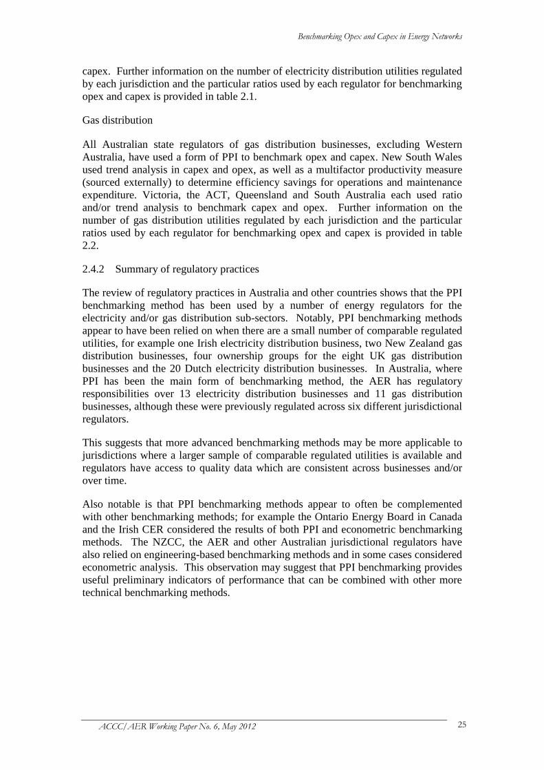
Benchmarking Opex and Capex in Energy Networks
ACCC/AER Working Paper No. 6, May 2012 25
capex. Further information on the number of electricity distribution utilities regulated
by each jurisdiction and the particular ratios used by each regulator for benchmarking
opex and capex is provided in table 2.1.
Gas distribution
All Australian state regulators of gas distribution businesses, excluding Western
Australia, have used a form of PPI to benchmark opex and capex. New South Wales
used trend analysis in capex and opex, as well as a multifactor productivity measure
(sourced externally) to determine efficiency savings for operations and maintenance
expenditure. Victoria, the ACT, Queensland and South Australia each used ratio
and/or trend analysis to benchmark capex and opex. Further information on the
number of gas distribution utilities regulated by each jurisdiction and the particular
ratios used by each regulator for benchmarking opex and capex is provided in table
2.2.
2.4.2 Summary of regulatory practices
The review of regulatory practices in Australia and other countries shows that the PPI
benchmarking method has been used by a number of energy regulators for the
electricity and/or gas distribution sub-sectors. Notably, PPI benchmarking methods
appear to have been relied on when there are a small number of comparable regulated
utilities, for example one Irish electricity distribution business, two New Zealand gas
distribution businesses, four ownership groups for the eight UK gas distribution
businesses and the 20 Dutch electricity distribution businesses. In Australia, where
PPI has been the main form of benchmarking method, the AER has regulatory
responsibilities over 13 electricity distribution businesses and 11 gas distribution
businesses, although these were previously regulated across six different jurisdictional
regulators.
This suggests that more advanced benchmarking methods may be more applicable to
jurisdictions where a larger sample of comparable regulated utilities is available and
regulators have access to quality data which are consistent across businesses and/or
over time.
Also notable is that PPI benchmarking methods appear to often be complemented
with other benchmarking methods; for example the Ontario Energy Board in Canada
and the Irish CER considered the results of both PPI and econometric benchmarking
methods. The NZCC, the AER and other Australian jurisdictional regulators have
also relied on engineering-based benchmarking methods and in some cases considered
econometric analysis. This observation may suggest that PPI benchmarking provides
useful preliminary indicators of performance that can be combined with other more
technical benchmarking methods.
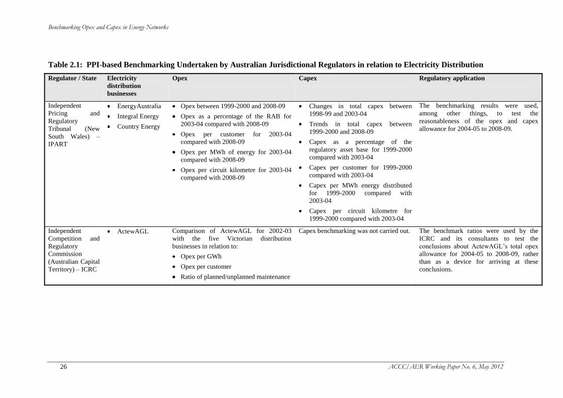
Benchmarking Opex and Capex in Energy Networks
ACCC/AER Working Paper No. 6, May 2012 26
Table 2.1: PPI-based Benchmarking Undertaken by Australian Jurisdictional Regulators in relation to Electricity Distribution
Regulator / State Electricity
distribution
businesses
Opex Capex Regulatory application
Independent
Pricing and
Regulatory
Tribunal (New
South Wales) –
IPART
EnergyAustralia
Integral Energy
Country Energy
Opex between 1999-2000 and 2008-09
Opex as a percentage of the RAB for
2003-04 compared with 2008-09
Opex per customer for 2003-04
compared with 2008-09
Opex per MWh of energy for 2003-04
compared with 2008-09
Opex per circuit kilometre for 2003-04
compared with 2008-09
Changes in total capex between
1998-99 and 2003-04
Trends in total capex between
1999-2000 and 2008-09
Capex as a percentage of the
regulatory asset base for 1999-2000
compared with 2003-04
Capex per customer for 1999-2000
compared with 2003-04
Capex per MWh energy distributed
for 1999-2000 compared with
2003-04
Capex per circuit kilometre for
1999-2000 compared with 2003-04
The benchmarking results were used,
among other things, to test the
reasonableness of the opex and capex
allowance for 2004-05 to 2008-09.
Independent
Competition and
Regulatory
Commission
(Australian Capital
Territory) – ICRC
ActewAGL
Comparison of ActewAGL for 2002-03
with the five Victorian distribution
businesses in relation to:
Opex per GWh
Opex per customer
Ratio of planned/unplanned maintenance
Capex benchmarking was not carried out. The benchmark ratios were used by the
ICRC and its consultants to test the
conclusions about ActewAGL’s total opex
allowance for 2004-05 to 2008-09, rather
than as a device for arriving at these
conclusions.
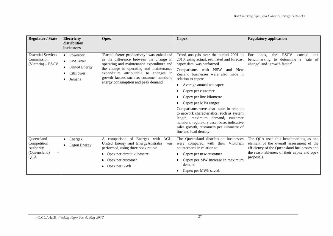
Benchmarking Opex and Capex in Energy Networks
ACCC/AER Working Paper No. 6, May 2012 27
Regulator / State Electricity
distribution
businesses
Opex Capex Regulatory application
Essential Services
Commission
(Victoria) – ESCV
Powercor
SPAusNet
United Energy
CitiPower
Jemena
‘Partial factor productivity’ was calculated
as the difference between the change in
operating and maintenance expenditure and
the change in operating and maintenance
expenditure attributable to changes in
growth factors such as customer numbers,
energy consumption and peak demand.
Trend analysis over the period 2001 to
2010, using actual, estimated and forecast
capex data, was performed.
Comparisons with NSW and New
Zealand businesses were also made in
relation to capex:
Average annual net capex
Capex per customer
Capex per line kilometre
Capex per MVa ranges.
Comparisons were also made in relation
to network characteristics, such as system
length, maximum demand, customer
numbers, regulatory asset base, indicative
sales growth, customers per kilometre of
line and load density.
For opex, the ESCV carried out
benchmarking to determine a ‘rate of
change’ and ‘growth factor’.
Queensland
Competition
Authority
(Queensland) –
QCA
Energex
Ergon Energy
A comparison of Energex with AGL,
United Energy and EnergyAustralia was
performed, using three opex ratios:
Opex per circuit kilometre
Opex per customer
Opex per GWh
The Queensland distribution businesses
were compared with their Victorian
counterparts in relation to:
Capex per new customer
Capex per MW increase in maximum
demand
Capex per MWh saved.
The QCA used this benchmarking as one
element of the overall assessment of the
efficiency of the Queensland businesses and
the reasonableness of their capex and opex
proposals.
Benchmarking Opex and Capex in Energy Networks
ACCC/AER Working Paper No. 6, May 2012 28
Regulator / State Electricity
distribution
businesses
Opex Capex Regulatory application
Essential Services
Commission of
South Australia
(South Australia) –
ESCOSA
ETSA Utilities
Opex benchmarking of ETSA Utilities
against ten other distribution businesses in
relation to:
Opex as a percentage of asset value
Opex per kilometre of line
Opex per customer
Opex per kilovolt ampere (kVa)
maximum demand.
Capex as a percentage of asset value
Capex per kilometre of line
Capex per customer
Capex per kVa maximum demand.
These measures were not used to set opex
or capex, but rather to identify areas where
more detailed analysis may be required.
Office of the
Tasmanian
Economic
Regulator
(Tasmania) –
OTTER
Aurora Energy
The OTTER included in its price
determination trend analysis of Aurora
Energy’s opex over the period 2002-03 to
2011-12.
The OTTER included in its price
determination trend analysis of Aurora
Energy’s capex over the period 2002-03
to 2011-12.
The OTTER considered the use of industry
benchmarking in relation to opex and capex,
and instructed its consultants to consider
high-level comparisons. However, the
OTTER’s consultant did not consider that
weight should be placed on the industry
benchmarking and they were not considered
in the revenue decision.
Economic
Regulation
Authority
(Western
Australia) – ERA
Western Power The efficiency of Western Power’s 2007-08
actual opex relative to other Australian
distribution businesses was assessed by
using benchmarks of the following metrics
prepared by Wilson Cook based on publicly
available information:
Opex per line kilometre
Opex per customer and
Opex per kilowatt hour (kWh).
No capex benchmarking was carried out. The results were only used by the ERA to
assess the base year of 2007-08 and do not
appear to have been used in approving
changes to opex in the access arrangement
for the 2009-10 to 2012-13 period.
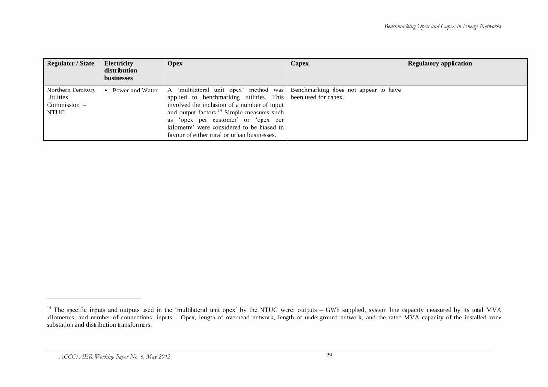
Benchmarking Opex and Capex in Energy Networks
ACCC/AER Working Paper No. 6, May 2012 29
Regulator / State Electricity
distribution
businesses
Opex Capex Regulatory application
Northern Territory
Utilities
Commission –
NTUC
Power and Water A ‘multilateral unit opex’ method was
applied to benchmarking utilities. This
involved the inclusion of a number of input
and output factors.14
Simple measures such
as ‘opex per customer’ or ‘opex per
kilometre’ were considered to be biased in
favour of either rural or urban businesses.
Benchmarking does not appear to have
been used for capex.
14
The specific inputs and outputs used in the ‘multilateral unit opex’ by the NTUC were: outputs – GWh supplied, system line capacity measured by its total MVA
kilometres, and number of connections; inputs – Opex, length of overhead network, length of underground network, and the rated MVA capacity of the installed zone
substation and distribution transformers.
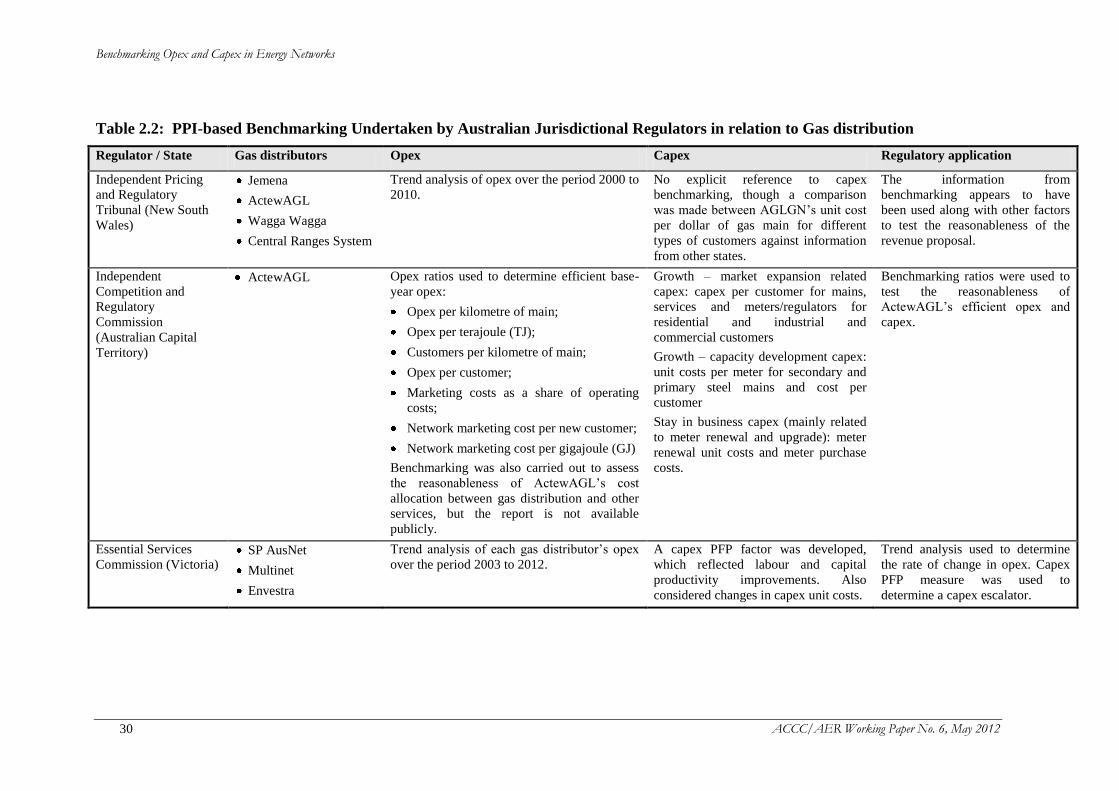
Benchmarking Opex and Capex in Energy Networks
ACCC/AER Working Paper No. 6, May 2012 30
Table 2.2: PPI-based Benchmarking Undertaken by Australian Jurisdictional Regulators in relation to Gas distribution
Regulator / State Gas distributors Opex Capex Regulatory application
Independent Pricing
and Regulatory
Tribunal (New South
Wales)
Jemena
ActewAGL
Wagga Wagga
Central Ranges System
Trend analysis of opex over the period 2000 to
2010.
No explicit reference to capex
benchmarking, though a comparison
was made between AGLGN’s unit cost
per dollar of gas main for different
types of customers against information
from other states.
The information from
benchmarking appears to have
been used along with other factors
to test the reasonableness of the
revenue proposal.
Independent
Competition and
Regulatory
Commission
(Australian Capital
Territory)
ActewAGL Opex ratios used to determine efficient base-
year opex:
Opex per kilometre of main;
Opex per terajoule (TJ);
Customers per kilometre of main;
Opex per customer;
Marketing costs as a share of operating
costs;
Network marketing cost per new customer;
Network marketing cost per gigajoule (GJ)
Benchmarking was also carried out to assess
the reasonableness of ActewAGL’s cost
allocation between gas distribution and other
services, but the report is not available
publicly.
Growth – market expansion related
capex: capex per customer for mains,
services and meters/regulators for
residential and industrial and
commercial customers
Growth – capacity development capex:
unit costs per meter for secondary and
primary steel mains and cost per
customer
Stay in business capex (mainly related
to meter renewal and upgrade): meter
renewal unit costs and meter purchase
costs.
Benchmarking ratios were used to
test the reasonableness of
ActewAGL’s efficient opex and
capex.
Essential Services
Commission (Victoria)
SP AusNet
Multinet
Envestra
Trend analysis of each gas distributor’s opex
over the period 2003 to 2012.
A capex PFP factor was developed,
which reflected labour and capital
productivity improvements. Also
considered changes in capex unit costs.
Trend analysis used to determine
the rate of change in opex. Capex
PFP measure was used to
determine a capex escalator.
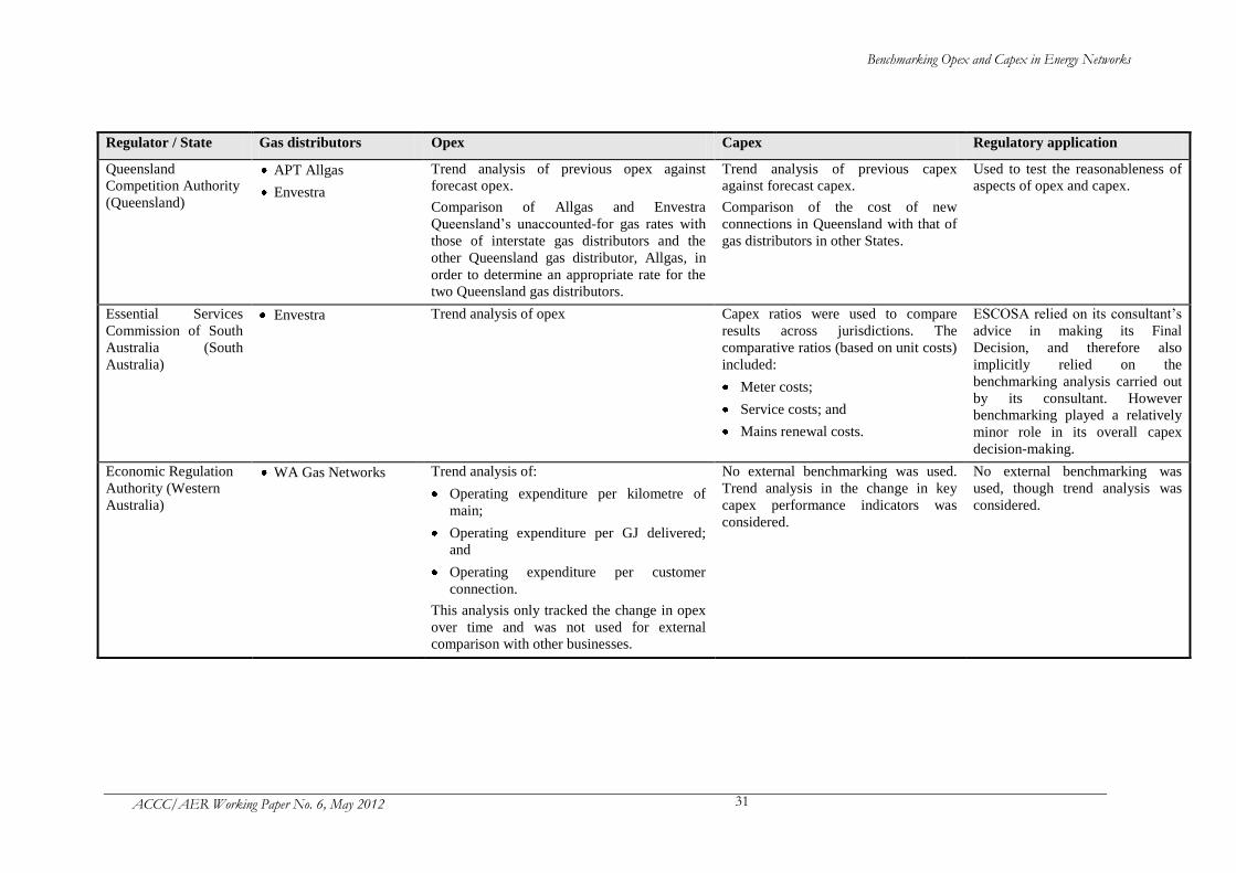
Benchmarking Opex and Capex in Energy Networks
ACCC/AER Working Paper No. 6, May 2012 31
Regulator / State Gas distributors Opex Capex Regulatory application
Queensland
Competition Authority
(Queensland)
APT Allgas
Envestra
Trend analysis of previous opex against
forecast opex.
Comparison of Allgas and Envestra
Queensland’s unaccounted-for gas rates with
those of interstate gas distributors and the
other Queensland gas distributor, Allgas, in
order to determine an appropriate rate for the
two Queensland gas distributors.
Trend analysis of previous capex
against forecast capex.
Comparison of the cost of new
connections in Queensland with that of
gas distributors in other States.
Used to test the reasonableness of
aspects of opex and capex.
Essential Services
Commission of South
Australia (South
Australia)
Envestra Trend analysis of opex Capex ratios were used to compare
results across jurisdictions. The
comparative ratios (based on unit costs)
included:
Meter costs;
Service costs; and
Mains renewal costs.
ESCOSA relied on its consultant’s
advice in making its Final
Decision, and therefore also
implicitly relied on the
benchmarking analysis carried out
by its consultant. However
benchmarking played a relatively
minor role in its overall capex
decision-making.
Economic Regulation
Authority (Western
Australia)
WA Gas Networks Trend analysis of:
Operating expenditure per kilometre of
main;
Operating expenditure per GJ delivered;
and
Operating expenditure per customer
connection.
This analysis only tracked the change in opex
over time and was not used for external
comparison with other businesses.
No external benchmarking was used.
Trend analysis in the change in key
capex performance indicators was
considered.
No external benchmarking was
used, though trend analysis was
considered.
Benchmarking Opex and Capex in Energy Networks
ACCC/AER Working Paper No. 6, May 2012 32
2.5 Issues arising from the review
2.5.1 Limitations of PPI
PPI offers a relatively straightforward method of benchmarking compared with other
benchmarking techniques. However, PPI is of limited use. It considers only one
aspect of a business at a time, namely the business’s inputs and outputs. It does not
account for differences in other aspects of a business. As described earlier, PPI
assumes a linear relationship between inputs and outputs, and that all changes in the
value of an input can be associated with a corresponding change in the output (or vice
versa).
The current literature identifies shortcomings associated with the PPI approach.
These include that PPI only provides a partial indication of performance and cannot
be used to provide an overall ‘benchmark’ performance. CEPA argued that partial
productivity measures can be misleading because they disregard substitution
possibilities between inputs. For example, when capital is substituted for labour in
the production process, labour productivity increases (CEPA, 2003, pp. 25-26).
CEPA noted that the partial approach to productivity measurement neglects the fact
that businesses may choose to substitute one type of expenditure for another, hence
giving them best performance on some measures but not on others, leaving an overall
performance difficult to measure. CEPA (2003) found that compared to PPI, the TFP
approach provides a more complete measure of productivity.
Australian state regulators and the AER have previously found that PPI measurements
were sensitive to the selection of outputs, and that the subsequent results were likely
to be biased in favour of either rural or urban networks (See for example, AER, 2010,
pp. 78-79). That is, using the PPI method, results differ if opex is used as a
proportion of customer numbers, or if opex is used as a proportion of network length.
Consequently, in Australia, while PPI methods have been used to inform the review
process, they have not been used not as a direct input in the determination.
2.5.2 Legislative and regulatory requirements
The National Electricity Rules (NER) govern the operation of the National Electricity
Market and the associated electricity transmission and distribution network service
providers (DNSPs).15
Clauses 6.5.6(e) (regarding opex) and 6.5.7(e) (regarding
capex) of the NER set out the ten factors that the AER must consider when deciding
whether to accept a revenue proposal from an electricity distribution business. Clause
6.5.6(e)(4) specifies that, in assessing a revenue proposal from a DNSP, the AER
must have regard to benchmark operating expenditure that would be incurred by an
efficient DNSP in the given operating circumstances over the regulatory control
period,16
while clause 6.5.7(e)(4) specifies that the AER must have regard to
benchmark capital expenditure.
15
The current consolidated version of the NER is version 49, which can be found at:
http://www.aemc.gov.au/Electricity/National-Electricity-Rules/Current-Rules.html [accessed on 1
March 2012]. 16
Clause 6.5.6(c)(2) of the NER specifies that the AER must accept the forecast of required operating
expenditure of a DNSP if it is satisfied that the total of the forecast operating expenditure for the
regulatory control period reasonably reflects the costs that a prudent operator in the circumstances of
Benchmarking Opex and Capex in Energy Networks
ACCC/AER Working Paper No. 6, May 2012 33
These provisions have been used to support the use of PPI methods as a part of
previous AER reviews.
2.5.3 Industry characteristics
As noted above, the AER must have regard to DNSP-specific business conditions in
the determinations of benchmark operating and capital expenditure. However, a
significant issue in the use of PPI relates to the way in which different operating
environments are treated to allow meaningful comparisons to be made between
different sets of results.
For example, the Irish regulator, in its international benchmarking of opex activities
for electricity distribution found that tree trimming costs per kilometre were lower in
Ireland than in the UK. The UK has higher tree coverage and is subject to stricter
safety regulations. This increases the amount of tree trimming in the UK compared to
Ireland. Costs of fault repairs were also found to be lower in Ireland. This appears to
reflect the fact that the network in Ireland has less underground wires than in the UK.
Underground wires are generally more expensive to repair than overhead wires.
The AER also noted in the Victorian electricity distribution draft determination in
2010 that, differences in network characteristics may impact on the usefulness of
benchmarking.
2.5.4 Data availability and quality
PPI-based benchmarking methods were used in the AER’s Victorian electricity
distribution draft determination in June 2010. The AER identified a number of
limitations with the available data that limited the reliability of the performance
comparisons between distribution businesses in different jurisdictions using PPI
(AER, 2010, pp. 78-79). Specifically, the AER noted the following affect PPI
analysis:
the lumpiness of capex programs;
different licensing requirements between NEM jurisdictions;
differences in whether distribution businesses buy or lease assets;
differences in balance date (i.e., the last day of the company’s financial year);
variations in the characteristics of distribution businesses and the age, size and
maturity of their networks and the markets they serve;
capitalisation, cost allocation and other accounting policies, as well as regulated
service classifications, are assumed to be the same across all DNSPs, and across
regulatory control periods in the sample; and
the nature of the sample of rural, urban and CBD distribution businesses.
the relevant DNSP would require to achieve the operating expenditure objectives. Clause 6.5.7(c)(2)
specifies a similar criteria for accepting capex.
Benchmarking Opex and Capex in Energy Networks
ACCC/AER Working Paper No. 6, May 2012 34
A big challenge to using PPI, and to benchmarking generally, is the comparability of
the data in the AER’s information collection templates (RINs).
Prior to 1 January 2008, state-based regulators oversaw the economic regulation of
DNSPs. In developing RINs for the first round of distribution determinations under
the AER’s jurisdiction, the AER considered potential issues with transitioning from
state based jurisdictional regimes to the national regime. The capex and opex items in
the RINs therefore do not perfectly align between businesses. This has posed
challenges, for example, in the Aurora distribution determinations:
Nuttall Consulting found that sub-transmission lines formed an insignificant part
of Aurora Energy’s (Aurora) capex. In Tasmania, the majority of sub-
transmission assets are owned by a different business, Transend. In contrast,
DNSPs own and operate sub-transmission assets in other jurisdictions.
To improve comparability between Aurora and other DNSPs, Nuttall Consulting
suggested producing ratio analysis charts of all NEM DNSPs using capex data
minus sub-transmission expenditure. However, this was not possible because
data were only available for Aurora and the Victorian DNSPs. That is, only
these Aurora and the Victorian DNSPs separated sub-transmission expenditure
in their RINs.
Nuttall Consulting (2011, pp. 157-160) used ratio analysis charts that compared
Aurora with all other NEM DNSPs. The effect of including sub-transmission
expenditure in the capex ratio analysis is unclear.
Definitions of line items in the capex and opex information between the different
collection templates used by jurisdictional regulators, and subsequently incorporated
into the AER’s RINs, are not identical and thus may not be directly comparable. The
differences result in problems when comparing expenditure between DNSPs. PPI
techniques require consistent ‘like-for-like’ definitions across all businesses in each
subsector. Consistent definitions across jurisdictions also enlarge the sample size
available for analysis. A noteworthy example is the United States, which has long-
standing rules about the public disclosure of detailed financial and operational data on
regulated utilities. The data provided to the Federal Energy Regulatory Commission
(FERC) must comply with the ‘uniform system of accounts’ developed by the
regulator using FERC Form 1 – Electricity Utility Annual Report. The annual reports
from 1994 to 2011 are available from the FERC website.17
In the Aurora distribution determination, Nuttall Consulting performed benchmarking
analysis. Emergency response opex was used in the analysis as this category of opex
was most easily comparable between businesses (Nuttall Consulting, 2011, p. 27).
2.5.5 The use of benchmarking results
Stakeholders and DNSPs often argue that the PPI-based benchmarking used by the
AER is at a very high level, and cannot be used to determine forecast capex or opex.
Indeed, it is difficult to determine an efficient level of capex or opex using this
17
See the FERC website at; http://www.ferc.gov/docs-filling/forms/form-1/data.asp#skipnav [accessed
on 1 March 2012].
Benchmarking Opex and Capex in Energy Networks
ACCC/AER Working Paper No. 6, May 2012 35
approach. For example, is the trend line from a PPI graph (effectively the average of
the scatterplot) indicative of efficient expenditure? Or is further work required to
ascertain the efficient expenditure level?
In response to the 2010 Victorian distribution draft determination, the Energy Users
Association of Australia (EUAA, 2010, p. 20) argued that the benchmarking
techniques used by the AER did not meet minimum standards required by the NER.
The EUAA has urged the AER to develop more extensive benchmarking techniques.
In contrast, EnergyAustralia argued that the differences in benchmarking outcomes
were because of the unique characteristics of each business. EnergyAustralia (2010,
p. 16) argued that because of this, no meaningful conclusions could be drawn from
this level of analysis in relation to the comparative performance of DNSPs.
The debate between stakeholders over the relevance of PPI-based benchmarking
reflects the inherent problems with PPI analysis. These problems suggest a need for
more advanced methods to derive performance measures that can better capture
multiple-input and multiple-output production process (and thus take into account the
potential trade-off between outputs and inputs) and that can adjust for differences in
non-controllable factors affecting utility performance. For example, the Consumer
Action Law Centre (2010, p. 5) recommended developing a TFP approach to limit the
distortions of PPI.
2.6 Conclusions
PPI has been used as an assessment tool in energy regulation in both Australia and a
number of other countries such as Ireland. It has provided regulators with information
on how the performance (e.g., certain expenditure incurred a particular activity) of a
utility compares with others in the industry. The AER has used this as part of its past
assessments to determine where greater scrutiny is required of particular types of
expenditure.
While useful in the regulatory process, PPI has a number of limitations, particularly
relating to data quality and accounting for differing network characteristics and
operating environments. It is also difficult to obtain good price deflators (e.g., for
labour and/or opex) when comparing utilities over time and across geographical
locations. Due to these limitations, PPI-based benchmarking results are best viewed
as providing a useful means of comparison and an indication of where certain
expenditure may be above efficient levels, but should not be viewed in isolation as a
definitive assessment on the efficiency of an energy network business.
Benchmarking Opex and Capex in Energy Networks
ACCC/AER Working Paper No. 6, May 2012 36
Chapter 3 Evaluation of the index-number-based TFP analysis
3.1 Introduction
Total Factor Productivity (TFP) – a ratio of a measure of total output to a measure of
total input use – measures the overall productivity change, which cannot be captured
in a partial performance indicator examining the relationship between one output and
a single factor of production. The TFP method is best used to measure productivity
performance of a business or a group of businesses over time.
There are a number of alternative methods for measuring TFP growth. These include
non-parametric approaches such as index numbers and Data Envelopment Analysis
(DEA), and parametric approaches such as Stochastic Frontier Analysis (SFA) and
econometric cost-function models. Index-number-based TFP is commonly used for
measuring productivity growth when there are a limited number of observations
available. This chapter examines the index-number-based TFP method.
TFP analysis can be used as an informative tool under the current building-block
approach to cross-check the reasonableness of a business’s forecast demand and costs
and thus that of the implied productivity growth potential. For example, under certain
conditions historical productivity growth experienced by comparable utilities in a sub-
sector provides a reasonable benchmark for past and prospect productivity
performance for the utility under consideration. Therefore, a comparison of past
industry-average productivity change with potential growth implied from utility-
specific forecast data can assist the AER’s assessment of expenditure proposals from
individual utilities.
TFP analysis can also be used as a deterministic tool to set revenue or price path,
replacing the building-block approach to assessing expenditure proposals. The
Australian Energy Market Commission (AEMC) has recently completed a review into
the possible uses of a TFP-based method for the determination of prices and revenues
in the national energy markets covering electricity and gas transmission and
distribution sub-sectors.18
The AEMC found that, with more consistent and robust
data, the direct application of an index-number-based TFP method in revenue
determinations could contribute to improvements in electricity and gas network
regulation. In its final decision report, released on 30 June 2011, it was proposing to
the Standing Council on Energy and Resources (SCER, formerly the Ministerial
Council on Energy) initial rules which would facilitate data collection and the
assessment of whether the necessary conditions for introducing TFP as an alternative
to the current building-block approach were met.
The remainder of this chapter is structured as follows: A description of the index-
number-based TFP method is provided in section 3.2. Section 3.3 provides a
summary of academic applications of index-number-based TFP and section 3.4
provides a summary of regulatory applications of the method. Section 3.5 discusses
18
For detailed information, see the AEMC website at: http://www.aemc.gov.au/Market-
Reviews/Completed/Review-Into-the-Use-of-Total-Factor-Productivity-for-the-Determination-of-
Prices-and-Revenues.html [accessed on 3 January 2012].
Benchmarking Opex and Capex in Energy Networks
ACCC/AER Working Paper No. 6, May 2012 37
some of the potential issues associated with the use of index-number-based TFP in
energy regulation and conclusions are drawn in section 3.6
3.2 Description of the TFP method
Total factor productivity (TFP) growth is defined as output growth net of input
growth. There are alternative approaches to the calculation of TFP growth, one of
which is the index-number approach described below.
3.2.1 Method
The index-number approach applies the chosen index number formula to construct
input and output quantity indices. The TFP growth is then defined as the difference
between the rate of output quantity growth and input quantity growth. This approach
is known as ‘growth accounting’; i.e., productivity growth is the residual, or technical
change as defined by Solow (1957), from output growth after accounting for input
growth.
A general form of TFP index (in logarithmic form),19
as defined in Coelli, Rao,
O’Donnell and Battese (2005), is given in the following math equation:
)/()( ststst IndexInputIndexOutputLnTFPLn (3.1)
where the output and input indices are computed using suitable index-number
formulae and subscripts s and t represent two observations (e.g., time periods or
businesses).
The index numbers measure weighted-average change in outputs relative to weighted-
average change in inputs, using revenue and cost shares as the output and input
weights respectively. There are a number of index-number formulae available for
measuring TFP, showing different ways of aggregating inputs and outputs. The
Fisher ideal index (see Fisher, 1922) and the Tornqvist index (see Tornqvist, 1936)
are most frequently used for TFP analysis, owing much to the work of Diewert (1976;
1981; 1992) and Caves, Christensen and Diewert (1982a) that provides the economic
and theoretical justifications for TFP indexes. Box 3.1 provides a mathematical
presentation of Tornqvist index as an example of TFP indexes.
Diewert (1976) showed that a Tornqvist index is a discrete-time approximation for its
continuous-time equivalent Divisia index, implying that the underlying production
function follows a homogenous translog function developed by Christensen,
Jorgenson and Lau (1973). That is, under the assumption of cost minimisation, a
quantity index taking the form of Tornqvist index is consistent with the homogenous
translog function. Diewert (1992) recommended the use of the Fisher ideal index for
TFP work because of its superior axiomatic properties while the Tornqvist index
could also be used as it closely approximates Fisher’s ideal index.
19
The logarithmic form is commonly used due to its computational conveniences and mathematical
properties (i.e., first differentiation is an approximation of growth rate).
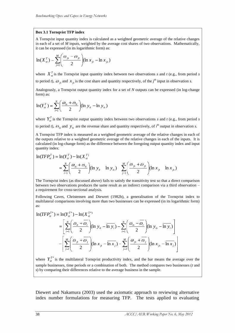
Benchmarking Opex and Capex in Energy Networks
ACCC/AER Working Paper No. 6, May 2012 38
Box 3.1 Tornqvist TFP index
A Tornqvist input quantity index is calculated as a weighted geometric average of the relative changes
in each of a set of M inputs, weighted by the average cost shares of two observations. Mathematically,
it can be expressed (in its logarithmic form) as:
M
j
jsjt
jtjsT
st xxX1
)ln(ln2
)ln(
where T
stX is the Tornqvist input quantity index between two observations s and t (e.g., from period s
to period t), js and jsx is the cost share and quantity respectively, of the jth
input in observation s.
Analogously, a Tornqvist output quantity index for a set of N outputs can be expressed (in log-change
form) as:
N
i
isit
itisT
st yyY1
)ln(ln2
)ln(
where T
stY is the Tornqvist output quantity index between two observations s and t (e.g., from period s
to period t), is and isy are the revenue share and quantity respectively, of ith
output in observation s.
A Tornqvist TFP index is measured as a weighted geometric average of the relative changes in each of
the outputs relative to a weighted geometric average of the relative changes in each of the inputs. It is
calculated (in log-change form) as the difference between the foregoing output quantity index and input
quantity index:
)ln(ln2
)ln(ln2
ln()ln()ln(
11
)
jsjt
M
j
jtjs
isit
N
i
itis
T
st
T
st
T
st
xxyy
XYTFP
The Tornqvist index (as discussed above) fails to satisfy the transitivity test so that a direct comparison
between two observations produces the same result as an indirect comparison via a third observation –
a requirement for cross-sectional analysis.
Following Caves, Christensen and Diewert (1982b), a generalisation of the Tornqvist index to
multilateral comparisons involving more than two businesses can be expressed (in its logarithmic form)
as:
M
j
jjs
jjs
jjt
M
j
jjt
iis
N
i
iis
iit
N
i
iit
T
st
T
st
T
st
xxxx
yyyy
XYTFP
11
11
*)**
)ln(ln2
)ln(ln2
)ln(ln2
)ln(ln2
ln()ln()ln(
where *T
stY is the multilateral Tornqvist productivity index, and the bar means the average over the
sample businesses, time periods or a combination of both. The method compares two businesses (t and
s) by comparing their differences relative to the average business in the sample.
Diewert and Nakamura (2003) used the axiomatic approach to reviewing alternative
index number formulations for measuring TFP. The tests applied to evaluating
Benchmarking Opex and Capex in Energy Networks
ACCC/AER Working Paper No. 6, May 2012 39
quantity indexes included the constant quantities test,20
constant basket test,21
proportional increase in output test,22
and time reversal test.23
Among the four most
popular index formulations evaluated, only the Fisher ideal index satisfies all four
tests. The Laspeyres and Paasche indexes fail the time reversal test,24
while the
Tornqvist index fails the constant basket test. The Fisher index is ‘ideal’ in that it
decomposes the value index exactly into price and quantity components. However,
even the Fisher index fails to satisfy another commonly used test, namely the
circularity (transitivity) test, to ensure that a direct comparison between two
observations produces the same result as an indirect comparison via a third
observation.25
This notwithstanding, transitivity is not considered essential for time-
series analysis, but is required for cross-sectional comparison (Coelli, Rao and
Battese 1998, pp. 91-92).
Conventional TFP indices only measure TFP growth and not TFP levels. Although
they can be used to measure productivity change either over time or across businesses,
it is most commonly used for the former. Transitive multilateral TFP indices,
developed by Caves, Christensen and Diewert (1982b) using the EKS method,26
provide a means of comparing both TFP levels and growth rates using panel data. As
shown in Box 3.1, the essence of these multilateral indices is that comparison between
any pair of two businesses is made relative to the sample-average business to ensure
consistency in the relative productivity levels measured.
Empirical applications of multilateral TFP include Bureau of Industry Economics
(1996) that compared productivity levels and growth rates for electricity supply
businesses in Australia and the United States (US) spanning the period of
corporatisation of the Australian businesses. The study found that the gap between
Australian and US TFP levels narrowed markedly during the corporatisation period.
A series of studies led by Denis Lawrence (see, for example, Lawrence (2003a) and
Lawrence and Diewert (2006)) utilised multilateral TFP to examine comparative
productivity performance for electricity distributors in New Zealand.
3.2.2 Data requirements
The index-number-based TFP method requires price and quantity information on
input and output for two or more businesses or time periods.
20
This states that if quantities are the same in two periods, then the output index should be equal to one
irrespective of the prices of the goods in both periods. 21
This states that if prices are constant over two periods, then the level of output in the current period t
compared to the base period s is equal to the value of output in period t divided by the value of output
in period s. 22
This states that if all outputs in period t are multiplied by a common factor, λ, then the output index
in period t compared to period s should increase by λ. 23
This states that if the prices and quantities in period s and t are interchanged, then the resulting output
index should be the reciprocal of the original index. 24
The Laspeyres index uses the base-period weights whereas the Paasche index uses the current-period
weights to define an index. 25
This states that for any three periods, s, t and b, a direct comparison between periods s and t yields
the same index as an indirect comparison through period b. 26
EKS stands for Elteto-Koves (1964) and Szulc (1964) whose work led to the derivation of transitive
index numbers for multilateral price comparison.
Benchmarking Opex and Capex in Energy Networks
ACCC/AER Working Paper No. 6, May 2012 40
The essential pieces of information include price and quantity of each input variable
and each output variable to model. While quantity information on output (e.g.,
number of customers or kilowatt hours of electricity sold) is generally available,
information on the physical quantity of inputs (e.g., labour, capital, and other inputs)
may not be readily available. For example, for labour input, the measure of number
of full-time-equivalent (FTE) staff or total hours worked may not be reported to the
regulator or published in the public domain. Indirect measures that deflate value of
the relevant costs (e.g., labour costs) by suitable price indexes (e.g., labour price
index) may be used to obtain implicit quantity measures. The price indexes used may
not be perfect because they are generally compiled for the industry by a statistical
agency (for details, see Coelli, Estache, Perelman and Trujillo, 2003, p. 29).
Of the inputs modelled, capital input is most problematic to measure, which may
explain the common practice of benchmarking opex as opposed to the ‘total cost’
approach. The calculation of capital input in terms of physical quantity (and cost) is
important for TFP analysis, particularly in a capital-intensive network industry. The
proper measure of capital input is the flow of capital services during a period. A
proxy is the measure of capital stock in place, which is assumed to be in proportion to
the periodic flow of capital services, regardless of the age of assets. For electricity
distribution, physical quantities of two main distribution assets are commonly
modelled – network line length (in route/circuit kilometres) and installed transformer
capacity (in megavolt amperes – MVa).27
This specification implies the one-hoss
shay model of physical deterioration that assumes constant provision of services at
full productive efficiency until the end of the service life of an asset.28
Other
depreciation profiles may also be assumed in the empirical studies; for example, a
declining-balance approach to depreciation called perpetual inventory method (PIM)
has generally been adopted in the consultancy work conducted by Pacific Economics
Group (PEG) for constructing the constant-dollar replacement cost of utility assets
using detailed capital data over time.
For TFP analysis, price or revenue/cost share information is also required as weights
to aggregate relevant inputs and outputs. Where revenue/cost shares for outputs
modelled are not directly observable, either empirical evidence is required (e.g.,
estimating econometric cost functions) or a subjective judgement needs to be made on
the appropriate weights to attribute to the outputs specified. As noted above, the input
price indexes may be sourced from statistical agencies. A service-price approach to
capital cost measurement is generally used to measure the price of periodical capital
services, which incorporates three components reflecting depreciation rate (the return
of capital), opportunity cost (the return on capital) and capital gains. Alternatively,
the cost of using capital inputs may be measured indirectly at ex post return (i.e., the
residual between revenue and operating costs realised) if restrictive assumptions about
the technology and market characteristics are held to be true.29
27
Network line length models transmission of energy to customer, and installed transformer capacity
captures transformation of high voltage energy to low-voltage energy. 28
A number of researchers in the area consider that the one-hoss shay depreciation pattern reasonably
reflects the depreciation process in electricity distribution. See for example, Makholm and Quinn
(2003, p. 5) and Lawrence and Diewert (2006, p. 217). For a definition of the term, see OECD (2012). 29
These include competitive input and output markets and constant returns-to-scale production
technology. See relevant discussions in Hulten (1986).
Benchmarking Opex and Capex in Energy Networks
ACCC/AER Working Paper No. 6, May 2012 41
Additional information on key operating environmental characteristics may also be
required for the TFP analysis. The relevant data can be used for testing whether the
businesses should be grouped on the basis of comparable operating environments or
for second-stage regression analysis to adjust business performance for external
factors that are beyond management control.30
For electricity distribution businesses,
key operating environment conditions that may affect productivity performance
include (but are not limited to):
energy density as measured by GWh per circuit kilometre;
customer density, measured as customers per square km of service area or
customers per route kilometre;
network density, measured as route kilometre per square kilometre of service
area;
peak demand: note that this may also be included as an output in the model
specification;
customer mix, measured as the ratio of domestic customers to commercial and
industrial customers; and
the ratio of underground to overhead network.
The datasets used can be cross-sectional data that compare productivity differences
across businesses at a point in time, time-series data that examine productivity change
of the business (industry, sector or economy) over time, or panel data for both time-
series and cross-sectional productivity analysis. For possible regulatory applications,
the availability of a quality and reliable TFP dataset that covers comparable
businesses over a sufficiently long time period is desirable.
3.2.3 Advantages and disadvantages
The index-number-based TFP can be used to measure productivity change either over
time or across businesses. It is most commonly used for time-series analysis to
measure temporal TFP change and/or gauge trend TFP growth.
The index-number-based TFP has a number of merits. First, the commonly adopted
Tornqvist or Fisher TFP indexes have economic-theoretic properties relating to the
underlying production technology that they present. Second, all inputs can be
accounted for conceptually. Third, it requires fewer observations than alternative
approaches to measuring productivity change (e.g., Malmquist TFP index under DEA
or SFA). Fourth, the approach is relatively simple and transparent, and the results are
readily reproducible.
However, the index-number-based TFP approach is associated with certain
limitations. The approach can be information-intensive as it requires not only
30
For example, an input-requirements function can be estimated econometrically to adjust total input
usage for a range of operating environment factors. This will then permit the calculation of the input
usage that would be required by each distributor if they all faced the same values of the specified
operating environment variables.
Benchmarking Opex and Capex in Energy Networks
ACCC/AER Working Paper No. 6, May 2012 42
quantity information, but also price (or revenue/cost share) information to compute
the TFP index. As a non-parametric technique, it cannot produce confidence intervals
and other statistical tests. Further, unlike TFP measured under DEA or SFA, index-
number-based TFP does not allow for a decomposition of productivity changes into
the sources. Implicitly assumed under growth accounting are full technical
efficiency,31
constant returns to scale (CRS), a behavioural objective such as cost
minimisation, and neutral technical progress. If these assumptions are inconsistent
with the data, then the index number method will provide a biased estimate of
technical change that can be attributable to a combination of factors, such as changes
in technical efficiency, allocative efficiency or scale efficiency.
3.3 Literature review of the TFP method
3.3.1 Literature review
The index-number-based TFP method has been used in several studies on all or part
of the energy sector in Australia, covering a broad range of research objectives. An
early study conducted by Lawrence, Swan and Zeitsch (1991) used multilateral TFP
to examine the productivity of Australian state-based vertically integrated electricity
authorities. The study found great variations in productivity changes across states, but
the differences declined over time. Later studies were carried out to examine the
impact of microeconomic reform on the energy sector. In assessing the productivity
performance of the electricity supply sub-sector in New South Wales (NSW), Pierce,
Price and Rose (1995) reviewed a number of empirical studies, including two studies
(London Economics and Energy Supply Association of Australia (ESAA); 1993,
1994) of New South Wales metropolitan distributors supplying distribution and
retailing services, commissioned by the Independent Pricing and Regulatory Tribunal
of New South Wales (IPART). The review found that productivity improvements
were realised by each distributor over the sample period 1981-82 to 1993-94.
Jamasb and Pollitt (2001) discussed the use of index-number-based TFP as a
benchmarking technique for regulatory purposes. They noted that the method could
use the Tornqvist index as a measure of historical productivity growth at the firm,
industry, or economy-level and in setting the productivity-offsetting factor X in price-
cap regulation. In their view, this method is relatively easy to implement, but may
inadvertently favour less efficient firms, as they may be in a better position than more
efficient firms to outperform the uniform productivity target and earn large profits.32
The IPART commissioned a report on the efficiency of NSW electricity distribution
businesses (i.e., London Economics, 1999) that benchmarked the NSW utilities
against 219 utilities operating in Australia, New Zealand, the US and the UK, using
DEA. Various other benchmarking techniques were used for sensitivity analysis of
31
The work of Balk (1998) relaxed the assumption of full technical efficiency in deriving various index
numbers. 32
By their nature, less efficient businesses are theoretically more capable of making productivity gains
than more efficient businesses, as they are more capable of implementing changes to their businesses
that will improve efficiency and lead to greater productivity (assuming that all businesses face the same
environment).
Benchmarking Opex and Capex in Energy Networks
ACCC/AER Working Paper No. 6, May 2012 43
the DEA results, including Tornqvist TFP.33
The Tornqvist TFP index was calculated
for the NSW distributors using a single output – total energy delivered (GWh), three
inputs – total operating and maintenance (O&M) expenditure (in 1997-98 $AUS),
route kilometres and nameplate transformer capacity, and cost share information from
other similar Australian electricity distributors as the input weights. The outcome of
the review indicated inefficiency among the NSW electricity distribution businesses.
Cambridge Economics Policy Associates (CEPA 2003) prepared a report for the
Ofgem to develop the use of benchmarking in the 2005 electricity distribution price
control review (DPCR4). The report reviewed the Ofgem’s past practices;34
alternative benchmarking methods; the appropriateness of cost drivers; and
distribution network service data in 2001-02 for an application of the COLS method
used in DPCR3. CEPA (2003) considered a combination of DEA and COLS as the
most appropriate approach to determining the efficiency frontier for the distributors,
given the data currently available. CEPA (2003) considered that the index-number-
based TFP method was useful for assessing frontier shift, but, found that, due to the
disparity shown in the estimated productivity performance, there were application
issues for setting the firm-specific X factors.
CEPA (2003) also raised an issue with examining opex efficiency alone. The TFP
results showed that businesses that displayed limited improvements in opex
performance, despite being some way from the frontier, had generally shown good
improvements in TFP under the totex approach. Nevertheless, measuring the capital
expenditure element of totex is not straightforward.35
Lawrence (2005a), in a commissioned report, examined the performance of Western
Power’s distribution operations over the period 1999 to 2003 compared to 12 other
Australian electricity distribution businesses. A comprehensive range of performance
indicators was used for comparative performance analysis. The TFP analysis
specified three outputs – energy throughput in gigawatt-hours, system capacity in
MVa-kilometres and number of customers, and five inputs – O&M expenditure,
overhead lines, underground lines, transformers, and other capital. According to the
report, this three-output specification has the advantage of incorporating key features
of the main density variables (customers per kilometre and sales per customer) driving
distributors’ costs. The report considered that the comprehensive analysis enabled
effective benchmarking of the many facets of electricity distributor performance.
Lawrence and Diewert (2006) conducted a TFP study that was used by the New
Zealand Commerce Commission (NZCC) as the basis for setting X factors under the
CPI–X regulation for electricity networks in New Zealand. Price-path thresholds
were in place which set a maximum change in real output prices that each distribution
network business would be allowed without triggering further investigation. The X
factors in the thresholds were made up of three components: a B factor reflecting
33
Additional analyses included: sensitivity analysis using SFA, sensitivity checks (such as those based
on exchange rates) and a second-stage Tobit regression to adjust the DEA efficiency scores to account
for environmental differences. 34
The Ofgem previously used Corrected Ordinary Least Squares (COLS) regression to benchmark
distribution businesses on normalised controllable operating costs. 35
This issue is discussed further in chapter 8 of this paper.
Benchmarking Opex and Capex in Energy Networks
ACCC/AER Working Paper No. 6, May 2012 44
industry-wide TFP growth, a C1 factor reflecting comparative-productivity
performance and a C2 factor reflecting comparative profitability.
Using multilateral TFP and econometric cost function methods, TFP levels and
growth rates for 29 electricity distributors were examined over an eight-year period
from 1996 to 2003. With three outputs – energy throughput in gigawatt–hours,
system capacity in MVa-kilometres, and number of customers; and five inputs –
O&M expenditure, overhead lines, underground lines, transformers, and other capital
a Fisher TFP index was calculated. As revenue for each output specified was
unobservable, the study used the relative shares of cost elasticities derived from an
econometric cost function estimated for the sampled New Zealand distributors.
In this study, Lawrence and Diewert (2006, p. 215) provided reasons for not including
a quality variable (e.g., frequency and duration of interruptions). They considered
that the index-number-based TFP does not incorporate ‘bad outputs’ (i.e., a decrease
in the measure represents an increase in service-quality output) easily. They also
discussed other major measurement problems encountered in electricity network
productivity studies, particularly the specification of outputs and capital inputs. This
work (commissioned by the Commerce Commission) has been published in various
forms: see for example, Lawrence, Diewert and Kain (2007), and Lawrence (2003a).
Makholm and Quinn (2003) provided a detailed description of the index-number-
based TFP method and its potential use in the price-cap regulation for electricity
distribution; applying the method to the determination of the productivity of
electricity distribution networks in the United States. A Tornqvist TFP index was
constructed with principal outputs, measured according to customer groups (by either
number of customers, system capacity or sales volume) – residential, commercial,
industrial or public entities, and three categories of inputs – labour, capital, and
material and others. Relevant regulatory data on 87 companies operating in 37 states
over 23 years from 1972 to 1994 were used to measure TFP at the industry level and
for each of the four regions (i.e., northeast, midwest, south and west). The authors
suggested using the estimated industry-wide TFP growth as a productivity-offsetting
factor (X factor) in the price-cap formula. The authors considered the TFP method a
useful tool for computing the X factor under the price-cap regulatory formulas.
In a study commissioned by the AEMC, Brattle Group (2008) reviewed the use of
TFP in energy network regulation outside Australia. International experience using
TFP includes electricity distribution in New Zealand; gas distribution in Ontario,
Canada; energy networks in the UK; electricity distribution in the Netherlands; and
selected jurisdictions in North America. The report first examined how each regulator
had gone about the process of undertaking a TFP study; and second, how TFP results
were used in determining the maximum allowed growth rate of regulated prices. The
report also discussed design issues associated with TFP measurement and practice,
one of which is the time period for measuring TFP growth. Brattle Group (2008, p. 4)
considered that using the longest time period possible to compute average TFP growth
over the longer term could mitigate the impact of cyclical variations, temporary and
one-off events.
Another study by Economic Insights (2009a) was also commissioned by the AEMC to
conduct a sensitivity analysis of TFP results to variations in the estimation method,
including alternative output and input specifications, lengths of the time period, and
Benchmarking Opex and Capex in Energy Networks
ACCC/AER Working Paper No. 6, May 2012 45
methods used for indexing, weighting inputs and outputs, and calculating the TFP
growth rates. The study found that (Economic Insights, 2009a, pp. i-v, 22-23):
sensitivity of input-output specifications depends on whether the alternative
outputs (and inputs) grow at similar or different rates;
the difference in results from the use of the Fisher and Tornqvist indexes may
not be material; and
the difference in using the average methods as opposed to the use of regression-
based methods for calculating growth rates can be substantial. This is
demonstrated by the application to estimating TFP growth for the Victorian gas
distribution sub-sector between 1998 and 2007. The geometric-average growth
rate was found to be substantially different from the trend growth rate when the
starting and ending years were outlying observations relative to the trend of the
intervening years.
3.3.2 Summary of the studies
The literature review shows that a number of empirical studies have applied the
index-number-based TFP method to the examination of the energy sector in Australia
and other countries. Table 3.1 below summarises the studies specific to electricity
distribution networks in terms of methods (including index-number-based TFP), index
formula (Tornqvist versus Fisher index), data, input-out specification and other
important elements of the TFP analysis.
In summary, the literature suggests that the Fisher index and the Tornqvist index are
commonly used for TFP analysis, and that time-series or panel data are generally used
to measure industry-level productivity growth. The choice of input-output
specifications is often constrained by data availability and quality. For example,
single or multiple output measures may be used due to the availability of the relevant
revenue/cost share information. The capital input raises some measurement issues.
There is also some debate on the appropriate output quantity measures. It does not
appear to be a common practice to use second-stage regression analysis to test the
significance of a range of operating environmental factors in explaining the
differences in productivity change.
In general, there is a consensus that the index-number-based TFP method is a useful
tool for calculating the productivity-offsetting factor under the CPI–X price-cap
regulatory formulas. However, depending on the regulatory framework, the method
may not necessarily be used as the primary assessment tool. Instead, it can be used
for sensitivity analysis to check the robustness of results with respect to method.

Benchmarking Opex and Capex in Energy Networks
ACCC/AER Working Paper No. 6, May 2012 46
Table 3.1: Summary of the Literature Applying TFP to Benchmarking Energy Networks*
Author/s Country /
Territory
Sector / years Methods Inputs Outputs Other factors/specification
issues/findings
London
Economics (1999)
NSW
(Australia), New
Zealand, the UK
and the US
6 electricity
distribution
businesses in NSW
(1995-96 to 1997-98)
DEA – VRS (primary);
SFA; TFP (Tornqvist) Total O&M expenditure
(1997-98 $AUS)
Route kilometres36
Nameplate transformer capacity
Total energy delivered
(GWh)
Tornqvist TFP index was
computed for NSW distributors as
part of the sensitivity analysis.
Makholm and
Quinn (2003)
US Electricity
distribution (1972 to
1994)
TFP (Tornqvist) Labour
Capital (one-hoss shay)
Material and other operating
costs
Outputs by customer type
(residential, commercial,
industrial and public
entities)
The paper suggested using the
estimated industry-wide TFP
growth as the productivity-
offsetting factor in the price-cap
formula.
CEPA (2003) UK Electricity
distribution (1997-98
to 2001-02)
COLS, SFA, DEA, TFP
(Tornqvist), Partial
factor productivity
(PFP)
Total expenditure
Total energy delivered
(GWh)
Total number of
customers
Network length
Wide disparities in the firm-level
performance showed that it was
premature to use these directly to
set X factors. However, TFP can
be a useful tool for assessing
frontier shift.
Lawrence (2005a) Australia Electricity
distribution (1999 to
2003)
TFP, PPI Total O&M expenditure
(constant price)
Overhead lines
Underground line
Transformer capacity
Other capital
Total energy delivered
(GWh)
Total number of
customers
System capacity (MVa)
The report considered that
comprehensive performance
analysis enabled effective
benchmarking of electricity
distribution businesses.
Lawrence and
Diewert (2006)
New Zealand 29 electricity
distribution
businesses (1996 to
2003)
TFP Total O&M expenditure
Overhead lines
Underground line
Transformer capacity
Other capital
Total energy delivered
(GWh)
Total number of
customers
System capacity (MVa)
An econometric cost function was
estimated to inform the cost share
of outputs specified.
* The ‘Inputs’ and ‘Outputs’ columns of the table only present the input-output specifications for the index-number-based TFP analysis.
36
The route kilometres measure is the linear distance between poles regardless of how many circuits are supported. The circuit kilometres measure is the length between
poles by number of circuits, which is at least the same as route kilometres. Countries/jurisdictions may report one or both of the measures. For example, route kilometre
measure is available for the US distributors while the UK and NZ distributors report only circuit kilometres (London Economics, 1999, p. 38).
Benchmarking Opex and Capex in Energy Networks
ACCC/AER Working Paper No. 6, May 2012 47
3.4 Regulatory practices using the TFP method
3.4.1 Regulatory practices review
Index-number-based TFP benchmarking methods have been used by energy
regulators in the determination of price and revenue requirements for electricity and
gas distribution businesses in countries, such as Australia, New Zealand, the
Netherlands, Germany, and Austria, and in some Canadian provinces (e.g., Ontario).
In addition, state-based regulators in the US, such as the California Public Utilities
Commission (CPUC), have received applications from energy utilities that include
supporting productivity studies on the basis of index-number-based TFP and
econometric cost function methods.37
Germany and Austria38
According to WIK-Consult (2011), the regulation of electricity and gas distribution
sub-sectors in Germany and Austria has involved the use of index-number-based TFP
analysis to estimate the frontier shift component of the X factor. The X factor also
incorporates a business-specific efficiency improvement component (or stretch factor)
which has been determined using alternative benchmarking methods such as DEA and
Modified Ordinary Least Squares (refer to sections 6.4 and 4.4 respectively).
The energy regulator in Austria, E-control, decided on a frontier shift at 1.95 per cent
per annum for both electricity and gas distribution based on its review of international
studies, international practices, own preliminary calculation and consultation with
stakeholders (WIK-Consult, 2011, p. 7). The Federal Network Agency (BNetzA) in
Germany applied the Tornqvist TFP index to the computation of the frontier shift
component, the value of which was heavily disputed. Several industry-commissioned
studies suggested lower values, based on different data sources and base periods. The
High Court decision finally ruled out the inclusion of industry-economy productivity
differential in the revenue-cap formula (WIK-Consult, 2011, pp. 29-31).
However, for these two countries, no detailed information on the derivation of the
frontier shift component is available from the relevant regulatory decision papers.
The determination of this component is often a result of a bargaining process between
stakeholders rather than a regulatory decision based on sound and transparent
economic analysis (WIK-Consult, 2011, p. 60).
California, United States39
In many US states, performance-based regulation (PBR) has been adopted for the
regulation of electricity and gas distribution businesses. TFP studies, sometimes
combined with the econometric cost model approach, have been submitted by the
regulated utility as supporting evidence and thus have become an important input to
the regulatory process of setting of the X factor. The TFP studies typically examine
37
As it is not possible to cover all countries, there may be other examples of energy regulators applying
TFP benchmarking methods that have not been captured in this paper and the supporting research.
Haney and Pollitt (2009) undertook a survey of current benchmarking methods applied by energy
regulators worldwide. 38
Refer to sections 3.1 and 3.4 of WIK-Consult (2011). 39
Refer to chapter seven of ‘Regulatory Practices in Other Countries’ (ACCC/AER, 2012).
Benchmarking Opex and Capex in Energy Networks
ACCC/AER Working Paper No. 6, May 2012 48
industry and company-specific TFP performance using the index-number approach
(Division of Ratepayer Advocates (DRA), 2007, p. 1).
For example, in California, price caps in the form of industry-specific inflation index
and productivity index differential (including a stretch factor) were approved by the
CPUC for the gas and electricity distribution services of San Diego Gas and Electric
Company (SDG&E) in 1999 for the years 1999 to 2002 and subsequently extended to
2003 (Lowry and Getachew 2009c, p. 67). As part of this process SDG&E
commissioned PEG to conduct an index-number-based TFP analysis for both its
electricity distribution and gas distribution services (PEG, 2008, p. 97). Similar
supporting TFP studies have since been presented to the CPUC by SDG&E in
subsequent General Rate Case (GRC) applications in 2003, 2008 and 2011.40
SDG&E has also commissioned efficiency benchmarking studies using the
econometric cost function method to support its argument for a zero value of the
stretch factor in the GRC application in 2008.41
The final regulatory decisions were
based on a settlement process between SDG&E and DRA (and other stakeholders).
For SDG&E’s 2008 GRC, the supporting PEG study used Tornqvist TFP index to
estimate productivity trends for the sampled US utilities as a group, large Californian
utilities as a group, and SDG&E itself. Gas distribution and electricity distribution
were estimated separately. The weights used to construct weighted-average output
growth were derived from the econometric cost model approach.
Details of the electricity distribution analysis are:
Sample: a total of 77 major investor-owned electricity distributors in the US
over the period 1994 to 2004;
Services covered: electricity distributor services covering distribution, customer
accounts, sales and general administration;
Outputs: electricity sales (in kilowatt hours; 50 per cent) and customers (50 per
cent);42
and
Inputs: cost weighted sum of labour, capital, fuel and non-labour O&M inputs.
Details of the gas distribution analysis are:
Sample: 34 large gas distributors, from 1994 to 2004. Some gas distributors also
provided gas transmission and/or storage services;
Services covered: gas distributor services covering costs comprising O&M
expenses and costs of plant ownership applicable to distributing gas. Expenses
for customer service and information and uncollectible bills were excluded
40
A General Rate Case (GRC) occurs when the utility requests that the regulator considers future
tariffs proposal. GRCs generally occur every three to four years. 41
The description is not based on the original PEG study, primarily drafted by Mark Lowry, due to no
access to the report. Instead, the summary is based on two papers – Lowry and Getachew (2009c) that
summarised the PEG indexing and benchmarking work and Division of Ratepayer Advocates (DRA)
(2007) that replicated and critiqued that PEG study. 42
The output weights were taken from the cost elasticity results in the accompanying econometric cost
modelling of electricity distribution undertaken in the original PEG study.
Benchmarking Opex and Capex in Energy Networks
ACCC/AER Working Paper No. 6, May 2012 49
because those expenses rose sharply over the sample period due to circumstances
beyond management control;
Outputs: throughput (27 per cent) and customers (73 per cent);43
and
Inputs: cost weighted sum of labour, capital, fuel and non-labour O&M inputs.
Ontario, Canada44
Electricity distribution
In Canada, PEG studies have been used in informing the Ontario Energy Board
(OEB)’s determination of the price path for electricity distribution businesses. Since
2000, the OEB has introduced an incentive regulation framework based on a price cap
of the form: PCI = P − X ± Z where the growth in the price cap index (PCI) is
determined by the inflation rate (P), a productivity-offsetting factor (X) and an
additional factor to account for unforseen events (Z).
The X factor includes an industry-wide productivity component estimated by the
index-number-based TFP method, an inflation differential component and a ‘stretch
factor’ estimated by the unit-cost and econometric methods (refer to sections 2.4 and
4.4 respectively).
The estimate of industry-wide productivity was based on a long-run TFP trend
analysis conducted by PEG using US data for the period 1988 to 2006 as a proxy for
the Ontario electricity distribution sub-sector. The US data were used as the Ontario
data were not sufficiently long to estimate a long-run productivity growth. The study
is similar to the TFP analysis performed for the study of SDG&E (PEG, 2008, p. 34),
including the following:
Tornqvist index;
TFP trend is the simple average of annual TFP growth rates;
Three inputs (capital, labour, and materials and services) and two outputs
(number of retail customers and total electricity deliveries – kWh); and
Econometric model was used to determine cost elasticity shares to weigh
outputs (PEG, 2008, pp. 128-132).
Gas distribution
TFP analysis has also been undertaken by PEG and the Brattle Group for Canada’s
gas distribution industry. The PEG study, commissioned by the OEB, used an
econometric approach to estimate TFP. The Brattle Group study, commissioned by
Enbridge (one of the two major distributors in Ontario), used an index-number-based
approach to estimate TFP. In both studies, the X factor was calculated as the sum of a
‘productivity differential’ component and an ‘input price differential’ component.
The productivity differential was the difference between the productivity trends of the
43
The output weights were taken from the cost elasticity results in the accompanying econometric cost
modelling of gas distribution undertaken in the original PEG study. 44
Refer to chapter six of ‘Regulatory Practices in Other Countries’ (ACCC/AER, 2012).

Benchmarking Opex and Capex in Energy Networks
ACCC/AER Working Paper No. 6, May 2012 50
gas distribution industry and the economy as a whole. The input price differential
was calculated as difference between the input price trends in the economy as a whole
and the gas sub-sector in particular.
As with electricity distribution, estimation of the historic TFP growth was undertaken
using data from 36 US gas distributors as a proxy for the Canadian gas distribution
sub-sector. In the index-number-based TFP application, the Brattle Group study
specified four inputs (labour, material and supply, capital, and gas use) and volume of
gas distributed, disaggregated by customer type, as output measures.
However, the results from these TFP studies were not used directly by the OEB in its
final determination. Rather, the OEB determined revenues by the application of a
‘distribution revenue requirement per customer’ formula.
New Zealand45
As discussed above in section 3.3, the index-number-based TFP method has been
used in New Zealand for setting the X factor(s) under the CPI–X price path for
electricity distribution and gas pipeline businesses.46
For this purpose, the New
Zealand Commerce Commission commissioned a number of productivity studies, led
by Lawrence (some reviewed in section 3.3 above), to measure industry-wide
productivity growth.
Electricity distribution
In a series of studies performed by Lawrence (see for example, Lawrence 2003a and
Economic Insights 2009b), the index-number-based TFP method was employed for
determining industry-wide productivity for the regulatory periods 2004 to 2009 and
2010 to 2015 respectively. For the period 2004 to 2009 under the previous threshold
regulatory regime, the X factor included the estimates of industry-wide productivity
relative to economy-wide productivity and an input price differential, comparative
productivity and comparative profitability. For the period 2010 to 2015, the X factor
consisted of only the estimate of industry-wide productivity relative to economy-wide
productivity and the input price differential.
The data used for measuring industry-wide TFP covered 28 electricity distributors
since 1996. The Fisher index was used to measure productivity of the electricity
distribution sub-sector using three outputs – energy throughput in gigawatt–hours,
system capacity in MVa–kilometres and number of customers, and five inputs –
O&M expenditure, overhead lines, underground lines, transformers, and other capital.
The output weights were based on the cost elasticity results derived from an
econometric cost function study by Lawrence (2003a).
In addition, under the previous threshold regulatory regime which applied from 2001
to 2009, multilateral TFP analysis was also undertaken to determine the comparative
productivity component. The results were used to group electricity distributors and
assign stretch factors. The amendments to the Commerce Act in 2008 prohibit the
45
Refer to chapter four of ‘Regulatory Practices in Other Countries’ (ACCC/AER, 2012). 46
Electricity distribution and gas pipeline (transmission and distribution) businesses are subject to
default price–quality path regulation, where the price path is of a CPI–X form. The electricity and gas
default price-quality paths are assessed separately.

Benchmarking Opex and Capex in Energy Networks
ACCC/AER Working Paper No. 6, May 2012 51
inclusion of comparative performance in the setting of the new default price-quality
paths.
Gas distribution
Lawrence, through Economic Insights, was also engaged by the Commerce
Commission to assess whether, for New Zealand, long–run productivity growth rates,
as well as input price growth, were significantly different between gas pipeline
businesses (i.e., distribution and transmission pipelines) and the economy as a whole.
With data only available for the three gas pipeline businesses between 2006 and 2010,
a preliminary TFP analysis was undertaken based on two inputs, opex and pipeline
length, and two outputs, energy throughput and customer numbers. Different input
and output weightings were considered and compared. The analysis was
‘exploratory’ in the sense that additional data would have been required to estimate a
long-run average industry productivity growth rate. Economic Insights (2011) also
examined the literature for TFP results for overseas gas distribution businesses and for
other New Zealand industries. The results assisted the Commerce Commission in
setting a zero X factor in the default price-quality path applying to all New Zealand
gas pipeline businesses.
Australia
In Australia where the forward-looking, multi-year building-block-model (BBM)
framework has been commonly adopted, ratio and trend analysis have been the most
commonly used benchmarking approaches although TFP, PFP, multifactor
productivity and regression analysis have had limited application. It is noted that:
In assessing Power and Water Corporation’s electricity distribution services, the
Northern Territory Utilities Commission (NTUC) used TFP to determine the X
factor in the CPI–X price path formula for the 2009-10 to 2013-14 regulatory
period with the base-year costs determined using a building-block-model
approach (NTUC, 2009); and
Jemena Gas Networks in NSW, Envestra Queensland and Envestra South
Australia all presented the AER with TFP analysis as part of their recent gas
access arrangement reviews. The analysis also included Partial Factor
Productivity (PFP) analysis.
GHD Meyrick was engaged by the NTUC to advise on the TFP application. To that
effect, GHD Meyrick reviewed relevant academic and regulatory evidence, providing
productivity growth trends in electricity distribution industries in New Zealand, the
US and Victoria. GHD Meyrick also performed a TFP analysis of Power and Water
Power Networks (PWPN) covering the years 2000 to 2008 (GHD Meyrick, 2008).
The chained Fisher index was used to measure TFP for electricity distribution
modelled by three outputs (throughput – gigawatt-hour, system line capacity – MVa
kilometres, and number of connections) and four inputs (opex – constant price,
overhead network, underground network, and transformers). The output weights
used were based on Lawrence (2003a), which produced ‘an output cost share for
throughput of 22 per cent, for system line capacity of 32 per cent and for connections
of 46 per cent’ (GHD Meyrick, 2008, p. 13). The results were used by the NTUC
(2009, p. 43) to decide the long-run industry TFP growth.
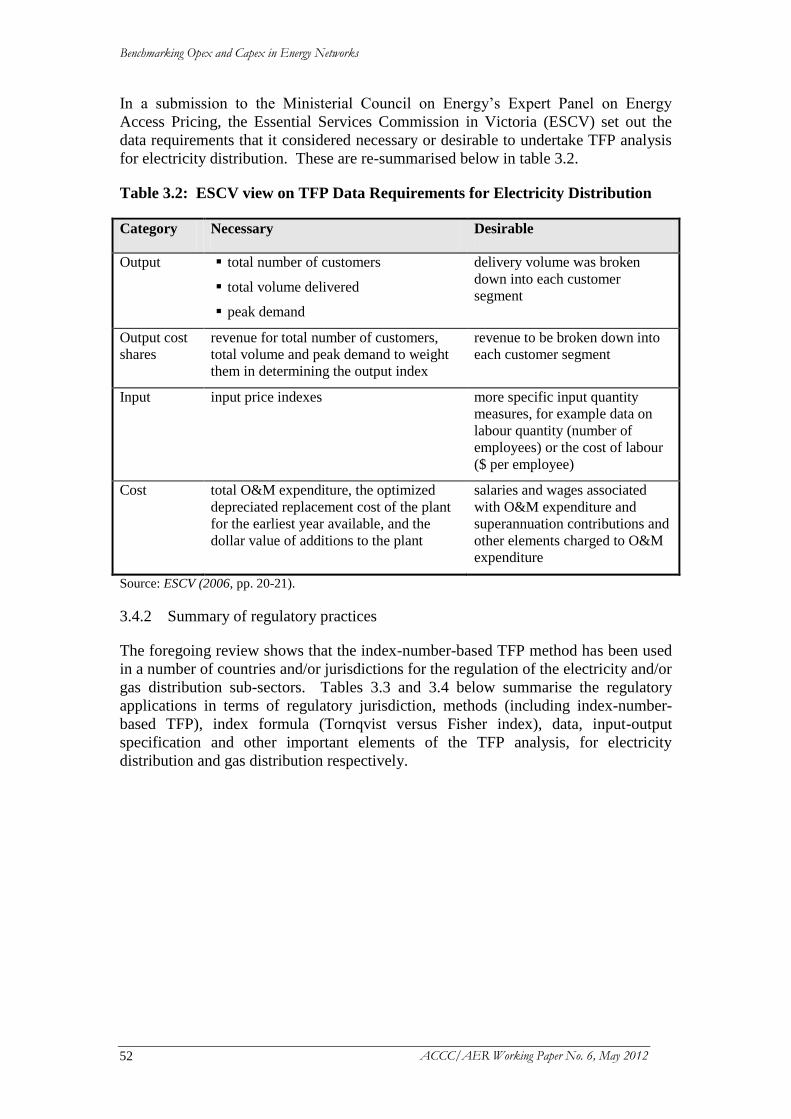
Benchmarking Opex and Capex in Energy Networks
ACCC/AER Working Paper No. 6, May 2012 52
In a submission to the Ministerial Council on Energy’s Expert Panel on Energy
Access Pricing, the Essential Services Commission in Victoria (ESCV) set out the
data requirements that it considered necessary or desirable to undertake TFP analysis
for electricity distribution. These are re-summarised below in table 3.2.
Table 3.2: ESCV view on TFP Data Requirements for Electricity Distribution
Category Necessary Desirable
Output total number of customers
total volume delivered
peak demand
delivery volume was broken
down into each customer
segment
Output cost
shares
revenue for total number of customers,
total volume and peak demand to weight
them in determining the output index
revenue to be broken down into
each customer segment
Input input price indexes more specific input quantity
measures, for example data on
labour quantity (number of
employees) or the cost of labour
($ per employee)
Cost total O&M expenditure, the optimized
depreciated replacement cost of the plant
for the earliest year available, and the
dollar value of additions to the plant
salaries and wages associated
with O&M expenditure and
superannuation contributions and
other elements charged to O&M
expenditure
Source: ESCV (2006, pp. 20-21).
3.4.2 Summary of regulatory practices
The foregoing review shows that the index-number-based TFP method has been used
in a number of countries and/or jurisdictions for the regulation of the electricity and/or
gas distribution sub-sectors. Tables 3.3 and 3.4 below summarise the regulatory
applications in terms of regulatory jurisdiction, methods (including index-number-
based TFP), index formula (Tornqvist versus Fisher index), data, input-output
specification and other important elements of the TFP analysis, for electricity
distribution and gas distribution respectively.
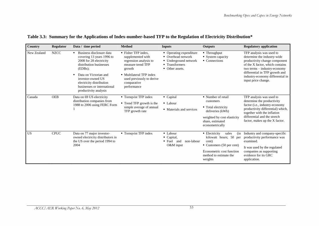
Benchmarking Opex and Capex in Energy Networks
ACCC/AER Working Paper No. 6, May 2012 53
Table 3.3: Summary for the Applications of Index-number-based TFP to the Regulation of Electricity Distribution*
Country Regulator Data / time period Method Inputs Outputs Regulatory application
New Zealand NZCC Business disclosure data
covering 13 years 1996 to
2008 for 28 electricity
distribution businesses
(EDBs);
Data on Victorian and
investor-owned US
electricity distribution
businesses or international
productivity analysis
Fisher TFP index,
supplemented with
regression analysis to
measure trend TFP
growth
Multilateral TFP index
used previously to derive
comparative
performance
Operating expenditure
Overhead network
Underground network
Transformers
Other assets.
Throughput
System capacity
Connections
TFP analysis was used to
determine the industry-wide
productivity change component
of the X factor, which contains
two terms – industry-economy
differential in TFP growth and
industry-economy differential in
input price change.
Canada OEB Data on 69 US electricity
distribution companies from
1988 to 2006 using FERC Form
1
Tornqvist TFP index
Trend TFP growth is the
simple average of annual
TFP growth rate
Capital
Labour
Materials and services
Number of retail
customers
Total electricity
deliveries (kWh)
weighted by cost elasticity
share, estimated
econometrically
TFP analysis was used to
determine the productivity
factor (i.e., industry-economy
productivity differential) which,
together with the inflation
differential and the stretch
factor, makes up the X factor.
US CPUC Data on 77 major investor-
owned electricity distributors in
the US over the period 1994 to
2004
Tornqvist TFP index Labour
Capital,
Fuel and non-labour
O&M input
Electricity sales (in
kilowatt hours; 50 per
cent)
Customers (50 per cent)
Econometric cost function
method to estimate the
weights
Industry and company-specific
productivity performance was
examined.
It was used by the regulated
companies as supporting
evidence for its GRC
application.
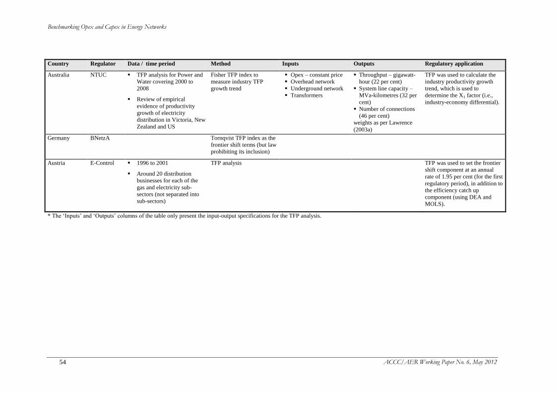
Benchmarking Opex and Capex in Energy Networks
ACCC/AER Working Paper No. 6, May 2012 54
Country Regulator Data / time period Method Inputs Outputs Regulatory application
Australia NTUC TFP analysis for Power and
Water covering 2000 to
2008
Review of empirical
evidence of productivity
growth of electricity
distribution in Victoria, New
Zealand and US
Fisher TFP index to
measure industry TFP
growth trend
Opex – constant price
Overhead network
Underground network
Transformers
Throughput – gigawatt-
hour (22 per cent)
System line capacity –
MVa-kilometres (32 per
cent)
Number of connections
(46 per cent)
weights as per Lawrence
(2003a)
TFP was used to calculate the
industry productivity growth
trend, which is used to
determine the X1 factor (i.e.,
industry-economy differential).
Germany BNetzA Tornqvist TFP index as the
frontier shift terms (but law
prohibiting its inclusion)
Austria E-Control 1996 to 2001
Around 20 distribution
businesses for each of the
gas and electricity sub-
sectors (not separated into
sub-sectors)
TFP analysis TFP was used to set the frontier
shift component at an annual
rate of 1.95 per cent (for the first
regulatory period), in addition to
the efficiency catch up
component (using DEA and
MOLS).
* The ‘Inputs’ and ‘Outputs’ columns of the table only present the input-output specifications for the TFP analysis.
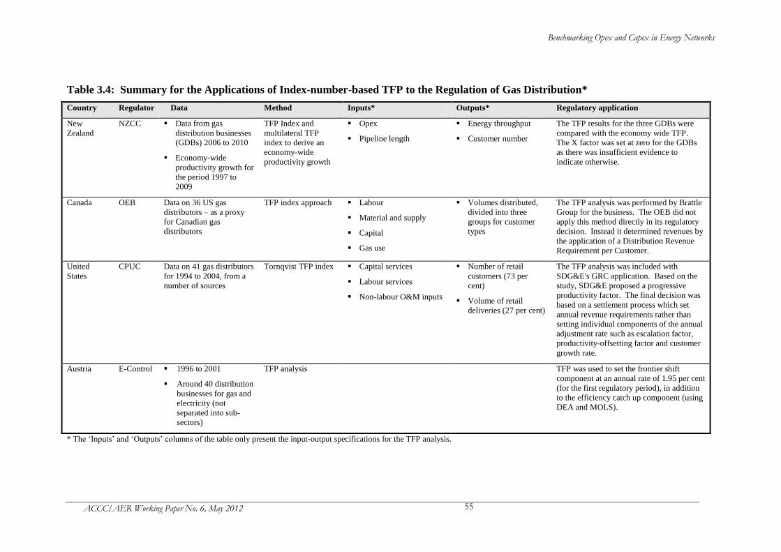
Benchmarking Opex and Capex in Energy Networks
ACCC/AER Working Paper No. 6, May 2012 55
Table 3.4: Summary for the Applications of Index-number-based TFP to the Regulation of Gas Distribution*
Country Regulator Data Method Inputs* Outputs* Regulatory application
New
Zealand
NZCC Data from gas
distribution businesses
(GDBs) 2006 to 2010
Economy-wide
productivity growth for
the period 1997 to
2009
TFP Index and
multilateral TFP
index to derive an
economy-wide
productivity growth
Opex
Pipeline length
Energy throughput
Customer number
The TFP results for the three GDBs were
compared with the economy wide TFP.
The X factor was set at zero for the GDBs
as there was insufficient evidence to
indicate otherwise.
Canada OEB Data on 36 US gas
distributors – as a proxy
for Canadian gas
distributors
TFP index approach Labour
Material and supply
Capital
Gas use
Volumes distributed,
divided into three
groups for customer
types
The TFP analysis was performed by Brattle
Group for the business. The OEB did not
apply this method directly in its regulatory
decision. Instead it determined revenues by
the application of a Distribution Revenue
Requirement per Customer.
United
States
CPUC Data on 41 gas distributors
for 1994 to 2004, from a
number of sources
Tornqvist TFP index Capital services
Labour services
Non-labour O&M inputs
Number of retail
customers (73 per
cent)
Volume of retail
deliveries (27 per cent)
The TFP analysis was included with
SDG&E's GRC application. Based on the
study, SDG&E proposed a progressive
productivity factor. The final decision was
based on a settlement process which set
annual revenue requirements rather than
setting individual components of the annual
adjustment rate such as escalation factor,
productivity-offsetting factor and customer
growth rate.
Austria E-Control 1996 to 2001
Around 40 distribution
businesses for gas and
electricity (not
separated into sub-
sectors)
TFP analysis TFP was used to set the frontier shift
component at an annual rate of 1.95 per cent
(for the first regulatory period), in addition
to the efficiency catch up component (using
DEA and MOLS).
* The ‘Inputs’ and ‘Outputs’ columns of the table only present the input-output specifications for the TFP analysis.
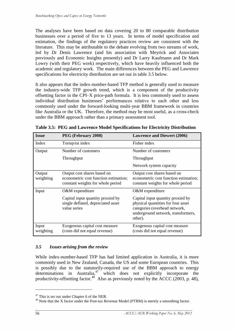
Benchmarking Opex and Capex in Energy Networks
ACCC/AER Working Paper No. 6, May 2012 56
The analyses have been based on data covering 20 to 80 comparable distribution
businesses over a period of five to 13 years. In terms of model specification and
estimation, the findings of the regulatory practices review are consistent with the
literature. This may be attributable to the debate evolving from two streams of work,
led by Dr Denis Lawrence (and his association with Meyrick and Associates
previously and Economic Insights presently) and Dr Larry Kaufmann and Dr Mark
Lowry (with their PEG work) respectively, which have heavily influenced both the
academic and regulatory work. The main differences between the PEG and Lawrence
specifications for electricity distribution are set out in table 3.5 below.
It also appears that the index-number-based TFP method is generally used to measure
the industry-wide TFP growth trend, which is a component of the productivity
offsetting factor in the CPI–X price-path formula. It is less commonly used to assess
individual distribution businesses’ performances relative to each other and less
commonly used under the forward-looking multi-year BBM framework in countries
like Australia or the UK. Therefore, the method may be most useful, as a cross-check
under the BBM approach rather than a primary assessment tool.
Table 3.5: PEG and Lawrence Model Specifications for Electricity Distribution
Issue PEG (February 2008) Lawrence and Diewert (2006)
Index Tornqvist index Fisher index
Output Number of customers
Throughput
Number of customers
Throughput
Network system capacity
Output
weighting
Output cost shares based on
econometric cost function estimation;
constant weights for whole period
Output cost shares based on
econometric cost function estimation;
constant weights for whole period
Input O&M expenditure
Capital input quantity proxied by
single deflated, depreciated asset
value series
O&M expenditure
Capital input quantity proxied by
physical quantities for four asset
categories (overhead network,
underground network, transformers,
other).
Input
weighting
Exogenous capital cost measure
(costs did not equal revenue)
Exogenous capital cost measure
(costs did not equal revenue)
3.5 Issues arising from the review
While index-number-based TFP has had limited application in Australia, it is more
commonly used in New Zealand, Canada, the US and some European countries. This
is possibly due to the statutorily-required use of the BBM approach to energy
determinations in Australia,47
which does not explicitly incorporate the
productivity-offsetting factor.48
Also as previously noted by the ACCC (2003, p. 48),
47
This is set out under Chapter 6 of the NER. 48
Note that the X factor under the Post-tax Revenue Model (PTRM) is merely a smoothing factor.
Benchmarking Opex and Capex in Energy Networks
ACCC/AER Working Paper No. 6, May 2012 57
index-number-based TFP and other benchmarking approaches are difficult to
undertake because of the limited productivity data available and the potential for
variations in productivity growth between individual businesses. More recently, in
the review of the TFP approach to regulation, the AEMC found that one of the
reasons for limited use of benchmarking techniques in the AER’s regulatory
determinations was because of a lack of consistent data needed to apply
benchmarking techniques (AEMC, 2011, p. ii). Indeed, the AEMC recommended the
establishment of a more robust and consistent dataset facilitating the use of TFP
indexes (AEMC, 2011, p. ii). Australian researchers in the field of productivity and
efficiency analysis have long and constantly argued for this (see, for example, Coelli,
Estache, Perelman and Trujillo, 2003; Lawrence, 2003b; and Economic Insights,
2009c). In the US, the Federal Energy Regulatory Commission (FERC) has
assembled a comprehensive historical database that is suitable for productivity
analysis.
Nevertheless, the National Electricity Law (NEL) and National Gas Law (NGL)
permit rules to allow the use of index-number-based TFP, either as a deterministic or
informative tool, in addition to the existing building-block approach (AEMC, 2009,
p. ix). It is therefore important to understand the issues that may arise when using an
index-number-based TFP method for regulatory purposes.
3.5.1 Data requirements
The index-number-based TFP method requires price and quantity information on
inputs and outputs for comparable businesses over a sufficiently long time period so
that the long-run industry productivity growth trend can be accurately estimated for
informing the appropriate productivity-saving target.
Under the AEMC review, a set of pre-conditions for the possible application of TFP
to the Australian energy networks is identified (AEMC, 2009, p. 47). The first
condition is the availability of robust and credible data. In addition, the TFP
measurement must: accurately reflect the industry’s productivity growth; be
immutable to the behaviour of the regulated businesses and regulator; represent
comparable businesses; and reflect stable business performance. Finally, historical
TFP performance must be a good indication for future productivity growth; that is, it
must be a good predictor.
According to the AEMC, it is likely that a TFP application could be appropriate for
use in the electricity and gas distribution sub-sectors; however, an improvement in
regulatory reporting requirements is needed first (AEMC, 2009, p. 79). This implies
that, for the electricity distribution sub-sector, although the industry characteristics are
suitable for ‘forming a stable, comparable industry-wide benchmark’ (Brattle Group,
2008, p. 8), it may take a few more years to get the required data to accurately
measure the long-run industry productivity growth.
As pointed out by Economic Insights (2009c, p. 18), without a high degree of data
consistency and comparability, TFP analysis may not be suitable for being a
deterministic tool for setting revenues/prices. Its assessment of the available data
showed that the key requirement for a consistent set of TFP data – detailed and
consistent definitions of key input, output and environmental condition variables to be
reported – was not met.
Benchmarking Opex and Capex in Energy Networks
ACCC/AER Working Paper No. 6, May 2012 58
Data availability and quality is a key precondition for the regulatory use of TFP
analysis. In general, the more disaggregated the specifications in relation to
heterogeneous inputs and outputs, the more accurate the measure of aggregate output
growth and input growth, and thus TFP growth. However, the choice of input and
output specifications is often constrained by the availability of quality data. Data
availability and quality may also limit what data adjustment or normalisation can be
performed to ensure like-with-like comparisons across businesses.
3.5.2 Model specifications
The following issues in relation to model-specification and measurement of variables
regularly arise in the literature:
Output specification and measurement:
o The output specifications for the many dimensions of an energy network
service typically cover the demand-side of services. That is, the output
specifications generally include measures of electricity delivered and
customers connected. However, they do not always address the supply-
side of network provision. That is, they may not include coverage and the
capacity of the network and the quality and reliability of supply (e.g.,
frequency and duration of outages).
o Demand-side models tend to favour urban distributors with dense
networks. Supply-side models tend to favour rural distributors with sparse
networks and long line lengths. Some studies, for example those by
Lawrence (e.g., Lawrence and Diewert, 2006) suggest that it is important
to account for both supply and demand sides of services in the TFP
analysis, and to consider the impact of different operating conditions.
However CEPA (2003, p. 88) argues that it is risky to include network
length as an output variable (or account for network density) as this may
introduce perverse incentives for the businesses because it may encourage
network expansion only to improve measures of relative efficiency
performance.
o Consistent data measuring any of the three aspects of quality of services –
reliability of supply (e.g., System average interruption duration index
(SAIDI), System average interruption frequency index (SAIFI), Customer
average interruption duration index (CAIDI), Momentary average
interruption frequency index (MAIFI)), technical quality of services (e.g.,
number of complaints, distribution network loss or cost of loss), and
quality of customer services (e.g., call centre performance) – are generally
not available.
o Additional reasons for the failure to incorporate quality of services in the
index-number-based TFP analysis are: first, the method does not easily
incorporate ‘bad outputs’ (i.e., a decrease in the measure represents an
increase in service-quality output); and second, it is difficult to value

Benchmarking Opex and Capex in Energy Networks
ACCC/AER Working Paper No. 6, May 2012 59
quality improvement to consumers in order to weigh the quality output
appropriately.49
Input specification and measurement: labour, materials and services, and capital
are inputs that are generally modelled in productivity studies. Capital input is
more difficult to measure consistently. This is discussed in section 3.2.
Output weighting: prices for the multi-dimension outputs are generally not
directly observable. Where revenue/cost share information for outputs is not
available, empirical evidence may be used, such as econometric studies that
estimate the relevant cost functions. In the alternative, a subjective judgement
may need to be made to determine the weights to attribute different outputs.
Input weighting: capital input price may be measured directly. For example,
data may be used in relation to the annual user cost of capital, taking account of
depreciation, opportunity costs and capital gains. Alternatively, capital input
price may be measured indirectly through the realised residual between total
revenue and operating and maintenance costs. The direct or indirect measure of
capital input price may generate differences in the calculated rates of TFP. The
AEMC considered that capital user costs should be set exogenously for
consistency with regulatory asset base (RAB) and the ex ante financial capital
maintenance (FCM) (AEMC, 2011, p. 24).
In relation to alternative model specifications, it is important to consider the
assumptions underpinning the model and their implications for the TFP measurement.
If there is no strong theoretical foundation favouring a particular model specification,
sensitivity analysis can be conducted to ensure robustness of the results.
Finally, while differences in operating conditions are likely to affect achievable unit
costs and productivity levels, their impact on business-specific productivity growth
remains an empirical question (AEMC, 2010, p. 77). The literature suggests that, in
energy distribution studies, energy density and customer density are generally found
to be the two significant operating environment variables affecting unit costs and
productivity levels. See for example, AEMC (2008, s. 3.1.1, p. 2) and Lawrence,
Diewert and Kain (2007, p. 10). With limited and inconclusive evidence on their
productivity growth impact, it is important to empirically examine the impact of key
operating conditions in a study of energy networks. It may be necessary to group
businesses based on comparable operating environments in order to generate robust TFP
results that are appropriate for regulatory use.
3.5.3 Applications
Index-number-based TFP can be used to measure historical long-run industry
productivity growth. The estimate can then be used as the best proxy for future
productivity growth to determine the productivity-offsetting factor in the CPI–X
price-path formula. This approach has had limited application in Australia under the
BBM framework.
49
Recent studies on French electricity distribution by Coelli, Crespo, Paszukiewicz, Perelman, Plagnet
and Romano (2008) and Coelli, Gautier, Perelman and Saplacan-Pop (2010) have estimated shadow
prices for quality of services using Data Envelopment Analysis and Stochastic Frontier Analysis.
Benchmarking Opex and Capex in Energy Networks
ACCC/AER Working Paper No. 6, May 2012 60
While index-number-based TFP can be an important tool for estimating past
productivity growth patterns, regulatory purposes require an assessment of future
growth. Clearly, there is a need to consider whether past trends will reasonably be
expected to reflect future growth. That is, the regulatory question is forward-looking,
to examine the extent to which the regulated companies could be reasonably expected
to reduce future costs, in real terms. Therefore, it is important to consider whether
future productivity growth prospects are likely to depart from the historical long-run
industry performance.
3.6 Conclusions
The review into the literature and regulatory practices shows that the benchmark
industry-wide productivity growth rate derived from the index-number-based TFP
method can be used either to inform or determine the productivity-offsetting factor –
an implicit or explicit component to consider for setting revenues or prices for energy
network service providers. The effective use of index-number-based TFP method in
energy regulation requires fundamentally ‘reliable, credible historical data reported
regularly and consistently’ (Utility Regulators Forum, 2005, p. 6) and an accurate
measure of the underlying long-run productivity growth.
Benchmarking Opex and Capex in Energy Networks
ACCC/AER Working Paper No. 6, May 2012 61
Chapter 4 Evaluation of the econometric approach to benchmarking
4.1 Introduction
A central task of any utility regulator is the determination of a level of revenue which
is sufficient for a business, operating under a given incentive framework and
operating environment, to cover the costs of delivering a given set of outputs. In
order to carry out this task, the regulator must form a view about the cost structure
underlying the industry. This assessment may be captured by the use of a ‘cost
function’, which shows the output-cost relationship for a cost-minimising business.
That is, by modelling the technology in place, the output quantities, the input prices,
and the operating conditions in which the business operates, a minimum-cost function
yields the periodic costs incurred by an efficient business to deliver those services in
that environment.
Therefore, the econometric modelling of the cost function requires information on: the
cost incurred, the range of services that the businesses produce (in quantity), the
prices for inputs, and the operating environmental conditions. It also requires the
selection of the functional form to use. Conventionally, least-squares-type estimation
or other appropriate estimation methods are used to econometrically estimate the
parameters of the cost function for comparable businesses in an industry. For
benchmarking purposes, the estimated results are then used to derive the expenditures
required by individual businesses if they are minimising costs (the ‘benchmark cost’),
which are to be compared with their observed costs. Any difference in the observed
cost from the benchmark cost is attributable exclusively or largely to management-
controllable inefficiency. One of the shortcomings of the conventional econometric
approach to benchmarking is that it does not allow for a separate random error term
from the inefficiency term in the modelling. This is addressed by the more advanced
Stochastic Frontier Analysis (SFA), as further explored in Chapter 5.
A number of academic studies and utility regulators have pursued this approach for
modelling the energy networks, particularly for those operating in electricity and gas
distribution.
The remainder of this chapter is structured in five parts. The next section describes
this econometric approach to benchmarking in more detail. Section 4.3 briefly
reviews the literature on the econometric approach to benchmarking energy networks.
Section 4.4 reviews the practices of energy regulators which have applied the
econometric method. Section 4.5 identifies the potential issues associated with the
use of the econometric approach to benchmarking, and section 4.6 concludes.
4.2 Description of the econometric approach to benchmarking
4.2.1 Method
The econometric approach to benchmarking estimates a common benchmark cost
function for a set of businesses.
Given a vector of outputs , a vector of input prices
, and a vector of environmental variables , a
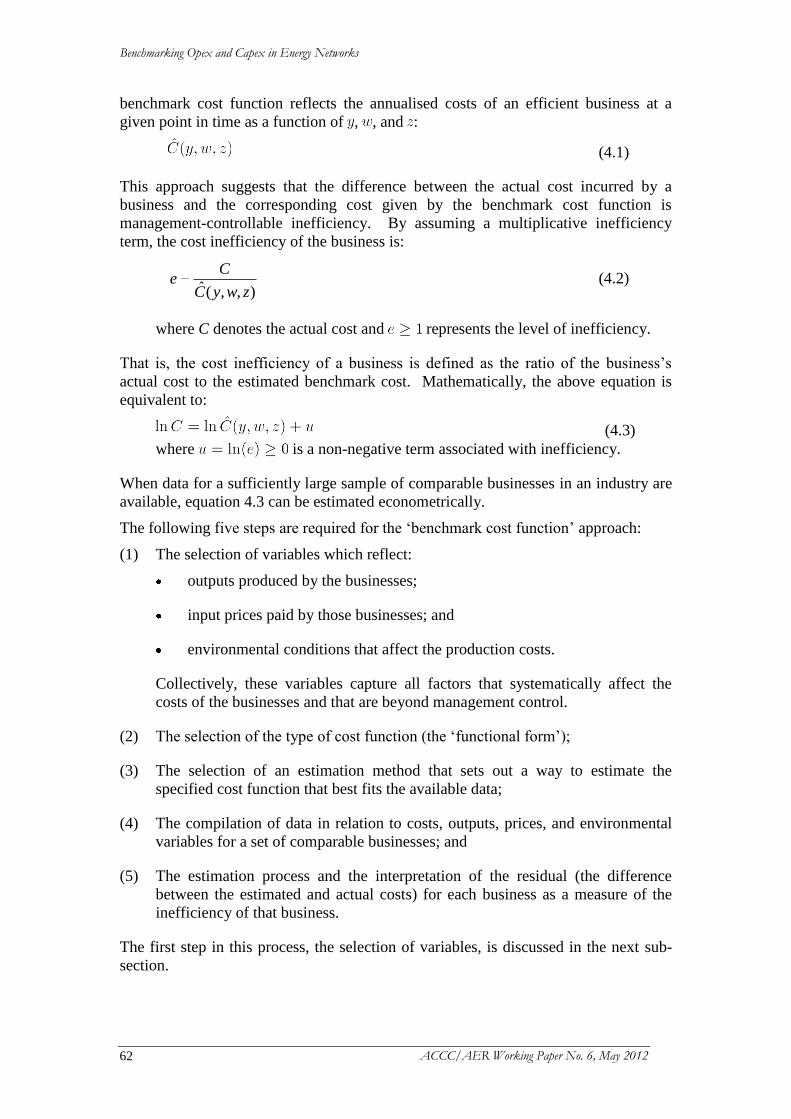
Benchmarking Opex and Capex in Energy Networks
ACCC/AER Working Paper No. 6, May 2012 62
benchmark cost function reflects the annualised costs of an efficient business at a
given point in time as a function of , , and :
(4.1)
This approach suggests that the difference between the actual cost incurred by a
business and the corresponding cost given by the benchmark cost function is
management-controllable inefficiency. By assuming a multiplicative inefficiency
term, the cost inefficiency of the business is:
),,(ˆ zwyC
Ce (4.2)
where C denotes the actual cost and represents the level of inefficiency.
That is, the cost inefficiency of a business is defined as the ratio of the business’s
actual cost to the estimated benchmark cost. Mathematically, the above equation is
equivalent to:
(4.3)
where is a non-negative term associated with inefficiency.
When data for a sufficiently large sample of comparable businesses in an industry are
available, equation 4.3 can be estimated econometrically.
The following five steps are required for the ‘benchmark cost function’ approach:
(1) The selection of variables which reflect:
outputs produced by the businesses;
input prices paid by those businesses; and
environmental conditions that affect the production costs.
Collectively, these variables capture all factors that systematically affect the
costs of the businesses and that are beyond management control.
(2) The selection of the type of cost function (the ‘functional form’);
(3) The selection of an estimation method that sets out a way to estimate the
specified cost function that best fits the available data;
(4) The compilation of data in relation to costs, outputs, prices, and environmental
variables for a set of comparable businesses; and
(5) The estimation process and the interpretation of the residual (the difference
between the estimated and actual costs) for each business as a measure of the
inefficiency of that business.
The first step in this process, the selection of variables, is discussed in the next sub-
section.
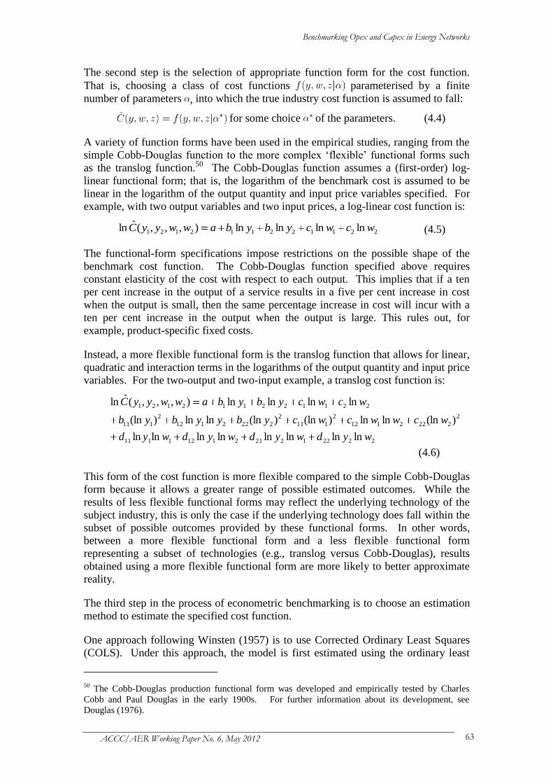
Benchmarking Opex and Capex in Energy Networks
ACCC/AER Working Paper No. 6, May 2012 63
The second step is the selection of appropriate function form for the cost function.
That is, choosing a class of cost functions parameterised by a finite
number of parameters , into which the true industry cost function is assumed to fall:
for some choice of the parameters. (4.4)
A variety of function forms have been used in the empirical studies, ranging from the
simple Cobb-Douglas function to the more complex ‘flexible’ functional forms such
as the translog function.50
The Cobb-Douglas function assumes a (first-order) log-
linear functional form; that is, the logarithm of the benchmark cost is assumed to be
linear in the logarithm of the output quantity and input price variables specified. For
example, with two output variables and two input prices, a log-linear cost function is:
221122112121 lnlnlnln),,,(ˆln wcwcybybawwyyC (4.5)
The functional-form specifications impose restrictions on the possible shape of the
benchmark cost function. The Cobb-Douglas function specified above requires
constant elasticity of the cost with respect to each output. This implies that if a ten
per cent increase in the output of a service results in a five per cent increase in cost
when the output is small, then the same percentage increase in cost will incur with a
ten per cent increase in the output when the output is large. This rules out, for
example, product-specific fixed costs.
Instead, a more flexible functional form is the translog function that allows for linear,
quadratic and interaction terms in the logarithms of the output quantity and input price
variables. For the two-output and two-input example, a translog cost function is:
2222122121121111
2
2222112
2
111
2
2222112
2
111
221122112121
lnlnlnlnlnlnlnln
)(lnlnln)(ln)(lnlnln)(ln
lnlnlnln),,,(ˆln
wydwydwydwyd
wcwwcwcybyybyb
wcwcybybawwyyC
(4.6)
This form of the cost function is more flexible compared to the simple Cobb-Douglas
form because it allows a greater range of possible estimated outcomes. While the
results of less flexible functional forms may reflect the underlying technology of the
subject industry, this is only the case if the underlying technology does fall within the
subset of possible outcomes provided by these functional forms. In other words,
between a more flexible functional form and a less flexible functional form
representing a subset of technologies (e.g., translog versus Cobb-Douglas), results
obtained using a more flexible functional form are more likely to better approximate
reality.
The third step in the process of econometric benchmarking is to choose an estimation
method to estimate the specified cost function.
One approach following Winsten (1957) is to use Corrected Ordinary Least Squares
(COLS). Under this approach, the model is first estimated using the ordinary least
50
The Cobb-Douglas production functional form was developed and empirically tested by Charles
Cobb and Paul Douglas in the early 1900s. For further information about its development, see
Douglas (1976).
Benchmarking Opex and Capex in Energy Networks
ACCC/AER Working Paper No. 6, May 2012 64
squares (OLS) regression. This is followed by a second step where the intercept
parameter a is shifted down by the smallest estimated residual (i.e., the most negative
residual). This correction is to ensure that the estimated frontier bounds the data
points from below. Given certain stringent conditions, COLS provides consistent and
unbiased estimates of the parameters of the selected cost function. Under the COLS
approach, the business with the smallest estimated residual is assumed to be efficient
and thus operate on the estimated cost frontier. Other businesses are relatively
inefficient, the extent of which is the difference between their residuals and that of the
identified efficient business.
A variation on COLS is the modified ordinary least squares approach (MOLS), as
proposed by Afriat (1972) and Richmond (1974). Similar to COLS, the cost function
is initially estimated using OLS. The estimated intercept is then shifted down by the
mean of an assumed one-sided distribution of cost inefficiencies. The distributions
assumed include an exponential or half normal distribution. A more recent
application is proposed by Lowry, Getachew and Hovde (2005), which measured the
cost inefficiency ‘relative to the average rather than the frontier’ (p. 81) using a
maximum-likelihood estimation (MLE)-equivalent generalised least squares (GLS)
method suitable for an unknown structure of the error distribution.
While these econometric techniques are relatively straightforward, they share a
serious deficiency in their applications to cost benchmarking. Namely, all or most of
variation in costs that is not associated with the variation in the explanatory variables
modelled is attributed to inefficiency. These applications do not allow for the effect
of measurement errors or random shocks that may affect the actual costs. This
deficiency, discussed further below in section 4.5, has lead to the development of the
Stochastic Frontier Analysis method. The latter method is specifically reviewed in
Chapter 5.
Once the estimation technique has been selected, the fourth step is to compile the data
required for the estimation. This is discussed in the next sub-section.
The fifth and final step in the process is the interpretation of the residual – the
difference between the observed costs and the benchmarked costs predicted by the
model. That is, it is the cost difference that the specified model has failed to explain.
Irrespective of the estimation method adopted, the differences in the values of the
estimated residual between observations are fully attributable to their differences in
cost efficiencies. This relies on very stringent assumptions such as the absence of
statistical noise or other components of the random error term. The method also
hinges on correct model specifications that capture all the relevant cost drivers in the
appropriate functional forms (Farsi and Filippini, 2004).
This approach has been criticised as one cannot automatically conclude that the entire
residual or residual difference is due to relative cost inefficiency. Therefore, in
regulatory applications of conventional econometric approach to benchmarking, the
regulator is confronted with the challenge to ensure that the model specifications are
correct and the cost data are of high quality and relatively free of non-systematic
impacts. Regulators may need to make a judgement call on what is deemed efficient.
For example, for its 2009 electricity distribution price control review (DPCR5), the
Ofgem moved from COLS to MOLS by setting base-year efficient cost based on the
Benchmarking Opex and Capex in Energy Networks
ACCC/AER Working Paper No. 6, May 2012 65
upper third and upper quartile for network operating costs and indirect costs
respectively (Ofgem 2009, p. 40).
4.2.2 Data requirements and selection of explanatory variables
As noted earlier, the econometric estimation of a benchmark cost function requires
information in relation to the cost, the volume of outputs, the input prices, and the
environmental factors which affect the production cost of individual businesses. The
data may cover a number of businesses at a particular time point (cross-sectional
data), a business or an industry over a number of time periods (time-series data), or a
number of businesses over a number of time periods (panel data).
A key issue in econometrically estimating a benchmark cost function is the selection
of the explanatory variables. That is, the selection of the input, output, and
environmental variables. These variables, as a group, are factors that systematically
affect the benchmark costs of the sampled businesses and the subject industry. That
is, the model should seek to capture determinants of costs that would be incurred by
the sampled businesses if they were operating efficiently. Economic theory and
industry knowledge suggest a number of cost drivers for energy networks, including
the nature of the services provided, the prices of inputs, the quality of services
provided, the customer served, and other relevant operating environmental factors.
As the conventional econometric approach to benchmarking does not allow for a
random error term, the variables specified in the model should, as a group, be
sufficient to fully explain the differences in benchmark costs between businesses that
are due to differences in the characteristics and/or operating environment of the
businesses. It is also important to ensure that the cost data used for benchmarking are
consistent. This involves data corrections and adjustments, conducted in a transparent
way prior to econometric estimations, to remove errors and/or the impact of
unsystematic factors such as the extreme weather conditions exposed to one business
in a particular season.
It is noted that the set of explanatory variables required to account for the differences
in the cost performance of firms may differ from sample to sample. Any
environmental conditions common to all of the sampled businesses can be omitted
from the analysis as their cost impact can be captured in the intercept term. For
example, this might apply to costs associated with: labour undertaking national
service obligations; nationally prevailing weather conditions; or the prices of inputs
with low transportation costs which are procured in a national or international market.
Conversely, the greater the heterogeneity in the conditions faced by the businesses in
the sample the larger the number of explanatory variables it may be necessary to
include.
A wide range of explanatory variables have been used in benchmarking studies of
electricity distribution businesses. Jamasb and Pollitt (2007) listed the different
variables used in benchmarking studies. Burns, Jenkins, and Riechmann (2005)
suggested that the different choices might reflect the fact that different studies were
seeking to answer different research questions. They further argued that selected cost
drivers/explanatory variables should:
accurately and comprehensively explain the costs of a business;
Benchmarking Opex and Capex in Energy Networks
ACCC/AER Working Paper No. 6, May 2012 66
include those such as environmental factors that cannot be controlled by the
business; and
be captured by consistent data that can be collected with reasonable effort.
Prima facie, the selection of key cost drivers should be carried out independently of
considerations of the available data.
However, a number of issues arise in relation to the quality of available data. First,
there is a need to use more aggregated measures given the available data. In
electricity distribution, the service provided is always, to at least some extent,
personalised to each customer. At a minimum each customer has a geographically
distinct connection point to the distribution network. In addition, customers can vary
by their load profile, their responsiveness to price signals, the level of reliability they
desire, the voltage at which they are supplied, or the presence of local generation
facilities (such as solar panels). Analogously, inputs such as the labour input can be
distinct individually or by skill and/or occupation. There is a trade-off between the
level of information aggregation for the analysis and the precision of the results. In
general, the greater the aggregation of the data used, the less precise the results, as
they are likely to correspond to an average of two potentially different impacts of the
disaggregated measures. Inevitably, some form of aggregation of the outputs and the
inputs is necessary. For example, customers could be aggregated into groups on the
basis of their geographic location and/or their usage profile.
However, problems arise with the aggregation of service capacity – how to express
the capacity of an entire network which has the potential to deliver different volumes
of electricity at different voltage levels at different geographic locations. Having
simple measures such as throughput (MWh) and line length as a proxy for measures
of capacity may fail to approximate the capacity of a network serving geographically
heterogeneous customers.
Second, there can be a need to capture quality of services in the modelling as it is an
important aspect of the services provided by an electricity distributor. However, in
practice few studies have explicitly considered service quality as an output variable.
Some of the studies are reviewed in Coelli, Gautier, Perelman and Saplacan-Pop
(2010).
Issues may also arise with the measurement of the dependent variables if the ‘total
cost’ approach is adopted. This is because, when a sunk investment of a long-lived
asset is made, the allocation of the cost of that investment to any year of the life of the
asset can be arbitrary and not well justified. The allocation used will affect estimates
of year-to-year efficiency of the business. Lowry, Getachew and Hovde (2005)
adopted a capital-service-price approach to measuring the cost of capital, which is
added to labour and non-labour operating and maintenance (O&M) costs for the
construction of the total cost measure. This approach, based on the original work by
Hall and Jorgenson (1967), requires rigorous capital data to compute capital price and
capital quantity measures under the assumption of the declining-balance depreciation.
Similar problems associated with measuring capital quantity under total factor
productivity analysis have been reviewed in section 3.2.

Benchmarking Opex and Capex in Energy Networks
ACCC/AER Working Paper No. 6, May 2012 67
Another issue in using a benchmark cost function is that the number of estimated
parameters changes depending on the functional form selected. Generally speaking,
as the flexibility of the functional form increases, the number of required parameters
also increases. That is, while the translog cost function is more flexible and provides
fewer restrictions on the possible shapes of the underlying cost function, it also
requires the estimation of a much larger number of parameters. The issue is further
considered in Figure 4.1 below showing the different number of parameters used in
different academic studies.
4.2.3 Advantages and disadvantages
The conventional econometric approach to benchmarking reveals information about
the average industry cost structures, but measuring cost inefficiency relative to
businesses operating on or close to a deterministic frontier. Even under COLS where
cost performance is compared against the identified efficient business, the cost
function is estimated on the basis of the sample average and as such the cost structure
is of industry ‘average’ rather than frontier businesses. Assuming asymmetric
distribution of inefficiencies, the use of MLE may give higher weights to the more
efficient businesses in the estimation of the cost function (Rossi and Ruzzier, 2000).
The econometric approach to benchmarking also allows for the role of environmental
factors affecting production and cost. To the extent that relevant exogenous factors
are explicitly modelled, the estimated residual is net of the factors that are out of
management control but affecting costs and thus attributable to management-
controlled inefficiencies.
A potential shortcoming of the conventional econometric method is that there is no
explicit separation of statistical noises from the true ‘inefficiencies’. Rather than
statistically decomposing between random error and inefficiency like SFA, the
conventional approach may require a judgement call for the scope of true inefficiency
relative to the measured residual. Without the random error term, greater variation
in cost efficiency performance within the sample may be found than otherwise in the
SFA.
Compared to the non-parametric DEA approach (discussed in Chapter 6), the
econometric approach to benchmarking requires additional assumptions. For
example, the econometric approach assumes that the functional form of the cost
function used in the analysis is capable of modelling the cost structure of the sampled
businesses. This is more likely as the flexibility of the functional form increases. The
econometric results can be sensitive to the functional form specified.
As a parametric approach, statistical testing such as the specification of the functional
form can be applied. A key drawback of non-parametric approaches is that this
analysis cannot be carried out under standard DEA. A further difference is that DEA
typically estimates the shape of the underlying production function rather than the
shape of the cost function, using information on input and output volumes. Where
additional information on input prices is provided, DEA can also be used to estimate
the cost efficiency, defined as the ratio of minimum cost relative to observed cost
subject to the estimated production technological constraints. The econometric
approach, by directly focussing on estimating the cost function, may arguably be more
appealing to regulators, compared with DEA.
Benchmarking Opex and Capex in Energy Networks
ACCC/AER Working Paper No. 6, May 2012 68
4.3 Literature review of the econometric approach
Econometric estimation of the cost function has a long history. The Corrected
Ordinary Least Squares approach was developed by Richmond (1974) and modified
by Greene (1980). Its extension into Stochastic Frontier Analysis (SFA) approach
was originally proposed by Aigner, Lovell and Schmidt (1977) and applied to panel
data by Pitt and Lee (1981) and Schmidt and Sickles (1984). Kuosmanen (2011) has
proposed a semi-parametric approach which combines elements of both parametric
and non-parametric (DEA) techniques. This literature has been surveyed by Murillo-
Zamorano (2004), Coelli, Rao, O’Donnell and Battese (2005) and Kumbhakar and
Lovell (2000), inter alias. It has been discussed in relation to benchmarking of
utilities in Coelli, Estache, Perelman and Trujillo (2003).
This chapter focuses on regression-based methods such as ordinary least squares and
its variants, and does not cover the more advanced SFA method, which is analysed in
Chapter 5, while Kuosmanen’s development of a semi-parametric approach is
discussed further in Chapter 6.
Bauer, Berger, Ferrier and Humphrey (1998) proposed a set of consistency conditions
that different benchmarking methods should satisfy to be useful for regulators. In
summary, they stated that the efficiency estimates derived from the different
approaches should be consistent in their efficiency levels, rankings, and identification
of best and worst firms, consistent over time and with competitive conditions in the
market, and consistent with standard non-frontier measures of performance. The set
of the principles set out (hereinafter ‘the Bauer conditions’) is discussed further at
chapter 7 of this paper.
The econometric approach to the estimation cost functions for electricity and gas
distribution sub-sectors has been used extensively. Jamasb and Pollitt (2001) listed
some papers published in the 1990s that estimated cost functions for electricity
distribution and transmission. Table 4.1 below identifies six more recent papers
published in the 2000s. Further, Kaufmann and Beardow (2001) and Lowry and
Getachew (2009b) identified issues involved in the application of econometric
benchmarking in the energy sector.
Farsi and Filippini (2004) reported on the estimation of a cost function for 59 Swiss
electricity distribution utilities using panel data. A key objective of the study was to
determine whether or not the assessment of efficiency is sensitive to model
specification when using panel data.
Farsi and Filippini (2004) assumed that the cost function with one output (electricity
delivered) and three inputs (labour, capital and input power) takes the Cobb-Douglas
form. They employed different econometric techniques to estimate the cost function:
COLS and SFA (estimated by GLS, MLE and a ‘fixed effects’ model). Comparing
the cost efficiency rankings using alternative estimation methods, the authors
concluded that using different parametric estimation methods would significantly
change the results, due to strong unobserved heterogeneity among distribution
utilities. The authors recommended using the results of a benchmarking analysis as a
complementary instrument in incentive regulation and not in a mechanical way.

Benchmarking Opex and Capex in Energy Networks
ACCC/AER Working Paper No. 6, May 2012 69
Farsi and Filippini (2005) studied a sample of 52 Swiss electricity distribution utilities
operating in 1994. The authors sought to test sensitivity problems of the
benchmarking methods used in regulation. They assumed a Cobb-Douglas functional
form to model the prices of capital, labour and input power as inputs and total
electricity delivered as an output. The results indicated significant differences
between COLS, SFA and DEA in terms of both efficiency scores and ranks. The
differences were more pronounced between the parametric and non-parametric
methods.
Jamasb and Pollitt (2003) studied a sample of 63 electricity distribution utilities in six
European countries to assess the use of international benchmarking to assist energy
regulators in carrying out incentive regulation. They considered ten different
combinations of methods and model specifications – six variants of the DEA method,
two COLS models and two SFA models. The two COLS and SFA models differ in
that one uses a Cobb-Douglas cost function and the other a translog cost function.
Comparing the results for consistency they found a high degree of correlation between
the efficiency scores for the models which assume the same functional form (i.e., the
two Cobb-Douglas function models or the two translog function models) and
somewhat low correlation between the two COLS or the two SFA models. They
considered that model specification form appeared to be more important for
consistency or high correlation among the scores than the choice of parametric
methods (p. 1620). They found very low or even negative correlation between DEA
and SFA/COLS models. They concluded, ‘from a regulatory point of view,
substantial variation in the scores and rankings from different methods is not
reassuring’ (p. 1621).
They noted that a practical approach, in the absence of consensus over the appropriate
methods, model specifications and variables, is to combine the results into a single
value, using the geometric means of the efficiency scores from the preferred methods.
They noted that this tends to reduce the possible bias in individual models. On the
question of the feasibility of international benchmarking, they noted a number of
issues relating to data and timing of reviews, and noted that international cooperation
on data collection and discussion on appropriate model specification and functional
forms should be carried out if international benchmarking were pursued.
Lowry, Getachew and Hovde (2005) estimated a translog cost function for a sample
of 66 electricity distributors in the United States (US) over 12 years. This is one of
the few papers that have focussed entirely on the use of econometric methods (rather
than including them along with a discussion of other methods such as DEA or SFA)
for cost benchmarking. They assessed four different variations of the model
specifications, each with a different number of parameters, being translog and Cobb-
Douglas functional forms and models that enforced hometheticity and homogeneity.
They found a relatively high degree of consistency in the results across the four
models. They proposed using the results to divide the regulated businesses into three
categories based on their estimated efficiency.
Lowry, Getachew and Hovde (2005) concluded that benchmarking models of
considerable sophistication can be developed for power distributors if a quality
dataset of adequate size is available. They also concluded that statistical methods can
be used in model specification and application, including tests of efficiency
hypothesis. Such benchmarking can be applied to total cost or its components.
Benchmarking Opex and Capex in Energy Networks
ACCC/AER Working Paper No. 6, May 2012 70
However, they noted that the smaller and less varied the sample, the more atypical the
subject utility is from the sample used to appraise it, and the more poorly the cost
model explains the data on which it is based. They noted that the use of hypothesis
testing by regulators would encourage better benchmarking techniques, and the ability
of a benchmarking method to facilitate such testing should be an important
consideration in method selection.
A couple of academic papers have reviewed the use of benchmarking in specific
regulatory practices. For example, Pollitt (2005) explored the application of
benchmarking by the Ofgem in its 1999 and 2004 electricity distribution price control
reviews. The type of econometric benchmarking used in the United Kingdom (UK) is
detailed in the following section on regulatory practices. Pollitt (2005) concluded
that, among other things, the lack of comparable data had limited the sophistication of
the benchmarking undertaken; the benchmarking methods undertaken were open to
question as other methods could have been used; and a comparison of the results from
different methods could have been carried out more systematically. The author noted
that the main methodological issues raised by the UK approach were the lack of
attention to the use of input prices and prices for quality, and the modelling of capex-
opex trade-offs (p. 288). It was also suggested that the small number of available data
points (seven independent groups) would mean that either panel data or international
benchmarking would be required.
Carrington, Coelli and Groom (2002) reported on benchmarking carried out by the
IPART in New South Wales, which involved the application of international
benchmarking to a sample of 59 gas distributors from Australia and the US. In this
study, DEA was used to assign technical efficiency scores to each of the businesses in
the study, while COLS (input distance function) was one of a number of techniques
used to test the sensitivity of the results. The efficiency scores from COLS (along
with SFA) were found to be lower than the DEA results. The authors noted that this
is because parametric techniques bound the data less tightly than DEA. The authors
concluded that, for the sample as a whole, the parametric techniques produced similar
results to DEA. The study found a wide range of efficiencies in Australia compared
to world best practice. The authors urged caution that non-modelled factors such as
the operating environment could affect the performance of businesses and that
‘greater effort is required to determine the actual influence of the operating
environment on the efficiency of gas distribution’ (p. 214).
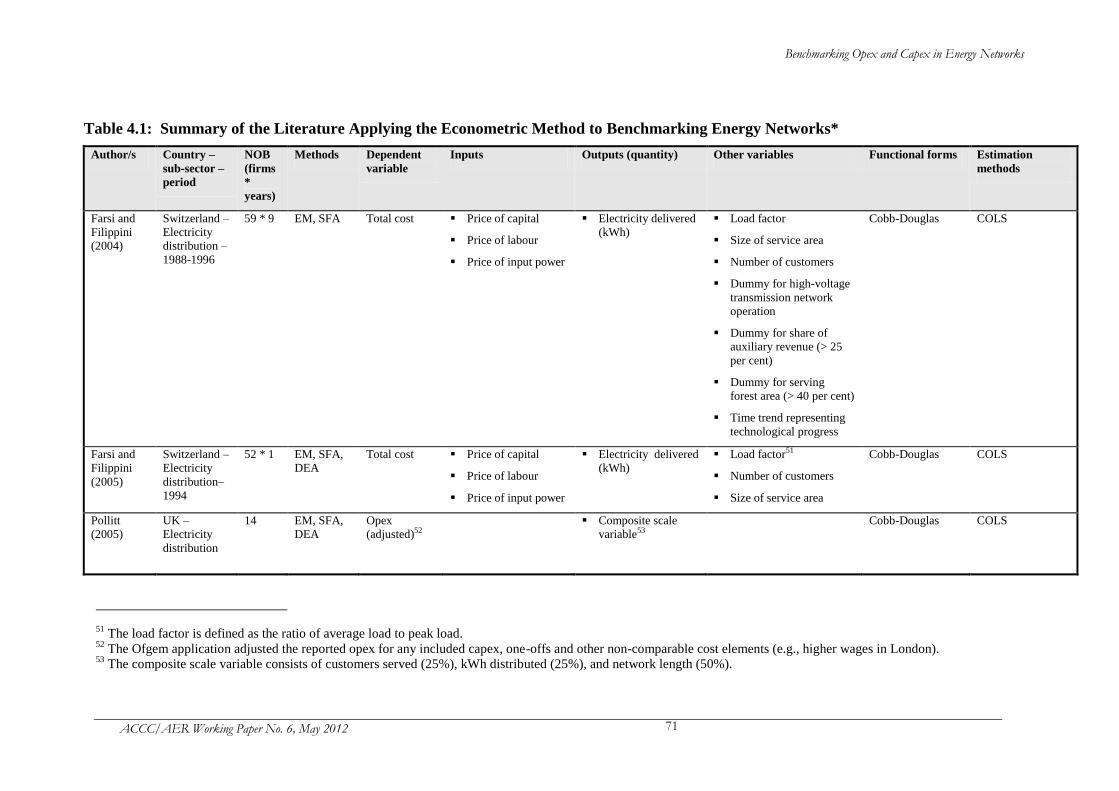
Benchmarking Opex and Capex in Energy Networks
ACCC/AER Working Paper No. 6, May 2012 71
Table 4.1: Summary of the Literature Applying the Econometric Method to Benchmarking Energy Networks*
Author/s Country –
sub-sector –
period
NOB
(firms
*
years)
Methods Dependent
variable
Inputs Outputs (quantity) Other variables Functional forms Estimation
methods
Farsi and
Filippini
(2004)
Switzerland –
Electricity
distribution –
1988-1996
59 * 9 EM, SFA Total cost Price of capital
Price of labour
Price of input power
Electricity delivered
(kWh)
Load factor
Size of service area
Number of customers
Dummy for high-voltage
transmission network
operation
Dummy for share of
auxiliary revenue (> 25
per cent)
Dummy for serving
forest area (> 40 per cent)
Time trend representing
technological progress
Cobb-Douglas
COLS
Farsi and
Filippini
(2005)
Switzerland –
Electricity
distribution–
1994
52 * 1 EM, SFA,
DEA
Total cost Price of capital
Price of labour
Price of input power
Electricity delivered
(kWh)
Load factor51
Number of customers
Size of service area
Cobb-Douglas
COLS
Pollitt
(2005)
UK –
Electricity
distribution
14 EM, SFA,
DEA
Opex
(adjusted)52
Composite scale
variable53
Cobb-Douglas COLS
51
The load factor is defined as the ratio of average load to peak load. 52
The Ofgem application adjusted the reported opex for any included capex, one-offs and other non-comparable cost elements (e.g., higher wages in London). 53
The composite scale variable consists of customers served (25%), kWh distributed (25%), and network length (50%).
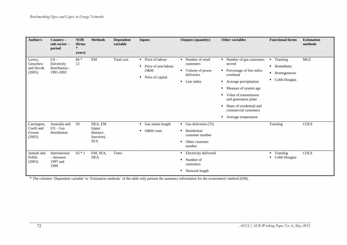
Benchmarking Opex and Capex in Energy Networks
ACCC/AER Working Paper No. 6, May 2012 72
Author/s Country –
sub-sector –
period
NOB
(firms
*
years)
Methods Dependent
variable
Inputs Outputs (quantity) Other variables Functional forms Estimation
methods
Lowry,
Getachew
and Hovde
(2005)
US –
Electricity
distribution –
1991-2002
66 *
12
EM Total cost Price of labour
Price of non-labour
O&M
Price of capital
Number of retail
customers
Volume of power
deliveries
Line miles
Number of gas customers
served
Percentage of line miles
overhead
Average precipitation
Measure of system age
Value of transmission
and generation plant
Share of residential and
commercial customers
Average temperature
Translog
Homethetic
Homogeneous
Cobb-Douglas
MLE
Carrington,
Coelli and
Groom
(2002)
Australia and
US – Gas
distribution
59 DEA, EM
(input
distance
function),
SFA
Gas mains length
O&M costs
Gas deliveries (TJ)
Residential
customer number
Other customer
number
Translog COLS
Jamasb and
Pollitt
(2003)
International
– between
1997 and
1999
63 * 1 EM, SFA,
DEA
Totex Electricity delivered
Number of
customers
Network length
Translog
Cobb-Douglas
COLS
* The columns ‘Dependent variable’ to ‘Estimation methods’ of the table only present the summary information for the econometric method (EM).
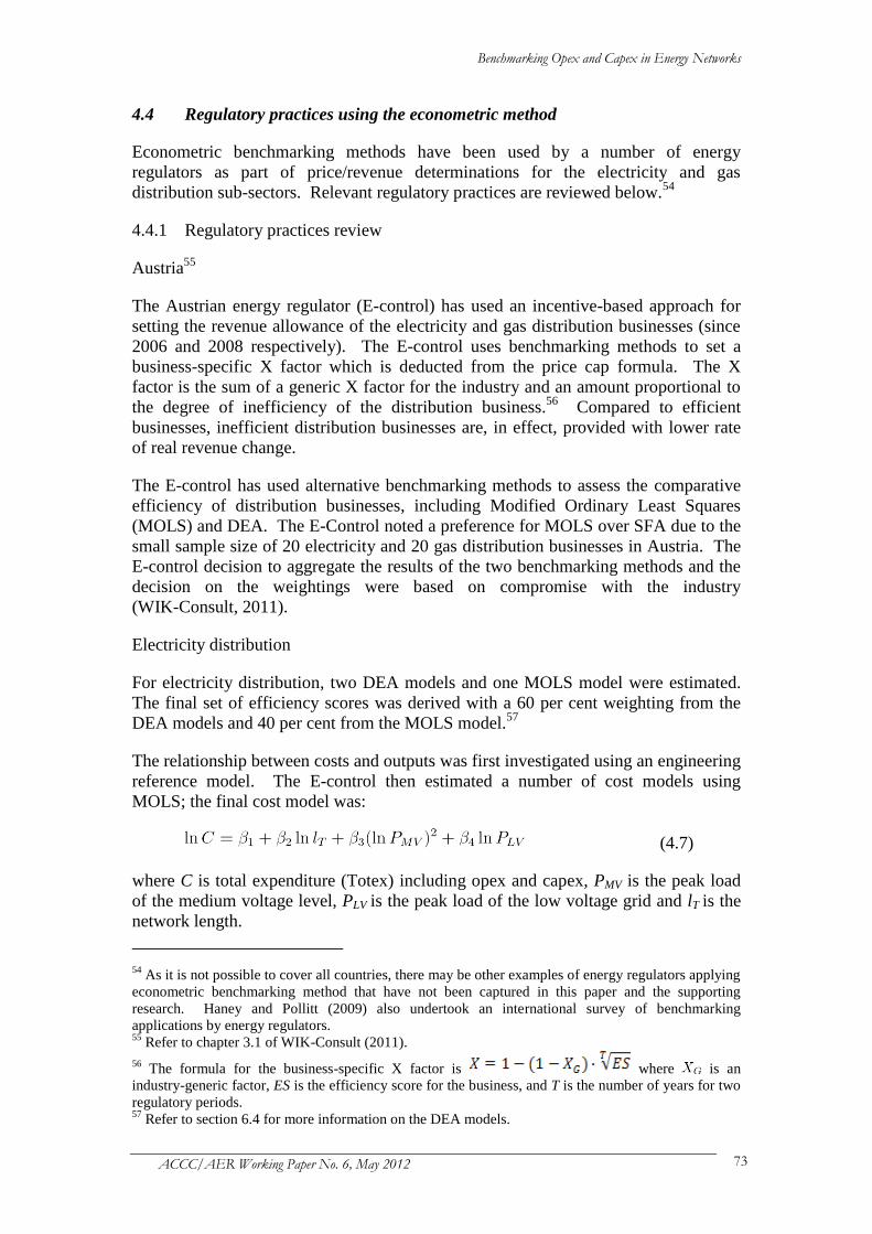
Benchmarking Opex and Capex in Energy Networks
ACCC/AER Working Paper No. 6, May 2012 73
4.4 Regulatory practices using the econometric method
Econometric benchmarking methods have been used by a number of energy
regulators as part of price/revenue determinations for the electricity and gas
distribution sub-sectors. Relevant regulatory practices are reviewed below.54
4.4.1 Regulatory practices review
Austria55
The Austrian energy regulator (E-control) has used an incentive-based approach for
setting the revenue allowance of the electricity and gas distribution businesses (since
2006 and 2008 respectively). The E-control uses benchmarking methods to set a
business-specific X factor which is deducted from the price cap formula. The X
factor is the sum of a generic X factor for the industry and an amount proportional to
the degree of inefficiency of the distribution business.56
Compared to efficient
businesses, inefficient distribution businesses are, in effect, provided with lower rate
of real revenue change.
The E-control has used alternative benchmarking methods to assess the comparative
efficiency of distribution businesses, including Modified Ordinary Least Squares
(MOLS) and DEA. The E-Control noted a preference for MOLS over SFA due to the
small sample size of 20 electricity and 20 gas distribution businesses in Austria. The
E-control decision to aggregate the results of the two benchmarking methods and the
decision on the weightings were based on compromise with the industry
(WIK-Consult, 2011).
Electricity distribution
For electricity distribution, two DEA models and one MOLS model were estimated.
The final set of efficiency scores was derived with a 60 per cent weighting from the
DEA models and 40 per cent from the MOLS model.57
The relationship between costs and outputs was first investigated using an engineering
reference model. The E-control then estimated a number of cost models using
MOLS; the final cost model was:
(4.7)
where C is total expenditure (Totex) including opex and capex, PMV is the peak load
of the medium voltage level, PLV is the peak load of the low voltage grid and lT is the
network length.
54
As it is not possible to cover all countries, there may be other examples of energy regulators applying
econometric benchmarking method that have not been captured in this paper and the supporting
research. Haney and Pollitt (2009) also undertook an international survey of benchmarking
applications by energy regulators. 55
Refer to chapter 3.1 of WIK-Consult (2011).
56 The formula for the business-specific X factor is where is an
industry-generic factor, ES is the efficiency score for the business, and T is the number of years for two
regulatory periods. 57
Refer to section 6.4 for more information on the DEA models.
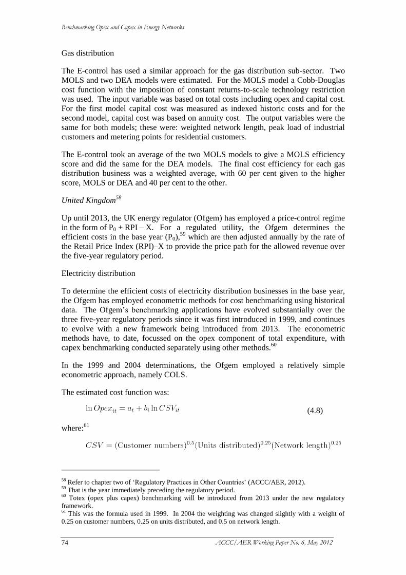
Benchmarking Opex and Capex in Energy Networks
ACCC/AER Working Paper No. 6, May 2012 74
Gas distribution
The E-control has used a similar approach for the gas distribution sub-sector. Two
MOLS and two DEA models were estimated. For the MOLS model a Cobb-Douglas
cost function with the imposition of constant returns-to-scale technology restriction
was used. The input variable was based on total costs including opex and capital cost.
For the first model capital cost was measured as indexed historic costs and for the
second model, capital cost was based on annuity cost. The output variables were the
same for both models; these were: weighted network length, peak load of industrial
customers and metering points for residential customers.
The E-control took an average of the two MOLS models to give a MOLS efficiency
score and did the same for the DEA models. The final cost efficiency for each gas
distribution business was a weighted average, with 60 per cent given to the higher
score, MOLS or DEA and 40 per cent to the other.
United Kingdom58
Up until 2013, the UK energy regulator (Ofgem) has employed a price-control regime
in the form of P0 + RPI – X. For a regulated utility, the Ofgem determines the
efficient costs in the base year (P0),59
which are then adjusted annually by the rate of
the Retail Price Index (RPI)–X to provide the price path for the allowed revenue over
the five-year regulatory period.
Electricity distribution
To determine the efficient costs of electricity distribution businesses in the base year,
the Ofgem has employed econometric methods for cost benchmarking using historical
data. The Ofgem’s benchmarking applications have evolved substantially over the
three five-year regulatory periods since it was first introduced in 1999, and continues
to evolve with a new framework being introduced from 2013. The econometric
methods have, to date, focussed on the opex component of total expenditure, with
capex benchmarking conducted separately using other methods.60
In the 1999 and 2004 determinations, the Ofgem employed a relatively simple
econometric approach, namely COLS.
The estimated cost function was:
(4.8)
where:61
58
Refer to chapter two of ‘Regulatory Practices in Other Countries’ (ACCC/AER, 2012). 59
That is the year immediately preceding the regulatory period. 60
Totex (opex plus capex) benchmarking will be introduced from 2013 under the new regulatory
framework. 61
This was the formula used in 1999. In 2004 the weighting was changed slightly with a weight of
0.25 on customer numbers, 0.25 on units distributed, and 0.5 on network length.
Benchmarking Opex and Capex in Energy Networks
ACCC/AER Working Paper No. 6, May 2012 75
For the 2009 determination, the Ofgem employed panel data regression techniques
using a time-fixed effects approach,62
and data covering 14 distribution businesses
over the four years from 2005-06 to 2008-09. The Ofgem undertook 40 regressions
using the log-log functional form. The 40 regressions covered three different levels of
disaggregation (total opex, single opex categories and groups of opex categories),
different combinations of included cost inputs, cost drivers (outputs), and weightings
(where composite drivers were used).
From each of the 40 regression results, the Ofgem calculated a business-specific
efficiency score based on the electricity distribution business’s actual costs compared
with the estimated efficient costs, which was then adjusted for the industry-average
efficiency score. These 40 efficiency scores were then weighted to give a single
score. The weightings were determined based on the Ofgem’s judgement.
Gas distribution
The Ofgem also commissioned benchmarking studies to assess efficient opex for the
gas distribution sub-sector. Regression benchmarking methods were employed to
benchmark total opex and direct opex categories. Indirect opex categories were
benchmarked using PPI methods (refer to section 2.4). The data used in the analysis
covered eight gas networks (in four ownership groups) for the two years 2005-06 and
2006-07.
The total opex benchmarking was undertaken by Europe Economics. Two COLS
models were estimated and given equal weighting. The input variable was total
controllable opex for both models. The output variables were: volume of gas
distributed for the first model and total number of customers for the second model.
Europe Economics tested these models against a range of other models including two
COLS models with a composite scale output variable, four DEA models and three
multi-lateral TFP models. The benchmark efficient business was set at the upper
quartile.
The direct opex benchmarking was undertaken by PB Power. PB Power undertook
both engineering-based analysis and regression analysis. The regression analysis
often included a composite scale output variable. The regression model was used to
for benchmarking when the r-squared value was 0.7 or greater. The benchmark
efficient business was set at the upper quartile.
The Ofgem primarily adopted the results of the disaggregated benchmarking (that is
the direct and indirect opex categories), but then applied an uplift to these results
based on the average difference between the disaggregated benchmarks and the total
opex benchmarks.
Ireland63
The Irish energy regulator (the Commission for Energy Regulation – CER) used both
econometric and PPI benchmarking methods (refer to section 2.4) to inform revenue
decision for its single electricity distribution business, ESBN, for the period 2011 to
2015. A simple form of regression analysis was used to benchmark ESBN against 14
62
This was done by including a dummy variable for each time period. 63
Refer to chapter three of ‘Regulatory Practices in Other Countries’ (ACCC/AER, 2012).
Benchmarking Opex and Capex in Energy Networks
ACCC/AER Working Paper No. 6, May 2012 76
electricity distribution businesses in the UK. The dependent variable was defined as
opex plus non-network capex (normalised to ensure that only activities were
comparable and to take account of differences in capitalisation policies). The sole
explanatory variable was a composite scale variable (CSV) consisting of customer
numbers, electricity distributed and network length. The CER concluded that the
ESBN’s costs were 7.5 per cent above the upper quartile of the UK distribution
business costs and 16 per cent above the efficiency frontier. The CER therefore ruled
on a reduction of 11 per cent in controllable opex.
Ontario, Canada64
As discussed in sections 2.4 and 3.4, the OEB has employed incentive-based price-
cap regulation for electricity distribution businesses since 2000. A key component of
the price-cap formula is the X factor which is the productivity-offsetting factor. The
X factor is composed of three parts: an estimate of industry-wide productivity change
estimated by the index-number-based TFP method (refer to section 3.4.) and a stretch
factor estimated by the combination of unit-cost (refer to section 2.4) and econometric
benchmarking methods.
The econometric model developed by the OEB’s consultant, PEG, employed data
from 86 electricity distribution businesses in Ontario between 2002 and 2006. A
double-log model with quadratic input price and output terms was used to model total
opex. A time trend variable was also included. The statistically significant dependent
variables were:
output quantity variables – number of retail customers, total retail delivery
volume, and total circuit of distribution line (kilometre); and
an input price index – calculated as weighted average of sub-indices for labour
prices and prices of miscellaneous inputs such as materials and services; and
environmental variables – percentage of underground lines, a binary variable if
most of the service territory is on the Canadian Shield and a measure of system
age.
Statistical tests were conducted to test the hypothesis that each electricity distribution
business was an average cost performer over the sample period. The businesses were
then assigned as being either:
a significantly superior performer, if test showed the business to be a
significantly better cost performer than the average; or
a significantly inferior performer, if test showed the business to be a
significantly worse cost performer than the average; or
an average cost performer, if the test showed the business was not significantly
different from the average.
These results were then combined with the rankings from the unit-cost analysis (top
quartile, middle two quartiles or bottom quartile) to form three final groups. Each
final group was assigned a value for the stretch factor, a lower value for the relatively
more efficient groups, which feeds into the X factor. The final groupings are
re-assessed each year as new data become available, enabling regrouping and thus, the
update of assigned stretch factor during the regulatory period.
64
Refer to chapter six of ‘Regulatory Practices in Other Countries’ (ACCC/AER, 2012).
Benchmarking Opex and Capex in Energy Networks
ACCC/AER Working Paper No. 6, May 2012 77
California, the United States65
In the US state of California, regulated energy utilities have sometimes submitted
cost-benchmarking analysis to the California Public Utilities Commission (CPUC) to
support an application to increase rates. For example, San Diego Gas and Electric
Company (SDG&E) engaged PEG to conduct an econometric analysis of the
company’s cost efficiency. This 2006 PEG study was summarised in Lowry and
Getachew (2009c).
PEG developed an econometric cost model for each of the gas and electricity
distribution services. The cost model for gas used data on 41 gas distributors in the
US from 1994 to 2004. The total cost of gas distribution, including operation and
maintenance expenses and the cost of gas plant ownership, was used as the dependent
variable. The independent variables included: three input price indices for labour,
non-labour operation and maintenance expenses, and capital services respectively;
two output quantity variables for number of retail customers and volume of retail
deliveries respectively; three business condition variables for the percentage of
distribution main not made of cast iron, the number of electricity customers served (to
reflect the degree of diversification), a binary variable reflecting high or low customer
density; and a time trend variable to capture technological change. The flexible trans-
log functional form was employed. The cost model for the 77 electricity distributors
in the US from 1994 to 2004 was similar to the gas model, with the total costs of
electricity distribution services estimated as a function of three input prices, two
output quantities and ten business condition variables.
PEG used the cost models to estimate the percentage difference between SDG&E’s
actual cost relative to the ‘efficient’ cost predicted by the model and then rank
SDG&E relative to the sample. The results formed part of SDG&E’s evidence in its
2008-2011 General Rate Case public hearing and settlement processes. Based on the
econometric cost analysis, SDG&E sought a stretch factor of zero (to apply to the gas
and electricity business as a whole).
Australian Energy Regulator (AER)
For the revenue determination for NSW and the ACT electricity distribution
businesses for the period 2009-10 to 2013-14, the AER’s consultant, Wilson Cook,
initially undertook PPI analysis using a composite size variable (refer to section 2.4).
Following criticisms of this approach, Wilson Cook employed regression analysis to
test the reasonableness of its bottom-up estimation of opex allowances (Wilson Cook,
2009, pp. 13-14). The dependent variable was opex and the explanatory variables
were number of customers, line length, maximum demand, energy distributed and
network type (urban or rural, based on customer density). Two models were
considered to predict opex, a linear combination of the available variables and a linear
combination of their log values. The data were based on 13 electricity distribution
businesses within the AER’s jurisdiction for the year of 2006-07. The AER (2009b,
p. 176) noted that the results of the regression model were ‘not materially different to
those of the original analysis’ and that this top-down analysis provides ‘a useful test
of the reasonableness of Wilson Cook’s bottom up assessment’.
65
Refer to chapter seven of ‘Regulatory Practices in Other Countries’ (ACCC/AER, 2012).

Benchmarking Opex and Capex in Energy Networks
ACCC/AER Working Paper No. 6, May 2012 78
A similar regression method was also applied by the AER as part of the assessment of
Queensland and South Australian determinations for the regulatory period 2010-11 to
2014-15. As described in section 2.4, the opex assessment was primarily undertaken
by consultant PB Australia focussing on a bottom-up engineering-based approach
with consideration of the PPI benchmarking analysis as a cross check.
4.4.2 Summary of regulatory practices
The above review provides some examples of energy regulators that have employed
econometric methods to determine the cost efficiency of energy networks operating in
electricity and gas distribution sub-sectors respectively. While the AER and the
Ontario, Austrian and Irish energy regulators combined the econometric results with
the results of other benchmarking methods,66
the UK energy regulator relied primarily
on the results of the econometric method.67
Other than Ontario, each of the above regulatory applications reviewed had 20 or
fewer distribution businesses that could be included in the sample. Notably none of
these regulators included many explanatory variables in the regression models.
Turvey (2006) and Pollitt (2005) have questioned the theoretical basis of the UK
benchmarking model used for the 1999 and 2004 price reviews. They argued against
the simple but arbitrary model as it did not: include different input prices, sufficiently
consider stochastic factors and consider the possible trade-off between capex and
opex. The Irish model was based on the 2004 UK model. Similarly, the Austrian
model was criticised by Turvey (2006) in that the small sample size could be the
reason for other cost drivers being found to be statistically insignificant.
In contrast, with a sample of 86 electricity distribution businesses, the Ontario
regulator was able to include a large number of explanatory variables, including
environmental variables in addition to multiple outputs and an input price index (in
linear and quadratic terms).
4.5 Issues arising from the review
There are a number of issues associated with the application of the conventional
econometric method to benchmarking. These issues relate to the choice of: the
functional form of the estimated cost function, explanatory variables included in the
cost function, the method for the estimation, and the interpretation of the results.
4.5.1 Choice of functional form
As discussed, functional forms such as the Cobb-Douglas function suffer from a lack
of flexibility compared to the translog functional form. That is, they restrict the
possible range of estimated outcomes. While their results may reflect the underlying
technology of the estimated industry, this is only the case if the underlying technology
falls within the subset of possibilities captured by these functional forms. That is, less
66
The CER informally combined the econometric results with the PPI benchmarking method results. 67
The Ofgem did, however, compare the results of the econometric method with DEA analysis using
the core model specifications for electricity distribution and with DEA and multilateral TFP analyses
using similar model specifications for gas distribution.
Benchmarking Opex and Capex in Energy Networks
ACCC/AER Working Paper No. 6, May 2012 79
flexible functional forms are less likely to yield results that approximate reality,
compared to the translog functional form.
The translog functional form, although more flexible than the simple Cobb-Douglas
function, still imposes restrictions on the range of possible cost functions. The choice
of functional form is not benign. For example, the translog function rules out the
possibility of: having zero values for one or some of the outputs and inputs specified;
or discontinuities and other irregularities in the cost function.
Regardless of the flexibility of the functional form used, if the true cost function does
not fit within the class of functions chosen, the resulting efficiency measurements can
be misleading.
4.5.2 Choice of explanatory variables
There are significant issues associated with the selection of outputs, input prices, and
environmental variables to be used in the model. For example, some argue that there
are limitations associated with measuring, aggregating and comparing variables such
as network capacity which can vary across each geographic location in the network.
Further, some argue that issues arise in relation to the measurement of capital
services.
There is not yet a consensus in the literature on the number or the set of variables
needed to fully capture all of the legitimate differences between the sampled energy
networks; for example, electricity distribution businesses. In general, the wider the
range of conditions faced by businesses in the sample, the larger the number of
variables required.
Figure 4.1 identifies the number of parameters in parametric benchmarking studies
(using one or both of conventional econometric method and SFA) published since
2000. This is compared with the number of businesses used in the studies. Several
features emerge. The two regulatory applications included on this chart (for Austria
and the UK) use a smaller sample size: 20 businesses in the case of Austria and 14 in
the case of the UK, and a correspondingly small number of parameters. Studies
which use a larger number of parameters generally use data from a larger number of
businesses. These studies also use panel data to increase the number of observations
in the study (Lowry, Getachew and Hovde 2005; Coelli, Crespo, Paszukiewicz,
Perelman, Plagnet and Romano 2008; and Estache, Rossi, and Ruzzier 2004). The
panel-data studies are located at the top right corner of this chart.
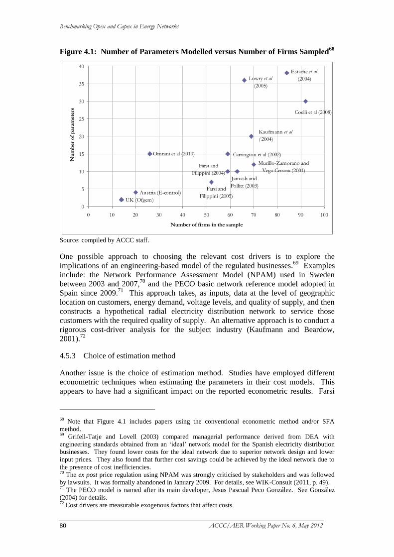
Benchmarking Opex and Capex in Energy Networks
ACCC/AER Working Paper No. 6, May 2012 80
Figure 4.1: Number of Parameters Modelled versus Number of Firms Sampled68
Farsi and
Filippini (2004)
Farsi and
Filippini (2005)
Lowry et al
(2005)
Murillo-Zamorano and
Vega-Cervera (2001)
Carrington et al (2002)
Coelli et al (2008)
Estache et al
(2004)
Jamasb and
Pollitt (2003)
Omrani et al (2010)
Austria (E-control)
UK (Ofgem)
0
5
10
15
20
25
30
35
40
0 10 20 30 40 50 60 70 80 90 100
Number of firms in the sample
Nu
mb
er
of
para
mete
rs
Kaufmann et al
( 2004)
Source: compiled by ACCC staff.
One possible approach to choosing the relevant cost drivers is to explore the
implications of an engineering-based model of the regulated businesses.69
Examples
include: the Network Performance Assessment Model (NPAM) used in Sweden
between 2003 and 2007,70
and the PECO basic network reference model adopted in
Spain since 2009.71
This approach takes, as inputs, data at the level of geographic
location on customers, energy demand, voltage levels, and quality of supply, and then
constructs a hypothetical radial electricity distribution network to service those
customers with the required quality of supply. An alternative approach is to conduct a
rigorous cost-driver analysis for the subject industry (Kaufmann and Beardow,
2001).72
4.5.3 Choice of estimation method
Another issue is the choice of estimation method. Studies have employed different
econometric techniques when estimating the parameters in their cost models. This
appears to have had a significant impact on the reported econometric results. Farsi
68
Note that Figure 4.1 includes papers using the conventional econometric method and/or SFA
method. 69
Grifell-Tatje and Lovell (2003) compared managerial performance derived from DEA with
engineering standards obtained from an ‘ideal’ network model for the Spanish electricity distribution
businesses. They found lower costs for the ideal network due to superior network design and lower
input prices. They also found that further cost savings could be achieved by the ideal network due to
the presence of cost inefficiencies. 70
The ex post price regulation using NPAM was strongly criticised by stakeholders and was followed
by lawsuits. It was formally abandoned in January 2009. For details, see WIK-Consult (2011, p. 49). 71
The PECO model is named after its main developer, Jesus Pascual Peco González. See González
(2004) for details. 72
Cost drivers are measurable exogenous factors that affect costs.
Benchmarking Opex and Capex in Energy Networks
ACCC/AER Working Paper No. 6, May 2012 81
and Filippini (2004) estimated the same cost function with the same set of explanatory
variables and the same set of parameters, using four different estimation methods,
namely COLS, random-effects GLS, random-effects MLE, fixed-effects estimation.
They found that the resulting efficiency scores were sensitive to the estimation
method used. Given the theoretical differences and different underlying assumptions
associated with the different estimation methods, this is not surprising, particularly
when a simple functional form, such as the Cobb-Douglas function assumed in Farsi
and Filippini (2004), is used.
While averaging results from different methods has been suggested in the literature
(e.g., Jamasb and Pollitt, 2003) and adopted in regulatory practices, Pollitt (2005,
p. 287) pointed out that inconsistent results cannot be reconciled merely by averaging
if individual sets of results are not that satisfactory.
A potential shortcoming associated with this conventional econometric method is that
business-specific inefficiency may be correlated with other variables in the model.
Variations in efficiency may be attributable to, for example, business size or operating
environments. That is, the assumption that the inefficiencies are independently and
identically distributed is no longer held. The absence of independence calls into
question the use of least-squares estimators commonly used for econometric analysis.
If the chosen variables fully capture the legitimate cost differences between
businesses and if the true cost function fits within the functional form chosen, then
recall equation 4.4:
(4.9)
for some choice of the parameters.
The best estimation method depends on the distribution of the disturbance term. The
simplest approach is to assume that the disturbance is independently and identically
distributed with zero mean and constant variance, and thus uncorrelated with the
explanatory variables. Under this assumption it is appropriate to use simple Ordinary
Least Squares (OLS) to estimate the values of the parameters .73
Given
independence, it is possible to use a GLS technique if the distribution of the
disturbance is unknown or to use MLE if non-homoscedastic distribution is assumed
(See for example, Schmidt and Sickles, 1984; Lowry, Getachew and Hovde, 2005).
With heteroscedasticity, OLS point estimates remain unbiased but inefficient while
statistical testing is no longer valid due to biased estimates of standard errors of the
coefficients.
However, if the inefficiency term u is correlated with explanatory variables in the
model, the above estimation methods result in biased estimates of the parameters and
the measured inefficiencies. As suggested by the literature (see for example, Schmidt
and Sickles 1984 and Kumbhakar and Lovell 2000), having access to sufficiently long
panel data may assist as some panel-data estimation methods (e.g., fixed-effects) do
not require the independence assumption.
73
Under classical assumptions, the OLS estimator is the best linear unbiased estimator of the
parameters.
Benchmarking Opex and Capex in Energy Networks
ACCC/AER Working Paper No. 6, May 2012 82
Another cause of the violation of the independence assumption is the ‘omitted
variable’ problem. If a variable that should be modelled as part of cost structure is
left out and this variable is correlated with other variables in the model, then the
estimation results are biased. This problem can be avoided by careful consideration
of model specification and conducting model-specification tests.
4.5.4 Interpretation of the results
Without allowing for the effects of random error term, the conventional econometric
method attributes the entire residual differential to cost inefficiency difference
between businesses. Depending on the estimation methods and sometimes involving
judgement call by the researchers and/or regulators, the efficient business is
determined and is benchmarked against to derive the cost inefficiency measure.
The approach relies fundamentally on careful consideration of the appropriate model
specifications (covering what variables to model and in what form, error distribution)
and suitable estimation methods (including the proper benchmarks), as well as quality
data that are relatively free of statistical noises. If there is a need to model both the
random error term and the inefficiency term, then the approach known as Stochastic
Frontier Analysis (SFA) should be considered.
4.6 Conclusions
Many regulators have sought to use some form of econometric approach to
benchmarking. According to the international surveys conducted by Jamasb and
Pollitt (2001) and Haney and Pollitt (2009), among the statistical benchmarking
methods, the econometric approach to benchmarking is second in popularity only to
Data Envelopment Analysis in regulatory practice.
This approach has the potential to provide an important insight into the relative
performance of businesses. However, the selection of the explanatory variables, the
functional form, and the best estimation method need to be considered carefully.
In practice, these techniques may mix any measurement of inefficiency with ‘noise’ in
the data itself. It is not possible to separate out these factors by examining the results
of a benchmarking study alone. To this end, the SFA method is recommended as it
explicitly accounts for the random error term in the modelling.
However, it may be possible to improve the credibility or reliability of a
benchmarking study through careful attention to a number of steps. The first step is to
identify a list of explanatory variables, at the outset, which can explain the key
differences in costs incurred by regulated businesses. Several recent papers (such as
Burns, Jenkins and Riechmann 2005 and Turvey 2006) have emphasised the
importance of careful independent assessment of the likely cost drivers and factors
affecting differences in costs. Kaufmann and Beardow (2001) pointed out the
importance of also understanding the impact of service quality and other business
conditions on cost.
The second step is to establish the basic shape of the cost function. As emphasised
above, there are no a priori grounds in economic theory for assuming that the cost
function of, say, an electricity distribution business can be represented as a Cobb-

Benchmarking Opex and Capex in Energy Networks
ACCC/AER Working Paper No. 6, May 2012 83
Douglas or translog function. Instead, engineering models and economic analysis
should be used to determine the basic shape of that function.74
The third step is to establish a large enough dataset of comparable businesses.
Although there are only a limited number of independent comparable businesses in
Australia, there are many hundreds of such businesses overseas. A priori there
appears to be no reason why electricity distribution businesses in, say, the US – which
supply similar services using similar underlying technology – cannot be compared to
electricity distribution businesses in Australia.75
A final step is to interact and co-operate with the industry stakeholders (service
providers and customers) to further refine and improve the choice of variables, the
quality of the data, the choice of functional form, and so on. Benchmarking is likely
to be an iterative process.
74
There is some academic work in this area. Lowry, Getachew and Hovde (2005) pointed to the
seminal article by Neuberg (1977) and contributions by Hjalmarsson and Veiderpass (1992), Salvanes
and Tjotta (1998) and Yatchew (2000). 75
Kaufmann and Beardow (2001) emphasised the importance of collecting data particularly on rural
distribution utilities, since ‘Australia has a significant number of distribution businesses that operate
under very rural conditions’. See also Lowry, Getachew, and Hovde (2005).
Benchmarking Opex and Capex in Energy Networks
ACCC/AER Working Paper No. 6, May 2012 84
Chapter 5 Evaluation of the parametric SFA method
5.1 Introduction
Stochastic Frontier Analysis (SFA) is an extended econometric method that can be used
in cost benchmarking analysis. SFA enables the estimation of a cost frontier, from
which actual costs incurred by businesses can be compared. SFA is similar to other
econometric cost models in that it specifies a functional form that relates costs to
outputs, input prices, and environmental factors.76
However, it differs from traditional
econometric approaches in two main ways. First, SFA focuses on estimating the cost
frontier representing the minimum costs rather than estimating the cost function
representing the ‘average’ business. Second, SFA aims to separate the presence of
random statistical noise from the estimation of inefficiency.
SFA has been widely applied by academic researchers to estimate and compare the cost
efficiency of energy networks in one jurisdiction or between jurisdictions. The results
have often been compared with results from other benchmarking methods such as Data
Envelopment Analysis (DEA) or Corrected Ordinary Least Squares (COLS).
SFA has been applied by a limited number of energy regulators. Germany and Finland
have applied the SFA method to assess the relative cost efficiency of energy businesses
and Sweden has applied SFA to assess industry-wide productivity changes over time.
The remainder of this chapter is organised as follows. A description of the SFA
method is provided in section 5.2. A summary of the academic applications of SFA to
the energy sector is provided in 5.3 and a summary of regulatory applications is
provided in 5.4. Section 5.5 discusses the potential issues associated with the
application of SFA and conclusions are drawn in section 5.6.
5.2 Description of the SFA method77
As discussed in chapter 4, the econometric approach is traditionally estimated using
Ordinary Least Squares or its variants, such as corrected or modified least squares.
This estimation process identifies the residuals from the modelling in one term. The
residuals are then used to identify relative efficiency of the businesses. That is, the
residuals capture departures of a business’s actual costs from the estimated cost
function.
The problem with the traditional econometric approach is that while the departure from
the estimated cost function may be an indication of inefficiency, it may also be due to
random statistical noise, or because of other reasons that are not related to the
management-controllable inefficiency.
SFA addresses this shortcoming by isolating business-specific inefficiencies from the
effects of random statistical noise. SFA separates the composite residuals into two
components: random error term and a term capturing ‘other departures from the
76
Environmental factors are either included directly in the cost model or indirectly as explanatory
variables for estimating the one-sided error term (discussed in more detail in section 5.2.1). 77
For detailed description of SFA methods, refer to Kumbhakar and Lovell (2000).
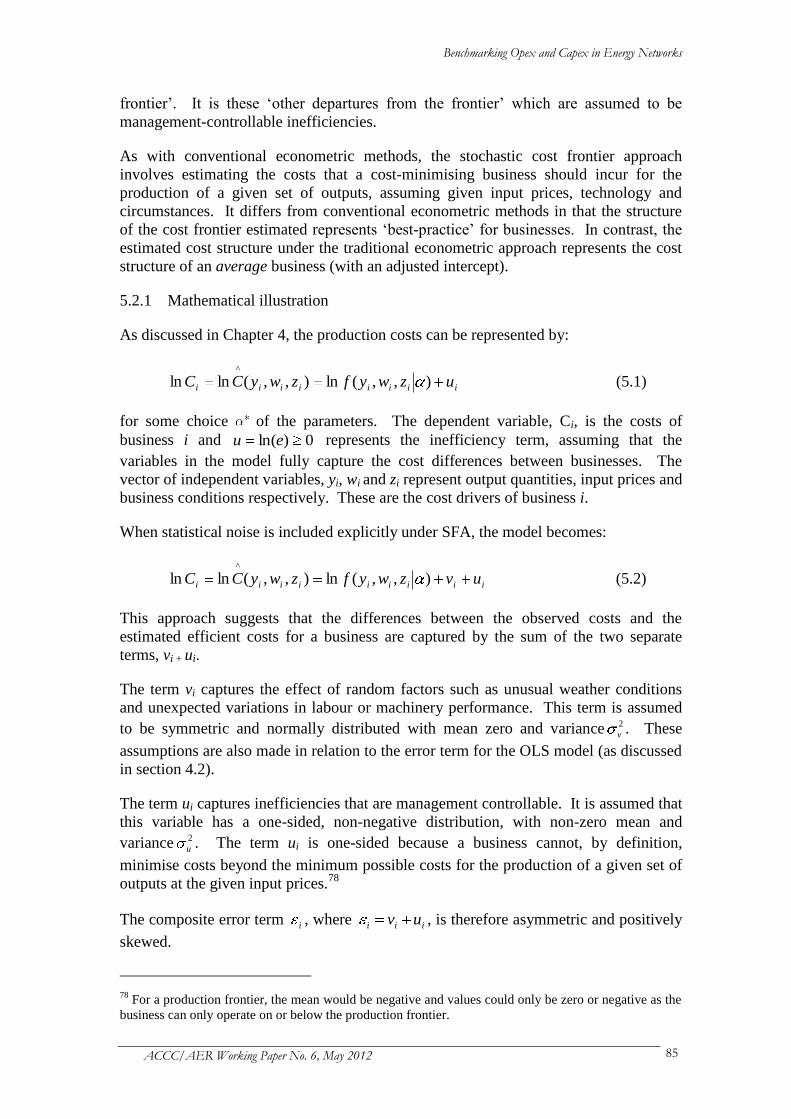
Benchmarking Opex and Capex in Energy Networks
ACCC/AER Working Paper No. 6, May 2012 85
frontier’. It is these ‘other departures from the frontier’ which are assumed to be
management-controllable inefficiencies.
As with conventional econometric methods, the stochastic cost frontier approach
involves estimating the costs that a cost-minimising business should incur for the
production of a given set of outputs, assuming given input prices, technology and
circumstances. It differs from conventional econometric methods in that the structure
of the cost frontier estimated represents ‘best-practice’ for businesses. In contrast, the
estimated cost structure under the traditional econometric approach represents the cost
structure of an average business (with an adjusted intercept).
5.2.1 Mathematical illustration
As discussed in Chapter 4, the production costs can be represented by:
iiiiiiii uzwyfzwyCC ),,(ln),,(lnln^
(5.1)
for some choice of the parameters. The dependent variable, Ci, is the costs of
business i and 0)ln(eu represents the inefficiency term, assuming that the
variables in the model fully capture the cost differences between businesses. The
vector of independent variables, yi, wi and zi represent output quantities, input prices and
business conditions respectively. These are the cost drivers of business i.
When statistical noise is included explicitly under SFA, the model becomes:
iiiiiiiii uvzwyfzwyCC ),,(ln),,(lnln^
(5.2)
This approach suggests that the differences between the observed costs and the
estimated efficient costs for a business are captured by the sum of the two separate
terms, vi + ui.
The term vi captures the effect of random factors such as unusual weather conditions
and unexpected variations in labour or machinery performance. This term is assumed
to be symmetric and normally distributed with mean zero and variance 2
v . These
assumptions are also made in relation to the error term for the OLS model (as discussed
in section 4.2).
The term ui captures inefficiencies that are management controllable. It is assumed that
this variable has a one-sided, non-negative distribution, with non-zero mean and
variance 2
u . The term ui is one-sided because a business cannot, by definition,
minimise costs beyond the minimum possible costs for the production of a given set of
outputs at the given input prices.78
The composite error term i , where iii uv , is therefore asymmetric and positively
skewed.
78
For a production frontier, the mean would be negative and values could only be zero or negative as the
business can only operate on or below the production frontier.
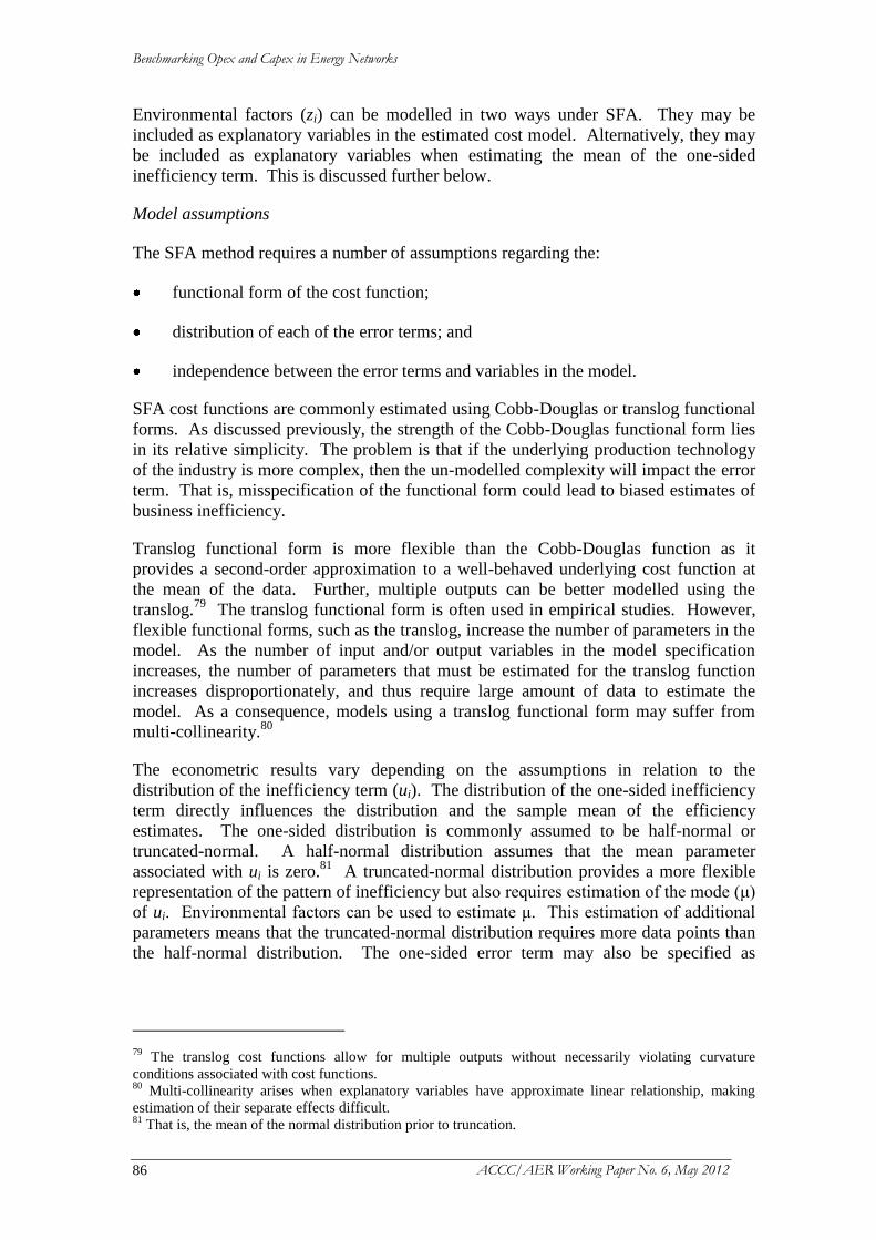
Benchmarking Opex and Capex in Energy Networks
ACCC/AER Working Paper No. 6, May 2012 86
Environmental factors (zi) can be modelled in two ways under SFA. They may be
included as explanatory variables in the estimated cost model. Alternatively, they may
be included as explanatory variables when estimating the mean of the one-sided
inefficiency term. This is discussed further below.
Model assumptions
The SFA method requires a number of assumptions regarding the:
functional form of the cost function;
distribution of each of the error terms; and
independence between the error terms and variables in the model.
SFA cost functions are commonly estimated using Cobb-Douglas or translog functional
forms. As discussed previously, the strength of the Cobb-Douglas functional form lies
in its relative simplicity. The problem is that if the underlying production technology
of the industry is more complex, then the un-modelled complexity will impact the error
term. That is, misspecification of the functional form could lead to biased estimates of
business inefficiency.
Translog functional form is more flexible than the Cobb-Douglas function as it
provides a second-order approximation to a well-behaved underlying cost function at
the mean of the data. Further, multiple outputs can be better modelled using the
translog.79
The translog functional form is often used in empirical studies. However,
flexible functional forms, such as the translog, increase the number of parameters in the
model. As the number of input and/or output variables in the model specification
increases, the number of parameters that must be estimated for the translog function
increases disproportionately, and thus require large amount of data to estimate the
model. As a consequence, models using a translog functional form may suffer from
multi-collinearity.80
The econometric results vary depending on the assumptions in relation to the
distribution of the inefficiency term (ui). The distribution of the one-sided inefficiency
term directly influences the distribution and the sample mean of the efficiency
estimates. The one-sided distribution is commonly assumed to be half-normal or
truncated-normal. A half-normal distribution assumes that the mean parameter
associated with ui is zero.81
A truncated-normal distribution provides a more flexible
representation of the pattern of inefficiency but also requires estimation of the mode (μ)
of ui. Environmental factors can be used to estimate μ. This estimation of additional
parameters means that the truncated-normal distribution requires more data points than
the half-normal distribution. The one-sided error term may also be specified as
79
The translog cost functions allow for multiple outputs without necessarily violating curvature
conditions associated with cost functions. 80
Multi-collinearity arises when explanatory variables have approximate linear relationship, making
estimation of their separate effects difficult. 81
That is, the mean of the normal distribution prior to truncation.
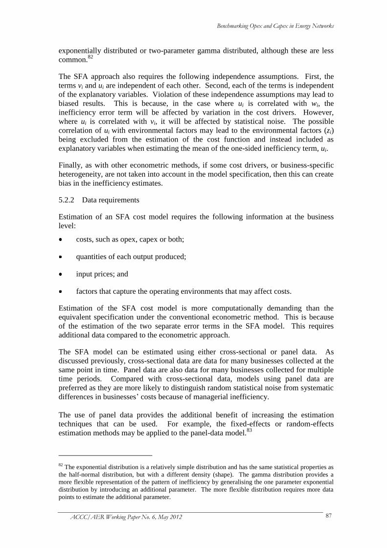
Benchmarking Opex and Capex in Energy Networks
ACCC/AER Working Paper No. 6, May 2012 87
exponentially distributed or two-parameter gamma distributed, although these are less
common.82
The SFA approach also requires the following independence assumptions. First, the
terms vi and ui are independent of each other. Second, each of the terms is independent
of the explanatory variables. Violation of these independence assumptions may lead to
biased results. This is because, in the case where ui is correlated with wi, the
inefficiency error term will be affected by variation in the cost drivers. However,
where ui is correlated with vi, it will be affected by statistical noise. The possible
correlation of ui with environmental factors may lead to the environmental factors (zi)
being excluded from the estimation of the cost function and instead included as
explanatory variables when estimating the mean of the one-sided inefficiency term, ui.
Finally, as with other econometric methods, if some cost drivers, or business-specific
heterogeneity, are not taken into account in the model specification, then this can create
bias in the inefficiency estimates.
5.2.2 Data requirements
Estimation of an SFA cost model requires the following information at the business
level:
costs, such as opex, capex or both;
quantities of each output produced;
input prices; and
factors that capture the operating environments that may affect costs.
Estimation of the SFA cost model is more computationally demanding than the
equivalent specification under the conventional econometric method. This is because
of the estimation of the two separate error terms in the SFA model. This requires
additional data compared to the econometric approach.
The SFA model can be estimated using either cross-sectional or panel data. As
discussed previously, cross-sectional data are data for many businesses collected at the
same point in time. Panel data are also data for many businesses collected for multiple
time periods. Compared with cross-sectional data, models using panel data are
preferred as they are more likely to distinguish random statistical noise from systematic
differences in businesses’ costs because of managerial inefficiency.
The use of panel data provides the additional benefit of increasing the estimation
techniques that can be used. For example, the fixed-effects or random-effects
estimation methods may be applied to the panel-data model.83
82
The exponential distribution is a relatively simple distribution and has the same statistical properties as
the half-normal distribution, but with a different density (shape). The gamma distribution provides a
more flexible representation of the pattern of inefficiency by generalising the one parameter exponential
distribution by introducing an additional parameter. The more flexible distribution requires more data
points to estimate the additional parameter.

Benchmarking Opex and Capex in Energy Networks
ACCC/AER Working Paper No. 6, May 2012 88
The fixed-effects technique, also known as the ‘within estimator’ technique, is a
superior estimation method where the inefficiency term ui is time invariant. That is, if
business-specific levels of inefficiency are assumed not to change over the sample time
period, then the fixed-effects technique provides more accurate estimations. Other
benefits include:
other assumptions in relation to the distribution of ui are not required;
assumptions in relation to the independence of ui relative to the cost drivers and
the independence of ui relative to vi are not required; and
parameter estimates are consistent as the sample size or time period increases.84
However, the fixed-effects technique:
assumes that at least one business in the sample is ‘fully efficient’. All other
businesses are then assessed relative to this ‘fully efficient’ business;
cannot accommodate explanatory variables that are time-invariant. For example,
it may not be appropriate to include environmental factors that have an impact on
costs but remain constant over time.
In the alternative, the random-effects estimation method can be applied in conjunction
with the generalised least squares (GLS) estimation procedure.85
The inefficiency error
term is random such that it is not correlated with independent variables. The benefits of
using the random-effects estimation technique include:
the possible inclusion of time-invariant cost drivers in the model;
assumptions about the distributional shape of ui are not required, except that ui is
non-negative and is randomly distributed with a constant mean and variance; and
the estimated parameters are consistent as the sample size and time period
increases.
The random-effects estimation method, however, does require the assumption that ui is
independent of vi and is independent of the explanatory variables of the model.
As with other econometric models, the longer the time period covered by the panel
data, the more likely that technology will change over time and affect the results. The
introduction of a time-period dummy variable can control, and provide an estimate for,
the effects of technical change over time.86
83
Variants of both the random- and fixed-effects models will also be available. 84
In this context, ‘consistency’ means that as more businesses or more time periods are included, the
distribution of the parameter estimates tightens around the expected value. 85
GLS is estimated first using OLS, then the parameter estimates are re-estimated using an econometric
technique called feasible generalised least squares. 86
See, for example, Hattori (2002) as reviewed in section 5.3.
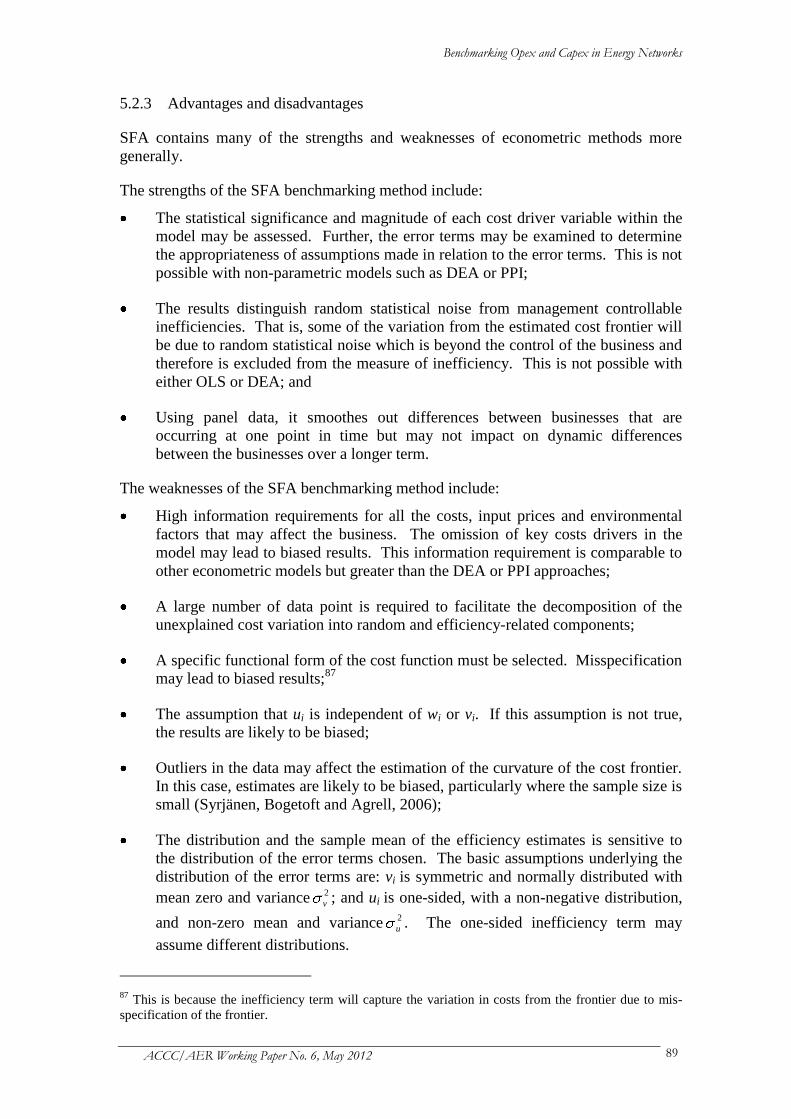
Benchmarking Opex and Capex in Energy Networks
ACCC/AER Working Paper No. 6, May 2012 89
5.2.3 Advantages and disadvantages
SFA contains many of the strengths and weaknesses of econometric methods more
generally.
The strengths of the SFA benchmarking method include:
The statistical significance and magnitude of each cost driver variable within the
model may be assessed. Further, the error terms may be examined to determine
the appropriateness of assumptions made in relation to the error terms. This is not
possible with non-parametric models such as DEA or PPI;
The results distinguish random statistical noise from management controllable
inefficiencies. That is, some of the variation from the estimated cost frontier will
be due to random statistical noise which is beyond the control of the business and
therefore is excluded from the measure of inefficiency. This is not possible with
either OLS or DEA; and
Using panel data, it smoothes out differences between businesses that are
occurring at one point in time but may not impact on dynamic differences
between the businesses over a longer term.
The weaknesses of the SFA benchmarking method include:
High information requirements for all the costs, input prices and environmental
factors that may affect the business. The omission of key costs drivers in the
model may lead to biased results. This information requirement is comparable to
other econometric models but greater than the DEA or PPI approaches;
A large number of data point is required to facilitate the decomposition of the
unexplained cost variation into random and efficiency-related components;
A specific functional form of the cost function must be selected. Misspecification
may lead to biased results;87
The assumption that ui is independent of wi or vi. If this assumption is not true,
the results are likely to be biased;
Outliers in the data may affect the estimation of the curvature of the cost frontier.
In this case, estimates are likely to be biased, particularly where the sample size is
small (Syrjänen, Bogetoft and Agrell, 2006);
The distribution and the sample mean of the efficiency estimates is sensitive to
the distribution of the error terms chosen. The basic assumptions underlying the
distribution of the error terms are: vi is symmetric and normally distributed with
mean zero and variance 2
v ; and ui is one-sided, with a non-negative distribution,
and non-zero mean and variance 2
u . The one-sided inefficiency term may
assume different distributions.
87
This is because the inefficiency term will capture the variation in costs from the frontier due to mis-
specification of the frontier.
Benchmarking Opex and Capex in Energy Networks
ACCC/AER Working Paper No. 6, May 2012 90
The SFA benchmarking method also sets the benchmark at the ‘frontier’. This is
similar to the DEA method. The frontier represents the minimum, optimised, level of
costs that a business will incur based on the most efficient business in the industry, to
produce a given set of outputs for a given set of input prices. In contrast, when
estimated by OLS, the econometric method estimates the cost function which is derived
from the ‘average’ business in the sample. Based on this function, the benchmark cost
frontier may then be shifted to place the business that is deemed to be efficient at the
frontier.88
5.3 Literature review of the SFA method
A review of the literature shows that the SFA method has been applied to
benchmarking the energy sector in a number of different ways. A sample of the
relevant literature is provided in this section. Many of the studies have focussed on
comparing the consistency of efficiency results across different benchmarking methods
including SFA, DEA and/or econometric methods. Similarly some studies have used
the SFA method only and assessed the consistency of results with respect to alternative
estimation methods or functional forms. Other studies have used SFA simply for
sensitivity analysis to test the robustness of efficiency estimates obtained through other
benchmarking methods. A summary of the findings of these studies is provided below.
For each empirical study in relation to energy networks, table 5.1 contains summary
information on the estimation methods, functional forms, inputs and outputs included in
the main model and the data employed.
5.3.1 SFA for primary analysis
Hattori (2002) used data covering 12 American and nine Japanese electricity
distribution businesses between 1982 and 1997 to estimate their comparative efficiency
performance. The author employed SFA to estimate the level of technical inefficiency
for each business in each year of the sample under four different SFA model
specifications, each of which included a different set of control variables on operating
environments. Data limitations prevented the inclusion of the ratio of overhead to
underground lines as an output variable, the inclusion of which the author considered
could enhance the study. The author found that the Japanese electric utilities were on
average more efficient than the utilities in the United States (US) and had lower
variation in efficiency. Inefficiencies appeared to be increasing over time and the
annual rate of technical change had a decreasing trend.
Gong and Sickles (1989) undertook an experimental analysis to explore the sensitivity
of SFA results to different functional form assumptions and different estimation
methods. The authors used Monte Carlo simulations to generate data that approximated
the following functional forms – the CES-translog, the translog and the generalised
Leontief. The authors then estimated business-specific technical inefficiencies using
three estimation methods, namely maximum likelihood, random effects (by generalized
least squares) and fixed effects (the within estimator). By comparing the estimated
inefficiency with assumed inefficiency, the authors found that the SFA approach is
sensitive to the form of the underlying technology. SFA is very good when the
underlying technology is very simple (e.g., Cobb-Douglas or CES) but this ability to
88
For example, if Corrected Ordinary Least Squares and Modified Ordinary Least Squares are used.
Benchmarking Opex and Capex in Energy Networks
ACCC/AER Working Paper No. 6, May 2012 91
accurately estimate inefficiency decreases as the underlying technology becomes more
complex. However they found that the performance of the three estimation methods
was similar, giving quite stable efficiency scores across estimation methods. The
authors noted a preference for the fixed-effects (within estimator) estimation as it
allows for weaker assumptions regarding the independence of outputs and technical
efficiency, and is computationally easier.
Farsi, Filippini and Kuenzle (2007) undertook an empirical study of the cost structure
of 26 gas distribution utilities operating in Switzerland from 1996 to 2000. The authors
tested the sensitivity of the cost efficiency scores estimated by SFA under four different
estimation methods, two MLE and two random-effects (GLS) procedures. The authors
found that while the efficiency estimates were reasonably robust to estimation method
and showed a strong correlation, the ‘best’ and ‘worst’ utilities identified change across
methods. The authors suggested that individual efficiency estimates cannot be directly
used to set the X factor in the price-cap formula.
In response to proposals to set the rates of electricity delivery equal to average
distribution costs in Switzerland, Filippini and Wild (1998) examined the scale and cost
efficiency of a sample of 30 Swiss electricity distribution businesses between 1992 and
1996 using SFA. They estimated an average-cost frontier model using the random-
effects procedure rather than a fixed-effects procedure, which was precluded due to one
of the environmental factors, size of service area, being fixed over time. Two cost
models with different input and output variables were estimated. The authors found the
existence of economies of output, customer density and scale, and that the majority of
Swiss electricity utilities were cost inefficient. They concluded that the average-cost
frontier model could be used to benchmark distributors and control the level of rates
proposed.
Filippini, Hrovatin and Zoric (2002) analysed the cost structure of Slovenian electricity
distribution businesses with respect to the cost and scale efficiency of the industry. The
study was based on data from five electricity distributors between 1991 and 2000.
Applying the SFA method to panel data, the authors estimated total costs as a function
of energy delivered, customer numbers, and capital and labour input prices. The authors
noted that, due to the small sample size, the translog model could not be considered and
therefore the Cobb-Douglas functional form was imposed. Similarly the small sample
size limited the inclusion of a larger set of explanatory variables. The authors noted
that the interpretation of the results should take into account the small sample size.
Nevertheless the authors considered that the analysis could be used by the Slovenian
regulator to increase the informational basis for more effective price-cap regulation.
The Finnish regulator (the Energy Market Authority – EMA) commissioned a report on
alternative benchmarking methods to DEA for measuring business-specific efficiency.
The EMA was concerned about a number of weaknesses with the DEA method,
including potential estimation errors caused by noise in the data, problems related to
exceptional businesses and the inability to formally analyse the choice of inputs,
outputs and environmental factors. The consultancy report, Syrjänen, Bogetoft and
Agrell (2006), considered 24 different input-output combinations and four different
functional-form specifications and compared the results using both the SFA and DEA
methods. The authors found that the SFA frontier was more stable over time than the
DEA frontier, the SFA model indicated no clear biases treating different sized
companies fairly, the SFA scores were higher than the DEA scores, and changes in
Benchmarking Opex and Capex in Energy Networks
ACCC/AER Working Paper No. 6, May 2012 92
efficiency scores are mostly caused by changes in an individual company’s inputs and
outputs. The authors considered the two benchmarking methods are complementary
such that the weaknesses of one benchmarking method are the strengths of the other
and vice versa. The authors therefore suggested that the SFA and DEA scores are
averaged to filter out potential mistakes relating to each method and would lead to
lower efficiency-change targets than DEA alone.
Kopsakangas-Sovolainen and Svento (2011) used panel data on 76 Finnish electricity
distribution businesses between 1997 and 2002 to estimate the impact on inefficiency
scores if observed and unobserved heterogeneity are taken into account in the SFA
modelling. The authors estimated five models, some of which account for observed
heterogeneity only and others which also take into account unobserved heterogeneity.
The authors found that both ways of accounting heterogeneity (observed or
unobserved) tended to diminish the inefficiency estimates and notably that the models
resulted in very different efficiency ranking of businesses.
Knittel (2002) used SFA to investigate the effect of alternative regulatory programs on
the technical efficiency of coal and natural gas generation units in the US. The data are
an unbalanced panel of generator-specific inputs and outputs for a large sub-set of
investor-owned utilities in the US covering the years 1981 to 1996. Noting a
preference of SFA over OLS, Knittel (2002) went on to test the SFA results using the
OLS method and found consistency in terms of sign and statistical significance.
Growitsch, Jamasb and Pollitt (2009) used SFA to estimate the efficiency of around
500 electricity distribution businesses from European countries. The authors focussed
on the impact of quality of services on efficiency and optimal business size. They
estimated a multi-output translog input distance function rather than a cost or revenue
function as the latter models require behavioural assumptions that may be violated.
They estimated two models, the first where total expenditure was driven by three output
variables and the second where quality of service, measured as customer minutes lost,
is included as an input. They found that large businesses may be better able to improve
service quality by increasing costs, while smaller businesses cannot substitute costs and
quality to the same extent.
5.3.2 SFA for comparison with other benchmarking methods
Burns and Weyman-Jones (1996) used panel data from electricity distribution
businesses in England and Wales to identify principal cost drivers, evaluate cost
efficiency performance, examine the impact of privatisation and assess the sensitivity
of the results to model specification and estimation method. The primary
benchmarking methods employed were SFA and OLS. First the authors compared the
OLS and SFA results using pooled cross-sectional time-series data and found little
difference between the results. However, once panel-data estimation were used, a
number of the explanatory variables become statistically insignificant and the final
model specification suggested operating costs depended only on the number of
customers, maximum demand and factor prices. The authors rejected the cross-
sectional and fixed-effects panel-data estimation methods in favour of the
random-effects estimation method. The authors also tested three different distributional
assumptions for the inefficiency error term, namely exponential, half-normal and
truncated-normal, and found little change in the efficiency rankings.
Benchmarking Opex and Capex in Energy Networks
ACCC/AER Working Paper No. 6, May 2012 93
Jamasb and Pollitt (2003) undertook an international benchmarking study of 63
electricity distribution and regional transmission businesses from six European
countries. The authors examined frontier-oriented benchmarking methods, including
DEA, COLS and SFA. They found that the choice of benchmarking method, model
specifications, and choice of variables could affect the efficiency scores as well as the
efficiency ranking of the businesses. While there was strong correlation between the
non-parametric and parametric methods, they found that the mean and minimum
efficiency scores in DEA were significantly lower than the SFA and COLS methods
when constant returns-to-scale technology was assumed. The correlation was weaker
when variable returns-to-scale technology was assumed. The SFA method also led to
higher estimated efficiency scores than the COLS method. The authors considered that
substantial variations in the scores and rankings from different methods were not
reassuring from a regulatory point of view and therefore a one-to-one translation of
efficiency scores to the X factor was not justified. They suggested that a practical
approach, in the absence of consensus on the most appropriate benchmarking method,
model specification, and variables, was to combine the results from different methods.
For example using the geometric mean of the scores of the preferred methods as this
tends to reduce the possible bias in individual methods.
Noting that DEA and SFA were the two most commonly-used frontier-based methods,
Estache, Rossi and Ruzzier (2004) used the two methods to estimate the efficiency of
84 South American electricity distribution businesses between 1994 and 2001. They
compared the results from two SFA models (an input distance function and an input
requirement function) and four DEA models (two input distance functions, one with
variable returns-to-scale and another with constant returns-to-scale, and two input
requirement functions, one with variable returns-to-scale and another with constant
returns-to-scale). The efficiency scores across the six models were found to be
statistically significantly different (based on the Kruskal-Wallis non-parametric test).
The authors considered that regulators should not directly translate efficiency scores to
the X factor. Mixed results, including inconsistency between DEA and SFA in
identifying the top and bottom performers, were found when testing the correlation in
the rankings between pairs of benchmarking methods. The authors suggested that
consistency in identifying efficient businesses is crucial, otherwise only a ‘mild’ form
of benchmarking should be relied on by regulators.
Farsi and Filippini (2004) measured the cost efficiency of 59 electricity distribution
utilities operating in Switzerland between 1988 and 1996. The authors considered
different frontier-based methods, including SFA and COLS, and compared the
efficiency scores and rankings across different models. The authors focussed on
parametric methods because of the ability to undertake statistical testing of the
significance of variables. The authors found that while the average inefficiency score
was not sensitive to the model chosen, the rankings varied significantly from one model
to another, possibly attributable to the unobserved heterogeneity among the distribution
utilities. Furthermore, the findings confirmed that the lack of robustness of efficiency
results reported in the previous literature was not limited to cross-sectional data. The
authors therefore considered that a direct use of inefficiency estimates in regulation
may be misleading and sensitivity analysis should be used to study the robustness of the
efficiency results, and the limitations of different models.
Benchmarking Opex and Capex in Energy Networks
ACCC/AER Working Paper No. 6, May 2012 94
Farsi and Filippini (2005) used a sample of 52 electricity distribution utilities in
Switzerland to assess the efficiency scores and ranks across alternative benchmarking
methods, namely COLS, SFA and DEA. Efficiency scores from COLS were six per
cent lower on average than the other methods, but the average estimates between DEA
and SFA were quite similar. There was a high correlation between SFA and COLS in
terms of both efficiency scores and rankings; however, the correlation with the DEA
efficiency scores and rankings was relatively low. Given the sensitivity of efficiency
scores to the benchmarking method employed, the authors recommended against using
the inefficiency estimates in a mechanical way, and instead suggested that
benchmarking analysis should be used as a complementary instrument in incentive
regulation.
Agrell and Bogetoft (2007) developed benchmarking models for the German electricity
and gas distribution upon request of the national regulator, Bundesnetzagentur
(BNetzA). The authors noted that, from a benchmarking perspective, Germany was
unique as there were a large number of distribution businesses and a large set of data
available on these, and the data were generally of good quality. This allowed for the
exploration of several benchmarking methods, DEA, SFA and OLS, under a range of
model specifications. The preliminary results showed similar cost efficiency rankings
and levels across the benchmarking methods. However, for gas distribution the authors
found that SFA performed in a more robust manner to data errors than DEA.
Coelli, Crespo, Paszukiewicz, Perelman, Plagnet and Romano (2008) estimated input
distance functions using SFA and DEA methods for a sample of 92 French electricity
distribution businesses over a three-year period. The purpose of this study is to
investigate the possibility of incorporating the quality of service in efficiency
benchmarking. Both DEA and SFA were used and consistency of the results across
methods was examined. The mean technical efficiency score was found to be similar
between the two models both with and without the inclusion of the quality measure.
The authors therefore concluded that the inclusion of the quality variable had no
significant effect upon mean technical efficiency scores for the given sample.
In a review paper by Kaufmann and Beardow (2001), alternative methods for
benchmarking electricity distributors, namely index-number-based TFP, econometric
cost function, SFA and DEA, were evaluated.. The authors found that econometric
techniques (such as econometric cost functions and SFA) had significant advantages
over DEA.
5.3.3 SFA for sensitivity testing
In 1999, the IPART commissioned London Economics to undertake a benchmarking
study of NSW electricity distribution businesses. In the study of London Economics
(1999), SFA was used for testing the sensitivity of the results derived from the primary
benchmarking method, DEA. The efficiency scores from the SFA and DEA methods
were compared in terms of the mean score, the scores and the ranking of businesses.
The study concluded that while there were some differences, the two benchmarking
methods gave sufficiently similar results.
Carrington, Coelli and Groom (2002) measured the technical efficiency of Australian
gas distributors relative to the US gas distribution businesses primarily using DEA.
SFA and COLS were then used to test the sensitivity of the DEA results with respect to

Benchmarking Opex and Capex in Energy Networks
ACCC/AER Working Paper No. 6, May 2012 95
method. The inclusion of the US sample for international benchmarking has enabled
estimation of the ‘data hungry’ SFA and DEA benchmarking methods. The SFA
assumed a translog functional form with variable returns-to-scale technology, and a
one-sided error term distributed as truncated normal. The parametric methods were
found to lead to lower efficiency scores because the frontiers bounded the data less
tightly than DEA. However the parametric methods produce results similar to the DEA
results. Because SFA recognises that some of the distance to the frontier is due to
random events or statistical noise, there were fewer efficient distribution businesses
identified, compared with the other benchmarking methods. Overall it was found that
the choice of benchmarking method had not unduly affected the efficiency scores.
5.3.4 Data used in academic studies
A number of academic studies carried out have used SFA to estimate the efficient
frontier. The number of explanatory variables and parameters vary between the studies
based on the purpose of the benchmarking study and the assumed technology
underpinning the production or cost function. In each instance, panel data for several
years or more are used. The number of observations used for each study is high. In
several cases, panel data for between 50 and 90 businesses are used. The length of
panel data is also longer where a smaller number of utilities is sampled in a study. For
example, Filippini, Hrovatin and Zoric (2002) used panel data for ten years in their
study of five electricity distribution businesses in Slovenia, while Burns and Weyman-
Jones (1996) used panel data for 13 years in their study of 12 electricity distribution
businesses in the United Kingdom (UK).
5.3.5 Conclusion on literature review
The use of SFA as a benchmarking method for estimating cost frontiers and
inefficiency is common in the academic literature. Much of this research has focussed
on the comparison of various SFA results, derived from different estimation methods
(e.g., panel versus cross-sectional data), different distributional assumptions and/or
different functional forms. Many studies have focussed on comparing the SFA method
with different benchmarking methods such as DEA and COLS. In many cases
significant differences in terms of the efficiency estimates and/or resulting business
ranking, between different benchmarking methods and between different SFA
specifications, were found. SFA has been used by some academics and by the German
and Finnish energy regulators as a primary method to benchmark cost efficiency. All
of these studies have used large samples of businesses and, where available, multiple
observations on the same business over time.
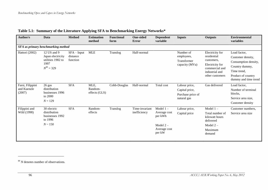
Benchmarking Opex and Capex in Energy Networks
ACCC/AER Working Paper No. 6, May 2012 96
Table 5.1: Summary of the Literature Applying SFA to Benchmarking Energy Networks*
Author/s Data Method Estimation
method
Functional
form
One-sided
Error
Dependent
variable
Inputs Outputs Environmental
variables
SFA as primary benchmarking method
Hattori (2002)
12 US and 9
Japan electricity
utilities 1982 to
1997
N89
= 329
SFA – Input
distance
function
MLE Translog Half-normal Number of
employees,
Transformer
capacity (MVa)
Electricity for
residential
customers,
Electricity for
commercial and
industrial and
other customers
Load factor,
Customer density,
Consumption density,
Country dummy,
Time trend,
Product of country
dummy and time trend
Farsi, Filippini
and Kuenzle
(2007)
26 gas
distribution
businesses 1996
to 2000
N = 129
SFA MLE,
Random-
effects (GLS)
Cobb-Douglas
Half-normal Total cost
Labour price,
Capital price,
Purchase price of
natural gas
Gas delivered
Load factor,
Number of terminal
blocks,
Service area size,
Customer density
Filippini and
Wild (1998)
30 electric
distribution
businesses 1992
to 1996
N ~ 150
SFA Random-
effects
Translog Time-invariant
inefficiency
Model 1 –
Average cost
per kWh
Model 2 –
Average cost
per kW
Labour price,
Capital price
Model 1 –
Total number of
kilowatt hours
delivered
Model 2 –
Maximum
demand
Customer numbers,
Service area size
89
N denotes number of observations.
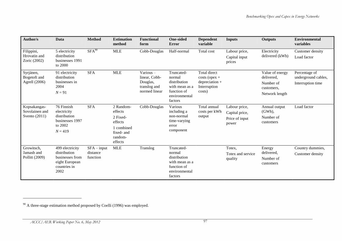
Benchmarking Opex and Capex in Energy Networks
ACCC/AER Working Paper No. 6, May 2012 97
Author/s Data Method Estimation
method
Functional
form
One-sided
Error
Dependent
variable
Inputs Outputs Environmental
variables
Filippini,
Hrovatin and
Zoric (2002)
5 electricity
distribution
businesses 1991
to 2000
SFA90
MLE Cobb-Douglas Half-normal Total cost Labour price,
Capital input
prices
Electricity
delivered (kWh)
Customer density
Load factor
Syrjänen,
Bogetoft and
Agrell (2006)
91 electricity
distribution
businesses in
2004
N = 91
SFA MLE Various –
linear, Cobb-
Douglas,
translog and
normed linear
Truncated-
normal
distribution
with mean as a
function of
environmental
factors
Total direct
costs (opex +
depreciation +
Interruption
costs)
Value of energy
delivered,
Number of
customers,
Network length
Percentage of
underground cables,
Interruption time
Kopsakangas-
Sovolainen and
Svento (2011)
76 Finnish
electricity
distribution
businesses 1997
to 2002
N = 419
SFA 2 Random-
effects
2 Fixed-
effects
1 combined
fixed- and
random-
effects
Cobb-Douglas Various
including a
non-normal
time-varying
error
component
Total annual
costs per kWh
output
Labour price,
Capital price,
Price of input
power
Annual output
(GWh),
Number of
customers
Load factor
Growitsch,
Jamasb and
Pollitt (2009)
499 electricity
distribution
businesses from
eight European
countries in
2002
SFA – input
distance
function
MLE Translog Truncated-
normal
distribution
with mean as a
function of
environmental
factors
Totex,
Totex and service
quality
Energy
delivered,
Number of
customers
Country dummies,
Customer density
90
A three-stage estimation method proposed by Coelli (1996) was employed.
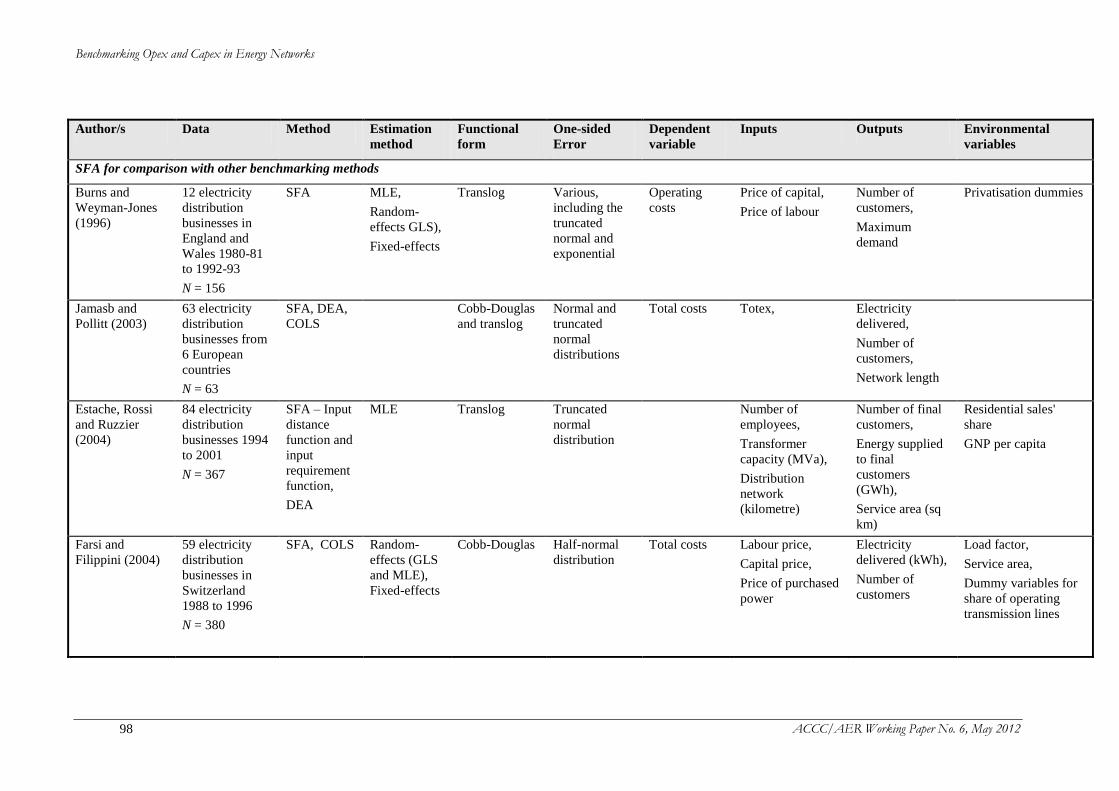
Benchmarking Opex and Capex in Energy Networks
ACCC/AER Working Paper No. 6, May 2012 98
Author/s Data Method Estimation
method
Functional
form
One-sided
Error
Dependent
variable
Inputs Outputs Environmental
variables
SFA for comparison with other benchmarking methods
Burns and
Weyman-Jones
(1996)
12 electricity
distribution
businesses in
England and
Wales 1980-81
to 1992-93
N = 156
SFA MLE,
Random-
effects GLS),
Fixed-effects
Translog Various,
including the
truncated
normal and
exponential
Operating
costs
Price of capital,
Price of labour
Number of
customers,
Maximum
demand
Privatisation dummies
Jamasb and
Pollitt (2003)
63 electricity
distribution
businesses from
6 European
countries
N = 63
SFA, DEA,
COLS
Cobb-Douglas
and translog
Normal and
truncated
normal
distributions
Total costs Totex,
Electricity
delivered,
Number of
customers,
Network length
Estache, Rossi
and Ruzzier
(2004)
84 electricity
distribution
businesses 1994
to 2001
N = 367
SFA – Input
distance
function and
input
requirement
function,
DEA
MLE Translog
Truncated
normal
distribution
Number of
employees,
Transformer
capacity (MVa),
Distribution
network
(kilometre)
Number of final
customers,
Energy supplied
to final
customers
(GWh),
Service area (sq
km)
Residential sales'
share
GNP per capita
Farsi and
Filippini (2004)
59 electricity
distribution
businesses in
Switzerland
1988 to 1996
N = 380
SFA, COLS Random-
effects (GLS
and MLE),
Fixed-effects
Cobb-Douglas Half-normal
distribution
Total costs Labour price,
Capital price,
Price of purchased
power
Electricity
delivered (kWh),
Number of
customers
Load factor,
Service area,
Dummy variables for
share of operating
transmission lines

Benchmarking Opex and Capex in Energy Networks
ACCC/AER Working Paper No. 6, May 2012 99
Author/s Data Method Estimation
method
Functional
form
One-sided
Error
Dependent
variable
Inputs Outputs Environmental
variables
Farsi and
Filippini (2005)
52 Swiss
electricity
distribution
businesses in
1994
N = 52
SFA, COLS,
DEA
MLE Cobb-Douglas Composite
half normal
distribution
Total costs Labour price,
Capital price,
Price of purchased
power
Total delivered
energy in kWh,
Number of
customers
Load factor,
Service area
Agrell and
Bogetoft (2007)
328
electricity
distribution
businesses
294 gas
distribution
businesses
COLS, SFA,
DEA
Translog
Truncated
normal
distribution
Total direct
cost
Service:
Number of
meters,
Service area (by
voltage)
Capacity:
Coincidental
load (by
voltage),
Transformer
(HS/MS,
MS/NS),
Feed-in power of
decentred
generation
N/A
Coelli, Crespo,
Paszukiewicz,
Perelman,
Plagnet and
Romano (2008)
92 electricity
distribution
businesses in
France over
three years
N = 276
SFA – input
distance
function,
DEA
MLE Translog Truncated
normal
distribution
Capital (gross
replacement
value),
Opex,
Total number of
interruptions
(quality variable)
Energy supplied,
Number of
customers,
Network length
(or service area)
Time-period dummies
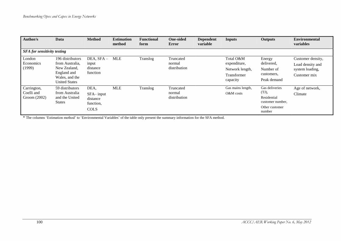
Benchmarking Opex and Capex in Energy Networks
ACCC/AER Working Paper No. 6, May 2012 100
Author/s Data Method Estimation
method
Functional
form
One-sided
Error
Dependent
variable
Inputs Outputs Environmental
variables
SFA for sensitivity testing
London
Economics
(1999)
196 distributors
from Australia,
New Zealand,
England and
Wales, and the
United States
DEA, SFA –
input
distance
function
MLE Translog Truncated
normal
distribution
Total O&M
expenditure,
Network length,
Transformer
capacity
Energy
delivered,
Number of
customers,
Peak demand
Customer density,
Load density and
system loading,
Customer mix
Carrington,
Coelli and
Groom (2002)
59 distributors
from Australia
and the United
States
DEA,
SFA– input
distance
function,
COLS
MLE Translog Truncated
normal
distribution
Gas mains length,
O&M costs
Gas deliveries
(TJ),
Residential
customer number,
Other customer
number
Age of network,
Climate
* The columns ‘Estimation method’ to ‘Environmental Variables’ of the table only present the summary information for the SFA method.
Benchmarking Opex and Capex in Energy Networks
ACCC/AER Working Paper No. 6, May 2012 101
5.4 Regulatory practices using the SFA method
5.4.1 Regulatory practices review
Energy regulators in Germany, Finland, and Sweden have applied the SFA
benchmarking method using data on electricity and/or gas distribution businesses to
either develop business-specific efficiency scores or estimate industry-wide
productivity change. The following information on the application of SFA by the
above regulators has been primarily drawn from WIK-Consult (2011).91
Germany92
Incentive regulation, via a revenue cap, was introduced in Germany in 2009. The new
revenue cap requires existing cost inefficiencies to be linearly removed over two
five-year regulatory periods. The national energy regulator, Bundesnetzagentur
(BNetzA), used cost benchmarking to determine the existing cost inefficiencies for
each of the 198 electricity distribution businesses and 187 gas distribution businesses
under the BNetzA’s jurisdiction.
The cost benchmarking was undertaken at the total cost level with no further
disaggregation of costs. The BNetA considered two different measures of total cost,
where the difference related to the measurement of capital costs. The first measure of
capital cost was based on the values reported from the utilities’ annual reports. The
second measure was based on a standardised cost of capital. The two different
measures of total cost were benchmarked using both SFA and DEA methods, therefore
resulting in four sets of cost inefficiency estimates for each business sampled.
The large number of distribution businesses in the sample enabled the BNetzA to
include a large number of output variables.
For electricity distribution, the same 11 variables were used for the four alternative
analyses. These were: number of connection points for high-, medium- and
low-voltage levels, circuit of cables (high and medium), circuit of lines (high and
medium), total network length (low), service area (low-voltage level), annual peak load
(high/medium and medium/low), number of transformer stations across all three
voltage levels, and installed capacity of distributed generation across all three voltage
levels. The first seven of the output variables captured end-user-related aspects and the
last four captured capacity-related aspects.
For gas distribution, the benchmarking included the same ten output variables for the
four alternative analyses. These were: number of exit points to end-users, number of
potential exit points to end-users, service area, pipeline length (≤ 5 bars and > 5 bars),
annual peak load, potential peak load, volume of pipelines, population in 1995 and
population in 2006. The first five of the output variables captured end-user-related
aspects and the last five captured capacity-related aspects.
91
There can be other examples of energy regulators applying SFA benchmarking methods. Haney and
Pollitt (2009) undertook an international survey of the current benchmarking applications by 40 energy
regulators. 92
Refer to chapter 3.4 of WIK-Consult (2011).
Benchmarking Opex and Capex in Energy Networks
ACCC/AER Working Paper No. 6, May 2012 102
To provide for flexibility in SFA model estimations, the BNetzA assumed normalised
linear cost functions with constant returns-to-scale and a truncated-normal distribution
of inefficiency. For the DEA models, however, non-decreasing returns-to-scale was
assumed to ensure that small distribution businesses were only compared with other
small distribution businesses. These functional forms were applied to both gas and
electricity.
The outcomes of the four models (two SFA and two DEA models) were combined by
setting the business-specific efficiency score as the maximum (most favourable) value
of the results if this was no less than 0.6; otherwise, 0.6 was applied. The identified
cost inefficiency for each utility is linearly deducted from the allowed revenue over two
five-year regulatory periods, such that by the end of the second period only the efficient
costs will be used to set the allowed revenue.
Finland93
In Finland, the 88 electricity distribution businesses are entitled to set their own tariffs,
but must follow the methods relating to opex and capex that are described ex ante by
the Finnish energy regulator, the Energy Market Authority (EMA). The EMA has
employed cost benchmarking since 2008 to set the individual efficiency targets for
opex. Both SFA and DEA methods were used because it became clear that both DEA
and SFA have some strengths and weaknesses.
For the regulatory period 2009 to 2011, the EMA considered that total-cost
benchmarking was most suitable as previous experience indicated that benchmarking
based on opex only created perverse incentives for regulated utilities to focus only on
controllable opex at the expense of other costs. The EMA measured total costs as the
overall costs to customers, comprised of operating costs, depreciation (straight line) and
the outage costs.94
The rationale for including outage costs was to prevent cost-cutting
at the expense of service quality. The same measure of total cost was used for both
SFA and DEA. The data were based on the average value of the cost inputs between
2003 and 2006.
In contrast to the BNetzA, the EMA only included a few output variables. For the SFA
method, these were total urban network length, total other network length, number of
users and value of energy distributed to consumption. The non-decreasing
returns-to-scale technology was assumed and the ‘linear functional form’
(Energiamarkkinavirasto, no date, p. 58) was used.
The outcomes of the two methods (SFA and DEA) were combined by taking a simple
average of efficiency scores from the two methods. The resulting business-specific
efficiency target indicates how much a business should reduce operating costs to
achieve an efficient cost level under the prescribed opex method.
93
Refer to chapter 3.3 of WIK-Consult (2011). 94
The outage cost measure appears to be a payment or rebate to customers following outages.

Benchmarking Opex and Capex in Energy Networks
ACCC/AER Working Paper No. 6, May 2012 103
Sweden95
Commencing in 2012, the Swedish regulator, the Energy Market Inspectorate (EI)
applies new ex ante incentive-based regulatory framework (revenue cap) to electricity
distribution. This new framework replaces an engineering-based reference model that
was used from 2003. Sweden has around 170 electricity distribution businesses.
The EI employed SFA, DEA and regression methods to analyse industry-wide
productivity change of electricity distribution businesses between 2001 and 2008. The
model consisted of controllable operating cost as the input variable and three output
variables, namely number of customers, length of lines and cables, and installed
capacity of transformers. The EI considered that there was no need to incorporate other
business environment variables as the focus was to estimate the industry-wide
productivity and not to compare utilities (WIK-Consult, 2011, p. 51). The EI used this
model to estimate an industry-wide efficiency target which is to be applied to
controllable operating costs only and therefore feed through into allowed revenue.96 No
benchmarking has been undertaken to set business-specific efficiency targets.
5.4.2 Summary of regulatory practices
This review has identified only a limited number of energy regulators that have used
SFA for cost benchmarking. Sweden, Germany and Finland all have a relatively large
number of distribution businesses, which has facilitated the use of SFA. Germany, with
over 180 distribution businesses in both gas and electricity, was able to include a large
number of dependent variables in their modelling. With 88 electricity distribution
businesses in Finland, the smaller sample size limited the number of output variables
that could be included in the model. All the three European regulators combined the
SFA benchmarking method with the use of other benchmarking methods such as DEA
and regression.
A number of other regulators such as the Ofgem (the UK energy regulator) and the
Dutch Energy Regulator, have considered but been advised against the use of the SFA
method for cost benchmarking by their consultants. This has been due to data
limitations resulting from the small number of regulated utilities, 14 electricity
distribution businesses in the UK and around 20 in the Netherlands. Similarly, Austria
ruled out SFA due to its relatively small sample of 20 gas and 20 electricity distribution
businesses.
5.5 Issues arising from the review
The review of the SFA method for the purpose of cost benchmarking, as covered in the
previous sections, includes the theory behind SFA, the empirical applications of SFA
by researchers mostly in the context of the energy sector, and by energy sector
regulators.
The key issues arising from this review are:
the need for extensive data to undertake the modelling;
95
Refer to chapter 3.7 of WIK-Consult (2011). 96
There is no further information available from WIK-Consult (2011) on how the results from different
methods were combined.
Benchmarking Opex and Capex in Energy Networks
ACCC/AER Working Paper No. 6, May 2012 104
the assumptions that must be made in relation to the choice of the functional form,
the distribution of the error terms and the independence of the error term and the
explanatory variables; and
the limited number of studies undertaken by regulators.
5.5.1 Data requirements
The SFA cost frontier model requires the following data: costs, output quantities, input
prices and business environmental conditions. Input quantities and cost share data may
also be required (Kumbhakar and Lovell, 2000). A mis-specification of the model,
where not all the relevant variables that determine the costs modelled are included, may
lead to the estimation of an incorrect cost frontier and biased estimates.
SFA also requires more data points than the conventional econometric methods in order
to estimate the two separate residual terms, namely the statistical noise term and the
inefficiency term. Without a large amount of data, the SFA method may not be able to
estimate all necessary explanatory variables based on the desired functional form. This
may result in a model misspecification error and a biased estimation of the cost
function.
In order to undertake SFA, a large sample size (by including utilities in other countries
or using panel data) is required. Given the small number of Australian businesses in
each of the energy sub-sectors, the sample size may be enlarged by including
comparable businesses in comparator countries.
Construction of a panel dataset requires data on the same businesses to be collected
repeatedly over time. The collected data must be consistent and directly comparable
over time. Data on the same businesses over time can also improve the separation of
statistical noise from estimated management-controllable inefficiency, and enable more
consistent estimation of the model parameters and the inefficiency term.
However, potential data issues may arise from the use of international benchmarking
and/or panel data. This is covered in Chapter 7.
5.5.2 Required assumptions
The SFA method requires that assumptions are made regarding the functional form of
the model. If the simpler Cobb-Douglas function is assumed for the production
technology, this risks biased estimation of the inefficiency term as the inefficiency
estimate may capture the departure of observed costs from the estimated frontier that is
due to technological factors left out of the model. As discussed in Chapter 4, the
translog model, while more flexible, requires considerably more data points. This is
particularly important as the number of parameters for estimation increases
disproportionately with the rise in the number of cost drivers. Similarly, other flexible
functional forms are data-intensive.
The SFA method also requires an assumption in relation to the one-sided inefficiency
error term. Empirical applications have tended to assume either the half-normal or
truncated-normal distributions to represent the pattern of inefficiency. While there is
no consensus on the appropriate specification, there does appear to be some early
Benchmarking Opex and Capex in Energy Networks
ACCC/AER Working Paper No. 6, May 2012 105
evidence suggesting that different distributions may not have significant effect on the
efficiency or accuracy of the results (Kumbhakar and Lovell, 2000, p. 90).
Finally, most of the SFA estimation methods, including MLE and random effects, still
require the assumption that the inefficiency error term is uncorrelated with the cost
drivers included in the model. However, in some cases this assumption may seem
counterintuitive. A violation of this independence assumption may lead to biased
estimation of both the inefficiency term, and the parameters of the cost drivers included
in the model.
5.5.3 Limited regulatory applications
The review of regulatory practices has identified three regulatory applications of SFA.97
Both Germany and Finland used SFA to determine the cost inefficiency of each
individual business. However, neither of these two regulators relied solely on the SFA
method. The German regulator applied the most favourable efficiency score derived
from four models; two models using SFA and two using DEA. The most favourable
efficiency score from the four models, if no less than 0.6, was applied. The Finnish
regulator averaged the results of two models; one estimated by SFA and the other by
DEA. Both regulators directly incorporated the identified inefficiency (relative to the
frontier) into the allowed revenue (for Germany) or operating cost method (for
Finland).
Sweden relied on SFA, together with econometric analysis and DEA, to determine the
industry-wide productivity change for controllable opex. This industry-wide efficiency
target feeds into the annual revenue allowance via the annual adjustments to the
efficient controllable operating costs.
All three of these European energy regulators have a large sample of utilities under
their jurisdictions. Germany and Sweden had over 170 utilities and Sweden also had
used panel data. Finland had 88 utilities and was not able to include many cost drivers
due to this relatively smaller sample size.
It is also important to note that the application of cost benchmarking in each of these
three European countries is relatively new. It was introduced in 2008, 2009 and 2012
for Finland, Germany and Sweden respectively. Indeed, it may be premature to draw
lessons from these experiences.
5.6 Conclusions
SFA has many desirable properties which lend well to cost benchmarking. In
particular, the separation of statistical noise from the estimation of management
controllable deviations from the cost frontier would seem appropriate in a regulatory
context. In addition, SFA retains many of the desirable properties of other econometric
methods including allowing for statistical testing of the model parameters, explanatory
power of variables and the error assumptions.
97
A number of energy regulators from the OECD countries have been reviewed. An international survey
by Haney and Pollitt (2009) also identified Belgium, Portugal and Norway as applying the SFA
benchmarking method in the most recent price review.
Benchmarking Opex and Capex in Energy Networks
ACCC/AER Working Paper No. 6, May 2012 106
However, SFA is a data-intensive benchmarking method and failure to include
sufficient data points for the estimation can lead to biased and/or inconsistent
estimation of the parameters in the model and, therefore, the estimated inefficiency
term. Most academic or regulatory applications of SFA have involved substantial data
points.
Similar to other econometric methods, SFA requires the imposition of assumptions
regarding functional form, the distribution of the error terms, including the one-sided
error term and the independence of the one-sided error term with all of the output
variables included in the model. Violation of these assumptions can lead to biased
estimation of the inefficiency term.
Given these potential issues, it would seem that the use of the SFA method to
benchmark cost efficiency for regulatory applications should be approached with
caution. Ideally, multiple periods of data on a large number of energy businesses in a
sub-sector would be available for the analysis. In addition it may be prudent to follow
the approach of academics and regulators that have applied the SFA benchmarking
method. That is to undertake cross-checking of the SFA efficiency or productivity
estimates (or rankings) against different model specifications and assumptions, and
against different benchmarking methods such as DEA, OLS and its variants.
Benchmarking Opex and Capex in Energy Networks
ACCC/AER Working Paper No. 6, May 2012 107
Chapter 6 Evaluation of the non-parametric DEA method
6.1 Introduction
Data Envelopment Analysis (DEA) is a technique that compares the efficiency and
productivity of businesses that produce similar outputs using similar inputs. Unlike
other parametric techniques, DEA does not require ex ante assumptions about the
shape of the underlying production function or cost function. Information about the
shape of the real-world production technology is inferred from observations of the
input-output combinations used by the businesses.
At the heart of DEA is a set of assumptions about how observed input-output
combinations from real-world businesses can provide information about the set of
possible input-output combinations available to the businesses in the industry. That
is, this approach relies on data in relation to the output levels of businesses in the
industry and the amount of inputs to produce that output (the ‘input-output
combinations’). Sophisticated mathematical techniques are employed to calculate
efficiency levels for each business, given their relative scale, output levels, output
mix, and use of inputs. That is, possible ‘input-output combinations’ are derived and
compared with actual input-output combinations so that the business-specific level of
efficiency is calculated. Different approaches to DEA differ in the assumptions about
the space of feasible input-output combinations from observations of the actual input-
output combinations achieved by individual businesses.
Once all possible input-output combinations are determined, the efficiency score for
each business is determined. Under the input-oriented version of this approach, the
efficiency score provides an answer to the following question: How much can the
inputs used by that business (holding the output constant) be scaled down and still
have an input-output combination which is feasible? The output-oriented version of
this approach asks: How much can the output of the business (holding the inputs
constant) be scaled up and still have an input-output combination which is feasible?
DEA is relatively simple and intuitive, and has been widely applied in practice. Many
academic papers relate to the theory or the applications of DEA. This body of
research covers a wide range of sectors. Scores of papers relate to the application of
DEA in public utility industries. Many economic regulators have applied DEA to
electricity and gas distribution companies as part of their regulatory processes.
The remainder of this chapter is structured as follows: section 6.2 describes the DEA
method in more detail. Section 6.3 reviews the academic literature on DEA and
section 6.4 reviews the regulatory practices which have used DEA. Section 6.5
discusses issues that arise in the application of DEA, and conclusions are drawn in
section 6.6.
6.2 Description of the DEA method
6.2.1 Method
The DEA method constructs a space of feasible input-output combinations starting
from observed input-output combinations of sample businesses. Different DEA
Benchmarking Opex and Capex in Energy Networks
ACCC/AER Working Paper No. 6, May 2012 108
approaches make different assumptions in extrapolating from specific observed input-
output combinations to the set of all possible feasible input-output combinations.
If a business produces the vector of N outputs using the vector of
M inputs x , the input-output combination is said to be
feasible. A sample of such observations yields a set of discrete feasible input-output
combinations , where S is the number of businesses.
From this observed set of feasible input-output combinations, the next step is to
extrapolate to the full space of feasible input-output combinations. The most common
approach to DEA is to assume:
Free disposability: If is a feasible combination then so is where
and ;98
and
Scalability and combinability of peer observations: If is a set of feasible
combinations, then so is where, under the assumption of
constant returns-to-scale (CRS), the weights of peer observations in forming the
surface of feasible input-output combination s are allowed to be any non-
negative real number.
Other assumptions may include:
the businesses have decreasing returns-to-scale (DRS), where the weights are
allowed to be any non-negative real number which sums to less than or equal to
one; or
the businesses have variable returns-to-scale (VRS) where the weights are
allowed to be any non-negative real number which sum to the value of one.
Given the set of feasible input-output combinations constructed, the DEA score for a
business under an input-oriented model is a measure of how much, for a given set of
outputs, the inputs used by the business could be proportionally scaled down while
still remaining within a space of feasible input-output combinations. Alternatively,
the output-oriented approach asks how much the output of the business could be
scaled up, holding the inputs constant, while still remaining within the space of
feasible input-output combinations.
The following description of the DEA method is based on an input-oriented model as
it is perceived to be appropriate for modelling electricity distribution, where
businesses may have less discretion over the output quantities supplied relative to the
inputs used. One could argue that capital inputs are fixed in the short run in
electricity distribution, as assumed in a number of DEA studies including London
Economics (1999). This requires the modelling of capital as the non-discretionary
input. For simplicity, this is not illustrated in the description below.
98 A vector y is said to be less than or equal to a vector if and only if every element of the first vector
is less than or equal to the corresponding element of the second vector.
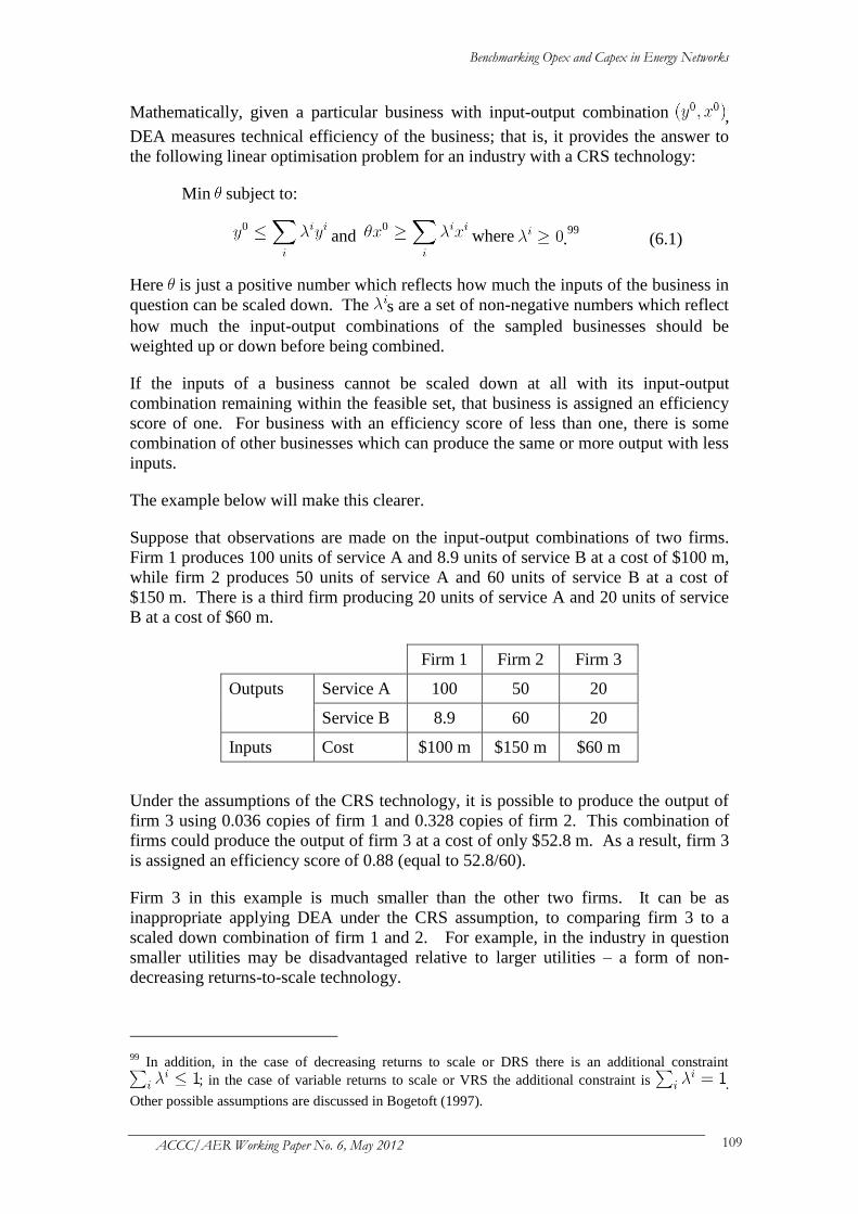
Benchmarking Opex and Capex in Energy Networks
ACCC/AER Working Paper No. 6, May 2012 109
Mathematically, given a particular business with input-output combination ,
DEA measures technical efficiency of the business; that is, it provides the answer to
the following linear optimisation problem for an industry with a CRS technology:
Min subject to:
and where .99
(6.1)
Here is just a positive number which reflects how much the inputs of the business in
question can be scaled down. The s are a set of non-negative numbers which reflect
how much the input-output combinations of the sampled businesses should be
weighted up or down before being combined.
If the inputs of a business cannot be scaled down at all with its input-output
combination remaining within the feasible set, that business is assigned an efficiency
score of one. For business with an efficiency score of less than one, there is some
combination of other businesses which can produce the same or more output with less
inputs.
The example below will make this clearer.
Suppose that observations are made on the input-output combinations of two firms.
Firm 1 produces 100 units of service A and 8.9 units of service B at a cost of $100 m,
while firm 2 produces 50 units of service A and 60 units of service B at a cost of
$150 m. There is a third firm producing 20 units of service A and 20 units of service
B at a cost of $60 m.
Firm 1 Firm 2 Firm 3
Outputs Service A 100 50 20
Service B 8.9 60 20
Inputs Cost $100 m $150 m $60 m
Under the assumptions of the CRS technology, it is possible to produce the output of
firm 3 using 0.036 copies of firm 1 and 0.328 copies of firm 2. This combination of
firms could produce the output of firm 3 at a cost of only $52.8 m. As a result, firm 3
is assigned an efficiency score of 0.88 (equal to 52.8/60).
Firm 3 in this example is much smaller than the other two firms. It can be as
inappropriate applying DEA under the CRS assumption, to comparing firm 3 to a
scaled down combination of firm 1 and 2. For example, in the industry in question
smaller utilities may be disadvantaged relative to larger utilities – a form of non-
decreasing returns-to-scale technology.
99
In addition, in the case of decreasing returns to scale or DRS there is an additional constraint
; in the case of variable returns to scale or VRS the additional constraint is .
Other possible assumptions are discussed in Bogetoft (1997).

Benchmarking Opex and Capex in Energy Networks
ACCC/AER Working Paper No. 6, May 2012 110
The conventional way in DEA to handle an alternative technology to CRS is to
impose a new constraint on the way that the space of feasible input-output
combinations is formed. Specifically, whereas the standard CRS assumption above
allows the input-output combinations of the sampled businesses to be weighted up and
down of any scale while still being feasible, the VRS assumption limits the feasible
set to firms of similar size and the non-decreasing returns-to-scale assumption would
not consider weighted-down versions of the input-output combination. Using the
example above, for the industry facing non-decreasing returns-to-scale technology, it
would be found that the output of firm 3 could not be constructed from any
combination of the output of the other firms of much larger size and it would be
concluded that the efficiency score for firm 3 is one.
This is an illustration of a general principle: Where the standard assumptions in DEA
analysis do not appear realistic (e.g., where the input-output combinations of
businesses cannot be weighted up or down at will to make new feasible
combinations), it is possible to change those assumptions – usually by relaxing these
assumptions in some way. This can make the analysis more credible or realistic but
also results in more observations being found to have an efficiency score of one as the
reference set is constrained in some way.
As with all benchmarking methods, the selection of the input and output variables is
of fundamental importance. In principle, the input and output variables should
capture the relevant aspects of production, including quality of service. In addition to
inputs and outputs, however, business performance can differ due to operating or
environmental condition factors which are out of management control.100
The
geographical location of electricity distribution businesses (e.g., percentage of forest
coverage, customer density, and customer type) may affect their operational costs.
There are a variety of approaches for incorporating environmental variables into the
standard DEA analysis.101
One approach is simply to add these variables as additional
inputs or outputs. However, treating environmental variables as regular inputs or
outputs might give rise to problems with the scalability assumptions mentioned above.
Some environmental factors can be non-discretional, and thus cannot be scaled
proportionally, as with regular outputs and inputs. For example, an electricity
distributor operating in an area with low customer density cannot change its operating
environment.
Another approach is to restrict the set of comparators to only those which have the
same or less favourable environment. Under this alternative, the environmental
variables are included as non-discretionary variables so that their inclusion limits the
comparator set for the input-output combination considered. Nillesen and Pollitt
(2008) commented that this approach of limiting the comparison to those with the
same environment ‘does not handle continuous environmental variables well and
reduces the size of the sub-samples to unacceptably low levels in most
100
This point is emphasised by Turvey (2006, p. 105): ‘The frequency and intensity of storms, the
saline content of the atmosphere, the proportion of overhead lines that pass through wooded areas, the
length of cabling in dense urban areas and the accessibility of lines and substations are all factors which
affect the required maintenance effort.’ 101
These are summarised by Coelli, Rao, O’Donnell and Battese (2005) and Nillesen and Pollitt
(2008).
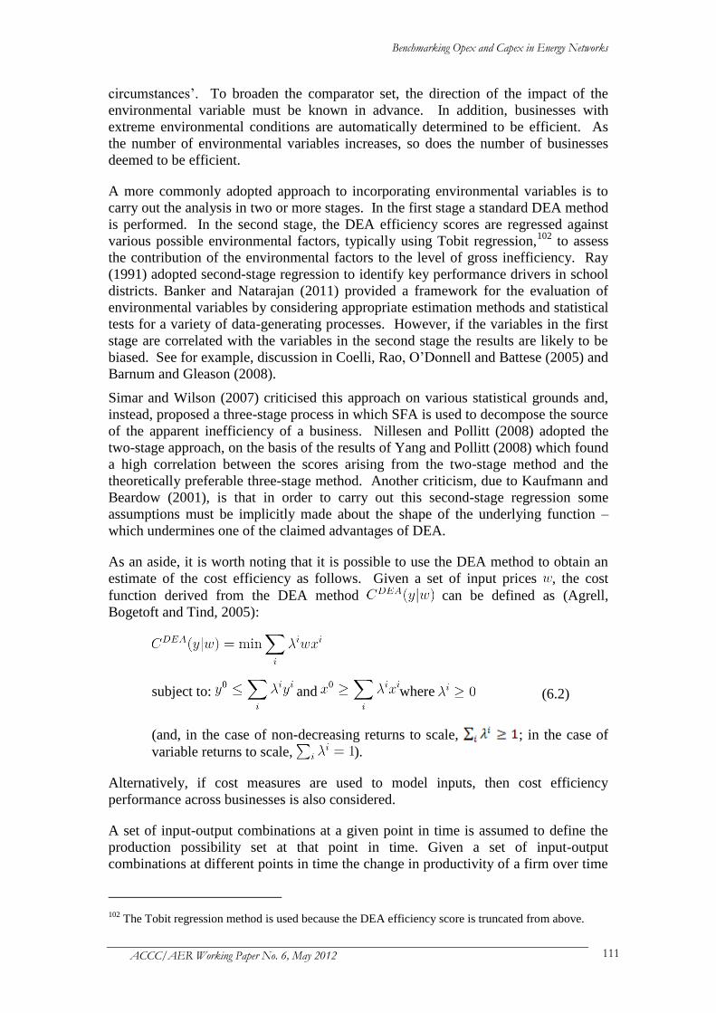
Benchmarking Opex and Capex in Energy Networks
ACCC/AER Working Paper No. 6, May 2012 111
circumstances’. To broaden the comparator set, the direction of the impact of the
environmental variable must be known in advance. In addition, businesses with
extreme environmental conditions are automatically determined to be efficient. As
the number of environmental variables increases, so does the number of businesses
deemed to be efficient.
A more commonly adopted approach to incorporating environmental variables is to
carry out the analysis in two or more stages. In the first stage a standard DEA method
is performed. In the second stage, the DEA efficiency scores are regressed against
various possible environmental factors, typically using Tobit regression,102
to assess
the contribution of the environmental factors to the level of gross inefficiency. Ray
(1991) adopted second-stage regression to identify key performance drivers in school
districts. Banker and Natarajan (2011) provided a framework for the evaluation of
environmental variables by considering appropriate estimation methods and statistical
tests for a variety of data-generating processes. However, if the variables in the first
stage are correlated with the variables in the second stage the results are likely to be
biased. See for example, discussion in Coelli, Rao, O’Donnell and Battese (2005) and
Barnum and Gleason (2008).
Simar and Wilson (2007) criticised this approach on various statistical grounds and,
instead, proposed a three-stage process in which SFA is used to decompose the source
of the apparent inefficiency of a business. Nillesen and Pollitt (2008) adopted the
two-stage approach, on the basis of the results of Yang and Pollitt (2008) which found
a high correlation between the scores arising from the two-stage method and the
theoretically preferable three-stage method. Another criticism, due to Kaufmann and
Beardow (2001), is that in order to carry out this second-stage regression some
assumptions must be implicitly made about the shape of the underlying function –
which undermines one of the claimed advantages of DEA.
As an aside, it is worth noting that it is possible to use the DEA method to obtain an
estimate of the cost efficiency as follows. Given a set of input prices , the cost
function derived from the DEA method can be defined as (Agrell,
Bogetoft and Tind, 2005):
subject to: and
where (6.2)
(and, in the case of non-decreasing returns to scale, ; in the case of
variable returns to scale, ).
Alternatively, if cost measures are used to model inputs, then cost efficiency
performance across businesses is also considered.
A set of input-output combinations at a given point in time is assumed to define the
production possibility set at that point in time. Given a set of input-output
combinations at different points in time the change in productivity of a firm over time
102
The Tobit regression method is used because the DEA efficiency score is truncated from above.
Benchmarking Opex and Capex in Energy Networks
ACCC/AER Working Paper No. 6, May 2012 112
can be computed. In principle, the business performances at time zero can be
computed using the production-possibility set from time one and vice versa. These
DEA scores can then be combined into a form of ‘Malmquist Index’ of productivity
change of the firm over time and its decomposition into efficiency change and
technical change. Coelli, Rao, O’Donnell and Battese (2005) provides a detailed
description of the computation of the Malmquist Index using DEA and SFA.
6.2.2 Data requirements
The standard approach to DEA focuses on the establishment of a production-
possibility set – the space of all feasible input-output combinations. As such, DEA
requires information on a set of input and output quantities. As noted above, if data
on input prices are also available or cost measures are used to model inputs, DEA can
be used to directly estimate a benchmark cost for each business.
As in all benchmarking methods, a key issue is the selection of the explanatory
variables – that is, the input, output, and environmental variables – which should, as a
group, be sufficient to model the production and thus the performance of the
businesses considered.
That is, the explanatory variables must account for all of the legitimate differences in
the cost performance of the businesses, including all the differences in cost that are
due to differences in the nature of the services provided, the customers served, the
quality of service provided, the weather conditions, operating environment, input
prices, and other factors that are out of management control.
The number of explanatory variables required to completely account for all of the
legitimate differences in the cost performance of businesses will differ from industry
to industry and study to study. Any variables which are common to all of the
businesses in the sample can be omitted from the analysis.103
Conversely the greater
the heterogeneity in the business conditions faced by the sample, the larger the
number of variables that will likely be necessary to account for that heterogeneity.
In modelling electricity distribution, the problems in relation to the selection of inputs
and outputs, as discussed in earlier chapters, are also relevant to the DEA method.
Ideally each distinct service provided should be treated as a different output and each
unique factor of production used should be separately modelled as an input.
However, as the number of inputs and outputs increases, the number of dimensions in
which the sampled businesses needed to compare with each other accelerates. A
general rule of thumb is that the sample size should be no less than, the product of the
number of inputs and number of outputs, or three times the sum of the number of
inputs and outputs, whichever is larger (Cooper, Seiford and Tone, 1999, p. 252).
Dyson, Allen, Camanho, Podinovski, Sarrico and Shale (2001) suggested a stricter
guideline requiring a sample size at least double the product of the number of inputs
and number of outputs. According to Coelli (2012), the information requirements for
DEA can be greater than SFA:
103
For example, this might apply to, say, national service standard obligations, nationally prevailing
weather conditions, or the prices of inputs with low transportation costs which are procured in a
national or international market.
Benchmarking Opex and Capex in Energy Networks
ACCC/AER Working Paper No. 6, May 2012 113
Given that DEA frontiers are arguably more flexible than a second-order parametric
frontier, such as the translog, one would expect that the data requirements for DEA are
greater than those of SFA. Hence, I believe that the existing rules of thumb used in the
DEA literature are generally too low. I would suggest that the construction of bootstrap
confidence intervals for DEA efficiency scores could provide some useful information
regarding the degree to which these DEA results obtained from small samples can be relied
upon.
As with other benchmarking methods, there is a need to use more aggregated input
and output measures under the DEA method.
Generally speaking, broad categories of outputs and inputs capable of capturing all
essential aspects of electricity distribution should be modelled. As discussed in
earlier chapters, there are a number of problems in measuring inputs and outputs for
electricity distribution, including that:
little consensus on which input-output variables best describe the production;
difficulties in modelling service quality;
problems with the aggregation of service capacity; and
difficulties with measuring the volume of capital input.
In addition, data are also required for modelling the set of environmental variables
needed for a two or three-stage DEA analysis.
6.2.3 Advantages and disadvantages
DEA is a relatively simple and intuitive technique.104
Its strength is that it requires
relatively little detailed knowledge of the shape of the underlying cost function. What
is required is the knowledge regarding (a) the key cost drivers – the factors that can
legitimately affect the volume of outputs produced from a given set of inputs and (b)
the basic shape of the technology (such as whether there are increasing returns to
scale). Unlike other benchmarking methods, DEA provides a clear picture of the
comparator business or business against which any given business is being compared.
Various possible disadvantages of DEA have been raised:
DEA neglects the possibility of errors in the measurement of the output and
input variables. As a result, the DEA measure is sensitive to the presence of
outliers or errors in the measurement of the data (see, for example, Pedraja-
Chaparro, Salinas-Jiménez, and Smith, 1999). In particular, the DEA efficiency
measure is sensitive to the input-output combinations for those (few) businesses
which define the boundary of the feasible space. Furthermore, adding more
104
Nillesen and Pollitt (2008, p. 20) emphasised that DEA is easy to communicate: ‘The great thing
about DEA is that it has a major advantage over other potential methodologies. It is easy to
communicate with managers. This is because it involves an engineering, rather than a statistical,
approach and all performance can be visually represented. Managers are in general much more
comfortable with direct estimates of efficiency and with fixed adjustments for potential, rather than
“letting the data decide” in an opaque way such as is the case with an econometric efficiency technique
such as Stochastic Frontier Analysis’.
Benchmarking Opex and Capex in Energy Networks
ACCC/AER Working Paper No. 6, May 2012 114
observations to the sample will result in a tendency for the DEA scores to
decrease.
DEA does not easily control for differences in business conditions. As
discussed in section 6.2.1, the alternative approaches to incorporating
environmental variables have their own problems. Kaufmann and Beardow
(2001) argued that the treatment of service quality is particularly difficult under
DEA.
Standard DEA allows for no internal validation of the model chosen, or whether
the resulting efficiency scores are statistically different from one. As Pedraja-
Chaparro, Salinas-Jiménez, and Smith (1999) emphasised:
The user of data envelopment analysis (DEA) has little guidance on model quality. The
technique offers none of the misspecification tests or goodness of fit statistics
developed for parametrical statistical methods. Yet, if a DEA model is to guide
managerial policy, the quality of the model is of crucial importance.
A related disadvantage is that it is not possible to know what sample size is
required to obtain a reasonable estimate of relative efficiencies.
Kaufmann and Beardow (2001) argued that a disadvantage of DEA was its use
of input volumes rather than input prices, given the difficulty in measuring the
volumes of capital services consumed.
Some of the disadvantages of DEA are addressed by recent developments in DEA,
including the development of statistical inference in DEA (Simar and Wilson, 1998,
1999, 2000; Kneip, Simar and Wilson, 2009), window analysis (see for example,
Webb 2003) and stochastic DEA. In a series of papers by Simar and Wilson, the
bootstrapping method has been applied to DEA modelling so that statistical inferences
can be made. In a recent paper Kuosmanen (2011) has further developed the
nonparametric DEA model by combining it with aspects of Stochastic Frontier
Analysis. Kuosmanen (2011) recommended replacing the use in Finland of an
average of DEA and SFA efficiency scores with the StoNED estimator, which
combines a nonparametric frontier with stochastic inefficiency and noise terms. The
resulting model was claimed to be a generalisation of both the classic DEA and SFA
models. The key idea is that the standard ‘least squares’ regression model is itself a
form of constrained-optimisation problem, similar to the classic problem. In
principle, a set of linear combinations of businesses which minimises the sum of the
squared deviation of the actual from the estimated costs can be found for a given set
of data on costs and outputs.
6.3 Literature review of the DEA method
The idea of measuring technical efficiency by a radial measure representing the
proportional input reduction possible while staying within the production possibility
set is due to Farrell (1957). The application of linear programming methods to
measuring technical efficiency under the CRS assumption (and the name Data
Envelopment Analysis) was first proposed by Charnes, Cooper and Rhodes (1978)
Benchmarking Opex and Capex in Energy Networks
ACCC/AER Working Paper No. 6, May 2012 115
and extended to the VRS model by Banker, Charnes and Cooper (1984).105
DEA is
also discussed in several surveys on productivity and efficiency measurement, such as
the article by Murillo-Zamorano (2004) or the textbook by Coelli, Rao, O’Donnell
and Battese (2005).
A number of academic papers have applied some form of DEA method to electricity
and gas distribution. Early contributions in this area were made by Charnes, Cooper,
Divine, Ruefli and Thomas (1989) and Miliotis (1992).
Charnes, Cooper, Divine, Ruefli and Thomas (1989) applied DEA to 75 Texas
electric cooperatives and compared the results to ratio and regression-based analyses
used for evaluating management efficiency. They considered DEA to be superior to
ratio analysis and decided to adopt DEA to assist the regulator to determine which
cooperatives might best be audited, provide reference businesses to judge the
performance of others and supply information as to source and magnitude of any
inefficiency that might be present.
Miliotis (1992) applied DEA to evaluate the relative efficiency of 45 electricity
distribution districts for the Greek Public Power Corporation. Miliotis (1992) used
eight input-output factors and considered four different DEA models, each with a
different combination of inputs and outputs. It was noted that, when using DEA,
inputs and outputs should be disaggregated up to a level where all the basic
idiosyncrasies of the system being modelled are represented, taking into account that
excessive breakdown of inputs and outputs may result in loss of discriminative power,
especially when the total number of businesses is relatively small. Miliotis (1992)
concluded that DEA scores appeared to be more reliable than simple productivity
ratios. The paper noted that the difference in DEA results between the businesses
might be due to the management of resources controllable by the business, the
efficiency of the design of the supply system or, finally, environmental aspects not
explicitly identified in the model.
Later development in this area covers DEA applications to a large number of
countries, such as Australia, the United Kingdom (UK), Finland, Norway, and
Switzerland. Table 6.1 summarises relevant empirical studies on energy networks in
terms of the sample, method, DEA model specification and assumptions.
Relatively few studies have taken into account quality of service measures when
carrying out DEA benchmarking. Among the few exceptions are Giannakis, Jamasb,
and Pollitt (2005) and Coelli, Crespo, Paszukiewicz, Perelman, Plagnet, and Romano
(2008). Giannakis, Jamasb, and Pollitt (2005) extended the DEA benchmarking of
electricity distribution businesses by including quality of service measures – indexes
of security of supply and reliability of supply – as an input variable. The authors
investigated the impact of the inclusion of quality of service measures as inputs into
the DEA model, and also the impact of including a measure of totex or opex. The
authors found that there were performance variations when quality of service
indicators were included in the model, which might indicate a possible trade-off
between the costs and quality of service.
105
A further problem is that there may be increasing returns to scale over some output levels and
decreasing returns to scale over others. Appa and Yue (1999) proposed a further extension to the basic
model to address this issue.
Benchmarking Opex and Capex in Energy Networks
ACCC/AER Working Paper No. 6, May 2012 116
Coelli, Crespo, Paszukiewicz, Perelman, Plagnet, and Romano (2008) used annual
data on 92 French electricity distribution businesses and included the total number of
interruptions as an input in the DEA model to account for quality of service.106
They
found that the inclusion of a quality variable had no significant effect upon mean
technical efficiency scores.
Several academic papers sought to assess whether or not DEA and other
benchmarking methods satisfy the consistency conditions proposed by Bauer, Berger,
Ferrier, and Humphrey (1998). Estache, Rossi and Ruzzier (2004) applied DEA and
SFA methods to 84 South American electricity distribution businesses and found a
high correlation in the efficiency ranking of utilities using CRS and VRS DEA
models, but a low correlation between SFA and DEA efficiency measures. Farsi and
Filippini (2005) applied DEA, SFA, and COLS methods to a sample of 59 Swiss
electricity distribution utilities.107
They found that although there was quite high
correlation between the COLS and SFA efficiency scores, the correlation with the
DEA estimates are relatively low. They concluded that the Bauer consistency
conditions were difficult to satisfy in the context of electricity distribution. Other
papers include Murillo-Zamorano and Vega-Cervera (2001), and Omrani, Azadeh,
Ghaderi, and Aabdollahzadeh (2010).
Several academic papers discussed the pros and cons of DEA (along with other
benchmarking methods). These include: Kaufmann and Beardow (2001), and
Ajodhia, Petrov and Scarsi (2003) in the context of the regulation of electricity
distribution; Burns, Jenkins and Riechmann (2005), and Lowry and Getachew
(2009b) in the context of public utility regulation more generally.
Kaufmann and Beardow (2001) evaluated alternative methods for benchmarking the
performance of power distributors, including DEA, SFA and econometric methods.
The authors considered that econometric techniques (such as econometric cost
functions and SFA) had significant advantages over DEA. The authors believed that
DEA was not well suited for electricity networks, particularly in countries like
Australia, where there are relatively limited data on domestic energy networks. The
authors considered a number of problems associated with implementing DEA for
energy networks, including problems with capital measurement, dealing with distance
and service quality, and the impact of non-comparable variables in international
datasets.
In another series of papers, Bogetoft (1997, 2000) set out a proposal for using DEA
mechanistically to determine the revenue allowance for a regulated business. This
proposal involves setting a revenue allowance for the regulated business which is a
weighted average of its past cost out-turns and a DEA score. Agrell, Bogetoft and
Tind (2005) applied this notion to the UK electricity distribution businesses.
106
Coelli, Crespo, Paszukiewicz, Perelman, Plagnet, and Romano (2008) expressed concerns with the
Giannakis, Jamasb, and Pollitt (2005) paper – specifically, the use of totex contains capex measures
‘which need not reflect the actual amount of capital services consumed in a particular year’ and the
small sample size problem. Coelli, Crespo, Paszukiewicz, Perelman, Plagnet, and Romano (2008) got
around these problems by applying DEA to a set of 92 electricity distribution businesses all operated
by EDF Réseau Distribution in France. See also Lassila, Honkapuro, Viljainen, Tahvanainen,
Partanen, Kivikko, Antila, Mäkinen and Järventausta (2005). 107
Discussion of Farsi and Filippini (2005) appears earlier in this paper at section 4.3.
Benchmarking Opex and Capex in Energy Networks
ACCC/AER Working Paper No. 6, May 2012 117
Bogetoft (1997) investigated the use of DEA in regulatory environments with
technological uncertainty. He found that regulatory schemes incorporating a
component of DEA estimated cost reductions would induce the regulated businesses
to minimise costs and minimise their information rents. Bogetoft noted many benefits
of DEA: it requires very little technical information; it allows a flexible, non-
parametric modelling of multi-input multi-output production process; and its cost
estimates are conservative or cautious because they are based on an inner
approximation of the production possibilities. Bogetoft (2000) similarly found that
the use of DEA could play a role in future planning and provide incentives to cost
minimisation.
Agrell, Bogetoft and Tind (2005) investigated the introduction of yardstick
competition in the Scandinavian countries and the use of DEA as a comparator. They
noted that using a DEA-based yardstick model compares favourably to the use of a
CPI–X model as it addresses issues relating to: the risk of excessive rents; the ratchet
effect; the arbitrariness of the parameters CPI and X; and the inability to
accommodate changes in the output profile. They noted that dynamic DEA yardstick
modelling is a potentially promising technique to address challenges facing a
regulator in a liberalised electricity market.
Overall, the academic literature on benchmarking using DEA urges a cautious
approach. Ajodhia, Petrov and Scarsi (2003, p. 270) considered that the main lesson
from the Dutch regulatory experience with DEA benchmarking is ‘perhaps that
regulators should take into account the limitations of benchmarking’. They further
argued for the use of benchmarking results as an informative tool rather than
mechanically to feed directly into the X factor. Lowry and Getachew (2009b)
suggested a number of improvements to make for using DEA as a regulatory
benchmarking tool. These include: the need to account for business conditions; and
the use of bootstrap method for statistical testing of DEA score. They considered that
benchmarking could either be used for prudence review in regulation or to aid in rate-
setting directly.
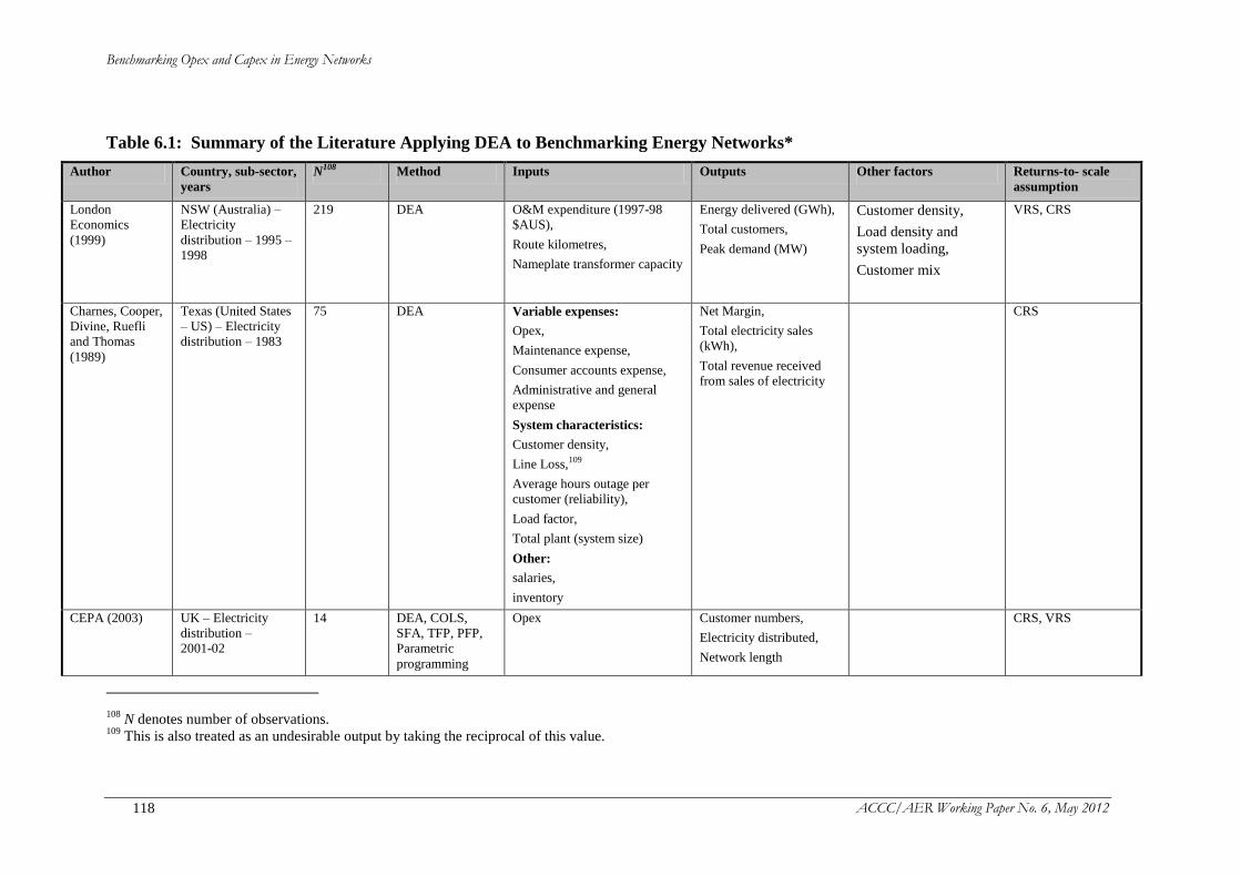
Benchmarking Opex and Capex in Energy Networks
ACCC/AER Working Paper No. 6, May 2012 118
Table 6.1: Summary of the Literature Applying DEA to Benchmarking Energy Networks*
Author Country, sub-sector,
years
N108 Method Inputs Outputs Other factors Returns-to- scale
assumption
London
Economics
(1999)
NSW (Australia) –
Electricity
distribution – 1995 –
1998
219 DEA O&M expenditure (1997-98
$AUS),
Route kilometres,
Nameplate transformer capacity
Energy delivered (GWh),
Total customers,
Peak demand (MW)
Customer density,
Load density and
system loading,
Customer mix
VRS, CRS
Charnes, Cooper,
Divine, Ruefli
and Thomas
(1989)
Texas (United States
– US) – Electricity
distribution – 1983
75 DEA Variable expenses:
Opex,
Maintenance expense,
Consumer accounts expense,
Administrative and general
expense
System characteristics:
Customer density,
Line Loss,109
Average hours outage per
customer (reliability),
Load factor,
Total plant (system size)
Other:
salaries,
inventory
Net Margin,
Total electricity sales
(kWh),
Total revenue received
from sales of electricity
CRS
CEPA (2003) UK – Electricity
distribution –
2001-02
14 DEA, COLS,
SFA, TFP, PFP,
Parametric
programming
Opex Customer numbers,
Electricity distributed,
Network length
CRS, VRS
108
N denotes number of observations. 109
This is also treated as an undesirable output by taking the reciprocal of this value.
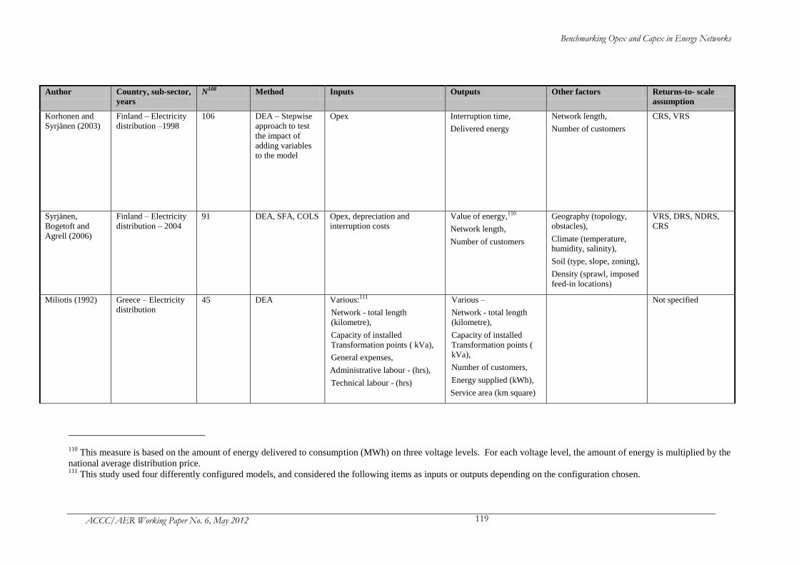
Benchmarking Opex and Capex in Energy Networks
ACCC/AER Working Paper No. 6, May 2012 119
Author Country, sub-sector,
years
N108 Method Inputs Outputs Other factors Returns-to- scale
assumption
Korhonen and
Syrjänen (2003)
Finland – Electricity
distribution –1998
106 DEA – Stepwise
approach to test
the impact of
adding variables
to the model
Opex Interruption time,
Delivered energy
Network length,
Number of customers
CRS, VRS
Syrjänen,
Bogetoft and
Agrell (2006)
Finland – Electricity
distribution – 2004
91 DEA, SFA, COLS Opex, depreciation and
interruption costs
Value of energy,110
Network length,
Number of customers
Geography (topology,
obstacles),
Climate (temperature,
humidity, salinity),
Soil (type, slope, zoning),
Density (sprawl, imposed
feed-in locations)
VRS, DRS, NDRS,
CRS
Miliotis (1992) Greece – Electricity
distribution
45 DEA Various:111
Network - total length
(kilometre),
Capacity of installed
Transformation points ( kVa),
General expenses,
Administrative labour - (hrs),
Technical labour - (hrs)
Various –
Network - total length
(kilometre),
Capacity of installed
Transformation points (
kVa),
Number of customers,
Energy supplied (kWh),
Service area (km square)
Not specified
110
This measure is based on the amount of energy delivered to consumption (MWh) on three voltage levels. For each voltage level, the amount of energy is multiplied by the
national average distribution price. 111
This study used four differently configured models, and considered the following items as inputs or outputs depending on the configuration chosen.
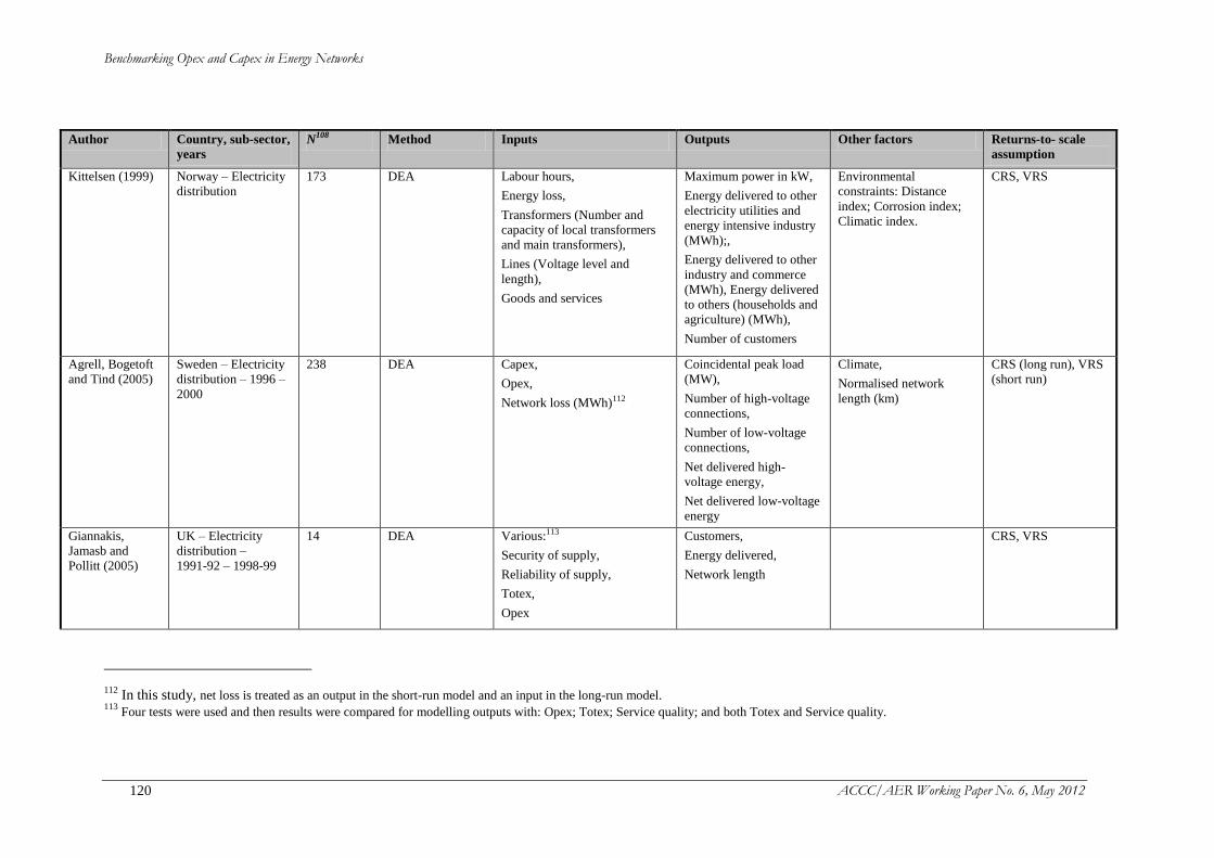
Benchmarking Opex and Capex in Energy Networks
ACCC/AER Working Paper No. 6, May 2012 120
Author Country, sub-sector,
years
N108 Method Inputs Outputs Other factors Returns-to- scale
assumption
Kittelsen (1999) Norway – Electricity
distribution
173 DEA Labour hours,
Energy loss,
Transformers (Number and
capacity of local transformers
and main transformers),
Lines (Voltage level and
length),
Goods and services
Maximum power in kW,
Energy delivered to other
electricity utilities and
energy intensive industry
(MWh);,
Energy delivered to other
industry and commerce
(MWh), Energy delivered
to others (households and
agriculture) (MWh),
Number of customers
Environmental
constraints: Distance
index; Corrosion index;
Climatic index.
CRS, VRS
Agrell, Bogetoft
and Tind (2005)
Sweden – Electricity
distribution – 1996 –
2000
238 DEA
Capex,
Opex,
Network loss (MWh)112
Coincidental peak load
(MW),
Number of high-voltage
connections,
Number of low-voltage
connections,
Net delivered high-
voltage energy,
Net delivered low-voltage
energy
Climate,
Normalised network
length (km)
CRS (long run), VRS
(short run)
Giannakis,
Jamasb and
Pollitt (2005)
UK – Electricity
distribution –
1991-92 – 1998-99
14 DEA Various:113
Security of supply,
Reliability of supply,
Totex,
Opex
Customers,
Energy delivered,
Network length
CRS, VRS
112
In this study, net loss is treated as an output in the short-run model and an input in the long-run model. 113
Four tests were used and then results were compared for modelling outputs with: Opex; Totex; Service quality; and both Totex and Service quality.
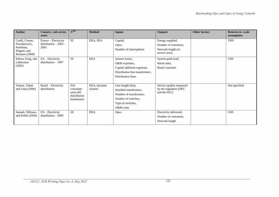
Benchmarking Opex and Capex in Energy Networks
ACCC/AER Working Paper No. 6, May 2012 121
Author Country, sub-sector,
years
N108 Method Inputs Outputs Other factors Returns-to- scale
assumption
Coelli, Crespo,
Paszukiewicz,
Perelman,
Plagnet, and
Romano (2008)
France – Electricity
distribution – 2003 –
2005
92 DEA, SFA Capital,
Opex,
Number of interruptions
Energy supplied,
Number of customers,
Network length (or
service area)
VRS
Pahwa, Feng, and
Lubkeman
(2002)
US – Electricity
distribution – 1997
50 DEA System losses,
O&M expenses,
Capital additions expenses,
Distribution line transformers,
Distribution lines
System peak load,
Retail sales,
Retail customer
CRS
Tanure, Tahan
and Lima (2006)
Brazil – Electricity
distribution
924
consumer
units (60
distribution
businesses)
DEA, dynamic
clusters
Line length (km),
Installed transformers,
Number of transformers,
Number of switches,
Type of switches,
O&M costs
Service quality measured
by the regulators (DEC
and the FEC)
Not specified
Jamasb, Nillesen,
and Pollitt (2004)
US – Electricity
distribution – 2000
28 DEA Opex Electricity delivered,
Number of customers,
Network length
CRS

Benchmarking Opex and Capex in Energy Networks
ACCC/AER Working Paper No. 6, May 2012 122
Author Country, sub-sector,
years
N108 Method Inputs Outputs Other factors Returns-to- scale
assumption
Agrell and
Bogetoft (2007)
Germany –
Electricity
distribution
328 DEA, SFA and
OLS analytic cost
model
Total direct cost (as specified in
the regulation) Service provision:
Number of meters,
Service area (by voltage –
high, medium, low)
Capacity provision:
Coincidental load (voltage
– high, medium, low
voltages; transformer –
HS/MS, MS/NS),
Feed-in power of
decentred generation
CRS, DRS, NDRS,
VRS
Wang, Ngan,
Engriwan and Lo
(2007)
Hong Kong –
Electricity
distribution – 1994 –
2003
2 DEA – Malmquist
TFP
Capex,
Labour
Electricity delivered,
Customer density
CRS
Cullmann and
von
Hirschhausen
(2007)
Germany, Poland, the
Czech Republic,
Slovakia and
Hungary – Electricity
distribution – 2002
84 DEA Number of employees,
Length of electricity grid
Total sales in GWh,
Number of customers.
Structural variable to
account for regional
differences:
Inverse Density Index
(IDI) – in km2 per
inhabitant
CRS
Carrington,
Coelli and
Groom (2002)
Australia and the US
– Gas distribution
59 DEA, PPI, OLS,
COLS, SFA
Length of distribution mains
(km),
O&M cost (covering labour,
contracting, network marketing,
etc.)
Total yearly deliveries (as
a proxy for capacity to
deliver gas),
Customer numbers (as a
proxy for connection
points) by residential and
other customers
Climate,
Age of network
VRS, CRS
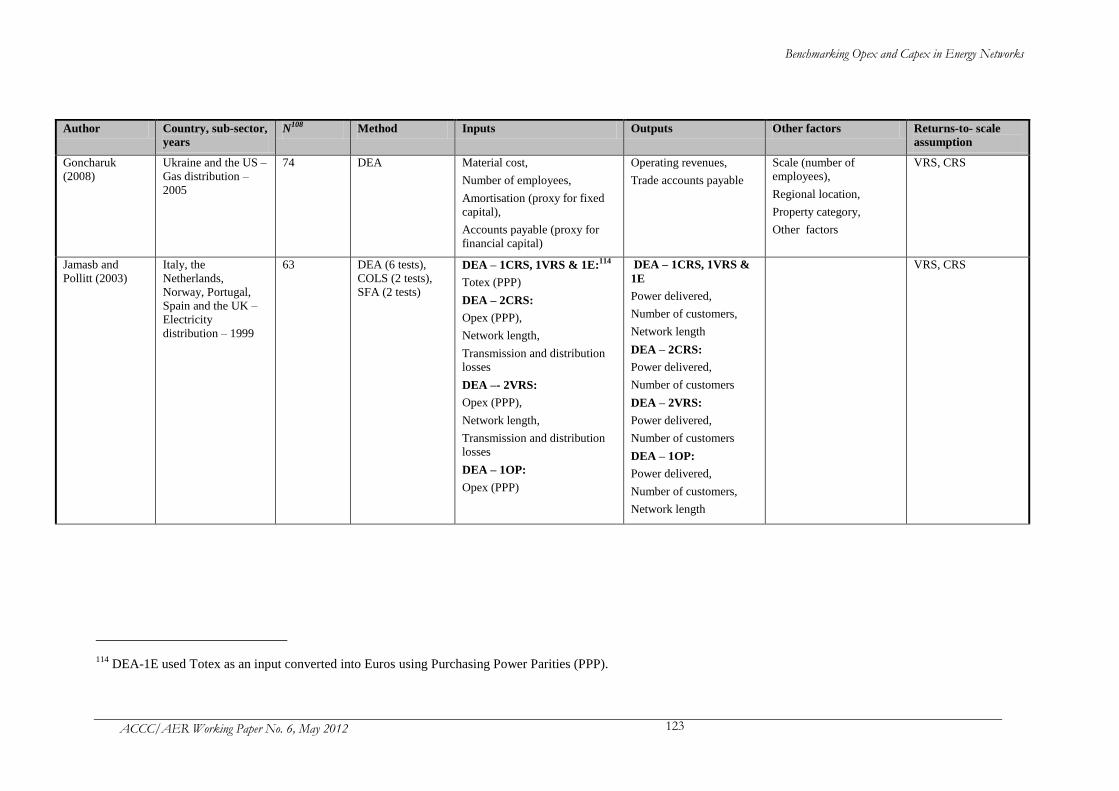
Benchmarking Opex and Capex in Energy Networks
ACCC/AER Working Paper No. 6, May 2012 123
Author Country, sub-sector,
years
N108 Method Inputs Outputs Other factors Returns-to- scale
assumption
Goncharuk
(2008)
Ukraine and the US –
Gas distribution –
2005
74 DEA Material cost,
Number of employees,
Amortisation (proxy for fixed
capital),
Accounts payable (proxy for
financial capital)
Operating revenues,
Trade accounts payable
Scale (number of
employees),
Regional location,
Property category,
Other factors
VRS, CRS
Jamasb and
Pollitt (2003)
Italy, the
Netherlands,
Norway, Portugal,
Spain and the UK –
Electricity
distribution – 1999
63 DEA (6 tests),
COLS (2 tests),
SFA (2 tests)
DEA – 1CRS, 1VRS & 1E:114
Totex (PPP)
DEA – 2CRS:
Opex (PPP),
Network length,
Transmission and distribution
losses
DEA –- 2VRS:
Opex (PPP),
Network length,
Transmission and distribution
losses
DEA – 1OP:
Opex (PPP)
DEA – 1CRS, 1VRS &
1E
Power delivered,
Number of customers,
Network length
DEA – 2CRS:
Power delivered,
Number of customers
DEA – 2VRS:
Power delivered,
Number of customers
DEA – 1OP:
Power delivered,
Number of customers,
Network length
VRS, CRS
114
DEA-1E used Totex as an input converted into Euros using Purchasing Power Parities (PPP).
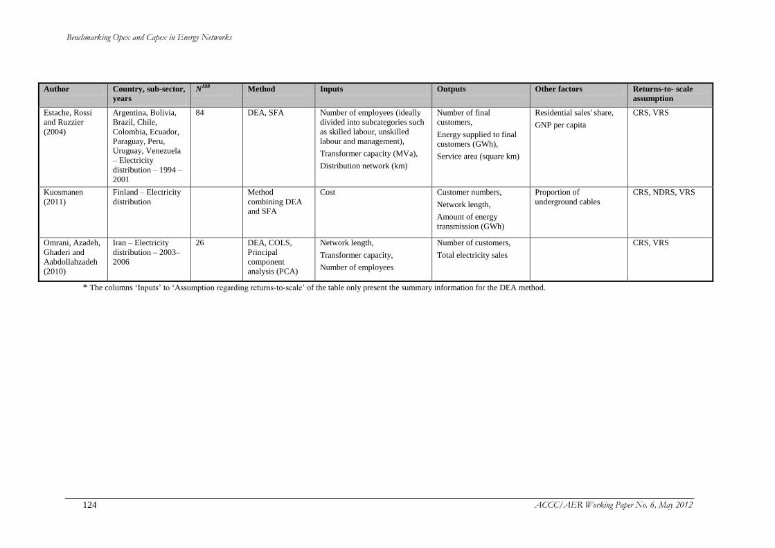
Benchmarking Opex and Capex in Energy Networks
ACCC/AER Working Paper No. 6, May 2012 124
Author Country, sub-sector,
years
N108 Method Inputs Outputs Other factors Returns-to- scale
assumption
Estache, Rossi
and Ruzzier
(2004)
Argentina, Bolivia,
Brazil, Chile,
Colombia, Ecuador,
Paraguay, Peru,
Uruguay, Venezuela
– Electricity
distribution – 1994 –
2001
84 DEA, SFA Number of employees (ideally
divided into subcategories such
as skilled labour, unskilled
labour and management),
Transformer capacity (MVa),
Distribution network (km)
Number of final
customers,
Energy supplied to final
customers (GWh),
Service area (square km)
Residential sales' share,
GNP per capita
CRS, VRS
Kuosmanen
(2011)
Finland – Electricity
distribution
Method
combining DEA
and SFA
Cost Customer numbers,
Network length,
Amount of energy
transmission (GWh)
Proportion of
underground cables
CRS, NDRS, VRS
Omrani, Azadeh,
Ghaderi and
Aabdollahzadeh
(2010)
Iran – Electricity
distribution – 2003–
2006
26 DEA, COLS,
Principal
component
analysis (PCA)
Network length,
Transformer capacity,
Number of employees
Number of customers,
Total electricity sales
CRS, VRS
* The columns ‘Inputs’ to ‘Assumption regarding returns-to-scale’ of the table only present the summary information for the DEA method.
Benchmarking Opex and Capex in Energy Networks
ACCC/AER Working Paper No. 6, May 2012 125
6.4 Regulatory practices using the DEA method
DEA benchmarking methods have been used by a number of energy regulators in the
determination of price and revenue requirements for electricity and gas distribution
businesses in countries, for example, Finland, Norway, the Netherlands, Germany,
and Austria; and in New South Wales, Australia.115
Haney and Pollitt (2009) also noted that,116
DEA had been considered in some form
by energy regulators in Belgium, the UK, Slovenia, Iceland, Norway, Argentina,
Brazil, Colombia, and Mexico. These countries are not reviewed here.
6.4.1 Regulatory practices review
Germany117
As discussed in section 5.4, the German regulator, the Federal Network Agency
(BNetzA) computed efficiency scores for the 198 electricity distribution businesses
and 187 gas distribution businesses under its jurisdiction using both DEA and SFA
benchmarking methods.
For electricity distribution both the DEA and SFA methods used totex as the input
variable (measured in two different ways). The output variables were: number of
connection points for high, medium and low-voltage levels, circuit of cables (high and
medium), circuit of lines (high and medium), network length (low), service area (low-
voltage level), annual peak load (high/medium and medium/low), number of
transformer stations across all three voltage levels, and installed capacity of
distributed generation across all thee voltage levels. The DEA model assumed
non-decreasing returns-to-scale (NDRS) technology.
Similarly, for gas distribution, the DEA and SFA methods, included totex as the input
variable and ten output variables: number of exit points to end-users, number of
potential exit points to end-users, service area, pipeline length (≤ 5 bars and > 5 bars),
annual peak load, potential peak load, volume of pipelines, population in 1995 and
population in 2006.
Finland118
The Finnish regulator (EMA) also used both DEA and SFA methods (as discussed in
section 5.4) to set the opex method which must be followed by 88 electricity
distribution businesses when they set their tariffs. The data used in the opex
benchmarking for the current regulatory period were taken from the average values
for the years 2003 to 2006. By using average values, the EMA hoped to smooth the
effects of random variation.
115
As it is not possible to cover all countries, there may be other examples of energy regulators
applying DEA benchmarking method that have not been captured in this paper and the supporting
research. 116
Haney and Pollitt (2009) undertook an international survey of benchmarking applications by 40
energy regulators. 117
Refer to chapter 3.4 of WIK-Consult (2011). 118
Refer to chapter 3.3 of WIK-Consult (2011).
Benchmarking Opex and Capex in Energy Networks
ACCC/AER Working Paper No. 6, May 2012 126
The DEA model used four variables – one input variable and three output variables.
The input variable was the overall costs to customers, composed of the sum of total of
controllable operational costs, depreciation and outage costs. The output factors were
total length of the electricity network, number of users of the network operator and the
value of energy distributed for consumption. The EMA adopted an input-oriented
version of the DEA model under NDRS.
The efficiency score results of the SFA and DEA methods were combined by taking a
simple average, which provides the efficiency target for the business to reduce costs
to achieve an efficient cost level under the prescribed opex method.119
Austria120
As discussed in section 4.4, the Austrian energy regulator (E-control) used an
incentive-based approach to set the revenue allowances for electricity and gas
distribution businesses in 2006 and 2008 respectively. The E-control used
benchmarking methods to set a business-specific X factor which is deducted from the
price cap. The X factor is the sum of a generic X factor for the industry and an
amount proportional to the degree of business-specific inefficiency.121
Inefficient
distribution businesses were, in effect, provided with lower rates of increase in real
revenues.
The E-control used both DEA and MOLS benchmarking methods to assess the
relative efficiency of each distribution business. The decision to aggregate the results
of the three benchmarking models and the decision on the weightings were based on
compromise with the industry (WIK-Consult, 2011).
Electricity distribution
For electricity distribution, total expenditure (totex) was the sole input variable,
(which was the sum of opex, excluding the costs for the usage of upstream networks,
plus capex). Two DEA models were estimated with different combinations of output
variables; both models assumed CRS. The E-control also estimated a MOLS model
which is described in section 4.4. The output variables for the models were chosen
based on analysis of an engineering-based reference model.
The first DEA model – DEA(I) - had three output variables: peak load of the medium
voltage level (PMV), peak load of the low voltage grid (PLV), and an aggregate network
length variable (lT)calculated as a weighted sum of network lengths at the three
voltage levels:
LVMVHVT llll 66.183.5 (6.3)
The second DEA model – DEA(II) – used five output variables: the two peak load
variables (PMV, PLV) and the three network length variables (lHV, lMV, lLV) separately.
119
The use of averages of efficiency scores derived has been criticised by Pollitt (2005). 120
Refer to chapter 3.1 of WIK-Consult (2011). 121
The formula for the X factor is provided in section 4.4.
Benchmarking Opex and Capex in Energy Networks
ACCC/AER Working Paper No. 6, May 2012 127
With only 20 observations, the E-control considered that DEA(II) (with six variables)
was not able to fully discriminate between the efficiency performances of different
businesses. The final business-specific efficiency score was a weighted average of the
two DEA scores and the MOLS score, with less weight applied to the DEA(II) model.
Gas distribution
The E-control used a similar approach for the gas distribution sub-sector. Two DEA
and two MOLS models were estimated. The DEA models assumed CRS with a 75
per cent limit on the maximum input/output contribution. The input variable was
based on total costs including opex and capex. For the first model capex was
measured as index historic costs and for the second model, capex was based on
annuity. The output variables were the same for both models; these were: weighted
network length, peak load of industrial customers, and metering points for residential
customers. Each model was estimated by DEA and MOLS, resulting in four sets of
efficiency results.
The E-control took an average of the two DEA models to give a DEA efficiency score
and did the same for the MOLS models. The final efficiency score for each gas
business was a weighted average, with 60 per cent given to the higher score, DEA or
MOLS, and 40 per cent to the other.
Norway122
With 150 electricity distribution businesses, Norway was one of the first European
countries to introduce incentive regulation based on efficiency benchmarking. For the
most recent regulatory period, 2007 to 2012, the Norwegian Water Resources and
Energy Directorate (NVE) set a revenue allowance which was a weighted average of
the out-turn cost (weight = 0.4) and a benchmark cost determined through a DEA
analysis (weight = 0.6). The data for both the out-turn costs and the DEA model were
from two years prior to the start of the five-year regulatory period.
The DEA model used a single input, six outputs, various environmental variables and
assumed CRS. The input variable was total costs covering operating costs, capital
costs, and quality costs (measured by the value of lost load). The output variables
were energy delivered, customers, cottage (small) customers, high voltage lines,
network stations (transformers), and interface.123
Environmental variables included
measures of snow, forest, and coastal climate.
The model used by the NVE was for super-efficiency score analysis,124
such that the
scores may be higher than 100 per cent. The DEA efficiency estimates were
calibrated such that the cost-weighted-average efficiency score was 100 per cent.
This implied that a representative utility, with an average efficiency score, is allowed
to earn the normal rate of return, and an efficient utility can earn more than the normal
rate of return.
122
Refer to chapter 3.5 of WIK-Consult (2011). 123
The interface variable is the cost weighted sum of equipment in the interface between distribution
and transmission networks. 124
This method is first proposed by Andersen and Petersen (1993) and has often been used to provide a
ranking system that allows for comparison of efficient businesses.
Benchmarking Opex and Capex in Energy Networks
ACCC/AER Working Paper No. 6, May 2012 128
Since 2009, the NVE’s efficiency benchmarking model has also controlled for factors
influencing the efficiency level rather than the production technology. The
amendment involved correcting the DEA scores ex post through regression analysis.
The regression analysis aimed to estimate the efficiency effect of the number of
connections to regional networks, installed capacity for small hydro power generators
connected to the grid and the number of remote islands supplied.
The Netherlands125
When incentive regulation was introduced in the Netherlands from 2001, the energy
regulator, DTe, employed DEA benchmarking methods to assess the relative
efficiency of around 20 electricity distribution businesses.126
It was intended that the
DEA efficiency scores would form one aspect of X factor, which also included an
estimate of industry-wide general efficiency change (refer to section 2.4). The
relative efficiency scores would only be included for the first two regulatory periods
to provide up to six years for inefficient distribution businesses to ‘catch-up’ with
efficient businesses.
Using data based on 20 local electricity distribution businesses in 1999,127
the DEA
model employed by the DTe included:128
Total controllable costs (opex, depreciation and standardised capital costs) as the
input variable;
Energy delivered, number of large customers, number of small customers, peak
demand at distribution level, and peak demand at transmission level as the
output variables; and
Number of transformers and network route length as the environmental
variables.
Efficient businesses were assigned a DEA score of one and inefficient businesses a
DEA score of less than one. The business-specific DEA score was then multiplied by
the actual costs of the business to derive efficient costs in the base year (i.e., 2000).
In the first regulatory period (2001 to 2003), however, the DTe’s inclusion of the
relative efficiency component in the X factor was overturned in subsequent litigation
and only the industry-wide general efficiency component of the X factor remained.
As a result, the DTe sought a legislative change to allow the inclusion of the
individual efficiency component in the second regulatory period (2004 to 2006).
125
Refer to chapter five of ‘Regulatory Practices in Other Countries’ (ACCC/AER, 2012). 126
It was the DTe’s consultants, Frontier Economics, who recommended the use of DEA rather than
econometric methods on the basis of the small sample size. 127
The initial analysis by Frontier Economics included data on both electricity distribution and supply
businesses in 1996. Frontier Economics intended to separate out the 20 distribution businesses from
supply businesses and update the analysis for 1999 data. As the final report is not publicly available,
secondary sources of information are used in this paper to confirm the use of 20 distribution businesses
but not the time period. 128
It is unknown which returns-to-scale assumption was employed by the DTe.
Benchmarking Opex and Capex in Energy Networks
ACCC/AER Working Paper No. 6, May 2012 129
Australia
In 1999, the Independent Pricing and Regulatory Tribunal of NSW (IPART) reviewed
the relative efficiency of NSW Australian electricity and gas distribution businesses
against other Australian and international distribution businesses. The IPART used a
building-block model to determine allowable revenues for each regulated business
and the results of the cost benchmarking analysis were used to inform the assessment
of their efficient costs.
Electricity distribution
London Economics (1999) was commissioned to report on the efficiency of NSW
electricity distribution businesses. DEA was used to benchmark the NSW utilities
against Australian and international utilities. The sample included 219 electricity
distributors from Australia, England, Wales, New Zealand and the United States (US),
with the sample periods slightly different for each country.
The inputs used in the DEA model were total O&M expenditure (in 1997-98 $AUS),
route kilometres and nameplate transformer capacity. Outputs were total energy
delivered (in GWh), total customers and peak demand (in MW). VRS was assumed.
A second-stage Tobit regression was employed to adjust the gross DEA efficiency
scores to account for environmental differences.
Various other benchmarking methods were used for sensitivity analysis including
Tornqvist TFP and SFA. IPART (1999) considered that the deviation between the
results was expected due to the known characteristics of the different methods.
Gas Distribution
Following the London Economics (1999) study, IPART (1999) conducted its own
efficiency benchmarking of seven Australian gas distribution businesses against 51
gas distribution businesses in the US using similar methods.
IPART (1999) estimated a DEA model with the VRS assumption. The input variables
were O&M costs and capital costs (measured by the length of distribution mains).
The output variables considered were the amount of gas delivered (TJ), the number of
residential customers and the number of other customers. Environmental factors
considered were climate and age of the network. Two methods of incorporating these
were explored, the first of which was the direct inclusion of environmental factors
into the DEA model and the second method used a second-stage Tobit regression.
These are ultimately found to have minimal impact on the results.
Sensitivity analysis was conducted on the results using an alternative DEA model
specification incorporating quality of services, and the COLS and SFA methods. The
alternative DEA model used the same inputs but considered the amount of gas
delivered, the total number of customers and the reciprocal of unaccounted-for gas for
the outputs.
Benchmarking Opex and Capex in Energy Networks
ACCC/AER Working Paper No. 6, May 2012 130
6.4.2 Summary of regulatory practices
DEA benchmarking methods have been applied by a number of the European
regulators. DEA has also been applied in the Australian context by combining the
data on Australian distribution businesses with comparable international distribution
businesses to increase the sample size.
Austria, Germany and Finland all combined the efficiency scores from the DEA
method with the efficiency scores derived from alternative methods such as modified
ordinary least squares and SFA. Both London Economics (1999) and IPART (1999)
undertook extensive comparisons of the results of DEA models against the results of
COLS and SFA methods. The Dutch and Norwegian regulators, however, only
considered the result from DEA analysis. In the Netherlands, a sample size of 20
distribution businesses was considered to be insufficient to confidently employ
econometric methods.
With data on 198 electricity and 187 gas distribution businesses, the German regulator
was able to include a large number of dependent variables in the DEA model, 11 and
ten for electricity and gas respectively. Similarly, the Norwegian regulator with 150
electricity distribution businesses included nine variables. The Austrian and
Netherlands regulators, with only 20 distribution businesses in their samples, included
fewer variables in the model.
6.5 Issues arising from the review
The above sections review the use of the DEA method for efficiency analysis of
energy utilities in a sub-sector. The review covers the theoretical foundation of DEA,
empirical applications by researchers, mostly in the context of the energy sector, and
regulatory applications by sectoral regulators.
A number of issues seem to arise in the application of DEA to benchmarking
electricity and gas networks. The choice of variables, the model specification and the
size of the sample are critical factors in determining how much weight can be put on
the DEA results.
6.5.1 The choice of variables
As already emphasised, the selection of the input and output variables is of critical
importance.129
Unfortunately there is no consensus on how these variables should be
chosen.
As shown in Jamasb and Pollitt (2001) and noted by Giannakis, Jamasb and Pollitt
(2005), choosing the input-output specification is an important step in DEA, but the
literature has shown a lack of consensus on which variables best describe the
operation of electricity distribution utilities. Burns, Jenkins and Riechmann (2005)
instead considered that the range of models largely reflected the particular research
questions to answer. For example, the model specifications can differ depending on
whether the short-term performance or long-term performance is modeled. They
129
Note that much of the discussion on the choice of variables is also applicable to other benchmarking
methods reviewed in this paper.
Benchmarking Opex and Capex in Energy Networks
ACCC/AER Working Paper No. 6, May 2012 131
recommended a systematic approach for variable specification involving both
theoretical analysis (e.g., model network analysis, intuition and heuristics) and
empirical analysis (e.g., regression analysis).
Coelli, Crepo, Paszukiewicz, Perelman, Plagnet, and Romano (2008) provided some
justifications for its chosen three-output and three-input model specification in their
DEA study of French electricity distribution businesses. They followed the literature
of electricity distribution benchmarking to model standard output characteristics, such
as energy supplied (in MWh), number of customers and network size (e.g., service
area or network length), but specifically incorporated a quality measure as an input to
examine the impact of modelling quality of services on efficiency benchmarking.
They highlighted the difficulties in selecting just a few variables for accurately
capturing all of the relevant differences in inputs and outputs. Instead, their study
focussed on capturing the key aspects of output heterogeneity and input variations.
Specific issues arise with respect to individual choices of variables: For example,
while the number of customers is usually considered as an output, should the network
length (in kilometre) be considered an input or an output? In one view, poles and
wires are capital inputs into the final service (delivery of electricity to the location of
the customer) and therefore should be treated as inputs. In another view, length of
network showing the scope of operation can be used as a proxy for customer density –
a legitimate driver of costs. However, viewing network length as an output runs the
risk that a network that increases its length of lines is rewarded even if there is no
impact on the real-world delivery of service to customers. In their survey of 20
benchmarking studies of energy network, Jamasb and Pollitt (2001) reported that size
was treated as an input in 11 studies and as an output in four other studies. Jamasb,
Nillesen and Pollitt (2004, p. 830) commented that ‘in extremis certain variables may
be used as inputs in one regulatory model, whereas in other regimes they are used as
outputs’.
Another issue concerns the use of the ‘quantity of electricity delivered’ (usually
measured in GWh). The use of this throughput measure is quite common in DEA
studies of electricity distribution as it is often considered as the only homogeneous
product of the electricity distribution (Kittelsen, 1999, p. 16). According to Jamasb,
Nillesen and Pollitt (2004), Allas and Leslie (2001) reported that about 85 per cent of
costs varied with the number of customers and the units of energy delivered.
However, Turvey (2006) criticised the use of volume of electricity delivered as an
output and argued for the use of a capacity measure:
The throughput of a network of pipes and wires … is not determined by the enterprise and
should not be regarded as its output. … What the enterprise provides is not gas,
electricity, water or messages; it is the capacity to convey them. It follows that, to
compare efficiencies, it is necessary to compare differences in capacities with differences
in costs.
Another concern relates to the specification of inputs. Most studies recognise the
difficulty of measuring the supply of services from capital assets. In practice this is
reflected in the arbitrariness of the choice of the allocation of capital costs into a
single period.130
Many benchmarking studies simply chose to exclude consideration
130
Turvey (2006) went into some detail on the measurement of capital services using what was
described as ‘heroic assumptions’.
Benchmarking Opex and Capex in Energy Networks
ACCC/AER Working Paper No. 6, May 2012 132
of capital costs and focus entirely on operating and maintenance expenditures.
Unfortunately, an exclusive focus on operating costs ignores the possibility of trade-
offs between capital and operating expenditure and will not identify the most efficient
firm from the total cost perspective. In addition, benchmarking studies which ignore
capital expenditure will tend to favour businesses with young assets, even when that
asset replacement decision is socially inefficient overall.131
Another issue relates to the difficulty of measuring the quality of labour inputs. Even
where data are available on number of hours worked, different workers and different
types of workers presumably provide different services. A common solution to this
problem is to value all inputs at their cost, and to use an aggregated input cost
measure in the benchmarking. A difficulty with this approach is that labour input
price can vary across businesses. Using this cost measure as an input, a business in a
high labour-price location would appear less productive than a business in a low
labour-price location for no fault of its own.132
In this case, (labour) price deflators at
the regional level, if available, need to be used to deflate the labour cost.
Issues also arise in choosing the total number of input and output variables. DEA
may find many of the sampled businesses efficient where the number of input-output
variables (or operating condition variables) is large relative to the size of the sample,
(Coelli, Rao and Battese, 1998, p. 181). Burns, Jenkins and Riechmann (2005) noted
the lack of an ability to discriminate between businesses by DEA relative to
econometric analysis. However, they emphasised that the solution was not to reduce
the number of input-output variables which might result in mis-specification or under-
specification of the benchmarking model.
Increasing the number of input-output variables will tend to capture more dimensions
of input and output combination that firms can be compared with each other and will
also tend to make more firms appear on the frontier. As pointed out by Kittelsen
(1999), non-parametric DEA methods have problems with collinearity or irrelevant
variables. In fact, the inclusion of a purely irrelevant factor (such as a random
number) will still make some businesses appear to be efficient. Kittelsen (1999) went
on to suggest stepwise DEA that uses statistical tests to evaluate sensitivity of
efficiency results with respect to variable disaggregation and addition and to assist the
determination of model specification.
It might be argued that a possible solution to input-output specification is through
testing of a number of alternative model specifications, with different input, output
and environmental variables. However as noted earlier, DEA offers no internal
mechanism for validating the selection of particular variables. The use of bootstrap
methods for statistical testing of DEA efficiency scores may offer some useful
information regarding the degree to which DEA results obtained from small samples
can be relied upon.
131
This assumes that the operating and maintenance expenditures per transformer or per kilometre of
line depend, in part, on the age of the underlying assets. 132
Another issue relates to the treatment of network losses. Very few benchmarking studies of
distribution businesses include losses at all, but network losses are, in principle, controllable by the
distribution business in the long run.
Benchmarking Opex and Capex in Energy Networks
ACCC/AER Working Paper No. 6, May 2012 133
6.5.2 The specification of the DEA model
In any application of the DEA method, decisions must be made as to the construction
of the set of feasible input-output combinations. This involves the consideration of
two issues: input- or output-orientation and the nature of returns-to-scale.
The choice of input-orientation and output-orientation model depends on whether the
business has most control over the inputs or the outputs. If the business is considered
as having greater control over input quantities relative output quantities, then an input-
oriented model with input-reduction focus should be used. Conversely, if the business
is considered to have greater control over output quantities, then an output-oriented
model with output-expansion focus should be used. For the regulated electricity
distribution utilities, the outputs are generally assumed to be exogenously given. An
input-oriented model is therefore generally used. By definition, the orientation
assumption has no impact on the efficiency results only under a CRS model.
Empirically the choice of orientation may only have a minor impact upon the
efficiency scores estimated (see for example, Coelli and Perelman, 1999).
The most common approach to DEA assumes that feasible input-output combinations
can be scaled and combined without constraint. This excludes the possibility of
alternative assumptions to CRS technology. This assumption can be weakened but
doing so may weaken the ability of the DEA model to discriminate between
businesses. For example, the variable returns-to-scale (VRS) model effectively
compares a business only with businesses of a similar size rather than all sampled
businesses regardless of their size.
The choice of constant or variable returns-to-scale model may, in part, depend on the
nature of returns-to-scale in the industry. Jamasb, Nillesen and Pollitt (2004, p. 834)
noted that there had been empirical evidence of the presence of economies of scale in
electricity distribution networks. They cited a number of studies on Switzerland,
Norway, New Zealand and Canada, which estimated the minimum efficient firm size
to be around 20 000 to 30 000 customers. However, in practice CRS is more
commonly assumed. Both the Dutch and Norwegian regulators have used CRS DEA
models by assuming that electricity distribution utilities can freely adjust their scale of
operations through mergers and acquisitions. In contrast, the UK regulator has
consistently applied VRS DEA by taking the number and the size of electricity
businesses in the industry as given. The German and Finnish regulators have assumed
NDRS in their DEA models, under which small networks were only compared with
other small networks. This would penalise too large networks operating at sub-
optimal scale in the short-run. The choice may also affect the long-term structure of
the industry.
6.5.3 Importance of data quality
As a deterministic technique that has no account for measurement errors, DEA is
particularly sensitive to outlying observations (i.e., observations with usually large or
small values). Therefore, there is a strong need to screen for potential outliers when
assembling the data used for DEA analysis. Necessary steps of assessments include:
Use descriptive statistics (including tabular and graphical analysis) to identify
outlying observations for further checking.

Benchmarking Opex and Capex in Energy Networks
ACCC/AER Working Paper No. 6, May 2012 134
Correcting outlying observations if they are found to have been incorrectly
entered.
Use super-efficiency DEA or other modified DEA, under which certain
observations (including the business under evaluation and/or outlying
observations identified) can be excluded from form the reference production set.
The super-efficiency DEA was first proposed by Andersen and Petersen (1993)
to provide a ranking for efficient businesses.
A related problem in regulatory applications has been identified by Jamasb, Nillesen
and Pollitt (2004). According to their paper, since the DEA measure depends strongly
on the input-output combinations of a few boundary businesses, there can arise scope
for strategic action taken by regulated utilities to manipulate the location of the
boundary through, for example, mergers, or collusion in the reporting of results.
Their analysis of the US utility data suggested that strategic behaviours by regulated
businesses could have significant effects on the measured firm performance and
profitability. They considered that the regulators should note the importance of
ensuring reliability of regulatory data and conducting sensitivity analysis with respect
to method and model specification.
6.5.4 Validation of a DEA model
As already noted, one of the key drawbacks of the DEA method is that it is impossible
to interpret the validity of the results within the framework of the model itself.133
Unlike econometric methods, DEA does not offer diagnostic statistics to test for the
possibility of model misspecification or to assess the overall goodness of fit of the
model. Pedraja-Chaparro, Salinas-Jiménez and Smith (1999) noted that a DEA model
might offer misleading results as a result of model mis-specifications (due to incorrect
variable inclusions or exclusions and an incorrect returns-to-scale assumption) and/or
inadequate data. In their views, the performance of a DEA model depends on
amongst other things, the distribution of efficiencies, the number of factors included
in the analysis, the size of the sample, and the degree of correlation between factors.
They emphasised that whether a DEA model specification is adequate depends on the
research question to answer. Based on their simulation study, they rejected the use
of simple rules of thumb (e.g., number of inputs and outputs relative to sample size) to
guide on the reliability of the results obtained.
One way to validate the model specification and results is to examine the DEA peers
of each business to see if the model is producing sensible benchmarks (i.e.,
comparator businesses).
Most importantly, the validation of a DEA model should come from external sources
– that is, from a careful independent assessment of the necessary variables and cost
drivers, together with a careful choice of the assumptions underlying the DEA
method. The need to use economic theory and industry knowledge to choose model
specification should not be forgotten when some specification issues can be driven by
133
CEPA (2003, pp. 64-65) stated that: ‘One of the key drawbacks of the DEA methodology is that it is
difficult to assess the significance of the results ... Overall we believe that DEA is a theoretically
appealing benchmarking technique that is easy and practical to implement ... However it cannot be
relied upon in isolation due to the difficulty in assessing the significance of the results obtained.’

Benchmarking Opex and Capex in Energy Networks
ACCC/AER Working Paper No. 6, May 2012 135
data. These choices may also be informed by careful engineering industry studies.
Finally, as large a dataset as possible must be compiled.
6.6 Conclusions
DEA is a straightforward technique that uses observations of feasible input-output
combinations to create a set of feasible input-output combinations against which the
performance of other businesses can be assessed. The basis for an efficiency score for
any individual business can be reasonably easily communicated. It is particularly
useful where there are a large number of comparable businesses producing essentially
homogeneous outputs.
The validity of any particular application of DEA rests on the assumptions made –
that is, the choice of the input, output and environmental variables and the returns to
scale assumptions. It is therefore important that any application of DEA carefully
considers and justifies the use of a particular set of variables. It is also important that
the largest possible data sample be used – including distribution businesses in other
countries if necessary.
For a DEA benchmarking study to have a degree of authority, four steps should be
carefully followed: First, the input, output, and environmental variables should be
carefully chosen to capture all of the important aspects of operations run by electricity
distribution utilities. This should normally be based on sound economic theory and
industry knowledge and probably be carried out using careful engineering analysis.
Second, the basic features of the underlying production function need to be
determined – such as the presence of economies of scale and the ability of individual
businesses to scale up or down the activities of other businesses. Third, as large a
dataset as possible needs to be compiled – while it is not possible to know what
sample size is required to obtain a reasonable estimate of relative efficiencies, larger
sample size relative to the number of input-output dimensions modelled would
increase the discriminatory power of a DEA model. Finally, the DEA benchmarking
should generally be an iterative, collaborative process with industry participants
(regulated businesses and customers), which allows for progressive improvement in
the model specification and the enumeration of the factors necessary to differentiate
different firms.
A credible DEA study is likely to shed some light on the shape of the cost function
underlying distribution businesses and may shed some light on key cost drivers and
the rate of technological change. At least, DEA may play a role in identifying a
particular group of actual observations, which, in combination, produce more
efficiently than a business under evaluation. This information could possibly be used
as the basis for further investigation aimed at identifying business best practices
which should be and could be copied by other businesses in the industry.

Benchmarking Opex and Capex in Energy Networks
ACCC/AER Working Paper No. 6, May 2012 136
Chapter 7 Common issues in benchmarking of energy networks
7.1 Introduction
Benchmarking of energy networks, particularly those operating in electricity
distribution, has been conducted in both academic literature and regulatory practices.
As surveyed by Jamasb and Pollitt (2001) and Haney and Pollitt (2009), a variety of
benchmarking methods have been used by energy regulators across the countries and
jurisdictions reviewed, with a notable preference for the non-parametric methods.
There are a number of technical issues for benchmarking. Researchers and regulators
often consider that benchmarking should be used with caution and its limitations
should be recognised; for example, Ajodhia, Petrov and Scarsi (2003), Shuttleworth
(2005), and Farsi and Fillipini (2004).
Based on the review of alternative benchmarking methods in chapters 2 to 6, this
chapter summarises major technical issues in benchmarking of energy networks, such
as data and model-specification issues. The following chapter will consider
regulatory challenges in applying benchmarking.
The rest of the chapter is structured as follows. Section 7.2 provides a summary of
the review of alternative benchmarking methods. Potential data issues and model-
specification issues are discussed in sections 7.3 and 7.4 respectively. Section 7.5
provides some insights into benchmarking of energy networks before drawing
conclusions in section 7.6.
7.2 Summary of alternative benchmarking methods
The foregoing review of alternative benchmarking methods, namely partial
performance indicators (PPI), index-number-based Total Factor Productivity analysis
(TFP), econometric method (EM), Data Envelopment Analysis (DEA), Stochastic
Frontier Analysis (SFA), examines method, model and data requirements, as well as
advantages and disadvantages relative to each other.
There is no clear consensus in the literature in relation to which benchmarking
approach should be used by economic regulators. As identified previously, each
method has relative strengths and weaknesses.
Table 7.1 below summarises key characteristics of the five benchmarking methods
reviewed.
The advantage of PPI and index-based TFP methods is their relatively simple
theoretical basis and their relative ease of calculation. Unlike EM, SFA and DEA, the
PPI and TFP methods do not involve the estimation of an underlying cost or
production technology of the industry.
PPI has been used by Australian energy regulators, including the AER. In the
regulatory context, TFP has been used, or at least considered, for determinations of an
X factor, or its frontier-shift component in: the Northern Territory (Australia), New
Zealand, Canada, the Netherlands and Austria.
However, the relative theoretical simplicity of the PPI and TFP methods is also a
weakness. PPI may fail to properly model a multiple-input and multiple-output
Benchmarking Opex and Capex in Energy Networks
ACCC/AER Working Paper No. 6, May 2012 137
production process because the partial approach to performance measurement can be
too simplistic. That is, the PPI may not be capable of modelling the overall
performance of the business or the industry. The TFP method has a rigorous
grounding in economic theory. However, the TFP is relatively information intensive
as it requires price and quantity data for both input variables and output variables.
The parametric approaches, EM and SFA, require the estimation of a specific
functional form that is sufficiently flexible to capture the structure of the underlying
production process. The problem is that estimation of a functional form that is not
sufficiently flexible will result in biased results.
A strength of EM and SFA, from an economic perspective, is their relatively strong
theoretical basis. EM and SFA use economic theory to attempt to capture the
industry’s underlying cost and production processes. Further this parametric
approach provides statistical testing of estimated parameters. This provides an
additional insight into the significance of cost drivers and of the role of technology in
the industry.
The strength of SFA over EM is that it incorporates a separate random error term and
explicitly estimates an inefficiency term. That is, a shortcoming of EM is that it
merely assumes that all residuals in the estimation procedure (relative to a
benchmarking) represent inefficiencies, and does not explicitly account for the
possibility of random errors.
Finally, DEA requires the computation of a production frontier using a non-
parametric approach. It can provide a relatively clear comparison of efficiency
performance of businesses. However, like EM, DEA is not able to provide for
random errors within its framework. Further, at least one business is assumed not to
have scope for additional productivity improvements. That is, DEA will always
identify at least one business maximising outputs given its inputs even if all the
sampled businesses operate inefficiently.
As discussed, the data requirements differ across methods. PPI is the least
information-intensive while TFP is relatively information-intensive as it requires both
price and quantity information on inputs and outputs. Technically, TFP only requires
two observations of the same business at different points in time to measure
productivity changes. However, this approach is often used for long-run analysis
which, by definition, requires data over a sufficiently long time period. The
parametric approach (EM and SFA) needs a large number of observations in the
sample. DEA also has a small sample-size problem as it may lead to a self-
identification problem when the number of observations is not adequately large
relative to the number of inputs and outputs specified. Time-series data are more
commonly used for PPI and TFP methods, while cross-sectional and panel data are
primarily used for EM, DEA and SFA.
TFP is generally used for the estimation of firm- or industry-level productivity
changes, while other statistical methods (other than the PPI) have been used in
various studies measuring comparative performance of sampled utilities.
DEA has been used extensively by regulators in Finland, Germany, the United
Kingdom (UK), the Netherlands, Norway and Texas, the United States (US).

Benchmarking Opex and Capex in Energy Networks
ACCC/AER Working Paper No. 6, May 2012 138
Parametric approach, such as EM and SFA, seems to be less commonly used for
regulatory purposes. However, there are a few regulatory applications, including the
use of simple forms of EM by regulators in the UK, Ireland and Austria and the use of
SFA in Germany, Finland and Sweden. It is noted that regulators tend not to rely
solely on a single method for benchmarking. The benchmarking outcomes are
determined either jointly by two or more methods or primarily on the basis of one
preferred method with sensitivity analysis to test the robustness of the results from
alternative methods.
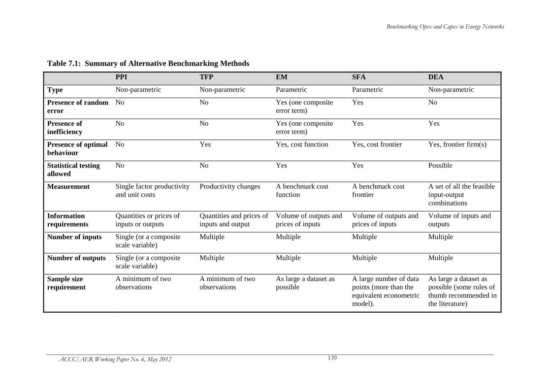
Benchmarking Opex and Capex in Energy Networks
ACCC/AER Working Paper No. 6, May 2012 139
Table 7.1: Summary of Alternative Benchmarking Methods
PPI TFP EM SFA DEA
Type Non-parametric Non-parametric Parametric Parametric Non-parametric
Presence of random
error
No No Yes (one composite
error term)
Yes No
Presence of
inefficiency
No No Yes (one composite
error term)
Yes Yes
Presence of optimal
behaviour
No Yes Yes, cost function Yes, cost frontier Yes, frontier firm(s)
Statistical testing
allowed
No No Yes Yes Possible
Measurement Single factor productivity
and unit costs
Productivity changes A benchmark cost
function
A benchmark cost
frontier
A set of all the feasible
input-output
combinations
Information
requirements
Quantities or prices of
inputs or outputs
Quantities and prices of
inputs and output
Volume of outputs and
prices of inputs
Volume of outputs and
prices of inputs
Volume of inputs and
outputs
Number of inputs Single (or a composite
scale variable)
Multiple Multiple Multiple Multiple
Number of outputs Single (or a composite
scale variable)
Multiple Multiple Multiple Multiple
Sample size
requirement
A minimum of two
observations
A minimum of two
observations
As large a dataset as
possible
A large number of data
points (more than the
equivalent econometric
model).
As large a dataset as
possible (some rules of
thumb recommended in
the literature)
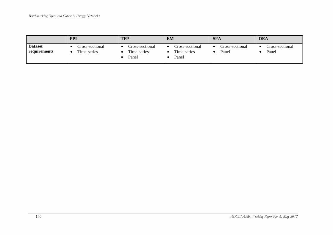
Benchmarking Opex and Capex in Energy Networks
ACCC/AER Working Paper No. 6, May 2012 140
PPI TFP EM SFA DEA
Dataset
requirements Cross-sectional
Time-series
Cross-sectional
Time-series
Panel
Cross-sectional
Time-series
Panel
Cross-sectional
Panel
Cross-sectional
Panel

Benchmarking Opex and Capex in Energy Networks
ACCC/AER Working Paper No. 6, May 2012 141
7.3 Data issues in benchmarking
7.3.1 General data requirements
The cost benchmarking methods require price and/or quantity information on input
and/or output, and sometimes information on various costs and business conditions,
for a sufficiently large number of cross-sectional and/or time-series observations.
They have been used in benchmarking analysis to establish some reference
performance for the sampled businesses – such as own past performance (e.g., trend)
or current industry best-practice or average performance on a regional, country or
international level.
Regardless of the methods used, the availability of a high-quality, reliable and
sufficiently large dataset that covers comparable businesses at a point in time or over
a period of time is essential for the proper application of benchmarking, which
involves an assessment of the efficiency and productivity performance at the business
or industry level.
7.3.2 Potential data problems
Data-point availability can be an issue for each of the benchmarking methods
reviewed. It is a particular issue for the relatively data-demanding parametric
approach (EM and SFA) requiring a large sample size relative to the number of
parameters estimated (i.e., the degree of freedom) – higher degree of freedom for
estimating a regression model means that a larger amount of information is available
so that a better estimate can be derived.
Therefore the choice of the method can be, in part, dependent on the availability of
data. For example, the limited number of regulatory applications of SFA identified,
including Sweden (electricity), Germany (electricity and gas) and Finland
(electricity), takes place in countries where there are a large number of utilities
operating in the sub-sectors. In the UK, the regulator has applied the OLS-type
regression analysis to a relatively small set of 14 utilities. DEA has also been used as
a cross-check against the regression results. As for jurisdiction-based distribution
determinations in Australia, a combination of assessments, particularly the PPI
method, has often been used, possibly due to the very small number of distribution
businesses in a state.
A challenge to relying upon even the simple PPI method and placing a greater weight
on benchmarking distribution businesses in regulatory determinations is the
compatibility of the regulatory data for the utilities compared.
Obtaining high-quality and consistent information across utilities and over time is
equally important for other benchmarking methods to allow like-with-like comparison
and/or to establish representative industry frontier or average performance.
The presence of data errors or noises can also influence the choice of the
benchmarking method. Methods with no account for random errors (e.g., DEA) may
not be suitable for data of low quality. Nevertheless, prior to the application of
benchmarking method, sufficient data checking needs to be done to identify potential
data errors and thus improve data quality.
Benchmarking Opex and Capex in Energy Networks
ACCC/AER Working Paper No. 6, May 2012 142
Data availability and quality is one of the considerations for possible benchmarking
application. The choice of model specifications is often constrained by data
availability and quality. This is particularly the case for academic researchers
working with data in the public domain. In general, the more disaggregated
specifications on potentially heterogeneous inputs and outputs result in more accurate
benchmarking results. For example, specifying skilled labour and unskilled labour
separately may allow better estimation of their respective contribution to the
production than an estimate of their average contribution when an aggregate labour
measure is used. However, it can be very difficult obtaining disaggregated
information data and the quality of such disaggregated information can be a major
issue given the potential cost-allocation problem (i.e., the allocation of
shared/common costs to individual services). Generally, aggregating the inputs
and/or the outputs to an extent that provides a reasonable categorised representation of
the resources used for the provision of the range of output services is required.
As with other industries, the main categories of resources used for electricity
distribution are labour, capital, and material and other input. The major categories of
outputs can be more difficult to specify and requires a good understanding of the
nature of the network services provided by the electricity distributors (as discussed in
subsection 7.4.2 below).
7.4 Model specification issues
7.4.1 Model specifications
To the extent that data are available, there are some common model-specification and
measurement issues for the benchmarking methods other than the PPI method.
As discussed previously, the appropriate input-output specification and functional
form used in benchmarking should be informed by a combination of sound economic
theories, good industry knowledge and rigorous ‘cost driver’ analysis.
In practice, a range of explanatory variables have been used in different
benchmarking studies of electricity distribution businesses. Jamasb and Pollitt (2007)
tabulated the variables that had been used in previous academic studies. Burns,
Jenkins and Riechmann (2005) noted that ‘it is sometimes suggested that the wide
variety of cost drivers that are used in benchmarking analyses imply that there is no
clear set of variables that should be used for benchmarking’. They went on to argue
that different choices of variables in different models primarily reflected the fact that
different studies were seeking to answer different questions. They highlighted three
characteristics that the cost drivers/explanatory variables should satisfy:
Describing the cost drivers that most accurately and comprehensively explain
the costs;
Exogenous environmental factors that affect the costs; and
For which data can be collected consistently across all businesses and with a
reasonable effort.
Regulatory practices for electricity distribution show similarities in the model
specifications, though no two countries reviewed applied benchmarking analysis in

Benchmarking Opex and Capex in Energy Networks
ACCC/AER Working Paper No. 6, May 2012 143
the same manner. Jamasb and Pollitt (2001, p. 125) provided a list of model
specifications that were used by regulators at that time. The most common outputs
modelled are power delivered and customer numbers. The most common input is
opex, either as an aggregate measure, or in a less aggregated form by type of
expenditures such as wages, maintenance, etc. Some measures of physical quantity of
inputs can also be modelled instead of the value-deflated measures. There appears to
be less consistency in environmental variables modelled.
In principle the selection of the key cost drivers should be carried out independently
of considerations of the available data. The practice of choosing the number of
explanatory variables to suit the data has been heavily criticised by Turvey (2006,
p. 104):
Cost comparisons between enterprises can only illuminate differences in their efficiency in
doing what they do if the magnitudes of their tasks can be compared. This is a platitude,
yet failure to articulate it has led some authors to scrabble around among available data to
select a set of ‘explanatory’ variables without displaying any understanding of what the
enterprises actually do and how they do it. Applying different econometric methods to find
which method and which of such variables give the ‘best’ results is very different from
understanding the industry sufficiently well to identify and describe the determinants of
short-run or long-run costs. Unfortunately, data concerning these true determinants are
usually lacking, resort being had by econometrists to using whichever of the limited
available data that they consider most relevant.
One possible approach to choosing the relevant cost drivers is to explore the
implications of an engineering-based model of the regulated businesses. Burns,
Jenkins and Riechmann (2005) described a method previously used in Austria for
selecting cost drivers based primarily on an engineering-based simulation model of a
hypothetical electricity distribution network. Turvey (2006) highlighted the Network
Performance Assessment Model (NPAM) previously used by the energy regulator in
Sweden.
To the extent that data are available, some aggregation and/or approximations are
required to facilitate the high-level benchmarking at the potential cost of generating
errors in measurement. Furthermore, Jamasb and Pollitt (2001, p. 128) concluded that
‘the issue of choosing the most appropriate benchmarking methods and model
specification cannot be settled on theoretical grounds’ and suggested sensitivity
analysis to test the robustness of the results with respect to model specification and
method.
The major issues arising from the review of literature and regulatory practices, as
discussed below, include:
Output specification and measurement;
Input specification and measurement, particularly for the capital input;
Cost measures;
Operating environment factors; and
Functional form.
Benchmarking Opex and Capex in Energy Networks
ACCC/AER Working Paper No. 6, May 2012 144
7.4.2 Output specification and measurement
Demand-side versus supply-side of network services
The output specifications for the multi-dimensions of energy network services
generally cover the demand-side of services (i.e., electricity delivered and/or
customers connected), but may not necessarily cover the supply-side (e.g., coverage
and capacity of the network) and the quality-of-supply (e.g., frequency and duration
of outages) aspects of network operation.
In conducting a benchmarking analysis, a decision as to whether to consider outputs
based solely on demand-side or supply-side models or a mixture of the two has to be
made. In doing so, one has to recognise that the model selected may be biased
towards particular business types.
The demand-side models tend to favour urban distributors with dense networks while
the supply-side models tend to favour rural distributors with sparse network (e.g.,
long line length). Some studies (e.g., those by Dr Denis Lawrence) consider it
important to account for both supply and demand in the TFP analysis and adjust for
different operating conditions. However CEPA (2003, p. 88) considered that the
inclusion of network length as an output variable (or account for network density)
might introduce perverse incentives by encouraging network expansion solely to
improve relative performance.
Turvey (2006, p. 110) pointed out the difficulty of aggregating the concept of service
capacity into a few variables for the purpose of comparing electricity distribution
networks responsible for providing and maintaining the capacity to meet the
maximum demands upon the various parts of the networks with different voltage
levels and at different locations. He questioned the common use of available data on
electricity distributed (MWh) as a proxy for maximum demand and on network length
per customer as customer density variable to explain maximum demand. In his view,
the relevance of these measures depends on networks having similar customer and
load factors. Network efficiencies may be inaccurately estimated because of
business-specific circumstances not adequately described by the available data.
Quality of services measures
Quality of services can be an important issue as these may exhibit substantial quality
differences across utilities or quality changes over time.
A more recent research theme in the academic literature is the incorporation of quality
of services in benchmarking of energy networks, which has been briefly reviewed in
Coelli, Gautier, Perelman and Saplacan-Pop (2010). Of the small number of reviewed
empirical studies quantifying the impact of cost-quality modelling, both the DEA
study by Giannakis, Jamasb and Pollitt (2005) and the SFA study by Growitsch,
Jamasb and Pollitt (2009) found that incorporating quality of services into cost
benchmarking would affect the measured productivity significantly. They argued for
the integration of quality-of-service measures into regulatory cost benchmarking. On
the contrary, Coelli, Crespo, Paszukiewicz, Perelman, Plagnet and Romano (2008)
found that the inclusion of the number-of-interruption measure had no significant
Benchmarking Opex and Capex in Energy Networks
ACCC/AER Working Paper No. 6, May 2012 145
effect upon mean technical efficiency scores estimated from DEA and SFA
respectively.
It is rare in regulatory practices to directly incorporate quality into cost benchmarking.
Instead most of the countries reviewed run separately a quality-of-service
reward/penalty regime. The exceptions may include the Energy Market Authority
(EMA), the Finish regulator, who has taken outage costs (i.e., the cost to consumers
caused by electricity supply outages) into account as part of the total cost for
efficiency benchmarking by DEA and SFA for the determination of business-specific
efficiency target for the regulatory period 2008 to 2011 (see WIK-Consult 2011,
pp. 20-26).
Consistent cross-sectional and time-series data measuring one or more of the three
aspects of quality of services – reliability of supply (SAIDI, SAIFI, CAIDI, MAIFI),
technical quality of services (e.g., number of complaints, distribution network loss or
cost of loss), quality of customer services (e.g., call centre performance) are generally
not available to the economic regulators or the researchers as they have not been
systematically reported by the energy networks.
In addition, there are two reasons for the failure to incorporate quality of services in
the index-number-based TFP analysis: first, the method does not incorporate ‘bad
outputs’ (i.e., a decrease in the measure represents an increase in service-quality
output) easily; and second, it is difficult to value quality improvement to consumers in
order to weigh the quality-of-service output appropriately.
7.4.3 Input specification and measurement
Capital input measures
Of the inputs modelled, capital input is most problematic to measure, which may
explain the common practice of benchmarking opex as opposed to the ‘total cost’
approach. The calculation of the periodic capital input in terms of physical quantity
(and cost) is important for benchmarking analysis, particularly in a capital-intensive
network industry. For production analysis, the proper measure of capital input is the
flow of capital services during a period. A proxy can be the measure of capital stock
in place, which is assumed to be in proportion to the flow of capital services,
regardless of the age of assets. For electricity distribution, physical quantities of two
main distribution assets are commonly modelled – network line length (in
route/circuit kilometres) and installed transformer capacity (in MVa).134
It assumes
constant provision of services at full productive efficiency until the end of the service
life of an asset (‘one-hoss shay’).135
Other depreciation profiles may also be assumed
in the empirical studies; for example, a declining-balance approach to depreciation
called perpetual inventory method (PIM) has generally been adopted in the PEG
studies (see for example, PEG 2004) to construct the constant-dollar replacement cost
of utility assets using detailed capital data over time.
134
The network line length measure models transmission of energy to customer, and the installed
transformer capacity measure captures transformation of high voltage energy to low-voltage energy. 135
A number of researchers in the area consider the one-hoss shay depreciation pattern reasonably
reflect the depreciation process in the electricity distribution. See for example, Makholm and Quinn
(2003, p. 5) and Lawrence and Diewert (2006, p. 217). For a definition of the term, see OECD (2012).
Benchmarking Opex and Capex in Energy Networks
ACCC/AER Working Paper No. 6, May 2012 146
There is an on-going debate in the literature, as well as in the regulatory work, as to
whether capital input is better measured in terms of physical quantity or monetary
value. Some, such as PEG (2004), have argued that the deflated asset value method
provides a better estimate of total capital input as it incorporates other types of major
fixed assets than distribution lines and transformers. Lawrence (2005b) argued
against the use of deflated asset value method for the TFP analysis for Victorian
electricity distribution networks for two main reasons:
The method usually assumes the declining-balance approach to depreciation,
which may overstate the rate of physical depreciation for electricity distribution
networks whose true depreciation profile is more likely to reflect the ‘one-hoss
shay’ or ‘light bulb’ assumption. Therefore, the method is likely to
underestimate the quantity of capital used and overstate the rate of TFP growth
(Lawrence, 2005b, p. 12).
The method is better suited to more mature systems where the asset valuations
are very consistent over time and across utilities, which is not the case for the
Victorian sub-sector.
Analogously, Coelli, Crespo, Paszukiewicz, Perelman, Plagnet and Romano (2008)
measured capital stocks using gross (not depreciated) replacement value. They chose
this in preference to net replacement measure to avoid identifying a business with
significant amount of recent investment as inefficient because of their relative high
net capital stock. They noted two implicit assumptions made in using this measure:
first, the asset age was assumed not to significantly affect service potential; and
second, all operators were assumed to have assets with similar life spans and hence
that annual service potential was proportional to the stock. In their views, these
assumptions were arguably reasonable in their study as all the data came from a single
distribution business who defined and managed very similar policies for investment,
operations and network asset development across the various local distribution units.
In their book on efficiency measurement for network regulators, Coelli, Estache,
Perelman, and Trujillo (2003) includes an entire appendix on capital measurement.
They also recommend the use of undepreciated replacement value measure, if relevant
data are available (Coelli, Estache, Perelman, and Trujillo, 2003, p. 119).
Capital input price can be measured either directly (i.e., annual user cost of capital
that takes account of depreciation, opportunity costs and capital gains) and indirectly
(i.e., realised residual between total revenue and operating and maintenance costs),
which may also drive differences in the measured TFP or other performance
measures. For example, in its critical review of PEG (2004), Lawrence (2005b)
considered that the direct measure reported by PEG appeared to underestimate the
true cost of capital. Nevertheless, the direct measure is more desirable as it
approximates the ex ante cost of capital. However, it is information-intensive and has
many measurement problems with the individual estimation of the depreciation rate,
the opportunity cost and the expected capital gains.
Other input measures
Another major category of inputs is labour. Physical quantity of labour input is
generally measured at the aggregate level; for example, the number of full-time-
Benchmarking Opex and Capex in Energy Networks
ACCC/AER Working Paper No. 6, May 2012 147
equivalent (FTE) staff or total hours worked. The aggregate measure does not make a
distinction between labours of different skills and thus assumes uniform skill
distribution across comparable businesses. Labour quantity can also be measured as
the labour cost deflated by an appropriate labour price index, which may reflect many
inter-business differences, such as skill distribution and wage rate. Depending on
how labour quantity is measured, the labour price can be measured either directly
using a suitable labour price index or indirectly as the total labour cost divided by the
labour quantity measure.
The ‘other input’ variable is generally a ‘catch all others’ category containing
material, fuel and other office expenses. The constant-dollar value measure is
generally used for measuring this variable. For individual expense items within this
category, their respective share to total costs is generally small and therefore does not
warrant separate categorisation and consideration. Specific categorisation may be
needed for some types of expense items (e.g., outsourcing cost) that are sufficiently
large and changes differently from other types of expenses. The increased use of
contract labour also complicates the modelling of labour input as a separate category.
7.4.4 Cost measures
For cost benchmarking, one or more of the four cost measures – operating expenditure
(opex), capital expenditure (capex), total expenditure (totex – the sum of opex and
capex) or total costs incorporating the cost of capital – may be considered. Potential
issues arising from benchmarking opex, capex, totex and total costs are further
discussed in Chapter 8.
It is worth noting that the total-cost approach to benchmarking has been adopted by
the Dutch energy regulator, DTe, in its regulation of electricity transmission and
distribution network (Ajodhia, Petrov and Scarsi 2003). The total cost is the sum of
operating expenditure, depreciation and a standard return on assets. It is used as the
single input factor in the DEA benchmarking. The total cost approach is considered
to be preferable as it creates incentives to improve performance in both the short term
and the long run. However, as noted above, it can be very difficult to measure the
price and quantity of the capital input, and thus their product – capital costs – is
extremely difficult to measure for benchmarking purposes.
7.4.5 Operating environment factors
In addition to the modelling of inputs and outputs in the production, there is also a
need to consider the role of exogenous environmental factors that are out of
management control but may influence business performance. Some benchmarking
methods, such as the parametric approach, allow relevant environmental factors to be
directly included in the modelling. Other methods (e.g., TFP and DEA) generally use
second-stage regression analysis to test the influence of environmental factors on the
estimated raw efficiency and productivity performance.
For electricity distribution businesses, key operating environment conditions may
include (but not be limited to) geographical conditions such as energy density,
customer density, network density, customer mix and underground relative to
overhead network. The literature on TFP studies suggests that energy density and
customer density are generally found to be the two significant operating environment

Benchmarking Opex and Capex in Energy Networks
ACCC/AER Working Paper No. 6, May 2012 148
variables in energy distribution studies. See for example, AEMC (2008) and
Lawrence, Diewert and Kain (2007). In their study of the productivity of the Swiss
gas distribution sub-sector using SFA, Farsi, Filippini and Kuenzle (2007) pointed out
the importance of environmental and output characteristics such as customer density
and service area size.
7.4.6 Functional forms
For non-parametric methods (TFP and DEA), no specification of a functional form for
the production or cost function is required. For a parametric approach (EM or SFA),
an appropriate functional form for the production or cost function is used to capture
the underlying production technology. A variety of functional forms have been used
in empirical studies. The most commonly adopted forms are the simple
Cobb-Douglas function and the more complex transcendental logarithmic function
(translog for short).
The Cobb-Douglas functional form is a restrictive representation of the underlying
production technologies. That is, the limitation of the Cobb-Douglas is that it
automatically imposes restrictions on resulting substitution possibilities between
inputs a priori, regardless of whether it is desirable. This will generate results that are
biased if the underlying industry technology is not Cobb-Douglas in nature. This
problem is referred to in the literature as a ‘lack of flexibility’ in the functional form.
The translog function is a direct generalisation of the Cobb-Douglas function,
allowing for all squared and cross-effects terms for output quantity and input prices
variables to be included in the cost function (or all squared and cross-effects terms for
input quantity variables in the production function). This functional form is more
flexible such that it provides a second-order approximation to any well-behaved
underlying cost function at the mean of the data (Kumbhakar and Lovell, 2000,
p. 143). That is, the substitution possibilities between inputs, such as capital and
labour, can be better identified without restrictions or limitations. This means that the
translog functional form is more likely to generate results that are consistent with neo-
classical microeconomic theory, with fewer providing biased results.
The translog function is capable of producing an estimated model of an industry that
includes the following important underlying economic properties:
Domain: the cost function is a positive real-valued function defined for all
positive input prices and all positive producible output.
Monotonicity: the cost function is non-decreasing in output and non-decreasing
in input prices.
Continuity: the cost function is continuous from below in output and continuous
in input prices.
Concavity: the cost function is a concave function in input prices.
Homogeneity: the cost function is linear homogenous in input prices.
Following the estimation of the model, these properties can be tested. Estimated
translog models may not contain these economic properties. This may suggest

Benchmarking Opex and Capex in Energy Networks
ACCC/AER Working Paper No. 6, May 2012 149
problems with data. In this case, the translog results would not be persuasive. In
addition, translog functions may fail to produce statistically significant results for
some samples due to the potential multicollinerity problem.136
The translog functional form has become popular in recent applied production studies.
However, flexible functional forms tend to have an increase in the number of
parameters to estimate econometrically,137
requiring a higher number of data points
for estimation. Therefore there is a trade-off between the extent to which an
econometric functional form imposes few restrictions on the underlying production
process and the number of data points that is needed to estimate that function.
Some empirical studies have used statistical testing (e.g., the generalised likelihood-
ratio test) to determine whether the Cobb-Douglas or the translog functions are best
suited (Coelli, Rao, and Battese, 1998, p. 201).
Using Monte Carlo simulations, Guilkey, Lovell and Sickles (1983) compared three
flexible functional forms, namely translog, generalised Leontief, and generalised
Cobb-Douglas – and found that the translog form performed at least as well as the
other two and provided ‘a dependable approximation to reality, provided that reality is
not too complex’.
Nevertheless, specifying a particular functional form limits the range of technologies
that can be characterised. Depending on the existing knowledge about the underlying
production technology in energy networks, an appropriate functional form or
alternative functional forms may be chosen for the cost benchmarking.
7.5 Insights into benchmarking of energy networks
7.5.1 Addressing potential data issues
As noted in section 7.3, data availability and quality are considerations for the
possible benchmarking application. Effort should be made by researchers or
regulators to access larger datasets and improve the quality of benchmarking data.
According to Lowry, Getachew and Hovde (2005, p. 91), this can be achieved by the
accumulation of panel data and the greater use of international benchmarking.
Panel-data analysis
Quality panel data covering several energy utilities over a period of time, if available,
will not only increase the sample size, but also address some shortcomings with the
use of cross-sectional data. However, the lack of quality panel data to facilitate such
an analysis often limits the use of benchmarking methods.
136
Multicollinearity is only a problem if accurate estimates of individual parameters (e.g., price
elasticities in a demand function) are needed. For benchmarking analyses using econometric methods,
the research interest is the efficiency estimates, which are linear combinations of a large number of
estimated coefficients. Multicollinearity in a benchmarking model may not affect the model’s
efficiency prediction performance. 137
For example, for a Cobb-Douglas production with n+1 parameters, the corresponding translog
production function has a total of (n+1)(n+2)/2 parameters.
Benchmarking Opex and Capex in Energy Networks
ACCC/AER Working Paper No. 6, May 2012 150
With one-year data where some observations may be strongly influenced by
unexpected events (e.g., severe weather condition) or one-off major capital
expenditure made, the benchmarking results may not reflect the longer term
performance of these utilities or the overall performance of the sub-sector examined.
Furthermore, panel data can also be used to measure business- and industry-level
performance changes over time, such as TFP changes and its sources such as technical
changes (i.e., frontier shift) and efficiency change (i.e., catch-up).
In the academic literature there have been mixed views regarding the usefulness of
panel data for benchmarking analysis. Burns and Weyman-Jones (1996) found panel
data to be useful in addressing the shortcomings of cross-sectional data. In particular,
some variables that are particularly important for cross-sectional comparison may not
be required for panel-data analysis. In their study in relation to applying SFA to
electricity distribution in England and Wales, panel data suggested two main
determinants of opex – customer numbers in an area and simultaneous maximum
demand. A series of papers involving Farsi and Filippini (e.g., Farsi and Filippini
(2004), Farsi, Filippini and Greene (2006)) examined whether some limitations of
frontier models can be overcome with panel data for the Swiss electricity distribution
businesses. Their results tend to confirm that robustness problems reported in relation
to cross-sectional data might also apply to panel data.
The use of panel data may create its own problems. Value measures (e.g., for some
inputs) need to be deflated to derive the equivalent constant-dollar measures.
However, the availability of appropriate price deflators can be an issue. Moreover,
data may be inconsistent or discontinued over time due to changes in definitions,
accounting standards, or data providers. These may limit data comparability over
time and across businesses. It is noted that the lack of quality panel data has
prevented the Ofgem from using panel data for benchmarking analysis in its earlier
price control reviews. It is not until the most recent price control review (2009-10 to
2014-15) that panel-data regression was applied to its benchmarking analysis. The
Ofgem considered that one of the limitations of its panel-data analysis was the
assumption of constant effect of cost drivers over time, which might not necessarily
be the case (Ofgem, 2009, p. 74).
International benchmarking
Another way to increase the sample size is to include energy utilities operating in
other countries in the dataset. By doing international benchmarking, the industry
frontier or performance can be strongly influenced by international best-practice
utilities rather than the domestic best-performers.
In the academic literature, some studies, including Jamasb and Pollitt (2003), Estache,
Rossi and Ruzzier (2004) and Goncharuk (2008), have focussed on comparing
utilities in one country to utilities in other comparable countries. The key issues
expressed in relation to the application of international benchmarking relate to the
availability of data, exchange rate issues and technical issues for addressing country
differences in labour price, cost of capital, regulatory and environmental factors and
so on. Some trade-off has to be made between increasing sample size and
maintaining homogeneity (or adjusting for heterogeneity) of the sample utilities.

Benchmarking Opex and Capex in Energy Networks
ACCC/AER Working Paper No. 6, May 2012 151
In recognition of the increasing complexity in conducting international benchmarking,
Estache, Rossi and Ruzzier (2004) considered that there would be net benefits of good
coordination across regulators in establishing an international database for
benchmarking. Jamasb and Pollitt (2003, pp. 30-31) made some recommendations on
the approaches to co-ordinating international benchmarking exercises, including:
Agreement on long-term commitment and procedures for data collection,
common templates, and submission deadlines for data standardisation;
Identifying and defining a minimum set of input, output, and environmental
variables for data collection;
Other desirable variables including maximum demand, transformer capacity,
service area, quality of service, and voltage-based physical and monetary
breakdown of assets;
Collecting data of a representative sample covering different size groups and
types of utilities, starting from the most recent years and accumulating over
future years;
Discussion on benchmarking models, functional forms and weightings; and
In-depth examination of the extent of similarities and differences between the
inefficient firms and their peers to support the benchmarking results.
The development of an internationally consistent dataset that is useful to
benchmarking would be beneficial to regulators across countries. For regulatory
applications, international benchmarking has more often been used for benchmarking
transmission service providers given their very limited number in a single country.
For example, the Agrell and Bogetoft (2009) study on electricity and Jamasb,
Newbery, Pollitt and Triebs (2008) study on gas, both commissioned by the Council
of European Energy Regulators (CEER), provided a useful input into the German
approaches to efficiency benchmarking and regulation of the transmission sub-sectors.
Caution
Caution should be exercised when colleting the panel data and/or international data to
ensure that the dataset contains the most comprehensive information that is broadly
consistent over time and comparable across energy utilities. In-depth examination of
the data is required to ensure consistency, comparability and quality. For
benchmarking analysis, data may need to be adjusted to ensure a valid comparison for
energy utilities providing slightly different services and/or operating in different
environments.
7.5.2 Addressing model specification problems
A good understanding of the nature of the production process implemented by the
energy utilities in transforming labour, capital and other resources into utilities’
services provided is fundamental to the development of sound benchmarking analysis.
The economic theory and industry knowledge, together with comprehensive cost-
driver analysis and engineering studies, can be useful for informing the development
of model specifications and production functional forms.

Benchmarking Opex and Capex in Energy Networks
ACCC/AER Working Paper No. 6, May 2012 152
For alternative model specifications, it is important to consider the assumptions
underpinning the model and their implications for the measurements. If there is no
strong theoretical foundation favouring a particular model specification, sensitivity
analysis can be conducted to examine the robustness of the results.
A common theme among much of the reviewed literature has been the advocacy of
the use of sensitivity analysis as part of any benchmarking technique. A number of
authors have suggested that this approach is necessary to ensure that the
benchmarking results (e.g., efficiency scores and rankings) are robust and accurate.
These sources include the IPART (1999), Farsi and Filippini (2004), and Jamasb,
Nillesen and Pollitt (2004). It also appears from the literature that the application of
the DEA method can be particularly sensitive to model specification. DEA does not
incorporate any error terms and thus can be very sensitive to measurement errors and
selection of variables.
7.5.3 Choice of methods
Some interesting and relevant discussion on the choice of benchmarking method is
presented by Coelli, Estache, Perelman and Trujillo (2003). Relevant factors
affecting the potential use of benchmarking and the choice of the benchmarking
method include:
Industry characteristics: How many like businesses in the sample that can be
used to benchmark? As previously noted, some methods require a sufficiently
large number of observations and thus may not be particularly suitable for an
industry with relatively few comparable utilities domestically.
Data availability and quality: the use of panel data or international benchmarking
to address the data-availability issue has a challenge in obtaining quality and
consistency data for comparable utilities. The extent of data noises present will
also affect the methods that can be chosen.
The intended use of the benchmarking results under the regulatory regime: for
example,
the benchmark industry-average productivity growth rate can be derived
from the index-number-based TFP method; or
the comparative performance of a benchmark frontier, average or other
businesses, whichever is considered appropriate, can be derived from one
of the non-index-number-based methods (EM, DEA and SFA).
Each of the five benchmarking methods provides useful information for
benchmarking the utilities regulated. However, depending on the legal and regulatory
requirements, one or both of the two types of methods may be used. For regulatory
applications, TFP is generally used for estimating the frontier-shift component while
comparative performance from DEA or regression analysis has been used to assess
the catch-up component of the X factor. Under the Building-block-model (BBM)
adopted in Australia, there is no need to estimate the productivity-offsetting X factor
directly. Under the BBM, the X factor in the CPI–X form of price or revenue path is
simply a smoothing factor. The TFP results may be used as a cross-check for the
future productivity change implied in the forecasts proposed by the utilities.

Benchmarking Opex and Capex in Energy Networks
ACCC/AER Working Paper No. 6, May 2012 153
Taking into account these factors, judgements need to be made for the choice of
appropriate benchmarking methods. It is also important to note that different
benchmarking methods may differ in many aspects and some of the differences may
affect the results differently. For example, using the same set of cost data, DEA and
SFA methods estimate the cost frontier formed by the best-practice businesses, which
can be substantially different from the estimated cost function formed by the average
of the sample under the conventional EA method.
Therefore, while one method may be favoured, sensitivity analysis that examines the
robustness of results with respect to more than one technique is desirable. Bauer,
Berger, Ferrier and Humphrey (1998) and Rossi and Ruzzier (2000) proposed a set of
‘consistency conditions’ that should be met by efficiency estimates generated from
different methods to ensure that they are mutually consistent. Specifically, the
consistency conditions are:
the efficiency scores generated by the different methods should have
comparable means, standard deviations, and other distributional properties;
the different methods should generate approximately the same ranking of the
efficiency scores;
the different methods should identify mostly the same group of observations as
‘best practice’ and as ‘worst practice’;
all of the useful methods should demonstrate reasonable stability over time, i.e.,
tend to consistently identify the same institutions as relatively efficient or
inefficient in different years, rather than varying markedly from one year to the
next;
the efficiency scores generated by the different methods should be reasonably
consistent with competitive conditions in the market; and
the measured efficiencies from all of the useful methods should be reasonably
consistent with standard non-frontier performance measures, such as return on
assets or the cost/revenue ratio.
The set of consistency conditions requires both internal consistency (i.e., consistent
efficiency levels, rankings, and identification of best and worst performers) and
external consistency (i.e., consistent over time and with competitive conditions in the
market, and with standard non-frontier measures of performance) across alternative
methods and model specifications. Estache, Rossi and Ruzzier (2004) explored the
implications for price cap regulation if consistency in efficiency levels and rankings is
not met. They considered consistency in identifying best and worst performers most
important as it would facilitate public naming and shaming those that were not
performing well.
Consistency analysis can be performed to improve robustness of benchmarking results
with respect to alternative methods and model specifications. Wherever the results
from alternative methods and model specifications differ materially, justifications for
the use of the results need to be provided.
Benchmarking Opex and Capex in Energy Networks
ACCC/AER Working Paper No. 6, May 2012 154
7.6 Conclusions
The review into benchmarking of energy networks shows that benchmarking can be
used to measure industry average performance and/or comparative performance of
individual energy network service providers. Overall, benchmarking has been used
widely in the literature and in the regulatory work. It provides information about the
performance of comparable energy networks and is of potential use to the regulators.
The outcome of benchmarking may depend on the availability, comparability and
quality of data, choice of method, and selection of model specification. As discussed
previously, the appropriate input-output specification and functional form used in
benchmarking should be informed by a combination of sound economic theories,
good industry knowledge and rigorous ‘cost driver’ analysis. To the extent that data
are available, some aggregation and/or approximations are required to facilitate the
high-level benchmarking at the potential cost of generating errors in measurement.
Where the issue of choosing the most appropriate benchmarking methods and model
specifications cannot be settled on theoretical grounds, sensitivity analysis is needed
to test the robustness of the benchmarking results.
Robust benchmarking analysis is highly desirable and as such, benchmarking results
should be examined against the set of the Bauer consistency conditions proposed in
the literature. In some cases inabilities to produce similar results with alternative
model specifications and methods require further investigation so that benchmarking
outcomes can be supported by more rigorous analysis; otherwise caveats for the
conclusions should be provided.
Other insights into benchmarking energy networks are also provided, suggesting the
potential use of panel-data analysis and international benchmarking. However,
caution should be exercised when collecting and analysing the data to ensure that the
information contained in the larger dataset is consistent over time and comparable
across businesses.
Benchmarking Opex and Capex in Energy Networks
ACCC/AER Working Paper No. 6, May 2012 155
Chapter 8 Implementation issues in achieving effective benchmarking
8.1 Introduction
The preceding chapter reviews the various issues when applying benchmarking
methods to energy networks. In particular, it has considered potential data availability
and quality issues and model specification problems. This chapter follows by
considering the broader challenges that the regulators may face when applying
benchmarking of operating expenditure (opex) and capital expenditure (capex) in the
electricity and/or gas sub-sectors (distribution and/or transmission).
The chapter is divided into six sections. Section 8.2 provides a definition of opex and
capex and explores the potential challenges arising from the measurement and
comparability of the two categories of expenditure across regulated utilities. Section
8.3 is a consideration of service quality and reliability in regulatory benchmarking –
how is quality-of-service performance defined, can it be quantified, are there tradeoffs
between quality and efficiency, and can service quality be benchmarked? Section 8.4
examines the role of benchmarking as an informative tool and as a deterministic tool.
For benchmarking tools, informativeness and determinism are not substitutes; rather it
is argued that they may be sequential complements in the adoption of a regulatory
benchmarking program. Section 8.5 maps the implementation process when a
regulatory benchmarking program is introduced. Finally, section 8.6 explores the
opportunities and possibilities that may enhance the use of benchmarking in the
regulatory context, considered in the light of the available techniques and data
reviewed in previous chapters of this paper.
8.2 Operating expenditure, capital expenditure and total expenditure and their
tradeoffs
Benchmarking a regulated utility’s performance normally involves a standardisation
and comparison of opex, capex and/or total expenditure (totex), where the latter is the
sum of the former two expenditures.
Operating expenditures and capital expenditures are accounting categories that
itemise the incurrence of capital and operating costs. If a regulator adopts
benchmarking, it is important that the categorisation and incurrence of such cost is
transparent, accurate and comparable across utilities.
However, accounting classifications in many respects are subjective – for example,
accounting standards between Australia and the United States differ on what items
should be immediately expensed and what items should be capitalised. Under the
International Financial Reporting Standards – that represent the standards followed by
the European Union, Australia and many emerging economies – Research and
Development (R&D) expense is capitalised and amortised. However, in the United
States, the Generally Accepted Accounting Principles require an immediate expensing
of R&D (see Cohen, 2005, pp. 58-59).
In a regulatory setting, how opex and capex are categorised may directly affect the
regulated utility’s path of allowed revenues. Therefore, transparency, accuracy and
comparability of cost categorisation and cost incurrence are crucial for effective
regulation of utilities, whether benchmarking is undertaken or not.

Benchmarking Opex and Capex in Energy Networks
ACCC/AER Working Paper No. 6, May 2012 156
Operating expenditure
Opex pertains to operating and maintenance expenditure items that are expensed for
the utility’s income year. It includes both variable and fixed costs with respect to
variations in the production level. Some types of opex are costs which are normally
direct costs expensed for a utility’s income year that also vary with output. For
example, intermediate inputs/materials, fuel or electricity, and some types of labour
and labour-related expenses (e.g., overtime payments for labour).
A large proportion of opex, including some labour-related expenditure, is fixed over
certain ranges of output(s). They are quasi-fixed inputs; for example, direct cost
related to the activities undertaken, such as maintenance expenditure and
transportation cost; and indirect costs or operating overheads, such as, leases,
insurance, administration, marketing, human resources and IT support. As these costs
are generally shared among services and are not responsive to units of outputs,
additional cost drivers are applied to allocate the costs to individual services or
activities.
While depreciation of capital stock is normally considered to be an operating cost
(and there are direct and indirect cost components to depreciation), this annually
expensed item is normally outside the measured opex and is treated separately as the
‘return-of-capital’ component in a building-block model.
Capital expenditure
Capex pertains to an outlay that will generate a flow of future income over time (i.e.,
beyond the income year). Capex is commonly recorded on the cash-flow statement as
‘payment for property, plant and equipment’ or similar items. The resulting addition
to fixed assets will be reflected on the balance sheet and then depreciated or amortised
over time. Relevant expenditure items include: the purchase of fixed assets;
upgrading a fixed asset or repairing a fixed asset that will extend its useful life; and
developing intangible assets through R&D, or acquiring intangible assets such as
copyrights, trademarks, trade secrets and patents.
If opex is capitalised, such as wage and installation costs, then the assessment of
capex becomes problematic because that capitalisation of opex may be idiosyncratic
across utilities. Regulated utilities may have an incentive to capitalise opex in order
to inflate the regulatory asset base if allowance for capital cost is subject to rate-of-
return regulation, rather than external benchmarking. In a review of incentive
regulation of electricity distribution and transmission networks, Joskow (2006, p. 2)
pointed out that:
In the UK, for example, the initial failure of regulators to fully understand the need for a
uniform system of capital and operating cost accounts as part of the foundation for
implementing incentive regulation mechanisms has placed limitations on their effectiveness
and led to gaming by regulated firms (e.g. capitalizing operating costs to take advantage of
asymmetries in the treatment of operating and capital costs).
Since benchmarking requires standardised definitions and classifications of opex and
capex, an effective benchmarking program will detect such gaming – unlike the
building-block model, which permits idiosyncratic incurrence of costs.

Benchmarking Opex and Capex in Energy Networks
ACCC/AER Working Paper No. 6, May 2012 157
Benchmarking operating expenditure
Benchmarking opex is subject to particularly challenging data-quality and data-
comparability problems. This is particularly the case when benchmarking is
performed at an activity and/or business segment level. However, when opex as an
aggregate is compared across utilities, the idiosyncratic processes employed by
individual utilities in asset and cost allocation are diluted, and measures of aggregate
per unit (i.e., a standard unit of single output or a standard combination of multi-
product output) become more important.
As noted above, effective opex benchmarking requires clear and sound rules for cost
classifications and allocation that are uniformly and consistently applied across
utilities. These cover, for example, allocations of shared costs across services and
classifications of capex as opposed to operating and maintenance expenditure.
Benchmarking capital expenditure
Regulators have often adopted a bottom-up approach to reviewing the reasonableness
of certain categories of expenditure (e.g., asset replacement expenditure) or total
capex proposed by an individual utility. Simple capex benchmarking, such as trend or
ratio analysis, has also been employed to assess the efficiency of capex.
Benchmarking capex against other utilities has not been consistently relied upon,
possibly due to significant differences across businesses in terms of asset ages,
investment pattern, network capacity utilisation and other requirements.
Regulatory treatment of capex could potentially be different from opex. The
building-block model approach includes an allowance for cost of capital, which is the
product of the weighted average cost of capital (WACC) and the value of the
regulatory asset base that reflects changes to assets due to depreciation and addition.
Benchmarking total expenditure
Benchmarking totex involves a comparison of total expenditure (i.e., the sum of opex
and capex) across utilities once controlling for the following, among other factors that
may affect the comparability of cost incurrence:
scale, scope, sequence and density economies; 138
geography and topography of the network of operations (partly relating to
density);
composition of consumers; and
timeframe.
138
Since Adam Smith’s observation of the division of labour in a pin factory, economists have
recognised that production involves a sequence of steps. And these steps are often integrated within a
single entity – such as, processing raw materials, assembling inputs, and the sequences of design,
production and marketing. And the sequence of steps within a single entity defines its boundary.
Economies of sequence arise when it is less costly to integrate a sequence of production steps within
one producer rather than having that sequence of steps undertaken separately and independently by
multiple producers. Producers will continue to vertically integrate until the economies of sequence of
integrating production processes/steps are exhausted. See Spulber (1989).
Benchmarking Opex and Capex in Energy Networks
ACCC/AER Working Paper No. 6, May 2012 158
Totex benchmarking requires identification and comparability of opex and capex
without the potential requirement that utilities possess the same input
shares/production technology; and the same degree of uniformity, standardisation and
comparability of opex and capex. In other words, this is perhaps a less intrusive
approach to benchmarking economic performance across utilities.
Benchmarking totex has further advantages compared to benchmarking opex or capex
alone.
Firstly, using totex avoids the potential gaming problem when the two categories of
expenditure (i.e., opex and capex) are subject to asymmetric regulatory treatment.
Benchmarking of one but not the other category of expenditure may provide an
incentive to change the composition of inputs in both the short run and long run. The
short-run change may involve an accounting re-classification of opex and capex items
so that the expenditure item that is subject to the more stringent assessment of
benchmarking may be under-reported. Further, the regulated utility may have an
incentive to change its input technology – inducing a long-run substitution away from
the benchmarked expenditure toward the expenditure category that is not subject to
benchmarking. This will not promote cost efficiency.
Secondly, totex benchmarking avoids another ‘gaming’ problem that may arise from
benchmarking opex alone. Under opex benchmarking, the regulated utility may have
an incentive to split into a number of micro-entities that engage in related-party trade
of inputs, as opposed to an internal allocation of inputs within the single utility. The
complex operational structure and large number of related parties and interposed
entities associated with some energy utilities is consistent with the disincentive to
realise economies of scale, scope, sequence and density within a single entity, and
gives rise to regulatory concern of the efficiency of the structure. Totex
benchmarking may capture a wider view of the overall efficiency of the regulated
entity compared to its peers and assist in identifying whether such operational
structures are, in fact, inefficient.
Moreover, under the related-party trade arrangement, the purchase of inputs is more
likely to be capitalised. For example, suppose an electricity distribution pole had to
be replaced, in which case the associated opex and capex may be clearly itemised.
However, if the utility purchased the service from a related party, the entire outlay
may be more likely to be capitalised, so that the opex component will be under-
reported or not reported at all. This is because the installation service is purchased
from another ‘entity’ that is contracted to supply the fixed assets and is therefore
classified as a capex item. Financial Statement practitioners warn about excessive
capitalisation. Examples include the capitalisation of wages and associated costs,
installation costs and development costs (See, Hey-Cunningham, 2006, p. 321).
The resulting under-reporting of opex will provide the regulator with an impression
that the efficient level of opex is being incurred, when, in fact, the focus on opex only
has elicited a ‘waterbed effect’ of reclassifying and moving costs toward expenditure
Benchmarking Opex and Capex in Energy Networks
ACCC/AER Working Paper No. 6, May 2012 159
items that are not benchmarked.139
In this case, the regulated utility has morphed into
micro-entities so that opex can be redefined as capex.
Notwithstanding, totex benchmarking can be challenging, given the inherent data
quality and comparability issues. There is also a specific aggregation problem
associated with totex being an aggregate measure; that is, there are potentially more
sources of annual fluctuations in totex as opposed to opex or capex respectively.
More importantly, totex is subject to the lumpy, indivisible and cyclical nature of
investment, which may result in yearly fluctuations of expenditures, and the
expenditure patterns differ substantially across utilities. It can be problematic to
compare totex across utilities using yearly data that sum up infrequent capex
incurrence and yearly opex expenditure incurrence.
Therefore benchmarking totex in short timeframes is not feasible for energy utilities
that invest in transmission or distribution assets of very long service life. It may
require a longer timeframe (than a typical five-year regulatory period) to establish
representative capex profiles at the utility level unless there are also independent
assessments of capex, and to a lesser extent, of opex, to control for any fluctuations in
these expenditures from year to year.
Benchmarking total cost
Another integration approach is to benchmark yearly opex and flow of capital services
– that is, total cost measured as the sum of opex, the return on capital and the return of
capital each year – so that there is increased consistency of expenditures over time.
If net present value is zero for all projects undertaken, then comparing capital
expenditure across utilities is equivalent to comparing the cash flows (return on and
return of capital) across utilities over time.
However, such benchmarking may present its own data availability and comparability
challenges. The approach can be more information-intensive as it requires not only
historical series of capital investment, but also an asset valuation to start with.
Furthermore, the capital prices and depreciation profiles (asset valuation, asset life
and depreciation pattern) can be substantially different across utilities. There are
differences in utilities’ accounting policy on net residual or scrap value of the assets.
Issues may, therefore, arise with the measurement of the volume of capital services
consumed periodically. When a business makes a sunk, long-lived investment, the
allocation of the cost of that investment to any year of the life of the asset will affect
estimates of efficiency of the business. This is because efficiency estimates are
usually made over a relatively short period, such as one year. It is therefore necessary
to benchmark expenditure of several or more years, and that depreciation profiles are
assumed to be the same across utilities.
Moreover, if the asset is depreciated based on estimated levels of productivity,
incorporating these estimates into the relative efficiency performance of businesses
may involve circular reasoning. Turvey (2006) suggests that circular reasoning can
139
The ‘waterbed effect’ in this context occurs when the regulatory scrutiny and subsequent cost
reductions in one expenditure category shift the effort of the producer toward an equi-proportionate
uplift in expenses in other expenditure categories so that allowed revenue remains unchanged.

Benchmarking Opex and Capex in Energy Networks
ACCC/AER Working Paper No. 6, May 2012 160
be avoided by measuring the volume of capital services that is independent of what it
actually produces. This can be achieved by measuring capital services ex ante, from
the time of asset commissioning, while measuring output ex post, at the time of
production, both at constant prices.
8.3 The consideration of service quality and reliability
As outlined in chapter 7, quality of service can be an important issue for the regulator
when undertaking benchmarking. The requirement that utilities achieve cost savings
on the basis of benchmarking studies should not be at the expense of service quality.
The regulatory benchmarking of service standards across network operators is a
challenging task which requires, first, a standardised and quantifiable definition of
reliability and service quality.
Reliability can be thought of and measured differently in various industries and within
industries. For example, in telecommunications one may measure reliability by the
number of call drop outs, network downtime, or number of line faults. The measures
will vary depending on whether a mobile or fixed line network is considered. On the
other hand, for an airline industry, measuring reliability may involve consideration of
flight cancellations, on-time performance, or accident rate.
Often it will be possible to agree on a common set of indicators. For example, in
energy, there are a number of distribution reliability indicators produced by the
Institute for Electrical and Electronics Engineers (IEEE), which is an international
body that sets service standards for network industries. The IEEE Standard 1366-
2003 focuses on the following measures of network reliability which quantify service
interruptions across electricity network providers:140
SAIFI – System Average Interruption Frequency Index;
SAIDI – System Average Interruption Duration Index; and
CAIDI – Customer Average Interruption Duration Index.
In addition to the above, a number of other reliability measures are sometimes
considered. In particular, the Australian Energy Regulator (AER)’s Service Target
Performance Incentive Scheme focuses on three parameters; namely unplanned
SAIFI, unplanned SAIDI and a third parameter which measures very short term
interruptions, MAIFI – Momentary Average Interruption Frequency Index.141
Service quality in other dimensions can also be considered using a number of
different measures. Usually these measures relate to customer satisfaction, and can
vary between industries and customer groups. For example, large energy customers
may only be concerned with network reliability to ensure service quality, whereas
140
See the Institute for Electrical and Electronics Engineers website, http://www.ieee.org/index.html
and IEEE (2006). 141
MAIFI is only used for some jurisdictions. AER (2009c, p. 9) prescribed that ‘Where the DNSP
demonstrates to the AER it is unable to measure MAIFI, a DNSP may propose a variation to exclude
MAIFI in accordance with clause 2.2, for a regulatory control period or a portion of a regulatory
control period’.
Benchmarking Opex and Capex in Energy Networks
ACCC/AER Working Paper No. 6, May 2012 161
residential telecommunications customers may require prompt installation of lines and
rectification of line problems, help-desk availability, simple billing process, etc.
Although common measures can be established, it is important to note that
benchmarking should take into account any specific differences across utilities. For
example, in measuring reliability of energy networks, it is important to consider
reliability measures under normal operating conditions, and account for major events
separately. As noted above, most of energy reliability measures are related to service
interruption. However, these measures can be dominated by a single major event,
such as a storm or a flood. While the response to the major event can be accounted
for as a measure of reliability, any benchmarking method would need to isolate these
events from benchmarking under normal operating conditions.
Further, when benchmarking, it may be necessary to recognise factors that affect
reliability levels, which may not be controllable by the benchmarked utilities. In case
of energy networks, these may include:
Definition and data classification – e.g., What is a major event? What is
classified as an interruption?
Data-collection process – how and when are outages reported?
Service territory – geography, weather and vegetation patterns; and
System design – urban, rural, and remote overhead/underground wiring.
Of course, different service quality and reliability levels may be associated with
varying levels of expenditure. Cost benchmarking would therefore need to consider
service quality and reliability levels in the context of cost incurred in attaining these
levels. Both service quality and reliability, and cost would need to be controlled for
factors outside management control. For example, service quality and reliability
performance could be compared to the average cost per user separately for central
business district, urban and rural areas.
Further challenges arise with the aggregation of service capacity, which can
determine service quality. It is possible to express the service capacity of an
individual piece of equipment. But questions arise as to how to express the capacity
of an entire network which has the potential to deliver different volumes of electricity
at different voltage levels at different geographic locations. According to Turvey
(2006), benchmarking studies have sought to compare the performance of electricity
networks using measures of throughput (MWh) and line length as a proxy for
measures of capacity at different locations. Turvey (2006) suggested that these
measures were appropriate only when certain conditions were satisfied.
While few studies explicitly have considered service quality as an output variable (see
Coelli, Crespo, Paszukiewicz, Perelman, Plagnet, and Romano, 2008), service quality
is a crucial consideration in benchmarking – the downside risk of ignoring service
quality is that utilities that seek or are required to achieve cost efficiencies may do so
at the expense of service quality.
The main difficulty, however, is likely to lie in the comparison between benchmarked
utilities. While some may choose greater levels of reliability and service quality at

Benchmarking Opex and Capex in Energy Networks
ACCC/AER Working Paper No. 6, May 2012 162
higher cost, others may opt for lower levels. Ideally, levels would be set such that the
marginal benefit to the average consumer from greater service quality or network
reliability equals the marginal disbenefit from the higher service cost. These are
difficult to measure empirically, and internationally individual utilities are usually
allowed to set their own targets. Further, as customer groups may be characterised by
different attitudes toward service quality and reliability – indeed it is likely that
different customer groups of each individual utility may exhibit varying attitudes – it
is difficult to determine whether any utility is making a sub-optimal cost-service level
choice.
In Australia, the AER has already set reliability targets (SAIDI, SAIFI and, in some
jurisdictions, MAIFI) for electricity distribution utilities, but the other service quality
standards are set by the jurisdictions. The service quality targets are part of the
AER’s national service target performance incentive scheme focusing on supply
reliability and customer service (AER, 2011, p. 69):
The national scheme generally provides financial bonuses and penalties of up to 5 per cent
of revenue to network businesses that meet (or fail to meet) performance targets. The results
are standardised for each network to derive an s factor that reflects deviations from target
performance levels. While the scheme aims to be nationally consistent, it has flexibility to
deal with the differing circumstances and operating environments of each network.
With an established institutional and legal structure of standards of service quality
already specified and in place, the above challenges in controlling for service quality
standards when undertaking cost benchmarking may be less numerous and/or less
onerous.
8.4 Benchmarking: an informative tool and a deterministic tool
Benchmarking performance can be used to inform the regulatory approach and also
determine regulatory decisions. The informative and deterministic dichotomy is
drawn from papers that identify issues with the efficacy of benchmarking, such as
Shuttleworth (2005) and Lowry and Getachew (2009b), and thus the dichotomy
connotes substitutability between the two tools. However, benchmarking as an
informative tool is not a substitute for benchmarking as a deterministic tool – rather,
the two tools are sequential complements in the development of a program of
regulatory benchmarking. The complementarities that exist between informativeness
and determinism are highlighted through an exposition of these two stages in a
regulatory benchmarking program.
Informativeness
Informativeness characterises the first stage of regulatory benchmarking which
consists of defining an inter-utility set of expenditure parameters in consultation with
stakeholders, collecting the data, and refining the data to achieve the required quality
and comparability.
The aim of benchmarking is to improve the efficiency and competitiveness of
regulated utilities. Utilities may only be deemed to be profitable, efficient and
competitive when compared to competitors in the same industry or comparable
businesses. For example, whether or not a utility is profitable can only be ascertained
if it is known what constitutes an opportunity cost or normal rate of return for the
Benchmarking Opex and Capex in Energy Networks
ACCC/AER Working Paper No. 6, May 2012 163
market/industry. The relativities determine the regulatory information requirements –
the regulator is not required intrusively to collate granular data from utilities with the
object of constructing a surreal and ‘optimal’ benchmark. Benchmarking against a
theoretical optimum would be analogous to the futility of central planning where a
static and synthetic construct of an ‘economy operating optimally’ was applied when
computable general equilibrium (CGE) became possible in the 1960s (Wheatcroft,
Davies and Stone, 2005). It is also similar to the ‘Nirvana fallacy’ identified by
Harold Demsetz (1969) where an idealised outcome from government intervention is
posited against an actual free-market outcome. Demsetz contends that the nirvana
approach encapsulates the fallacies such as ‘grass is always greener’, ‘people could be
different’, and the ‘fallacy of the free lunch’.
Benchmarking as an informative tool characterises the first stage of regulatory
benchmarking that involves:
a review of each regulated utility’s past and future expenditure;
determining a common set of expenditure items, output parameters, and other
cost drivers in collaboration with the regulated utilities;
collecting and collating the data; and
estimating and assessing the benchmarking results – for example, whether the
estimated residual from an econometric method may pertain to the potential
efficiency and productivity differences between regulated utilities.
Within the informative-tool framework, utilities that appear to be relatively inefficient
(that is, operating within the frontier) are engaged by the regulator on a consultative
basis to discover the likely causes of higher costs. The difference between the
informativeness tool and the deterministic tool is that the regulator does not
necessarily assume that the residual, either proportionally or in its entirety, can be
conclusively attributed to relative inefficiency.
As chapter 7 discusses, the greatest challenge to benchmarking is data quality and
comparability. The outputs of many regulated entities are potentially more
homogeneous than outputs produced by the non-regulated sector – even if they may
argue to the contrary – water, gas and electricity may be more homogeneous than, for
example, highly differentiated products such as vehicles, books and groceries. Since
product/service categorisation may be relatively straightforward (with the possible
exception of the reliability/quality of service), output data are less problematic than
the input data.
Quality and comparability of input data corresponds to accurately quantifying the
differences arising from factors including:
economies of scale, scope, sequence and density;
regulatory structures;
geographic region of operation;
customer composition; and
Benchmarking Opex and Capex in Energy Networks
ACCC/AER Working Paper No. 6, May 2012 164
existing tariffs.
It also requires achieving a reasonable standardised definition and comparability of
the cost-allocation method, the incurrence of opex, and the incurrence of capex
(including the lifecycle of investment programs).
The quality and comparability of the data, or the regulator’s assessment of the quality
and comparability of the data, may influence how the regulator interprets and uses the
benchmarking results. For example, the regulator may consider, to what extent, the
estimated residual from an econometric cost function analysis quantifies the
efficiency differences between utilities on and within the frontier. On the one hand, if
the data available cannot reach an acceptable degree of quality and comparability, the
estimated residual may only prompt an inquiry into the efficiency of the operations
for the utilities under examination. On the other hand, if the data are of a high level of
quality and comparability, the entire estimated residual may be used as relative cost
inefficiency to determine the path of prices and revenues for regulated entities. The
two uses of the residual are not necessarily two discrete and substitutable outcomes –
the benchmarking program is an evolution. While the benchmarking results may be
used to inform in the early stages of regulatory benchmarking, improvements in data
quality and comparability will enable the regulator to ultimately use the results in a
deterministic manner.
Poor data quality and comparability may be the main reason why a regulator may not
proceed beyond benchmarking as an informative tool in the early stages of regulatory
benchmarking. While the benchmarking results may elicit further inquiries into the
operations of utilities within the efficiency frontier, the regulator may not use the
benchmarking results directly to inform the determination of revenues and tariffs for
regulated utilities. However, the situation may change when data availability, quality
and comparability reach a sufficient standard at a later stage.
Determinism
Determinism is the use of the benchmarking results to directly determine the path of
prices or revenues for utilities on and within the frontier. There are varying degrees
of determinism. For example, the regulator may use only part of the estimated cost
inefficiency to set the path of revenues or prices – so that if it was established that if
the least-efficient utility incurred five per cent higher costs than a comparable
business on the frontier, perhaps only half of the five per cent will be used to set a
lower path of prices or revenues over the next regulatory period for the less efficient
utility.
However, once the regulator has refined the process and nature of data collection so
that quality and comparability of the data may meet a standard, the regulator may
decide to use the benchmarking results more deterministically. For example, the
entire estimated business-specific inefficiency, together with the estimated scope for
industry frontier shift, may be used to jointly determine the path of prices and
revenues for a regulated utility.
Benchmarking Opex and Capex in Energy Networks
ACCC/AER Working Paper No. 6, May 2012 165
8.5 Implementation process
The assessment of the reasonableness of costs of a particular utility against those of
other network service providers or even against costs estimated in economic-
engineering models has a long history both in Australia and internationally.
Cost benchmarking has been applied in a large number of leading countries across the
Organisation for Economic Cooperation and Development (OECD); for the regulation
of energy networks, particularly electricity and gas distribution businesses
(WIK-Consult, 2011, pp. 1-2). Countries applying these techniques have been
reviewed in this paper and the supporting research.
In Australia, there has been an interest in benchmarking, dating back at the state level
to the late 1990s. The AER has cost efficiency as a key objective under both the
National Electricity Law and the National Gas Law. It must have reference to the
costs of an ‘efficient operator’ in a revenue or price determination. As noted
elsewhere in this paper, the AER considers a number of benchmarks in its
investigations of forecast efficient and prudent opex and capex of regulated entities
and is actively pursuing enhancement of its benchmarking activities.
Implementation issues must be considered in the light of these long international and
Australian experiences with benchmarking applications – simply, it is not
experimental or speculative; rather it is a real-world phenomenon where any enhanced
application will build on a basis familiar to all participants in the regulatory process.
Further, the challenges of implementation have presented opportunities for refinement
of the data and benchmarking methods, and further enhancements can be expected
with continued implementation.
8.6 Benchmarking: opportunities and possibilities
Since an economic assessment of any topic is always framed in terms of opportunity
cost, the challenges of benchmarking should also be framed in terms of the resource
cost involved vis-à-vis that of alternative regulatory regimes, such as building-block
model.
Shuttleworth (2005) summarised the challenges of applying benchmarking. It is
worthwhile exploring each of these challenges to determine the feasibility of
benchmarking, particularly when comparing the resource cost of benchmarking to that
of a cost-of-service regulatory regime.
The choice of technique: There are subjective choices as to the technique used – for
example, parametric versus non-parametric methods, as well as the different ways of
defining the frontier, can all affect the results differently. Therefore, while one
method may be favoured, robustness of the results may require the application of
more than one technique to corroborate results arising from the favoured technique or
to determine which technique is best suited to the benchmarking of businesses in that
particular sub-sector. For example, WIK-Consult (2011, p. 25) reported that the
Energy Market Authority in Finland used both the DEA and SFA methods to
benchmark electricity distribution networks so that estimations from one technique
are corroborated by the estimates generated by the application of another technique.
Using multiple methods reduces the uncertainties and weaknesses attributed to the use

Benchmarking Opex and Capex in Energy Networks
ACCC/AER Working Paper No. 6, May 2012 166
of a single method. This challenge presents an opportunity for refining and using
techniques to more robustly and effectively gauge economic performance of
comparable utilities.
However, the different methods are just different ways of measuring the same thing
(i.e., the relationship between inputs and outputs), and in many circumstances can be
expected to yield similar results (Cooper, Seiford and Zhu, 2011). For example,
several healthcare papers have compared SFA and DEA methods, and it was observed
that both are useful in answering slightly different questions. That is, SFA may be
more helpful to understand the future behaviour of the population of hospitals
whereas DEA might be used when the policy problem centres on how hospitals may
improve on specific inefficiencies. That said, Cooper, Seiford and Zhu (2011,
pp. 452-453) found that, if DEA was required to model the same dependent variable
as SFA, it would lead to the conclusion of similar, but not exactly the same, results.
Where results from different methods differ materially, it is important to investigate
the sources of the differences and to provide sufficient justifications for the intended
regulatory use of the results.
Choice of variables and model: Shuttleworth challenged that different models using
different variables could generate quite different results and could impose quite
different targets for cost reduction. Shuttleworth’s challenge is supported by Bauer,
Berger, Ferrier and Humphrey (1998). They proposed a series of criteria that can be
used to evaluate whether the efficiency levels obtained from different methods and
models are mutually ‘consistent’; that is, leading to comparable efficiency scores and
ranks. However, in many cases because of a considerable discrepancy, these criteria
are not satisfied. This challenge presents a stringent requirement for any regulatory
benchmarking – a requirement for extensive stakeholder consultation and agreement
on the common set of variables and the models employed.
Interpretation of the residual: The residual in an econometric cost model is the
difference between observed costs and benchmarked costs. As this cost difference is
what the model has failed to explain, the regulator cannot automatically conclude that
the entire estimated residual is due to relative inefficiency. This challenge is not
insurmountable – during the informativeness stage of the benchmarking program, and
in consultation with regulated utilities, the estimated efficiency differences across
utilities may direct the inquiry of the regulator into what inferences can be drawn
from the value of the efficiency estimates. The results of such an inquiry should
inform the regulator of the extent to which the residual can be attributed to relative
inefficiency. That is, the inquiry may first identify the operating environment factors
that may affect the costs of regulated utilities. Once such variables have been
reasonably measured and their proportional influence on a utility’s costs can be
quantified, papers such as Yu (1998) provide a guide to identifying and isolating the
cost efficiency from the environmental factors. Yu (1998) outlines both a one-step
and a two-step procedure to separate out the environmental influences from the ‘gross
efficiency’ estimates so that the efficiency effects can be isolated and identified.
Burden of proof: Shuttleworth contended that the regulated businesses should be
required to explain the reasons behind the estimated residual, other than relative
inefficiency. Shuttleworth purported that this might require detailed knowledge, not
only of that business but also of all other businesses in the dataset. However, the
Benchmarking Opex and Capex in Energy Networks
ACCC/AER Working Paper No. 6, May 2012 167
burden should be examined in light of the possibility that, first, the burden of proof is
likely to be quarantined to a segment of its operations; and second, the burden of
proof primarily rests with the subset of underperformers, and therefore the costs of
compliance are limited. Unlike cost-of-service or rate-of-return regulation, where
intrusive regulatory inquiries may encompass cost data on a granular level, and which
penalise both efficient and relatively inefficient utilities equally with regulatory
compliance costs, the burden of proof under a benchmarking regime may only apply
to a subset of costs for a subset of utilities. Further, to the extent that the residual
explains relative inefficiency, the burden-of-proof requirements act as an additional
impetus for least-efficient utilities to achieve efficiencies in their operations over time.
Duration of adjustment period: Shuttleworth contended that the time period in which
a utility is required to achieve the target level of costs may be a source of ‘regulatory
risk’. While there is a risk that underperformers may fail if given an inadequate
adjustment period to achieve target efficiencies, the adjustment path for the attainment
of efficiencies provides temporal scope for regulated utilities to adjust; and it is
already proven to be feasible since one or more comparable businesses are already on
the efficiency frontier. For example, Giannakis, Jamasb and Pollitt (2005) found that
the convergence to industry best practice partly explained the substantial
improvement in average productivity of up to 38 per cent for electricity utilities in the
United Kingdom between 1991-92 and 1998-99.
Note also that these benchmarking techniques have been used in various jurisdictions
for up to twenty years, and their regulatory applications are therefore variations of
previous ones.
Inevitably there are questions over the extent to which benchmarking can be used as a
deterministic tool vis-à-vis a tool used to inform and inquire into the operations of
regulated entities. In economic welfare terms, some forms of determinism derived
from the benchmarking analysis, being mild or moderate, may be a superior
alternative to cost-of-service and rate-of-return regulation.
Cost-of-service regulation, rate-of-return regulation and their combination – the
current building-block model – are rigorously and extensively critiqued by economists
for creating perverse incentives to cost pad and overcapitalise essential services.
Indeed, many standard textbooks on regulatory economics highlight such problems.
See, for example, Church and Ware (2000), Spulber (1989), Berg and Tschirhart
(1988), and Bonbright, Danielsen and Kamerschen (1988).
Cost-of-service regulation is where the utility is reimbursed for the costs it incurs plus
a reasonable rate of return. The current building-block model is cost-of-service
regulation with rate-of-return regulation embedded within it.142
Under the current
building-block model, the utility submits its operating expenditure, asset base, capital
expenditure, depreciation and cost of capital so that ‘made-to-measure’ revenue for
the utility can be determined.
142
Church and Ware (2000, pp. 847-852) observed that rate of return regulation is embedded in the
cost of service regulation.

Benchmarking Opex and Capex in Energy Networks
ACCC/AER Working Paper No. 6, May 2012 168
Such regulatory approaches accentuate the gaming and strategic behaviours arising
from the principal-agent problem, which elicits allocative, dynamic and cost
inefficiencies. The principal-agent problem arises because the principal (regulator)
has imperfect knowledge of an agent’s (utility’s) actual costs. The agent exploits this
information asymmetry by:
submitting costs to the regulator that may be above efficient costs – potentially
resulting in cost and allocative inefficiencies (such bloated costs may be due to
overstaffing, failing to negotiate with input suppliers, managerial slack and
consumption of perquisites);
submitting expected opex and capex without the requirement or incentive to
improve the productivity of these inputs – potentially resulting in dynamic
inefficiencies; and
failing to develop and introduce new services that may not only lower cost, but
may improve convenience for customers.
Under cost-of-service regulation, rate-of-return regulation and the current building-
block model, the regulator often has to attempt to replicate or even exceed managerial
knowledge. The necessity for the regulator to replicate and exceed managerial
knowledge seeks to resolve the problem of the agent deviating from the behaviour
desired by the principal – an impossible task given that informational symmetry is
never achieved.
Further problems of resource misallocation and waste arise because the
regulator/principal has to incur substantial resource costs in monitoring and
examining the utility’s books under the current building-block regime.
Hayek’s (1945) seminal paper on the use of knowledge in society lucidly
demonstrates the impossibility of government planning boards knowing more than the
decentralised decision-makers that manage production units. Unlike the current
building-block approach, benchmarking does not unrealistically, burdensomely and
intrusively aspire to duplicate or exceed the knowledge of business operation
possessed by decentralised decision-makers in regulated entities. Rather, the
informational and regulatory burden of a benchmarking program is limited to relative
knowledge – a knowledge that only need pertain to relative performance.
Benchmarking is underpinned by the economic precepts of another seminal paper –
Hotelling’s (1929) ‘Stability in Competition’. Hotelling observed and explained that
businesses have a strong tendency to converge to one another in process, product
specifications and pricing in order to capture the market. Benchmarking exploits this
inherent market tendency to ‘standardisation and sameness’ by:
first, capturing and quantifying the degree of sameness and standardisation
across regulated utilities within an industry; and

Benchmarking Opex and Capex in Energy Networks
ACCC/AER Working Paper No. 6, May 2012 169
second, instilling an incentive for businesses to converge to the most efficient
utility that would normally occur in a competitive market (‘sameness’ in
efficiency).143
The second objective does not require the synthetic creation of a surreal ‘efficient’
production unit, nor does it require the regulator to duplicate managerial knowledge
and granularly scrutinise a utility’s expenditures. Unlike building block, the
microscopic cost-benefit question of whether the utility should purchase one more
maintenance vehicle does not need to be posed nor answered by the regulator.
Benchmarking has less of an informational requirement because it leverages off the
natural tendency for sameness across utilities – the regulator is simply doing what
occurs in a competitive market, comparing one utility’s performance to that of its
competitors using a common set of parameters (Hotelling, 1929).144
Indeed, the review of the Australian Energy Market Commission (2011, p. ii) into the
use of Total Factor Productivity (TFP)-based regulation has found that its
implementation as an alternative to the current building-block approach could, in
principle, contribute to the national energy objectives – i.e., leading to increased
productivity and lower prices for consumers in the long term.
143
This paper does not cover potential problems with a high-power incentive regulation regime. The
issue can be addressed under a carefully designed and evolutionary regulatory benchmarking program. 144
Indeed, the Data Envelopment Analysis benchmarking method is marketed to competitive producers
who wish to measure their performance against that of their rivals.
Benchmarking Opex and Capex in Energy Networks
ACCC/AER Working Paper No. 6, May 2012 170
References
Australian Competition and Consumer Commission (ACCC) (2003), Submission to
PC’s Review of the Gas Access Regime, 15 September.
ACCC/Australian Energy Regulator (AER) (2010), Evaluating Infrastructure
Reforms and Regulation: A Review of Methods, Working Paper No. 2.
ACCC/AER (2012), Regulatory Practices in Other Countries, A Reference
Document for the ACCC/AER Working Paper No. 6, May.
Australian Energy Market Commission (AEMC) (2008), Review into the Use of Total
Factor Productivity for the Determination of Prices and Revenues: Framework and
Issues Paper, December.
AEMC (2009), Review into the Use of Total Factor Productivity for the
Determination of Prices and Revenues: Preliminary Findings, December.
AEMC (2010), Review into the Use of Total Factor Productivity for the
Determination of Prices and Revenues: Draft Report, 12 November.
AEMC (2011), Review into the Use of Total Factor Productivity for the
Determination of Prices and Revenues: Final Report, June.
AER (2009a), State of the Energy Market 2009, ACCC, Canberra.
AER (2009b), Final Decision, NSW Electricity Distribution Determination, 2009-10
to 2013-14, April.
AER (2009c), Electricity Distribution Network Service Providers: Proposed Service
Target Performance Incentive Scheme, February; Available at:
http://www.aer.gov.au/content/index.phtml/itemId/727445 [accessed on 2 March
2012].
AER (2010), Victorian Electricity Distribution Network Service Providers, Draft
Distribution Determination 2011–2015, Appendices, 4 June.
AER (2011), State of the Energy Market 2011, 9 December; Available at:
http://www.accc.gov.au/content/index.phtml/itemId/1021485 [accessed on 2 March
2012].
Afriat, S (1972), ‘Efficiency Estimation of Production Functions’, International
Economic Review, 13, 3, pp. 568-598.
Agrell, P and P Bogetoft (2007), Development of Benchmarking Models for German
Electricity and Gas Distribution, Final report, commissioned by Bundesnetzagentur
(BNetzA), SUMICSID AB.
Agrell, P and P Bogetoft (2009), International Benchmarking of Electricity
Transmission System Operators, e3grid project, Final Report, September.

Benchmarking Opex and Capex in Energy Networks
ACCC/AER Working Paper No. 6, May 2012 171
Agrell, P, P Bogetoft and J Tind (2005), ‘DEA and Dynamic Yardstick Competition
in Scandinavian Electricity Distribution’, Journal of Productivity Analysis, 23, 2, pp.
173-201.
Aigner, D, C Lovell and P Schmidt (1977), ‘Formulation and Estimation of Stochastic
Frontier Production Function Models’, Journal of Econometrics, 6, 1, pp. 21-37.
Ajodhia, V, K Petrov, and G Scarsi, (2003), ‘Benchmarking and its Applications’,
Zietschrift für Energiewirtschaft, 27, 4, pp. 261-274.
Albon, R and M Kirby (1983), ‘Cost Padding in Profit Regulated Firms’, Economic
Record, 59, 164, pp. 16-27.
Allas, T and K Leslie (2001), ‘Sizing Power’, The McKinsey Quarterly, 1, pp. 138-
145.
Andersen, P and N Petersen (1993), ‘A Procedure for Ranking Efficient Units in Data
Envelopment Analysis’, Management Science, 39, pp. 1261-1264.
Appa, G and M Yue (1999), ‘On Setting Scale Efficient Targets in DEA’, Journal of
the Operational Research Society, 50, pp. 60-69.
Arocena, P, I Contin and E Huerta (2002), ‘Price Regulation in the Spanish Energy
Sector: Who Benefits’, Energy Policy, 30, pp. 885-889.
Averch, H and L Johnson (1962), ‘Behaviour of the Firm Under Regulatory
Constraint’, American Economic Review, 52, pp. 1052-1069.
Balk, B (1998), Industrial Price, Quantity and Productivity Indices: The Micro-
Economic Theory and an Application, Kluwer Academic Publisher.
Banker, R, A Charnes and W Cooper (1984), ‘Some Models for Estimating Technical
and Scale Inefficiencies’, Management Science, 30, pp. 1078-1092.
Banker, R and R Natarajan (2011), ‘Statistical Tests Based on DEA Efficiency
Scores’, in W Cooper, L Seiford and J Zhu (eds.), Handbook on Data Envelopment
Analysis, 2nd
Edition, Springer, pp. 273-296.
Barnum, D, and J Gleason (2008), ‘Bias and Precision in the DEA Two-stage
Method’, Applied Economics, 40, pp. 2305-2311.
Bauer, P, A Berger, G Ferrier and D Humphrey (1998), ‘Consistency Conditions for
Regulatory Analysis of Financial Institutions: A Comparison of Frontier Efficiency
Methods’, Journal of Economics and Business, 50, 2, pp. 85-114.
Berg, S and J Tschirhart (1988), Natural Monopoly Regulation, Cambridge University
Press.
Bjørndal, E, M Bjørndal and A Camanho (2009), Weight Restrictions in the DEA
Benchmarking Model for Norwegian Electricity Distribution Companies – Size and
Structural Variables, Technical Report 22/09, Institute for Research in Economics
and Business Administration, Bergen; available at:
Benchmarking Opex and Capex in Energy Networks
ACCC/AER Working Paper No. 6, May 2012 172
http://www.nve.no/Global/Kraftmarked/%C3%B8konomisk%20regulering%20av%2
0nettselskap/Weight%20Restrictions%20for%20Distribution%20Companies%20-
%20Size%20and%20Structural%20Variables.pdf?epslanguage=no [accessed on 7
March 2012].
Bogetoft, P (1997), ‘DEA-Based Yardstick Competition: The Optimality of Best
Practice Regulation’, Annals of Operations Research, 73, pp. 277-298.
Bogetoft, P (2000), ‘DEA and Activity Planning under Asymmetric Information’,
Journal of Productivity Analysis, 13, pp. 7-48.
Bonbright, J, A Danielsen and D Kamerschen (1988), Principles of Public Utility
Rates, Public Utilities Reports, Arlington, Virginia.
Brattle Group (2008), Use of Total Factor Productivity Analysis in Network
Regulation: Case Studies of Regulatory Practice, October.
Bureau of Industry Economics (1996), International Benchmarking – Electricity
1996, Report 96/16, AGPS, Canberra.
Burns, P, C Jenkins, and C Riechmann (2005), ‘The Role of Benchmarking for
Yardstick Competition’, Utilities Policy, 13, pp. 302-309.
Burns, P and T Weyman-Jones (1996), ‘Cost Functions and Cost Efficiency in
Electricity Distribution: A Stochastic Frontier Approach’, Bulletin of Economic
Research, 48, 1, pp. 41-64.
Cambridge Economics Policy Associates (CEPA) (2003), Background to Work on
Assessing Efficiency for the 2005 Distribution Price Control Review – Scoping Study:
Final Report, September.
Carrington, R, T Coelli and E Groom (2002), ‘International Benchmarking for
Monopoly Price Regulation: The Case of Australian Gas Distribution’, Journal of
Regulatory Economics, 21, 2, pp. 191-216.
Caves D, L Christensen and W Diewert (1982a), ‘The Economic Theory of Index
Numbers and the Measurement of Input, Output and Productivity’, Econometrica, 50,
pp. 1393-1414.
Caves D, L Christensen and W Diewert (1982b), ‘Multilateral Comparisons of
Output, Input, and Productivity Using Superlative Index Numbers’, Economic
Journal, 92, pp. 73-86.
Charnes A, W Cooper, D Divine, T Ruefli and D Thomas (1989), ‘Comparisons of
DEA and Existing Ratio and Regression Systems for Effecting Efficiency Evaluations
of Regulated Electric Cooperatives in Texas’, Research in Governmental and Non-
profit Accounting, 5, pp. 187-210.
Charnes, A, W Cooper, and E Rhodes (1978), ‘Measuring the
Efficiency of Decision-Making Units’, European Journal of Operations Research, 2,
pp. 429-444.

Benchmarking Opex and Capex in Energy Networks
ACCC/AER Working Paper No. 6, May 2012 173
Christensen, L, D Jorgenson and L Lau (1973), ‘Transcendental Logarithmic
Production Frontiers’, Review of Economics and Statistics, 55, 1, pp. 28-45.
Church, J and R Ware (2000), Industrial Organization: A Strategic Approach, Irwin
McGraw-Hill.
Coelli, T (1996), A Guide to FRONTIER Version 4.1: A Computer Program for
Stochastic Frontier Production and Cost Function Estimation, CEPA Working Paper
96/07; available at:
http://www.ucema.edu.ar/u/dl/CURSOS/Topicos_de_Econometria_Aplicada_-
_MAE/FRONTIER41_GUIDE.DOC [accessed on 4 April 2012].
Coelli, T (2012), Personal Communication with Regulatory Development Branch at
the ACCC, 8 May.
Coelli, T, H Crespo, A Paszukiewicz, S Perelman, M Plagnet, and E Romano (2008),
‘Incorporating Quality of Service in a Benchmarking Model: An Application to
French Electricity Distribution Operators’, June, Mimeo.
Coelli, T, A Estache, S Perelman, and L Trujillo (2003), A Primer on Efficiency
Measurement for Utilities and Transport Regulators, World Bank Publications.
Coelli, T, A Gautier, S Perelman and R Saplacan-Pop (2010), ‘Estimating the Cost of
Improving Quality in Electricity Distribution: A Parametric Distance Function
Approach’, a paper presented at Lunch Seminar in Energy, Environmental and
Resource Economics Spring 2011, Swiss Federal Institute of Technology Zurich.
Coelli, T and D Lawrence (2006), Performance Measurement and Regulation of
Network Utilities, Edward Elgar Publishing.
Coelli, T and S Perelman (1999), ‘A Comparison of Parametric and Non-parametric
Distance Functions: With Application to European Railways’, European Journal of
Operational Research, 117, 2, pp. 326-339.
Coelli, T, D Rao and G Battese (1998), An Introduction to Efficiency and Productivity
Analysis, Kluwer Academic.
Coelli, T, D Rao, C O’Donnell and G Battese (2005), An Introduction to Efficiency
and Productivity Analysis, 2nd
Edition, Springer.
Cohen, J (2005), Intangible Assets: Valuation and Economic Benefit, John Wiley and
Sons.
Consumer Action Law Centre (2010), Submission to the AER's Victorian Draft
Distribution Determination 2011–2015, Appendix 1, 19 August.
Cooper, W, L Seiford and K Tone (1999), Data Envelopment Analysis: A
Comprehensive Text with Models, Applications, References and DEA-solver Software,
Kluwer Academic Publisher.
Cooper, W, L Seiford, and J Zhu (2011), Handbook on Data Envelopment Analysis,
2nd
Edition, Springer.
Benchmarking Opex and Capex in Energy Networks
ACCC/AER Working Paper No. 6, May 2012 174
Costello, K (2010), ‘Ways for Regulators to Use Performance Measures’, The
Electricity Journal, 23, 10, pp. 38-50.
Cullmann, A and C von Hirschhausen (2007), From Transition to Competition:
Dynamic Efficiency Analysis of Polish Electricity Distribution Companies, Discussion
Papers of DIW Berlin 716, DIW Berlin, German Institute for Economic Research.
Demsetz, H (1969), ‘Information and Efficiency: Another Viewpoint’, Journal of Law
and Economics, 12, 1, pp. 1-22.
Diewert, W (1976), ‘Exact and Superlative Index Numbers’, Journal of Econometrics,
4, pp. 115-145.
Diewert, W (1981), ‘The Economic Theory of Index Numbers: A Survey’, in A
Deaton (ed), Essays in the Theory and Measurement of Consumer Behaviour (in
Honour of Richard Stone), Cambridge University Press, pp. 163-208.
Diewert, W (1992), ‘Fisher Ideal Output, Input and Productivity Indexes Revisited’,
Journal of Productivity Analysis, 3, pp. 221-248.
Diewert, W and A Nakamura (2003), ‘Index Number Concepts, Measures and
Decompositions of Productivity Growth’, Journal of Productivity Analysis, 19, 2-3,
pp. 127-159.
Division of Ratepayer Advocates (DRA) (2007), Report on Total Factor Productivity
for San Diego Gas & Electricity Company, Southern California Gas Company
General Rate Case: Test Year 2008, 6 July.
Douglas, P (1976), ‘The Cobb-Douglas Production Function Once Again: Its History,
Its Testing, and Some New Empirical Values’, Journal of Political Economy, 84, 5,
pp. 903-915.
Dyson, R, R Allen, A Camanho, V Podinovski, C Sarrico and E Shale (2001),
‘Pitfalls and Protocols in DEA’, European Journal of Operational Research, 132, pp.
245-259.
Economic Insights (2009a), Energy Network Total Factor Productivity Sensitivity
Analysis, Report prepared for Australian Energy Market Commission, 9 June.
Economic Insights (2009b), Electricity Distribution Industry Productivity Analysis:
1996–2008, Report prepared for Commerce Commission, 1 September.
Economic Insights (2009c), Assessment of Data Currently Available to Support TFP-
based Network Regulation, Report prepared for Australian Energy Market
Commission, 9 June.
Economic Insights (2011), Regulation of Suppliers of Gas Pipeline Services – Gas
Sector Productivity, Initial Report Prepared for Commerce Commission, 10 February.
Elteto, O and P Koves (1964), ‘On A Problem of Index Number Computation
Relating to International Comparison’, Statisztikai Szemle, 42, pp. 507-518.
Benchmarking Opex and Capex in Energy Networks
ACCC/AER Working Paper No. 6, May 2012 175
Energiamarkkinavirasto (no date), Appendix 1 – Methods for Determining the Return
on Electricity Distribution Network Operations during the Regulatory Period Starting
on 1 July 2008 and ending on 31 December 2011; available on:
http://www.energiamarkkinavirasto.fi/files/Methods_of_detemining_the_return_DSO
s_during_the_regulatory_period_2008_11.pdf [accessed on 11 February 2011].
Energy Australia (2010), Submission to the AER, 19 August.
Energy Markets Inspectorate (EI) (2009), The Swedish Energy Markets Inspectorate’s
Report in Accordance with the EC Directives for the Internal Markets for Electricity
and Natural Gas 2009, Eskilstuna.
Essential Services Commission in Victoria (ESCV) (2006), Transitional and
Implementation Issues in Total Factor Productivity Regulation, Submission to the
Expert Panel on Energy Access Pricing, March.
Estache, A, M Rossi and C Ruzzier (2004), ‘The Case for International Coordination
of Electricity Regulation: Evidence from the Measurement of Efficiency in South
America’, Journal of Regulatory Economics, 25, 3, pp. 271-295.
Energy Users Association of Australia (EUAA) (2010), Submission to the AER—AER
Draft Determination on Victorian electricity distribution prices for the period 2011–
2015 and distributors' revised proposals, 19 August.
Farrell, M (1957), ‘The Measurement of Productive Efficiency’, Journal of the Royal
Statistical Society, 120, pp. 449-460.
Farsi, M and M Filippini (2004), ‘Regulation and Measuring Cost Efficiency with
Panel Data Models: Application to Electricity Distribution Utilities’, Review of
Industrial Organization, 25 1, pp. 1-19.
Farsi, M and M Filippini (2005), ‘A Benchmarking Analysis of Electricity
Distribution Utilities in Switzerland’, Centre for Energy Policy and Economics
(CEPE) Working Paper No. 43, June.
Farsi, M, M Filippini and W Greene (2006), ‘Application of Panel Data Models in
Benchmarking Analysis of the Electricity Distribution Sector’, Annals of Public and
Cooperative Economics, 77, 3, pp. 271-290.
Farsi, M, M Filippini and M Kuenzle (2007), ‘Cost Efficiency in the Swiss Gas
Distribution Sector’, Energy Economics, 29, 1, pp. 64-78.
Filippini, M, N Hrovatin and J Zoric (2002), Efficiency and Regulation of the
Slovenian Electricity Distribution Companies, CEPE Working Paper No. 14, April.
Filippini, M and J Wild (1998), The Estimation of an Average Cost Frontier to
Calculate Benchmark Tariffs for Electricity Distribution, a paper presented at the
AEA International Conference on Modelling Energy Markets Technical University of
Berlin, September 10-11.
Benchmarking Opex and Capex in Energy Networks
ACCC/AER Working Paper No. 6, May 2012 176
First Quartile Consulting (2010), Benchmarking for Regulatory Purposes, Report
prepared for Canadian Association of Members of Public Utility Tribunals
(CAMPUT).
Fisher, I (1922), The Making of Index Numbers, Houghton-Mifflin.
GHD Meyrick (2008), Electricity Distribution X Factors for the NT’s Third
Regulatory Period, Report prepared for Utilities Commission, 23 September;
Available at:
http://www.nt.gov.au/ntt/utilicom/s_docs/GHD%20Meyrick%20Power%20Networks
%20X%20Factor%20Report%2023Sep2008.pdf [accessed on 1 December 2011].
Giannakis, D, T Jamasb and M Pollitt (2005), ‘Benchmarking and Incentive
Regulation of Quality of Service: An Application to the UK Electricity Distribution
Utilities’, Energy Policy, 33, 17, pp. 2256-2271.
Goncharuk, AG (2008), ‘Performance Benchmarking in Gas Distribution Industry’,
Benchmarking: An International Journal, 15, 5, pp. 548-559.
Gong, B and R Sickles (1989), ‘Finite Sample Evidence on the Performance of
Stochastic Frontier Models Using Panel Data’, Journal of Productivity Analysis, 1, 3,
pp. 229-261.
González, JPP (2004), A Reference Network Model: the PECO Model, IIT Working
Paper, Universidad Pontificia Comillas, June 2004, Madrid; Available at:
http://www.iit.upcomillas.es/docs/IIT-04-029A.pdf [accessed on 1 February 2012].
Greene, W (1980), ‘Maximum Likelihood Estimation of Econometric Frontier
Functions’, Journal of Econometrics, 13, pp. 27-56.
Grifell-Tatje, E and CAK Lovell (2003), ‘The Managers versus the Consultants’,
Scandinavian Journal of Economics, 105 (1), pp. 119-138.
Growitsch, C, T Jamasb and M Pollitt (2009), ‘Quality of Service, Efficiency, and
Scale in Network Industries: An Analysis of European Electricity Distribution’,
Applied Economics, 41, 20, pp. 2555-2570.
Guilkey, D, C Lovell and R Sickles (1983), ‘A Comparison of the Performance of
Three Flexible Functional Forms’, International Economic Review, 24, pp. 591-616.
Hall, R and D Jorgenson (1967), ‘Tax Policy and Investment Behaviour’, American
Economic Review, 57, 3, pp. 391-414.
Haney, A and M Pollitt (2009), ‘Efficiency Analysis of Energy Networks: An
International Survey of Regulators’, EPRG 0915, June.
Hattori, T (2002), ‘Relative Performance of U.S. and Japanese Electricity
Distribution: An Application of Stochastic Frontier Analysis’, Journal of Productive
Analysis, 18, 3, pp. 269-284.
Hayek, F A (1945), ‘The Use of Knowledge in Society’, American Economic Review,
35, 4, pp. 519-530.
Benchmarking Opex and Capex in Energy Networks
ACCC/AER Working Paper No. 6, May 2012 177
Hey-Cunningham, D (2006), Financial Statements Demystified, 4th
Edition, Allen and
Unwin.
Hicks, J (1935), ‘Annual Survey of Economic Theory: The Theory of Monopoly’,
Econometrica, 3, 1, pp. 1-20.
Hjalmarsson, L and A Veiderpass (1992), ‘Efficiency and Ownership in Swedish
Electricity Retail Distribution’, Journal of Productivity Analysis, 3, pp. 7-23.
Hotelling, H (1929), ‘Stability in Competition’, The Economic Journal, 39, 153,
pp. 47-57.
Hulten, C (1986), ‘Short Run and Long Run Cost Functions and the Measurement of
Efficiency Change’, Journal of Econometrics, 33, 1/2, pp. 31-50.
Independent Inquiry into National Competition Policy (F Hilmer, Chair) (1993),
National Competition Policy, Australian Government Publishing Service, Canberra.
Independent Pricing and Regulatory Tribunal of New South Wales (IPART) (1999),
Benchmarking the Efficiency of Australian Gas Distributors, IPART Research paper,
December.
Institute for Electrical and Electronics Engineers (IEEE) (2006), IEEE Benchmarking
2005 Results, presentation to the Working Group on Distribution Reliability, July;
available at: http://grouper.ieee.org/groups/td/dist/sd/doc/2006-07-
BenchmarkingUpdate.pdf [accessed on 15 January 2012].
Jamasb T, D Newbery, M Pollitt and T Triebs (2008), International Benchmarking
and Regulation of European Gas Transmission Utilities, Final Report prepared for
The Council of European Energy Regulators (CEER) – Task Force on Benchmarking
of Transmission Tariffs.
Jamasb, T, P Nillesen, and M Pollitt (2004), ‘Strategic Behaviour Under Regulation
Benchmarking’, Energy Economics, 26, pp. 825-843.
Jamasb, T and M Pollitt (2001), ‘Benchmarking and Regulation: International
Electricity Experience’, Utilities Policy, 9, 3, pp. 107-130.
Jamasb, T and M Pollitt (2003), ‘International Benchmarking and Regulation: An
Application to European Electricity Distribution Utilities’, Energy Policy, 31, 15, pp.
1609-1622.
Jamasb, T and M Pollitt (2007), Incentive Regulation of Electricity Distribution
Networks: Lessons of Experience from Britain, Cambridge Working Papers in
Economics.
Joskow, PL (2006), Incentive Regulation in Theory and Practice: Electricity
Distribution and Transmission Networks, paper prepared for the National Bureau of
Economic Research regulation project, 21 January; available at:
http://economics.mit.edu/files/1181 [accessed on 1 February 2012].

Benchmarking Opex and Capex in Energy Networks
ACCC/AER Working Paper No. 6, May 2012 178
Kaufmann, L (2004), TFP Research for Victoria’s Power Distribution Industry,
Report prepared by Pacific Economics Group for the Essential Services Commission,
Madison.
Kaufmann, L and M Beardow (2001), External Benchmarks, Benchmarking Methods,
and Electricity Distribution Network Regulation: A Critical Evaluation, Pacific
Economics Group and Benchmark Economics.
Kittelsen, S (1999), Stepwise DEA; Choosing Variables for Measuring Technical
Efficiency in Norwegian Electricity Distribution, Oslo, Norway: SNF.
Kneip, A, L Simar and PW Wilson (2009), A Computationally Efficient, Consistent
Bootstrap for Inference with Non-parametric DEA Estimators, IAP Technical Report
09001, Institute de Statistique, Universite Catholique de Louvain, Belgium, January.
Knittel, R (2002), ‘Alternative Regulatory Methods and Firm Efficiency: Stochastic
Frontier Evidence from the U.S. Electricity Industry’, The Review of Economics and
Statistics, 84, 3, August, pp. 530-540.
Kopsakangas-Sovolainen, M and R Svento (2011), ‘Observed and Unobserved
Heterogeneity in Stochastic Frontier Models: An Application to the Electricity
Distribution Industry’, Energy Economics, 33, pp. 304-310.
Korhonen, P and M Syrjänen (2003), ‘Evaluation of Cost Efficiency in Finnish
Electricity Distribution’, Annals of Operations Research, 121, pp. 105-122.
Kumbhakar, S and C Lovell, (2000), Stochastic Frontier Analysis, Cambridge:
Cambridge University Press.
Kuosmanen, T (2011), ‘Cost Efficiency Analysis of Electricity Distribution
Networks: Application of the StoNED Method in the Finnish Regulatory Model’,
April.
Lassila, J, S Honkapuro, S Viljainen, K Tahvanainen, J Partanen, K Kivikko, S
Antila, A Mäkinen, and P Järventausta (2005), ‘Power Quality Factors in Efficiency
Benchmarking’, CIRED Conference on Electricity Distribution, June.
Lawrence, D (2003a), Regulation of Electricity Lines Businesses, Analysis of Lines
Business Performance – 1996–2003, Meyrick and Associates Report prepared for
Commerce Commission, 19 December.
Lawrence, D (2003b), Scoping Study into Data Collection Issues for Incentive
Regulation, Meyrick and Associates Report prepared for Australian Competition and
Consumer Commission, 19 November.
Lawrence, D (2005a), Benchmarking Western Power’s Electricity Distribution
Operations and Maintenance and Capital Expenditure, Meyrick and Associates
Report prepared for Western Power Corporation, 3 February.
Lawrence, D (2005b), Review of Pacific Economics Group Report “TFP Research for
Victoria’s Power Distribution Industry”, Report prepared by Pacific Economics
Benchmarking Opex and Capex in Energy Networks
ACCC/AER Working Paper No. 6, May 2012 179
Group Report for AGLE, CitiPower, Powercor, TXU Networks and United Energy,
24 January.
Lawrence, D and E Diewert (2006), ‘Regulating Electricity Networks: The ABC of
Setting X in New Zealand’, in Coelli, T and D Lawrence (eds.), Performance
Measurement and Regulation of Network Utilities, Edward Elgar Publishing,
Cheltenham, pp. 207-237.
Lawrence, D, E Diewert and J Kain (2007), Productivity-based Regulation of
Electricity Networks: The New Zealand Experience, ACCC 8th
Regulatory
Conference, 26 July.
Lawrence, D, P Swan and J Zeitsch (1991), ‘The Comparative Efficiency of State
Electricity Authority’, in P Kriesler and P Johnson (eds.), Contemporary Issues in
Australian Economics, McMillan.
Leibenstein, H (1987), ‘X-efficiency Theory’ in The New Palgrave Dictionary of
Economics, Macmillan, pp. 934-935.
London Economics (1999), ‘Efficiency and Benchmarking Study of the NSW
Distribution Businesses’, Report prepared for the Independent Pricing and Regulatory
Tribunal of New South Wales, February.
London Economics and Energy Supply Association of Australia (ESAA) (1993),
Measuring the Efficiency of the Australian Electricity Supply Industry, August.
London Economics and ESAA (1994), Comparative Efficiency of NSW Metropolitan
Electricity Distributors, Report 1, May.
Lowry, M and L Getachew (2009a), ‘Econometric TFP Targets, Incentive Regulation
and the Ontario Gas Distribution Industry’, Review of Network Economics, 8, 4, pp.
325-345.
Lowry, M and L Getachew (2009b), ‘Statistical Benchmarking in Utility Regulation:
Role, Standards and Methods’, Energy Policy, 37, pp. 1323-1330.
Lowry, M and L Getachew (2009c), ‘Price Control Regulation in North America:
Role of Indexing and Benchmarking’, The Electricity Journal, 22, 1, pp. 63-76.
Lowry, M, L Getachew and D Hovde (2005), ‘Econometric Benchmarking of Cost
Performance: The Case of US Power Distributors’, The Energy Journal, 26, 3, pp. 75-
92.
Makholm, J and M Quinn (2003), ‘Price Cap Plans for Electricity Distribution
Companies using TFP Analysis’, NERA Working Paper, 9 April.
Miliotis, P (1992), ‘Data Envelopment Analysis Applied to Electricity Distribution
Districts’, The Journal of the Operational Research Society, 43, 5, pp. 549-555.
Murillo-Zamorano, L (2004), ‘Economic Efficiency and Frontier Techniques’,
Journal of Economic Surveys, 18, 1, pp. 33-77.

Benchmarking Opex and Capex in Energy Networks
ACCC/AER Working Paper No. 6, May 2012 180
Murillo-Zamorano, L, and JA Vega-Cervera (2001), ‘The Use of Parametric and Non-
parametric Frontier Methods to Measure the Productive Efficiency in the Industrial
Sector: A Comparative Study’, International Journal of Production Economics, 69,
pp. 362-375.
Neuberg, L (1977), ‘Two Issues in Municipal Ownership of Electric Power
Distribution Systems’, Bell Journal of Economics, 8, pp. 302-323.
Nillesen, P and M Pollitt (2008), ‘Using Regulatory Benchmarking Techniques to Set
Company Performance Targets: The Case of US Electricity’, EPRG Working Paper
0817, August.
Northern Territory Utilities Commission (NTUC) (2009), Final Determination
Networks Pricing: 2009 Regulatory Reset, March; available at:
http://www.nt.gov.au/ntt/utilicom/s_docs/2009RegulatoryReset_Final%20Determinati
on%20FINAL%20_with%20corrections_.pdf [accessed on 1 December 2011].
Nuttall Consulting (2011), Aurora Electricity Distribution Revenue Review, Final
Report, 11 November.
Organisation for Economic Co-operation and Development (OECD) (2012), Glossary
of Statistical Terms: One-Hoss Shay; available at:
http://stats.oecd.org/glossary/detail.asp?ID=1904 [accessed on 3 January 2012].
Ofgem (2009), Electricity Distribution Price Control Review Final Proposals –
Allowed Revenue – Cost Assessment Appendix, Ofgem reference no. 146a/09,
December.
Omrani, A, S Azadeh, F Ghaderi and S. Aabdollahzadeh (2010), ‘A Consistent
Approach for Performance Measurement of Electricity Distribution Companies’,
International Journal of Energy Sector Management, 4, 3, pp. 399-416.
Pahwa, A, X Feng and D Lubkeman (2002), ‘Performance Evaluation of Electric
Distribution Utilities Based on Data Envelopment Analysis’, IEEE Transactions on
Power Systems, 17, 3, pp. 400-405.
Parasuraman, A, V Zeithaml and L Berry (1988), ‘SERVQUAL: A Multiple-item
Scale for Measuring Consumer Perceptions’, Journal of Retailing, 64, 1, pp. 12-40.
Pedraja-Chaparro, F, J Salinas-Jiménez and P Smith (1999), ‘On the Quality of the
Data Envelopment Analysis Model’, Journal of the Operational Research Society, 50,
pp. 636-644.
Pacific Economics Group (PEG) (2004), TFP Research for Victoria’s Power
Distribution Industry, Report prepared for the Essential Services Commission,
Madison.
PEG (2008), Calibrating Rate Indexing Mechanisms for Third Generation Incentive
Regulation in Ontario, Report prepared for the Ontario Energy Board, February.
Benchmarking Opex and Capex in Energy Networks
ACCC/AER Working Paper No. 6, May 2012 181
Pierce, J, D Price and D Rose (1995), ‘The Performance of the NSW Electricity
Supply Industry’, in P Andersen, J Dwyer and D Gruen (eds.), Productivity and
Growth, Proceedings of the Reserve Bank of Australia Conference, Kirribilli, July.
Pitt, M and L Lee (1981), ‘The Measurement and Sources of Technical Inefficiency in
Indonesian Weaving Industry’, Journal of Development Economics, 9, pp. 43-64.
Pollitt, M (2005), ‘The Role of Efficiency Estimates in Regulatory Price Reviews:
Ofgem's Approach to Benchmarking Electricity Networks’, Utilities Policy, 13,
pp. 279-288.
Productivity Commission (2012), Electricity Network Regulation, Productivity
Commission Issues Paper, February; available at:
http://www.pc.gov.au/__data/assets/pdf_file/0017/115541/electricity-issues-paper.pdf
[accessed on 30 March 2012].
Ray, S (1991), ‘Efficiency in Public Schools: A Study of Connecticut Data’,
Management Science, 37, 12, pp. 1620-1628.
Richmond, J (1974), ‘Estimating the Efficiency of Production’, International
Economic Review, 15, 2, June, pp. 515-521.
Rossi, M and C Ruzzier (2000), ‘On the Regulatory Application of Efficiency
Measures’, Utilities Policy, 9, 2, pp. 81-92.
Salvanes, K and S Tjotta (1998), ‘Productivity Differences in Multiple Output
Industries’, Journal of Productivity Analysis, 4, pp. 23-43.
Schmidt, P and R Sickles (1984), ‘Production Frontiers and Panel Data’, Journal of
Business and Economic Statistics, 2, pp. 367-374.
Shuttleworth, G (2005), ‘Benchmarking of Electricity Networks: Practical Problems
with its Use for Regulation’, Utilities Policy, 13, pp. 310-317.
Simar, L and P Wilson (1998), ‘Sensitivity Analysis of Efficiency Scores: How to
Bootstrap in Nonparametric Frontier Models’, Management Science, 44, 11, pp. 59-
61.
Simar, L and P Wilson (1999), ‘Estimating and Bootstrapping Malmquist Indices’,
European Journal of Operations Research, 115, pp. 459-71.
Simar, L and P Wilson (2000), ‘A General Methodology for Bootstrapping in
Nonparametric Frontier Models’, Journal of Applied Statistics, 27, 6, pp. 779-802.
Simar, L and P Wilson (2007), ‘Estimation and Inference in Two-Stage, Semi-
Parametric Models of Production Processes’, Journal of Econometrics, 136, 1,
pp. 31-64.
Sinclair Knight Merz (2010), CER Transmission and Distribution Price Review,
Review of Distribution Operating Costs 2006 to 2015, 23 June; available at:
http://www.cer.ie/en/electricity-distribution-network-decision-
Benchmarking Opex and Capex in Energy Networks
ACCC/AER Working Paper No. 6, May 2012 182
documents.aspx?article=0b278e96-80f5-43e1-80ab-b23423c3c34c [accessed on 8
March 2012].
Solow, R (1957), ‘Technical Change and the Aggregate Production Function’, The
Review of Economics and Statistics, 39, pp. 312-320.
Spulber, D (1989), Regulation and Markets, The MIT Press, Cambridge, MA.
Swan, W (2012), Electricity Network Regulation Public Inquiry – Terms of Reference,
9 January; available at: http://www.pc.gov.au/projects/inquiry/electricity/terms-of-
reference [accessed on 20 February 2012].
Syrjänen, M, P Bogetoft and P Agrell (2006), Efficiency Benchmarking Project B:
Analogous Efficiency Measurement Model based on Stochastic Frontier Analysis,
Final Report.
Szulc, BJ (1964), ‘Indices for Multiregional Comparisons’, Prezeglad Statystyczny
(Statistical Review), 3, 239-254.
Tanure, J, C Tahan and J Lima (2006), ‘Establishing Quality Performance of
Distribution Companies Based on Yardstick Regulation, IEEE Transactions on Power
Systems, 21, 3, August.
Timmer, C (1971), ‘Using a Probabilistic Frontier Production Function to Measure
Technical Efficiency’, Journal of Political Economy, 79, 4, pp. 776-794.
Tornqvist, L (1936), ‘The Bank of Finland’s Consumption Price Index’, Bank of
Finland Monthly Bulletin, 10, pp. 1-8.
Turvey, R (2006), ‘On Network Efficiency Comparisons: Electricity Distribution’,
Utilities Policy, 14, pp. 103-113.
Utility Regulators Forum (2005), Paper to the Ministerial Council on Energy, April.
Wang, J, H Ngan, W Engriwan and K Lo (2007), ‘Performance Based Regulation of
the Electricity Supply Industry in Hong Kong: An Empirical Efficiency Analysis
Approach’, Energy Policy, 35, pp. 609-615.
Webb, R (2003), ‘Levels of Efficiency in UK Retail Banks: A DEA Window
Analysis’, International Journal of the Economics of Business, 10, 3, pp. 305-322.
Wheatcroft, SG, RW Davies and R Stone (2005), Materials for a Balance of the
Soviet Economy: 1928-1930, Cambridge: Cambridge University Press.
WIK-Consult (2011), Cost Benchmarking in Energy Regulation in European
Countries – Final Report, Study for the Australian Energy Regulator, 14 December.
Wilson Cook (2008), Review of Proposed Expenditure of ACT & NSW Electricity
DNSPs, Volume 1 – Main Report, Final, October.
Wilson Cook (2009), Letter to AER entitled ‘Review of Proposed Expenditure of ACT
& NSW Electricity DNSPs: EnergyAustralia’s Submissions of January and February
Benchmarking Opex and Capex in Energy Networks
ACCC/AER Working Paper No. 6, May 2012 183
2009’, 31 March; available at
http://www.aer.gov.au/content/item.phtml?itemId=728102&nodeId=b466b0093d39e7
b26a2f0d548b2a5e3e&fn=Wilson%20Cook%20report%20-
%20EnergyAustralia%20(March%202009).pdf [accessed on 1 March 2012].
Winsten, C (1957), ‘Discussion on Mr. Farrell’s Paper’, Journal of the Royal
Statistical Society, Series A, General, 120, Part 3, pp. 282-84.
Yang, H and M Pollitt (2008), ‘Incorporating Both Undesirable Outputs and
Uncontrollable Variables into DEA: The Performance of Chinese Coal-fired Power
Plants’, European Journal of Operations Research, 197, 3, pp. 1095-1105.
Yatchew, A (2000), ‘Scale Economies in Electricity Distribution: A Semiparametric
Analysis’, Journal of Applied Economics, 15, pp. 187-210.
Yu, C (1998), ‘The Effects of Exogenous Variables in Efficiency Measurement – A
Monte Carlo Study’, European Journal of Operations Research, 105, 3, pp. 569-580.
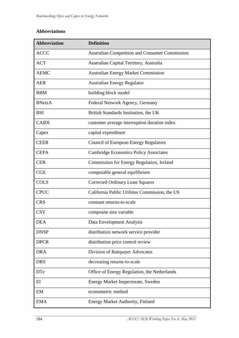
Benchmarking Opex and Capex in Energy Networks
ACCC/AER Working Paper No. 6, May 2012 184
Abbreviations
Abbreviation Definition
ACCC Australian Competition and Consumer Commission
ACT Australian Capital Territory, Australia
AEMC Australian Energy Market Commission
AER Australian Energy Regulator
BBM building block model
BNetzA Federal Network Agency, Germany
BSI British Standards Institution, the UK
CAIDI customer average interruption duration index
Capex capital expenditure
CEER Council of European Energy Regulators
CEPA Cambridge Economics Policy Associates
CER Commission for Energy Regulation, Ireland
CGE computable general equilibrium
COLS Corrected Ordinary Least Squares
CPUC California Public Utilities Commission, the US
CRS constant returns-to-scale
CSV composite size variable
DEA Data Envelopment Analysis
DNSP distribution network service provider
DPCR distribution price control review
DRA Division of Ratepayer Advocates
DRS decreasing returns-to-scale
DTe Office of Energy Regulation, the Netherlands
EI Energy Market Inspectorate, Sweden
EM econometric method
EMA Energy Market Authority, Finland
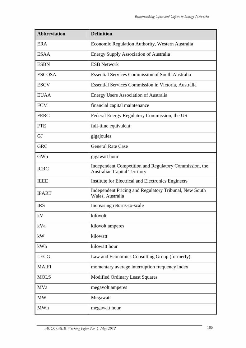
Benchmarking Opex and Capex in Energy Networks
ACCC/AER Working Paper No. 6, May 2012 185
Abbreviation Definition
ERA Economic Regulation Authority, Western Australia
ESAA Energy Supply Association of Australia
ESBN ESB Network
ESCOSA Essential Services Commission of South Australia
ESCV Essential Services Commission in Victoria, Australia
EUAA Energy Users Association of Australia
FCM financial capital maintenance
FERC Federal Energy Regulatory Commission, the US
FTE full-time equivalent
GJ gigajoules
GRC General Rate Case
GWh gigawatt hour
ICRC Independent Competition and Regulatory Commission, the
Australian Capital Territory
IEEE Institute for Electrical and Electronics Engineers
IPART Independent Pricing and Regulatory Tribunal, New South
Wales, Australia
IRS Increasing returns-to-scale
kV kilovolt
kVa kilovolt amperes
kW kilowatt
kWh kilowatt hour
LECG Law and Economics Consulting Group (formerly)
MAIFI momentary average interruption frequency index
MOLS Modified Ordinary Least Squares
MVa megavolt amperes
MW Megawatt
MWh megawatt hour
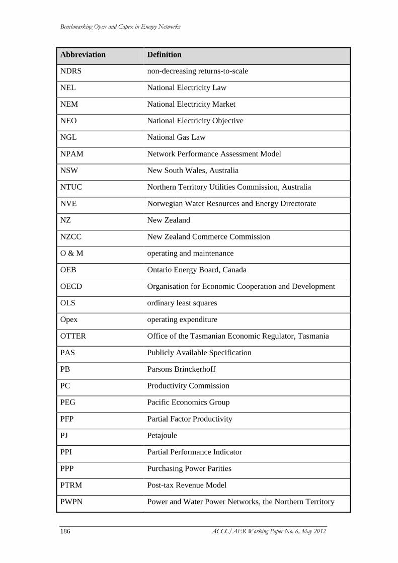
Benchmarking Opex and Capex in Energy Networks
ACCC/AER Working Paper No. 6, May 2012 186
Abbreviation Definition
NDRS non-decreasing returns-to-scale
NEL National Electricity Law
NEM National Electricity Market
NEO National Electricity Objective
NGL National Gas Law
NPAM Network Performance Assessment Model
NSW New South Wales, Australia
NTUC Northern Territory Utilities Commission, Australia
NVE Norwegian Water Resources and Energy Directorate
NZ New Zealand
NZCC New Zealand Commerce Commission
O & M operating and maintenance
OEB Ontario Energy Board, Canada
OECD Organisation for Economic Cooperation and Development
OLS ordinary least squares
Opex operating expenditure
OTTER Office of the Tasmanian Economic Regulator, Tasmania
PAS Publicly Available Specification
PB Parsons Brinckerhoff
PC Productivity Commission
PEG Pacific Economics Group
PFP Partial Factor Productivity
PJ Petajoule
PPI Partial Performance Indicator
PPP Purchasing Power Parities
PTRM Post-tax Revenue Model
PWPN Power and Water Power Networks, the Northern Territory
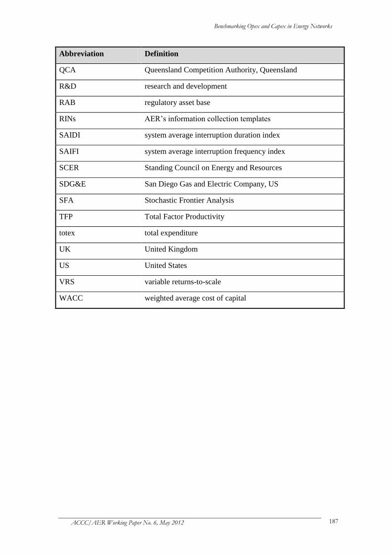
Benchmarking Opex and Capex in Energy Networks
ACCC/AER Working Paper No. 6, May 2012 187
Abbreviation Definition
QCA Queensland Competition Authority, Queensland
R&D research and development
RAB regulatory asset base
RINs AER’s information collection templates
SAIDI system average interruption duration index
SAIFI system average interruption frequency index
SCER Standing Council on Energy and Resources
SDG&E San Diego Gas and Electric Company, US
SFA Stochastic Frontier Analysis
TFP Total Factor Productivity
totex total expenditure
UK United Kingdom
US United States
VRS variable returns-to-scale
WACC weighted average cost of capital