A future perspective of historical contributionsto climate change

Ragnhild B. Skeie1 & Glen P. Peters1 & Jan Fuglestvedt1 & Robbie Andrew1

Received: 22 August 2019 /Accepted: 6 January 2021/# The Author(s) 2021

AbstractCountries’ historical contributions to climate change have been on the agenda for morethan two decades and will most likely continue to be an element in future internationaldiscussions and negotiations on climate. Previous studies have quantified the historicalcontributions to climate change across a range of choices and assumptions. In contrast,we quantify how historical contributions to changes in global mean surface temperature(GMST) may change in the future for a broad set of choices using the quantification ofthe shared socioeconomic pathways (SSPs). We calculate the contributions for five coarsegeographical regions used in the SSPs. Historical emissions of long-lived gases remainimportant for future contributions to warming, due to their accumulation and the inertia ofclimate system, and historical emissions are even more important for strong mitigationscenarios. When only accounting for future emissions, from 2015 to 2100, there issurprisingly little variation in the regional contributions to GMST change between thedifferent SSPs and different mitigation targets. The largest variability in the regionalfuture contributions is found across the different integrated assessment models (IAMs).This suggests the characteristics of the IAMs are more important for calculated futurehistorical contributions than variations across SSP or forcing target.

Keywords ParisAgreement .Historical contribution .Brazilianproposal . Shared socioeconomicpathways . Equity

1 Introduction

The Paris Agreement changed the role of historical responsibilities in international climatenegotiations (Skeie et al. 2017). Previously, the Kyoto Protocol was designed as a top-downagreement with a total cap on emissions for the Annex B countries. While it had been

https://doi.org/10.1007/s10584-021-02982-9

* Ragnhild B. Skeier.b.skeie@cicero.oslo.no

1 CICERO Center for International Climate Research, Pb. 1129 Blindern, 0318 Oslo, Norway

Published online: 28 January 2021

Climatic Change (2021) 164: 24

suggested to use historical contributions to global mean temperature change to distributeemission allocations to countries in the international climate agreement (the so-called “Brazil-ian proposal” (UNFCCC 1997)), it was found to be difficult to use in the internationalnegotiations (e.g., Fuglestvedt and Kallbekken 2016). The process leading to the ParisAgreement turned from designing a top-down agreement to a bottom-up agreement. Now,individual countries decide how much they are willing to reduce their emissions. Thenationally determined contributions (NDCs) are national pledges that contribute to meetingthe objectives of the United Nations Framework Convention on Climate Change (UNFCCC).With the Paris Agreement, historical responsibilities may again have a role to play: Accordingto the “Lima Call for Action” (UNFCCC 2014), NDCs should be fair and ambitious (Peterset al. 2015), but it is up to parties themselves to demonstrate this, leaving open the potential useof historical contribution as an argument on the international stage and also as an element incountries’ domestic discussions of negotiating positions and ambitions. Because countries arerequired to submit revised national contributions every 5 years, historical contribution toclimate change may become even more relevant in the future. Consideration of historicalcontribution is also likely to play a key role in the future discussions about loss and damage(James et al. 2019; Otto et al. 2017; Skeie et al. 2017).

Relative regional and national historical contributions to global warming have changedconsiderably over recent decades. Estimated shares of historical contributions were quitedifferent when “historical responsibilities” were first put on the agenda in 1997 than theyare today. When considering CO2 emissions from fossil sources from 1850, the historicalcontribution in 1997 was 76% for the Annex I countries, while in 2012, this share had declinedto 68% (Skeie et al. 2017). There has been a rapid increase in emissions in developingcountries over the past decades (Le Quéré et al. 2018), and the regional share of totalgreenhouse gas emission will change in the near future due to the differences in the trajectoriesof income, population, resources, technologies, and capacity (Riahi et al. 2017), leading also tochanged historical contributions to global warming in the future (Höhne et al. 2011; Rive et al.2006; Ward and Mahowald 2014).

A number of studies have focused on regional historical contribution to global warming forvarious assumptions using simple or more complex models (den Elzen et al. 2005; den Elzenet al. 2013; Höhne et al. 2011; Li et al. 2016; Matthews et al. 2014; Ward and Mahowald 2014;Wei et al. 2012). A recent study by Skeie et al. (2017) showed systematically that differentadopted perspectives had a strong effect on the calculated historical contribution to globalwarming. Here, we take a step further and illustrate, for different perspectives, how thecontributions to global mean surface temperature change may change over the coming decadesand discuss other perspectives that may need to be considered. The traditional method toallocate emissions to countries is allocating the emissions occurring within the country’sborders. Future flexible mechanisms and emission trading may challenge the use of traditionalterritorial accounting when assessing contribution to climate change, as well as carbon dioxideremoval (Peters and Geden 2017). How should carbon dioxide removal be allocated betweenthe countries involved from biomass growth, harvest, energy production and CO2 capture, andeventual storage? For the flexible mechanisms, should the emission reduction be allocated tothe country buying quotas or to the country where the emission reduction occurs?

To illustrate potential future historical contributions to global temperature change, we usethe shared socioeconomic pathways (SSPs) (Riahi et al. 2017) and a simple climate model(Skeie et al. 2017). The quantified SSPs are grouped into five geographical regions, allowingthe analysis of how future historical contributions are distributed across those regions. Further,

Climatic Change (2021) 164: 2424 Page 2 of 13

the SSPs span five socioeconomic pathways, six levels of global warming, and six integratedassessment models (IAMs), allowing a deeper analysis of how historical contributions dependon these different dimensions.

2 Method

We follow the method used in Skeie et al. (2017), using a simple climate model andemission inventories to calculate regional contributions to global mean surface temper-ature (GMST) change. The results are presented as relative contribution to GMSTchange, where the total is the sum of each individual region contribution to GMSTchange. In addition to historical emission inventories, we use SSPs to illustrate anddiscuss the future perspective of historical contribution to global warming (Fig. 1). Amain point in Skeie et al. (2017) was that various scientific and policy choices influencethe calculations of historical contributions for individual countries, and Skeie et al.(2017) quantified the effects of different choices. In this study, we limit our analysis tothree different start years (1850: pre-industrial, 1992: UN Framework Convention onClimate Change (UNFCCC), and 2015: the Paris Agreement) and two sets of components(CO2FF: CO2 from fossil fuel combustion and cement production and KP: KyotoProtocol gases, which in principle means CO2FF, CO2 from land-use change (LUC),CH4 and N2O as the impacts of SF6, PFC and HFCs on calculated relative contributionsare negligible (Skeie et al. 2017)) using regional territorial-based emissions and GMSTas indicators of climate change. There are several other methodological choices that canbe made that will influence the results (Skeie et al. 2017); however, to make the analysistractable, we focus on a limited number of key dimensions.

Fig. 1 Schematic overview of the setup of the simulation. The regional historical and future emissionsconsidered are grouped into two sets of components, CO2FF and KP. A wide range of future scenarios isconsidered, generated by different IAMs, considering different SSPs and with different mitigation targets. Thecalculations of relative contribution to global mean surface temperature change are performed with different startyears and results presented for different evaluation years. The historical relative contributions to global meansurface temperature change are calculated based on the traditional territorial-based emissions, but emissiontrading might confound the traditional territorial emission accounting. The five regions considered in this studyare indicated by colors and abbreviation in the map. The regions are the OECD, countries from the ReformingEconomies of Eastern Europe and the Former Soviet Union (REF), ASIA, the Middle East and Africa (MAF),and Latin America and the Caribbean (LAM)

Climatic Change (2021) 164: 24 Page 3 of 13 24

2.1 Model

The CICERO Simple climate model (SCM) consists of an energy balance/upwelling diffusionmodel (Schlesinger et al. 1992) and a carbon cycle model (Joos et al. 1996) as well as simplifiedcalculations from emissions via concentrations or directly to forcing. A detailed description of themodel is presented by Skeie et al. (2017). A recent study showed that methane forcing issignificantly stronger than previously thought (Etminan et al. 2016), and new expressions of CO2,CH4, and N2O radiative forcing presented in that study are now implemented in the SCM. For CO2

and N2O, the change is minimal; however, for methane, the revision is significant, with 25%stronger forcing than presented in the IPCC Fifth Assessment Report (Myhre et al. 2013). Theindirect aerosol forcing is now linearly scaled with SO2 emissions, as studies indicate that the totalglobal effect is linear (Kretzschmar et al. 2017) rather than logarithmic as previously specified in themodel. A set of model parameters with an inferred effective climate sensitivity of 2.0 °C and thecorresponding aerosol forcing from Skeie et al. (2018) is used. Because the main focus of this studyis changes in the relative contribution toGMST change, uncertainties inmodel version are of limitedimportance due to cancelations of the climate system response uncertainties when relative contri-butions are calculated.

2.2 Setup

The future emissions scenarios used in this study are from the SSP V2.0 database (https://tntcat.iiasa.ac.at/SspDb/dsd?Action=htmlpage&page=about) (Riahi et al. 2017). These scenar-ios are available for the following five geographical regions: OECD (defined as the OECDmembers in 1990 and EU member states and candidates), REF (countries from the ReformingEconomies of Eastern Europe and the Former Soviet Union), ASIA (most Asian countries withthe exception of the Middle East, Japan, and Former Soviet Union states), MAF (the MiddleEast and Africa), and LAM (Latin America and the Caribbean) (Fig. 1). We could not performthe analysis at the country level since scenario emissions are not available at this level.

There are in total 127 scenarios grouped into six radiative forcing levels (FLs) or mitigationtargets (FL1.9: 1.9Wm−2, FL2.6: 2.6Wm−2, FL3.4: 3.4Wm−2, FL4.5: 4.5Wm−2, FL6.0: 6.0Wm−2,and BASELINE) as well as five shared socioeconomic pathways (SSPs). We use the term “forcinglevels” as in the literature (O'Neill et al. 2016; Riahi et al. 2017) to distinguish from the specificrepresentative concentration pathways (RCPs) as used in the IPCC Fifth Assessment Report. Thefive pathways are SSP1: sustainability, SSP2: middle of the road, SSP3: regional rivalry, SSP4:inequality, and SSP5: rapid growth (O’Neill et al. 2014). Each SSP and forcing level has beenimplemented across multiple IAMs.With six IAMs, six FLs, and five SSPs, there are in theory 180scenarios, but not all IAMs tried every SSP and FL combination and some IAMs were unable tomeet the highest and lowest forcing levels for some SSPs (Rogelj et al. 2018). In total, there are 127scenarios distributed across different forcing levels: FL1.9: 13, FL2.6: 19, FL3.4: 25, FL4.5: 25,FL6.0: 19, and BASELINE: 26. The results from calculations of contributions are presentedaccording to the (i) forcing level, (ii) SSP, and (iii) IAM used to generate the scenario emissions.

Two sets of components are included; only CO2 fossil fuel and the group of the mainKyoto Protocol components total CO2, N2O, and CH4. Short-lived components includingaerosols are not included to make the analysis more tractable. Our previous study showedthat the relative contributions from the different countries did not change strongly fromthe Kyoto Protocol component results if short-lived warming and cooling componentswere included (Skeie et al. 2017).

Climatic Change (2021) 164: 2424 Page 4 of 13

To calculate the climate impact of each region, we first run the SCM with all anthropogenicemissions included and then run the SCM with emissions from each region removed one-by-one, and the change in GMST is calculated as the difference between global (control) andregional (perturbed) run. There are different approaches to account for the non-linearities in theclimate response as discussed in Trudinger and Enting (2005), and here, the emissionperturbations are scaled down to 10%. The relative contribution to GMST change is givenin relation to the sum of each individual region’s contribution to GMST change; hence, thecontribution from all regions adds to 100%. The background scenarios used in the SCM for thecontrol are one of the four RCPs (van Vuuren et al. 2011), chosen based on the total forcing in2100 for each of the SSP scenarios: RCP2.6: < 3.6 Wm−2, RCP4.5: 3.6 to 5.2 Wm−2, RCP6.0:5.2 to 7.3 Wm−2, and RCP8.5: > 7.3 Wm−2.

In this study, we have chosen to use three different start years: 1850, 1992, and 2015(corresponding to pre-industrial period, signing of UNFCCC, and the Paris Agreement). Themodel is run with emission perturbation from the start year until 2100 and we focus on fiveevaluation years, 1992, 2015, 2030, 2065, and 2100.

The historical emissions used in this study are from Le Quéré et al. (2018) for CO2

(fossil fuels and cement), Hoesly et al. (2018) for methane, and EDGARv432 (Janssens-Maenhout et al. 2019) from 1970 to 2012 scaled backward using emission data fromMATCH (Höhne et al. 2011) for N2O. Historical emissions for CO2 from land-usechange are taken from Houghton and Nassikas (2017). There are uncertainties in thehistorical emission estimates, especially for CO2 emissions from land-use change (LeQuéré et al. 2018). This will especially influence results using 1850 as start year whenland-use change emissions are included. Results using 1992 as start year are obviouslyless influenced by historical emissions, and 2015 as start year uses only (future) scenariodata. The focus of this paper is on the future developments and contributions, but we areaware of the uncertainties in the historical emissions and their impacts on the calculatedregional relative contributions for early start years. The historical emissions are aggre-gated to the five chosen regions.

The regional emissions in the last year of the historical inventory generally do not match thescenario emissions for the same year. The differences between the historical inventory and thescenario emissions are as follows: (1) different historical emission inventories are generallyused by each IAM and (2) the scenarios are often started in 2010 or 2015 and thus divergefrom historical emissions, which are up to a more recent year. It should also be noted thatuncertainties in the current anthropogenic emissions of CH4 and N2O are substantial (Saunoiset al. 2020; Tian et al. 2020), particularly for land-use-related CO2 emissions (Friedlingsteinet al. 2019). We have chosen to linearly interpolate the regional emissions between the endyear of the historical inventory (N2O: 2012, CH4: 2014, CO2 FF: 2017, CO2 LUC: 2015) andyear 2020 of the scenario (see supporting Fig. S1–S4) as our focus is future contribution towarming and we want to avoid unnecessarily manipulating the original scenarios. Othermethods to harmonize historical emissions and scenarios exist (Gidden et al. 2018; Rogeljet al. 2011). Different methods of harmonization will lead to slightly different results, but sincewe focus on the future period (post-2015), this issue is minimized. The most problematicvariable is CO2 LUC, where the regional emissions can even have the opposite sign to thehistorical emissions in some scenarios (see supporting Fig. S5). A reasonable transition fromthe historical regional emissions to the scenario emissions is hence difficult, and for thisreason, no harmonization on a regional scale is performed for CO2 LUC in the Coupled ModelIntercomparison Project Phase 6 (Gidden et al. 2019).

Climatic Change (2021) 164: 24 Page 5 of 13 24

3 Results

Wewill first consider the effect on the calculated relative contribution to GMST change for thechoice of different evaluation years for the two sets of emission components (Fig. 2). Then, forthe same set of emission components, the impact of the choice of start year is illustrated(Fig. 3). Further, the regional historical contribution (pre-2015) and the future contribution(post-2015) to GMST change in 2100 are compared across all mitigation targets and SSPs(Fig. 4). Finally, we will explore and compare the effects of SSPs, mitigation targets, andIAMs on the regional relative contribution to GMST change in 2100 (Fig. 5).

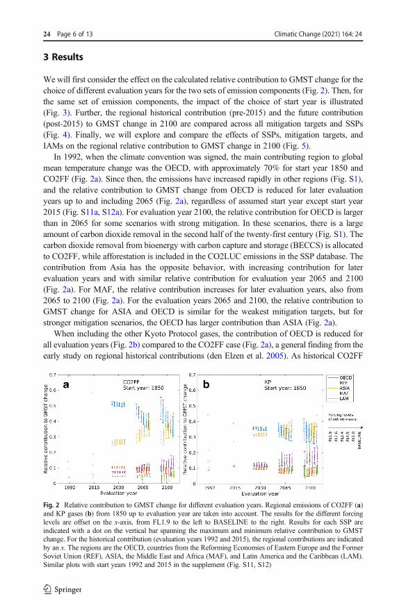
In 1992, when the climate convention was signed, the main contributing region to globalmean temperature change was the OECD, with approximately 70% for start year 1850 andCO2FF (Fig. 2a). Since then, the emissions have increased rapidly in other regions (Fig. S1),and the relative contribution to GMST change from OECD is reduced for later evaluationyears up to and including 2065 (Fig. 2a), regardless of assumed start year except start year2015 (Fig. S11a, S12a). For evaluation year 2100, the relative contribution for OECD is largerthan in 2065 for some scenarios with strong mitigation. In these scenarios, there is a largeamount of carbon dioxide removal in the second half of the twenty-first century (Fig. S1). Thecarbon dioxide removal from bioenergy with carbon capture and storage (BECCS) is allocatedto CO2FF, while afforestation is included in the CO2LUC emissions in the SSP database. Thecontribution from Asia has the opposite behavior, with increasing contribution for laterevaluation years and with similar relative contribution for evaluation year 2065 and 2100(Fig. 2a). For MAF, the relative contribution increases for later evaluation years, also from2065 to 2100 (Fig. 2a). For the evaluation years 2065 and 2100, the relative contribution toGMST change for ASIA and OECD is similar for the weakest mitigation targets, but forstronger mitigation scenarios, the OECD has larger contribution than ASIA (Fig. 2a).

When including the other Kyoto Protocol gases, the contribution of OECD is reduced forall evaluation years (Fig. 2b) compared to the CO2FF case (Fig. 2a), a general finding from theearly study on regional historical contributions (den Elzen et al. 2005). As historical CO2FF

Fig. 2 Relative contribution to GMST change for different evaluation years. Regional emissions of CO2FF (a)and KP gases (b) from 1850 up to evaluation year are taken into account. The results for the different forcinglevels are offset on the x-axis, from FL1.9 to the left to BASELINE to the right. Results for each SSP areindicated with a dot on the vertical bar spanning the maximum and minimum relative contribution to GMSTchange. For the historical contribution (evaluation years 1992 and 2015), the regional contributions are indicatedby an x. The regions are the OECD, countries from the Reforming Economies of Eastern Europe and the FormerSoviet Union (REF), ASIA, the Middle East and Africa (MAF), and Latin America and the Caribbean (LAM).Similar plots with start years 1992 and 2015 in the supplement (Fig. S11, S12)

Climatic Change (2021) 164: 2424 Page 6 of 13

emissions were dominated by OECD (Fig. S1), the regional distribution of the other emissionsis more mixed (Fig. S2–S4). For 2030, the OECD contribution to GMST change is slightlylarger than the contribution from ASIA, while ASIA is similar or larger for later evaluationyears for all forcing targets (Fig. 2b). The contributions from LAM and MAF increase whenincluding the other Kyoto Protocol gases, and both regions have a larger historical contributionthan REF for the evaluation year 2030 for all scenarios, while in the CO2FF case, REF had thelargest contribution of these three regions (Fig. 2a). It should be noted that the results for 2030are influenced by methods used to harmonize the scenario emissions and the historicalinventory. Here, we have chosen to keep the original scenario emissions post-2020 (seeSection 2.2). If a uniform scaling harmonization is applied (that scales the entire pathway tomatch the historical emission), the spread in the results is reduced (Fig. S6). This test is onlypreformed for CO2FF as a reasonable transition from the historical inventory to the scenario isdifficult for CO2 LUC (see Section 2.2).

Figure 3 shows how the regional contributions to GMST change in 2100 depend on thestart year (1850, 1992, 2015). For CO2FF, the earlier the start year, the smaller the contributionfrom ASIA and the larger the contribution from OECD (Fig. 3a), as OECD dominated thehistorical CO2FF emissions while ASIA currently has the largest CO2FF emissions (Fig. S1).The effect of larger contribution from developed countries for earlier start year is expected andfound in previous studies (den Elzen et al. 2005; Höhne et al. 2011; Skeie et al. 2017). Thecontribution from MAF increases with a later start year, while REF and LAM have similarcontributions for different start years. In the strongest mitigation scenario (FL1.9), scenariosmake use of large-scale carbon dioxide removal (primarily afforestation and BECCS). Inseveral of the scenarios, there are regions that contribute to cooling, with negative cumulativeCO2FF emissions over the evaluation period. For these regions, we set the contribution to zerowarming effect when calculating the relative contribution, implying that the regions with apositive contribution will have a larger relative contribution. Also, in the mitigation levelsFL2.6 and FL3.4, there are a few scenarios where LAM and REF contribute to cooling. Forstart year 1850, the relative contribution to GMST change in 2100 is dependent on themitigation target, for all regions except REF. For a strong mitigation target, there is less room

Fig. 3 Impacts of start year of emissions on the regional contribution to GMST change in 2100 for the CO2FFcase (a) and Kyoto Protocol gases case (b). The results for the different forcing targets are shifted on the x-axis,from FL1.9 to the left to BASELINE to the right. Results for each SSP are indicated with a dot. Regionscontributing to cooling are set to zero in the plot and when relative contributions are calculated. The regions arethe OECD, countries from the Reforming Economies of Eastern Europe and the Former Soviet Union (REF),ASIA, the Middle East and Africa (MAF), and Latin America and the Caribbean (LAM)

Climatic Change (2021) 164: 24 Page 7 of 13 24

for future emissions, and the relative contributions are therefore more dependent on thehistorical emissions. For weaker mitigation targets, the future emissions, with a differentregional distribution than the historical emissions (Fig. S1), hold a larger share of the totalcumulative emissions and hence influence the relative contribution in 2100 to a larger degreethan for the strong mitigation targets. For a late start year, there is less variability on relativecontributions between the mitigation targets, indicating relative mitigation contributions aresimilar across regions, perhaps because IAMs often seek cost-effective mitigation pathways.

Looking at the case including the Kyoto Protocol gases (Fig. 3b), compared to CO2FF (Fig.3a), the contribution from OECD is reduced. The contribution from MAF and LAM isincreased due to the higher share of methane and land-use change CO2 emissions from thesetwo regions compared to the other regions (Fig. S2–S3). Compared to the CO2FF case, there isless variation across the chosen start years, because of different temporal development of CO2

LUC emissions (Fig. S2) and inclusion of methane with its shorter lifetime, and therefore,there is no influence on the temperature response in 2100 for the early emissions. For start year2015 (at the time of the Paris Agreement), the relative contribution to GMST change fromMAF overlaps with the contribution from the OECD for the evaluation year 2100 for most ofthe scenarios, compared to almost no overlap if only CO2FF is included (Fig. 3a) exceptforcing target FL1.9.

In order to compare the historical contributions from 1850 to 2015 to the contributions from2015 to 2100 to the temperature response in 2100, an additional set of simulations isperformed, where the temperature response in 2100 is calculated due to the regional emissionsfor the years 1850 to 2015. This set of simulations is combined with simulations with start year2015, so that the historical contributions in 2100 can be split into two, the contribution from1850 to 2015 and 2015 to 2100. The results for the KP case are presented in Fig. 4 wherehistorical (darker colors) and future contribution (lighter colors) for each region to thetemperature change in 2100 are shown. A pie chart is shown for each set of mitigation targetsand SSPs. As expected, the stronger the mitigation target, the smaller the contribution of 2015–2100 emissions to temperature change in 2100. For strong mitigation (e.g., FL2.6), historicalOECD emissions have the largest share of contribution to GMST change in 2100 (22%), whilethe share is reduced to 7 to 12% (depending on SSP) for BASELINE. For weak mitigation(BASELINE), the contribution from post-2015 emissions from ASIA has the largest share ofGMST change in 2100 (31 to 34% depending on SSP). Regardless of SSP or forcing level,ASIA andMAF have a much larger contribution from 2015 compared to before 2015. ASIA isthe region with largest emissions in 2015 (Fig. S1–S4) for all components considered exceptCO2 LUC, and it is assumed to continue to be the regions with the largest emissions over thenext decades in the scenarios. ASIA’s CO2FF emissions have increased rapidly over the lastdecades (Fig. S1), and hence, the region has a small share of the historical global emissionswhen compared with its current share. Currently, MAF has a small share of the historicalemissions, but in all scenarios, a strong increase in both population and GDP growth isassumed (Fig. S7–S8), giving a larger share of post-2015 emissions compared to pre-2015in all scenarios. The other three regions, OECD, REF, and LAM, have a more equalcontribution before and after 2015, but with a larger share of pre-2015 emissions for strongmitigation and larger share of post-2015 emissions for weak mitigation.

Notable changes in the regional contributions across forcing target for each SSP are seen,especially when the regional contributions are split into post- and pre-2015 contributions (Fig.4, across the rows). However, for a given mitigation target, there is no clear pattern of changein the regional contribution for the different SSPs (Fig. 4, down the columns). We will now

Climatic Change (2021) 164: 2424 Page 8 of 13

investigate the surprisingly little difference in regional variations across the SSPs. As we sawin Fig. 3, there was also little variability in the relative contributions between the mitigationtargets for late start year, which indicated the models produce similar relative mitigation levelsacross regions. To remove the influence and inertia from the earlier historical period up until2015, we focus on the regional contribution to GMST change in 2100 for emissions occurringin the period 2015 to 2100. We add a third dimension when presenting the results, the IAMsused to generate the scenario emissions.

The results for KP are presented in three different ways, including the three dimensionsSSPs, forcing levels, and IAMs (Fig. 5). A first observation is that there is no clear or obvioustrend in any of the three dimensions. This suggests that the SSPs do not have sufficient detailto differentiate historical contribution for these geographical regions, though SSP3 shows amore distinct difference in the regional contribution from ASIA and OECD. For example,SSP1 and SSP5 have lower inequality compared to SSP3 and SSP4, but this does not translateto macrolevel differences in how the regions may develop or implicitly allocate mitigationobligations. The similar variations across forcing targets indicate that mitigation follows the

Fig. 4 Relative contribution to GMST change in 2100 from different regions and time periods for KP. Darkcolors indicate regional contribution due to emissions in the period 1850 to 2015, while lighter colors indicateregional contribution due to emissions over the period 2015 to 2100. Contributions are plotted for each mitigationand SSP. The median temperature response in 2100 is used for this figure. The regions are the OECD, countriesfrom the Reforming Economies of Eastern Europe and the Former Soviet Union (REF), ASIA, the Middle Eastand Africa (MAF), and Latin America and the Caribbean (LAM). A similar figure for CO2FF in the supplement(Fig. S9)

Climatic Change (2021) 164: 24 Page 9 of 13 24

same allocation rules, regardless of SSP or IAM. Since the same distribution occurs underreference and deep mitigation scenarios, and across SSPs, it may indicate that the cost-effective mitigation in IAMs is essentially equivalent to grandfathering (allocating accordingto the current distribution of emissions).

While the SSPs are designed to include aspects of inequality, that does not translate intohistorical contributions. There are two key reasons for this. First, the SSPs apply to the wholeworld, and different SSPs are not mixed across regions. For example, in an SSP3 RegionalRivalry world, all regions have the same assumptions, likewise for all other SSPs. Second,IAMs are solved in a cost-optimizing way, meaning they reduce emissions where it ischeapest. While some of the SSPs introduce climate policy at a different rate (Riahi et al.2017), this fragmentation quickly dissipates by 2040. Effectively, the SSPs were not designedspecifically to introduce equity dimensions into stringent mitigation, and thus, it would not beexpected that a large variation occurs in historical responsibility for a given SSP with no,weak, or strong mitigation. It should be noted that not all IAMs were able to resolve some ofthe lowest forcing levels for all SSPs (Rogelj et al. 2018), meaning there may be differentmodels in each SSP-FL subgroup. However, we do not see a variation between the SSPs athigher forcing levels either where all models are included, suggesting that scenario bias acrossIAMs or SSPs is not a factor.

The most significant difference across the three dimensions seems to be the IAMs,indicating that the IAM used to generate emissions pathways is more important for calculatedfuture contributions than the SSP or forcing target. When holding the IAM constant (Fig. 5c),it also reveals more structure across SSP and forcing target. AIM/GGE and REMIND clearlylead to lower contributions from ASIA; IMAGE has a lower contribution for OECD and alarger contribution from LAM andWITCH and a lower contribution for MAF compared to theother IAMs. GCAM clearly shows variation across forcing target for REF and LAM, and

Fig. 5 Relative contribution to GMST change in 2100 for regional emissions of Kyoto Protocol gases with startyear 2015. The results are presented in three different ways, with SSPs on the x-axis with minor offset on the x-axis for the forcing targets (a), with forcing targets on the x-axis with minor shift on the x-axis for the SSPs (b),and with IAMs on the x-axis and minor shift in the x-axis for the SSPs (c). The regions are the OECD, countriesfrom the Reforming Economies of Eastern Europe and the Former Soviet Union (REF), ASIA, the Middle Eastand Africa (MAF), and Latin America and the Caribbean (LAM). A similar figure for regional emissions ofCO2FF in the supplement (Fig. S10)

Climatic Change (2021) 164: 2424 Page 10 of 13

MESSAGE for LAM, with larger contributions for larger forcing targets. GCAM has lowercontribution for ASIA with SSP4 and significantly higher contribution for MAF compared tothe rest of the SSPs. A closer inspection across the IAMs reveals different sub-patterns acrossSSPs and forcing levels. Within each of the IAMs, there may be particular aspects that drivethese patterns, but it is beyond the scope of this paper to be able to analyze those aspects.

4 Conclusion

We estimated the future contributions to GMST change using emission scenarios spanning fivegeographical regions, five shared socioeconomic pathways (SSPs), six radiative forcing levels,and six IAMs and investigated causes of variations across these selections.We find that the period1850 to 2015 is important for future contributions, due to the inertia effects of long-livedgreenhouse gases accumulating in the atmosphere (CO2 and N2O), and increasingly moreimportant for strongmitigation scenarios (e.g., 1.5 and 2 °C) due to less room for future emissions.Since the SSPs incorporate a broad range of socioeconomic characteristics that affect thechallenges to mitigation and adaptation, it could be expected that the future contributions varyby SSP. We found that from 2015 to 2100, there is surprisingly little variation across SSPs andforcing levels to the regional contributions to GMST change. This suggests that mitigation occursat similar rates in the different regions for a given mitigation scenario, which is expected as aconsequence of the cost-effective pathways followed in most IAMs (mitigation occurs where it ischeapest). If the scenarios were set up with a stronger equity dimension, for example, by havingmuch earlier and deeper mitigation in wealthier countries, then more variations may be seen. Thecalculations were performed for five large geographical regions, and it may be that much morevariation would be found at a disaggregated level. Larger variations are found across IAMs, butthe pattern varies across IAMs for SSP and forcing targets. This indicates that the choice of IAM ismore important for calculated future contributions than either SSP or forcing target.

We considered emission scenarios for five large geographical regions to illustrate futurehistorical contributions to GMST change. On a more detailed country level, additionalcomplications may arise. First, contributions based on the traditional accounting of territorialemissions may become complicated in the future if flexibility mechanisms are increasinglyused. The Paris Agreement has provisions for the use of flexibility mechanisms (e.g., emissiontrading), but it still remains unclear as to what extent the flexibility mechanisms will be used inthe future (UNFCCC 2018). Second, most mitigation scenarios use carbon dioxide removal(particularly afforestation and BECCS), and at the regional and country level, this eventuallyleads to negative contributions to climate change. Particularly at the detailed country level,how to deal with carbon dioxide removal may lead to additional allocation challenges.

The scenarios we used span a range of possible futures up to 2100, and we have used theseto illustrate future regional contributions to climate change. Although the countries havesubmitted NDCs, we do not know if they will be fulfilled or what role flexible mechanismsmay play. Countries have only specified commitments until 2025 or 2030 (Gütschow et al.2018), but the NDCs can be strengthened and will eventually be extended post-2030. TheNDCs are required to be fair and ambitious (Peters et al. 2015), and historical contributionscould play a role in helping to assess if an NDC is fair and ambitious. The politicallycontentious issue of countries’ historical contributions to climate change will no doubt bebrought on the agenda in the future, both when countries strengthen their NDCs and possiblyin loss and damage discussions.

Climatic Change (2021) 164: 24 Page 11 of 13 24

Supplementary Information The online version contains supplementary material available at https://doi.org/10.1007/s10584-021-02982-9.

Acknowledgments This work was funded by the Norwegian Ministry of Foreign Affairs.

Open Access This article is licensed under a Creative Commons Attribution 4.0 International License, whichpermits use, sharing, adaptation, distribution and reproduction in any medium or format, as long as you giveappropriate credit to the original author(s) and the source, provide a link to the Creative Commons licence, andindicate if changes were made. The images or other third party material in this article are included in the article'sCreative Commons licence, unless indicated otherwise in a credit line to the material. If material is not includedin the article's Creative Commons licence and your intended use is not permitted by statutory regulation orexceeds the permitted use, you will need to obtain permission directly from the copyright holder. To view a copyof this licence, visit http://creativecommons.org/licenses/by/4.0/.

References

den Elzen M et al (2005) Analysing countries’ contribution to climate change: scientific and policy-relatedchoices. Environ Sci Pol 8:614–636. https://doi.org/10.1016/j.envsci.2005.06.007

den Elzen MJ, Olivier JJ, Höhne N, Janssens-Maenhout G (2013) Countries’ contributions to climate change:effect of accounting for all greenhouse gases, recent trends, basic needs and technological progress. ClimChang 121:397–412. https://doi.org/10.1007/s10584-013-0865-6

EtminanM, Myhre G, Highwood EJ, Shine KP (2016) Radiative forcing of carbon dioxide, methane, and nitrousoxide: a significant revision of the methane radiative forcing. Geophys Res Lett 43:12,614–612,623. https://doi.org/10.1002/2016GL071930

Friedlingstein P et al (2019) Global Carbon Budget 2019. Earth Syst Sci Data 11:1783–1838. https://doi.org/10.5194/essd-11-1783-2019

Fuglestvedt JS, Kallbekken S (2016) Climate responsibility: fair shares? Nat Clim Chang 6:19–20. https://doi.org/10.1038/nclimate2791

Gidden MJ, Fujimori S, van den Berg M, Klein D, Smith SJ, van Vuuren DP (2018) Riahi K, A methodologyand implementation of automated emissions harmonization for use in integrated assessment models envi-ronmental modelling & software. 105:187–200. https://doi.org/10.1016/j.envsoft.2018.04.002

Gidden MJ et al (2019) Global emissions pathways under different socioeconomic scenarios for use in CMIP6: adataset of harmonized emissions trajectories through the end of the century. Geosci Model Dev 12:1443–1475. https://doi.org/10.5194/gmd-12-1443-2019

Gütschow J, Jeffery ML, Schaeffer M, Hare B (2018) Extending near-term emissions scenarios to assess warmingimplications of Paris Agreement NDCs Earth’s future. 6:1242–1259. https://doi.org/10.1002/2017EF000781

Hoesly RM et al (2018) Historical (1750–2014) anthropogenic emissions of reactive gases and aerosols from theCommunity Emissions Data System (CEDS). Geosci Model Dev 11:369–408. https://doi.org/10.5194/gmd-11-369-2018

Höhne N et al (2011) Contributions of individual countries’ emissions to climate change and their uncertainty.Clim Chang 106:359–391. https://doi.org/10.1007/s10584-010-9930-6

Houghton RA, Nassikas AA (2017) Global and regional fluxes of carbon from land use and land cover change1850–2015. Global Biogeochem Cy 31:456–472. https://doi.org/10.1002/2016GB005546

James RA, Jones RG, Boyd E, Young HR, Otto FEL, Huggel C, Fuglestvedt JS (2019) Attribution: how is itrelevant for loss and damage policy and practice? In: Mechler R. BL, Schinko T., Surminski S., Linnerooth-Bayer J. (ed) Loss and damage from climate change. Climate risk management, policy and governance.Springer, Cham

Janssens-Maenhout G et al (2019) EDGAR v4.3.2 Global Atlas of the three major greenhouse gas emissions forthe period 1970–2012. Earth Syst Sci Data 11:959–1002. https://doi.org/10.5194/essd-11-959-2019

Joos F, Bruno M, Fink R, Siegenthaler U, Stocker TF, Lequere C (1996) An efficient and accurate representationof complex oceanic and biospheric models of anthropogenic carbon uptake. Tellus B 48:397–417

Kretzschmar J, Salzmann M, Mülmenstädt J, Boucher O, Quaas J (2017) Comment on “rethinking the lowerbound on aerosol radiative forcing”. J Clim 30:6579–6584. https://doi.org/10.1175/JCLI-D-16-0668.1

Le Quéré C et al (2018) Global Carbon Budget 2018. Earth Syst Sci Data 10:2141–2194. https://doi.org/10.5194/essd-10-2141-2018

Climatic Change (2021) 164: 2424 Page 12 of 13

LiB et al (2016) The contribution ofChina’s emissions to global climate forcing.Nature 531:357–361. https://doi.org/10.1038/nature17165 http://www.nature.com/nature/journal/v531/n7594/abs/nature17165.html#supplementary-information

Matthews HD, Tanya LG, Serge K, Cassandra L, Donny S, Trevor JS (2014) National contributions to observedglobal warming. Environ Res Lett 9:014010

Myhre G et al (2013) Anthropogenic and natural radiative forcing. In: Stocker TF et al (eds) Climate change2013: the physical science basis. Contribution of Working Group I to the Fifth Assessment Report of theIntergovernmental Panel on Climate Change. Cambridge University Press, Cambridge, United Kingdom andNew York, NY, USA

O’Neill BC et al (2014) A new scenario framework for climate change research: the concept of sharedsocioeconomic pathways. Clim Chang 122:387–400. https://doi.org/10.1007/s10584-013-0905-2

O'Neill BC et al (2016) The Scenario Model Intercomparison Project (ScenarioMIP) for CMIP6. Geosci ModelDev 9:3461–3482. https://doi.org/10.5194/gmd-9-3461-2016

Otto FEL, Skeie RB, Fuglestvedt JS, Berntsen T, Allen MR (2017) Assigning historic responsibility for extremeweather events. Nat Clim Chang 7:757. https://doi.org/10.1038/nclimate3419

Peters GP, Geden O (2017) Catalysing a political shift from low to negative carbon. Nat Clim Chang 7:619.https://doi.org/10.1038/nclimate3369

Peters GP, Andrew RM, Solomon S, Friedlingstein P (2015) Measuring a fair and ambitious climate agreementusing cumulative emissions. Environ Res Lett 10:105004. https://doi.org/10.1088/1748-9326/10/10/105004

Riahi K et al (2017) The shared socioeconomic pathways and their energy, land use, and greenhouse gas emissionsimplications: an overview. Glob Environ Chang 42:153–168. https://doi.org/10.1016/j.gloenvcha.2016.05.009

Rive N, Torvanger A, Fuglestvedt JS (2006) Climate agreements based on responsibility for global warming:periodic updating, policy choices, and regional costs. Glob Environ Chang 16:182–194. https://doi.org/10.1016/j.gloenvcha.2006.01.002

Rogelj J, Hare W, Chen C, Meinshausen M (2011) Discrepancies in historical emissions point to a wider 2020gap between 2 °C benchmarks and aggregated national mitigation pledges. Environ Res Lett 6:024002.https://doi.org/10.1088/1748-9326/6/2/024002

Rogelj J et al (2018) Scenarios towards limiting global mean temperature increase below 1.5 °C. Nat Clim Chang8:325–332. https://doi.org/10.1038/s41558-018-0091-3

Saunois M et al (2020) The Global Methane Budget 2000–2017. Earth Syst Sci Data 12:1561–1623. https://doi.org/10.5194/essd-12-1561-2020

Schlesinger ME, Jiang X, Charlson RJ (1992) Implication of anthropogenic atmospheric sulphate for thesensitivity of the climate system. In: Rosen L, Glasser R (eds) Climate change and energy policy:Proceedings of the International Conference on Global Climate Change: its mitigation through improvedproduction and use of energy. American Institute of Physics, New York, pp 75–108

Skeie RB, Fuglestvedt J, Berntsen T, Peters GP, Andrew R, Allen M, Kallbekken S (2017) Perspective has astrong effect on the calculation of historical contributions to global warming. Environ Res Lett 12:024022

Skeie RB, Berntsen T, Aldrin M, Holden M, Myhre G (2018) Climate sensitivity estimates – sensitivity to radiativeforcing time series and observational data. Earth Syst Dynam 9:879–894. https://doi.org/10.5194/esd-9-879-2018

Tian H et al (2020) A comprehensive quantification of global nitrous oxide sources and sinks. Nature 586:248–256. https://doi.org/10.1038/s41586-020-2780-0

Trudinger C, Enting I (2005) Comparison of formalisms for attributing responsibility for climate change: non-linearitiesin the Brazilian proposal approach. Clim Chang 68:67–99. https://doi.org/10.1007/s10584-005-6012-2

UNFCCC (1997) Paper no. 1:Brazil; proposed elements of a protocol to the United Nations FrameworkConvention on Climate Change. Bonn: United Nations Framework Convention on Climate Change,available at http://unfccc.int/resource/docs/1997/agbm/misc01a03.pdf

UNFCCC (2014) Report of the Conference of the Parties on its Twentieth Session, Held in Lima from 1 to 14December 2014 (UNFCCC, 2014); http://unfccc.int/resource/docs/2014/cop20/eng/10a01.pdf

UNFCCC (2018) Report of the Conference of the Parties on its twenty-fourth session, held in Katowice from 2 to15 December 2018 (UNFCCC,2018); https://unfccc.int/sites/default/files/resource/10.pdf

van Vuuren DP et al (2011) The representative concentration pathways: an overview. Clim Chang 109:5. https://doi.org/10.1007/s10584-011-0148-z

Ward DS, Mahowald NM (2014) Contributions of developed and developing countries to global climate forcingand surface temperature change. Environ Res Lett 9:074008

Wei T et al (2012) Developed and developing world responsibilities for historical climate change and CO2

mitigation. PNAS 109:12911. https://doi.org/10.1073/pnas.1203282109

Publisher’s note Springer Nature remains neutral with regard to jurisdictional claims in published mapsand institutional affiliations.

Climatic Change (2021) 164: 24 Page 13 of 13 24