1 regularized nonlinear moving horizon observer with

1

Regularized Nonlinear Moving Horizon Observer

with Robustness to Delayed and Lost Data

Tor A. Johansen, Dan Sui, Roar Nybø

Abstract

Moving horizon estimation provides a general method for state estimation with strong theoretical convergence

properties under the critical assumption that global solutions are found to the associated nonlinear programming

problem at each sampling instant. A particular benefit of theapproach is due to the use of a moving window

of data that is used to update the estimate at each sampling instant. This provides robustness to temporary data

deficiencies such as lack of excitation and measurement noise, and the inherent robustness can be further enhanced

by introducing regularization mechanisms. In this paper westudy moving horizon estimation in cases when output

measurements are lost or delayed, which is a common situation when digitally coded data are received over low

quality communication channels or random access networks.Modifications to a basic moving horizon state estimation

algorithm and conditions for exponential convergence of the estimation errors are given, and the method is illustrated

by using a simulation example and experimental data from an offshore oil drilling operation.

Index Terms

State Estimation; Parameter Estimation; Nonlinear Systems; Regularization; Wireless communication; Commu-

nication errors; Persistence of Excitation.

I. INTRODUCTION

We consider the state estimation problem of nonlinear discrete-time systems, where a least-squares state estimation

problem can be formulated by numerically minimizing a properly weighted least-squares criterion defined on a finite

data history window, subject to the nonlinear model equations and possibly other constraints, [1]–[4]. This leads to

a so-called nonlinear Moving Horizon State Estimator (NMHE). Compared to well-known sub-optimal nonlinear

T. A. Johansen is with Department of Engineering Cybernetics, Norwegian University of Science and Technology, Trondheim, Norway.

D. Sui and R. Nybø are with SINTEF, Bergen, Norway.

2

state estimators such as the Extended Kalman Filter (EKF), some empirical studies [5] show that the NMHE can

perform better in terms of accuracy and robustness. In fact,while the EKF summarizes the past history in the

current state estimate and its covariance estimate, an NMHEcan make direct use of the past data history when

updating the state estimate since the update is based on a window both current and historical measurement data in

the least-squares numerical optimization criterion that can also account for state constraints. The NMHE’s robust

performance is a particular advantage since the EKF is basedon various stochastic assumptions on noise and

disturbances that are rarely met in practice, and in combination with nonlinearities, initialization errors and model

uncertainty, which may lead to unacceptable performance ofthe EKF in some applications.

The analysis of convergence of NMHE typically makes assumptions of uniform observability, [1]–[4]. However,

uniform observability is a restrictive assumption that is likely not to hold in certain interesting and important state

estimation applications. This is in particular true for some combined state and parameter estimation problems, when

the data may not be persistently exciting [6], [7], for systems that are detectable but not observable [6], or when

data are missing due to digital data communication errors. In these cases the robustness and graceful degradation

of the NMHE algorithm will strongly benefit from regularization mechanisms, as shown in [7]–[9] for cases when

the system is detectable but the data are not persistently exciting. These papers provide results and guidelines about

the choice of terms and weighting matrices in the moving horizon cost function in order to achieve regularization

when data are not persistently exciting, based on monitoring of information contents using the singular value

decomposition. This leads to different tuning criteria than e.g. [2] where similarities in formulation between the

NMHE and EKF are exploited to propose the choice of weightingmatrices.

The present paper continues the line of research presented in [7]–[10], and specifically considers situations

when output data may be missing or delayed at some sampling instants. The objective of the paper is to suggest

modifications in assumptions and MHE cost function formulation accompanied with a convergence analysis and

guidelines for design and tuning to gracefully degrade performance when necessary in such cases. While the above

mentioned references makes the assumption that the system is N-detectable and data areN-exciting in order to

establish estimator convergence, in the present paper we generalize the assumption of data beingN-exciting to data

beingN-informative. In simple terms,N-informative data are characterized by a sufficient number of measurements

being available in anN-window with the input beingN-exciting such that the state can be uniquely determined

from the available measurements.

Missing or delayed data may result due to unreliable digitalcommunication, either on noisy point-to-point links or

3

in communication networks that share a communication channel. In the latter case, corruption of data may typically

be due to data collisions in a random access protocol, or interference on a wireless (radio) communication channel

that may invalidate digital data in the absence of error-correcting coding and decoding. Such data corruption may

lead to delayed data in the case when the communication protocol includes automatic re-transmission of lost data,

or loss of data when no such quality-of-service mechanisms are utilized when erroneous data are rejected. Severe

dropout rates or delays can result as a consequence of network congestion problems if, for example, re-transmissions

due to dropouts are allowed to escalate. We can give three practical examples where very high dropout probabilities

could happen for significant time periods:

• Wireless communication in industrial environments or mobile robotics, within a non-stationary environment

characterized by moving metal, no line of sight, radio channel fading, external electromagnetic interference,

and other factors [11]. Depending on the implemented protocols and communication technology, this may lead

to severe data losses or delays for periods of time that may bebeyond the window of an estimator. This may

be a fairly frequent situation in some environments and can be captured by the Gilbert-Elliot channel model.

• Several industrial networks working at the controller level share critical real-time data at update rates down

to 100 ms are based on UDP multicast over wired Ethernet. Several failure modes have been documented

causing so-called network storm where retransmissions of packets across different network segment causes

severe overloads of the network with severe data losses, e.g. [12]. Root causes could be configuration errors or

component faults in network nodes that causes unwanted retransmission of data packets that eventually may

overload the network and lead to congestion. Other forms of congestions in industrial automation networks

may also lead to severe losses or delays.

• In underwater acoustic communication in networks of autonomous underwater vehicles the channel has highly

time-varying properties and the environment can in some cases be very noising, leading to severe loss

probabilities or latency [13].

With the increasing use of networks and wireless communication, with frequency spectrum being a limited resource,

this is likely to be an increasing challenge in the future as cyber-physical systems are becoming reality to an

increasing extent. Robust estimation with data dropout is an important challenge due to the increasing use of

wireless sensor networks and networked control architectures.

Although various modifications of the Kalman-filter have been developed to handle missing data, e.g. [14]–[19],

the purpose of the present paper is to investigate the use of robust (regularized) NMHE in order to harvest the

4

benefits of updating estimates based on a window of data. A fewstudies in this direction have been reported in

the literature. The use of time-stamps on the measurements is proposed in [20] in order to effectively manage the

moving horizon data buffer when there is asynchronous sampling and lost and delayed data that may arrive out

of sequence. In [21], it is proposed a NMHE strategy that handles dropped measurement packets by choosing the

window size different at each sample to ensure that a sufficient (constant) number of measurement packets are used

in each state estimate update. A potential drawback of this approach is that it assumes that all sensors send their

data in a common packet (i.e. either all measurements will beavailable in a given sample, or none). Moreover, the

computational complexity may increase with the increasingwindow size due to lost packets, and it may be more

challenging to implement in real time due to inherent variations in computational complexity. In the present paper,

we therefore work with a fixed window size, and allow different data packets from individual sensors. It should

also be mentioned that moving-horizon versions of the (linear) Kalman-filter have been proposed, [22], [23], which

could be a useful starting point for modifications to accommondate delayed or lost data, and nonlinear models.

We consider moving horizon state and parameter estimation,which in its simplest form may be viewed as the

inversion of a set of nonlinear algebraic equations for the unknown states and parameters [1]. Lost output data

corresponds to less algebraic equations, or equivalently,more unknown variables (the unknown measurements)

and may potentially lead to an originally well-posed inversion problem becoming ill-posed or ill-conditioned due

to the lost data. We therefore utilize the regularized moving horizon estimator in order to provide diagnostic

information and achieve graceful degradation of the estimator. In particular, diagnostic information from a singular

value decomposition of the Hessian-like matrix will be provided by the estimator in order to determine which lost

data items contributes most to the estimation uncertainty or error. This will be used in an adaptive weighting scheme

in the MHE cost function in order to reduce the impact of noiseon the estimates of un-excited state components.

There are potential industrial applications of state estimation in the presence of lost and delayed data is extensive.

In this paper we study an application in oil well drilling, where digital communication is an essential technology in

the automatic and remotely controlled drill floor machines and mud circulation system. The prevailing technologies

include the use of UDP and TCP/IP protocols on Ethernet for the high-level top-side control network that links

various Programmable Logic Controllers (PLCs) and information systems, together with reliable industrial fieldbus

technology at lower level control, although there is considerable interest in the use of wireless sensor networks

for monitoring, [24]. An important area of research and development is the use of downhole sensors, where

digital communication to the top-side control and monitoring system is essential. Due to the harsh environment

5

the communication over several kilometers through the mud-filled rotating drilling string is highly challenging.

Mud pulse telemetry, which modulates a digital signal as pressure pulses in the drilling fluid (mud), can achieve

a few bits per second communication capacity from the drill bit to the top while drilling, and is the conventional

technology, e.g. [25]–[27]. Wire pipe technology is emerging and promises kbit/s communication capacity, [28],

[29] and offers considerable advantages over transmissionof electromagnetic fields through the drill pipe [30]. A

common challenge of all these approaches are communicationreliability and corruption of data due to noise and

external disturbances on the communication system, [31], [32]. The estimation of bottom hole pressure is important

to implement pressure control strategies for managed pressure drilling, well control, and monitoring of influx of

reservoir fluids that is essential for the safety and performance of the drilling operation, e.g. [33], [34]. The use of

nonlinear MHE has been proposed for such applications, [35], without considering in detail the effects of missing

and delayed data.

The main contributions of the paper are the nonlinear MHE problem is formulated in Section II for the case of

lost and delayed data, the conditions for convergence of thestate estimates in Section III, an adaptive weighting

scheme introduced in Section IV in order to facilitate regularization and tuning of graceful degradation in cases the

noisy data are not persistently exciting, and an experimental case study from oil well drilling found in Section VI.

II. N ONLINEAR MOVING HORIZON ESTIMATION PROBLEM WITH MISSING DATA

A. Problem Formulation

Consider the following discrete-time nonlinear system:

xt+1 = f (xt ,ut) (1a)

yt = h(xt,ut), (1b)

wherext ∈ X⊂ Rnx, ut ∈ U⊂ Rnu andyt = (y1t ,y

2t , ...,y

nyt )T ∈ Rny are respectively the state, input and measurement

vectors, andt is the discrete time index. TheN+1 horizon measurements of outputs and inputs until timet are

denoted as

Y∗t =

yt−N

yt−N+1

...

yt

, Ut =

ut−N

ut−N+1

...

ut

. (2)

6

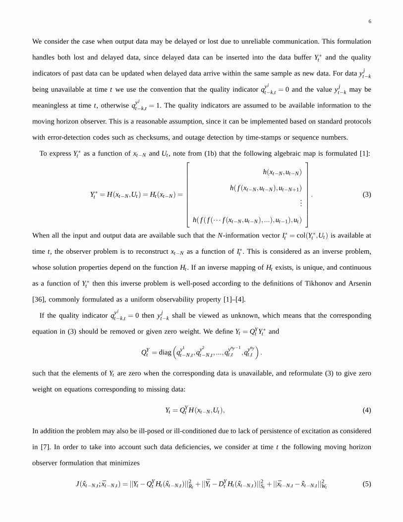
We consider the case when output data may be delayed or lost due to unreliable communication. This formulation

handles both lost and delayed data, since delayed data can beinserted into the data bufferY∗t and the quality

indicators of past data can be updated when delayed data arrive within the same sample as new data. For datay jt−k

being unavailable at timet we use the convention that the quality indicatorqy j

t−k,t = 0 and the valuey jt−k may be

meaningless at timet, otherwiseqy j

t−k,t = 1. The quality indicators are assumed to be available information to the

moving horizon observer. This is a reasonable assumption, since it can be implemented based on standard protocols

with error-detection codes such as checksums, and outage detection by time-stamps or sequence numbers.

To expressY∗t as a function ofxt−N andUt , note from (1b) that the following algebraic map is formulated [1]:

Y∗t = H(xt−N,Ut) = Ht(xt−N) =

h(xt−N,ut−N)

h( f (xt−N,ut−N),ut−N+1)

...

h( f ( f (· · · f (xt−N,ut−N), ...),ut−1),ut)

. (3)

When all the input and output data are available such that theN-information vectorI∗t = col(Y∗t ,Ut) is available at

time t, the observer problem is to reconstructxt−N as a function ofI∗t . This is considered as an inverse problem,

whose solution properties depend on the functionHt . If an inverse mapping ofHt exists, is unique, and continuous

as a function ofY∗t then this inverse problem is well-posed according to the definitions of Tikhonov and Arsenin

[36], commonly formulated as a uniform observability property [1]–[4].

If the quality indicatorqy j

t−k,t = 0 theny jt−k shall be viewed as unknown, which means that the corresponding

equation in (3) should be removed or given zero weight. We defineYt = QYt Y∗

t and

QYt = diag

(

qy1

t−N,t,qy2

t−N,t , ...,qyny−1

t,t ,qyny

t,t

)

.

such that the elements ofYt are zero when the corresponding data is unavailable, and reformulate (3) to give zero

weight on equations corresponding to missing data:

Yt = QYt H(xt−N,Ut), (4)

In addition the problem may also be ill-posed or ill-conditioned due to lack of persistence of excitation as considered

in [7]. In order to take into account such data deficiencies, we consider at timet the following moving horizon

observer formulation that minimizes

J(xt−N,t; xt−N,t) = ||Yt −QYt Ht(xt−N,t)||2Rt

+ ||Yt −DYt Ht(xt−N,t)||2St

+ ||xt−N,t − xt−N,t||2Wt(5)

7

with respect to ˆxt−N,t and subject to

xt−N,t ∈ X (6)

whereRt ,Wt > 0 andSt ≥ 0 are symmetric time-varying weight matrices andDYt = I −QY

t . The weighted Euclidean

norm is defined as||x||P =√

xTPx for vectorsx and some symmetric matrixP> 0. LetJot =minxt−N,t J(xt−N,t; xt−N,t),

and xot−N,t be the associated optimal estimate. It is assumed that the a priori estimator is determined as

xt−N,t = f (xot−N−1,t−1,ut−N−1), (7)

and the a priori estimated output is defined as

Yt = DYt Ht(xt−N,t). (8)

It is remarked that the optimization variable ˆxt−N,t is the state at the beginning of the horizon. Due to knowledgeof

the mappingHt(·), this uniquely defines the state estimates at the entire horizon, including the current state estimate

xt,t that is usually the main target of estimation. It is further remarked that the formulation can be extended with

process noise (as in [2], [4]) or a Kalman-filter corrected predictor for pre-filtering of the a priori estimate (as in

[37], [38]) in order to reduce the estimator’s sensitivity to model errors and disturbances. For simplicity, we leave

out this extension in the present paper.

The cost function (5) consists of three terms. The first term weights the errors between the measured and predicted

outputs on the horizon in a least squares sense. The third term penalizes the difference between the state estimate

at the beginning of the horizon and the one-step-ahead predicted (a priori) state estimate using the open loop model

and the previous optimal state estimate, [4]. As discussed in [7], this term has a regularizing and low-pass filtering

effect on the state estimate at it allows the estimate to degrade to an open loop model estimate when the first term is

not sensitive to some combinations of estimated states. In particular, for detectable systems where a sub-system is

not observable, the third term ensures that the unobservable states are updated according to the stable sub-system’s

open loop model. Moreover, when data are not persistently exciting such that the first term is not sensitive to the

state estimate, the weighting of the third term means that un-excited states are estimated in an open loop fashion.

The second term is less conventional, and introduced in order to put some weight on open loop estimates in cases

when output measurements are not available. This term allows errors in the data to be weighted against errors in

the model. As will be shown in Section III, convergence can beestablished also when this term has zero weight

8

(St = 0) such that this term should be considered optional although it might be useful to improve practical estimator

accuracy in the presence of noise, model errors and missing data.

III. C ONVERGENCE

Before we state the sufficient conditions for convergence ofthe state estimate ˆxt−N,t that minimizes the MHE

cost function, we need to introduce some concepts and definitions. Following [1], the system (1) isN-observable

if there exists aK-function ϕ such that for allx1,x2 ∈ X there exists a feasibleUt ∈ UN+1 such that

ϕ(||x1−x2||2)≤ ||H(x1,Ut)−H(x2,Ut)||2.

The inputUt and the outputY∗t with the measurement qualityQY

t is said to beN-informativefor theN-observable

system (1) at timet if there exists aK-function ϕt that for all x1,x2 ∈ X satisfies

ϕt(||x1−x2||2)≤ ||QYt H(x1,Ut)−QY

t H(x2,Ut)||2.

Systems and data satisfying these properties at all time instants have properties similar to uniformly observable

systems and allow convergence results to be derived. On the other hand, when a system is notN-observable,

it is not possible to reconstruct exactly all the state components from theN-information vector due to lack of

information. However, in some cases one may be able to reconstruct exactly at least some components, based on

theN-information vector, and the remaining components can be reconstructed asymptotically. This corresponds to the

concept of detectability, where we suppose there exists a coordinate transformT :X→D⊆Rnx, d= col(ξ ,z)= T(x)

such that the following dynamics are equivalent to (1),

ξt+1 = F1(ξt ,zt ,ut) (9a)

zt+1 = F2(zt ,ut) (9b)

yt = g(zt ,ut), (9c)

The vectorξt ∈ Rnξ contains un-observable state variables, andzt ∈ Rnz contains observable state variables. Similar

to H(·), the following algebraic map can be formulated [1]:

Y∗t = G(zt−N,Ut) = Gt(zt−N) =

g(zt−N,ut−N)

g(F2(zt−N,ut−N),ut−N+1)

...

g(F2(F2(· · ·F2(zt−N,ut−N), ...),ut−1),ut)

, (10)

9

andYt =QYt G(zt−N,Ut). Before we extend the definition ofN-informativeness toN-detectable systems, we introduce

the concept of incremental input-to-state stability (δ ISS) for the unobservable sub-system (9a) as in [10]. In order

to be able to show exponential convergence of the estimates of the un-observable states, they must, by assumption,

converge exponentially in an open-loop fashion when then observable state estimates converge exponentially.

Although similar assumptions could be made (such as contraction or global exponential stability of the un-perturbed

un-observable sub-system) they would lead to very similar results, and we chose the present formulation in order

to use a similar analysis method as in [9], [10].

A continuous functionV(ξ 1t ,ξ 2

t ,Pξ ) = ||ξ 1t − ξ 2

t ||2Pξwith Pξ = PT

ξ > 0 is called a quadraticδ ISS-Lyapunov

function for the systemξt+1 = F1(ξt ,zt ,ut) if the following holds:

• V(0,0,P) = 0.

• There exist a symmetricQξ > 0 and symmetricΣu > 0,Σz > 0, such that for anyξ 1t ,ξ 2

t and any couple of

input signals(u1t ,u

2t ),(z

1t ,z

2t ),

V(ξ 1t+1,ξ

2t+1,Pξ )−V(ξ 1

t ,ξ2t ,Pξ )≤−V(ξ 1

t ,ξ2t ,Qξ )+V(u1

t ,u2t ,Σu)+V(z1

t ,z2t ,Σz). (11)

The inputUt and the outputY∗t with the measurement qualityQY

t is said to beN-informativefor the N-detectable

system (1) at timet if

(1) there exists a coordinate transformT : X→ D that brings the system in the form (9);

(2) the inputUt and outputY∗t with the measurement qualityQY

t is N-informative for theN-observable sub-system

(9b)-(9c) at timet.

(3) the sub-system (9a) has a quadraticδ ISS-Lyapunov function (11).

As shown by the following result, for arbitrary choices ofSt ≥ 0 andWt > 0 there exists a sufficiently large

Rt > 0 such that the observer estimation erroret−N = xt−N − xot−N,t converges exponentially to zero, under some

conditions.

Theorem 1:Suppose the following assumptions hold

(A1) The functionsf andh are twice differentiable, and the functionsF1,F2 andg are twice differentiable.

(A2) T(x) is continuously differentiable and bounded away from singularity for all x∈X such thatT−1(x) is well

defined.

(A3) The inputUt and outputY∗t with the measurement qualityQY

t are N-informative for all t ≥ 0 for the N-

detectable system (1).

10

(A4) The signalsut , yt andxt are bounded.

(A5) The setX is closed, convex, and controlled invariant,i.e. f(xt ,ut) ∈ X for all xt ∈ X and the controlut ∈ U

for all t ≥ 0.

(A6) For any col(ξ1,z1) ∈ D and col(ξ2,z2) ∈ D, then col(ξ1,z2) ∈ D, col(ξ2,z1) ∈ D.

Then for anySt ≥ 0 andWt > 0 there exists a sufficiently large weight matrixRt > 0 such that for any initial a

priori estimate ¯x0,N ∈ X the observer error converges exponentially to zero.

Proof: Given in the appendix.

We remark that the closed setX is chosen by the user primarily in order to represent physical constraints on the

state estimates, although its choice may be limited due to validity of the model or assumptions that must hold on

this setX. With the choiceX= Rn we get a global exponential convergence result. In other cases, the region of

attraction of the estimate will not be global, but limited bythe setX.

The key assumption is (A3) which requires that the system isN-detectable and the data areN-informative, which

means that there is a sufficient number of exciting measurements are available. This means that the NMHE is

inherently robust to delayed and lost data, provided that the amount of missing data is not too large compared to

the window sizeN. In [21], it was proposed to handle lost data by online adaptation of the window sizeN in order

to guarantee that the window of information isN-informative at each time step. While increasing the windowsize

N will generally improve robustness, it may still not be desirable to do so. The two main reasons are increased

computational complexity of the online nonlinear program,and increased degree of filtering of the estimate that

may be undesired if operating in a non-stationary or highly time-varying environment that requires that the state

estimator adapts quickly to rapidly changing parameters.

In this paper, we take into account that violation of the assumption of N-informative data may be expected, and

the robustness of the NMHE algorithm to such data deficiency can be further enhanced using an adaptive weight

selection algorithm as described in Section IV.

IV. A DAPTIVE WEIGHTING AND FURTHER ROBUSTNESS

This section provides some further regularization mechanisms and tuning guidelines to ensure robustness and

graceful degradation when significant amounts of measurements are delayed or lost. First, we provide a character-

ization of the requirements on the weight matrixRt based on Theorem 1 for the case when the assumptions are

fulfilled.

11

Proposition 1: Define the following matrixes

Γt−1 = Γt−1(xt−N−1, xot−N−1,t−1) =

∫ 1

0

∂∂x

T((1−s)xt−N−1+sxot−N−1,t−1)ds,

Λt = Γ−1t−1

TΘTt (∆

Tt St∆t +Wt)ΘtΓ−1

t−1,

Ψt = Ψt(xt−N, xot−N,t) = QY

t

∫ 1

0

∂∂x

H((1−s)xt−N+sxot−N,t,Ut)ds.

where∆t and Θt are defined in Lemma 2 in the Appendix. For a suitable scalarα > 0, matrix Ξ = ΞT > 0, and

matrix P2 = PT2 > 0 for all t ≥ 0, if the weight matrixRt is chosen such that the following matrix inequalities holds,

whereη = [0nz×nξ , Inz],

ηΓ−1t

TΨTt RtΨtΓ−1

t ηT ≥ P2, (12a)

αQξ 0

0 P2−αΣz

> Ξ+Λt , (12b)

then the observer error is exponentially stable.

Proof: See Appendix.

Fulfillment of eq. (12a) at all time instantst requires thatΨt has full rank, which is guaranteed by data being

N-informative. Eq. (12a) ensures that the chosen Lyapunov function decreases at each time instant. This is a

sufficient condition that may not be necessary, and it may be sufficient that the Lyapunov function ”decreases in

average” as commonly exploited when using the concept of persistence of excitation. Intuitively, it is therefore

reasonable to believe that some stability and convergence properties can still be achieve if this assumption is mildly

violated, assuming that there are ”enough measurements on average”. Due to the second and third terms in the cost

function, the estimator functionality degrades to an open loop observer in such cases, with selectivity such that the

available measurements are still fully utilized in situations with partial measurements being available (like one of

two outputs available). As discussed in [7], these regularization mechanisms may be sufficient in cases when the

system is open loop asymptotically stable. However, when the system is marginally stable (e.g. by joint identification

of parametersθ with a state augmentation of the model withθ = 0), or unstable, the open loop integration of the

model in the estimator may lead to drifting estimates. As described in [39]–[42], the use of directional updating

based on a decomposition of the information matrix can be used to prevent updating of combinations of state

variables for which no information exists in the data. Effectively, this prevents drifting estimates due to noise

and model errors that would otherwise be the dominant driving force of the estimate updates. Following [7] we

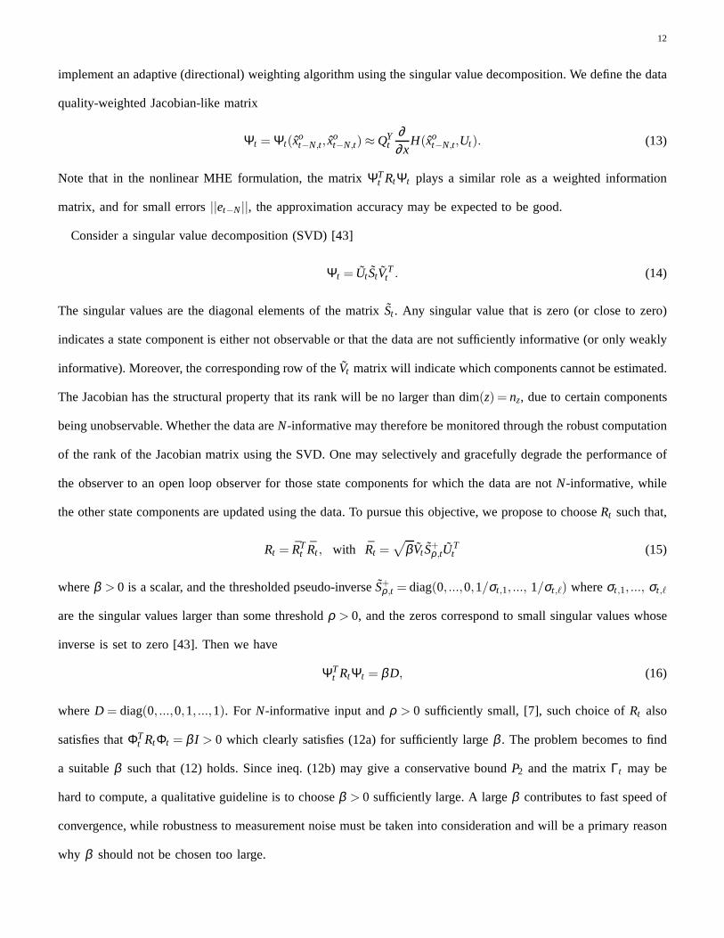
12

implement an adaptive (directional) weighting algorithm using the singular value decomposition. We define the data

quality-weighted Jacobian-like matrix

Ψt = Ψt(xot−N,t, x

ot−N,t)≈ QY

t∂∂x

H(xot−N,t,Ut). (13)

Note that in the nonlinear MHE formulation, the matrixΨTt RtΨt plays a similar role as a weighted information

matrix, and for small errors||et−N||, the approximation accuracy may be expected to be good.

Consider a singular value decomposition (SVD) [43]

Ψt = UtStVT

t . (14)

The singular values are the diagonal elements of the matrixSt . Any singular value that is zero (or close to zero)

indicates a state component is either not observable or thatthe data are not sufficiently informative (or only weakly

informative). Moreover, the corresponding row of theVt matrix will indicate which components cannot be estimated.

The Jacobian has the structural property that its rank will be no larger than dim(z) = nz, due to certain components

being unobservable. Whether the data areN-informative may therefore be monitored through the robustcomputation

of the rank of the Jacobian matrix using the SVD. One may selectively and gracefully degrade the performance of

the observer to an open loop observer for those state components for which the data are notN-informative, while

the other state components are updated using the data. To pursue this objective, we propose to chooseRt such that,

Rt = RTt Rt , with Rt =

√

βVt S+ρ ,tU

Tt (15)

whereβ > 0 is a scalar, and the thresholded pseudo-inverseS+ρ ,t = diag(0, ...,0,1/σt,1, ..., 1/σt,`) whereσt,1, ..., σt,`

are the singular values larger than some thresholdρ > 0, and the zeros correspond to small singular values whose

inverse is set to zero [43]. Then we have

ΨTt RtΨt = βD, (16)

whereD = diag(0, ...,0,1, ...,1). For N-informative input andρ > 0 sufficiently small, [7], such choice ofRt also

satisfies thatΦTt RtΦt = β I > 0 which clearly satisfies (12a) for sufficiently largeβ . The problem becomes to find

a suitableβ such that (12) holds. Since ineq. (12b) may give a conservative boundP2 and the matrixΓt may be

hard to compute, a qualitative guideline is to chooseβ > 0 sufficiently large. A largeβ contributes to fast speed of

convergence, while robustness to measurement noise must betaken into consideration and will be a primary reason

why β should not be chosen too large.

13

Scaling of the model equations and variables is instrumental for the approach since the thresholded singular value

decomposition is used to determine directions in the parameter space that should be updated based on data, and

those that are not to be updated due to lack of information. Inorder to allow a direct comparison of the (scalar)

singular values, all variables need to be scaled appropriately. Numerical robustness and simplification of the tuning

are other good reasons for scaling. Determining the scalingfactors is usually done in two steps. First, rough scaling

in order to account for different physical units, e.g. scaleall to a range 0-100. Second, some fine tuning of the

scaling in order to maximize the performance of the observer. This usually requires an iterative procedure with

some trial and error having in mind the importance of the individual variables in a given application.

For inputs that are notN-informative, the parameterρ > 0 may be tuned in order to enhance robustness of the

algorithm such thatRt gives zero weight on state combinations for which there is insufficient information. The

qualitative guideline is that increasedρ will require a higher degree of information in order to update estimates and

thereby improve robustness to noise, missing data and modeluncertainties at the cost of convergence speed. The

choice ofρ may require extensive simulation and experimental testingsince the primary objective of the thresholded

SVD is to avoid undesired parameter estimator drift due to model errors under conditions characterized by lack

of excitation or too little available data. It may also require re-tuning of the weights inWt and some re-scaling of

variables in order to tune the responses of the individual parameter estimates.

The 2nd term in the NMHE criterion, weighted withSt , is introduced to allow simulated output data to be used

as a substitute when real measurements are not available. The elements ofSt are tuning parameters that should

increase with the confidence in the model, increase with measurement noise levels, but should usually be less than

Rt since real measurements should be trusted more than simulated measurements.

Clearly, the choice of window sizeN is important for the performance of the algorithm. There areseveral effects

involved. First, an increased window sizeN will lead to a high degree of low-pass filtering in the MHE. This has

the benefits that effects of uncertainties such as noise, missing data and model errors are reduced, while the main

drawbacks are reduced speed of convergence and increased computational load. Moreover, for a given application

there is a minimumN ≤ n that is necessary in order to achieveN-observability of the system. It should be remarked

that increasingN is not the only option for increasing the degree of low-pass filtering within the MHE, as increasing

the weights inWt will also have this effect.

We mention that the diagnostic information resulting from the singular value decomposition could potentially

be used to prioritize re-transmission requests for critical data while less important data need not be requested to

14

be re-transmitted. This contributes to the overall objective of greedy use of communication capacity in order to

improve overall communication performance in terms of latency, power consumption, and data integrity.

V. SUMMARY OF ALGORITHM

In summary, the estimation algorithm consists of the following steps

1) Initialization: N, Wt , St , x0,N, X, β , ρ

2) Acquire new data, and stack into the moving window vectorsUt andY∗t and associated quality indicatorsQY

t

andDYt = I −QY

t ..

3) GenerateYt according to (4) andYt according to (8).

4) Compute the approximation ofΨt according to (13) using numerical finite difference approximations or

analytical expressions.

5) Compute the SVD ofΨt , cf. (14) and [43].

6) ComputeRt according to (15).

7) Solve the nonlinear programming problem with objective function (5) and constraints (6) using a numerical

solvers (such as NPSOL that was used in the examples) for the updated state estimate ˆxt−N,t .

8) Update the a priori estimate according to (7), and return to step 2 for the next update.

VI. EXAMPLES

A simulation example is first used to illustrate the main ideas, while the performance of the approach is evaluated

using experimental data from an offshore oil well drilling operation in the second example. In the examples we

use the NPSOL sequential quadratic programming algorithm to solve the nonlinear MHE problems. Matlab is used

for simulation and other computations, with the TOMLAB interface to NPSOL.

A. Example 1 - mixed state and parameter estimation

Consider the following system

x1 =−4x1+x2 (17a)

x2 =−x2+x3u (17b)

x3 = 0 (17c)

y= x2+v. (17d)

15

It is clear thatx1 is not observable, but corresponds to aδ ISS system, whilex2 and x3 are observable state

variables. It is also clear that our ability to exactly compute x3 from measured input and output data will depend

on the excitationu, while x2 is uniformly observable. One may think ofx3 as a parameter representing an unknown

gain on the input, where the third state equation is an augmentation for the purpose of estimating this parameter.

The same observability and detectability properties hold for the discretized system with sampling intervalt f = 0.1s.

It is easy to see that the sub-system (17a) has a quadraticδ ISS-Lyapunov function.

In the example, the inputu is discrete-time white noise, which is highly exciting. Independent uniformly

distributed measurement noisev ∈ [−0.05,0.05] is added to the output. Different scenarios are generated by

simulating different percentages of lost output measurements. A window sizeN = 8 was chosen. This window

is larger than the theoretical minimum, which was found to improve the robust performance of the method. The

criterion weight parameters are set toSt = 0.1I andWt = 0.7I , and use the adaptive weighting law (15) to define

Rt usingβ = 10. This tuning was made as a trade-off between fast responseand sensitivity to noise. The threshold

δ = 0.01 was tuned to avoid drifting estimates during periods withinsufficient measurements.

We evaluate the NMHE performance using the root mean square error

RMSE =

(

1M

M

∑t=0

||et ||2)1/2

,

whereet is the estimation error at timet, andM = 100 is the length of the simulation run. The simulation results

with different measurement loss probabilities, and the average ofRMSEof state estimates, are shown in Table I for

20 different initial states. Table II shows the results obtained by the method in [19], where the Extended Kalman

Filter (EKF) is implemented with mechanisms to handle intermittent observations. For the EKF, it is assumed that

the disturbance standard deviation is 0.0167 and the same initial estimates were used in the EKF and NMHE.

From Table I and Table II, it can be concluded that the accuracy of the proposed NMHE method is better than the

implemented EKF.

Figure 1 shows the estimates of these two methods with the same initial state estimate when the probability of

missing data is 80%. From Figure 1, it can be observed thatx3 estimated by the EKF is updated only when new

measurements become available, which leads to a somewhat slow response. On the other hand,x3 estimated by

the proposed NMHE is updated at each time step due to the window of data, which results in improved accuracy

compared to the implemented EKF. It takes on average around 50 ms to compute the state estimate with the NMHE

method at each step, while the computation time of the EKF is around 5 ms. Although these computations are

16

made in Matlab on a standard PC without any attempt to optimize the implementation for computational efficiency,

we believe their ratio is a fairly valid indicator of their computational performance ratio.

The results shows that performance degrades gracefully, with fairly small reduction in estimation accuracy up to

about 30 % loss probability. Even at 80 % loss the estimator gives robust estimates with performance degradation

of a factor less than 5.

Loss Probs(%) 0 2 5 10 20 30 50 70 80

RMSE of x1 0.0605 0.0605 0.0604 0.0604 0.0603 0.0603 0.0601 0.0618 0.0715

RMSE of x2 0.0097 0.0098 0.0118 0.0155 0.0216 0.0285 0.0326 0.0364 0.0375

RMSE of x3 0.0149 0.0153 0.0158 0.0176 0.0203 0.0238 0.0517 0.0653 0.0746

TABLE I

EXAMPLE 1: THE ESTIMATION ERRORS OF THE PROPOSEDMHE.

Loss Probs(%) 0 2 5 10 20 30 50 70 80

RMSE of x1 0.0702 0.0704 0.0704 0.0705 0.0701 0.0701 0.0709 0.0716 0.0721

RMSE of x2 0.0226 0.0247 0.0284 0.0359 0.0416 0.0459 0.0511 0.0571 0.0588

RMSE of x3 0.0728 0.0863 0.1236 0.1316 0.1320 0.1474 0.1645 0.2026 0.2080

TABLE II

EXAMPLE 1: THE ESTIMATION ERRORS OF THEEKF.

B. Example 2 - Estimation of Bottom Hole Pressure during Oil Well Drilling

In this example, we here implement the proposed approach to estimate the bottom hole pressure (BHP) during

a Managed Pressure Drilling (MPD) operation. MPD is a drilling process used to precisely control an annular

pressure profile throughout the well bore, cf. Figure 2. The drilling fluid (commonly called mud) is pumped down

the rotating drillpipe. At the drill bit at the bottom of the hole the fluid is allowed to flow through the drill bit

as it rotates to make the hole, and circulate back to the top side through the annulus. The purpose of this flow is

twofold. First, it removes cuttings from the drilling at thebottom hole, and second, it provides a pressure in the

well that acts as a barrier against uncontrolled inflow of hydrocarbons that might occur if an oil or gas reservoir is

penetrated. The pressure should be controlled accurately within the range between the pore pressure of the reservoir

and the fracture pressure, beyond which the drilling fluid may cause damage to the well bore, using the choke or

17

10 20 30 40 50 60 70 80 90 100−1.5

−1

−0.5

0

0.5

t

x1

x1 with 80% data loss probability by MHE

x1 with 80% data loss probability by Kalman Filter

x1 by measurements

10 20 30 40 50 60 70 80 90 100−6

−4

−2

0

2

t

x2



x2 by measurements

10 20 30 40 50 60 70 80 90 100

1.6

1.8

2

2.2

t

x3



x3 by measurements

time with new data

Fig. 1. Example 1: Estimates with loss probability being 80%.

18

back-pressure pump. The circulation of the drilling fluid also involves some top-side processing in order to remove

foreign elements from the fluid before it is circulated.

To model the MPD drilling system for use in the estimator, we use a simplified model developed in [44]. The

parameters used in the example are given in Table III.

Fig. 2. A simplified drawing of the MPD drilling system.

The MPD system can be described as

pc =βa

Va(qb−qc+qback+Va), (18a)

pp =βd

Vd(qpump−qb), (18b)

qb =1M(pp− pc−λ1q2

pump−λ2(qc−qback)2+(ρd−ρa)gh), (18c)

with the parametersM = Ma+Md with Ma = ρa∫ `a

o1

Aa(x)dx and Md = ρd

∫ `do

1Ad(x)

dx. The pressure of the bottom

hole, pbit (also called bottom hole pressure - BHP), depends on the choke pressure, pump pressure, frictional loss

pressure and hydrostatic pressure, which is given as

pbit =Ma

Mpp+

Md

Mpc+

Md

Mλ2(qc−qback)

2− Ma

Mλ1q2

pump+(Md

Mρa+

Ma

Mρd)gh. (19)

In this example, it is assumed that the parametersλ1,λ2 are unknown. With this parametrization one has to expect

19

Parameters Description Unit

Va Annulus volume m3

Vd Drill string volume m3

βa Bulk modulus of fluid in annulus bar

βd Bulk modulus of fluid in drill string bar

pc Choke pressure bar

pp Pump pressure bar

qb Flow rate of the bit m3/s

qc Flow rate of the choke m3/s

qback Flow rate of the backpressure pump m3/s

qpump Flow rate of the pump m3/s

λ1 Friction parameter of drill string bars2/m6

λ2 Friction parameter of annulus bars2/m6

ρa Density mud in annulus kg/m3

ρd Density mud in drill string kg/m3

g Acceleration of gravity m/s2

h Vertical depth of the bit m

`a Length of annulus m

`d Length of drill string m

Aa Cross sectional area of annulus m2

Ad Cross sectional area of drill string m2

pbit Bottom hole pressure bar

TABLE III

MODEL VARIABLES.

that the model is over-parameterized such that the persistence of excitation condition (and uniform observability)

will not hold. This challenging parametrization is chosen in order to illustrate the power of the proposed method,

and in particular that the algorithm will accurately detectthe information content of the available data at any time

and adapt the weights accordingly when usingRt defined by (15). Therefore, the proposed NMHE algorithm is

applied to the combined state and parameter estimation problem by considering the parametersλ1,λ2 as augmented

states,λ1 = 0, andλ2 = 0. The constraints on the states and estimations are given as

pc ≥ 0, pp ≥ 0, qb ≥ 0, λ1 ≥ 0, λ2 ≥ 0, pbit ≥ 0. (20)

Some parameters such asqpump,qc,qback,ρa,ρd,h, `a, `d, pc andpp can be measured by sensors while drilling. These

20

are available att f = 1 s sampling rate from the top-side instrumentation and drilling mud logging system. Then

the corresponding states, inputs and outputs and time-varying disturbances are given as

x=

pc

pp

qb

λ1

λ2

, u=

h

ρa

ρd

qpump

qc

qback

, y=

pc

pp

, w= Va, (21)

whereVa = Ah is a known input.

The available data consists of an experimental time series from an MPD drilling operation in the North Sea.

The input signals are shown in Figure 3. Some of the measurements are noisy and also contain outright errors in

some places. There are several uncertainties in drilling operation due to missing and inaccurate configuration data

(inaccurate well profile plan compared with that actual achieved). Normally 5 bar difference between true BHP and

estimated BHP is to be expected in many cases.

The window size is chosen asN = 10. We choose the tuning parameters of the cost function asSt = 0.01I and

Wt = 0.3I , and utilize the SVD-based adaptive weighting law with tuning parametersβ = 0.1 andρ = 0.001 to

defineRt . The state variables are scaled with factors 0.1 for pc, 0.1 for pp, 1 for qb, and 0.001 for bothλ1 and

λ2. These tuning parameters were found after some trial and error in order to achieve a satisfactory combination

of fast estimation and high robustness to uncertainties such as noise and data losses. Our experience is that the

performance is not very sensitive to the choice of tuning parameters.

In the base case all data points are available, while different data sets with different loss probabilities were

generated by randomly and independently picking out a certain percentage of the data points. Table IV shows the

different measurement loss probabilities and RMSE betweenmeasurements and the estimations duringttotal = 1650s.

Table V shows the accuracy of the implemented EKF, [19], indicating that better accuracy in estimating the BHP

is achieved with the NMHE method. The average computation time is around 400 ms at each step for the NMHE

method, while it takes 30 ms for EKF. Although these computations are made in Matlab on a standard PC without any

attempt to optimize the implementation for computational efficiency, we believe their ratio is a fairly valid indicator

of their computational performance ratio. Comparison of the accuracy between estimates and experimental data

with data loss probabilities in the range of 0-70 % are shown in Figures 4 - 8.

21

0 200 400 600 800 1000 1200 1400 16001646

1648

1650

t

h

0 200 400 600 800 1000 1200 1400 16000.015

0.016

0.017

t

ρa

0 200 400 600 800 1000 1200 1400 16000.015

0.016

0.017

t

ρd

0 200 400 600 800 1000 1200 1400 16000

0.02

0.04

t

qp

um

p

0 200 400 600 800 1000 1200 1400 16000

0.02

0.04

t

qc

0 200 400 600 800 1000 1200 1400 1600−1

0

1

t

qb

ack

Fig. 3. Example 2: Input measurements.

22

0 200 400 600 800 1000 1200 1400 16000

20

40

t

pc

pc with 0% data loss probability

pc by measurements

0 200 400 600 800 1000 1200 1400 16000

100

200

t

pp

pp with 0% data loss probability

pp by measurements

0 200 400 600 800 1000 1200 1400 1600260

280

300

t

BH

P

BHP with 0% data loss probabilityBHP by memories

0 200 400 600 800 1000 1200 1400 16000

0.05

t

qb

0 200 400 600 800 1000 1200 1400 16001

1.5

2x 10

5

t

λ1

0 200 400 600 800 1000 1200 1400 16000

2

4x 10

4

t

λ2

Fig. 4. Example 2: Loss probability being 0%.

23

0 200 400 600 800 1000 1200 1400 16000

20

40

t

pc


pc by measurements

0 200 400 600 800 1000 1200 1400 16000

100

200

t

pp


pp by measurements

0 200 400 600 800 1000 1200 1400 1600260

280

300

t

BH

P


0 200 400 600 800 1000 1200 1400 16000

0.05

t

qb

0 200 400 600 800 1000 1200 1400 16001

1.5

2x 10

5

t

λ1

0 200 400 600 800 1000 1200 1400 16000

2

4x 10

4

t

λ2


24

0 200 400 600 800 1000 1200 1400 16000

20

40

t

pc

0 200 400 600 800 1000 1200 1400 16000

100

200

t

pp

0 200 400 600 800 1000 1200 1400 1600260

280

300

t

BH

P

0 200 400 600 800 1000 1200 1400 16000

0.05

t

qb

0 200 400 600 800 1000 1200 1400 16001

2

3x 10

5

t

λ1

0 200 400 600 800 1000 1200 1400 16000

1

2x 10

5

t

λ2


pp by measurements



pc by measurements


25

0 200 400 600 800 1000 1200 1400 16000

20

40

t

pc

0 200 400 600 800 1000 1200 1400 16000

100

200

t

pp

0 200 400 600 800 1000 1200 1400 1600260

280

300

t

BH

P

0 200 400 600 800 1000 1200 1400 16000

0.05

t

qb

0 200 400 600 800 1000 1200 1400 16001

2

3x 10

5

t

λ1

0 200 400 600 800 1000 1200 1400 16000

1

2x 10

5

t

λ2


pc by measurements


pp by measurements



26

0 200 400 600 800 1000 1200 1400 16000

20

40

t

pc


pc by measurements

0 200 400 600 800 1000 1200 1400 16000

100

200

t

pp


pp by measurements

0 200 400 600 800 1000 1200 1400 1600260

280

300

t

BH

P


0 200 400 600 800 1000 1200 1400 16000

0.05

t

qb

0 200 400 600 800 1000 1200 1400 16001

2

3x 10

5

t

λ1

0 200 400 600 800 1000 1200 1400 16000

1

2x 10

5

t

λ2


27

Loss Probs(%) 0 2 10 30 50 70

RSME (bar) ofpc 0.1274 0.1297 0.1285 0.3870 0.3858 0.8559

RSME (bar) ofpp 0.2071 0.2179 0.2192 0.3386 0.4149 0.9396

RSME (bar) ofpbit(BHP) 0.9905 0.9923 1.0092 1.1889 1.4067 1.4824

TABLE IV

EXAMPLE 2: THE ESTIMATION ERROR OF THE PROPOSEDMHE.

Loss Probs(%) 0 2 10 30 50 70

RSME (bar) ofpc 0.0847 0.0894 0.1136 0.1748 0.3471 0.8285

RSME (bar) ofpp 0.3592 0.3647 0.4082 0.4829 0.7403 1.3260

RSME (bar) ofpbit(BHP) 1.1963 1.2015 1.3137 1.4689 1.9167 2.1025

TABLE V

EXAMPLE 2: THE ESTIMATION ERROR OF THEEKF.

VII. C ONCLUSIONS

The use of nonlinear moving horizon estimation are studied for applications where output data may be lost or

delayed due to unreliable digital communication. The contribution of the paper are nonlinear MHE formulations and

weight selection methods that ensures robustness modifications using regularization. The regularizing mechanisms

are stabilizing terms in the cost function that ensures graceful degradation to an open loop observer, and a SVD-

based weight selection method that avoids drift of estimates when data are not informative and the dynamic model

of the plant does not have strong enough internal open loop stability. Simulation and experimental results from

an oil well drilling application shows that the performanceof the nonlinear MHE degrades gracefully even when

output measurements are lost with a probability above 50 %.

APPENDIX

Lemma 1:Define the matrix

Ωt =Ωt(zt−N, zot−N,t) = QY

t

∫ 1

0

∂∂z

G((1−s)zt−N+szot−N,t,Ut)ds.

ThenΩTt RtΩt > 0 for all t and

Jot ≥ ||zt−N − zo

t−N,t||2ΩTt RtΩt

. (22)

Proof: Using the fact that the system (1a)-(1b) can be transformed using T, there existdt−N = T(xt−N),

dot−N,t = T(xo

t−N,t) and dt−N,t = T(xt−N,t) such that in the new coordinates, the system is in the form of (9a)-(9c).

28

Note that the first term in the right-hand side of expression (5) in the new coordinations can be rewritten as

||Yt −QYt H(xo

t−N,t,Ut)||2Rt= ||QY

t G(zt−N,Ut)−QYt G(zo

t−N,t,Ut)||2Rt.

From Proposition 2.4.7 in [45],

QYt G(zt−N,Ut)−QY

t G(zot−N,t,Ut) = Ωt(zt−N− zo

t−N,t).

and we have

||QYt G(zt−N,Ut)−QY

t G(zot−N,t,Ut)||2Rt

= ||zt−N − zot−N,t||2ΩT

t RtΩt.

Taking zero as the lower bound on the rest terms of (5), we get (22). Since the data areN-informative, the matrix

Ωt has full rank andΩTt RtΩt > 0 for all t.

Lemma 2:Define the matrices

∆t = ∆t(xt−N,t,xt−N) = DYt

∫ 1

0

∂∂x

H((1−s)xt−N,t +sxt−N,Ut)ds,

Θt = Θt(xot−N−1,t−1,xt−N−1) =

∫ 1

0

∂∂x

f ((1−s)xot−N−1,t−1+sxt−N−1,ut−N−1)ds.

Then

Jot ≤ ||xt−N−1− xo

t−N−1,t−1||2ΘTt (∆T

t St∆t+Wt)Θt. (23)

Proof: We know thatxt−N ∈ X is a feasible solution at timet. From the optimality of ˆxot−N,t, we haveJo

t ≤

J(xt−N; xt−N,t). Then considering the cost functionJ(xt−N; xt−N,t), we have||Yt −QYt H(xt−N,Ut)||2Rt

= 0. Like the

proof of Lemma 1, the second term in the right-hand side of expression (5) can be rewritten as

||Yt −DYt H(xt−N,Ut)||2St

= ||DYt H(xt−N,t,Ut)−DY

t H(xt−N,Ut)||2St= ||xt−N,t −xt−N||∆T

t St∆t.

Similarly,

xt−N,t −xt−N = Θt(xot−N−1,t−1−xt−N−1).

Then, the terms of the right-hand side of expression (5) can be written as (23).

Proof of Theorem 1:

Consider a Lyapunov functionV(st)= ||s1t ||2P1

+ ||s2t ||2P2

, wherest = col(s1t ,s

2t ), P1=αPξ ,α >0 andP2=PT

2 > 0 for

all t ≥ 0. Then it is easy to show thatV(st)> 0 andV(0)= 0 for all t ≥ 0. Lets1t = ξt−N− ξ o

t−N,t , s2t = zt−N− zo

t−N,t . In

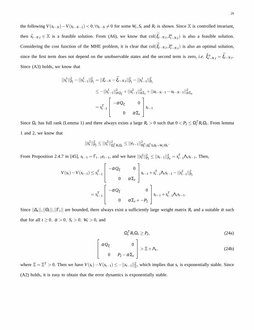
29

the followingV(st−N)−V(st−N−1)< 0,∀st−N 6= 0 for someWt ,St andRt is shown. SinceX is controlled invariant,

then xt−N,t ∈ X is a feasible solution. From (A6), we know that col(ξt−N,t, zot−N,t) is also a feasible solution.

Considering the cost function of the MHE problem, it is clearthat col(ξt−N,t, zot−N,t) is also an optimal solution,

since the first term does not depend on the unobservable states and the second term is zero,i.e. ξ ot−N,t = ξt−N,t .

Since (A3) holds, we know that

||s1t ||2P1

−||s1t−1||2P1

= ||ξt−N − ξt−N,t||2P1−||s1

t−1||2P1

≤−||s1t−1||2αQξ

+ ||s2t−1||2αΣz

+ ||ut−N−1−ut−N−1||2αΣu

= sTt−1

−αQξ 0

0 αΣz

st−1

SinceΩt has full rank (Lemma 1) and there always exists a largeRt > 0 such that 0< P2 ≤ ΩTt RtΩt . From lemma

1 and 2, we know that

||s2t ||2P2

≤ ||s2t ||2ΩT

t RtΩt≤ ||et−1||2ΘT

t (∆Tt St∆t+Wt)Θt

.

From Proposition 2.4.7 in [45],st−1 = Γt−1et−1, and we have||s2t ||2P2

≤ ||st−1||2Λt= sT

t−1Λtst−1. Then,

V(st)−V(st−1)≤ sTt−1

−αQξ 0

0 αΣz

st−1+sT

t−1Λtst−1−||s2t−1||2P2

= sTt−1

−αQξ 0

0 αΣz+−P2

st−1+sT

t−1Λtst−1.

Since||∆t ||, ||Θt ||, ||Γt || are bounded, there always exist a sufficiently large weight matrix Rt and a suitableα such

that for all t ≥ 0, α > 0, St > 0, Wt > 0, and

ΩTt RtΩt ≥ P2, (24a)

αQξ 0

0 P2−αΣz

> Ξ+Λt , (24b)

whereΞ = ΞT > 0. Then we haveV(st)−V(st−1)≤−||st−1||2Ξ, which implies thatst is exponentially stable. Since

(A2) holds, it is easy to obtain that the error dynamics is exponentially stable.

30

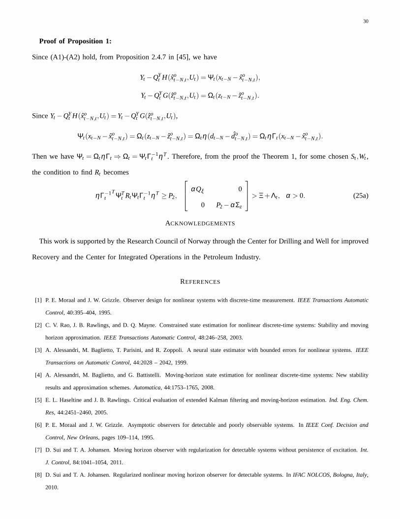
Proof of Proposition 1:

Since (A1)-(A2) hold, from Proposition 2.4.7 in [45], we have

Yt −QYt H(xo

t−N,t,Ut) = Ψt(xt−N− xot−N,t),

Yt −QYt G(zo

t−N,t,Ut) = Ωt(zt−N− zot−N,t).

SinceYt −QYt H(xo

t−N,t,Ut) =Yt −QYt G(zo

t−N,t,Ut),

Ψt(xt−N− xot−N,t) = Ωt(zt−N− zo

t−N,t) = Ωtη(dt−N− dot−N,t) = ΩtηΓt(xt−N− xo

t−N,t).

Then we haveΨt = ΩtηΓt ⇒ Ωt = ΨtΓ−1t ηT . Therefore, from the proof the Theorem 1, for some chosenSt ,Wt ,

the condition to findRt becomes

ηΓ−1t

TΨTt RtΨtΓ−1

t ηT ≥ P2,

αQξ 0

0 P2−αΣz

> Ξ+Λt, α > 0. (25a)

ACKNOWLEDGEMENTS

This work is supported by the Research Council of Norway through the Center for Drilling and Well for improved

Recovery and the Center for Integrated Operations in the Petroleum Industry.

REFERENCES

[1] P. E. Moraal and J. W. Grizzle. Observer design for nonlinear systems with discrete-time measurement.IEEE Transactions Automatic

Control, 40:395–404, 1995.

[2] C. V. Rao, J. B. Rawlings, and D. Q. Mayne. Constrained state estimation for nonlinear discrete-time systems: Stability and moving

horizon approximation.IEEE Transactions Automatic Control, 48:246–258, 2003.

[3] A. Alessandri, M. Baglietto, T. Parisini, and R. Zoppoli. A neural state estimator with bounded errors for nonlinearsystems.IEEE

Transactions on Automatic Control, 44:2028 – 2042, 1999.

[4] A. Alessandri, M. Baglietto, and G. Battistelli. Moving-horizon state estimation for nonlinear discrete-time systems: New stability

results and approximation schemes.Automatica, 44:1753–1765, 2008.

[5] E. L. Haseltine and J. B. Rawlings. Critical evaluation of extended Kalman filtering and moving-horizon estimation.Ind. Eng. Chem.

Res, 44:2451–2460, 2005.

[6] P. E. Moraal and J. W. Grizzle. Asymptotic observers for detectable and poorly observable systems. InIEEE Conf. Decision and

Control, New Orleans, pages 109–114, 1995.

[7] D. Sui and T. A. Johansen. Moving horizon observer with regularization for detectable systems without persistence of excitation. Int.

J. Control, 84:1041–1054, 2011.

[8] D. Sui and T. A. Johansen. Regularized nonlinear moving horizon observer for detectable systems. InIFAC NOLCOS, Bologna, Italy,

2010.

31

[9] D. Sui and T. A. Johansen. Exponential stability of regularized moving horizon observer forn-detectable nonlinear systems. InProc.

9th IEEE International Conference on Control and Automation (ICCA11), Santiago, Chile, pages 806–811, 2011.

[10] D. Sui and T. A. Johansen. On the exponential stability of moving horizon observer for globally N-detectable nonlinear systems.Asian

J. Control, 12, 2012.

[11] D. E. Quevedo, A. Ahlen, and K. H. Johansson. Stabilityof state estimation over sensor networks with markovian fading channels. In

Proc. IFAC World Congress, Milano, 2011.

[12] H. Foss. Innovations in integrated control systems. InProc. MTS Dynamic Positioning Conference, Houston, 2006.

[13] A. Caiti, V. Calabro, and A. Munafo. Auv team cooperation: emerging behaviours and networking modalities. InIFAC Conference on

Manoeuvring and Control of Marine Craft, Arenzano, Italy, 2012.

[14] N. Nahi. Optimal recursive estimation with uncertain observation.IEEE Trans. Information Theory, 15:457–462, 1969.

[15] M. Hadidi and S. Schwartz. Linear recursive state estimators under uncertainty observations.IEEE Trans. Information Theory, 24:944–

948, 1979.

[16] A. S. Matveev and A. V. Savkin. The problem of state estimation via asynchronous communication channels with irregular transmission

times. IEEE Trans. Automatic Control, 48:670–676, 2003.

[17] B. Sinopoli, L. Schenato, M. Franceschetti, K. Poolla,M. I. Jordan, and S. S. Sastry. Kalman filtering with intermittent observations.

IEEE Trans. Automatic Control, 49:1453–1464, 2004.

[18] S. C. Smith and P. Seiler. Estimation with lossy measurements: Jump estimators for jump systems.IEEE Trans. Automatic Control,

48:2163–2170, 2003.

[19] S. Kluge, K. Reif, and M. Brokate. Stochastic stabilityof the extended kalman filter with intermittent observations. IEEE Trans.

Automatic Control, 55:514 – 518, 2010.

[20] P. Philipp and B. Lohmann. Moving horizon estimation for nonlinear networked control systems with unsynchronizedtimescales. In

Preprints 18th IFAC World Congress, Milano, pages 12457–12464, 2011.

[21] Z. Jin, C.-K. Ko, and R. M. Murray. Estimation for nonlinear dynamics systems over packet-dropping networks. InProc. American

Control Conference, New York, NY, pages 5037–5042, 2007.

[22] J. do Val and E. Costa. Stability of receding horizon Kalman filter in state estimation of linear time-varying systems. In Proceedings

of the 39th IEEE Conference on Decision and Control, 2000.

[23] B. K. Kwon, S. Han, H. Lee, and W. H. Kwon. A receding horizon Kalman filter with the estimated initial state on the horizon. In

International Conference on Control, Automation and Systems, pages 1686 –1690, 2007.

[24] M. R. Akhondi, A. Talevski, S. Carlsen, and S. Petersen.Applications of wireless sensor networks in the oil, gas andresource industries.

In IEEE Int. Conf. Advanced Information Networking and Applications, pages 941–948, 2010.

[25] P. Tubel, C. Bergeron, and S. Bell. Mud pulse telemetry system for down hole meaurement-while-drilling. InProc. IEEE Instrumentation

and Measurement Technology Conf, pages 219–223, 1992.

[26] Z. Jianhui, W. Liyan, L. Fan, and L. Yanlei. An effectiveapproach for the noise removal of mud pulse telemetry system. In The 8th

Int. Conf. Eletronic Measurement and Instrumentation, pages 971–974, 2007.

[27] R. W. Tennent and W. J. Fitzgerald. Passband complex fractionally-spaced equalization of MSK signals over the mud pulse telemetry

channel. InProf. IEEE 1st Workshop on Signal Processing Advances in Wireless Communication, 1997.

32

[28] H. Wolter et al. The first offshore use of an ultrahigh-speed drillstring telemtry network involving a full LWD logging suite and

rotary-steerable drilling system. InProc. SPE Annual Tech. Conf. and Exhibition, Anaheim, page SPE 110939, 2007.

[29] S. Hovda, H. Wolter, G.-O. Kaasa, and T. S. Ølberg. Potential of ultra high-speed drill string telemetry in future improvements of the

drilling process control. InProc. IADC/SPE Asia Pacific Drilling Tech. Conf. Exhib., Jakarta, page IADC/SPE 115196, 2008.

[30] K. Xuanchao and C. Guojian. The research of informationand power transmission property for intelligent drillstring. In Proc. 2nd

Int. Conf. Information Technology and Computer Science, Kiev, pages 174–177, 2010.

[31] F. Iversen et al. Offshore drilling field test of a new system for model integrated closed-loop drilling control. InProc. IADC/SPE

Drilling Conference, Orlando, pages 518–520, 2009.

[32] J. Thorogood, W. Aldred, F. Florence, and F. Iversen. Drilling automation: Technologies, terminology and parallels with other industries.

In Proc. SPE/IADC Drilling Conf. Exhib., Amsterdam, page SPE/IADC 119884, 2009.

[33] J. Zhou, Ø. N. Stamnes, O. M. Aamo, and G.-O. Kaasa. Switched control for pressure regulation and kick attenuation ina managed

pressure drilling system.IEEE Trans. Control Systems Technology, 19:337–350, 2011.

[34] J. E. Gravdal, R. J. Lorentzen, and R. W. Time. Wire drillpipe telemetry enables real-time evaulation of kick duringmanaged pressure

drilling. In Proc. SPE Asia Pacific Oil and Gas Conf. Exhib, Brisbane, page SPE 132989, 2010.

[35] M. Paasche, T. A. Johansen, and L. S. Imsland. Estimation of bottomhole pressure during oil well drilling using regularized adaptive

nonlinear moving horizon observer. InIFAC World Congress, Milano, Italy, 2011.

[36] A. N. Tikhonov and V. Y. Arsenin.Solutions of Ill-posed Problems. Wiley, 1977.

[37] T. Poloni, B. Rohal-Ilkiv, and T. A. Johansen. Damped one-mode vibration model state and parameter estimation via pre-filtered moving

horizon observer. In5th IFAC Symposium on Mechatronic Systems, Boston, 2010.

[38] D. Sui, T. A. Johansen, and L. Feng. Linear moving horizon estimation with pre-estimating observer.IEEE Trans. Automatic Control,

55:2363 – 2368, 2010.

[39] R. Kulhavy. Restricted exponential forgetting in real-time identication.Automatica, 23:589–600, 1987.

[40] S. Bittanti, P. Bolzern, and M. Campi. Convergence and exponential convergence of identification algorithms with directional forgetting

factor. Automatica, 26:929–932, 1990.

[41] L. Y. Cao and H. M. Schwartz. A directional forgetting algorithm based on the decomposition of the information matrix. In Proceedings

of the 7th Mediterranean Conference on Control and Automation, Haifa, Israel, 1999.

[42] M. Hovd and R. R. Bitmead. Directional leakage and parameter drift. Int. J. Adaptive. Control and Signal Processing, 20:27–39, 2007.

[43] G. H. Golub and C. F. van Loan.Matrix computations. Oxford University Press, 1983.

[44] Ø . N. Stamnes.Observer for bottomhole pressure during drilling. Master Thesis, NTNU, 2007.

[45] R. Abraham, J. E. Marsden, and T. Ratiu.Manifolds, Tensor Analysis, and Applications. Springer-Verlag New York, 1983.

1 regularized nonlinear moving horizon observer with

Documents