Stability Analysis of the High-Order Nonlinear

Extended State Observers for a Class of Nonlinear

Control Systems

Ke Gao1, Jia Song1 and Erfu Yang2

1School of Astronautics, Beihang University, Beijing 100191, China (e-mail: gaoke@buaa.edu.cn,

songjia@buaa.edu.cn).

2Space Mechatronic Systems Technology Laboratory Strathclyde Space Institute, University of Strathclyde Glasgow

G1 1XJ, UK (e-mail: erfu.yang@strath.ac.uk)

Corresponding author: Jia Song

This work was supported by the National H863 Foundation of China (11100002017115004, 111GFTQ2018115005),

the National Natural Science Foundation of China (61473015, 91646108) and the Space Science and Technology

Foundation of China (105HTKG2019115002). The authors thank the colleagues for their constructive suggestions

and research assistance throughout this study. The authors also appreciate the associate editor and the reviewers for

their valuable comments and suggestions.

ABSTRACT

The nonlinear Extended State Observer (ESO) is a novel observer for a class of nonlinear control system. However,

the non-smooth structure of the nonlinear ESO makes it difficult to measure the stability. In this paper, the stability

problem of the nonlinear ESO is considered. The Describing Function (DF) method is adopted to analyze the

stability of high-order nonlinear ESOs. The main result of the paper shows the existence of the self-oscillation and a

sufficient stability condition for high-order nonlinear ESOs. Based on the analysis results, we give a simple and fast

parameter tuning method for the nonlinear ESO and the active disturbance rejection control (ADRC). Realistic

application simulations show the effectiveness of the proposed parameter tuning method.

Keywords

Extended State Observer (ESO), Describing Function (DF) method, Active Disturbance Rejection Control

(ADRC) method, Higher-order Extended State Observer

I. INTRODUCTION

The Active Disturbance Rejection Control (ADRC) method is a kind of new adaptive control method proposed by Han

(2008), which uses nonlinear dynamic feedback compensation for uncertainties. The ADRC method is not dependent upon the

accurate system model and is able to adjust for the disturbances. It is now considered to be an effective control strategy to deal

with the uncertainty of undetermined dynamics, external disturbances and parametric uncertainties (Guo et al., 2016; Liu et al.,

2017; Huang et al., 2015 and 2018). During the last two decades, this ADRC method has been widely used in many fields. For

example, Shi et al. (2014) studied the ADRC mothed for the motion control of a novel 6-degree-of-freedom parallel platform.

Song et al. (2015, 2016 and 2017) proposed a nonlinear fractional-order PID ADRC method for the hypersonic vehicle attitude

control. Cheng and Jiao (2018) applied the linear active disturbance rejection control (LADRC) in the quarter-car non-linear

semi-active suspension system. Sun et al. (2018) presented a comprehensive decoupling controller for gas flow facilities. The

ADRC method has also been used to test the magnetic rodless pneumatic cylinder by Zhao et al. (2015), the electromagnetic

linear actuator by Shi and Chang (2011), the multimotor servomechanism by Sun et al. (2015) and the tank gun by Xia and Li

(2014). Cheng et al. (2018) systematically described the research progress on the theoretical analysis for ADRC and

summarized the practical engineering applications based on ADRC.

A traditional ADRC controller consists of a Tracking-Differentiator (TD), a PID controller and a nonlinear Extended State

Observer (ESO). The Tracking-Differentiator is used to coordinate the ambiguity between rapidity and overshoot. The PID

controller utilizes the observer errors to eliminate the track errors. As the basis of the ADRC, the nonlinear ESO is used to

measure the stability of the entire system, including uncertainties, in an integrated form. The ESO is first proposed with a

nonlinear form. However, the non-smooth structure of the nonlinear ESO makes it difficult to measure the stability and might

cause shaking of the system. Moreover, although the nonlinear ESO used in actual system is usually linearized near zero, the

value of the linearization range is still picked by experience. For this reason, this type of analysis can be challenging and

meaningful for researchers.

Actually, there have already been some research results about the stability studies of the second-order nonlinear ESOs and the

third-order nonlinear ESOs. Huang et al. (2000) analyzed the convergence properties of the second-order ESOs using a

piecewise smooth Lyapunov function. In addition, Huang and Wan (2000) utilized the self-stable region (SSR) approach to

analyze and design the third-order nonlinear ESO. The works of Huang et al. proved that the second-order and the third-order

nonlinear ESOs without linearization near zero can converge to zero and the according self-stable region, respectively. Erazo et

al. (2012) proposed a stability study of the nonlinear ESOs with a simple continuous non-smooth structure by utilizing the

Popov criterion. Some scholars paid attention to the Linear Extended State Observer (LESO). Yoo et al. (2006; 2007) proved

that the observer estimation errors of LESO are bounded under the assumption that the total disturbance and its derivative are

bounded. Yang and Huang (2009) studied the capabilities of the LESO for estimating uncertainties. Huang et al. (2015) studied

the convergence of the ESO for discrete-time nonlinear systems. Zheng et al. (2012) demonstrated that the error upper bound

monotonously decreases with the bandwidth.

However, due to the fact that stability studies for higher-order nonlinear ESOs are complicated; little research has been

performed in this critical area. In this paper, the authors proposed the research by utilizing the Describing Function (DF) method

to analyze the convergence properties of high-order nonlinear ESOs with/without linearization near zero. The existence of self-

oscillation for the nonlinear ESOs without linearization near zero is proved. Moreover, a sufficient stability condition for high-

order nonlinear ESOs with linearization near zero is given. In addition, based on the results, the authors provided a simple and

fast parameter tuning method for the nonlinear ESO and the ADRC.

The structure of the present work is as follows. Section II introduces some preliminaries and the problem formulation.

Section III describes the DF method and the stability of high-order nonlinear ESOs through the DF method is analyzed. In

Section IV simulations are made to verify the stability analysis results and the proposed parameter tuning method. Finally, the

conclusions are drawn in Section V.

II. Preliminaries and Problem Formulation

In this paper, we consider an nth order nonlinear system of the form

1 2

2 3

1

( )n

x x

x x

x f bu

y x

(1)

where f(·) represents all uncertain disturbances; u(t) is the control signal and y(t) is the system measurement output.

Define xn+1=f(·), ( )h f , system (1) can be extended to

1 2

2 3

1

1

1

n n

n

x x

x x

x x bu

x h

y x

(2)

The ESO for system (2) can be defined as follows:

1 1

1 2 1 1 1

2 3 2 1 2

1 1

1 1 1 1

( , , )

( , , )

( , , )

( , , )

n n n n

n n n

e z y

z z fal e

z z fal e

z z fal e bu

z fal e

(3)

where β1, β2, …, βn+1 are adjustable parameters with different values, which can influence the effect of the observed signal. z1,

z2, …, zn are the estimated states of x1, x2, …, xn, zn+1 represents the estimated unknown disturbances xn+1. αi=1/2i-1, i=1, 2, …,

n+1. In particular, α1=1. δ is the linearization range to linearize the nonlinear element fal(e,α,δ) near zero. fal(e,α,δ) is

defined as

1 ,( , , )

( ),

e efal e

e sign e e

(4)

In particular, fal(e,α1,δ)=e. And if fal(e,α,δ)=e, the ESO is linear. Define ei=zi-xi, i=1, 2, …, n+1. The observer estimation

error is expressed as follows:

1 2 1 1 1

2 3 2 1 2

1 1

1 1 1 1

( , , )

( , , )

( , , )

( , , )

n n n n

n n n

e e fal e

e e fal e

e e fal e

e fal e h

(5)

Problem Statement: when h→0, given system (5), find what condition is required for δ, β1, β2, …, βn+1 such that the system

(5) is steady, the trajectories of system (5) satisfy (6).

( ) 0limt

ie t

, i=1,2,…,N (6)

III. Solvability of the Problem

The DF analysis method is a widely known technique to study the frequency response of nonlinear systems. It is an

extension of linear frequency response analysis and an essential tool for the prediction of limit cycles (Slotine and Li, 1991).

The DF analysis method is frequently adopted in the research of nonlinear system in actual engineering, especially for

analyzing the oscillations. In this paper, DF method is used to analyze the oscillations of the Higher-order ESOs. Now we

introduce the concept of the DF as follows.

A nonlinear element is illustrated as y=f(x). When the input signal of the nonlinear element is a sinusoidal signal

x=Asin(ωt), one is able to analyze the harmonics of the output signal y(t) of the nonlinear element. In general, y(t) is a non-

sinusoidal periodic signal. Then, y(t) is closely evaluated using the Fourier transform as:

0

1

0

1

( ) ( cos sin )

sin( )

n n

n

n n

n

y t A A n t B n t

A Y n t

(7)

where A0 is the Direct Current (DC) component, Ynsin(nωt+φn) is the nth harmonic component, Yn and φn are calculated as:

2 2

n n n

n

n

n

Y A B

Aarctg

B

(8)

The DC component A0 and the Fourier coefficients An, Bn are:

2

00

2

0

2

0

1( )

2

1( ) cos

1( )sin

n

n

A y t dwt

A y t n td t

B y t n td t

(9)

where n=1, 2, …, N. If A0=0 and Yn (n>1) is minimal, the output signal of the nonlinear element y(t) are similarly considered

as the first harmonic component

1 1

1 1

( ) cos sin

sin( )

y t A t B t

Y t

(10)

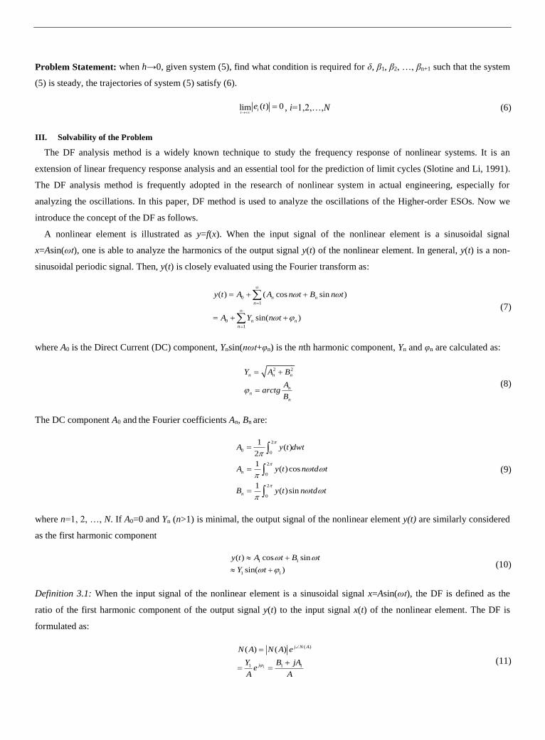
Definition 3.1: When the input signal of the nonlinear element is a sinusoidal signal x=Asin(ωt), the DF is defined as the

ratio of the first harmonic component of the output signal y(t) to the input signal x(t) of the nonlinear element. The DF is

formulated as:

1

( )

1 1 1

( ) ( ) j N A

j

N A N A e

Y B jAe

A A

(11)

To make the problem more trackable, we consider the nonlinear ESO without linearization near zero with the form

fal(e,α,δ)= |e|αsign(e) at first. The nonlinear element is y(x)=|x|αsign(x). y(x) is an odd function of x. When the input signal is

x=Asin(ωt), the derivation and calculation of its DF is presented as y(t)=|Asin(ωt)|αsign(Asin(ωt)), y(t) is an odd function of t.

Therefore, by (9), we can get A0=0, A1=0, B1=g(α)Aα, 12

0

4( ) (sin )g t d t

.

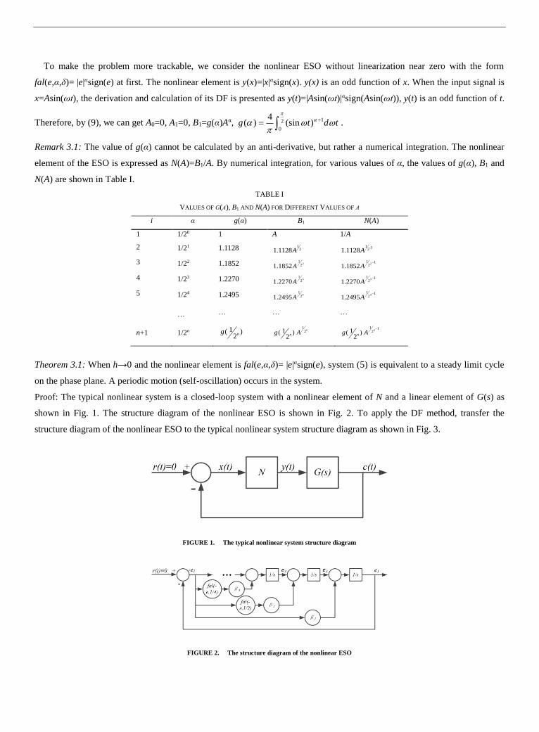
Remark 3.1: The value of g(α) cannot be calculated by an anti-derivative, but rather a numerical integration. The nonlinear

element of the ESO is expressed as N(A)=B1/A. By numerical integration, for various values of α, the values of g(α), B1 and

N(A) are shown in Table I.

TABLE I

VALUES OF G(Α), B1 AND N(A) FOR DIFFERENT VALUES OF Α

i α g(α) B1 N(A)

1 1/20 1 A 1/A

2 1/21 1.1128 121.1128A

1 -121.1128A

3 1/22 1.1852 21

21.1852A 2

1 121.1852A

4 1/23 1.2270 31

21.2270A 3

1 121.2270A

5 1/24 1.2495 41

21.2495A 4

1 121.2495A

…

… … …

n+1 1/2n 1( )2ng

121( )

2

n

ng A 1 1

21( ) 2

n

ng A

Theorem 3.1: When h→0 and the nonlinear element is fal(e,α,δ)= |e|αsign(e), system (5) is equivalent to a steady limit cycle

on the phase plane. A periodic motion (self-oscillation) occurs in the system.

Proof: The typical nonlinear system is a closed-loop system with a nonlinear element of N and a linear element of G(s) as

shown in Fig. 1. The structure diagram of the nonlinear ESO is shown in Fig. 2. To apply the DF method, transfer the

structure diagram of the nonlinear ESO to the typical nonlinear system structure diagram as shown in Fig. 3.

FIGURE 1. The typical nonlinear system structure diagram

FIGURE 2. The structure diagram of the nonlinear ESO

FIGURE 3. The transformed structure diagram of the nonlinear ESO

The transformed structure diagram of the nonlinear ESO is a closed-loop system with a nonlinear element of N and a

linear element of G as shown in Fig. 3. The nonlinear element is illustrated as y(t)=e2=f(-e1). If a self-oscillation occurs in the

system, we can always assume that the input signal of the nonlinear element is complex but close to a sinusoidal signal x(t)=-

e1=Asinωt with time, as the output high-order harmonic components of the nonlinear element N are attenuated by the linear

element G (Friedland, 1996). In this case, the output of the nonlinear element y(t) can be regarded as a non-sinusoidal

periodic signal. The Fourier transform is used to analyze the equation y=e2=f(-e1) as

-1

1

21 -1

2

1( ) ( ) sin( ( 1))

22

kk

k kk

y t g A wt k

(12)

2 2 1

1 1

2 1 22 22 2 2 1 2 1

1 1

1 1( ) ( ( 1) ( ) , ( 1) ( ) )

2 2

k kk kk k

k k k kk k

y t g A g A

(13)

2 2 1

1 11 1

2 1 22 22 2 2 1 2 1

1 1

( ) 1 1( ) ( ( 1) ( ) , ( 1) ( ) )

2 2

k kk kk k

k k k kk k

y tN A g A g A

A

(14)

where, k=1, 2, …, N.

The Negative Converse Describing Function (NCDF) of the nonlinear element is -1/N(A). The Frequency Characteristic

(FC) of the linear element is calculated as 1

1( )G j

j

. The characteristic equation for the nonlinear ESO error function

is expressed as

1( )

( )G j

N A

(15)

Taking the third-order ESOs as an example, the curves of G(jω) and NCDF are shown in the complex plane (where

β1=100, β2=300, β3=1000), as seen in Fig. 4.

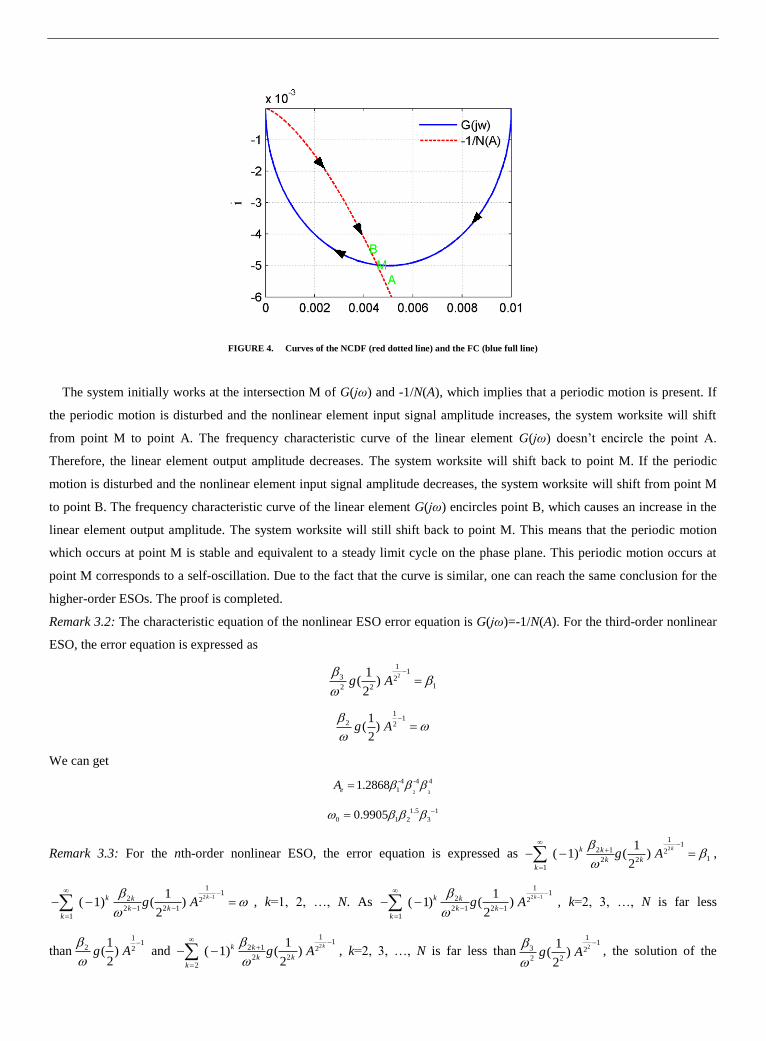
FIGURE 4. Curves of the NCDF (red dotted line) and the FC (blue full line)

The system initially works at the intersection M of G(jω) and -1/N(A), which implies that a periodic motion is present. If

the periodic motion is disturbed and the nonlinear element input signal amplitude increases, the system worksite will shift

from point M to point A. The frequency characteristic curve of the linear element G(jω) doesn’t encircle the point A.

Therefore, the linear element output amplitude decreases. The system worksite will shift back to point M. If the periodic

motion is disturbed and the nonlinear element input signal amplitude decreases, the system worksite will shift from point M

to point B. The frequency characteristic curve of the linear element G(jω) encircles point B, which causes an increase in the

linear element output amplitude. The system worksite will still shift back to point M. This means that the periodic motion

which occurs at point M is stable and equivalent to a steady limit cycle on the phase plane. This periodic motion occurs at

point M corresponds to a self-oscillation. Due to the fact that the curve is similar, one can reach the same conclusion for the

higher-order ESOs. The proof is completed.

Remark 3.2: The characteristic equation of the nonlinear ESO error equation is G(jω)=-1/N(A). For the third-order nonlinear

ESO, the error equation is expressed as

2

11

3 212 2

1( ) 2

g A

11

2 21

( ) 2

g A

We can get

2 3

-4 -4 4

11.2868eA

1.5 1

0 1 2 30.9905

Remark 3.3: For the nth-order nonlinear ESO, the error equation is expressed as 2

11

2 1 212 2

1

1 ( 1) ( )

2

kk k

k kk

g A

,

2 1

11

2 22 1 2 1

1

1 ( 1) ( )

2

kk k

k kk

g A

, k=1, 2, …, N. As 2 1

11

2 22 1 2 1

1

1 ( 1) ( )

2

kk k

k kk

g A

, k=2, 3, …, N is far less

than1

12 2

1( ) 2

g A

and 2

11

2 1 22 2

2

1 ( 1) ( )

2

kk k

k kk

g A

, k=2, 3, …, N is far less than2

11

3 22 2

1( ) 2

g A

, the solution of the

characteristic equation of the third-order nonlinear ESO error function can be considered as the solution of the characteristic

equation of high-order nonlinear ESOs error equation.

For example, when β1=100, β2=300, β3=1000, β4=1800, β5=3000, the solution of the characteristic function of the nth-

ESOs error equation is shown in Table II.

TABLE II

SOLUTION OF THE CHARACTERISTIC EQUATION OF THE NTH-ESO ERROR EQUATION

ESO third-order forth-order fifth-order …

Ae 1.589e-06 1.613e-6/1.565e-6 1.611e-6/1.614e-6 …

ω0 514.68 511.76/517.52 511.83/517.68 …

Next we consider high-order nonlinear ESOs with linearization near zero.

Remark 3.4: the stability problem of the LESO (fal(e,α,δ)=e) has been thoroughly studied (Yoo et al., 2006, 2007; Yang and

Huang, 2009; Zheng et al., 2012). In particular, when h→0, if all of the roots of the characteristic equation

1

0n

n n i

i

i

s s

are in the left half of the complex plane, the LESO is steady and ( ) 0limt

ie t

, i=1, 2, …, n+1.

Theorem 3.2: Define 1i

Li i

, i=1, 2, …, n+1. If δ>Ae (condition 1) and all of the roots of the characteristic equation

1

0n

n n i

Li

i

s s

are in the left half of the complex plane (condition 2), system (5) is steady, the trajectories of system (5)

satisfy (6).

Proof: The nonlinear element in system (5) is calculated as

1 ,( , , )

( ),

e efal e

e sign e e

. By Theorem 3.1, we know that

when the nonlinear element in system (5) is fal(e,α,δ)= |e|αsign(e), a self-oscillation occurs in the system. The amplitude of e1

when self-oscillation is Ae.

The nonlinear ESO is equivalent to the LESO near zero (|e|≤δ), the corresponding parameters are 1i

Li i

, i=1, 2, …,

n+1. By Remark 3.4 we get that if all of the roots of the characteristic equation 1

0n

n n i

Li

i

s s

are in the left half of the

complex plane, the LESO is steady.

To avoid the self-oscillation caused by the nonlinear element of the nonlinear ESO, the value of the linearization range δ

should be larger than the amplitude of e1 when self-oscillation. It is not hard to see that if conditions 1 and 2 are met, system

(5) is steady. The proof is completed.

Theorem 3.2 gives a method that how δ can be selected to avoid the self-oscillation which might occur in high-order

nonlinear ESOs. The parameter δ can be tuned after the parameters β1, β2, …, βn+1 are set. The parameter δ should meet

condition 1 and condition 2 in Theorem 3.2.

The parameter tuning of the nonlinear ESO has always been a difficult problem for the ADRC design. Based on Theorem

3.2, we give a simple and fast parameter tuning method for the nonlinear ESO. The values of the parameters for the nth-order

ESOs are selected as

1-

0ii i

i nC , i=1, 2, …, n (16)

Then in the linearization range

0

i i

Li nC , i=1, 2, …, n (17)

The according characteristic equation is

0 0

0

( ) 0n

i i n i n

n

i

C s s

(18)

It can be seen that all of the roots of the characteristic equation are in the left half of the complex plane. In addition, the

self-oscillation amplitude of nth-order ESO without any linearization near zero is approximately:

4 43

2 1

1.1852 2( ) 0.0117( )1.1128

nA

n

, n≥3

As we can see from Theorem 3.2, the designated nth-order ESOs are stable. The adjustable parameters are ω0 and δ. δ

represents the value of the linearization range. ω0 represents the band-width of the ESO in the linearization range.

IV. Example

In this section, we simulated to verify the stability analysis results in section III. First we showed that if the nonlinear

element in system (4) is fal(e,α,δ)= |e|αsign(e), the actual amplitudes of the observer estimation errors are in accordance with

the theoretical amplitudes of errors when self-oscillation occurs. When β1=100, β2=300, β3=1000, the theoretical amplitude

and phase of the observer estimation errors for third-order ESOs are calculated, as shown in Table III.

TABLE III

AMPLITUDES AND PHASES OF THE OBSERVER ESTIMATION ERROR WHEN SELF-OSCILLATION

variable Theoretical amplitude Theoretical phase

e1 1.589e-06 0

e2 8.329e-04 79.01

e3 0.082 -90

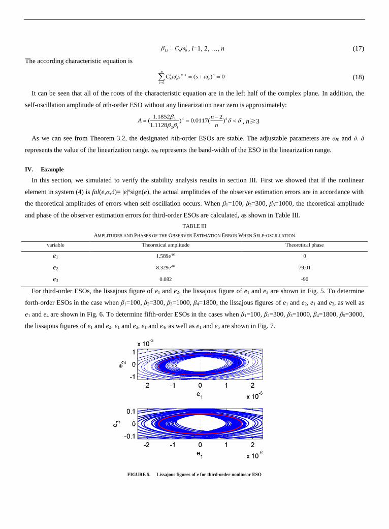
For third-order ESOs, the lissajous figure of e1 and e2, the lissajous figure of e1 and e3 are shown in Fig. 5. To determine

forth-order ESOs in the case when β1=100, β2=300, β3=1000, β4=1800, the lissajous figures of e1 and e2, e1 and e3, as well as

e1 and e4 are shown in Fig. 6. To determine fifth-order ESOs in the cases when β1=100, β2=300, β3=1000, β4=1800, β5=3000,

the lissajous figures of e1 and e2, e1 and e3, e1 and e4, as well as e1 and e5 are shown in Fig. 7.

FIGURE 5. Lissajous figures of e for third-order nonlinear ESO

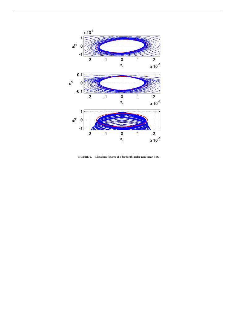
FIGURE 6. Lissajous figures of e for forth-order nonlinear ESO

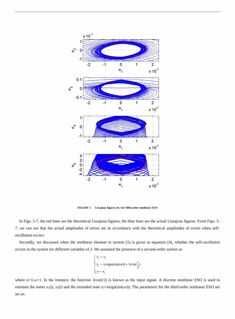
FIGURE 7. Lissajous figures of e for fifth-order nonlinear ESO

In Figs. 5-7, the red lines are the theoretical Lissajous figures; the blue lines are the actual Lissajous figures. From Figs. 5-

7, we can see that the actual amplitudes of errors are in accordance with the theoretical amplitudes of errors when self-

oscillation occurs.

Secondly, we discussed when the nonlinear element in system (5) is given as equation (4), whether the self-oscillation

occurs in the system for different variables of δ. We assumed the presence of a second-order system as

1 2

2

1

sign(sin( )) 3cos( )2

x x

tx a t

y x

where a=1,ω=1. In the instance, the function 3cos(t/2)

is known as the input signal. A discrete nonlinear ESO is used to

estimate the states x1(t), x2(t) and the extended state x3=asign(sin(ωt)). The parameters for the third-order nonlinear ESO are

set as:

β1=100, β2=300, β3=1000

The nonlinear ESO is equivalent to the LESO near zero (|e|≤δ), the corresponding parameters are 1i

Li i

, i=1, 2, …,

n+1. In this case, βL1=β1, 1/2 1

2 2L , 1/ 4 1

3 3L . Based on Theorem 3.2, condition 1 and 2 should be satisfied. For

condition 1, we can get δ>Ae, 2 3

-4 -4 4

11.2868eA . For condition 2, βL1βL2>βL3 should be satisfied. We can get δ>Aβ,

2 3

-4 -4 4

1A . It’s easy to see that when δ>Ae (δ>1.2868Aβ) both condition 1 and 2 are satisfied. To verify Theorem 3.2,

we chose a little smaller value than Ae and a little larger value than Ae for parameter δ. The values of parameter δ for third-

order nonlinear ESO are selected as:

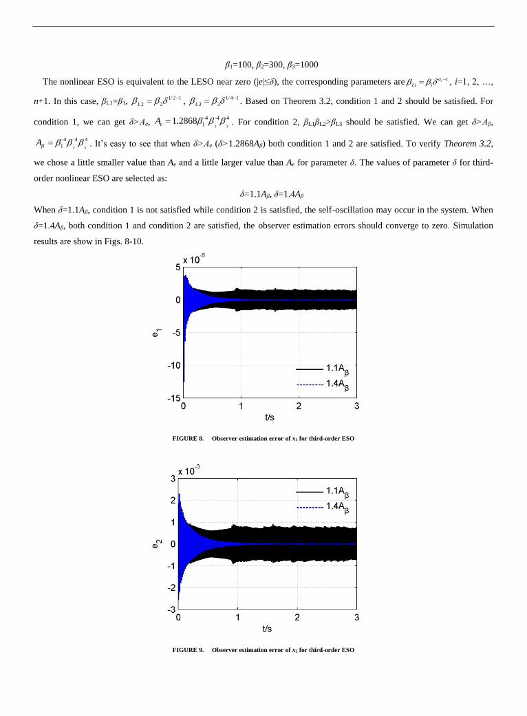
δ=1.1Aβ, δ=1.4Aβ

When δ=1.1Aβ, condition 1 is not satisfied while condition 2 is satisfied, the self-oscillation may occur in the system. When

δ=1.4Aβ, both condition 1 and condition 2 are satisfied, the observer estimation errors should converge to zero. Simulation

results are show in Figs. 8-10.

FIGURE 8. Observer estimation error of x1 for third-order ESO

FIGURE 9. Observer estimation error of x2 for third-order ESO

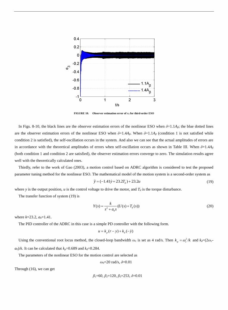
FIGURE 10. Observer estimation error of x3 for third-order ESO

In Figs. 8-10, the black lines are the observer estimation errors of the nonlinear ESO when δ=1.1Aβ; the blue dotted lines

are the observer estimation errors of the nonlinear ESO when δ=1.4Aβ. When δ=1.1Aβ (condition 1 is not satisfied while

condition 2 is satisfied), the self-oscillation occurs in the system. And also we can see that the actual amplitudes of errors are

in accordance with the theoretical amplitudes of errors when self-oscillation occurs as shown in Table III. When δ=1.4Aβ

(both condition 1 and condition 2 are satisfied), the observer estimation errors converge to zero. The simulation results agree

well with the theoretically calculated ones.

Thirdly, refer to the work of Gao (2003), a motion control based on ADRC algorithm is considered to test the proposed

parameter tuning method for the nonlinear ESO. The mathematical model of the motion system is a second-order system as

( 1.41 23.2 ) 23.2dy y T u (19)

where y is the output position, u is the control voltage to drive the motor, and Td is the torque disturbance.

The transfer function of system (19) is

2

0

( ) ( ( ) ( ))d

kY s U s T s

s a s

(20)

where k=23.2, a0=1.41.

The PID controller of the ADRC in this case is a simple PD controller with the following form.

( ) ( )p du k r y k y

Using the conventional root locus method, the closed-loop bandwidth ωc is set as 4 rad/s. Then 2 /p ck k and kd=(2ωc-

a0)/k. It can be calculated that kp=0.689 and kd=0.284.

The parameters of the nonlinear ESO for the motion control are selected as

ω0=20 rad/s, δ=0.01

Through (16), we can get

β1=60, β2=120, β3=253, δ=0.01

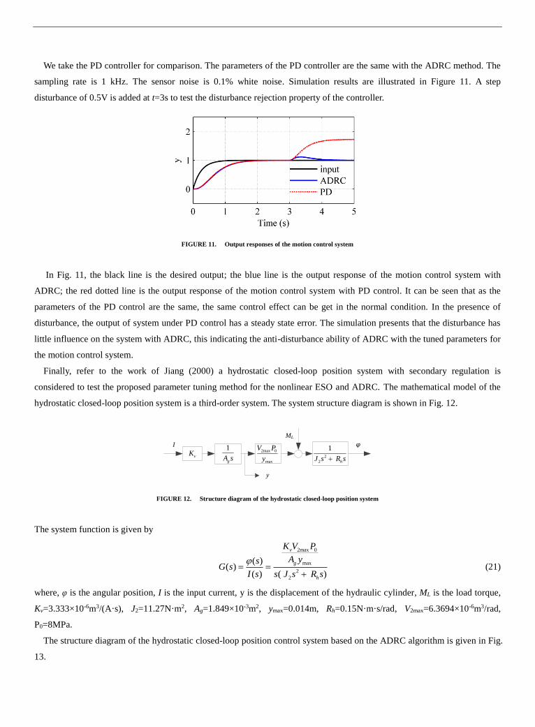
We take the PD controller for comparison. The parameters of the PD controller are the same with the ADRC method. The

sampling rate is 1 kHz. The sensor noise is 0.1% white noise. Simulation results are illustrated in Figure 11. A step

disturbance of 0.5V is added at t=3s to test the disturbance rejection property of the controller.

FIGURE 11. Output responses of the motion control system

In Fig. 11, the black line is the desired output; the blue line is the output response of the motion control system with

ADRC; the red dotted line is the output response of the motion control system with PD control. It can be seen that as the

parameters of the PD control are the same, the same control effect can be get in the normal condition. In the presence of

disturbance, the output of system under PD control has a steady state error. The simulation presents that the disturbance has

little influence on the system with ADRC, this indicating the anti-disturbance ability of ADRC with the tuned parameters for

the motion control system.

Finally, refer to the work of Jiang (2000) a hydrostatic closed-loop position system with secondary regulation is

considered to test the proposed parameter tuning method for the nonlinear ESO and ADRC. The mathematical model of the

hydrostatic closed-loop position system is a third-order system. The system structure diagram is shown in Fig. 12.

ML

I

y

2

2

1

hJ s R s

2max 0

max

V P

y

1

gA s vK

φ

FIGURE 12. Structure diagram of the hydrostatic closed-loop position system

The system function is given by

2max 0

max

2

2

( )( )

( ) ( )

v

g

h

K V P

A ysG s

I s s J s R s

(21)

where, φ is the angular position, I is the input current, y is the displacement of the hydraulic cylinder, ML is the load torque,

Kv=3.333×10-6m3/(A·s), J2=11.27N·m2, Ag=1.849×10-3m2, ymax=0.014m, Rh=0.15N·m·s/rad, V2max=6.3694×10-6m3/rad,

P0=8MPa.

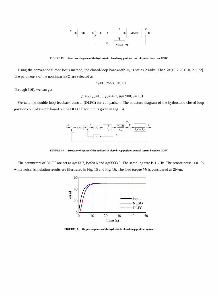
The structure diagram of the hydrostatic closed-loop position control system based on the ADRC algorithm is given in Fig.

13.

Model

I φ

NESO

kTD

_

φ*

z

FIGURE 13. Structure diagram of the hydrostatic closed-loop position control system based on ADRC

Using the conventional root locus method, the closed-loop bandwidth ωc is set as 2 rad/s. Then k=[13.7 20.6 10.2 1.72].

The parameters of the nonlinear ESO are selected as

ω0=15 rad/s, δ=0.01

Through (16), we can get

β1=60, β2=135, β3= 427, β4= 900, δ=0.01

We take the double loop feedback control (DLFC) for comparison. The structure diagram of the hydrostatic closed-loop

position control system based on the DLFC algorithm is given in Fig. 14.

ML

I

y

2

2

1

hJ s R s

2max 0

max

V P

y

1

gA s vKkp+kds

ky

φ* φ

__

FIGURE 14. Structure diagram of the hydrostatic closed-loop position control system based on DLFC

The parameters of DLFC are set as kp=13.7, kd=20.6 and ky=3333.3. The sampling rate is 1 kHz. The sensor noise is 0.1%

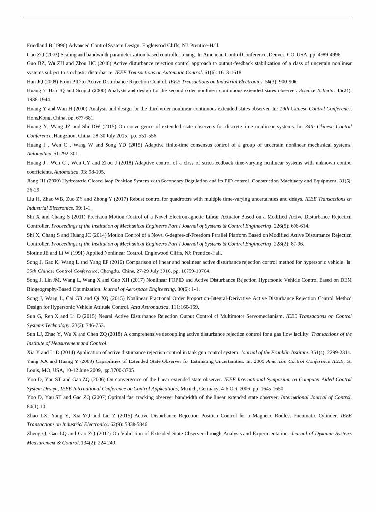
white noise. Simulation results are illustrated in Fig. 15 and Fig. 16. The load torque ML is considered as 2N·m.

FIGURE 15. Output responses of the hydrostatic closed-loop position system

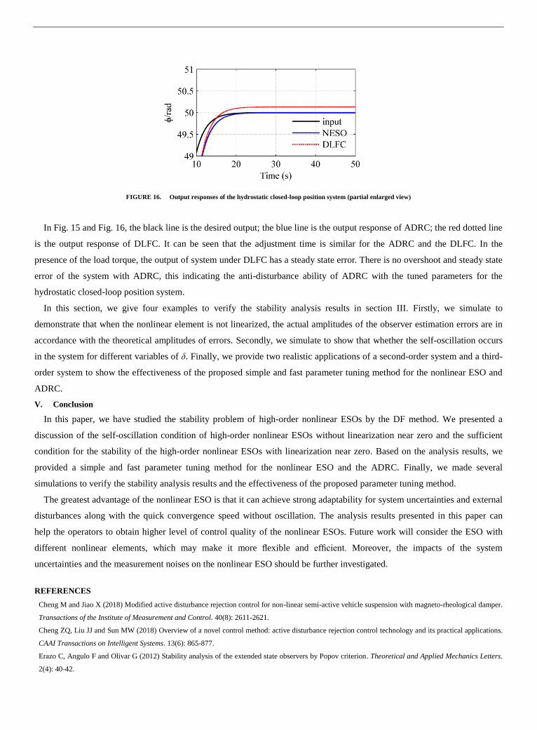
FIGURE 16. Output responses of the hydrostatic closed-loop position system (partial enlarged view)

In Fig. 15 and Fig. 16, the black line is the desired output; the blue line is the output response of ADRC; the red dotted line

is the output response of DLFC. It can be seen that the adjustment time is similar for the ADRC and the DLFC. In the

presence of the load torque, the output of system under DLFC has a steady state error. There is no overshoot and steady state

error of the system with ADRC, this indicating the anti-disturbance ability of ADRC with the tuned parameters for the

hydrostatic closed-loop position system.

In this section, we give four examples to verify the stability analysis results in section III. Firstly, we simulate to

demonstrate that when the nonlinear element is not linearized, the actual amplitudes of the observer estimation errors are in

accordance with the theoretical amplitudes of errors. Secondly, we simulate to show that whether the self-oscillation occurs

in the system for different variables of δ. Finally, we provide two realistic applications of a second-order system and a third-

order system to show the effectiveness of the proposed simple and fast parameter tuning method for the nonlinear ESO and

ADRC.

V. Conclusion

In this paper, we have studied the stability problem of high-order nonlinear ESOs by the DF method. We presented a

discussion of the self-oscillation condition of high-order nonlinear ESOs without linearization near zero and the sufficient

condition for the stability of the high-order nonlinear ESOs with linearization near zero. Based on the analysis results, we

provided a simple and fast parameter tuning method for the nonlinear ESO and the ADRC. Finally, we made several

simulations to verify the stability analysis results and the effectiveness of the proposed parameter tuning method.

The greatest advantage of the nonlinear ESO is that it can achieve strong adaptability for system uncertainties and external

disturbances along with the quick convergence speed without oscillation. The analysis results presented in this paper can

help the operators to obtain higher level of control quality of the nonlinear ESOs. Future work will consider the ESO with

different nonlinear elements, which may make it more flexible and efficient. Moreover, the impacts of the system

uncertainties and the measurement noises on the nonlinear ESO should be further investigated.

REFERENCES

Cheng M and Jiao X (2018) Modified active disturbance rejection control for non-linear semi-active vehicle suspension with magneto-rheological damper.

Transactions of the Institute of Measurement and Control. 40(8): 2611-2621.

Cheng ZQ, Liu JJ and Sun MW (2018) Overview of a novel control method: active disturbance rejection control technology and its practical applications.

CAAI Transactions on Intelligent Systems. 13(6): 865-877.

Erazo C, Angulo F and Olivar G (2012) Stability analysis of the extended state observers by Popov criterion. Theoretical and Applied Mechanics Letters.

2(4): 40-42.

Friedland B (1996) Advanced Control System Design. Englewood Cliffs, NJ: Prentice-Hall.

Gao ZQ (2003) Scaling and bandwidth-parameterization based controller tuning. In American Control Conference, Denver, CO, USA, pp. 4989-4996.

Guo BZ, Wu ZH and Zhou HC (2016) Active disturbance rejection control approach to output-feedback stabilization of a class of uncertain nonlinear

systems subject to stochastic disturbance. IEEE Transactions on Automatic Control. 61(6): 1613-1618.

Han JQ (2008) From PID to Active Disturbance Rejection Control. IEEE Transactions on Industrial Electronics. 56(3): 900-906.

Huang Y Han JQ and Song J (2000) Analysis and design for the second order nonlinear continuous extended states observer. Science Bulletin. 45(21):

1938-1944.

Huang Y and Wan H (2000) Analysis and design for the third order nonlinear continuous extended states observer. In: 19th Chinese Control Conference,

HongKong, China, pp. 677-681.

Huang Y, Wang JZ and Shi DW (2015) On convergence of extended state observers for discrete-time nonlinear systems. In: 34th Chinese Control

Conference, Hangzhou, China, 28-30 July 2015, pp. 551-556.

Huang J , Wen C , Wang W and Song YD (2015) Adaptive finite-time consensus control of a group of uncertain nonlinear mechanical systems.

Automatica. 51:292-301.

Huang J , Wen C , Wen CY and Zhou J (2018) Adaptive control of a class of strict-feedback time-varying nonlinear systems with unknown control

coefficients. Automatica. 93: 98-105.

Jiang JH (2000) Hydrostatic Closed-loop Position System with Secondary Regulation and its PID control. Construction Machinery and Equipment. 31(5):

26-29.

Liu H, Zhao WB, Zuo ZY and Zhong Y (2017) Robust control for quadrotors with multiple time-varying uncertainties and delays. IEEE Transactions on

Industrial Electronics. 99: 1-1.

Shi X and Chang S (2011) Precision Motion Control of a Novel Electromagnetic Linear Actuator Based on a Modified Active Disturbance Rejection

Controller. Proceedings of the Institution of Mechanical Engineers Part I Journal of Systems & Control Engineering. 226(5): 606-614.

Shi X, Chang S and Huang JC (2014) Motion Control of a Novel 6-degree-of-Freedom Parallel Platform Based on Modified Active Disturbance Rejection

Controller. Proceedings of the Institution of Mechanical Engineers Part I Journal of Systems & Control Engineering. 228(2): 87-96.

Slotine JE and Li W (1991) Applied Nonlinear Control. Englewood Cliffs, NJ: Prentice-Hall.

Song J, Gao K, Wang L and Yang EF (2016) Comparison of linear and nonlinear active disturbance rejection control method for hypersonic vehicle. In:

35th Chinese Control Conference, Chengdu, China, 27-29 July 2016, pp. 10759-10764.

Song J, Lin JM, Wang L, Wang X and Guo XH (2017) Nonlinear FOPID and Active Disturbance Rejection Hypersonic Vehicle Control Based on DEM

Biogeography-Based Optimization. Journal of Aerospace Engineering. 30(6): 1-1.

Song J, Wang L, Cai GB and Qi XQ (2015) Nonlinear Fractional Order Proportion-Integral-Derivative Active Disturbance Rejection Control Method

Design for Hypersonic Vehicle Attitude Control. Acta Astronautica. 111:160-169.

Sun G, Ren X and Li D (2015) Neural Active Disturbance Rejection Output Control of Multimotor Servomechanism. IEEE Transactions on Control

Systems Technology. 23(2): 746-753.

Sun LJ, Zhao Y, Wu X and Chen ZQ (2018) A comprehensive decoupling active disturbance rejection control for a gas flow facility. Transactions of the

Institute of Measurement and Control.

Xia Y and Li D (2014) Application of active disturbance rejection control in tank gun control system. Journal of the Franklin Institute. 351(4): 2299-2314.

Yang XX and Huang Y (2009) Capabilities of Extended State Observer for Estimating Uncertainties. In: 2009 American Control Conference IEEE, St.

Louis, MO, USA, 10-12 June 2009, pp.3700-3705.

Yoo D, Yau ST and Gao ZQ (2006) On convergence of the linear extended state observer. IEEE International Symposium on Computer Aided Control

System Design, IEEE International Conference on Control Applications, Munich, Germany, 4-6 Oct. 2006, pp. 1645-1650.

Yoo D, Yau ST and Gao ZQ (2007) Optimal fast tracking observer bandwidth of the linear extended state observer. International Journal of Control,

80(1):10.

Zhao LX, Yang Y, Xia YQ and Liu Z (2015) Active Disturbance Rejection Position Control for a Magnetic Rodless Pneumatic Cylinder. IEEE

Transactions on Industrial Electronics. 62(9): 5838-5846.

Zheng Q, Gao LQ and Gao ZQ (2012) On Validation of Extended State Observer through Analysis and Experimentation. Journal of Dynamic Systems

Measurement & Control. 134(2): 224-240.