powerful nonlinear observer … nonlinear observer associated with field-oriented ... equations...

Int. J. Appl. Math. Comput. Sci., 2004, Vol. 14, No. 2, 209–220

POWERFUL NONLINEAR OBSERVER ASSOCIATED WITH FIELD-ORIENTEDCONTROL OF AN INDUCTION MOTOR

ABDELLAH MANSOURI∗, MOHAMMED CHENAFA∗, ABDERRAHMANE BOUHENNA∗, ERIC ETIEN∗∗

∗ Department of Electrical Engineering, E.N.S.E.T. OranLaboratory of Automatics and Systems Analysis (L.A.A.S.)

BP 1523 El’ M’naouer, Oran, Algeriae-mail:[email protected]

∗∗ Laboratoire d’Automatique et d’Informatique IndustrielleEcole Supérieure d’Ingénieurs de Poitiers, Université de Poitiers

40, Avenue du Recteur Pineau, 86022 Poitiers Cedex, Francee-mail:[email protected]

In this paper, we associate field-oriented control with a powerful nonlinear robust flux observer for an induction motorto show the improvement made by this observer compared with the open-loop and classical estimator used in this typeof control. We implement this design strategy through an extension of a special class of nonlinear multivariable systemssatisfying some regularity assumptions. We show by an extensive study that this observer is completely satisfactory at lowand nominal speeds and it is not sensitive to disturbances and parametric errors. It is robust to changes in load torque,rotational speed and rotor resistance. The method achieves a good performance with only one easier gain tuning obtainedfrom an algebraic Lyapunov equation. Finally, we present results and simulations with concluding remarks on the advantagesand perspectives for the observer proposed with the field-oriented control.

Keywords: induction motor, field-oriented control, nonlinear observer, rotor resistance

1. Introduction

Induction motors are widely used in industry due to theirrelatively low cost and high reliability. One way to ob-tain a speed or torque control with a dynamic perfor-mance similar to that of a more expensive DC-motor isto use Field-Oriented Control (FOC) (Blaschke, 1972;Bekkoucheet al., 1998; Mansouriet al., 1997). Manyother methods have been suggested but, in general, an es-timate of the rotor flux is needed in most of these con-trol schemes. Therefore a rotor flux observer must be em-ployed. The dynamic behaviour of the induction motor isaffected by time variations, mainly in the rotational speedand in the rotor resistance. The rotor flux observer mustbe robust with respect to these variations. The simplestflux estimation method is an open-loop observer basedon stator current measurements (Grellet and Clerc, 1996).This method suffers from poor robustness and a slow con-vergence rate. Several methods have been suggested toovercome this, but most of them are hard to tune or diffi-cult to implement. It is shown in (Gauthier and Bornard,1981) that the major difficulty in implementing the highgain observer comes from the fact that the gain is depen-

dent on the coordinate transformation and it necessitatesthe inversion of its Jacobian. Another approach for de-signing nonlinear observers is to consider the propertiesof ‘richness’ or ‘persistency’ of inputs in the design strat-egy (Bornardet al., 1988). In this respect, Bornard andHammouri (1991) designed an observer for a class of non-linear systems under ’locally regular inputs.’ However,we obtain the gain of the observer from some differentialequations which are not usually desirable for implementa-tion purposes. For industrial purposes, the ideal observerscheme is easy to implement in hardware and does not re-quire tuning.

In this paper a robust flux observer is developed usinga multivariable systems approach (Busawonet al., 1998).The observer does not require any kind of transformationto update its gain and is explicitly obtained from the so-lution of the algebraic Lyapunov equation. As a result,its implementation is greatly facilitated. In the first sec-tion, we present a model of an induction motor and field-oriented control. In the following section, the flux ob-server in both open and closed loops and the proposednonlinear observer are introduced. Finally, a comparisonin simulation between these three estimators is given. The

A. Mansouri et al.210

concluding remarks on the advantages and perspectivesfor the observer proposed with the field-oriented controlare then given.

2. Motor Model and Field-Oriented Control

Modern control techniques often require a state-spacemodel (Van Raumeret al., 1994). The state-space rep-resentation of the asynchronous motor depends on thechoice of the reference frame(α, β) or (d, g) and on thestate variables selected for the electric equations. We writethe equations in the frame(d, g) because it is the mostgeneral and most complex solution, the frame(α, β) be-ing only its one particular case. Nevertheless, the use ofthe frame(d, g) implies exact knowledge of the positionof this frame. The choice of the state variablex dependson the objectives of the control or observation. For a com-plete model, the mechanical speedΩ is a state variable.The outputs to be independently controlled are the normof the rotor flux and the torque. The rotor flux norm needsto be controlled for system optimization (e.g. power ef-ficiency, torque maximization) while changing operatingconditions and under inverter limits (Garciaet al., 1994;Bodson and Chiasson, 1992). Torque control is essentialfor high dynamic performances. Once the torque is con-trolled, the speed and position can be controlled by simpleouter linear loops, at least, if the load does not have sig-nificantly nonlinear dynamics (De Witet al., 1995).

As state variables, we choose the two components ofstator currents, the two components of the rotor flux andthe mechanical speed. As for the outputy, the torque andthe square of the rotor flux norm and for the input volt-age, the stator voltage inputu is selected. We can thenwrite the model equations in the reference frame(d, g)as follows:

x = f(x) + gu (1)

and

y(x) =

pM

Lr(ϕrdisq − ϕrdisd)

ϕ2rd + ϕ2

rd

, (2)

where

x = [isd, isq, ϕrd,Ω]T , u = [usd, usq]T ,

f(x) =

−γisd + ωsisq +K

Trϕrd + pΩKϕrd

−ωisd − γisq − pΩKϕrd +K

Trϕrd

M

Trisd −

1Tr

ϕrd + (ωs − pΩ)ϕrq

M

Trisq − (ωs − pΩ)ϕrd −

1Tr

ϕrq

pM

JmLr(ϕrdisq − ϕrqisd)−

fmΩJm

− τL

Jm

and

g =

1σLs

0 0 0 0

01

σLs0 0 0

T

with

Tr =Lr

Rr, σ = 1− M2

LsLr,

K =M

σLsLr, γ =

Rs

σLs+

RrM2

σLsL2r

.

Lr, Ls and M are the rotor, stator and mutual induc-tances, respectively,Rr and Rs are respectively rotorand stator resistances,σ is the scattering coefficient,Tr

is the time constant of the rotor dynamics,Jm is the rotorinertia, fm is the mechanical viscous damping,p is thepole pair induction, andτL is the external load torque.We describe the induction motor in the stator fixed frame(α, β) with the previous equations by settingωs = 0,which is the pulsation of stator currents, and by replacingthe indices(d, q) by (α, β), respectively. Good charac-teristics of the model(d, q) appear when we choose forθs a particular orientation of the rotor flux such as

ϕrd = 0, with θs =∫ t

0

ωsdτ.

Consider the following feedback nonlinear statewherevd and vq are auxiliary controls inputs:

(usd

usq

)=σLs

−K

Trϕrd−pΩisq−

M

Tr

i2sq

ϕrd+vd

pKΩϕrd+pΩisd+M

Tr

isdisq

ϕrd+vq

. (3)

Consequently, we obtain a simple system, with the dy-namics of the module of linear flux,

ddt

ϕrd = − 1Tr

ϕrd +M

Trisd,

ddt

isd = −γisd + vd.

(4)

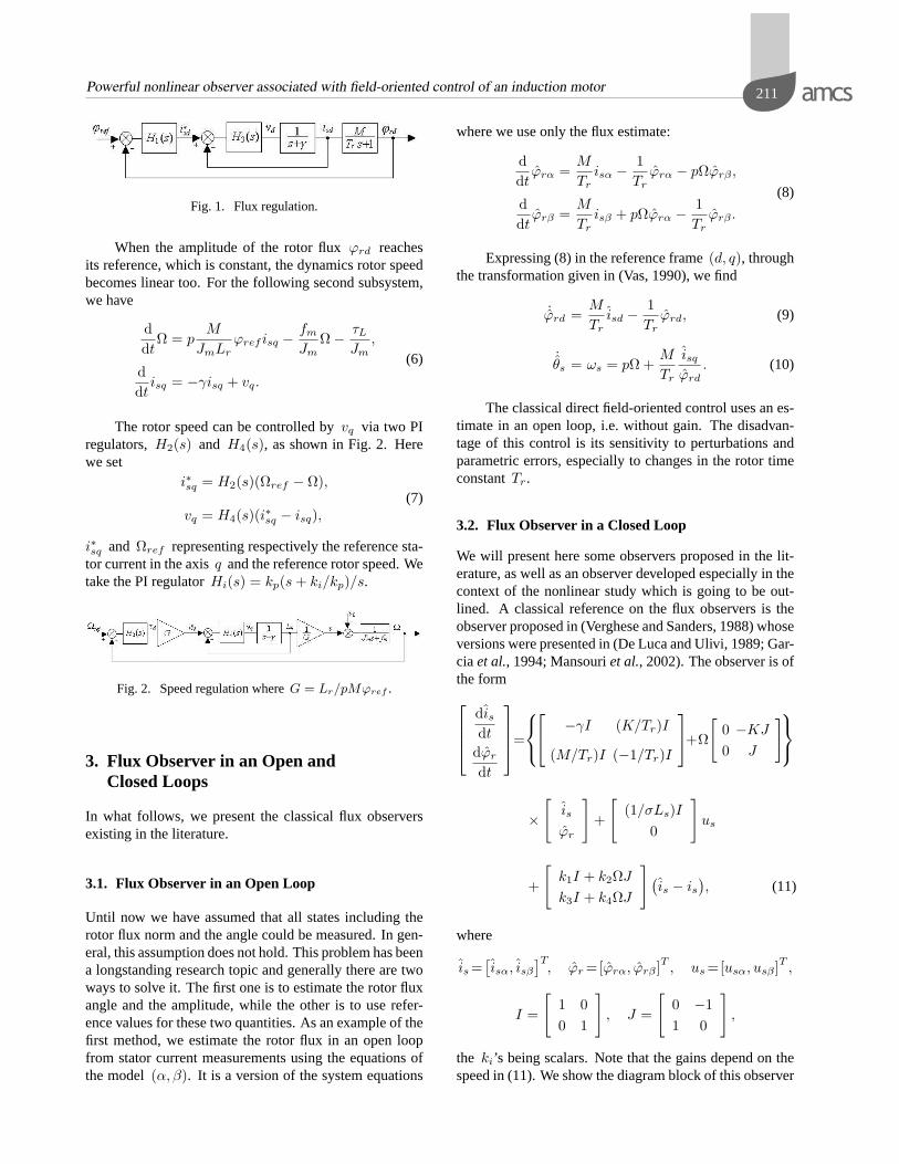
As was shown in (Marinoet al., 1993; Van Raumeretal., 1994), we can control the dynamics of the amplitudeof the flux by vd via two PI regulatorsH1(s) and H3(s)as shown in Fig. 1. Here we set

i∗sd = H1(s)(ϕrerf − ϕrd),

vd = H3(s)(i∗sd − isd),(5)

so thati∗sd and ϕref represent respectively the referencestator current and the reference rotor flux, in the axisd.

Powerful nonlinear observer associated with field-oriented control of an induction motor 211

Fig. 1. Flux regulation.

When the amplitude of the rotor fluxϕrd reachesits reference, which is constant, the dynamics rotor speedbecomes linear too. For the following second subsystem,we have

ddt

Ω = pM

JmLrϕref isq −

fm

JmΩ− τL

Jm,

ddt

isq = −γisq + vq.

(6)

The rotor speed can be controlled byvq via two PIregulators,H2(s) and H4(s), as shown in Fig. 2. Herewe set

i∗sq = H2(s)(Ωref − Ω),

vq = H4(s)(i∗sq − isq),(7)

i∗sq and Ωref representing respectively the reference sta-tor current in the axisq and the reference rotor speed. Wetake the PI regulatorHi(s) = kp(s + ki/kp)/s.

Fig. 2. Speed regulation whereG = Lr/pMϕref .

3. Flux Observer in an Open andClosed Loops

In what follows, we present the classical flux observersexisting in the literature.

3.1. Flux Observer in an Open Loop

Until now we have assumed that all states including therotor flux norm and the angle could be measured. In gen-eral, this assumption does not hold. This problem has beena longstanding research topic and generally there are twoways to solve it. The first one is to estimate the rotor fluxangle and the amplitude, while the other is to use refer-ence values for these two quantities. As an example of thefirst method, we estimate the rotor flux in an open loopfrom stator current measurements using the equations ofthe model(α, β). It is a version of the system equations

where we use only the flux estimate:

ddt

ϕrα =M

Trisα −

1Tr

ϕrα − pΩϕrβ ,

ddt

ϕrβ =M

Trisβ + pΩϕrα −

1Tr

ϕrβ .

(8)

Expressing (8) in the reference frame(d, q), throughthe transformation given in (Vas, 1990), we find

˙ϕrd =M

Trisd −

1Tr

ϕrd, (9)

˙θs = ωs = pΩ +

M

Tr

isq

ϕrd. (10)

The classical direct field-oriented control uses an es-timate in an open loop, i.e. without gain. The disadvan-tage of this control is its sensitivity to perturbations andparametric errors, especially to changes in the rotor timeconstantTr.

3.2. Flux Observer in a Closed Loop

We will present here some observers proposed in the lit-erature, as well as an observer developed especially in thecontext of the nonlinear study which is going to be out-lined. A classical reference on the flux observers is theobserver proposed in (Verghese and Sanders, 1988) whoseversions were presented in (De Luca and Ulivi, 1989; Gar-ciaet al., 1994; Mansouriet al., 2002). The observer is ofthe form

disdt

dϕr

dt

=

−γI (K/Tr)I

(M/Tr)I (−1/Tr)I

+Ω

[0 −KJ

0 J

]

×

[is

ϕr

]+

[(1/σLs)I

0

]us

+

[k1I + k2ΩJ

k3I + k4ΩJ

] (is − is

), (11)

where

is =[isα, isβ

]T, ϕr =[ϕrα, ϕrβ ]T , us =[usα, usβ ]T ,

I =

[1 00 1

], J =

[0 −11 0

],

the ki’s being scalars. Note that the gains depend on thespeed in (11). We show the diagram block of this observer


Fig. 3. Closed-loop observer block diagram.

in Fig. 3. The resulting model for the observer error dy-namics is then

de

dt=

[(k1 − γ)I (K/Tr)I

[k3 + (M/Tr)I] (−1/Tr)I

]

+ Ω

[k2J −KJ

k4I J

]e, (12)

where

e =

[is − is

ϕr − ϕr

].

Note that we can freely determine the scalar coeffi-cients in the left-hand blocks of the two matrices in (12).If k1 and k3 are selected such that

k1 − γ = −k2

Tr, k3 +

M

Tr= −k4

Tr,

the error dynamics become

de

dt= AQ(Ω)e,

where

A =

[k2I −KI

k4I I

],

Q(Ω) =

(− 1

Tr

)I + ΩJ 0

0(− 1

Tr

)I + ΩJ

.

We selectk1 and k4 to place the eigenvalues ofAin arbitrary positions. Note that the characteristic polyno-mial of A is [p2 − (1 + k2)p + k2 + k4K]2.

If the eigenvalues ofA are p1 (twice) and p2

(twice), then the eigenvalues ofAQ(Ω) are

[(−1/Tr)± jΩ] p1, [(−1/Tr)± jΩ] p2. (13)

4. Observer Design for a Special Class ofNonlinear Systems

We present now extensions of the observer design strategyto the multi-output case (Busawonet al., 1998; Chenafaetal., 2002) and an application to the induction motor.

4.1. Extensions of the Observer Design Strategy to theMulti-Output Case

In this section, we show how the previous observer de-signs can be extended to a class of multi-output systemswhich may assume stronger nonlinear dependencies onstate variables. Consider multi-output systems of the fol-lowing form:

z1 = F1(s, y)z2 + g1(u, s, z1),z2 = F2(s, y)z3 + g2(u, s, z1, z2),

...

zn−1 = Fn−1(s, y)zn + gn−1(u, s, z1, . . . , zn−1),zn = gn(u, s, z),y = z1,

(14)where

zl ∈ Rq, l = 1, . . . , n, z =

z1

...

zn

∈ Rn×q,

u ∈ Rm, y ∈ Rq and s(t) is a known signal.Fl are q×q square matrices andgl = (gl1, . . . , glq), l = 1, . . . , n.

We can write the system (14) in the following com-pact form:

z = F (s, y)z + G(u, s, z),y = Cz,

(15)

where

F (s, y) =

0 F1(s, y) 0...

...

Fn−1(s, y)0 . . . . . . 0

,

G(u, s, z) =

g1(u, s, z)...

gn(u, s, z)

, C = [Iq, 0, . . . , 0],

C is of appropriate dimensions andIq is the (q × q)identity matrix.

We note that unlike in the previous sections, eachof the matricesFl, l = 1, . . . , n − 1 now stands for


any square matrix satisfying the assumptions below. Thenonlinearities are block triangular and each block has thesame dimensionq. Also, all the outputs are regrouped inthe first subsystem. Note that the block-triangular struc-ture of the system (14) allows stronger coupling betweenthe nonlinearities, for which the triangular coupling isfound within each subsystem. To see this, consider thesystem

z11 = f11(y)z21 + f12(y)z22,

z12 = f21(y)z21 + f12(y)z22,

z21 = g21(z),z22 = g22(z),y1 = z11,

y2 = z12.

Here, we make the following assumptions:

(A1) There exists a classU of bounded admissible con-trols, a compact setK ⊂ Rn×q and positive con-stantsα, β > 0 such that for everyu ∈ U andevery outputy(t) associated withu and with aninitial state z(0) ∈ K, we have 0 < αIq ≤FT

l (s, y)Fl(s, y) ≤ βIq, l = 1, . . . , n− 1.

(A2) s(t) and its time derivativeds(t)/dt are bounded.

(A3) The matricesFl(s, y), l = 1, . . . , n − 1 are ofclassCr, r ≥ 1 with respect to their arguments.

(A4) The functionsgl, l = 1, . . . , n are global Lips-chitz with respect toz uniformly in u and s.

We characterize the observer design for the sys-tem (15) in the following theorem (Busawonet al., 1998).

Theorem 1.Assume that the system (15) satisfies Assump-tions (A1) to (A4). Then there existsθ > 0 such that thesystem

˙z = F (s, y)z + G(u, s, z)

− Λ−1(s, y)S−1θ CT (Cz − y) (16)

is an exponential observer for the system (15), where

• Sθ is the unique solution of the algebraic Lyapunovequation

θSθ + AT Sθ + SθA− CT C = 0 (17)

with θ > 0 as a parameter, and

A =

0 Iq 0...

...

Iq

0 . . . . . . 0

r,

• the matrixΛ(s, y) is defined as

Λ(s, y) =

C

CF (s, y)...

CFn−1(s, y)

=

Iq 0F1(s, y)

F1(s, y)F2(s, y)...

0n−1∏l=1

Fl(s, y)

.

Moreover, we can make the dynamics of this observerarbitrarily fast (Busawon et al., 1998).

However, we carry out all the computations in ablock-wise fashion, based essentially on the followingfacts: F (s, y) = Λ−1(s, y)AΛ(s, y) and CΛ(s, y) = C.So, by multiplying the left- and right-hand sides of (17)by ΛT (s, y) and Λ(s, y) respectively, the following al-gebraic equation holds:

θSθ(s, y) + FT (s, y)Sθ(s, y)

+Sθ(s, y)F (s, y)− CT C = 0, (18)

where

Sθ = ΛT (s, y)SθΛ(s, y).

Note that the closed-form solution of (18) is

Sθ(i, j) =(−1)i+jCj−1

i+j−2

θi+j−1Iq, 1 ≤ i, j ≤ n. (19)

We can show the diagram block of this observer inFig. 4.

Fig. 4. Nonlinear observer diagram.


4.2. Application to the Induction Motor

In this section, we are going to apply the result given in thepreceding part to construct a reduced flux observer for aninduction motor written in theα, β Park frame. The pro-posed observer uses the measurements of the stator volt-age and current, and the rotor speed. More precisely, theobserver is designed up to an injection of the speed mea-surements so that only electrical equations are considered.As will be seen below, the model is of the form givenby (14). Consequently, the gain can be updated directly,as described in the theorem, without making use of anykind of transformation.

Consequently, the system (15) is of the form (14),wheren = q = 2. We have

z = F (Ω)z + G(u, Ω, z),y = Cz,

(20)

where

z1 =

[isα

isβ

], z2 =

[ϕrα

ϕrβ

], u =

[usα

usβ

],

y =

[isα

isβ

], s = Ω, F1(Ω)=

K

TrKpΩ

−KpΩK

Tr

,

g1(u, Ω, z1) =

−γisα +1

σLsusα

−γisβ +1

σLsusβ

and

g2(u, Ω, z) =

M

Trisα −

1Tr

ϕrα − pΩϕrβ

M

Trisβ + pΩϕrα −

1Tr

ϕrβ

.

Now, assume that the speed and its time derivativesare bounded. Then Assumptions (A1) to (A4) can easilybe checked. Hence we design an observer of the form (16)for the system (20) in Eqn. (21):

˙z = F (Ω)z + G(u, Ω, z)− Λ−1(Ω)S−1θ CT (Cz − y),

(21)where

Λ(Ω) =

[I2 00 F1(Ω)

],

S−1θ CT =

[2θI2

θ2I2

].

The choice ofθ permits the pole placement of themotor and the observer according to the speed.

5. Simulation Results

We have performed simulations using Matlab-Simulinkon the benchmark of Fig. 9 and the motor parametersgiven in Table 1. We studied the performances of the threeobservers in open and closed loops associated with field-oriented control of the induction motor with an increaseof 200% on the rotor constantTr.

Table 1. Parameters of the induction motor.

Parameter Notation Value

Rotor resistance Rr 4.3047Ω

Stator resistance Rs 9.65Ω

Mutual inductance M 0.4475 H

Stator inductance Ls 0.4718 H

Rotor inductance Lr 0.4718 H

Rotor inertia Jm 0.0293 kg/m2

Pole pair p 2

Viscous frictionfm 0.0038 N·m·sec·rad−1

coefficient

5.1. Simulations Block Diagrams, Motor Data anda Benchmark

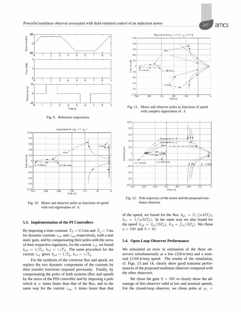
We have designed block diagrams, as shown in Figs. 5–8. The parameters of the induction motor used in simula-tion (Cauët, 2001) are given in Table 1. The trajectoriesof the references speed, flux and load torque are given inFig. 9. This benchmark shows that the load torque appearsat the nominal speed. In spite of a varying speed, the re-sistive torque is zero. The desired flux remains constant inthe asynchronous machine to satisfy the objectives of thefield-oriented control.

5.2. Motor and Observer Poles Dependingon the Speed

In the first case, we consider a closed-loop observer. Thebehaviour of the observers varies considerably depend-ing on whether the eigenvalues are real (Verghese andSanders, 1988) or complex (De Luca, 1989; Belliniet al.,1988). Indeed, in the latter case, the convergence speed,which is a function of the speed and the damping ratio, canbe improved. To illustrate this, we simulated the trajectoryof the poles of the motor and the observer, cf. (11), by tak-ing account of the experimental values given in Section 5.We took real polesp1 = 0.7 and p2 = 1 in Fig. 10, andcomplex polesp1 = 1 + 0.15j and p2 = 0.5 + 0.2j inFig. 11.


Fig. 5. General block diagram in Simulink.

Fig. 6. Induction motor in Simulink.


Fig. 7. Control block in Simulink.

Fig. 8. Observer block in Simulink.

In the second case, we simulated the pole placementof the motor and the observer as a function of the speedresulting of the choice ofθ. For example, the values of

θ equal to three and five were selected for simulations ofFig. 12.


Fig. 9. Reference trajectories.

Fig. 10. Motor and observer poles as functions of speedwith real eigenvalues ofA.

5.3. Implementation of the PI Controllers

By imposing a time constantTd = 0.3 ms andTq = 5 msfor dynamic currentsisd and isq, respectively, with a unitstatic gain, and by compensating their poles with the zerosof their respective regulators, for the currentisd we foundkp3 = 1/Td, ki3 = γ/Td. The same procedure for thecurrent isq gives kp4 = 1/Tq, ki4 = γ/Tq.

For the synthesis of the corrector flux and speed, wereplace the two dynamic components of the currents bytheir transfer functions imposed previously. Finally, bycompensating the poles of both systems (flux and speed)by the zeros of the PID controller and by imposing a polewhich is a times faster than that of the flux, and in thesame way for the currentisq, b times faster than that

Fig. 11. Motor and observer poles as functions of speedwith complex eigenvalues ofA.

Fig. 12. Pole trajectory of the motor and the proposed non-linear observer.

of the speed, we found for the fluxkp1 = Tr/(aMTd),ki1 = 1/(aMTd). In the same way we also found forthe speedkp2 = Jm/(bTq), ki2 = fm/(bTq). We chosea = 100 and b = 10.

5.4. Open-Loop Observer Performance

We simulated an error in estimation of the three ob-servers simultaneously at a low (230 tr/mn) and a nom-inal (1500 tr/mn) speed. The results of the simulation,cf. Figs. 13 and 14, clearly show good transient perfor-mances of the proposed nonlinear observer compared withthe other observers.

We chose the gainθ = 500 to clearly show the ad-vantage of this observer valid at low and nominal speeds.For the closed-loop observer, we chose poles atp1 =


p2 = 2 in the nominal case, to obtain good dynamicsat a nominal speed and to suppress the transitory mode.On the other hand, only one adjustment ofθ enables usto obtain good performances within the range of the speedvariation. The test permits to simulate the convergence ofthe three observers with different values from the actualvalues of the flux in the motor (variation of1 Wb in theflux).

5.5. Performances of the Observers Associated withthe Field-Oriented Control

Tracking speedThe magnitude of the error speed is lowest in the case ofthe nonlinear observer associated with the field-orientedcontrol. Its sign is opposed to the sign of the load torque.Peaks appear at the times of4.2 sec and8.4 sec, i.e.

Fig. 13. Observation errors of the flux at a low speed of230 tr/mn.

Fig. 14. Observation errors of the rotor flux at a nominalspeed (1500 tr/mn).

at the times of the change in the speed sign as shown inFig. 15.

TorqueBetweent = 0 and 0.8 sec, during the linear growth ofthe speed, the load torque corresponds to better dampingfor the nonlinear observer with the control, whereas theresistive torque is zero. Betweent = 0.8 and 3.2 sec, thespeed is constant and the motor torque follows the loadtorque, no matter whether it is zero or equal to20 N·m.The cycle begins again between4 and 9 sec in the oppo-site direction as shown in Fig. 16.

Flux estimation errorAt a constant speed and zero torque, we note the cancel-lation of the observation error. On the other hand, theeffect of the load torque appears in Fig. 17 between1.5and 2.5 sec and between5.5 and 6.5 sec where the flux

Fig. 15. Comparison of the error speed for200% variationin Tr, at θ = 50, p1 = p2 = 2.

Fig. 16. Motor and load torques of field-oriented control.


estimation error has a non-zero constant value. A peakappears when the speed is zero. The nonlinear observershows the best characteristics.

Stator current normWe note that the norm of the stator currents is significantwhen a couple of loads are applied. A peak also appearswhen the speed changes the sign. The amplitude of thiscurrent norm is least significant and of a smooth form forthe nonlinear observer, as shown in Fig. 18.

6. Conclusion

We have proposed a nonlinear observer of a special classassociated with field-oriented flux control. The evaluationregarding the robustness of its performances com-pared with the traditional estimator in an open loop and

Fig. 17. Errors in flux estimation.

Fig. 18. Currents norm stator.

the observer in a closed loop was made when the rotorresistance varied considerably. The results show that thisnonlinear observer offers better performances while track-ing the torque, speed and estimating the flux. It presentsonly one adjustment of the gain in the range of the varyingspeed and it is easy to control, compared with that pro-posed in the closed loop, which requires the adjustment oftwo gains under the constraint on the speed at low valuesor in the nominal case. A major advantage of the methodis that very little tuning was required to obtain the con-vergence of the observation at low speeds. We hope toperform experiments on-line to validate these theoreticalresults.

References

Blaschke F. (1972):The principle of field orientation as appliedto the new transvector closed loop control system for rotat-ing field machines. — Siemens Rev., Vol. XXXIX, No. 5,pp. 217–220.

Bekkouche D., Chenafa M., Mansouri A. and Belaidi A. (1998):A nonlinear control of robot manipulators driven by induc-tion motors. — Proc. 5th Int. WorkshopAdvanced MotionControl, AMC’98, Coimbra University, Coimbra, Portu-gal, pp. 393–398.

Bellini, A., Figalli, G and Ulivi, G. (1988):Analysis and designof a microcomputer based observer for induction machine.— Automatica Vol. 24, No. 4, pp. 549–555.

Bodson M. and Chiasson J. (1992):A systematic approach forselecting optimal flux references in induction motors. —Proc. IEEE IAS Annual Meeting, Houston, TX, USA,pp. 531–537.

Bornard G., Couennen N. and Cell F. (1988):Regularly Persis-tent Observers for Bilinear Systems. — Berlin: Springer.

Bornard G. and Hammouri, H. (1991):An observer for a class ofnonlinear systems under locally regular inputs. — Techn.Rep., Laboratoire d’Automatique de Grenoble, St Martind’Héres, France.

Busawon K., Farza M. and Hammouri H. (1998):Observer de-signs for a special class of nonlinear systems. — Int. J.Contr., Vol. 71, No. 3, pp. 405–418.

Chenafa M., Mansouri A. and Bouhenna A. (2002):Commandelinéarisante avec un observateur d’une classe spécialede systemes non linéaire: Application a un moteur asyn-chrone. — Proc. 4th Int. Conf.Applied Mathematics andEngineering Sciences, Faculty of Sciences, Ain-Chock,Casablanca, Morocco, book of abstracts, p. 85.

Cauët S (2001):Contribution a l’analyse et la synthése de loisde commande robustes pour la machine asynchrone. —Ph. D. thesis, Université de Poitiers, École Supérieured’Ingénieurs de Poitiers, École Doctorale des Sciencespour l’Ingénieur, France.


De Luca A. and Ulivi, G. (1989):Design of an exact nonlinearcontroller for induction motors. — IEEE Trans. Automat.Contr., Vol. 34, No. 12, pp. 1304–1307.

De Wit P., Ortega P.R. and Mareels I. (1995):Indirect field ori-ented control of induction motors, is robustly globally sta-ble. — Proc. 34th IEEE Conf.Decision and Control, NewOrleans, LA, pp. 2139–2144.

Garcia G.O., Mendes Luis J.C., Stephan R.M. and WatanabeE.H. (1994): An efficient controller for an adjustablespeed induction motor drive. — IEEE Trans. Ind. Elec-tron., Vol. 41, No. 5, pp. 533–539.

Gauthier J.P. and Bornard G.(1981):Observability for anyu(t)of a class of nonlinear systems. — IEEE Trans. Automat.Contr., Vol. AC, No. 26, pp. 922–926.

Grellet G. and Clerc G. (1996):Actionneurs électriques.Principes. Modeles. Commandes. — Paris: Eyrolles.

Mansouri A., Chenafa A., Bekkouche D. and Belaidi A. (1997):Sliding Mode Control design and Application to robot ma-nipulator Trained by Induction motors. — Proc. IEEA Int.Annual ConferenceElectronic Engineering, Control En-gineering, Vol. 2, IEEA’97, University of Batna, Algeria,pp. 31–35.

Mansouri A., Belaidi A., Chenafa M. and Bouhenna A. (2002):Commande passive avec observateur non linéaire de lamachine asynchrone. — Proc. 4th Int. Conf.AppliedMathematics and Engineering Sciences, Faculty of Sci-ences Ain-Chock, Casablanca, Morocco, book of ab-stracts, p. 159.

Marino R., Peresada S. and Valigi P. (1993):Adaptive input-output linearizing control of induction motors. — IEEETrans. Automat. Contr., Vol. 38, No. 2, pp. 208–221.

Van Raumer T., Dion J.M., Dugard L. and Thomas J.L. (1994):Applied nonlinear control of an induction motor using dig-ital signal processing. — IEEE Trans. Contr. Syst. Tech-nol., Vol. 2, No. 4, pp. 327–335.

Vas P. (1990): Vector Control of AC Machines. — Oxford:Clarendon Press.

Vas P. (1998):Sensorless vector and direct torque control. —Oxford: Oxford University Press.

Verghese G.C. and Sanders S.R. (1988):Observers for flux esti-mation in induction machines. — IEEE Trans. Ind. Elec-tron., Vol. 35, No. 1, pp. 85–94.

Received: 8 November 2003Revised: 3 February 2004

powerful nonlinear observer … nonlinear observer associated with field-oriented ... equations...

Documents