40, 195’5 observer design for nonlinear systems with...

IEEE TRANSACTIONS ON AUTOMATIC CONTROL, VOL. 40, NO. 3, MARCH 195’5 395

Observer Design for Nonlinear Systems with Discrete-Time Measurements

P. E. Moraal and J. W. Grizzle, Senior Member, ZEEE

Abstract-This paper focuses on the development of asymptotic observers for nonlinear discrete-time systems. It is argued that instead of trying to imitate the linear observer theory, the problem of constructing a nonlinear observer can be more fruitfully studied in the context of solving simultaneous nonlinear equations. In particular, it is shown that the discrete Newton method, properly interpreted, yields an asymptotic observer for a large class of discrete-time systems, while the continuous Newton method may be employed to obtain a global observer. Further- more, it is analyzed how the use of Broyden’s method in the observer structure affects the observer’s performance and its computational complexity. An example illustrates some aspects of the proposed methods; moreover, it serves to show that these methods apply equally well to discrete-time systems and to continuous-time systems with sampled outputs.

I. INTRODUCTION

A. General HE need to study state estimators T namical systems is, from a control

(observers) for dy- point of view, well

understood by now. For the class of finite-dimensional, time- invariant linear systems, a solution to the observer problem has been known since the mid 1960’s: the observer incorporates a copy of the system and uses output injection to achieve an exponentially decaying error dynamics. For the class of continuous-time nonlinear systems, the reader is referred to [38], [39] and the references therein for a summary of the theory up to 1986. More recent developments include the work of Krener et al. [23] on higher-order approximations for achieving a linearizable error dynamics. Tsinias in [37] has proposed (nonconstructive) existence theorems on nonlinear observers via Lyapunov techniques. Gauthier et al. [12] and Deza et al. [9] show how to construct high-gain, extended Luenberger- and Kalman-type observers for a class of nonlinear continuous-time systems. Tomamb2 [36] and Nicosia et al. [31] have proposed a continuous-time version of Newton’s algorithm as a method for computing the inverse kinematics of robots; moreover, the latter paper also presents a symbiotic relationship in general between asymptotic observers and

Manuscript received April 23, 1993; revised May 15, 1994. Recommended by Associate Editor, W. P. Dayawansa. This work was supported in part by National Science Foundation Contract NSF ECS-88-96136.

P. E. Moraal was with Department of Electrical Engineering and Computer Science, University of Michigan at Ann Arbor, MI and is now with Ford Motor Company’s Research Laboratory, Dearbom, MI, 48121-2053 USA.

J. W. Grizzle is with the Department of Electrical Engineering and Computer Science, University of Michigan at Ann Arbor, MI 48109-2122 USA.

IEEE Log Number 9408270.

nonlinear map inversion. Finally, Michalska and Mayne [27] have used a dual form of moving horizon control to construct observers for nonlinear systems.

Less attention has been focused on the observer problem for discrete-time systems. It was shown in [6] that certain properties, like observer error linearizability [22], are not inherited from the underlying continuous-time system. Moreover, the class of continuous-time systems that admit approximate solutions to the observer error linearization problem for their exact discretizations with sampling time T in an open interval is limited to the class of nonlinear systems that are approximately state-equivalent to a linear system and hence is very restricted [5]. These results motivated the search for a structurally more robust approach to the observer problem. In Section 11, it is argued that instead of trying to imitate the linear observer theory, the nonlinear observer problem should be studied in the context of solving sets of simultaneous nonlinear equations. This viewpoint is supported by showing in Section I11 that the discrete Newton method, properly interpreted, yields an asymptotic observer for a large class of discrete-time systems. In Section IV, a relationship between this observer and the well-known extended Kalman filter is established. As an extension to the result from Section 111, it is shown in Section V, that the continuous Newton method may be used to obtain a global exponential observer. Section VI addresses an alternative to using Newton’s method in the observer design-namely, Broyden’s method-in the case that computational efficiency is an important issue. Finally, an example will illustrate the theory presented herein.

Some of the results reported here have previously appeared in [16], [17], and [28]. Extensions to the case of singularly perturbed discrete-time systems have been presented by Shouse and Taylor [33].

B. Notation and Terminology Consider a continuous-time system

where z E R”, U E E”, and y E Rp. Its sampled-data representation, obtained by holding the input constant over half open intervals [kT, (k + 1)T] and measuring the output at times kT, will be denoted

0018-9286/95$04.00 0 1995 IEEE

7 1 7 1 1

Authorized licensed use limited to: University of Michigan Library. Downloaded on June 25, 2009 at 14:22 from IEEE Xplore. Restrictions apply.

. .

396 IEEE TRANSACTIONS ON AUTOMATIC CONTROL, VOL. 40, NO. 3, MARCH 1995

where x k := x ( k T ) , Yk := y ( k T ) , and 'thk := U ( k T ) . The symbol ":=" means that the object on the left is defined to be equal to the object on the right; the reverse holds for "=:."

It is worth noting that if (A,B,C,D) are the matrices describing the Jacobian linearization of (1) around a given equilibrium point, then (exp(AT), Jz exp(A.r) BdT, C, 0) are the corresponding matrices for (2) about the same equilibrium point [14]. Consequently, if the linearization of (1) is controllable and/or observable, the same will be true of the linearization of (2) for "almost all" T [35].

A discrete-time system will be denoted as

arises from a continuous-time system (l), (7) can be obtained directly from (1) by sampling the inputs and outputs N-times faster than the state; in other words, 2j := x ( j N T ) , f i i = ~ ( ( j - 1)NT + iT), etc. More generally, one could sample the inputs and outputs at different rates, or even some input components at faster rates than others, but we will not pursue this here. Throughout this paper, the notation 11 will be used to denote both a vector norm and the corresponding induced operator norm. Finally, we recall that if g: R" + R" is at least once continuously differentiable, its rank at a point z o E R" is the rank of its Jacobian matrix at 20, [4] that is, rank [%(zo)].

U. OBSERVERS FOR SMOOTH where z E R", U E R", and y E Rp. It is convenient to let F"(z) := F ( X , U ) and h"(x) := h(x ,u) so that things like F ( F ( x , u ~ ) , u ~ ) and h ( F ( X , u l ) , u z ) can be written as

DISCRETE-TIME NONLINEAR SYSTEMS

A. General F"2 OF"' ( x ) and hUz OF"' ( x ) respectively, where ''0" denotes composition. Consider a discrete-time system on R"

In the sequel, we will often be dealing with a set of N consecutive measurements or controls; these will be denoted as

If N is fixed and clearly understood, then the abbreviations Y k and will be employed, so that certain formulas will be easier to read.

To a discrete-time system E, we associate an N-lifted system (see [ll]), E N , by block processing the measurements and controls over a window of N sampling instances. Specifically, fix N and let := Y N ~ = q N ( j - l ) + l , N i ] ,

in terms of its vector components as Oj = col(iijl, . . . , iij") where 6: := U N ( j - l ) + i . Let

Oj := U N j = U [ N ( j - l ) + l , N j ] , and 2j := X N j . write Out uj

@(2, O) := FGN o * * . o FG1 ( 2 )

and

The N-lifted system is defined to be

Note that its dynamics is nothing more than the dynamics of (3) iterated N-times. The state of (7) is the state of (3) at the beginning of each "window" of length N , and @ simply describes how the state evolves from window to window. The representation (7) can be termed "multirate" because, if (3)

with Zk E R', some z 2 0, is an asymptotic observer [25] for (8) if it satisfies: A) V x 1 E R " , V U ~ E R", 3 z 1 E R'

R", z 1 E B', limk,, Il?k - xk11 = 0. If the read-out map q in (9) is the identity, ?k = Zk, then (9) is called an identity observer [25]; if the convergence of ? to x is exponential, then (9) is called an exponential observer.

For later use, the observer (9) will be said to be dead-beat

such that ?k = x k for all k 2 2, and B) v x l E Rn,vuk E

Of order d, if, upon Writing r ( Z k , Y k , U k ) =: r Y k r u k ( Z k ) and q ( Z k , Y k , U k ) =: Q Y k r U k ( z k ), then

independently of the particular observer initial condition 2 1 ,

where z d is the state of (8) at time d. It is remarked that dead-beat observers are of interest for stabilization problems, because, if Uk = ( . ( x k ) is a stabilizing feedback for (8), then Uk = a!(?k) will always result in an internally stable closed-loop system whenever the observer (9) has the dead- beat property. This is one of the rare instances of a nonlinear separation principle.

All the above has been stated in a global fashion. Let us note that there are at least two ways of localizing the concept of an observer. The first is essentially infinitesimal: one guarantees the existence of open neighborhoods 0, and 0, of the origin of (8) and (9), respectively, and an open neighborhood of controls 0, such that A) and B) hold as long as z E 0, and V k 2 1, U ] , E c?, and Xk E 0,. The work on observers with linearizable error dynamics [6], [20]-[24], for instance, falls into this category. A second way to localize the concept

1 I 1 ,n I-


MORAAL AND GRIZZLE: OBSERVER DESIGNS FOR NONLINEAR SYSTEMS 391

could be called (S, V)-quasilocal: one is given subsets S and U, of the state space of (8) and of its controls, respectively, having the property that, for every initial point x 1 E S, there exists an open subset O,(xl) of the state space of (9), such that A) and B) hold as long as z 1 E O,(x1) and V k 2 1, x k E S, and Uk E V. In other words, for the case of identity observers, instead of guaranteeing the existence of an open set about the origin of the product state space R" x R" where everything works, one is assuring the existence of an open set about the diagonal of B" x R", whose projection onto the x-coordinate contains S.

In the following, an approach to the construction of observers for discrete-time systems is developed. The authors' perspective was influenced by the work of Aeyels [l], [2], Fitts [lo], Glad [13], and the multi-rate time sampling results of [14].

B. Dead-Beat Observers

a vector of N consecutive measurements Consider once again the system C (8) and let y l , N ~ denote

=: H ( x , q l , , , )

(11) C is said to be N-observable' [l], [32], [35] at a point 1 E R n , N 2 1, if there exists an Ntuple of controls U [ ~ , N I = col(u1,. . . , U N ) E (R")N such that Z is the unique solution of the set of equations

h " 1 (x) h u 2 o F"'(x)

h U N 0 FUN-^ 0 . . . 0 F"1 ( x )

q I , N ] =

where

The system is uniformly N-observable if the mapping

H*: R" x ( R " ) N + ( R P ) N x ( R " ) N (14)

by (2, u [ l , N ] ) --t ( H ( x , U p , N , ) , Up,,]) is injective; it is locally uniformly N-observable with respect to 0 c R" and U C

Whenever C is uniformly N-observable, the system of equations

if H* restricted to 0 x U is injective.

can be, for each N applied inputs U [ k - N + l , k ] , uniquely solved for x k - N + 1 , and the current state 21, obtained by

xk = @ U [ k - N ' k - l l ( x k - N + l ) . (16)

' N refers to the minimum number of measurements needed to recover the state. In [2], Aeyels shows that, "generically," N can be taken to be 2n + 1.

This constitutes an order N dead-beat observer for E, [13]. Conversely, suppose that (9) is a dead-beat observer of order N . Then

for all z E R'; thus the left-hand side of (17) does not depend on z and is a solution to (15H16). This shows that constructing a dead-beat observer of order N is equivalent to left-inverting (15) and composing the result with the right-hand side of (16). In a similar vein, an asymptotic (nondead-beat) observer can be thought of as constructing a solution to (15H16) as N -+ 00. Clearly, for nonlinear systems, insisting that this can be done in closed-form is very restrictive. It is therefore natural to formulate an extended concept of an observer as a possibly implicitly defined dynamical system, involving successive approximation routines, logical variables and/or lookup tables to dynamically "estimate" the state of a deterministic nonlinear system 1161. This perspective will be further pursued in the next section where Newton's algorithm is interpreted as a nonlinear observer (9).

Before doing so, however, let us first tie in the notion of a dead-beat observer with the observer error linearization approach [6], [20]-[24]. For simplicity of exposition, suppose that (8) does not have any inputs. One seeks a (locally defined) coordinate transformation 5 = T ( x ) in which (8) takes the form

where the pair ( A , C ) is observable. This gives a family of infinitesimally-local observers

Letting e k := 5 k - Zk yields

(20)

Choosing K to place the eigenvalues of ( A - K C ) at zero makes f: into a dead-beat observer of order n. In other words, the ability to achieve a linear error dynamics (20) implies the explicit knowledge of a left-inverse to (12).

e k + l = ( A - K C ) e k .

111. NEWTON'S ALGORITHM AS AN OBSERVER Consider again the system E, (8). It is said to satisfy the N-

observability rank condition with respect to O C R" and U C ( E ~ ) ~ i f H * : o x U + ( R P ) ~ x is an immersion [35]; that is, it has rank n+Nm at each point of 0 x U (recall that H* was defined in (14)). Note that C is N-observable and satisfies the N-observability rank condition with respect to 0 and U if, and only if, H*: 0 x U + (Rp)N x (Rm)N is an injective immersion;* this is in turn equivalent to: for each U[1,,] E U, H ( . , I ~ [ ~ , N I ) : 8 + (Rp)N is an injective immersion.

'That is, an embedding [4].


398

Newton's algorithm for

q k - ~ + i , k ] - H(xk-N+l, U[k-N+l,k]) =

is

IEEE TRANSACTIONS ON AUTOMATIC CONTROL, VOL. 40, NO. 3, MARCH 1995

constants a, p, y, L, and C by

where, for simplicity, it has been assumed that the set of (21) is square; in the case that there are more equations than states, the inverse in (22) should be replaced by a pseudo-inverse [26, p. 3091, [8, pp. 222-2241. The standard convergence theorem for this algorithm can be found in [26]. For the moment, assume that U [ k - ~ + ~ , k ] is fixed, and let H ( z ) = H ( z , U p - ~ + ~ , k ] ) for this fixed value of U.

Theorem 3.1 [26]: Suppose that H is twice differentiable and that ~ ~ ~ ( x ) ~ ~ 5 K for 2 E R"; suppose there is a point e E R" such that Po := %(?) is invertible with IIP;lll I Po and IIP;'(Yk - H(<o))ll I qo. Under these conditions, if the constant h, = PoqoK < 1/2, then the sequence 9 generated by (22) exists for all i 2 0 and converges to a solution of (21). If instead l l ~ ( x ) l l 5 K only in a neighborhood B of to with radius

then the successive approximations generated by Newton's algorithm remain within this neighborhood and converge to a solution of (21).

The most interesting point is that Theorem 3.1 gives an estimate of how good the initial estimate of xk should be before a few iterations of (22) will generate better estimates. In this regard, the quantity 11 @(x)Il , which measures the degree of nonlinearity of (21), is seen to be of central importance. For a linear system, ll@(x)ll 0, and the initial estimate can be arbitrarily poor; when ~ ~ @ ( x ) ~ ~ is large, the initial estimate should, in general, be better.

Newton's algorithm is now interpreted as a quasilocal exponential observer. Suppose that N has been fixed; for notational ease, let Yk = q k - N + l , k ~ be the vector of the last N measurements and similarly let uk = U [ k - ~ + ~ , k ] = C O ~ ( U ~ - N + ~ , . . . , U ~ ) be the vector of the last N controls. Define

and let ( Q Y k , U k ) ( d ) ( J ) represent Oyk*uk (5) composed with itself d-times.

Let 0 be a subset of R", V a subset of R", N 2 1 a given integer and E > 0 a positive constant. Denote the complement of 0 by -0 and define dist(o, - 0) = inf{ llx-yll: y E- O}, and 0 4 2 = {x E 0:dist(z,- 0) 2 ~/2}. Finally, define

2 E 0 6 / 2 , U E V N . 1 Theorem 3.2: Suppose that the following conditions hold: 1) F and h in (8) are at least three times differentiable

with respect to x; 2) there exist a bounded subset 0 c R" and a compact

subset V c R" such that for each z E 0 there exists U E V such that F ( x , u ) E 0 (i.e., 0 is controlled- invariant with respect to V); moreover, the controls are always applied so that F ( x , u ) E 0;

3) there exists an integer 1 I N I n such that the set of equations (1 1) is a) square, b) uniformly N-observable with respect to 0 and V N ; c) satisfies the N-observability rank condition with

Then, for every E > 0, the constants a, p, y, L, and C are finite; moreover, whenever

1

respect to 0 and V N .

- L} (25) { [L, 4yb(a)2L' 8 i a L ' 2CL S I min -

and

d 2 max{l,log210g24L}, d E IV (26)

~ k + l = ( O Y k ' U k ) ( d ) ( F ( ~ k , u ~ - N ) ) (27) then

= FUk-1 o Fuk-' o . * . o F U k - N ( ~ k ) (28)

is a quasilocal, exponential observer for (8) in the sense that: A ) i f q E O a n d z N + 1 = x 1 , t h e n P ~ = s ~ f o r a l l k 2 N + l and B), if z1 E 0,llzN+1 - x111 < S and for all k 2 0, dist(xk, - 0) 2 6 , then Il&+l - xk+lII I 311fk - xkll.

The proof may be found in [ 171; the basic idea is to view the observer problem as one of solving a sequence of nonlinear inversion problems, each described by (12). Since the set 0 is relatively compact and controlled invariant with a compact set of controls, Newton's algorithm can be shown to have a uniform rate of convergence over the entire sequence of problems. The idea then is to iterate long enough on each problem (the parameter d) so that F applied to the solution of the kth problem is a very good initial guess for the (k + 1)st problem.

The set 0 is assumed to be bounded, but not necessarily small; if it is not controlled-invariant, then only finite time estimates are possible; the same is true of the observer error linearization approach of [20]-[24] (for discrete-time systems, see [6]).

1 I ' 1 ' 1


MORAAL AND GRIZZLE OBSERVER DESIGNS FOR NONLINEAR SYSTEMS 399

The observer (27)-(28) is coordinate dependent. It is interesting to note that the coordinate transformation approaches, in general, would only favor convergence of (21) if they reduce I I 9 (z , U) I I. In particular, eliminating low-order polynomial terms in favor of high-order terms will not always accomplish this task.

Remark 3.3: a) In Theorem 3.2, one may take d = 1 if, in (25), & is

replaced by &. b) Once again, assumption 3-a), that (11) is square, is

NOT essential. One could try eliminating certain rows of (1 1) while still preserving the rank condition 3-c), but this would, more-than-likely, invalidate 3-b). The better alternative is to replace the inverse in (24) with a pseudo-inverse, as in [26, p. 3091 or [8, pp. 222-2241.

c) The observer (27)-(28) bears some resemblance to the iterated extended Kalman filter of [7]. This will formally be established in the next section.

d) By modifying the step-size in Newton’s algorithm, “globally convergent” versions of the algorithm can be shown to exist. Chapter 6 of [8] presents this very nicely from a numerical analytic viewpoint. A different way of “globalizing” the algorithm is to systematically produce a good point at which to initialize it. This is discussed in [15], [16]. In Section V, the continuous Newton method will be shown to yield a global version of the above observer.

e) It is often pointed out, and in [29] shown to be a valid practical concern, that the evaluation of the Ja- cobian z, be it explicitly or using finite difference approximations, may be computationally very expensive or even prohibitive. Modified Newton methods have been proposed, in which the Jacobian is not explicitly evaluated at every step, but updated iteratively without requiring additional function evaluations. Section VI explores the consequences of using Broyden’s method instead of Newton’s in the observer (27)-(28).

IV. RELATION BETWEEN K A L m FILTERS AND NEWTON OBSERVERS

To show how the Newton observer is related to the extended Kalman filter, we will consider an invertible, autonomous discrete-time system

xk+l = F ( z k ) , xk E R“ Y k = h(zk ) , y k E Rp (29)

in which we replace the output map h by the extended output map H , defined in the following manner

(30) Assume that the above system satisfies the N-observability

rank condition and is N-observable; furthermore, assume that H is a square map, i.e., H : R” * E”. A common way

to construct an observer for system (29)-(30) is to apply the extended Kalman filter to the associated noisy system, i.e., the system with added artificial noise processes

z k + l = F(Zk) + Nwk [k = H(Zk) Rvk (31)

where V k and W k are assumed to be jointly Gaussian and mutually independent random processes with zero mean and unit variance. The extended Kalman filter for this system is given by the following equations: measurement update

2 k = 2; -k Kk(& - H ( i i ) ) , Q i l = ( & i ) - l + HZ(RRT)-’Hk

time update

2i++l = F(Pk), = AkQkAZ -I- NNT

where

and N , R, and QO are the design parameters. Let us choose N = p I and R = &I, and consider the equations for the error covariance QC and the observer gain Kk

= &2Ak(&2(&i ) -1 + HrHk) - ’A: + p21

Kk = QiH:(HkQLHF + E~I) - ’ .

Given any positive definite Q ; , the update equation for Q ; in the limit as E + 0 is given by

Qi+l = p21-

Substituting this in the equation for Kk and letting E + 0 gives

Kk = p2HF(Hkp2H;)-l = HZ(HkHF)-l = HF1

which is valid since, given the observability conditions, Hk is invertible. The extended Kalman filter equations are then given by

(32) F(&) (33)

= 2, + HF1(Yk - H ( 2 ; ) ) A -

x k + l =

which is exactly the Newton observer for system (29) with one Newton iteration per time step.

In [3], it was recently shown that the measurement update equations for 2 k in the iterated extended Kalman filter are exactly those arising from the minimization problem


400

. I

IEEE TRANSACTIONS ON AUTOMATIC CONTROL, VOL. 40, NO. 3, MARCH 1995

when a Gauss-Newton method (an approximate Newton method) is used with 2; as initial guess. This shows that the covariance matrices R and Qh may be interpreted as weights on the norms in the output space and state space, respectively. It remains presently unclear, however, how the update equations for the covariance matrix Q; in the Kalman filter can be given a meaningful interpretation in terms of updating the weighting matrix in the above minimization problem after every iteration.

It must be pointed out that the extended Kalman filter, although commonly used as a nonlinear observer, had not been actually proven to be a convergent asymptotic nonlinear observer until recently. In [34], it is shown that, under suitable observability conditions, if the state evolves in a compact set and the Kalman filter is initialized close enough to the true state, then the error covariance matrices &I, and (Qk)-l remain bounded, and the observer error goes to zero exponentially. A proof of convergence for the continuous Kalman filter with a special choice for the initial error covariance matrix is given in [9].

v. CONTINUOUS NEWTON METHOD AS A GLOBAL OBSERVER In the remaining sections, we will, for notational simplicity

and without loss of generality, restrict ourselves to invertible and autonomous systems. The results that are obtained can without any difficulty be extended to noninvertible systems and/or systems with inputs (see example section). Consider once again the discrete-time system

kk+i = F(xk), xk E R" Yk = h(xlc), Yk E Rp (35)

with the extended output map H, defined in the following manner

(36) Assume that H is a square map.3 The discrete Newton method with step size hi for solving Yk - H(x) = 0 is

.z;" = Zd + hiJ(z;)-l(Yk - H(Z;) ) (37)

where J ( z ) := % ( Z ) . If we consider this equation with an infinitesimally small step size, we obtain the following differential equation

which is referred to as the continuous Newton method; the- right hand side of (38) is commonly referred to as (gradient) Newton flow [19]. The stability of Newton flows has been studied extensively (see [ 191, [40] and references therein).

We now construct a global asymptotic high-gain hybrid observer for the system (35), by interpreting (38) as an observer

3 ~ i s seems to be a crucial assumption.

for that system. Assume that the time interval between xk and Z k + l is T, i.e., xk = x ( k T ) . We thus obtain the following hybrid system-observer

where K is a positive scalar, to be determined later. Theorem 5.1 : Assume that (35) is uniformly N-observable

and satisfies the N-observability rank condition with respect to R". Suppose that

If K 2 *log(2La@), then (39) is a global asymptotic observer for (35).

The proof for this and the next resul: can be found in [28]. In general, the quantities Ilgll, 1 1 ~ 1 1 , and IlEll will not be uniformly bounded on R", nor will the system (35) be globally observable. For these cases, we can still obtain a nonlocal convergence result for the observer (40).

Proposition 5.2: Suppose the following conditions hold:

1) F and h are at least once continuously differentiable; 2) 3 compact 0 c R" such that:

a) (35) is N-observable with respect to 0; b) (35) satisfies the N-observability rank condition

3) 3 , ~ > 0 such that 0, := {x E 0 I inf , ,p\o llx-y[l >

Then, if K 2 log(2LaP), if xo E 0 p and if Ilzo(0) -x011 < e, it follows that limk+m - xkll = 0. Remark5.3: If no a priori information is known about

the initial state of the system, one may, for lack of a better alternative, initialize the observer at the origin. Suppose 0 contains the closed ball centered at the origin, with radius R, B(0, R). Then the previous analysis showed that convergence can be guaranteed if 1120 -x011 = llx0II 5 & or, what may provide a more practical estimate, if IIH(0) -YN--1II I 6. Most global modifications of the discrete Newton method are based on choosing a proper stepsize (e.g., Armijo stepsize procedures) and/or search direction (e.g., trust region updates), [8], [30], such as to assure a decrease in the term IIYk-H(Zi)ll in the ith step of the algorithm. Obviously, in terms of a connected region of convergence, one cannot do better than allowing an infinite number of iterations, each taking infinitesimally small steps in a guaranteed descent direction, i.e., the continuous Newton method.

with respect to 0;

p } is F-invariant and nonempty.

I I I 'II T I -



VI. BROYDEN'S METHOD In the previous section, it was seen that a large region of

convergence of the Newton-observer could be guaranteed if one used the hybrid form presented in (39). To implement the hybrid Newton-observer, however, a closed-form expression for the inverse of the Jacobian matrix would be necessary; this does not seem very realistic. Moreover-as mentioned in Section III-even in the discrete Newton algorithm, the computational complexity of repeated Jacobian evaluations might prove prohibitive in practice. This provides sufficient motivation to pursue methods for approximating the Jaco- bian and the investigation of the associated convergence properties. Here, we will look at Broyden's method, as it is among the most popular of such approximation schemes

Broyden's method for solving a system of nonlinear equations P ( z ) = 0 is a modified Newton method in which the Jacobian is not calculated exactly at each step, but rather iteratively approximated using secant updates. In contrast to, for example, finite difference approximations, no additional function evaluations are required. Define J ( z ) = %(E). Broyden's method for solving P ( x ) = 0 is [8]: Given xo, the initial guess for 3, where P(3) = 0, and A', the initial approximation for the Jacobian of P at zo

(424 (42b) (42c)

[81, [301.

solve Aisi = -P(xi) for si xi+l := + si

v i := P(,i+l) - P ( 2 )

The update Ai for the Jacobian has the property of bounded deterioration: even though it may not converge to J ( z ) , it deteriorates slowly enough for one to still be able to prove convergence of (2) to 3.

Conditions for convergence are the same as those of Newton's method, with the additional requirement that, with P(3) = 0, not only the initial guess z' be sufficiently close to 3, but that also A' be sufficiently close to J ( 3 ) . For Broyden's method, local superlinear convergence can be proven. Newton's method, on the other hand, exibits local quadratic convergence.

In the following we will show that, in general, Broyden's method alone cannot successfully be used in the Newton- observer; occasional recalculation of the exact Jacobian seems to remain necessary, basically because the property of bounded deterioration no longer holds when Broyden's method is applied to a sequence of problems: Pk(x) = 0. For the class of slow-varying or weakly nonlinear systems, however, this approach can substantially reduce the computational complexity.

In the observer problem, at each step k we want to solve

Pk(~k) := H ( z ~ ) - Yk = 0. (43)

Note that this sequence of equations has a special structure: - ax and their solutions are related by x k + l = F(zk ) .

Assume for simplicity of exposition that H: R" -, R". Let apk+l - apk ax

0 be a subset of R" such that the following quantities are finite

d F

d H

L : = sup - x) < 00

p : = sup - x) < 00

ZEO ll ax ( /I XEO I/ ax ( I1

a := sup I) (E(%)) -Ij/ < 00

I/ 8x2 (x)ll < O0.

XEU

a2 H y : = sup -

Given the dth iterate in the kth problem, x$ and Ai , being approximations for Xk and J ( x k ) , respectively, the initial guess for the (k + 1)st problem is taken as xi+l = F ( x f ) . In terms of (42a)-(42d), this defines S"k and i j k , and hence A:+l, the initial approximation for the Jacobian at as

where

3k = F ( $ t ) - xi v k = Pk+l(x:+i) - Pk+l(X$)

(Mb) (Mc)

= F ( z f ) . (444

Note that this update is the same as in Broyden's method, (42d), except that s; is determined by (Mb), which is a consequence of switching from the kth to the(lc+l)-st problem in the sequence {Pk(x) = 0) .

To develop bounds on the approximation error, we will need the following lemma from [8].

Lemma 6.1 (Bounded Deterioration): Let D C R" be open and convex; xi,xi+l E D,xi # 3. Let A2 E Rnxn and let Ai+l be defined by (42a)-(42d). Assume that J is such that 3y < 00 verifying

(45) l l J ( ~ ) - J(3)ll 5 yllx - 511 VX E D.

Then, for either the Frobenius or the 12-matrix norm

1 + ZY(/~Z"+' - 211~ + llxi - 3112). (46)

To begin with, let Xk and zk+1 be such that Pk(xk) = H(zk) - yk = 0 and Pk+l(xk+l) = H(xk+i) - yk+i = 0. Let A i and xi be given and determine Ai+, and xi+, by (44aH44d). Furthermore, define EL := AL - J ( x k ) and e; := zh - Xk. A bound on the error IIE;+,II can then be derived to be

llE,O+lIl I llE;Il+ 7112k - xk+lll 1 + p l l e i I I + 11~i+111 + lIZk+l - Qll)

1 3

From Lemma 6.1 we get the following

I IIE:ll + p ( 1 + L) l l4 + ZYIIxk - xk+lll. (47)

. / d \

7 1 1 'I



From the superlinear convergence of Broyden’s method, it follows that, with 11EE11 sufficiently small, for any o < c < 1, the following holds: provided that 11.: 1) is sufficiently small

lle~+lll I c11ei11 vi 2 0. (49)

Now we can write (48) as

and (47) becomes

where ,Bf is the Lipschitz constant for f on some given set. Slower sampling means more time in between samples for calculating Xk given Yk. However, (52) indicates also that the error in IIAO,+, - J(zk+l)ll grows faster as T increases, hence the Jacobian has to be recalculated more often too. On the other hand, as T + 0, the approximation to the Jacobian will deteriorate more and more slowly. It should be pointed out though, that for very small T, the problem of solving Yk - H ( i k ) = 0 becomes ill-conditioned, since consecutive measurements will differ only slightly from each other. From a numerical analytic point of view, the system becomes practically unobservable. Thus, as is usual, there are trade-offs to be made.

VII. EXAMPLE: MIXED-CULTURE BIO REACTOR WITH COMPETITION AND EXTERNAL INHIBITION

In this section, we will illustrate the Newton observer and

conceming a mixed-culture bioreactor. An application of the Broyden observer to an automotive problem can be found in in [291-

The system under consideration describes the growth of two species in a continuously stirred bioreactor, which compete for a single rate-limiting substrate. In addition, an extemal agent is added which inhibits the growth of one species, while being deactivated by the second species. The measured quantity is the total cell mass of the two species. The example is taken from [18], where the system was shown to be globally feedback linearizable, provided that full state information is available.

Here, it will be shown first that, assuming noise-free measurements and dynamics, a discrete Newton observer may fail to converge if not properly initialized. The (global) continuous Newton observer is then implemented and shown to converge for a wide range of operating conditions irrespective of the

errOrS are present.

1 l + c - 2cd+l +?( 1-c

The above inequality actually provides an upper bound the continuous Newton Observer by Of an on the worst-case deterioration of the approximation to the Jacobian after d iterates and a switch from the ICth to the (IC + 1)st problem. There are two special cases of interest:

1) H is linear, hence y = 0, and we then obtain uniform superlinear convergence of the sequence of problems {Pk(zk) = 0}, which is essentially reduced to one single problem to which Broyden’s method is applied. This yields an asymptotic observer different from the classical Luenberger observer.

2) The system is operated near an equilibrium point, in which case the term 11zk+1 - zkl ) is small, or H is weakly nonlinear, in which case y is small. In either case, 11Eg11 will remain sufficiently small over a number of problems.

terms in (51)7 the sequence

Hence, for some IC, { 11 A: - J ( ~ k ) l l } will not be uniformly bOUmkd from above-

J ( z k ) , which, in practice, may be indicated by slow decrease, or even increase, of the term l l yk - H(xi)>ll , or by ill- conditioning of the matrix A i . In an actual implementation of Broyden’s method, one will, for reasons of computational complexity, typically update the QR-factorization of A i ,

for to avoid numerical instabilities [8]. For the iterates to converge throughout the sequence of problems, J(x:) will have to be recalculated occasionally. Although one might be able to obtain a tighter bound than (51), the term IIzk+l -2k11 will remain. This term represents in a sense the “distance” between two subsequent problems, which is prescribed by the system’s dynamics and, in general, cannot be made smaller such as to coerce uniform convergence of {x;}, unless the observer is being used in a closed-loop situation and the state is being regulated to a fixed value, for example.

cretization with sampling time T of an underlying continuous- time system: x = f(.)* Then the term 1I2k+1 - Zkll in (5l) can be estimated by

In general9 due to the last

no longer be to observer initialization, i.e., even when large initial observer

The system dynamics are given by

.

x.2 = 2 2 - u1x2

2 3 = -0.52123 - ‘U123 -k U1U2

0.4S(z17 2 2 ) 21 - u121

O.OlS(Z~, 2 2 )

2 1 = 0.05 + S(21, 2 2 )

(0.05 + S(Z~, 22))(0.02 + 23) rather than Ai itself, and ill-conditioning will be checked

(53)

where S(z l ,z2) = 2 - 5x1 - 6.66722, time is expressed in hours.

xl: cell density of inhibitor resistant species x2: cell density of inhibitor sensitive species x3: inhibitor concentration in fermentation medium ul: dilution rate ug: inlet concentration of the inhibitor.

Suppose the discrete-time system (35) is the exact dis- Following the notation of the previous section, let xk := (xk, xi, xi)‘, uk := (U; , U:)‘, and yk denote the states, inputs, and outputs, respectively, evaluated at time kT, with T being the sampling time with which the system (53) is discretized.

112k+1 - zkll = Ilx((IC + 1)T) - o(ICT))I 5 ,BfT (52) let yk := (Yk-2,Yk-1,%)’ and uk :=

I I 1 ’ 1 I 1 -



-1.5 - 0 2 4 6 8 10

Time (hours)

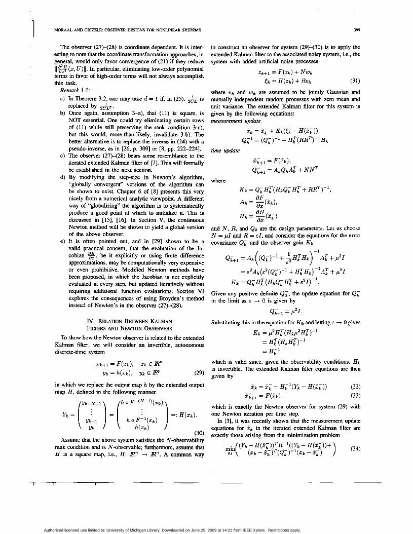
Fig. 1.

when u l ( t ) = 0.3 and uz( t ) = 0.0067.

Discrete-Newton observer: relative observer error e = ( e l , e2, e 3 ) , where e . - 7, z’-z’ for 2 = (0.2,0.02,0.005) and 2 = (0.02,0.2, 0.015)

I -

A discretization of the above system with sampling time T may then be expressed as

xk+l = FgL (xk) Y k = h(xk) (54)

and the state-to-measurement map is given by

. , Computing the rank of at a number of different points in the state space showed that the N-observability rank condition is indeed satisfied for N = 3. It was also found, however, that system (54) is poorly observable, indicated by ill-conditioning of z: ratio of its largest to smallest singular value for a sampling time of T = 1 (i.e., one hour) is on the order of 500. A typical response for the Newton observer is shown in Fig. 1, simulations showed however, that the Newton observer fails to converge if it is not initialized closely enough to the actual states, e.g., when

x = f : i 2 ) a n d ? = (0.2 ) . 0.02

0.005 0.015

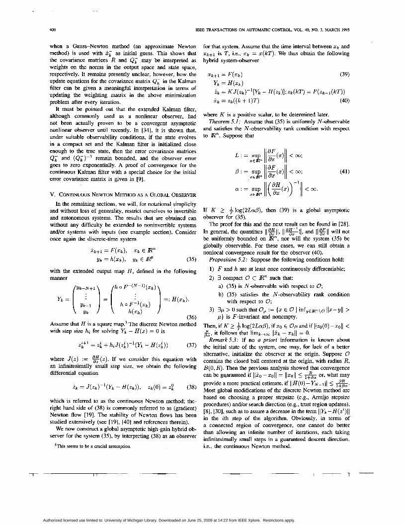
Given the time scale-sampling times in the order of minutes or even hours-there is virtually no restriction to available CPU time in the observer design. We therefore simulated the continuous Newton observer as well. It is given by

z k = F”k-2(Z,(kT)) pk = F”k-1

( z k ) -

As expected, this observer did converge for all physically feasible initial values. Responses are shown in Fig. 2 for four values of the observer gain K. The plot confirms our finding that the observer may fail to converge if K is too small.

- 6 ~ ~ ” ’ “ ’ ” ” ” ~ ’ ” ” 0 2 4 6 8 1 0

nme (in hours)

Fig. 2. is the relative observer error for z2, when u l ( t ) E 0.3 and u Z ( t )

Continuous Newton observer with different observer gains IC; shown 0.0067.

VIII. CONCLUDING REMARKS In this paper, we have provided a new observer design

method for nonlinear systems with discrete measurements. The method relies on asymptotically inverting the state-to- measurement map, which is constructed by relating the system’s state at a given time to a (predetermined) number of consecutive measurements. By using a continuous Newton method for the map inversion, the observer error was shown to converge to zero, globally and exponentially. If, instead, a computationally less expensive discrete Newton method is used, the observer shows quasilocal exponential convergence. Even more computational advantage may be gained by employing Broyden’s method, whose effect on the observer performance was also investigated. The theory was illustrated on an example. Results on using this observer in a closed-loop setting have been reported in [ 171.

ACKNOWLEDGMENT

The authors wish to thank A. TornamE for his insightful comments on the continuous Newton method.

REFERENCES

[ l ] D. Aeyels, “Generic observability of differentiable systems,” Siam. J . Contr. Optim., vol. 19, pp. 595-603, 1981.

[2] -, “On the number of samples necessary to achieve observability,” Syst. Contr. Lett., vol. 1, pp. 92-94, 1981.

[3] B. M. Bell and F. W. Cathey, “The iterated Kalman filter update as a Gauss-Newton method,” IEEE Trans. Automat. Contr., vol. 38, no. 2, pp. 294-298, 1993.

[4] W. M. Boothby, An Introduction to Differentiable Manifolds and Rie- mannian Geometry.

[5] S. T. Chung, “Digital aspects of nonlinear synthesis problems,” Ph.D. dissertation, University of Michigan, 1990.

[6] S.-T. Chung and J. W. Grizzle, “Observer error linearization for sampleddata systems,” Automatica, vol. 26, no. 6, pp. 997-1007, 1990.

[7] W. F. Denham and S. Pines, “Sequential estimation when measurement function nonlinearity is comparable to measurement error,” AIM., vol. 4, pp. 1071-1076, 1966.

[8] J. E. Dennis, Jr. and R. B. Schnabel, Numerical Methodsfor Uncon- strained Optimization and Nonlinear Equations. Englewood Cliffs, NJ: Prentice-Hall, 1983.

[9] F. Deza, E. Busvelle, J. P. Gauthier, and D. Rakotopara, “High gain estimation for nonlinear systems,” Syst. Contr. Lett., vol. 18, pp. 295-299, 1992.

[lo] J. M. Fitts, “On the observability of nonlinear systems with applications to nonlinear regression analysis,” Inform. Sci., vol. 4, pp. 129-156, 1972.

New York Academic, 1975.

-7- 1 1 ‘ I 1



[ l l ] B. A. Francis and T. T. Georgiou, “Stability theory for linear time- invariant plants with periodic digital controllers,” IEEE Trans. Automat. Contr., vol. 33, no. 9, pp. 820-832, Sept. 1988.

[12] J. P. Gauthicr, H. Hammouri, and S. Othman, “A simple observer for nonlinear systems; applications to bioreactors,” IEEE Trans. Automat. Contr., vol. 37, pp. 875-880, June 1992.

[I31 S. T. Glad, “Observability and nonlinear deadbeat observers,” in Proc. IEEE Conf Decis. Contr., San Antonio, TX, Dec. 1983, pp. 800-802.

[ 141 J. W. Grizzle and P. V. KokotoviC, “Feedback linearization of sampleddata systems,” IEEE Trans. Automat. Contr., vol. 33, pp. 857-859, Sep. 1988.

[I51 J. W. Grizzle and P. E. Moraal, “Observer based control of nonlinear discrete-time systems,” Univ. of Michigan at AM Arbor, Tech. Rep. CGR-39, College of Engineering, Control Group Reports, Feb. 1990.

[16] -, On Observers for Smooth Nonlinear Digital Systems (Lecture Notes in Control and Information Sciences), vol. 144. Berlin: Springer- Verlag, 1990, pp. 401-410.

[ 171 -, “Newton, observers and nonlinear discrete-time control,” in Proc. 29th CDC, Hawaii, 1990, pp. 760-767.

[18] K. A. Hoo and J. C. Kantor, “Global linearization and control of a mixed-culture bioreactor with competition and external inhibition,” Mathematical Biosciences, vol. 82, pp. 4342 , 1986.

[ 191 H. Th. Jongen, P. Jonker, and F. Twilt, Optimization in R n . Frankfurt am Main: Peter Lang Verlag, 1986.

[20] S. Karahan, “Higher order linear approximations to nonlinear systems,” Ph.D. dissertation, Mechanical Engineering, Univ. of Califomia, Davis, 1989.

[21] A. J. Krener, “Normal forms for linear and nonlinear systems,” in Differ- ential Geometry, the Interface between Pure and Applied Mathematics, M. Luksik, C. Martin and W. Shadwick, Eds, vol. 68. Providence, RI: American Mathematical Society, 1986, pp. 157-189.

[22] A. J. Krener and A. Isidori, “Linearization by output injection and nonlinear observers,” Syst. Contr. Lett., vol. 3, pp. 47-52, 1983.

[23] A. J. Krener, S. Karahan, M. Hubbard, and R. Frezza, “Higher order linear approximations to nonlinear control systems,’’ in Proc. IEEE Con$ Decis. Contr., LA, 1987, pp. 519-523.

[24] A. J. Krener and W. Respondek, “Nonlinear observer with linearizable error dynamics,” SIAMJ. Contr., vol. 47, pp. 1081-1100, 1988.

[25] D. G. Luenberger, “Observers for multivariable systems,” IEEE Trans. Automat. Contr., vol. AC-11, pp. 190-197, 1966.

[26] D. G. Luenberger, Optimization by Vector Space Methods. New York: Wiley, 1969.

[27] H. Michalska and D. Q. Mayne, “Moving horizon observers and observer based control,” preprint, 1993.

[28] P. E. Moraal and J. W. Grizzle, “Nonlinear discrete-time observers using Newton’s and Broyden’s method,” in Proc. ACC, Chicago, 1992, pp. 30863090.

[29] P. E. Moraal, J. W. Grizzle, and J. A. Cook, “An observer design for single-sensor individual cylinder pressure control,” to be presented at CDC, San Antonio, 1993.

[30] K. T. Murty, Linear Complementarity, Linear and Nonlinear Program- ming. Berlin: Heldermann Verlag, 1988.

[31] S. Nicosia, A. Tomambe, and P. Valigi, “Use of observers for nonlinear map inversion,” Syst. Contr. Lett., vol. 16, pp. 447-455, 1991.

[32] H. Nijmeijer, “Observability of autonomous discrete-time nonlinear systems: a geometric approach,” Int. J . Contr., vol. 36, pp. 867-874, 1982.

[33] K. R. Shouse and D. G. Taylor, “Discrete-time observers for singularly perturbed continuous-time systems,” to appear in IEEE Trans. Automat. Contr., 1993.

[34] Y. Song and J. W. Grizzle, “The extended Kalman filter as a local asymptotic observer for nonlinear discrete-time systems,” in Proc. I992 ACC, Chicago, 1992, pp. 3365-3369.

[35] E. D. Sontag, “A concept of local observability,” Syst. Contr. Lett., vol. 5 , pp. 41-47, 1984.

[36] A. TomamM, “An asymptotic observer for solving the inverse kinematics problem,” in Proc. Amer. Contr. Con$, San Diego, May 1990, pp. 1 7 7 4 1779.

[37] J. Tsinias, “Further results on the observer design problem,” Syst. Contr. Lett., vol. 14, pp. 411-418, 1990.

[38] A. J. van der Schaft, “On nonlinear observers,” IEEE Trans. Automat. Contr., vol. 30, no. 12, pp. 12541256, Dec. 1985.

[39] B. L. Walcott, M. J. Corless, and S. H. Zak, “Comparative study of nonlinear state-observation techniques,” Int. J . Contr., vol. 45, no. 6, pp. 2109-2132, 1987.

[40] P. J. Zufiria and R. S. Guttalu, “On an application of dynamical system theory to determine all the zeroes of a vector function,” J . Math. Analysis and Applic., 152, pp. 269-295, 1990.

Paul E. Moraal was bom in Drachten, The Nether- lands, in 1965. He received the engineering degree in applied mathematics from Twente University, Enschede, The Netherlands in 1990 and the Ph.D. degree in electrical engineering, systems, from the University of Michigan, AM Arbor, in 1994.

Dr. Moraal is currently an Engineering Specialist at Ford Motor Company’s Research Laboratory in Dearbom, MI. His current research interests include nonlinear control theory and applications of modem control theory to automotive powertrain control.

Jessy W. Grizzle (S’79-M’83-SM’90) received the Ph.D. in electncal engineenng from the University of Texas at Austin in 1983.

In 1984, he was at the Laboratoire des Signaux et Systkmes, Gif-sur-Yvette, France, as a PostDoc. From January, 1984 to August, 1987, he was an Assistant Professor in the Department of Electncal Engineering at the University of Illinois at Urbana- Champaign. Since September 1987, he has been with the Department of Electncal and Computer Science at the University of Michigan Ann Arbor,

where he is currently a Professor. He has held visiting appointments at the Dipartimento di Informatica e Sistemistica at the University of Rome and the Laboratoire des Signaux et Systkmes, SUPELEC, CNRSESE, Gif-sur-Yvette, France. He has served as a consultant on engine control systems to Ford Motor Company for seven years. His research interests include nonlinear system theory, geometnc methods, multirate digital systems, automotive applications, and electronics manufacturing.

Dr. Gnzzle was a Fulbnght Grant awardee and a NATO Postdoctoral Fellow from January-December 1984. He received a Presidential Young Investigator Award in 1987 and the Henry Russel Award in 1993. In 1992 he received a Best Paper Award with K. L. Dobbins and J. A Cook from the IEEE VEHICULAR TECHNOLOGY SOCIETY. In 1993, he received a College of Engineenng teaching award. He was Past Associate Editor of TRANSACTIONS ON AUTOMATIC CONTROL and system & Control Letters


40, 195’5 observer design for nonlinear systems with...

Documents