ieee vol. no. december functional expansions …web.eecs.umich.edu/~grizzle/gilbertfest/(36).pdf ·...

IEEE TRAMACTIONS ON ALTOMATIC CONIROL, VOL. AC-22. NO. 6, DECEMBER 1977 909

Functional Expansions for the Response Nonlinear Differential Systems

ELMER G.

Abstmct-This paper is concerned with representing the response of nonlinear differential systems by fnnctional expansions. An abstract theory of variational expansions, similar to that of L. M. Graves (1927), is developed. It leads directly to concrete expressions (multilioear integral operators) for the funaionals of the expansions and sets conditions on the differential systems which insure that the expansions give reasonable approximations of the response. Similarly, it is shown that the theory of analytic functions in Banach spaces leads directly to conditions which imply uniform convergence of functional series. The main results on differential systems are summarized in a set of theorems. some of which overlap and extend the recent results of Brockett on Volterra series representations for the response of linear analytic differential systems. Other theorem apply to more general nonlinear differential systems. They proride a rigorous foundation for a large body of previous research on Volterra series expansions. Tbe multilinear integral operators are obtained from systems of differential equations wKch characterize exactly the variations. These equations are of much lower order than those obtained by the technique of Carleman. A nonlinear feedback system selyes as an example of an application of the theory.

I . INTRODUCTION

HE USE of functional expansions to represent the Tresponse of dynamic systems is a well-established con- cept, dating back to 1942 when &. Wiener characterized the response of a nonlinear device by a Volterra series. Since then functional expansions (usually Volterra series) have played an important role in the modeling of nonlinear systems, both when the underlying system equations are known and when the system is characterized only by the availability of input-output data. This paper is concerned with the former situation. The dynamic system is described by a system of nonlinear differential equations and the objective is to obtain a local approximation of the system output by a functional expansion operating on the input. Usually, although not always, the expansion is a truncated power series.

There is a sizeable literature of prior research in this direction. In the 1950’s and 1960’s, Volterra series were derived and exploited in a variety of situations. Refer- ences [3]. [4], [ IO], [ 1 11. [ 181, [2 1E[23], and [26] give a good, although by no means complete, perspective of this work and include additional references to the literature. The main concern was with relatively simple, stationary dif-

recommended by G. L. Blankenship, Past Chairman of the Stability. Manuscript received August 25. 1976: revised August 17. 1977. Paper

Nonlinear, and Distributed Systems Committee. This work was s u p ported in part by the Air Force Office of Scientific Research, Air Force Systems Command, US.4F. under Grant AFOSR-77-3 158.

The author is Nith the Department of Aerospace Engineering and the

of Michigan, Ann Arbor. MI 48104. Program in Computer, Information. and Control Engineering. University

GILBERT

Qf

ferential systems. Multidimensional Laplace (or Fourier) transforms appeared frequently in both system characterization and response evaluation. For the most part, little attention was given to the validity of the Volterra series other than to assume without justification its uniform convergence. In this respect the paper by Bruni, DiPillo, and Koch [7] was a marked advance. For a general bilinear differential system it showed that the input-output map was a uniformly convergent Volterra series. By a technique due to Carleman, Krener [I71 has shown that a rather general class of nonlinear differential systems can be approximated by bilinear differential systems. This provides a path for extending, in a variety of ways, the results in [7] to general nonlinear systems. An example is the recent paper [ 5 ] by Brockett on “linear analytic” systems.

A different approach to a general theory is pursued here and in [ 121. The differential system is viewed abstractly as a mapping P from a Banach space of inputs into a Banach space of outputs. Then P is expanded in an appropriate abstract series and the series is interpreted concretely to obtain the desired functional expansion. Balakrishnan [2, sect. 3.61 takes a similar point of view in considering a bilinear differential system, although the details of his analysis are quite different from those which follow.

The most obvious candidate for the abstract series is a Frechet power series. The precise details may be found in [9] and, stated briefly, are as follows. Let P“’(uo)[ MI,][ w2]. . 1 [ w,] denote the ith Frechet differential of P at co with increments x*,:. . . ,”;. If P is k times continuously differentiable in a neighborhood of co,

P ( c o + c ) = P ( c o )

k l i = I 1 .

+ ~ P ” ’ ( c o ) [ u ] [ c ] . . . [ c ]+R, (c ) (1.1)

where IIRk(c)II < cjlcllk if Ilull< a(€). While (1.1) is appeal- ing and establishes connections with current research in polynomic systems theory (see [24] for a review), it is not obvious that the differentials exist and are continuous or that they can be determined easily from the description of the differential system. At least part of the reason for this difficulty is that P (’)(c0)[ H ~ , ] [ w ~ ] . . . [ vc,] contains much more information than is needed, since in ( 1 . I) , w,, , w, are all set equal to c. The “essential information” is contained in the ith variation of P at co. which is defined by

Authorized licensed use limited to: University of Michigan Library. Downloaded on February 2, 2010 at 15:47 from IEEE Xplore. Restrictions apply.

910 IEEE TRANSACnONS ON AUTOMATIC C O N l R O l V O L AC-22, NO. 6, DECEhiBER 1977

&;PC, (e ) = ( - g ) j P ( O , + at?) . ( 1-21 L O

In particular, k

P(oO+U)=P(C,)+ ,&'Pcn(~)+Rk(c) . 1 (1.3)

Because S'PCn(c) is obtained by examining P on a one-di- mensional subspace, it can be determined for differential systems by examining the solution of a differential equation with a parameter. As will be seen, this leads im- mediately to concrete characterizations of 6'Pc.(c) and to conditions on the differential systems which assure that IJRk(u)ll is bounded in a reasonable fashion. The expansion (1.3) was first considered by Graves [ 141 in 1927 and seems to have been neglected in recent years, except as it pertains to the theory of analytic functions in complex Banach spaces [ 151.

The plan and content of the paper are now summarized. In Section I1 the 'theory of (1.3) is developed for fixed k. It is pointed out that (1.3) is a sum of homogeneous functions and not necessarily powers of c. Conditions are given which guarantee that 1 1 Rk(c)il < ~ I 1 t ' l l ~ when lloll <&(E) or IIRk(c)II <pllcllkf' when llcll < p. Complete proofs are given because they are simple and informative and take little more space than proofs based on the results of Graves [14]. The theory of analytic functions in complex Banach spaces is reviewed in Section 111. The results are taken directly from Hille and Phillips [ 151 and lead to simple conditions which imply uniform convergence of (1.3) as k-+cc. In Section IV the methods of Sections I1 and I11 are applied to the differential system:

; = I *

x(t)=f(x(t),t)+U(t)g(x(t),t), x @ ) = < (1.4)

y ( t ) = h ( x ( W (1.5)

Here, x(t)E%.", c( t )E%., y ( f ) E % , and t E [ O , T ] . The terms in (1.3) are given exactly by the solution of differential equations whose order is much lower than those arising from the technique of Carleman. These differential equations lead directly to the characterization of (1.3) as a truncated Volterra series. Precise conditions on f,g,h which assure the validity of (1.3) are given in Theorems 4.1-4.4. Brockett's result [5] , [6] on the uniform convergence of the Volterra series is included. Similar results are obtained in Section V for the more general differential system:

~ ( t ) = f ( x ( t ) , u ( t ) , t ) , x ( O ) = t (1.6)

y ( O = h ( x ( t ) , N J ) (1.7)

where x(t)E%.", u ( t ) ~ C P ' , y ( t ) ~ 9 ' , and tE[O,T] . Here t' is the pair (u(-) ,<), so that the functional expansion for y ( t ) includes the effect of changes in the initial condition.

The derivation of the variational equations is usually much simplified whenf and h have a specific form. This is illustrated in Section VI by the analysis of a nonlinear control system. A discussion of the results and other applications of the approach is contained in Section VII.

The reader who is interested mainly in the application of the basic theory of (1.4)-(1.7) may jump to Section IV without loss of continuity. Sections I1 and I11 are of general interest because they constitute a methodology by which other types of systems may be analyzed.

11. APPROXI~MATION BY A Svu OF HOMOGENEOUS FLNCTIONS

In what follows it is assumed that 3 denotes the real numbers, T and % are real Banach spaces. 9l is an open set in q y , and P is a function from into >X.

The objective is to obtain a representation for P of the form

k

P ( C o + C ) = P ( C , ) + 2 Q ; ( C ) + R k ( C ) , G E N ( p ) i = I

(2.1)

N ( p ) = { t ' : llcll<p, cE'?], (2.2)

where p > 0,

and for i = 1,. . , k. Q, : 'T-+% is homogeneous of degree i, that is, for all c EL?^ and a E CG, Q,(ac)= a'Q,(c). Gen- erally, Rk(c) is to be small in some reasonable way, e.g.,

Before proceeding, it should be emphasized that (2.1) is not a natural generalization of Taylor's formula. This is because P (eO) +E:= Q, ( c ) is not necessarily a polynomial in t'.

Definition 2.1: The function Q, : Y-+%i is an i-power if there exist functions c, : '-$ 2+?lr,j=0,. . . ,i, such that for all c.5Erf and a .b€$ ,

IIRk(U)ll <Pllcllk+l.

i

Q , ( a ~ + f l Z ) = 2 cj(c,C)ai-'@. (2.3)

The function Qo + Zt=, Q, (G), Q, E Tli. is a polynomial of degree k if for i = 1; . . , k , Q, is an i-power.

E-xample 2.2: Let P(c)= r2f(f?) where ?-= g2, 3d = 9,. and r and 6 are polar coordinates in the plane. Clearly, P is homogeneous of degree 2. However, i t is a 2-power if and only if it is a quadratic form, i.e., there are real numbers aI.a2.a, such thatf(~)=a,cos'6+a2cos8sinB+ uj sin'f?. Thus. for k 2 and cO= 0, P = rZcos46 can be represented by (2.1), but the sum is not a polynomial.

I t is necessary to consider derivatives of continuous functions f: $3 +V. The notation (d/da)f(a.)=g(cY) means g( a ) E ?[? satisfies

j = O

lim I I g ( a ) - p - ' ( f ( a + P ) - f ( a ) ) l / = O . (2.4) P+O

I f f is defined on a closed interval of 9 and a is an end point. the appropriate one-sided limit is used. Higher


GILBERT: FUhXTlONAL EXPANSIONS FOR NONLINEAR DIFFEFENTIAL SYSTEhls 91 1

order derivatives are formed in the obvious way. For is defined for all u E N ( ~ ( E ) ) and a E[O, 11, and r(u, 1)= example, (d /da)2 f (a)=h(a) where h(a )=(d /da)g (a ) . &(I;). Moreover, for all I ; E N ( ~ ( E ) ) , ~ E [ O , 11, i= 1,. . . ,k, Only the simplest results from the theory of integration the function PLo+uc.e( p ) is continuous for I PI sufficiently are needed. I f f : %.+% has a continuous derivative g on small. Since P&(a+p)= P;o+ac;v(/?), this implies that [O,a], then the Riemann integral [14], [15] of g exists and the functions J~g(u )du=f (a ) - f (O) . Moreover, if y : %.+% is integra-

Definition 2.3: For CE ?X and u E T adopt the nota- ble and II g(a>ll< Y(ah then I l f ( 4 - f ( O ) l l < J:Y(4 &.

tion P;" ( a ) = P ( C + a.)

For all I; E ?- assume that there is an open interval, (- p(U, u), p(t; I;)) c CR, such that Pk; is continuous on the interval for i=O; . + , k. Then P is said to have a smooth kth variation at E and for i = 1;. . ,k, 6'P,: 'J'+%, which is given by

k

=P&&)- x ~ PLo;" (0)a'-* '=2 (i-2)!

S iPG(c )=($) 'P ( i7+a~) =P&(O), (2.6) r (u ,a )=P; ;c ( a ) - P& (0) (2.12)

is called the ith variation of P at E. Some observations are in order. Simple examples where

V = CR2 and % = 9. show that the continuity of P?,(a) in a does not imply the continuity of 6kP,(o) in either L; or 1;. The terminology "smooth" kth variation is an attempt to distinguish this difference. Since (d/da)'P(E+ apv) = Pi(d/d(ap)) 'P(U+ @I;), it follows that

C'

6'P, ( P C ) = piSiP, (I;), t 'E T-, ,8 E 9. (2.7)

Thus, SiPL0 is homogeneous of degree i and (1.3) meets the requirements of (2.1). Finally, when P has a smooth kth variation at 5+ ac, the identity (d/da)'P(G+ ac) = (d/dp)'P(t-+ ac + pc)lp=o implies

6'P,+u1:(u)=P$c(a), u E q C , O < i < k . (2.8)

The first approximation theorem can now be stated, Theorem 2.4: Suppose that there exists a po>O such

that {so} + N k0) c LX and P has a smooth kth variation at C for all C E { eo} + N(po). For all E > O assume that there exists a 6 ( E ) , 0 < 6 ( E ) <po such that the following condition is satisfied:

are defined and continuous in a for t ' E N ( 6 ( E ) ) and aE[O, I]. By (2.8) and (2.9), Ilrk(~,a)II < ~ I J c l l ~ . By the right side of (2.12), r,- ,(c,O) =O. Thus, integration of rk(u,a) with respect to a gives

~ ~ r k - l ( u ~ a ) ~ ~ = ~ ~ r k - l ( ~ , a ) - r k - l ( ~ , o ) ~ ~

< ~ a I ~ r k ( u , u ) l l d u < a ~ ( l u l l ~ . (2.13)

Repeated integration (noting that ri(c, 0) =0, i = 1,. . . , k-2, and r(c,O)=O) gives Ilr(c,a)ll <(ak/k!)~l l l ; l lk . Set- ting a = 1 completes the proof.

Theorem 2.5: Suppose that there exists a po > O such that { c0} + N (po) c 9t and P has a smooth ( k + 1)th variation at G for all E E { uo} + N(po). Assume that there exists an M > 0 and a p, O< p < po such that the following condition is satisfied:

I I ~ k + l P c o + a c ( C ) I I < M I I C l l k + l ,

for alluEN(p), a € [ O , 11. (2.14)

Then Rk (u) in (1.3) satisfies

for all . E N ( G ( E ) ) , a € [ O , 11. (2.9) Prooj Proceed as in the previous proof with 6 ( ~ )

Then for any E > 0, Rk(c) in (1.3) satisfies replaced by p and add to (2.12) the function

Proof: Choose E >O. Then which is continuous in a for a E[O, I]. Using rk(u,O) = O k and the bound (2.14) gives, by integration, IIrk(c,a)II <

r(G,a)=P(uo+a.)-P(t'o)- 2 ;s'P,,(ao) Ma 1 1 1 ; I J k + ' . Repeated integration, as before, completes the l = l 1 .

k 1 l = i 1 . by Graves [14] in 1927. In his Theorem 5, '7; is a linear

proof. = p - p - x --pio; , ( o ) ~ ; (2.1 1) These theorems are in the spirit of the results obtained


metric space, is a complete linear metric space, and &(e;) is an integral. Notice that the completeness of 5- has not been used in the above proof. The normed spaces have the advantage that they permit the main conditions. (2.9) and (2.14), and the error bounds, (2.10) and (2.15), to be expressed in particularly useful ways.

Remark 2.6: Consider the conditions

IlskP,(0)-skPtio(o)ll<€llcllk,

f o r a l l u E ~ , I : E { o , } + R r ( G ( ~ ) ) (2.17)

and

~lS"+"~,(c)l l < ~ l l u l l ~ + ' , for all LIE?-, ~ ~ { c , } +,V(p).

(2.18)

Because of the homogeneity of SkPc and Gk+ 'PC, these conditions imply, respectively, conditions (2.9) and (2.14). In many applications of Theorems 2.4 and 2.5. these conditions are easier to work with and can be verified. Example 2.2 shows that (2.9) and (2.14) can be satisfied when (2.17) and (2.18) cannot.

It is of interest to know whether or not the expansions

established and a suitable account appears in Hille and Phillips [ 151. In this section several key results from [ 151 are stated in the notation of Section 11. Although [15] encompasses a much richer theory, what is used here seems sufficient for many applications. It leads to easily verified conditions which ensure the uniform convergence of (1.3) for k 4 m . As a bonus, these conditions imply that (1.3) is a power series, i.e., for all i 2 1, G'PL', is an i-power.

In this section it is understood that '3 is replaced by the complex field 2, and that 'I' and ?l.f are complex Banach spaces. The notation (dldol) f ( a ) = g ( a ) means (2.4) holds for all complex /3-0. Otherwise, the notation is the same as in the previous section.

Definition 3.1 (Definition 3.17.2 of[l5]): Let %.cy be an open set. The function P : %+?LC is analytic in % if: 1) P has a first variation at all C E 3, i.e.,

( z ) P ( L + a e ) l d =S'P,(t:) a = O

exists for all EE TL and c E T-; and 2) P is locally bounded, i.e., for all <E 3 there is a p($ > 0 and a finite M(E)>O such that { C } + N ( p ( q ) c : T and

presented above are in some sense unique. A result of Graves [14], modified (proof omitted) to suit the present I I P ( c ) l l b M ( t . ) , forallcE{G}+N(p(C)). (3.2) situation, answers the question affirmatively.

Theorem 2.7: Let Qi : V+%, i = 1.. . . , k be homogeneous of degree i. Suppose P satisfies the hypotheses of Theorem 2.4. If for any E > 0 there exists a & ( E ) such that

Theorem 3.2 (Theorems 3.17.1 and 26.3.5 of [ 1 5 ] ) : Assume that P is analytic in the open set LX crf. Then a k P c : Y+qK exists for all positive integers k and DE%. Moreover, SkP, is a k-power.

k P(c,+c)- P(0,)- Qi(C) <&llcll".

i = I ll Theorem 3.3 (Theorem 3.17.1 of [15]): Let P satisfy the hypothesis of Theorem 3.2. Then for there exists a p>O, dependent on eo, such that

then

Q ~ ( C ) = T J S ' P ~ ~ ( C ) , 1 i = l , * . . , k . (2.20) (3.3) That is, given any E >0, there exists a positive integer k(E)

Suppose P satisfies the hypothesis of Theorem 2.5. If there such that Rk(e) in (1.3) satisfies exist k > O and F , O < F < p , , such that

k IIRk(c)ll<e forallk>k(E),cEN(p). (3.4) P ( o , + u ) - P ( u , ) - (Icllk+'?

i = I

for all c E N ( p ) , (2.21) IV. THE DIFFERENTIAL SYSTEM (1.4)-(1.5)

then (2.20) holds. In specific applications of the preceding theory it may

be important to determine that P ( uo) + I ( 1 /i!)SiPz0(c) is a polynomial of degree k. Often, as is the case in Sections IV, V, and VI, this can be done by simply inspecting the concrete forms of SiPc,(c) for i = 1;. . , k .

111. POWER SERIES

It is possible to extend the above ideas to infinite series. The most natural framework for doing this is the theory of analytic functions in Banach spaces. This theory is well

Functional expansions for both x ( t ) and y ( t ) will be obtained. To distinguish between the two corresponding mappings of e, the notations

x ( t ) = P ( G ) ( ~ ) (4-1)

are adopted. Before considering the expansions for P and p , some additional notations and assumptions are needed.

Let c"([O,T],W) be the (Banach) space of continuous functions from [0, TI into W with norm llell =


GILBERT: FUNCTIONAL EXPANSIONS FOR NONLINEAR DIFFEREhW SYSTEMS 913

suplO,,je(t)) where le(t)l is the sup norm of e ( t ) over the where, for simplicity, arguments have been omitted, and it components of e(t). It is assumed in (1.4) that G E T = is understood that g and the derivatives of f and g are e([O, TI, CR). The notation f , g ,h E C,'k) is used when evaluated at ( z ( t ,a ) , t ) where z( t ,a) is the solution of (4.4). f,g : 9" X [0, T]+W and h : 3" X [0, TI+-% are continu- Define ous and have continuous partial derivatives of order k with respect to the components of x in %" x[O, TI. It is X ( t ) = P ( z ; ) ( t ) , x i ( t )=S iPC( l ; ) ( t ) . (4.6) assumed that f , g ,h E C,") with k 2- 1. Let 3 = E ( [ O , TI, '%) and '?X = e([O, TI, '3"). For P, % plays the role of %- in Sections I1 and 111: forp, 9 plays the role of %.

Differential equations for the variations of P are obtained from ~ , ( t )=z~( t ,O) . For example, (4.4) and (4.5) yield

In general, P and p are not defined on Y because the solutions of (1.4) may have finite escape time. This question is treated in the Appendix, Theorem A. 1 and Remark A.2, and it is shown that if (1.4) has a solution on [0, TI for l; = u, E T, then there is a neighborhood of q,, 9 t , such that P : %-+>X and p : +% . Thus, for such co it is possible to proceed according to the plan of Section 11. To clarify the presentation, the characterizations for 6'P, and

are derived initially without full justification. Then, the conditions required in Theorems 2.4. 2.5, and 3.3 are verified rigorously. The results concerning the functional expansions for P and p are summarized in a set of theorems.

Derivatives of f ,g ,h with respect to x appear in the development and it is necessary to have a compact way of denoting them. If j E C,'", then f has a kth Frechet differential with respect to x [9]. This differential has k increments, wI, * . . , wk E C R n $ and is written f 'k)(~,t)[wI]- * . [ w k ] . This is a compact notation because each of the n components of f(,) is a linear combination of products of k numbers, where in each product the numbers are taken from (one from each) the components of w,, . . , w k . The differential is symmetric (the ordering of w,; . . ,wk is immaterial) and k-linear (linear in each %vi taken separately) [9]. For brevity, the designation (x,t), which indicates where the differential is evaluated, will be omitted if it does not cause confusion. When f',) has repeated arguments, a power-llke notation is used, e.g., f'4'[ wI I[ w3][ w2][ w I ] =j'4)[ wIl2[ w2][ w3]. Because of the symmetry, this is only a slight abuse of notation. The same notation and remarks apply to g and h.

Let C E 9 Z . and G E Y. To obtain the characterization of 6'P,-(v), define

~ ( t , a ) = P ( r ; + a c ) ( r ) , t , ( t :a )= - P(t?+at')(t). ( a i

(4.3)

It is clear that t ( t : a ) is given by the solution of

i = f ( ~ , t ) + o ( t ) g ( _ 7 , t ) + ( ~ ~ ( r ) g ( ~ , r ) , ~ ( 0 , 0 1 ) = ~ . (4.4)

i = f ( x , t ) + a ( t ) g ( x , t ) , X(O)=<

~ l = A ( X , t ) x l + r : ( t ) B ( x , t ) , x,(O)=O

~ 2 = A ( x , t ) x 2 + A ~ . l ( ~ , t ) [ x l ] 2

+ u ( t ) { B : ( x , t ) [ x , ] } , x2(0)=0 (4.7)

where A(~,t)xl=f~')(~,t)[xl]+~(r)g~l~(X,t)[xl], B ( x , t ) =

and B:(x, t)[xl] =2g(')(Z, r ) [x , ] . Continuing in a similar fashion and omitting the arguments Z, t gives

g ( x , t ) , A;,,(?, t)[x1l2 = f ( 2 ) ( ~ , t)[x,12 + ~ ( t ) g ( ~ ) ( ~ , t)[xll2,

. . . .

A few comments concerning these equations may be useful. The equation for x, is the usual linearization of (1.4) about the reference pair T(t) , z\(t). For x k , k > 1, the equations have (the same) linear dynamics, but with forcing terms Fk and oCk. Fk is a sum of j-linear, symmetric functions of the type ._., $[ x,,]. . * [ x i / ] . The in- d ices i , ; . . , i , sa t i s fyO<i ,S i , . . . < i jandi ,+ i ,+- . -+ i j = k . The last result follows because x, must be a homogeneous function of degree k in u [see (2.7)]. Similar remarks apply to the term G k and the functions

__.. ,;[x,,]--.[x,] except i , + i , + - - . + $ = k - ~ . It is clear that the complexity of Fk and G k mounts rapidly with k.

Differentiation of this equation with respect to (Y yields B~ noting that differential equations for the I,([,.). For example, if j ( z , r ) = f ( z , t ) + f i ( t ) g ( z , t) , p ( f i+aG)( t )=h(Z( t ,a )J) (4.9)

i,=J~"[zl]+avg~~~[zl]+Gg,tl(o,a)=o and proceeding similarly, equations for the variations

i2=J(')[ t2] +a@)[ t2] + p [ z1]2+avg(2)[ z1]2 Yi(t> = h ( u ) t d (4. IO)

+ 2 v g ( " [ r , ] , z 2 ( 0 , ~ ) = 0 (4.5) can be derived. For i = 1,2,


914 IEEE TRANSACTIONS ON A~TOMATTC C O ~ O L , VOL. AC-22, NO. 6, DECEMBER 1977

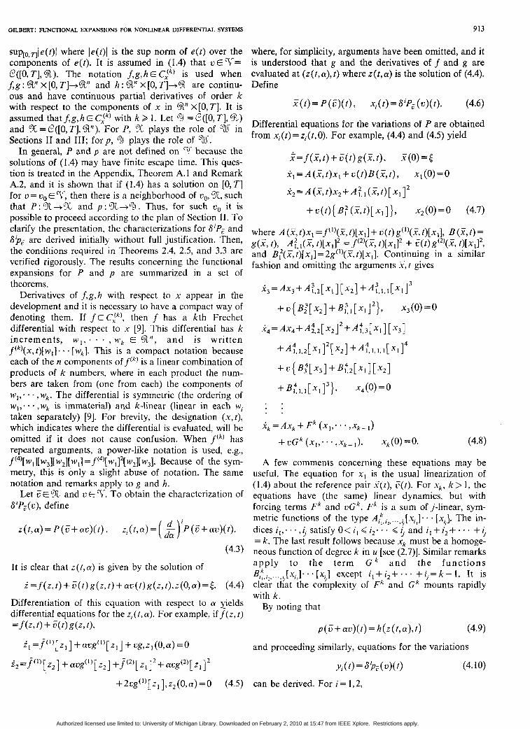
" wik where i,, * ,ik is any permutation of the integers 1,2; . * , k . In Fig. 1 this notation helps to sort out those "parts" of (4.7)-(4.8) and (4.11)-(4.12) which are linear (the L;) and those which are nonlinear (the Mi).

'I Because of the special structure of (4.7)-(4.8) and (4.1 1)-(4.12), it is easy to integrate successively the equa- .'

,~ illustrate, consider the equations .(4.7). Let % ( t ) be the fundamental matrix defined by % = A ( X ( t ) , t)$, s(0) = I . Then the variation of the parameters formula gives

.~ . . ~ ~ ~ ~ ~ . . . ~ ~ ~ ~ ~ ~ ~ . ~~~~ .... ~~~~ .... ~ tions to obtain integral formulas for 6'P, and 6'P,(u). To ' , X %

.... ~.. .~~ ..... ~.._._

I _ .

6 ' P ; ( c ) ( t ) = x , ( t ) = / Wi (t,a)r;(a)da (4.14) T

0

'Y3

Fig. 1. Structural representation of the variational equations for the w,'(t7a)=%(t)5-'(a)B(x(u),a), O < o < t < T system (1.4)-(1.5). =0, 0 < t < u < T. (4.15)

. y , = C ( F , r ) x , Using this result to express x l ( t ) in the last equation of (4.7) yields . , -

y 2 = C ( Z f ) X 2 + c;, (X,t)[x,]2 (4.11) T i - 8 2 P G ( e ) ( t ) = X 2 ( t ) = j J w,'(t,al,a2)c(o,)c(u,)du,da,

where C(X, t j x , = h(')(F, [ ) [ x l ] and C:,(X, t)[x,12 = 0 0 hC2)(X, t)[xl12. For i = 3,4,. . . , k, (4.16)

where

. . (4.12)

where H k is a sum ofj-linear, symmetric functions of the =0, O<t<o,< T or O < f < a 2 < T. (4.17) type Cl,12, . . . , i , [xi , ] . [ X $ ] where the indices i,!. . ,$ satisfy 0 < i , < 1 , . . - < i j a n d i , + i , + . - . + i j = k . Although the formulas become even more complex, it is

Equations (4.6)-(4.8) and (4.10)-(4.12) characterize the clear that the process can be continued for i >2. Thus, variation of P and p . As indicated in Fig. 1, these equa- there are functions W ~ ( t , o , ; . . ,a,) such that

tions have a special structure involving a patterned inter- T T

connection of vector multipliers M j and linear dynamic X;(t)=6'pc(c)(r)= J * . * / wi (f3al,* * . ,aj) systems L;. In this representation L is the linear map of elements e E 5% into elements w E % which is defined by -u(u,)- * * c(u;)~u,. * * d ~ ; . (4.18)

0 0

Similarly, +=A(X,t)w+e(t) , w(O)=O. (4.13)

T T .

The notation w, X w2 indicates a vector whose components are all possible products of components of w , times com- .~(U,)....(U;)~U~...~U; (4.19) ponents of w2 with a systematic scheme of ordering. Thus, if w , has dimension n, and w2 has dimension n2, kt', X w 2 where has dimension n,n2. Similarly, w , X w2 X w3 = ( w , X w 2 ) X w3, w2 = w x w, and so on. Using this notation a symmet- wi(r ,a)= ~ ( , ( t ) , t ) ~ d ( t , a ) (4.20) ric, k-linear form D [ w l ] [ w 2 ] . . . [wk] can be written DM], X w2 X . . . X w, where D is interpreted as a linear mapping. and

y j ( t )=8ba(c) (r )=J S, w;(t,a,,.~-,uj) 0

the property that Dw, X w2 X * - X w k = Dw;, X w j 2 X . X t- C:l ( X ( t ) , f ) [ W; ( t , a , ) ] [ Wi ((,a2)]. (4.21)


GILBERT: FLh'CTIONAL EXPAUSIONS FOR NONLIhTAR DIFFEREhTIAL SYSTEhiS 915

Substituting these characterizations for S'PJc) and into (1.3) gives concrete expansions for x ( t ) and y ( t ) .

Let xo(t) and y,(t) be given, respectively, by (1.4) and (1.5) with c(t)= Go(t). Then setting E ( t ) = co(t) in (4.7), (4.Q (4.1 l), and (4.12) yields

x ( t ) = x 0 ( t ) + 2 k 1 ~ X , ( t ) + R , ( t ' ) ( t ) (4.22) ; = I .

k 1 ~ ( t > = ~ o ( t > + C i lY i ( t )+rk (G) ( t ) . (4.23)

i = l .

If the integral formulas (4.18) and (4.19) are used (with U= eo) in these equations, they become truncated Volterra series for x (t) and y ( r ) .

It remains to be shown that the preceding steps are justified and that the remainder terms in (4.22) and (4.23) are bounded in a suitable fashion. This will be done using standard tools from the theory of differential equations and Theorems 2.4, 2.5, and 3.3. The results are contained in the following theorems.

Theorem 4.1: Let j ,g , h E C:") and suppose (1.4) has a solution on [0, TI for e= eo E 'T. Then there exists an open set YL, eo E TL c Y: such that P and p are defined in 97- and have smooth kth variations in %. For i = 1, * , k and ~ € 3 , SiP,(c) and 61p,(c) are given by (4.6)-(4.8) and (4.10)-(4.12) or (4.18) and (4.19). The kernel functions W;(t ,u , ; . ,u,) and w ~ ( t , u , , * - ,ai) are calculated from (4.6)-(4.8) and (4.10)-(4.12) by the process described above and are continuous for all t , u l , . - ,a, E[O, TI except for t = a, or u, = 5, ij = 1, . , k where jump discontinui- ties may appear.

Proof: By Theorem A.l and Remark A.2 of the Ap- pendix, there exists a p > 0 such that P is defined in '?X = { uo} + N (p). Since for all 2. E T and c E 'IT, E + ac E % for IaJ sufficiently small, (4.4) has a solution for la/ sufficiently small. Moreover, if (4.4) is written as

-

i = F ( z , a , t ) , z(O)=$', (4.24)

it is clear that F is k times continuously differentiable in z and a. From this it is known (see [19, ch. 11, sect. 41) that z ( t ,a ) is k times continuody differentiable in a for a in a neighborhood of a = 0. This proves that P has a smooth kth variation at I5 for all CE%. Because of the differen- tiability of t, j , and g, the steps leading to (4.7) and (4.8) are valid. Thus, these differential equations define u'P,-(c> = xi for i = 1,. 1 , k . From (4.9), h E C,"), and the differen- tiability of z ( t , a ) with respect to a, it follows that p has a smooth variation in % and (4.10)-(4.12) are valid. Be- cause F(t) is continuous, all the terms in (4.7), (4.Q (4.1 l), and (4.12) are continuous in t. This justifies the use of the variation of parameters formula and shows that Wi and w; are continuous on the indicated subset of [0, TI'+'.

Theorem 4.2: Let f ,g ,h E C x k f 1 ) and suppose (1.4) has a solution on [0, TI for e= coE T,?. Then there exists a p > O and p > O such that

II&(c)II? I!r,(C)II<pLiICIIk+l (4.25)

for all cE'?'such that 1 1 0 1 1 <p. Proof: First, R,(u) is considered. Because of Theo-

rem 4.1 and Remark 2.6, it is clear that the hypotheses of Theorem 2.5 are satisfied if (2.18) is satisfied. From Re- mark A.3, X= P(5) satisfies llXll<Ko for G E { z ) ~ } + N ( ~ ) = 9. This means that there are constants Gl and f i 2

such that IA(F,t)x,l<@,Ix,I and IB(Y,t)l 9G2 for all t E [0, TI, E E 3. By the Gronwall inequality [ 191 it is known that if w satisfies (4.13), then l l w l l Q (TexpM,T)IIell. Combining the results of the preceding two sentences and applying them to the differential equation for x I shows that there exists an M , such that llx, 1 1 < M,IlulJ for all I5E % and c E Y. Using this result and similar reasoning, it can be seen from the differential equation for x2 that there exists an M, such that llx211 < M211c112. The process can be repeated until it is shown that there exists an A4 such that IIxk+,ll<MIIcllk+l for all I5E TL and G E YO, which implies that (2.18) is satisfied. Thus, the bound (2.15) follows from Theorem 2.5. In a similar way, (4.11) and (4.12) withllxill <M,llt:ll' show that there exist mi such that Ilyjll <millell'. Using the same argument and defining p ( k + l)! = max { M,+,, m,+ ,} completes the proof.

Theorem 4.3: Let f,g, h E CJk) and suppose that (1.4) has a solution on [0, TI for c = eo E T. Then for any E > 0, there exists a S ( c ) such that

llRk (C)ll, Ilr,(u)ll <c l l c l l k (4.26)

for all e E Y such that lloll < a ( € ) . Proof: Because of Theorem 4.1 and Remark 2.6, it is

sufficient to show that P and p satisfy (2.17). Since the notation becomes very burdensome, this will be done only for P and k =2. From this it should be clear how the proof proceeds for p and k > 2. Define i i ( t ) = 8'PC(c)(t) - S'P,,(c>(r). Then it is clear from (4.7) that

~ , = A ( x o , t ) i l + ( A ( F , t ) - A ( ~ o , t ) ) ~ ~ l

+U(t ) (B(F, t ) -B(x0 , t ) ) , i , ( O ) = O . (4.27)

By Theorem A.1 it follows that ~ ~ F - x o ~ ~ < K ~ ~ C / ~ , C=U- eo. Using the continuity of j ( ' ) ( x , t ) and g(l)(x, t) , it is clear from this that there exists a f l ( ~ ) such that I(A(F,t)- A ( x , , t ) ) x , ( < ~ l x ~ l and Ic ( t ) (B(F , t ) -B(x , , t ) ) l<~ lo ( t ) l if

1 1 1 5 ) 1 < s(c). Applying the Gronwall bound of the previous proof and recalling that Ilx, / l<M,l lul l , it follows that there exists a SI(€) such that Ili,Il<cllcll if 11611<S1(c). Now consider the proof of (2.17). From (4.7) it follows that

i 2 = A ( x 0 , t ) ~ ~ + ( A ( X , t ) - A ( x , , ~ ) ) X 2 + A ~ , , ( X , t ) [ X 1 ] 2

- A : , ( x o , t ) [ x , - i , ] 2 + F ( t ) B : ( x : t ) [ x l ]

- c ( t ) ~ ~ ( x , , t ) [ x , - i , ] , ~^,(O)=O. (4.28)

Using the representation for multilinear forms which was introduced in the discussion of Fig. 1, this becomes


916 IEEE TRANSACTIONS ON AUTOMATIC COhTROL, VOL. AC-22, NO. 6, DECEMBER 1977

~ 2 = ~ ( ~ 0 , t ) ~ 2 + ( ~ ( ~ , t ) - ~ ( ~ 0 , t ) ) x 2 + ( ~ ~ , 1 ( ~ , t )

- A ?, (x,, I))$ + 2~ ?, (X,, O x , x 2,

-A:,,(x,,t)i:+o(t)(B:(x,t)

- B ~ ( x , , t ) ) x , + u ( t ) B ~ ( x , , t ) i , , 2,(0)=0. (4.29)

Because of the continuity of f 2 ) ( x , t ) and g(2)(x, t ) and the definitions of A & ( x , t ) and B:(x,t) , IIx211 < M2110112, llxIll <M,IIoll, and ~ ~ 2 , ~ ~ ~ c ~ ~ o ~ ~ f o r ~ ~ I ? ~ ~ < 8 , ( c ) , it can be argued that there exists a S2(c) such that 1151) < i 2 ( c ) implies that the sum of the last four terms on the right side of (4.29) are bounded in norm by ~ 1 1 0 1 1 ~ . This and the Gronwall bound establish the existence of a2(c) such that l l i 2 1 1 < ~ l l t ' 1 1 ~ if I l I ? l l =lIC-o,\l < S2(c) . The definition of i2 shows that (2.17) is satisfied for k = 2 .

Theorem 4.4: Assume that f ,g,h are analytic functions x, i.e., f , g , h E CJ') when the complex field 2 replaces 9. Suppose that (1.4) has a solution on [0, T ] for c = eo E ?#-. Then the variations S'P,,(c) and S$Jc) are defined by (4.6)-(4.8) and (4.10)-(4.12) or (4.18) and (4.19) for all i > O and (4.22), (4.23) converge uniformly in a neighborhood of s,, as k j m . Specifically, there exists a p > O such that the following statement is true: given any E > O there exists a positive integer k(E) such that

IlRk (c)ll, Ilr!f(u)II < E (4.30)

for all k 2 k(c) and o Eqf which satisfy lloll <p. Prooj In all of what follows 3. has been replaced by

e. As indicated in Remark A.4, this does not change the results of the Appendix. Thus, as before, (4.24) defines z( t ,a)=P(C+ao)( t ) for all G E { ~ , } + N ( ~ ) = % , e€?-, and a Et?, ]dl sufficiently small. Moreover, since F(z ,a , t ) is analytic in ( z , a ) for each t E[O, TI, it is known [ 19. ch. 11, sect. 51 that the solution is analytic in a. Thus condition I ) of Definition 3.1 is satisfied. Condition 2) follows because Remark A.3 implies that P is bounded on Yl. Hence, P is analytic in L%. Because of the analyticity of h and z( t ,a) , (4.9) shows that p(C+ao)(t) is analytic in a. The bound on P implies a bound on p and. hence, p is analytic in u%. The results of the theorem follow im- mediately from Theorems 3.2 and 3.3.

V. THE DIFFERENTIAL SYSTEM (1.6)-( 1.7)

tial derivatives of order k with respect to the components of x and u in CP' X qrn X [0, TI. It is assumed that f , h E C[tiJ with k > 1. If (1.6) has a solution on [0, TI for c0 E f, then Theorem A.1 of the Appendix implies the existence of an open set % c r< such that (1.6) has a solution for all 2; ET. Thus, the maps P: %+'X and p : %+9, where % = C([O, TI, CRn) and 9 = Q([O, TI, a'), are defined. The objective is to expand P andp in expressions of the form (4.22) and (4.23).

Mimicking the development of the previous section, z ( t , a ) and z j ( t , a ) are defined by (4.3). When CEUn., G E T and la1 is sufficiently small, z ( t , a) is defined and is the solution of

2=f ( z ,U( t )+a~( t ) , f ) , z (O .a )=$+a& (5.1)

If f E C$,i), z(r,a) is k times continuously differentiable with respect to a for a in a neighborhood of a = 0 [ 19, ch. 11. sect. 41. Thus, it is permissible to differentiate (5.1) k times with respect to a. Let f " ' ( x , u , t ) [ ( ~ ~ , I . t . . ~ ) ] . [(zj ,wj)] denote the ith Frechet differential of f with respect to (x, u ) with increments ( z , . w1), . , ( z i , x;) E an X am. Then noting that (d/da)'(z,G+cyu)=(ri .0) for i > 1, it is clear that

where it is understood that the differentials are evaluated at (z(t ,a),U(t)+ azl(t), t). Finally, from (4.6). x i ( t ) = zj(?,O), and the symmetry of the differentials, it follows that the (smooth, up to order k ) variations of P at C are given by

i=f (x ,u( t ) , t ) , x(o)=$ In this section functional expansions for the system ~ l = f i l ) ( ~ , u ( t ) , t ) [ ( ~ , : u ( t ) ) ] . x,(o)=<

(1.6)-( 1 . 7 ) are examined. Although there is an appreciable increase in the complexity of the notation, the schema of 1 , = f < ' ) ( x , u ( r ) , t ) [ ( x 2 , O ) ] the previous section applies with only minor modifica- tions. Because of this, the emphasis is on results, and + f " ) ( x , u ( t ) , t ) [ ( x , , ~ ( t ) ) ] ~ , -y2(0)=0, many details concerning formulas and proofs are omitted.

where now x( t ) is the solution of (1.6), y ( t ) is given by (1.7), and o is the pair (u ( * ) ,< ) . It is assumed that G E T = +3P2)(X,u(t),t)[(x2,o)][(x,,u(r))] C?([O,T],CRrn)xP and IIoII=IIuII+IEI. The notationf,hE C[li) is used when f : CRn X qrn x[O, and h : 9'' X ?Xrn X [0, TI+%' are continuous and have continuous par- (5.3)

As before, the notations (4.1) and (4.2) are adopted, a,=P1'(x,.(?>,t)[(x3.O)]

+ f 3 ) ( ~ , ~ ( t ) , t ) [ ( x l , ~ ( t ) ) I 3 , x3(0)=o


GILBERT: F'UXCTIONAL EXPANSIONS FOR NONLINEAR DIFFERENTIAL SYSTEMS 917

;&, ~. . -. . . . . . . . . . . . . . . . . . .. where A , B , C, and D are t-dependent matrices and the

" I I X , .") remaining terms are r-dependent bilinear (not necessarily L, ;

symmetric) functions. For i > 2, similar expressions can be l x I . U I ~ written, although the number of multilinear terms which

appear grows rapidly with i. When the variation of param- [+ol eters formula is applied to (5.6), it is seen that the varia-

tions can be written as follows: T

a l p , ( U ) ( t ) = X , ( t ) = / 0 w : ( t , u l ) [ u ( u , ) ] d u , + ~ ~ ( t ) [ 5 ]

(5.7) a'P, (u) ( t )=x , ( t )

Fig. 2. Structural representation of the variational equations for the system (1.6)-(1.7).

Observing that p ( 6 + av)( l ) = h ( z ( t , a ) , U(t ) + ~ ( t ) , t) , using the notation (4.10), and assuming that h E C,l".?, shows that the (smooth, up to order k ) variations of p 'are given by

y,=h( ' ) (x ,U(r) , t )[( .u , ,u(r))]

The variational equations have a special structure which is indicated in Fig. 2. As in Fig. 1, the multilinear forms are interpreted as- linear mappings of "product vectors." + ~ ~ , o ( t ) [ ~ I 2 + Q o 2 ; o ( t ) [ u ( t > ] [ q . (5.10) The figure shows that the system (5.3)-(5.4) is a intercon- nection of vector multipliers (Mi) and linear dynamic The functions labeled W,W,@,,Q utilize the notation which systems (I,;). The operator L, which maps elements (e,q) € has been established for linear and bilinear forms and are X X CRn into elements M, E Y , is defined by determined from the data in (5.6). For example,

helpful to write (5.3)-(5.4) in greater detail. For example, +2 t 5 ( r ) 5 - y u ) the equations for xi,y,, i = 1,2, are written I

A : , ( . r ( 4 > w , u ) [ w: ( % . I ) [ ~ l ] [ m ~ , [ t ] ] ~ ~ . i , = A x , + Bu, s I (0) =t 1 2 = A x 2 + A ~ . , [ ~ , ] 2 + B & [ u ] 2

0 < U l < t < T

=O, O < t < a , < T (5.1 1)

y , = Cx, + Du where 5(t) is the fundamental matrix corresponding to A . The multiplier 2 arises from the fact that A?., is symmet-

y2= Cx, + Ct [ x , ]'+ 0: , [ .I2+ D ; , [ u ] [ xI ] (5.6) ric; the required change in order of integration is permissi-

+ B : ; ; , [ u ] [ x , ] , ~ 2 ( 0 ) = 0


918 IEEE TRANSACTlOKS ON AUTOMATIC COSTROL, VOL. AC-22, KO. 6, DECEhiBER 1977

ble because the bilinearity of A ;. leads to the identity

[ w,’ ( a , o l ) [ u ( o l ) ] ] [ @ ~ ( ~ ) [ S ] ] ~ ~ l ~ ~ . (5.12)

It is easy to see that W:2 and w ! , ~ are zero for 0 Q t < u1 Q T or 0 Q c < u2 Q T, and are continuous in t ,al ,u2 except at t=u1,u2 or ul=u2; W,‘, W&, w;, w ~ f , ~ , w ~ , ~ , 2 and (5f;o are zero for 0 9 t < u1 < T, and continuous in t ,u, for 0 Q uI 9 t 9 T ; @A, @& w& +A, u ~ i , ~ , +i,o, and are continuous in t for 0 Q t Q T. Similar results hold for 2 < i < k, although the complexity of the formulas is for- midable.

Even when <=O, the above formulas do not lead to a truncated Volterra series. This is because of the terms corresponding to W:l, w;,~, wi, ~ ~ ~ , ~ ( t ) . If “impulsive” kernels or Stieltjes integrals are allowed, the terms may take on the appearance of terms in a Volterra series. For example, if < = O , 6$,(u)( t ) can be written

T T WW=/ 0 0 / W 2 ( t W 2 ) [ u<.J][ “ ( 0 2 ) ] 4 d U 2

(5.13)

where

W 2 ( ~ ~ ~ , , ~ 2 > [ ~ I ] [ ~ 2 ] = W : 2 ( t 7 ~ l ~ ~ 2 ) [ ~ 1 ] [ ~ 2 ]

+ s ( . , - ~ , > w ~ , , ( t , ~ l ) [ ~ I ] [ ~ 2 ]

+ ~ ( ~ - - l ) ~ ( t - - 2 > w ~ . o c ~ > [ u l ] [ ~ 2 ] (5.14)

and S ( I ) is the Dirac “function.” The preceding characterizations of P and p can be

substituted into (4.22), (4.23) to obtain functional expansions for P and p . The results are made precise in the following theorems, Proofs are omitted, since they are similar to those of the previous section and involve rather lengthy notations.

Theorem 5.1: Let f, h E C)!,)u, and suppose that (1.6) has a solution on [0, TI for TJ = ( u , 5) = uo E T. Then there exists an open set 3, uo E 3 c T, such that P and p are defined in 9t. and have smooth kth variations in 3. For i = 1;. a , k and VEaXL, 6‘P,(u) and S$, ( t . ) are characterized by the system of equations (5.3)-(5.4) and integral formulas of the type (5.7)-(5.10).

Theorem 5.2: Let f , h E C):;’) and suppose that (1.6) has a solution on [0, TI for TJ = so E ?;. Then there exists a p > O and y > 0 such that (4.25) is satisfied for all c E Y such that llull < p .

Theorem 5.3: Letf,h E C,(,z?, and suppose that (1.6) has a solution on [0, TI for TJ = tloE Y. Then for any E >0, there exists a 6 ( E ) such that (4.26) is satisfied for all c E 7’- such that I lcl l<S(c).

Theorem 5.4: Assume that f ,h are analytic functions of x and u, i.e., f , h E C:-t,)u, when the complex field 2 replaces %. Suppose that (1.6) has a solution on [0, TI for t‘= u,E T. Then S’PJt.) and 6$,,,(u) are defined for all i > 0, and (4.22), (4.23) converge uniformly in a neighborhood of uo as k-co.

VI. AN EXAMPLE

General characterizations of the variations, such as (4.7). (4.8), (4.1 l), (4.12) or (5.3), (5.4), are unnecessarily complex for many applications of the preceding theory. Frequently, it is simpler to derive the variational equations from scratch, using (1.2) as the basic mathematical tool.

To illustrate this point, consider the nonlinear feedback system shown in Fig. 3(a). The linear dynamic system L“ is defined by the equations

x(t)=Al(t)x(t)+6(t)17(t) , .r(o)=<

r(t> = E ( f b ( t ) (6.1)

where x ( t ) E P , G ( t ) E % , y ( r ) € % . and the matrices 2,6, E are continuous in [0, TI; the nonlinearity I$ : ‘3 --+$I, is k times continuously differentiable: the input to the feedback system is u E Q = c“([O, TI, 9). It is desired to obtain a functional expansion for the map p ( c ) ( t ) =y ( t ) where TJ = ( u , <) E % X Sn. Clearly,

. ~ ( t > = ~ ( c ) x ( t ) + 6 ( t ) + ( u ( t ) - ~ ( t ) x ( t ) ) , X(O)=S

Y ( t ) = E ( t ) x ( t ) (6.2) so the system is of the form (1.6)-( 1.7) where f , h E C)l!u,. Since Theorems 5.1-5.3 (Theorem 5.4 when I) is analytic) are relevant and establish the validity of the functional expansion, it remains only to determine the characterization of the variations.

The approach of Sections IV and V is repeated, but the special structure of (6.2) is exploited. Assume that (6.2) has a solution on [0, T ] for < = E o and u = zq,. Then. for la1 sufficiently small, z(r,a) and w(t,a) are defined by

i = A ” ( t ) z + 6 ( t ) ~ ( u o ( t ) + a u ( t ) - E ( ( t ) z ) , z(O,a)=(O+a[

w = E (c)z. (6.3)

Moreover, for i = 1;. . , k , the derivatives (d/da)iz( f ,a)= z i ( t ,a ) and (d /da)”?( t ,a )=~;( t ,a ) exist, are continuous, and are defined by differential equations obtained by differentiating (6.3) with respect to a. For example, if k > 2,

~ , = A l ( t ) z l + 6 ( t ) ~ ~ 1 ~ ( u o ( t ) + a u ( r ) - w ( t , a ) ) ( u ( c ) - ~ v , )

wl=E(t)zlr .zl(O,a)=(

i 2 = 2 ( e ) z 2 + 6 ( t ) ( + ( ’ ) ( u o ( t ) + a u ( t ) - w ( t , a ) ) ( - w 2 )

+ +(’)(u0(t> + au(c) - w<t,a>)(u(r> - w l ) ’ )

w2=E(t)z2, z2(0,a)=O (6.4)


GILBERT: FUNCTIOSAL EXPANSIONS FOR NONLINEAR DIFFERENTIAL SYSTEMS 919

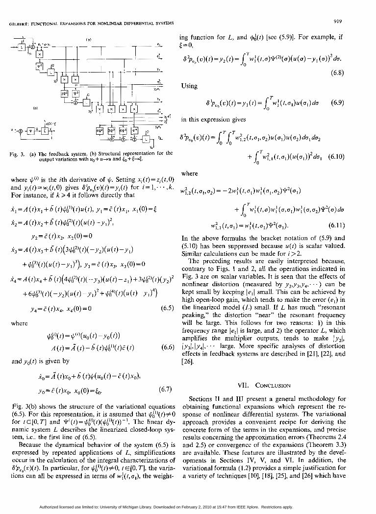
Fig. 3. (a) The feedback system. (b) Structural representation for the output variations with u, + u+u and 5, + (+E.

where

and yo(r) is gven by

Fig. 3(b) shows the structure of the variational equations (6.5). For this representation, it is assumed that $,$’)(t)#O for tE[O, TI and ~i(r )=I+!J~)( t ) ( I+!J~l ’ ( t ) ) - l . The linear dynamic system L describes the linearized closed-loop system, i.e., the first line of (6.5).

Because the dynamical behavior of the system (6.5) is expressed by repeated applications of L, simplifications occur in the calculation of the integral characterizations of 81p,o(c)(t). In particular, for I+!J,$’)(t)#O, t E[O, TI, the variations can all be expressed in terms of wi(t,ul)$ the weight-

ing function for L, and $Act) [see (5.9)]. For example, if t=o,

w:,I(t,‘TI)=)”:(t,uI)\k2(a]). (6.1 1)

In the above formulas the bracket notation of (5.9) and (5. IO) has been suppressed because u( t ) is scalar valued. Similar calculations can be made for i>2.

The preceding results are easily interpreted because, contrary to Figs. 1 and 2, all the operations indicated in Fig. 3 are on scalar variables. It is seen that the effects of nonlinear distortion (measured by y2,y3,y4; . . ) can be kept small by keeping lel( small. This can be achieved by high open-loop gain, which tends to make the error (el) in the linearized model ( L ) small. If L has much “resonant peaking,” the distortion “near” the resonant frequency will be large. This follows for two reasons: 1) in this frequency range lel[ is large, and 2) the operator L, which amplifies the multiplier outputs, tends to make ly21, (y31, Iy4), . . + large. More specific analyses of distortion effects in feedback systems are described in [21], [22], and [ 261.

VII. CONCLUSION

Sections I1 and I11 present a general methodology for obtaining functional expansions which represent the response of nonlinear differential systems. The variational approach provides a convenient recipe for deriving the concrete form of the terms in the expansions, and precise results concerning the approximation errors (Theorems 2.4 and 2.5) or convergence of the expansions (Theorem 3.3) are available. These features are illustrated by the developments in Sections IV, V, and VI. In addition, the variational formula (1.2) provides a simple justification for a variety of techniques [IO], [ 181, [25], and [26] which have


920 IEEE TRANSACTIONS ON AUTOMATIC CONTROL, VOL. AC-22, NO. 6, DECEMBER 1977

been proposed for the derivation of Volterra series. The methodology extends to other types of dynamic systems as well. For instance, discrete-time systems, similar in form to (1.4)-(1.5) or (1.6)-(1.7), can be treated in an analogous fashion [13] and the results of Section VI (e.g.. Fig. 3) can be generalized to the case where L“ is characterized abstractly as a linear, causal operator.

Theorems 4.1-4.4 and 5.1-5.4 give precise conditions on general classes of differential systems which assure the validity of functional expansions. Not surprisingly, these conditions are reminiscent of those which occur in the usual theory of power series. For the system (1.4)-( IS), Theorem 4.4 gives an alternative path to Brockett’s Theo- rem 1 [5], [6] . Theorems 4.2 and 4.3 show that many of the results in [5] are valid whenf,g,h are finitely differentiable instead of analytic in x . Theorems 5.1-5.4 extend these results to the much more general system (1.6) and (1.7). For the special case of stationary systems ( t does not appear in f and h) where xo(t),uo(t) are constant, Theo- rems 5.1-5.4 justify developments which have appeared in many papers and reports [4], [lo], [l 11, [18], [21], [22], [23], [25], [26]. However, in opposition to a frequently expressed belief, the functional expansions are not necessarily Volterra series (see the remarks preceding Theorem 5.1). In [7] the response of bilinear differential systems to initial conditions is characterized; Section V shows that similar characterizations can be obtained for very general nonlinear differential systems. It is worth noting that Theorems llke 4.1-4.4 and 5.1-5.4 can be proved with little modification when the t dependence is more general. For example, in Section V, j , h and u need only be measurable in t if simple integrability conditions are introduced. For k = 1 , Theorems 4.2, 4.3 and 5.2, 5.3 justify rigorously the validity of linear models for nonlinear systems. Such justification is usually neglected; [8], which applies to t E [0, -t cc) instead of t E[O, TI, is an exception.

The form of the variational equations has a number of important implications with respect to the general theory of nonlinear systems, which will be only suggested in what follows. The variations are given exact& by the solution of differential equations of relatively low order (compare with [5]). This is a potential advantage in developing efficient numerical techniques for the evaluation of the kernel functions which appear in the functional expansions. It also shows that if a Volterra series is realizable in the form (1.4)-(1.5), then each term in the series is indi- vidually realizable. This generalizes a conclusion contained in Brockett’s Theorem 4 [5]. Alternative approaches to many other results in [5] follow from the formulas of Section IV. For example, necessary and sufficient conditions that (1.4)-( 1.5) have a finite Volterra series can be given in terms of the A’s, B’s and C’s which appear in (4.7), (4.8), (4.1 I), and (4.12). If it is desired to characterize the variations (4.6) and (4.10) as the solutions of bilinear differential equations, the trick used in the Carle- man bilinearization [5 ] , [17] can be applied to (4.7). (4.Q (4.1 I), and (4.12). To illustrate, the term x:=zl.,. which appears in Fig. 1, can be obtained by solving

i , , , = . f , X x , + x , X i , = ( A x , + B u ) x x ,

+ x , X ( A x , + B u ) = ~ , ~ , z , , , + ~ , , , ( x , X i ; ) ,

which is bilinear in x,,zI,,, and c. This approach differs from [5] in that the bilinear equations give the variations exactly (in [5] there is a remainder term resulting from the truncation of the infinite order Carleman system). Finally, Figs. 1 and 2 can be interpreted as general structural results concerning the realization of nonlinear, causal operators as differential systems. For instance, if an operator is a 2-power of the class (1.6)-(1.7), it can be realized by the first two “layers” of Fig. 1. This realization has similarities with the realization of bilinear operators dis- cussed in [I], [16], and [20]. In fact, the principal results of these papers can be obtained very simply using the tools of Section V 1131.

APPENDIX

Theorem A.1: Assume that f: qn X qrn X [0, TI+’%!’ is continuous and has continuous first partial derivatives with respect to x and u in qn X qrn X[O, TI. Let L% = C([O, TI, am) and ‘3 = c([O. TI, an). Suppose that (1.6) has a solution x, for u = u, E and [ =to E 9 i n . Then there exist constants p > O and K > 0 such that for all u E 9 and (E W satisfying IIu - uoll + l[-[ol < p , 1) the system (1.6) has a solution x € 3, and 2) IIx- xoll <

Proof: Omitted. The general idea is to write an integral equation for i = x - x o and show that for 1 1 u - uoll and 1[-t01 sufficiently small it corresponds to R = T(R) where T is a contraction.

Remark A.2: By an obvious change in notation, Theo- rem A. 1 applies to (1.4).

Remark A.3: For I I u - ~ ~ l l + 1 [ - < ~ 1 <p. it follows that

Remark A.4: The theorem is valid if 9 is replaced by

~ ( l l ~ - u o l l + I t - ~ o l ~ -

IIXII Ko=KP+ llxoll.

e. ACKNOWLEDGMEST

This research was carried out while the author was on leave in the Department of Electrical Engineering, The Johns Hopkins University, Baltimore, MD. Conversations with W. J. Rugh were most helpful.

REFERENCES

[I] M. A. Arbib, “A characterization of multilinear systems,” IEEE

[2] A. V. Balakrishnan. Applied Functional Anaksis. New York: Trans. Auromat. Contr., vol. AC-14, pp. 699-702, 1969.

[3] E. Bedrosian and S. 0. Rice, “The output properties of Volterra Springer Verlag, 1976.

systems driven by harmonic and Gaussian inputs,” Proc. IEEE, vol. 59, pp. 1688-1707, 1971.

[4] M. B. Brilliant, “Theory of the analysis of nodnear systems,” M.I.T. Res. Lab. Electron., Cambridge. MA, Tech. Rep. 345, Mar. 1958.

151 R. W. Brockett, “Volterra series and geometric control theory,”

[6] R. W. Brockett and E. G. Gilbert, “An addendum to Volterra Auromatica, vol. 12. pp. 167-176, 1976.

series and geometric control theory,” Aufomatica, vol. 12, p. 635, 1976.


IEEE TRANSACTIONS ON AUTOOMAT’IC CONTROL, VOL. AC-22, NO. 6, DECEMBER 1977 92 1

[71 C. Bruni, G. DiPillo, and G. Koch, “On the mathematical models of bilinear systems,” Ricerche di Automatica, vol. 2, pp. 11-26,

C. A. Desoer and K. K. Wong, “Small signal behavior of nonlinear 1971.

lumped networks,” Proc. IEEE, vol. 56, pp. 14-22, 1968. J. Dieudonni, Fo~ndations of Modern Analysis. New York: Academic, 1969. R. H. Flake, “Volterra series representation of time-varying nonlinear systems,” in Proc. 2nd Int. IFAC Congr., 1963, pp. 91-99. D. A. George, “Continuous nonlinear systems,” M.I.T. Res. Lab. Electron., Cambridge, MA, Tech. Rep. 355, July 1959. E. G. Gilbert, “Volterra series and the response of nonlinear differential systems: A new approach,” in Proc. of the 1976 Conf. on Information Sciences and System, The Johns Hopkins Univ., Baltimore, MD, pp. 394-400. - “Bilinear and 2-power input-output maps: Finite dimen- sional realizations and the role of functional series,” IEEE Trans. Automat. Contr., to be published, Feb. 1978. L. M. Graves, “Riemann integration and Taylor’s theorem in general analysis,” Trans. Amer. Math. Soc., vol. 29, pp. 163-177, 1927.

Providence, RI: h e r . Math. SOC., 1957. E. Hdle and R. S . Phillips, Functional Anabsis and Semi-Groups.

machines, presented at the IFAC Symp. on Technical and Bio- R. E. K$man, “Pattern recognition properties of multilinear

logical Problems of Control, Yerevan, Armenian SSR, 1968. A. J. Krener, “Linearization and bilinearization of control systems,” in Proc. 1974 Allerton Conf. on Circuit and System Theory, 1974, pp. 834-843. Y. H. Ku and A. A. Wolf, “Volterra-Wiener functionals for the analysis of nonlinear systems,” J . Franklin Imt., vol. 281, pp. 9-26, 1966. S . Lefschetz, Differential Equations: Geometric Theory. New York: Interscience, 1957. G. Marchesini and G. Picci, “Some results on the abstract realization theory of multllinear systems,’’ in Theory and Application of

New York: Academic, 1972, pp. 109-135. Variable Srructure System, R. R. Mohler and A. Ruberti, Ed.

S . Narayanan, “Transistor distortion analysis using Volterra series

[22] S. Narayanan, “Application of Volterra series to intermodulation representation,” Bell Syst. Tech. J . , vol. 4 6 , pp. 991-1023, 1967.

distortion analysis of a transistor feedback amplifier,” IEEE Trans. Circuit Theory, vol. (3T-17, pp. 518-527, 1970.

[23] R. B. Parente, “Nonlinear differential equations and analytic systems theory,” SIAM J . Appl. Math., vol. 18, pp. 41-66, 1970.

[24] W. A. Porter, “An overview of polynomic systems theory,” Proc. IEEE, vol. 64, pp. 18-23, 1976.

[25] K. V.,Rao and R. R ; Mohler, “On the synthesis of Volterra kernels of bllmear systems, Automat. Contr. Theory and Appl., vol. 3, pp.

[26] H. L. Van Trees, “Functional techniques ,$x the analysis of the nodnear behavior of phase-locked loops, Proc. IEEE, vol. 52,

4 4 - 4 6 , 1975.

pp. 894-91 1.

’ c Elmer G. Gilbert was born in Joliet, IL. He received the Ph.D. degree from the University of Michigan, Ann Arbor, in 1957.

Since 1957 he has been on the faculty of the College of Engineering, the University of Michigan, and is now a Professor in the Depart- ment of Aerospace Engineering. Most of his teaching and research activities are in the Com- puter, Information, and Control Engineering Program at Michigan. His most recent leave, 1974-1976, was as a Visiting Professor in the

Department of Electrical Engineering, The Johns Hopkins University, Baltimore, MD. His current research interests are focused in two main areas: optimal periodic control and the theory of nonlinear dynamical systems.

Dr. Gilbert has served on a number of national committees and until this year was a member of the Editorial Board for the SIAM Journal on Control and Optimization.

Convergence of Recursive Adaptive and Identification Procedures Via Weak

Convergence Theory HAROLD J. KUSHNER, FELLOW, IEEE

Abstruct-Results and concepts in the theory of weak convergence of a sequence of probability measures are applied to convergence problem for a variety of recursive adaptive (stochastic approximation-like) methods. Similar techniques have had wide applicability in areas of operations research and in some other areas in stochastic control. It is quite likely that they will play a much more important role in control theory than they do at present, since they allow relatively simple and natural proofs for many types of convergence and approximation problems. Part of the aim of the paper is tutorial: to introduce the ideas and to show how they might be applied. Also, many of the results are new, and they can all be generalized in many directions

recommended by Y. Bar-Shalom, Chairman of the Stochastic Control Manuscript received November 22, 1976; revised April 25, 1977. Paper

Committee. This work was supported in part by the Air Force Office of Scientific Research under Grant AF-AFOSR-76-3063, by the National Science Foundation under Grant Eng-73-03846-A01, and by the Office of Naval Research under Grant NONR NOOO 14-76-C-0279.

in& Brown University, Providence, RI 02912. The author is with the Division of Applied Mathematics and Engineer-

I. INTRODUCTION

HE aims of this paper are twofold. The first aim is T tu to r i a l . The technique of and the results in the theory of weak conoergence of a sequence of probability measures have found many useful applications in many areas of operations research and statistics [l], [2]. Their role in control theory has been relatively limited, being confined mainly to the work in [3], [4] which deals with control problems on diffusion models. Yet, its intrinsic power, as well as the nature of the past successes, suggest that its role in control theory should be deeper than it is at present. The techniques are particularly valuable when convergence or approximation ideas are being dealt with.

In order to illustrate the possibilities, the ideas of weak convergence theory will be applied (the second goal of the


ieee vol. no. december functional expansions …web.eecs.umich.edu/~grizzle/gilbertfest/(36).pdf ·...

Documents