discrete-time reference governors and the nonlinear...

INTERNATIONAL JOURNAL OF ROBUST AND NONLINEAR CONTROL, VOL. 5,487-504 (1995)

DISCRETE-TIME REFERENCE GOVERNORS AND THE NONLINEAR CONTROL OF SYSTEMS WITH STATE AND

CONTROL CONSTRAINTS

ELMER G. GILBERT AND ILYA KOLMANOVSKY Department of Aerospace Engineering, University of Michigan, A m Arbor, Michigan 48109, U.S.A.

AND

KOK TIN TAN Defence Science Organisation. Republic of Singapore, Singapore 0511, Republic of Singapore

SUMMARY

Discrete-time, linear control systems with specified pointwise-in-time constraints, such as those imposed by actuator saturation, are considered. The constraints are enforced by the addition of a nonlinear ‘reference governor’ that attenuates, when necessary, the input commands. Because the constraints are satisfied, the control system remains linear and undesirable response effects such as instability due to saturation are avoided. The nonlinear action of the reference governor is defined in terms of a finitely determined maximal output admissible set and can be implemented on-line for systems of moderately high order. The main result is global in nature: if the input command converges to a statically admissible input and the initial state of the system belongs to the maximal output admissible set, the eventual action of the reference governor is a unit delay.

KEY WORDS nonlinear control; reference governor; control saturation; state constraints

1. INTRODUCTION

Linear models play a vital role in control system design. Powerful design techniques are available for synthesizing controllers which achieve a variety of performance and robustness objectives. Treatment of systems with significant nonlinearities is in a less satisfactory state. Special assumptions concerning the nature of the nonlinearities and the design objectives are needed. This paper addresses the implementation of nonlinear controllers for systems in which the equations of motion are linear but there are pointwise-in-time constraints on control and/or state variables. These assumptions are quite realistic in many practical applications. Certainly, they apply to systems in which the principal nonlinearity is actuator saturation. Our objective is to obtain controllers which preserve desirable small-input behaviour of linear-system designs, respond well to large inputs, have simple structure and, for systems of significant order, can be implemented digitally at reasonably high sampling rates.

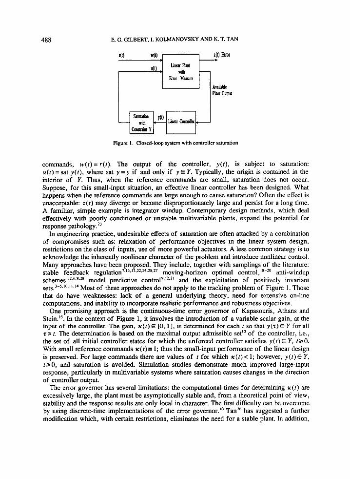
Consider the example system shown in Figure 1. The purpose of feedback control is good tracking performance, i.e., a small closed-loop error, z ( t ) , for a large class of reference

CCC 1049-8923/95/050487-18 0 1995 by John Wiley & Sons, Ltd.

Received 15 February 1994 Revised 12 October 1994

488 E. G. GILBERT, I. KOLMANOVSKY AND K. T. TAN

I , I

Figure I . Closed-loop system with controller saturation

commands, w ( t ) = r ( t ) . The output of the controller, y ( t ) , is subject to saturation: u ( t ) = sat y ( t ) , where sat y = y if and only if y E Y. Typically, the origin is contained in the interior of Y. Thus, when the reference commands are small, saturation does not occur. Suppose, for this small-input situation, an effective linear controller has been designed. What happens when the reference commands are large enough to cause saturation? Often the effect is unacceptable: z ( t ) may diverge or become disproportionately large and persist for a long time. A familiar, simple example is integrator windup. Contemporary design methods, which deal effectively with poorly conditioned or unstable multivariable plants, expand the potential for response path~logy.'~

In engineering practice, undesirable effects of saturation are often attacked by a combination of compromises such as: relaxation of performance objectives in the linear system design, restrictions on the class of inputs, use of more powerful actuators. A less common strategy is to acknowledge the inherently nonlinear character of the problem and introduce nonlinear control. Many approaches have been proposed. They include, together with samplings of the literature: stable feedback regulation7*'3*'7*22.24925*27 moving-horizon optimal control,'"'' anti-windup

.2,6.R92R model predictive contr01~*'~9~' and the exploitation of positively invariant set^.^-'*^"*"*^^ Most of these approaches do not apply to the tracking problem of Figure 1. Those that do have weaknesses: lack of a general underlying theory, need for extensive on-line computations, and inability to incorporate realistic performance and robustness objectives.

One promising approach is the continuous-time error governor of Kapasouris, Athans and Stein.". In the context of Figure 1, it involves the introduction of a variable scalar gain, at the input of the controller. The gain, K ( t ) E [0,1], is determined for each t so that y ( 7 ) E Y for all ta t. The determination is based on the maximal output admissible set'' of the controller, i.e., the set of all initial controller states for which the unforced controller satisfies y ( t ) E Y, t a 0. With small reference commands tc(t)= 1; thus the small-input performance of the linear design is preserved. For large commands there are values of t for which x ( t ) c 1; however, y ( t ) E Y, t B 0, and saturation is avoided. Simulation studies demonstrate much improved large-input response, particularly in multivariable systems where saturation causes changes in the direction of controller output.

The error governor has several limitations: the computational times for determining x ( t ) are excessively large, the plant must be asymptotically stable and, from a theoretical point of view, stability and the response results are only local in character. The first difficulty can be overcome by using discrete-time implementations of the error governor." Tan26 has suggested a further modification which, with certain restrictions, eliminates the need for a stable plant. In addition,

DISCRETE-TIME REFERENCE GOVERNORS 489

he shows that for r ( t )=O his modified error-governor system is asymptotically stable in the large.

In this paper we examine the action of discrete-time reference governors. Figure 2 displays the basic arrangement, reduced to its simplest form. It consists of a controlled process, a pointwise-in-time constraint, y ( t ) E Y, and the reference governor. The purpose of the governor is to attenuate the input command, but only when necessary, so that the constraint is always satisfied. When the controlled process is the closed-loop system of Figure 1, the scheme guarantees that saturation does not take place. Thus, the linear model of the closed-loop system and its performance characteristics remain valid. The nonlinear behaviour of the overall system is determined entirely by the reference governor, whose response characteristics are relatively simple. A key advantage of the approach is that it can be applied to feedback systems which have already been designed for optimum, linear-system performance. Since the reference governor is added after the linear design is complete, compromises need not be made in the linear design process.

Results and developments of the paper are organized as follows. Section 2 formulates the control problem and proposes two discrete-time reference governors, one static and one dynamic. While the static governor is simple and intuitively obvious, it has a somewhat surprising defect: for constant reference commands the output of the reference governor may fail to converge. The dynamic governor, which is the natural discrete-time extension of the continuous-time reference governor of Kapasouris, Athans and Stein,I6 is the principal concern of this paper. Its implementation, which is also based on a maximal output admissible set, is discussed in Section 3. Under appropriate conditions, it is shown that the required nonlinearity can be computed in an efficient and systematic fashion. Section 4 presents results on system response. Unlike others,1n.15.16 they are global in nature. For instance, suppose r ( t ) + ro. where r, is any statically admissible input for the controlled process. Then, w ( t ) + ro. Proofs of the theorems in Section 4 are given in Section 5. Generalizations of the dynamic governor are considered in Section 6. In Section 7 the reference governor is applied to the feedback control of a helicopter which is unstable and has bounds on both of its two inputs. The helicopter with its controller is order 10, so the problem is nonuivial. Large-input responses are good and the instability, which is usually induced by saturation, is avoided. Computational times for the nonlinearities of the reference governor are modest so that on-line implementation is feasible. Section 8 treats an example where the pointwise-in-time constraint is on the output of a closed- loop system. The purpose of the reference governor is to prevent excessive overshoot of the step response. If the state of the controlled process is not available, the reference governor may be implemented with a model of the controlled process. Simulations illustrate the effect of errors in the model.

The following mathematical notation appears: Z' is the set of nonnegative integers; R" and R""" are the usual notations for sets of real vectors and matrices; the superscript T denotes

Figure 2. The reference governor and contmlled process with constrained output


matrix transpose; subscripts indicate vector components; 1x1 is the Euclidean norm of x E R", 1: is the set of bounded sequences, {x(t)E R": tEZ'} (when it is clear by context, we write x E 1:); for x E l:, ~ ~ x ~ ~ ~ = sup( l x ( t ) [ : t E Z + } . The boundary, interior, closure and convex hull of a set are denoted respectively by bd, int, cl and CO. For a E R and X, YC RI', aX={ax: x E X } a n d X + Y = j x + y : x E X , y E Y } .

The discrete-time, maximal output admissible set is defined in terms of a triple, A E R""", C E RI'"" and Y C RI':

O,(A, C, Y) = { x : CA'x E Y, t E Z + } C R" (1)

Obviously, O,(A, C , Y) is related to the system x ( t + 1) = Ax(t ) , y ( t ) = Cx(t). The pointwise-in- time output constraint, y ( t ) E Y, t E Z ' , is satisfied if and only if x(0)E O,(A,C,Y). Our developments depend strongly on results contained in Reference 10. Several are summarized in the following theorem.

Theorem I .1

Suppose A is Lyapunov stable (A' is bounded for all t E Z + ) , Y is compact and 0 E int Y. Then, 0 E int O,(A, C , Y) and O,(A, C , Y) is closed and A invariant (x E O,(A, C, Y) implies Ax E OJA, C , Y)). Suppose, in addition, that C, A is observable. Then, O,(A, C, Y) is compact.

2. THE DISCRETE-TIME REFERENCE GOVERNORS

The controlled process and its constraint, shown in Figure 2, are represented by

x ( t + 1) = h ( t ) + Bw(t ) , X ( t ) E R " , w ( t ) E R " (2)

(3) It is assumed hereafter that: (Al) A has its characteristic roots inside the unit disk, (A2) C, A is observable, (A3) Y is compact and is expressed by

y(t) = Cx(t) + Dw(t ) E Y c R", t E Z+

Y = {y:f,(y)sO, i = 1, ..., s } (4)

where the functions f,: R" + R are continuous and satisfy f, (0) < 0. These assumptions are consistent with constraint modelling of stable closed-loop systems, such as the one shown in Figure 2. Since constraint satisfaction does not depend on states which are unobservable in y, there is no real loss of generality in (A2). The conditions f,(O) < 0 imply 0 E int Y, so that the assumptions of Theorem 1.1 are satisfied. When (2)- (3) represent the system in Figure 2 the constraint is generally state-dependent (C # 0), even though Y is a control constraint.

The constraint set, (4), affects the set of constant inputs for which (2)-(3) has an admissible equilibrium solution. Specifically, w(t)= w, and x ( t ) = x , requires x, = (I - A)-'Bw, and w, E WO, where

w,= {w: H,wE Y} (5 )

(6)

The static reference governor is a scalar gain, K , which varies between 0 and 1 and depends

H, = D + C(Z - A ) - 'B

By assumption (Al) the inverse of I -A exists.

nonlinearly on the reference command and the state of the controlled process:

w( t ) = K ( r ( t ) , x ( t ) > r ( t ) (7)

DISCRETE-TIME REFERENCE GOVERNORS 49 1

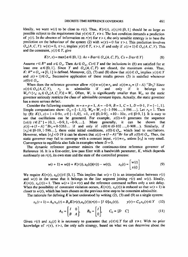
Ideally, we want w( t ) to be close to r ( t ) . Thus, K ( r ( t ) , x ( t ) )E [0,1] should be as large as possible subject to the requirement that y (t) E Y, t 3 t. The last condition demands a prediction of y ( t ) . In the absence of information on r ( t ) for t> t, the only sensible strategy is to base the prediction on the behaviour of the system (2) with w ( t ) = 0 for t> t. This prediction involves O,(A, C, Y): w ( t ) = 0, t> t, implies y(t) E Y, t> t, if and only if x ( t + 1) E O,(A, C, Y). This and the constraint, y ( t ) E Y, give

K(r,x)=max{aE[O,l]: Ax+BarEO,(A,C,Y), C x + D a r E Y ) (8) Assume r E R" and x E 0,. Then Ax E 0,, Cx E Y and the inclusions in (8) are satisfied for at least one a E [0, I]. Since Y and O,(A, C, Y) are closed, the maximum exists. Thus, K: R" x 0, + [0, 1 ] is defined. Moreover, (2), (7) and (8) show that x ( t ) E 0, implies y ( r ) E Y and x ( t + 1) E 0,. Successive application of these results proves (3) is satisfied whenever x ( 0 ) E 0,.

When does the reference governor allow r ( t )= w( t )=rO and x(t)=x,= (Z-A)- 'Bro? Since x ( t ) E O,(A,C, Y), r, is admissible if and only if it belongs to W, n { r,: x, E O,(A, C, Y)) = W,. Often, W, is significantly smaller than WO, so the static governor seriously restricts the class of admissible constant inputs. Actually, the static governor has a more serious defect.

Consider the following example: rn = n = p = 1, A = -0.9, B = 1, C = 1, D = 0.1, Y = [ - 1,1]. Simple computations show: 0, = [ - 1,1], W, = W, = [ - 1-596 . . ., 1-596 . . . I . Let rO = 1. Then by (8): K( l ,x )= 1 +0.9x, xE [-l,O], =1, x E [0,0-9], = l O - lOx, x E [0.9,1]. It is easy to see that oscillations can be generated. For example, x ( O ) = O generates the sequence { x ( t ) : tEZ') = {O,l, -0.9,1, -0.9, ...). More generally, it can be shown that x ( t ) + (I-A)-'BrO=0.5263 ... if and only if x ( 0 ) E (0.102 ..., 0-908 ...). Similarly, if 1 rot E [O. 19,1.596.. .I, there exist initial conditions, x(0) E 0,, which lead to oscillations. However, when I rOl< 0.19 it can be shown that x ( t ) + (I - A)-'Br for all x(0) E 0,. Thus, the static governor may fail to converge with a constant input, r(r)=rO, unless lrol is very small. Convergence to equilibria also fails in examples where D = 0.

The dynamic reference governor mimics the continuous-time reference governor of Reference 16. It is a first-order, low-pass filter with a bandwidth parameter, K, which depends nonlinearly on r ( t ) , its own state and the state of the controlled process:

We require K ( r ( t ) , x G ( t ) ) E [0,1]. This implies that w(t + 1) is an interpolation between r ( t ) and w( t ) in the sense that it belongs to the line segment joining r ( t ) and w(t). Ideally, K ( r ( t ) , x G ( r ) ) = 1. Then w(t + 1) = r ( t ) and the reference command suffers only a unit delay. When the possibility of constraint violation occurs, K ( r ( t ) , x G ( t ) ) is reduced so that w(t + 1) is closer to w(t ) , which has been chosen on the previous time step to be constraint admissible.

The rationale for defining K is best understood by writing (2), (3) and (9) as a single system:

x G ( t + 1) = AGxdt) + BGK(r(t)~G(t))(r(t) - [ I OlxG(t)), r(t) = CGxG(t) E Y (10)

A . = [ ' B A '1, .=[:I, C G = [ D Cl

Given r ( t ) and x G ( t ) it is necessary to guarantee that y ( t ) E Y for all t> t. With no prior knowledge of r ( t ) , z> r , the only safe strategy, based on what we can determine about the


future response of (lO), (1 l) , is to require x(t) E O,(A,, B,, Y), t b t. Then it is known that an acceptable value of K(r(t) , x,(t)), namely 0, is always available. The largest possible value of K(r(t), x,(t)), subject to our requirements, is determined by

K(r,x,)=max[aE [O, 11: A,x,+B,a(r- [ I O]x,)E O,(A,,CG, Y ) } (12)

Note that A, is Lyapunov stable, so the results of Theorem 1.1 apply. Thus, K. R" x O,+ [0, 1 I is defined. Successive applications of (10) and (12) show that x,(O) E 0, implies xG(t) E 0, and y(t) E Y for all r E 2'.

The action of the dynamic governor is quite different from the action of the static governor. Consider the equilibria that can be supported by the dynamic governor. Using the notations introduced previously, it is clear that xGo = [ri xi]T must belong to O,(A,, C,, Y). From (1 l), it can be verified that

From this and the definition of O,(A,, C,, Y) it follows that xGo E O,(A,, C,, Y ) is equivalent to Hero E Y. Hence, the set of admissible ro is WO and there is no additional restriction on the class of constant inputs. Further, as will be seen in Section 4, the convergence difficulties exhibited by the static governor are avoided.

What can be said in general about the behaviour of K in the two governors? Since 0 E int Y and 0 E int 0,, the right sides of (8) and (12) allow a = 1 when r. x and x, are sufficiently small. This and the asymptotic stability of A leads to the following, rather weak, conclusion.

Remark 2.1. For small inputs and initial conditions both governors act as stable linear systems. More specifically, there exists a c>O such that Ilrll,S c and Ix(0)I S c (Ilrll,S c and Ix,(o)l~ c ) imply K ( r ( t ) , x ( t ) ) = 1 ( K ( r ( t ) , xc(t)) = 1) for all t E 2'.

Note that the remark does not contradict the results of the above example for the static governor; it applies if c < 0.19. It will be shown later that a much stronger result holds for the dynamic governor. Because of its inferior response properties, the static reference governor will not be considered further.

3. IMPLEMENTATION OF THE DYNAMIC REFERENCE GOVERNOR

Practical implementation of the dynamic reference governor requires an algorithm for the evaluation of K(r,xG). One is available if O,(A,, C,, Y) is finitely determined," i.e., the infinitely many inequalities appearing in the definition of O,(A,, C,, Y) can be replaced by a finite set of inequalities. When O,(A,, C,, Y) is finitely determined, the listing of the active inequalities has a special structure: I" there exist S" C [ 1, . . . , s } and t,* E Z', i E S', such that

(14)

The index set, S', and the integers, t,*, can be obtained by solving a sequence of mathematical programming problems. Details are given in Reference 10. The computations are often straightforward, even when p , m and n are quite large. For example, when Y is polyhedral the programming problems are linear. Since these computations are only a preliminary step in the determination of K ( r , x,), they are off-line.

O,(A,, C,, Y) = [ x,: fj(CGA',x,) S 0, t = 0, .. ., t,*, i E S*}


Is O,(A,, CG, Y) finitely determined? This question is investigated most easily in a'different coordinate system. Define

1

U = [ 01, A, = u-1AGu, c, = cGu (1 - A)-'B I

Obviously, the indicated inverses exist. It can be verified that

The set O,(A,, CG, Y) is finitely determined if and only if O,(A,, C, Y) is finitely determined. In fact, S* and r,*, i E S', are the same for the two coordinate systems.

Systems of the form (16) are studied in Reference 10. Examples there show that O,(A,, C,, Y) is generally not finitely determined. However, a finitely determined approximation of O,(A,, C,, Y) always exists. This leads to the following theorem.

Theorem 3.1 Suppose the assumptions (AI)- (A3) are satisfied. Define

Proof. First suppose the pair C,, A, is observable. Define

Then by Theorem 5.1 of Reference 10, O,(A,,e,, Y(E) x Y) is finitely determined and O,(A,, C,, Y(E)) C O,(A,, e,, Y ( E ) x Y) C O,(A,, C,, Y). Working these results backward through the state transformation U proves the theorem. The pair C,, A, is observable if and only if rank H, = m, a condition which is not implied by our assumptions. For instance, it fails when m > p. If rank H, < m the proof is camed through by eliminating the unobservable states.

0 See the comments in Section I1 of Reference 10 which concern unobservable systems.

Remark 3.1. The assumption on E implies OEint Y ( E ) + @ . It is also clear that Y ( E ) is compact. Thus, by Theorem 1.1 the sets in (18) are closed, include the origin in their (nonempty) interiors and are A-invariant. They are bounded if and only if rank H,= m. They are convex if Y ( E ) and Y are convex.

To simplify notations define 0:. = OJAG, ec, Y(E) x Y)

The approximation of O,(A,, CG, Y) by 0:. is good in the sense that the 'reduction' of 0:. is no worse than the reduction in O,(A,, CG, Y) which occurs when Y is replaced by Y(E).


Remark 3.2. Ideally, Y(E) + Y (in the HausdorfY metric for compact sets) as E +O. While this property is usually satisfied, it is not guaranteed by assumption (A3). Stronger results are available." If Y is convex, OE int Y and E € [0,1], it is possible to replace Y(E) by (1 - E)Y and O,(AG, CG. Y(E)) by (1 - E)O,(AG, CG, Y)

Clearly, O:={xc:f,(CGAfGxG)sO, r € Z + , f , . ( [ H o O]X,)~-E, i = 1, ..., s ] (21)

Since 0: is finitely determined, only a finite number of the inequalities are active:

Of.={~,:fi(C,A',x,) S O , r = O ,..., r,*, i E S * , f , ( [ H , O]X,)~-E, k = 1 ,..., s ] (22) The special structure of the set of active inequalities is a consequence of Theorem 2.4 in Reference 10. The index sets S* and the r,: depend on E. Usually, the number of inequalities in (22) increases as E becomes smaller. Thus, in choosing E, a compromise must be made between the accuracy of the approximation and the complexity of 0:. Some of the active constraints in (22) may be redundant in the sense that they can be removed from (22) without changing 0:. See Remark 2.2 in Reference 10. Such removal simplifies the computation of K ( r , xG) which is described below.

By Remark 3.1, Of. has the same properties as OJA,, C,, Y). Thus it may replace O,(A,, C,, Y) in the descriptions of Section 2. In particular, K R" x 0 : + [0, 1 ] is defined by

K(r,x,)=max(a€ [0,11: A,xG+B,a(r- [I O]x,)EOE_) (23) Properties of the resulting reference governor are described in the next section.

Expressions (22) and (23) provide the recipe for evaluating K(r , x,):

a j j = m a x ( a E [0, l]:f,(CGA',(A,x,+B,a(r- [ I Olx,)))sOl (24)

a , = m a x { a E [O,l]:fi([Ho O]'A,x,+B,a(r- [I O]X,)))~-E} (25)

(26) K(r,x,)=min(aj,: i E S * , j = O ,..., r,*]u{ai: i = l , ..., s)

By using ( l l ) , (U), (16) and AL = UA',U-l, (24) and (25) can be simplified:

a i=max( a € [0, l]:fi(How+ aH,(r-w))s -E]

D, = D + C(I - A') (I - A) - ' B (28)

(29) Related expressions provide a simple numerical test for xG E 0 L: ~ , € 0 ~ ~ f , ( C A ~ x + D ~ w ) s O , i € S * , j = O ,..., r,*, fk(H,,w)d-~, k = l , ..., s (30)

Actually, (27) and (28) are scalar root-finding problems. In most practical applications, where the functions f j are simple, they have explicit solutions. This is certainly true when Y is a polytope. Then f j ( y ) = yTy - 1, i = 1, . .., s, and

aj j=min{l , (yTDj(r-w)-l(l - yTCA'x- yTDj+ lw) ] , yTDj(r- w)>O

a = min{ 1, (y,TH,,(r - w)-' (1 - E - yTHOw) I , yTHO(r - w) > O = 1, y 'Dj ( r -w)so (31)

= 1, y p l , ( r - w ) < O (32)


Similarly, if f, is a quadratic form, a,, may be expressed in terms of the real roots of a quadratic equation in a.

A few comments are in order. While the evaluation of (26)-(29) is usually straightforward, K ( r , xc) is a complex, piecewise-defined, nonlinear function. Expressions (31) and (32) illustrate the truth of this statement. When Y is a polytope, K: R"' x OC,+ [0, 1 ] is continuous. The proof, based on (26), (31) and (32), is not difficult. The convexity of the polytope does not imply the convexity of K . For real-time implementation of (9) the computation time for K ( r , xG) must be less than T seconds, where T is the sampling interval.

4. RESPONSE PROPERTIES OF THE DYNAMIC REFERENCE GOVERNOR

Our main results on the response properties of the dynamic reference governor are summarized in two theorems. They are stated here, together with remarks pertaining to the nature and significance of their results. Proofs appear in the next section.

The first theorem describes response properties of the reference governor which are independent of the way in which K ( r ( t ) , x G ( t ) ) is determined. Specifically, it concerns the system

(33) w(t + 1) = w ( t ) + K ( t ) ( T ( t ) - w(t))

with K ( t ) E [0, I] .

Theorem 4.1

Assume r E 1: and K: Z'+ [0,1]. Then, the following results hold. (i) w(t)Eco{w(O), r(O), ..., r ( t - l)}. (ii) IIw[I...max[ Iw(O)l, ~ ~ r ~ ~ . . ] . (iii) If r ( t ) has a limit as t + 00, then so does w ( t ) .

All of three conclusions depend crucially on the assumption ~ ( t ) E [0,1]. The first two are simple consequences of it. The third, which is used in the proof of the next theorem, is less evident.

Remark 4.1. Result (i) has an interesting application. Suppose r ( t ) = r,, E R"'. Then w( t ) , tE Z', belongs to the line segment CO( w(O), r,,). Furthermore, because K ( t ) E [0,1], w( t ) progresses monotonically away from w(0) toward r,,. If ~ ( f ) = 1, then w ( t ) = r,,, t > i.

Remark 4.2. For w(0) = 0, (ii) shows that the reference governor is uniformly bounded- input, bounded-output stable with gain bound equal to 1. In Reference 16, bounded-input, bounded-output stability is noted, but no gain bound is given.

Define

WE, = [ w: How E Y ( E ) } = { w: f j (H, ,w) c - E , i = 1, . . . , s } (34)

the set of constant inputs to (2) whose corresponding equilibrium solutions satisfy the constraint y ( r ) E Y ( E ) . From Remark 3.1, WE, is closed and O E int WE,#@. W ; is bounded if and only if rank H,, = m. If Y ( E ) = (1 - E)Y, Wf, = (1 - &)WO.

Theorem 4.2

Consider the system (2), (9) with K defined by (23). Assume: 0 < E < min( - f i (O): i = 1, . . . , s) ,


xG(0)E O:, and r E t! Then the following results hold. (i) For all tEZ': w(t)E W',, x,(t) E 0: and y ( t ) E Y. (ii) Suppose r ( t ) + r , and there exists f E Z' such that r ( t ) E WC, for all r 2 t:, then, there exists ;E Z' such that for all t b t: K ( r ( t ) , x G ( t ) ) = 1. (iii) Suppose r ( t ) + r o and WC,; then, K ( r ( t ) , xG( t ) )+O and w ( t ) - + w * E bdWC,. (iv) Suppose r ( r ) = roE WC,; then, there exists tAEZ'such that for all t a t : K ( r ( t ) , x G ( t ) ) = O and w( t )=w*= w(0)+a4(ro-w(O)),where a*=max(aE[O, l ] : w(O)+a(r,- w(0))E WC,}.

Remark 4.3. Conclusions of the theorem become stronger as E > O becomes smaller. Then, WC, becomes larger and better approximates W,. Usually, the number of inequalities needed to specify 0 : increases as E + 0 and a compromise on the choice of E is necessary.

Remark 4.4. A natural choice for the initial state of the reference governor is w(0) = 0. Then, (1 1 ) and (21) show x,(O) E 0: if and only if x ( 0 ) E OJA, C, Y ) .

Remark 4.5. Suppose WC, is compact (rank Ho = m ) . Then, 1 1 ~ 1 1 . . s c,,,, where c, ,>O is independent of x,(O) and Ilrllm. Thus, for w(O)=O, the Cresponse of the reference governor has a 'saturation' character: 11 wII,< IIrll-, IIwII,< c,,,.

Remark 4.6. Suppose the closed-loop system in Figure 1 is modelled by (2) and (3) and is combined with the reference governor. Then, because of (i), the saturation constraint is inactive and the closed-loop system functions as a linear asymptotically stable system. Furthermore, Remarks 4.2 and 4.5 can be extended to any outputs of the closed-loop system, such as z ( t ) . For example, the zero-state response satisfies ~ ~ z ~ ~ . . ~ k ~ ~ ~ r ~ ~ ~ and IIzII,Lc, where kl and cL are positive constants. It should be emphasized that as an error measure z ( t ) relates plant variables to w(t), not r ( t ) . Error measures based on r(t) are large when r ( t ) - w ( t ) is large.

Remark 4.7. The conclusion in (ii) is strong, considering that it applies to a complex nonlinear system. Since w(t) = r ( t - 1) for t > t: the ultimate response of the overall system is close to that of the linear controlled process. Certainly, (ii) implies convergence to the equilibrium corresponding to ro: w ( t ) + ro and x ( r ) + x g = ( I - A ) -'Bra. Corresponding prior result^'^*'^*'^ on the error and reference governors are much weaker. They depend on the assumption that the governors are always inactive, as in Remark 2.1. The results in (ii) are global in the sense they apply for all convergent sequences, { r ( t ) : r E 2' }, whose elements ultimately belong to WC, and for all xc(0)E 0:. By (21) it follows that w(0) = O and x(0) E O,(A, C, Y ) imply x,(O) E 0:.

Remark 4.8. The assumption in (ii) is about as weak as it can be. Clearly, the result in (ii) cannot hold if ro E W i , for then result (iii) would be violated. Note that the assumption in (ii) is satisfied if r ( t ) = ro E W', or if r ( t ) + ro E intW',. Thus, for ro E W',, the only case not handled by (ii) is the one in which r ( t ) + ro E bdW', and r ( t ) E WC, for infinitely many E Z'. For this case, it can be shown that w( t ) + W* E bdW',, but there is no guarantee that w* = ro.

Remark 4.9. Result (iii) shows that convergence to an equilibrium solution occurs even though ro E W:. The stronger result in (iv) requires r ( t )= ro.

Remark 4.10. The theorem applies under our ovemding assumptions (Al), (A2) and (A3). Thus, Y need not be convex.


5. PROOFS OF THEOREMS

Proof of Theorem 4.1. By (33) and K ( t ) E [0, 11, w(t+ l )Eco{r( t ) , w(t)). Repeated application of this property proves (i). From (i), Iw(t)l dmax{Iw(O)l, lr(0)1, ..., I r ( t - l ) ] ] , which proves (ii). We prove (iii) for m = 1 . This result, applied to the components of w(t) , proves (iii) for m > 1.

Suppose r(t)+r,E R. For E > O , define ; ( E ) so that Ir(r) - r,l d E for all tb t i e ) . Given E > O , there are two possible outcomes: there exists L ( E ) ~ ;(E) such that 1 w ( ~ ( E ) ) - r,,l d E;

I w( t ) - r,, I > E for all t 2 ; ( E ) . Suppose the second outcome holds and w (i( E ) ) > ro + E. Then because x ( i ( ~ ) ) E [ O , l ] and r ( t ( E ) ) d r O + E it follows that r O + ~ < w ( i ( ~ ) + l ) < w ( i ( ~ ) ) . Repeating this argument shows w(r), tb ; ( E ) , is monotone and hence w(t) + w* 2 ro + E.

Similarly, w ( ~ ( E ) ) < ro - E implies w(t) + w* s r,, - E. Thus, we have conclusion (1): w(t) + w* and 1 w* - r,,) b E. If the first outcome holds, (33), K ( ; ( E ) ) E [0,1] and Ir(i(E)) - r,,l d E imply I w(i( E ) + 1) - r,l d E. Repeating this argument leads to conclusion (2): there exists i( E ) such that I w(t) - ro) s E for all t b i( E ) . Thus, for each E > 0 there are the two possible conclusions. If (1) is satisfied for some E > 0, (iii) is proved and w* # r,. If (1) is not satisfied for all E > 0, then (2) implies w ( t ) + ro.

Proof of Theorem 4.2. By (10) and (23), x G ( t ) E 0: implies x , ( t+ l ) E 0:. Thus, x c ( t ) E O:, r E Z'. The remaining conclusions in (i) follow from (21), (4) and (34).

Part (iii) of Theorem 4.1 and the asymptotic stability of A imply x , ( t )+x ;= [ ( w * ) ~ ( x * ) ~ ] ~ , where x * = (Z-A)-'Bw* and, by (i) and the closure of WE,, w* E Wi. From (13), C,A',x*, = How". Thus,

Clearly, y,(t)E Y, t € Z + , and y,(t)+H,w*E Y ( E ) . Since the ff are continuous andf,(H,w*)a - E ,

i E { 1 , . . . , s) , there exists i€ Z' , which is dependent on { r ( t ) : r E Z' ) , xG (0) and E, such that fl(CGA~G.xG(t)) < O for all t b i. Suppose t b i and let xc = x,( t ) and r = r ( t ) in (24). Then from f , ( x c ( t + 1))<0, (10) and (26), it follows that K ( r ( t ) , x G ( t ) ) = a , if and only if all= 1. Thus for r B ?, the a,, contribute nothing to (26) and it may be replaced by

K ( r , x , ) = min{ a,: i E 1 , ..., $1 ] (36) Now consider the proof of (ii). For tb i=max{i , i ) , r ( t ) E WE, and (5.2) applies. Let

w = w ( t ) and r = r ( t ) in (28). Then, a I = 1 , i E { 1 , . . . , s ] and K ( r ( t ) , xG ( t ) ) = 1 for all t 2 i. Theorem 4.1, (i) and Remark 4.4 imply w(t)+ w* E Wi. Thus, for r o e WED, w* # ro. Letting

t + m in (9) proves the first result in (iii). Suppose, contrary to the second result in (iii), that w*EintWi. Then, by (13) and (34), f , ( C , A ' , x ~ ) = f , ( H , w * ) < - ~ , i E { 1 , ..., s]. Because of the strict inequalities, there exist .?>E and ;E Z' such that for all t 2 i, f , (C ,A / ,x , ( t ) )S -2 and f , ( [ H , O]x,(t))d-2. Let x , = x , ( t ) and r = r ( t ) in (24) and (25). Since .?>E and the f, are continuous, there exists an 6 > 0 such that K ( r ( t ) , x , ( t ) )> 8 for all tb i. This, contradicts K ( r ( t ) , x , ( r ) ) + O and the proof of (iii) is complete.

Let w* be given by the expression in (iv). It is obvious from Remark 4.2 that for all t E Z', w(t )Eco~w(O) ,w*]Cco{w(O) ,r , , ] . Again, for t a i , K ( r ( t ) , x , ( t ) ) is determined by (36). Hence, by (28), w(i + 1) = w*. Since further progress toward ro+ w* is impossible,

0 K ( r ( t > , x , ( r ) ) = 0, t> tl= i + 1.

Remark 5.1. The assumption E>O is used in the proof of (ii), (iii) and (iv) and cannot be relaxed even if OJA,, C,, Y ) is finitely determined.


6. ALTERNATIVE DYNAMIC GOVERNORS

A natural alternative to (9) is the dynamic governor introduced by Tan?

w( t + 1) = 1w(t) + K(r ( t ) , x , ( t ) ) ( r ( t ) - 1w(t)) (37)

where O < 1< 1 and AI replaces I in (10) and in the upper left block of A, in (1 1). As in (9) K ( r ( t ) , x G ( t ) ) = 1 implies w ( t + 1) = r ( t ) . Since A, is asymptotically stable, O,(A,, C,, Y ) is finitely determined and the approximation discussed in Section 3 is not needed. Unfortunately, this advantage is overcome by the same disadvantages which haunt the static governor: a reduced set of admissible equilibrium solutions26 and the possibility of steady-state oscillations. The underlying difficulty is in Theorem 4.1; simple examples show that it fails unless 1 = 1. If 1 - 1 is small, simulation studies26 show that the behaviour of (37) is often acceptable and quite similar to (9). However, (37) appears to have no real advantage over (9).

Another alternative to (9) is to replace the scalar valued K by a diagonal matrix and then determine its diagonal elements, K', i = 1, . . . , m, by solving the following, on-line optimization problem: minimize I w( t + 1) - r(t)I2 = I ( I - K ) ( r ( r ) - w(t))I * subject to the constraints O c K ' a l , i = 1, ..., m and A , x , ( t ) + B , K ( r ( t ) - [ I O]x , ( r ) )EO' , (A, ,C, ,Y) . For this alternative, it turns out that parts (ii) and (iii) of Theorem 4.1 and parts (i), (ii) and (iii) of Theorem 4.2 remain valid. The scheme has not been tried. Conceivably, its greater flexibility could offer superior performance.

7. A HELICOPTER WITH CONTROL SATURATION

The controlled process is a tenth-order closed-loop system whose plant is a fourth-order linear model of the vertical dynamics of a helicopter.26 State variables are horizontal and vertical velocity (knots), pitch rate (degrees/s), and pitch angle (degrees). Inputs to the plant are collective pitch, U , , and longitudinal cyclic pitch, u2, measured in degrees. Plant outputs to be controlled are the horizontal and vertical velocities. Zero-order holds with a sampling period, T = 0.1 s., are used at each of the plant inputs The resulting discrete-time model has characteristic roots at: 0-8128, 0-9770, 1.0276 &j0.0265. Clearly, the helicopter is open-loop unstable. Inputs to the controller are the plant outputs and the reference commands. The controller is sixth-order, consisting of an observer-based, stabilizing feedback for the plant and integral control to eliminate steady-state tracking errors. Combining plant and controller dynamics gives a closed-loop system of the form (2)-(3) where y = u . The characteristic roots of A are: 0.3331, 0.4282, 0.5959, 0.9502, 0.6871 *j0.0390,0.5864* j0.4O91,0.9705 f j0.0821.

The two plant inputs saturate at *10 degrees. Thus, f j ( y ) = y j - 10, i = 1 , 2 and f j ( y ) = - y j - 10, i = 3, 4. 0: is determined by solving a sequence of linear programming problems.

Table I. The complexity indices for Of.

0.01 135 159 0-05 88 117 0.1 80 106 0.2 74 97 0.3 56 93

DISCRETE-TIME REFERENCE GOVERNORS

200.0 I I

tu, . 100.0 -

0 .0

-100.0 I -200.0 I I

*0° Wl 400 -400 -LOO 0

Figure 3. Wt for helicopter example

t 20

. . 1 : j 2 0 . 0

0 . 0

-20.0

-40.0

-60.0

6 0 . 0 1 1

................................................ /, ................... 30

-.- 0 5 10 15 20 25 O.lt (b)

499

Figure 4. Horizontal velocity versus time in seconds for several values of ro, (a) No reference governor. (b) With reference governor


1 . 2 c 1 . 2 I L

1 .0

0 . 8

0 . 6

0 .4

0 . 2

0 . 0

4 l )

0 5 O . l t 10

(4 (b)

Figure 5. Reference governor gain versus time in seconds. (a) ro, = 30. (b) rill = 50

The dependence of t ; = t ; and r; = t*, on E is shown in Table I. Large values for t; and t; are not too surprising, since n = 10 and several eigenvalues are close to the unit circle. In addressing the compromise of Remark 4.3, we choose ~ = 0 . 2 . The corresponding set of admissible constant reference commands, Wk, is shown in Figure 3. Since it is quite large, the reduction in equilibrium feasibility is not of great concern. Note that Wi = (1 - &)WO, so the effect of changing E is a simple scale change.

K ( r , x G ) is determined by (26), (31) and (32). Because y3 = -yI and y4 = -y2 , the computational load in (31) and (32) can be reduced by almost a factor of two. On reasonable machines the actual computational time is much less than T = 0.1: for an Apollo DN 400t it is less than 10 milliseconds, for an IBM 6ooo it is less than 2 milliseconds. This is in sharp contrast to the extremely large times needed for continuous-time error and reference governors.

Response results are shown in Figure 4. The initial state of the controlled process is zero and the input is a step command to the horizontal velocity: r , ( t ) = ro,, rz(t)=O. The corresponding horizontal output velocity, v , ( r ) , is plotted. Figure 4 (a) shows what happens when the reference governor is not used and the control variables are allowed to saturate. For ro1 = 20, the system is just below saturation and it behaves as a linear system. For rol = 30, 40, 50, saturation is reached; the instability of the open-loop plant comes into play and the response diverges. Figure 4 (b) shows the corresponding plots when the reference governor, with initial state zero, is added. The response is excellent: well-behaved, only slowing a bit as rol increases. When rol = 20, ~ ( t ) = K ( r ( t ) , x G ( t ) ) = 1. Its behaviour for rol = 30,50 is shown in Figure 5. As predicted by Theorem 4.2, K ( t ) = 1 for ts t: where [depends on ro1. While w,(t) is not shown, its behaviour may be inferred easily from Figure 5 : if ro, = 50, wI (0) jumps to 34 and stays at that level until t = 18 (time= 1.8 seconds) when it begins a slow increase toward 50, arriving therewhen t=46and K ( t ) = 1. Since roz=O, wz(r)=O.

8. A SYSTEM WITH AN OUTPUT CONSTRAINT

In this example the reference governor is used to reduce overshoot in the step response of a single-input, single-output closed-loop system. The open-loop transfer function models a proportional- integral compensator and a plant which has gain c = 1, a four-step transport delay and a first-order lag: G*(z) = 0.15c( l+ 1.7(z - l ) - ' ) ~ - ~ ( l - e-I)(z - e- ' ) - ' . The closed-loop system, with transfer function G*(z)(l + G*(z))-', has an output y ( t ) and is represented by

DISCRETE-TIME REFERENCE GOVERNORS 50 1

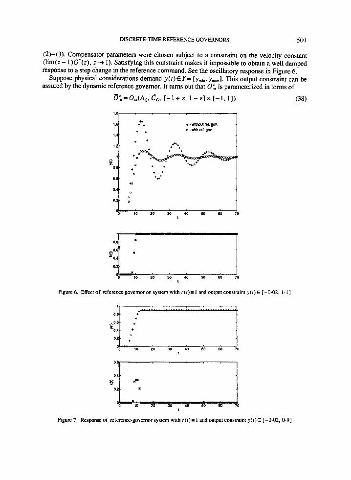
(2)- (3). Compensator parameters were chosen subject to a constraint on the velocity constant (lim(z- l)G*(z), z+ 1). Satisfying this constraint makes it impossible to obtain a well damped response to a step change in the reference command. See the oscillatory response in Figure 6.

Suppose physical considerations demand y ( t ) E Y = [ymin, ymax.. This output constraint can be assured by the dynamic reference governor. It turns out that 0: is parameterized in terms of

(38) D : = o - ( A ~ , C ~ , [-I + E , 1 - E ] x [-1,11)

1.8 I + . withovl rat. gov. o -with ref. gov.

++

1.4 lJ t ++ ++ + +

++*+A

+ + .Y

1.21

+ + + +

0.6 ++++

0.41 0 i I

o o ' l - 1 0 20 30 40 50 60 70 t

1

0.8 ' f I

0.4

'0 10 20 30 40 50 60 70 t

Figure 6. Effect of reference governor on system with r(r)r 1 and output constraint y ( t ) E [-0.02, 1 . 1 1

0 10 20 30 40 50 60 70 t

0.6

0.2

'0 10 20 30 40 50 60 70 t

Figure 7. Response of reference-governor system with r ( t ) i 1 and output constraint y ( t ) E [-0.02, 0.91


Indeed, straightforward manipulations based on (13), (17), (20) and Remark 3.2 show

Once 0: is determined, (23) applied to (39) gives (26) and formulas similar to (31) and (32). The advantage of these steps is that ymin and ymay appear explicitly in the formulas. Since the additional time needed for computing K ( r , x , ) in terms of these parameters is small, they can be changed on-line as process conditions may require. For the results which follow, E = 0-01 and the determination of 0: gives t; = t> = 23. Also, w(0) = 0 and x(0) = 0.

The step response with the governor and Y = [-0.02, 1.11 is shown in Figure 6. For t 2 1 1 , K ( t ) = 1 . Thus, in a remarkably short time the overshoot is reduced to the specified 10 per cent and the system enters its linear regime. Figure 7 shows what happens when Y = [ -0.02, 0..9]. Since r ( t )= l E WC,= [-0-01, 0.891, part (iv) of Theorem 4.2 applies and for r > 13, y ( t ) = 0.89 and ~ ( t ) = 0. Figure 8 illustrates, with Y = [-0.02, 1 - 1 1 , the response properties for a very large oscillatory input which converges to 1. Part (ii) of Theorem 4.2 again applies, but 45 time steps are required before K( t ) = 1.

If the state of the controlled process is not available, or there are errors in the modelling of the controlled process, our results do not apply. A brief empirical investigation of these issues is illustrated in Figure 9. It is assumed that Y = [-0-05, 1-31 and r ( t ) = 1. In the implementation of the reference governor, the state of the controlled process is replaced by the state of a model of the controlled process whose input is w(t ) . If the description of the controlled process and its model are precisely the same and their initial conditions are identical, the reference governor should function as predicted by our theory. This is the case for c = 1 . The remaining responses in Figure 9 show what happens in the presence of modelling errors. The value of c remains equal to 1 in the model but it takes on the values 0-8 and 1.2 in the controlled process. Both responses are certainly much better than the response with no reference governor (cf. Figure 6). However, the limit ymax = 1.3 is violated when c = 1.2. The situation suggests several expedient fixes. One is to reduce ymax below the desired value of 1-3. Another is to carry out the nominal design of the reference governor for c = 1.2 rather than c = 1.

+ I 10 20 30 40 50 60 70

1

0.8

Figure 8. Response of reference-governor system with r ( t ) = 1 + 5e-"-" cos t and output constraint y(r)E [-0.02, 1.11

DISCRETE-TIME REFERENCE GOVERNORS

1.4-

1.2-

1 -

CO.8

0.6

0.4

0.2

503

- -

-

-

+ x x 0 m

X+

0 x-c.1.2 + 0-c-1

+ . c.O.8 X

+

CJ I 0 10 20 30 40 50 60 70

t

Figure 9. Response of model-based, reference-governor system with r (r )a 1 and output constraint y ( r ) E [-0.05, 1.31

9. CONCLUSION Discrete-time reference governors having the configuration shown in Figure 2 have been studied. They enforce the constraint, y ( t ) E Y . t E Z ’ , and thereby avoid undesirable effects of constraint violation such as sluggish response or instability due to actuator saturation. The approach has the distinct advantage that it can be applied to existing, well-designed linear feedback systems. Thus, acceptable large-signal performance can be obtained without sacrificing the small-signal performance of the linear design.

Two governors, one static and the other dynamic, have been considered in detail. The main emphasis is on the dynamic governor because it has superior response characteristics. It is defined by (9), where K is determined by the constraint-predictive property of a maximal output admissible set. For typical constraint sets, K is an easily computed nonlinear function of system state and the reference command. Ease of implementation is a direct consequence of the finite determinability of 0:. Response properties are contained in the theorems and remarks of Section 4. The key result is part (ii) of Theorem 4.2: convergence of the input command to an equilibrium-admissible input implies the existence of fk Z+ such that w ( t ) = r ( t - 1) for all t 3 t: This result is global in character - it applies when there are large reference commands and initial conditions.

Examples confirm the predicted behaviour of the dynamic governor scheme and show that real-time implementations are feasible for systems of moderately high order. State-control constraints other than those imposed by actuator saturation may be treated.

Open questions remain and are being investigated. They include the effects of modelling errors, incomplete measurements of plant state and the treatment of disturbance inputs.

ACKNOWLEDGEMENT

The second author was supported in his work by a FranGois-Xavier Bagnoud doctoral fellowship.

REFERENCES

1. ,ktrom, K. J. , and L. Rundqwist, ‘Integrator windup and how to avoid it’, Proc. 1989 American Contr. Conf., Pittsburgh, PA, 1992, pp. 1693-1698.


2. Astrom, K. J., and B. Wittenmark, Computer Controlled Sysrenu: Theory and Design, 2nd edn, Prentice Hall, Englewood Cliffs, NJ, 1990.

3. Bitsoris, G., ‘Positively invariant polyhedral sets of discrete-time linear systems’, Inr. J . Conrr., 47, 1713-1726 (1988).

4. Bitsoris, G., ‘On the positive invariance of polyhedral sets for discrete-time systems’, Syst. and Conrr. Letters., 11,243-248 (1988).

5. Blanchini, F., ‘Feedback control for linear time-invariant systems with state and control bounds in the presence of disturbances’, IEEE Trans. Automat. Contr., AC-35, 1231-1234 (1990).

6. Campo, F., M. Morari and C. N. Nett, ‘Multivariable anti-windup and bumpless transfer: a general theory’, Proc. 1989American Conrr. Conf.., Pittsburgh, PA, 1989, pp. 1706-1711.

7. Desoer, C. A., and J. Wing, ‘A minimal time discrete system’, IRE Trans. Automat. Contr., AC-6, 111-125 (1961).

8. Doyle, J. C., R. S. Smith and D. F. Enns, ‘Control of plants with input saturation nonlinearities’, Proc. 1987 American Contr. Conf.., Minneapolis, MN, 1987, pp. 1034-1039.

9. Garcia, C. E., D. M. Prett and M. Morari, ‘Model predictive control and practice - a survey’, Auromatica, 25,

10. Gilbert, E. G., and K. T. Tan, ‘Linear systems with state and control constraints: the theory and application of maximal output admissible sets’, IEEE Trans. Automar. Conrr., AC-36, 1008-1020 (1991).

1 1 . Gutman, P.-O., and P. Hagander, ‘A new design of constrained controllers for linear systems’, IEEE Trans. Auromar. Conrr., AC-30, 22-33 (1985).

12. Gutman, P.-O., ‘A linear programming regulator applied to hydroelectric reservoir control’, Auromarica, 22,

13. Gutman, P.-O., and M. Cwikel, ‘An algorithm to find the maximal state constraint sets for discrete-time linear dynamical systems with bounded controls and states’, IEEE Trans. Automat. Contr., AC-32, 251-254 (1987).

14. Hennet, J. C., and J. P. Beziat, ‘A class of invariant regulators for the discrete-time linear regulation problem’, Automarica, 27, 549-554 (1991).

15. Kapasouris, P., M. Athans and G. Stein, ‘Design of feedback control systems for stable plants with saturating actuators’, Proc. IEEE Conf Decision and Control. Austin, TX, 1989, pp. 469-479.

16. Kapasouris, P., M. Athans and G. Stein, ‘Design of feedback control systems for unstable plants with saturating actuators’, Proc. IFAC Symposium on Nonlinear Control System Design, Pergamon Press, Oxford, 1990.

17. Keerthi, S. S., and E. G. Gilbert, ‘Computation of minimum-time feedback control laws for systems with state- control constraints’, IEEE Tram Autornar. Conrr., AC-32,432-435 (1987).

18. Keerthi, S. S., and E. G. Gilbert, ‘Optimal infinite-horizon feedback laws for a general class of constrained discrete-time systems: Stability and moving-horizon approximations’, J. Opt. Theory and Appl., 57, 265-293 (1988).

19. Mayne, D. Q., and H. Michalska, ‘Receding horizon control of nonlinear systems’, IEEE Trans. Auromar. Conrr.,

20. Michalska, H., and D. Q. Mayne, ‘Robust receding horizon control of constrained nonlinear systems’, IEEE Trans. Automat. Contr., AC-38, 1623-1633 (1993).

21. Propoi, A. I., ‘Use of LP methods for synthesizing sampled-data automatic systems’, Auto. Remote Conrr., 24, 837 (1963).

22. Sontag, E. D., and H. J. Sussmann, ‘Nonlinear output feedback design for linear systems with saturating controls’, Proc. IEEE Conf. Decision and Control, Honolulu, HI, 1990, pp. 3414-3416.

23. Stein, G., ‘Respect the unstable’, IEEE Conf. Decision and Conrrol, Hendrik W. Bode Lecture, Tampa, FL, 1989.

24. Sussmann, H. J., and Y. Yang, ‘On the stabilization of multiple integrators by means of bounded feedback controls’, Proc. IEEE Conf Decision and Control. Brighton, England, 1990, pp. 70-73.

25. Sussman, H., E. Sontag and Y. Yang, ‘A general result on the stabilization of linear systems using bounded controls’, Proc. IEEE Conf. Decision and Control, San Antonio, TX, 1993, pp. 1802- 1807.

26. Tan, K. T., ‘Maximal output admissible sets and the nonlinear control of linear discrete-time systems with state and control constraints’, Ph.D. dissertation, Aerospace Engineering, University of Michigan, 1991.

27. Teel, A. R., ‘Global stabilization and restricted tracking for multiple integrators with bounded controls’, Sysr. and Contr. Letrers., 18, 165-171 (1992).

28. Wittenmark, B.. ‘Integrators, nonlinearities, and anti-reset windup for different control structures’, Proc. 1989 American Contr., Conf. .. Pittsburgh, PA, 1989, pp. 1679-1683.

335-348 (1989).

533-541 (1986).

AC-35,814-824 (1990).

discrete-time reference governors and the nonlinear...

Documents