B1. Fourier Analysis of Discrete Time Signals Objectives

• Introduce discrete time periodic signals • Define the Discrete Fourier Series (DFS) expansion of periodic signals • Define the Discrete Fourier Transform (DFT) of signals with finite length • Determine the Discrete Fourier Transform of a complex exponential

1. Introduction In the previous chapter we defined the concept of a signal both in continuous time (analog) and discrete time (digital). Although the time domain is the most natural, since everything (including our own lives) evolves in time, it is not the only possible representation. In this chapter we introduce the concept of expanding a generic signal in terms of elementary signals, such as complex exponentials and sinusoids. This leads to the frequency domain representation of a signal in terms of its Fourier Transform and the concept of frequency spectrum so that we characterize a signal in terms of its frequency components. First we begin with the introduction of periodic signals, which keep repeating in time. For these signals it is fairly easy to determine an expansion in terms of sinusoids and complex exponentials, since these are just particular cases of periodic signals. This is extended to signals of a finite duration which becomes the Discrete Fourier Transform (DFT), one of the most widely used algorithms in Signal Processing. The concepts introduced in this chapter are at the basis of spectral estimation of signals addressed in the next two chapters.

2. Periodic Signals

VIDEO: Periodic Signals (19:45) http://faculty.nps.edu/rcristi/eo3404/b-discrete-fourier-transform/videos/chapter1-seg1_media/chapter1-seg1-

0.wmv

In this section we define a class of discrete time signals called Periodic Signals. There are two reasons why these signals are important:

• A number of signals in nature exhibit periodic repetition. Think of vibrations, ocean waves, seismic waves or electromagnetic waves;

• It is pretty easy to believe that periodic signals are made of (periodic) sinusoids of different frequencies, which is the goal of the Fourier analysis of the rest of the chapter.

Definition: a discrete time signal [ ]x n is periodic if and only if there exists a positive integer

such that

[ ] [ ] for all x n x n N n= + (1)

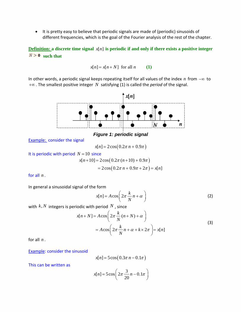
In other words, a periodic signal keeps repeating itself for all values of the index n from −∞ to +∞ . The smallest positive integer N satisfying (1) is called the period of the signal.

Figure 1: periodic signal

Example: consider the signal ( )[ ] 2cos 0.2 0.9x n nπ π= +

It is periodic with period 10N = since ( )( )

[ 10] 2cos 0.2 ( 10) 0.9

2cos 0.2 0.9 2 [ ]

x n n

n x n

π π

π π π

+ = + +

= + + =

for all n . In general a sinusoidal signal of the form

[ ] cos 2 kx n A nN

π α = +

(2)

with ,k N integers is periodic with period N , since

[ ] cos 2 ( )

cos 2 2 [ ]

kx n N A n NN

kA n k x nN

π α

π α π

+ = + + = + + × =

(3)

for all n . Example: consider the sinusoid

( )[ ] 5cos 0.3 0.1x n nπ π= − This can be written as

3[ ] 5cos 2 0.120

x n nπ π = −

Comparing this with (2) we can see that the signal is periodic with period 20N = . In fact we can easily write

( )( )

[ 20] 5cos 0.3 ( 20) 0.1

5cos 0.3 0.1 3 2 [ ]

x n n

n x n

π π

π π π

+ = + −

= − + × =

for all n . In a very similar way a complex exponential of the form

2

[ ]j k n

Nx n Aeπ

= (4)

is periodic with period N since

2 ( )

22

[ ]

[ ]

j k n NN

j k njkN

x n N Ae

Ae e x n

π

ππ

+

+ =

= × =

Example: consider the complex exponential 0.1[ ] (1 2 ) j nx n j e π= +

This can be written as 1220[ ] (1 2 )

j nx n j e

π = +

and it is periodic with period 20N = .

3. Expansion of Periodic Signals: the Discrete Fourier Series (DFS).

VIDEO: Reference Frames (21:25) http://faculty.nps.edu/rcristi/eo3404/b-discrete-fourier-transform/videos/chapter1-seg1_media/chapter1-seg1-

1.wmv

Now the problem we want to address is to determine a “reference frame” for discrete time periodic signals. In other words the issue is to determine a set of periodic signals which serve as a basis of any other periodic signal. The concept of a “reference frame” is very important in a number of fields, including geometry, navigation and signal processing. It extends simple, intuitive geometric ideas to more complex abstract problems. Going back to geometry, recall that, given a vector x we can represent it in terms of a reference frame defined by:

• An origin “0”; • Reference vectors 1 2, ,...e e

Figure 2 below shows an example of a vector in the plane.

Figure 2: a vector and a reference frame in the plane

Given this definition we can see that a vector (say) in the plane is always represented by the components along the directions of the basis vectors. In this case, as shown in figure 3, the vector x is represented as shown in figure 3 as 1 1 2 2x a e a e= +

where

• 1a is the projection of the vector x along 1e • 2a is the projection of the vector x along 2e

Figure 3: vector representation in terms of its projections on the reference frame

For example you want to locate yourself with respect to a reference point and you say that you are 300m East and 200m North of your reference. In this case the reference vectors 1 2,e e are in the East and North directions respectively, of unit length (1 meter) and the components 1 2,a a of your position are 300m and 200m respectively. This is shown in figure 4.

Figure 4: example of a geographical position as a vector in the Earth reference

frame.

For signals we use a very similar concept. We want to express any arbitrary signal [ ]x n as the sum of reference signals having appropriate physical properties, significant for our problems. In our case and in a lot of applications, the reference signals are sinusoids or complex exponentials, as shown in figure 5.

Figure 5: a signal as a sum of reference signals

Given any periodic signal with period N a very attractive set of reference candidates is the set of complex exponentials with the same period N . These are defined as

2

[ ] , 0,..., 1kj nN

ke n e k Nπ

= = − (5) It turns out that we can show the following Fact: any discrete time periodic signal with period N can be written as

1

0[ ] [ ]

N

k kk

x n a e n−

=

=∑

for some constants 0 1 1, ,... Na a a − . Example: take the periodic signal shown in figure 6 below. It is easy to see that it is periodic with period 2N = , since it keeps repeating the value 1,2,1,2,… periodically.

Figure 6: periodic signal with period 2N =

Since the period is 2N = the reference exponentials [ ]ke n in (5) are given by

022

0122

1

[ ] 1 1

[ ] ( 1)

j n n

j n n

e n e

e n e

π

π

= = =

= = −

We can easily verify (try to believe!) that the given periodic signal in figure 6 can be written as

0 1[ ] 1.5 [ ] 0.5 [ ]

1.5 1 0.5 ( 1)n n

x n e n e n= +

= × − × −

In fact this expression yields [ ] 1.5 0.5 1x n = − = for n even and [ ] 1.5 0.5 2x n = + = for n odd.

Example: consider another example of a periodic signal with period 2N = shown in figure 7.

Figure 7: periodic signal with period 2N =

Again we use the same reference signals [ ]ke n , 0,1k = defined as

022

0122

1

[ ] 1 1

[ ] ( 1)

j n n

j n n

e n e

e n e

π

π

= = =

= = −

It can be easily verified that this signal can be written as 0 1[ ] 0.5 [ ] 0.8 [ ]

0.5 1 0.8 ( 1)n n

x n e n e n= +

= × + × −

4. Orthogonality of the Reference Signals

VIDEO: Orthogonal Reference Signals (20:52) http://faculty.nps.edu/rcristi/eo3404/b-discrete-fourier-transform/videos/chapter1-seg2_media/chapter1-seg2-

0.wmv

From the simple geometric examples in the previous section (figures 2,3,4) we see that the vectors in the reference frames are orthogonal to each other. It turns out that this makes it easier in determining the expansion of the vectors in terms of reference frames. A very similar approach extends to reference signals. In particular we can verify that the

complex exponentials 2

[ ]jk n

Nke n e

π

= are all “orthogonal” to each other in the sense that

1

*

0

0 if [ ] [ ]

if

N

k mn

m ke n e n

N m k

−

=

≠= =

∑ (6)

This is easy to show just by applying the definition of complex exponentials as follows:

1 1 12 2*

0 0 0[ ] [ ]

nm k m kN N Nj n jN N

k mn n n

e n e n e eπ π− −− − −

= = =

= =

∑ ∑ ∑ (7)

Now we can apply the geometric sum, defined as

1

0

1 if 11

if 1

NN

n

n N

α αα αα

−

=

−≠= −

=∑ (8)

with 2 m kj

Neπ

α−

= . Then applying (7) to (8) we obtain the orthogonality condition in (6). The fact that the complex exponentials [ ]ke n are orthogonal as in (6) makes the computation of the expansion coefficients ka a very simple matter. In fact, let [ ]x n be a periodic signal with period N and let’s write it again as

1

0[ ] [ ]

N

k kk

x n a e n−

=

=∑

Then, the N coefficients 0 1 1, ,..., Na a a − of the expansion can be easily computed from the orthogonality of the complex exponentials as

1 1 1 1 1

* * *

0 0 0 0 0

[ ]

[ ] [ ] [ ] [ ] [ ] [ ]N N N N N

k m m k m k m kn n m m n

x n

x n e n a e n e n a e n e n Na− − − − −

= = = = =

= = =

∑ ∑ ∑ ∑ ∑

VIDEO: Discrete Fourier Series (16:08) http://faculty.nps.edu/rcristi/eo3404/b-discrete-fourier-transform/videos/chapter1-seg2_media/chapter1-seg2-

1.wmv

The rightmost expression comes from the orthogonality property, for which the summation is nonzero only when k m= . It is customary to define [ ] kX k Na= for 0,..., 1k N= − and call it the Discrete Fourier Series (DFS) of the periodic sequence [ ]x n . This can be computed as

{ }21

0[ ] [ ] [ ] , 0,..., 1

N j knN

nX k DFS x n x n e k N

π− −

=

= = = −∑ (9)

Conversely, the original the signal [ ]x n is called the Inverse Discrete Fourier Series (IDFS) and it can be written as

{ }21

0

1[ ] [ ] [ ]N j kn

N

kx n IDFS X k X k e

N

π−

=

= = ∑ (10)

Example Revisited: consider the example we have seen above (figure 6), with period 2N = . Then the Discrete Fourier Series (DFS) of the given signal is computed as

212

0[ ] [ ] [0] [1]( 1) 1 2 ( 1) , 0,1

j nk k k

nX k x n e x x k

π−

=

= = + − = + × − =∑

Therefore this yields [0] 3X = and [1] 1X = − . The given signal can then be expressed as

{ }212

0

1[ ] [ ] [ ] 1.5 0.5 ( 1)2

j kn n

kx n IDFS X k X k e

π

=

= = = − × −∑

same as in the example above.

Example: Consider the periodic signal [ ]x n shown in figure 8 below.

Figure 8: a periodic signal with period 10N = .

Then we compute its Discrete Fourier Series (DFS) as

2 510

2 29 4210 1010

0 0

1 if 1, 2,...,9[ ] [ ]15 if 0

j k

j kn j knj k

n n

e kX k x n e ee

k

π

π ππ

−

− −−

= =

− == = = −

=

∑ ∑

This sequence can be plotted in terms of magnitude and phase as

Figure 9: DFS of the signal in figure 8

Example: Let the signal [ ]x n be defined as

[ ] 2 cos(0.5 )x n nπ= It is periodic and let’s see what the period is. Just compute a few values to obtain

[0] 2, [1] 0,x x= = [2] 2, [3] 0,...x x= = This shows that the period is 2N = , which yields its DFS as

212

0[ ] [ ] [0] [1] ( 1) , 0,1

j kn k

nX k x n e x x k

π−

=

= = + × − =∑

Substituting for [0], [1]x x we obtain [0] [1] 2X X= = .

5. Signals of a Finite Length and the Discrete Fourier Transform (DFT)

VIDEO: the Discrete Fourier Transform (12:20) http://faculty.nps.edu/rcristi/eo3404/b-discrete-fourier-transform/videos/chapter1-seg3_media/chapter1-seg3-

0.wmv

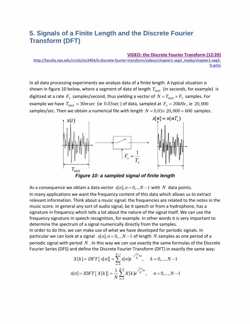
In all data processing experiments we analyze data of a finite length. A typical situation is shown in figure 10 below, where a segment of data of length MAXT (in seconds, for example) is digitized at a rate SF samples/second, thus yielding a vector of MAX SN T F= × samples. For example we have 30 secMAXT m= (ie 0.03sec ) of data, sampled at 20SF kHz= , ie 20,000samples/sec. Then we obtain a numerical file with length 0.03 20,000 600N = × = samples.

Figure 10: a sampled signal of finite length

As a consequence we obtain a data vector [ ], 0,... 1x n n N= − with N data points. In many applications we want the frequency content of this data which allows us to extract relevant information. Think about a music signal: the frequencies are related to the notes in the music score. In general any sort of audio signal, be it speech or from a hydrophone, has a signature in frequency which tells a lot about the nature of the signal itself. We can use the frequency signature in speech recognition, for example. In other words it is very important to determine the spectrum of a signal numerically directly from the samples. In order to do this, we can make use of what we have developed for periodic signals. In particular we can look at a signal [ ], 0,... 1x n n N= − of length N samples as one period of a periodic signal with period N . In this way we can use exactly the same formulas of the Discrete Fourier Series (DFS) and define the Discrete Fourier Transform (DFT) in exactly the same way:

{ }21

0[ ] [ ] [ ] , 0,..., 1

N j knN

nX k DFT x n x n e k N

π− −

=

= = = −∑

{ }21

0

1[ ] [ ] [ ] , 0,..., 1N j kn

N

nx n IDFT X k X k e n N

N

π−

=

= = = −∑

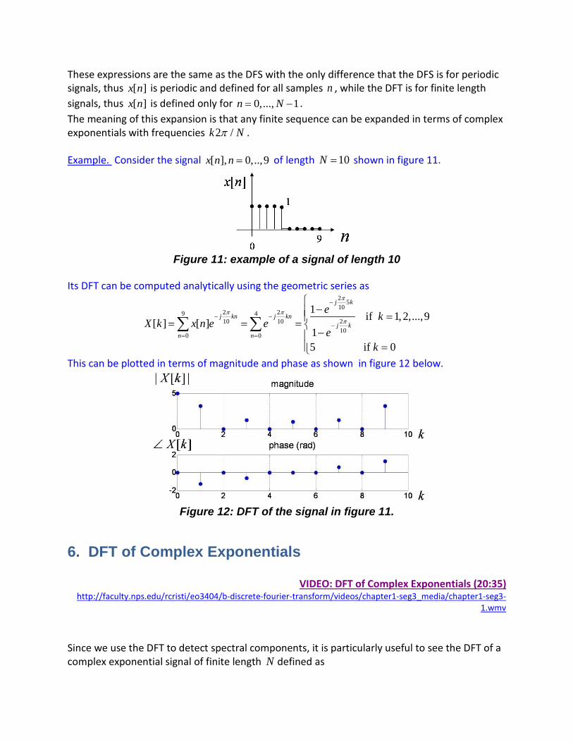
These expressions are the same as the DFS with the only difference that the DFS is for periodic signals, thus [ ]x n is periodic and defined for all samples n , while the DFT is for finite length signals, thus [ ]x n is defined only for 0,..., 1n N= − . The meaning of this expansion is that any finite sequence can be expanded in terms of complex exponentials with frequencies 2 /k Nπ . Example. Consider the signal [ ], 0,..,9x n n = of length 10N = shown in figure 11.

Figure 11: example of a signal of length 10

Its DFT can be computed analytically using the geometric series as

2 510

2 29 4210 1010

0 0

1 if 1, 2,...,9[ ] [ ]15 if 0

j k

j kn j knj k

n n

e kX k x n e ee

k

π

π ππ

−

− −−

= =

− == = = −

=

∑ ∑

This can be plotted in terms of magnitude and phase as shown in figure 12 below.

Figure 12: DFT of the signal in figure 11.

6. DFT of Complex Exponentials

VIDEO: DFT of Complex Exponentials (20:35) http://faculty.nps.edu/rcristi/eo3404/b-discrete-fourier-transform/videos/chapter1-seg3_media/chapter1-seg3-

1.wmv

Since we use the DFT to detect spectral components, it is particularly useful to see the DFT of a complex exponential signal of finite length N defined as

0[ ] , 0,... 1j nx n Ae n Nω= = − where 0ω represents the digital frequency in radians. Applying the definition of its DFT we obtain the following expression

{ }

00

21

0

221 1

0 0

[ ] [ ] [ ]

, 0,..., 1

N j knN

n

N N j k nj knj n NN

n n

X k DFT x n x n e

Ae e Ae k N

π

ππ ωω

− −

=

− − − −−

= =

= =

= = = −

∑

∑ ∑

Notice that this expression has a particular structure and it can be written in the following way:

02[ ] NX k A W kNπ ω = × −

where the function ( )NW ω depends only on the data length N and it is defined as

1

0

1( )1

j NNj n

N jn

eW ee

ωω

ωω−−

−−

=

−= =

−∑

Again the variable ω indicates digital frequency and it is in radians. As we will show below, the same expression can be written in a different way as

( 1)/2sin

2( )sin

2

j NN

N

W e ω

ω

ωω

− −

=

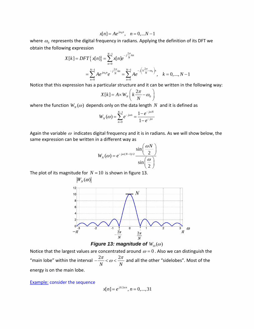
The plot of its magnitude for 10N = is shown in figure 13.

Figure 13: magnitude of 10 ( )W ω

Notice that the largest values are concentrated around 0ω = . Also we can distinguish the

“main lobe” within the interval 2 2N Nπ πω− < < and all the other “sidelobes”. Most of the

energy is on the main lobe. Example: consider the sequence

0.3[ ] , 0,...,31j nx n e nπ= =

In this case 0 0.3 , 32Nω π= = . Then its DFT becomes

( ) 23232

[ ] 0.3 , 0,...,31k

X k W kπωω π

== − =

In order to see how this looks like, let’s plot first ( )32 0.3W ω π− as in figure 14

Figure 14: plot of ( )32 0.3W ω π−

Then, to see its DFT, we take samples as { } ( ) 2

32[ ] [ ] 0.3 , 0,...,31N k

X k DFT x n W kπωω π

== = − =

This is shown in figure 15.

Figure 15: DFT of the example. Notice that the maximum corresponds to the index 5k = which yields the digital frequency 5 2 / 32 0.312 0.3ω π π π= × = ≅

7. The Fast Fourier Transform in Matlab One of the most important reason (if not the most important) reasons why the DFT has become a very popular algorithm is the extremely high efficiency of its implementation. In particular the Fast Fourier Transform (FFT) can compute the DFT of a large data set in a very short time. Just to give an idea, if we have N data points, and N is a power of 2, we can compute its DFT in an amount of time proportional to NN 2log , using the FFT, versus 2N by “brute force”

computation. For example let (say) 1024210 ==N . Then the time taken by the FFT is proportional to 3

2 101024log1024 ≅ , while the brute force approach would take an amount of time proportional to 62 101024 ≅ . As a consequence, all computer applications, including Matlab, use the FFT rather then the DFT. The results of both operations are identical, but the FFT computes it in a fraction of the time taken by the brute force DFT.

VIDEO: FFT in Matlab (20:43) http://faculty.nps.edu/rcristi/eo3404/b-discrete-fourier-transform/videos/chapter1-seg4_media/chapter1-

seg4.wmv

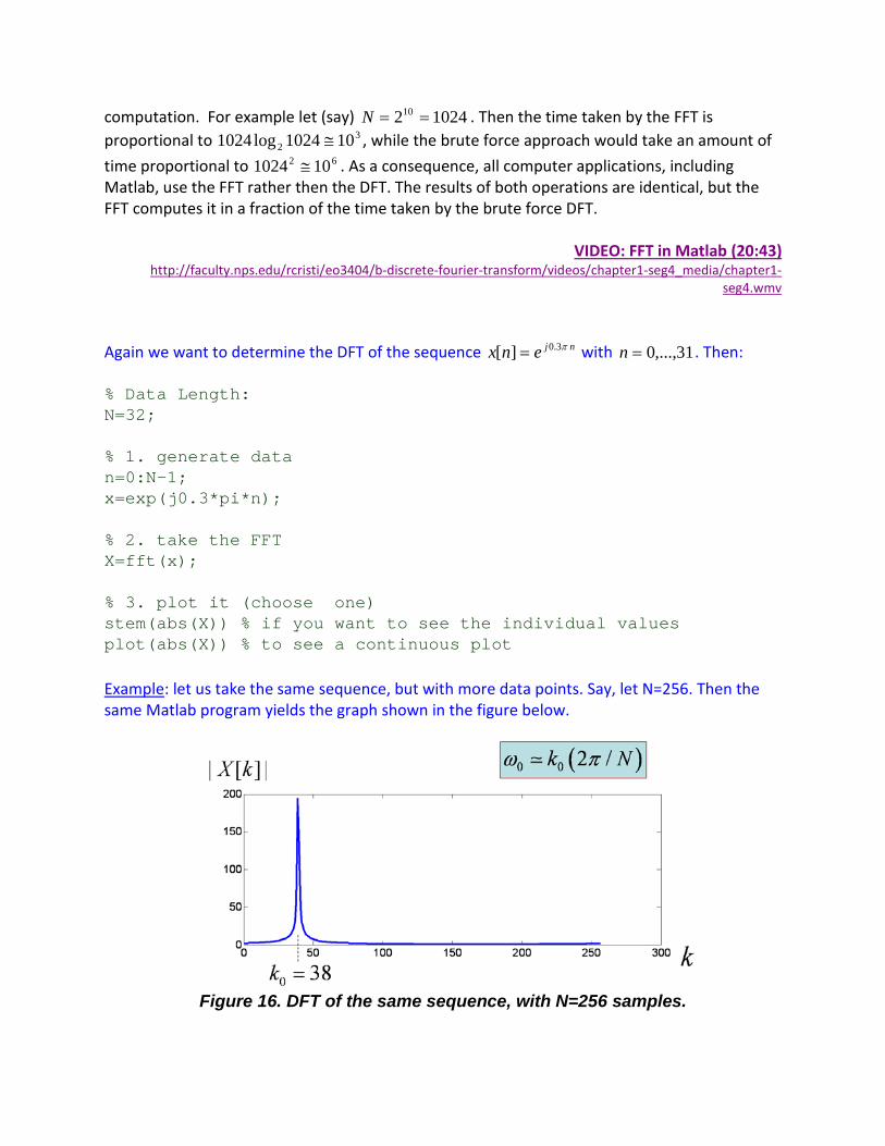
Again we want to determine the DFT of the sequence njenx π3.0][ = with 31,...,0=n . Then: % Data Length: N=32; % 1. generate data n=0:N-1; x=exp(j0.3*pi*n); % 2. take the FFT X=fft(x); % 3. plot it (choose one) stem(abs(X)) % if you want to see the individual values plot(abs(X)) % to see a continuous plot Example: let us take the same sequence, but with more data points. Say, let N=256. Then the same Matlab program yields the graph shown in the figure below.

Figure 16. DFT of the same sequence, with N=256 samples.

The peak can be verified to be at 38=k so that the estimated frequency is

πππω 3.02969.0256238 ≅==

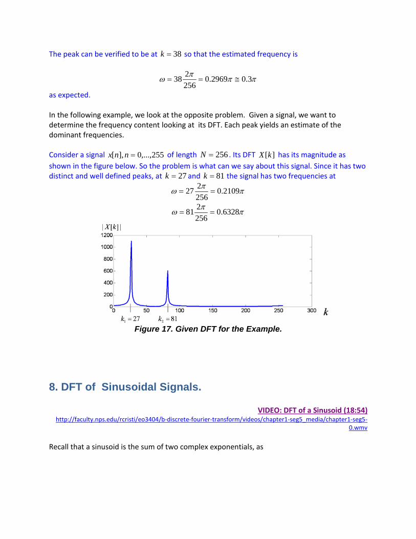
as expected. In the following example, we look at the opposite problem. Given a signal, we want to determine the frequency content looking at its DFT. Each peak yields an estimate of the dominant frequencies. Consider a signal 255,...,0],[ =nnx of length 256=N . Its DFT ][kX has its magnitude as shown in the figure below. So the problem is what can we say about this signal. Since it has two distinct and well defined peaks, at 27=k and 81=k the signal has two frequencies at

ππω 2109.0256227 ==

ππω 6328.0256281 ==

Figure 17. Given DFT for the Example.

8. DFT of Sinusoidal Signals.

VIDEO: DFT of a Sinusoid (18:54) http://faculty.nps.edu/rcristi/eo3404/b-discrete-fourier-transform/videos/chapter1-seg5_media/chapter1-seg5-

0.wmv

Recall that a sinusoid is the sum of two complex exponentials, as

( ) njjnjj eeAeeAnAnx 00

22cos][ 0

ωαωααω −−

+

=+=

In the spectral domain it is represented as two frequencies as shown in the figure below.

Figure 18. Spectral Representation of a Sinusoid

Now we want to see what is its DFT when we take a finite data length 1,...,0],[ −= Nnnx . Define again { }][][ nxDFTkX = and since it is the sum of two complex exponentials, its DFT is the sum of the respective DFT’s, as

+

= −− njjnjj eeADFTeeADFTkX 00

22][ ωαωα

The rightmost term, with negative frequency 0ω− requires some consideration since the frequencies 1,...,0,/2 −= NkNk π computed by the DFT cannot be negative. We can easily see that njnj ee )2( 00 ωπω −− = , with 02 0 ≥−ωπ so that the above DFT becomes

+

= −− njjnjj eeADFTeeADFTkX )2( 00

22][ ωπαωα

The two frequencies 0ω and 02 ωπ − are shown in the figure below.

Figure 19. Frequency domain representation of a sinusoidal signal, using positive

frequencies only.

As a consequence of this, the DFT of a sinusoidal signal at frequency πω << 00 is going to show two peaks: one at 0ω and one at 02 ωπ − . Both components have the same magnitude

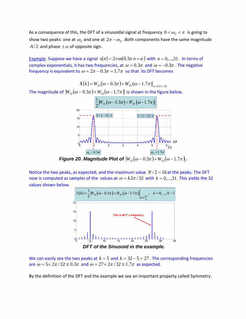
2/A and phase α± of opposite sign. Example. Suppose we have a signal ( )απ += nnx 3.0cos2][ with 31,...,0=n . In terms of complex exponentials, it has two frequencies, at πω 3.0= and πω 3.0−= . The negative frequency is equivalent to πππω 7.13.02 =−= so that its DFT becomes

( )32/23232 )7.1(3.0][

πωπωπω

kWWkX

=−+−=

The magnitude of ( ) ( )πωπω 7.13.0 3232 −+− WW is shown in the figure below.

Figure 20. Magnitude Plot of ( ) ( )πωπω 7.13.0 3232 −+− WW .

Notice the two peaks, as expected, and the maximum value 162/ =N at the peaks. The DFT now is computed as samples of the values at 32/2πω k= with 31,...,0=k . This yields the 32 values shown below.

DFT of the Sinusoid in the example.

We can easily see the two peaks at 5=k and 27532 =−=k . The corresponding frequencies are ππω 3.032/25 ≅×= and ππω 7.132/227 ≅×= as expected. By the definition of the DFT and the example we see an important property called Symmetry.

VIDEO: Symmetry of the DFT (09:22) http://faculty.nps.edu/rcristi/eo3404/b-discrete-fourier-transform/videos/chapter1-seg5_media/chapter1-seg5-

1.wmv

Symmetry of the DFT. Given a real signal 1,...,0],[ −= Nnnx , its DFT { } 1,...,0,][][ −== NknxDFTkX is such that

][][ * kXkNX =− Proof. From the definition of the DFT replacing the index k with kN − we obtain

∑∑−

=

−

=

−−==−

1

0

21

0

)(2

][][][N

n

knN

jN

n

nkNN

jenxenxkNX

ππ

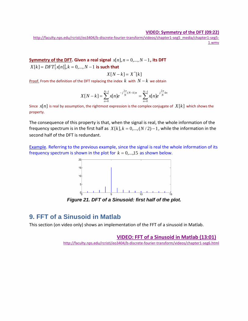
Since ][nx is real by assumption, the rightmost expression is the complex conjugate of ][kX which shows the property. The consequence of this property is that, when the signal is real, the whole information of the frequency spectrum is in the first half as 1)2/(,...,0],[ −= NkkX , while the information in the second half of the DFT is redundant. Example. Referring to the previous example, since the signal is real the whole information of its frequency spectrum is shown in the plot for 15,...,0=k as shown below.

Figure 21. DFT of a Sinusoid: first half of the plot.

9. FFT of a Sinusoid in Matlab This section (on video only) shows an implementation of the FFT of a sinusoid in Matlab. VIDEO: FFT of a Sinusoid in Matlab (13:01)

http://faculty.nps.edu/rcristi/eo3404/b-discrete-fourier-transform/videos/chapter1-seg6.html