advanced leak detection using a nonlinear observer and olga
TRANSCRIPT
8/18/2019 Advanced Leak Detection using a Nonlinear Observer and OLGA
http://slidepdf.com/reader/full/advanced-leak-detection-using-a-nonlinear-observer-and-olga 1/131
June 2007
Ole Morten Aamo, ITK
Master of Science in Engineering CyberneticsSubmission date:
Supervisor:
Norwegian University of Science and Technology
Department of Engineering Cybernetics
Advanced leak detection in oil and gaspipelines using a nonlinear observerand OLGA models
Espen Hauge

8/18/2019 Advanced Leak Detection using a Nonlinear Observer and OLGA
http://slidepdf.com/reader/full/advanced-leak-detection-using-a-nonlinear-observer-and-olga 2/131
8/18/2019 Advanced Leak Detection using a Nonlinear Observer and OLGA
http://slidepdf.com/reader/full/advanced-leak-detection-using-a-nonlinear-observer-and-olga 3/131
Problem Description
The subject originates from the requirement of monitoring pipelines carrying oil and gas. Statoiloperates several pipelines, for instance between Kollsnes and Mongstad. A system for supervision
of these pipelines is imposed by the authorities. This system must incorporate a thorough model,enabling among others Mongstad to predict the production rate and detect leakages. The thesis isbased on earlier submitted projects and theses where methods of detecting leaks have beentested under nominal conditions with a simplified model. That is why this thesis shall focus onproper modelling and robustness with regard to modelling error and biased measurements. Thethesis is performed in collaboration with Statoil’s R&D center at Rotvoll. The following subjectsare to be considered:
1. Outline earlier work done in the special field of leak detection and motivate for further work.2. Define a one-phase flow in a straight, horizontal pipeline (should be a fairly simple case to easedebugging), and implement with OLGA. The earlier constructed Matlab observer should be testedwith data from OLGA and compared with an observer designed in OLGA. Cases with bothstationary and non-stationary flow should be tested.3. Document the procedure of setting up an OLGA observer.4. Test the leak detection system constructed with OLGA with data produced with OLGA and wherethere are no modelling errors. (The observer should be an exact copy of the model.) Performancewith both stationary and non-stationary flow should be examined. How does this compare toearlier results?5. Design an OLGA observer for a pipeline with varying altitude and commit similar tests as above.6. Define and carry out a systematic study of robustness with regard to modelling errors andbiased measurements with stationary boundary conditions.a. The modelling error should originate from a set of chosen parameters, and the observer shouldconsist of fewer segments than the model.b. Details regarding biased measurements are provided by Statoil.7. Make suggestions for further work – consider the possibility of developing a leak detection
system for two-phase flow.8. Write a conference article to NOLCOS 2007 (7th IFAC Symposium on Nonlinear ControlSystems)9. Write a journal article to SPE Journal.
Assignment given: 08. January 2007Supervisor: Ole Morten Aamo, ITK

8/18/2019 Advanced Leak Detection using a Nonlinear Observer and OLGA
http://slidepdf.com/reader/full/advanced-leak-detection-using-a-nonlinear-observer-and-olga 4/131
8/18/2019 Advanced Leak Detection using a Nonlinear Observer and OLGA
http://slidepdf.com/reader/full/advanced-leak-detection-using-a-nonlinear-observer-and-olga 5/131
i
Summary
An adaptive Luenberger-type observer with the purpose of locating and quantifyingleakages is presented. The observer only needs measurements of velocity and temperature
at the inlet and pressure at the outlet to function. The beneficial effect of outputinjection in form of boundary conditions is utilized to ensure fast convergence of theobserver error. This approach is different from the usual practice where output injectionmight appear as a part of the PDE’s. This makes it possible to employ OLGA, whichis a state of the art computational fluid dynamics simulator, to govern the one-phasefluid flow of the observer. Using OLGA as a base for the simulations introduces thepossibility to incorporate temperature dynamics in the simulations which in previouswork was impossible. The observer is tested with both a straight, horizontal pipelineand an actual, long pipeline with difference in altitude. Both simulations with oil andgas are carried out and verification of the robustness of the observer is emphasized. Inorder to cope with modelling errors and biased measurements, estimation of roughness
in the monitored pipeline is introduced.

8/18/2019 Advanced Leak Detection using a Nonlinear Observer and OLGA
http://slidepdf.com/reader/full/advanced-leak-detection-using-a-nonlinear-observer-and-olga 6/131
ii
8/18/2019 Advanced Leak Detection using a Nonlinear Observer and OLGA
http://slidepdf.com/reader/full/advanced-leak-detection-using-a-nonlinear-observer-and-olga 7/131
iii
Preface
This work is the result of the Master of Science thesis performed at the department of engineering cybernetics at the Norwegian University of Science and Technology (NTNU)
during the period from January ’07 until June ’07. The thesis is a collaboration betweenNTNU and Statoil R&D, department of process control, at Rotvoll, Trondheim.
I would like to thank my advisor at Statoil, John-Morten Godhavn, and especially myadvisor at NTNU, Ole Morten Aamo.

8/18/2019 Advanced Leak Detection using a Nonlinear Observer and OLGA
http://slidepdf.com/reader/full/advanced-leak-detection-using-a-nonlinear-observer-and-olga 8/131
iv
8/18/2019 Advanced Leak Detection using a Nonlinear Observer and OLGA
http://slidepdf.com/reader/full/advanced-leak-detection-using-a-nonlinear-observer-and-olga 9/131
1
Contents
Summary i
Preface iii
List of Figures 5
List of Tables 7
1 Introduction 9
2 Previous work 11
3 Theory 13
3.1 Mathematical Model used in Matlab . . . . . . . . . . . . . . . . . . . . . 133.1.1 Physical Model . . . . . . . . . . . . . . . . . . . . . . . . . . . . . 13
3.1.2 Characteristic Form . . . . . . . . . . . . . . . . . . . . . . . . . . 14
3.1.3 Observer Design . . . . . . . . . . . . . . . . . . . . . . . . . . . . 15
3.1.4 Adaption of friction coefficient . . . . . . . . . . . . . . . . . . . . 17
3.1.5 Leak Detection . . . . . . . . . . . . . . . . . . . . . . . . . . . . . 17
3.1.6 Remodelling the leak . . . . . . . . . . . . . . . . . . . . . . . . . . 183.1.7 Summary . . . . . . . . . . . . . . . . . . . . . . . . . . . . . . . . 20
3.2 The OLGA simulator . . . . . . . . . . . . . . . . . . . . . . . . . . . . . . 21
3.2.1 The connection between OLGA and Matlab . . . . . . . . . . . . . 21
3.2.2 Friction adaption with OLGA . . . . . . . . . . . . . . . . . . . . . 21
3.2.3 Estimation of leak parameters with OLGA . . . . . . . . . . . . . 22
4 Method 23
4.1 Numerical solution in Matlab . . . . . . . . . . . . . . . . . . . . . . . . . 23
4.2 Distributing the leak over two nodes . . . . . . . . . . . . . . . . . . . . . 25
4.3 Computing pressures and density at point of leak . . . . . . . . . . . . . . 27
4.4 Setting up an OLGA observer . . . . . . . . . . . . . . . . . . . . . . . . . 28
4.4.1 Obtaining correct measurements . . . . . . . . . . . . . . . . . . . 28
4.4.2 Controlling the boundaries . . . . . . . . . . . . . . . . . . . . . . 30
8/18/2019 Advanced Leak Detection using a Nonlinear Observer and OLGA
http://slidepdf.com/reader/full/advanced-leak-detection-using-a-nonlinear-observer-and-olga 10/131
2 CONTENTS
4.4.3 Controlling the leakages . . . . . . . . . . . . . . . . . . . . . . . . 304.4.4 Adjusting the time step . . . . . . . . . . . . . . . . . . . . . . . . 31
4.5 Verification test of the valve equation . . . . . . . . . . . . . . . . . . . . 324.6 Estimating mass rate of leak . . . . . . . . . . . . . . . . . . . . . . . . . 32
4.7 Adaption of friction coefficients . . . . . . . . . . . . . . . . . . . . . . . . 334.8 Tuning of update laws . . . . . . . . . . . . . . . . . . . . . . . . . . . . . 334.9 Multiple observers . . . . . . . . . . . . . . . . . . . . . . . . . . . . . . . 34
4.10 Computing mean values . . . . . . . . . . . . . . . . . . . . . . . . . . . . 344.11 Computing time of convergence . . . . . . . . . . . . . . . . . . . . . . . . 34
4.12 Computing the L2 norm of the observer error . . . . . . . . . . . . . . . . 35
5 Results 375.1 Output injection . . . . . . . . . . . . . . . . . . . . . . . . . . . . . . . . 37
5.2 Friction adaption with OLGA . . . . . . . . . . . . . . . . . . . . . . . . . 395.3 Verification of the valve equation . . . . . . . . . . . . . . . . . . . . . . . 40
5.4 Comparison of the Matlab and OLGA observer . . . . . . . . . . . . . . . 405.4.1 Stationary flow . . . . . . . . . . . . . . . . . . . . . . . . . . . . . 415.4.2 Sinusoidal varying boundaries . . . . . . . . . . . . . . . . . . . . . 46
5.4.3 Shut down . . . . . . . . . . . . . . . . . . . . . . . . . . . . . . . 505.4.4 Summary . . . . . . . . . . . . . . . . . . . . . . . . . . . . . . . . 54
5.5 Simulations with gas and temperature dynamics . . . . . . . . . . . . . . 555.6 Multiple observers . . . . . . . . . . . . . . . . . . . . . . . . . . . . . . . 62
5.6.1 Comments . . . . . . . . . . . . . . . . . . . . . . . . . . . . . . . . 67
5.7 Robustness . . . . . . . . . . . . . . . . . . . . . . . . . . . . . . . . . . . 68
5.7.1 Biased measurements . . . . . . . . . . . . . . . . . . . . . . . . . 685.7.2 Difference in grid size . . . . . . . . . . . . . . . . . . . . . . . . . 72
5.8 Time-varying boundaries . . . . . . . . . . . . . . . . . . . . . . . . . . . . 755.9 Estimation of mass rate . . . . . . . . . . . . . . . . . . . . . . . . . . . . 82
5.10 Tor 1 carrying gas . . . . . . . . . . . . . . . . . . . . . . . . . . . . . . . 835.11 Discussion . . . . . . . . . . . . . . . . . . . . . . . . . . . . . . . . . . . . 85
5.11.1 Future work . . . . . . . . . . . . . . . . . . . . . . . . . . . . . . . 88
6 Conclusions 89
References 91
A Simulation parameters 93A.1 Matlab observer . . . . . . . . . . . . . . . . . . . . . . . . . . . . . . . . 93
A.2 OLGA models . . . . . . . . . . . . . . . . . . . . . . . . . . . . . . . . . . 94A.2.1 Straight pipe . . . . . . . . . . . . . . . . . . . . . . . . . . . . . . 94A.2.2 Tor . . . . . . . . . . . . . . . . . . . . . . . . . . . . . . . . . . . . 94
A.3 OLGA observers . . . . . . . . . . . . . . . . . . . . . . . . . . . . . . . . 95A.3.1 Straight pipe . . . . . . . . . . . . . . . . . . . . . . . . . . . . . . 95
A.3.2 Tor . . . . . . . . . . . . . . . . . . . . . . . . . . . . . . . . . . . . 95

8/18/2019 Advanced Leak Detection using a Nonlinear Observer and OLGA
http://slidepdf.com/reader/full/advanced-leak-detection-using-a-nonlinear-observer-and-olga 11/131
Contents 3
B Additional plots 97
C Proof 100C.1 Uniform grid size for positive leak distribution . . . . . . . . . . . . . . . 100
D Article 103

8/18/2019 Advanced Leak Detection using a Nonlinear Observer and OLGA
http://slidepdf.com/reader/full/advanced-leak-detection-using-a-nonlinear-observer-and-olga 12/131
4 CONTENTS
8/18/2019 Advanced Leak Detection using a Nonlinear Observer and OLGA
http://slidepdf.com/reader/full/advanced-leak-detection-using-a-nonlinear-observer-and-olga 13/131
5
List of Figures
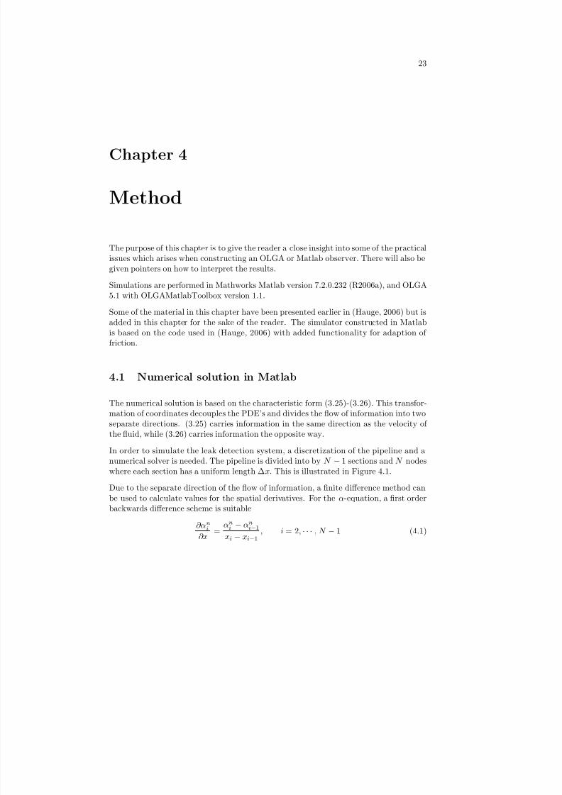
4.1 Discretization of the pipeline. . . . . . . . . . . . . . . . . . . . . . . . . . 24
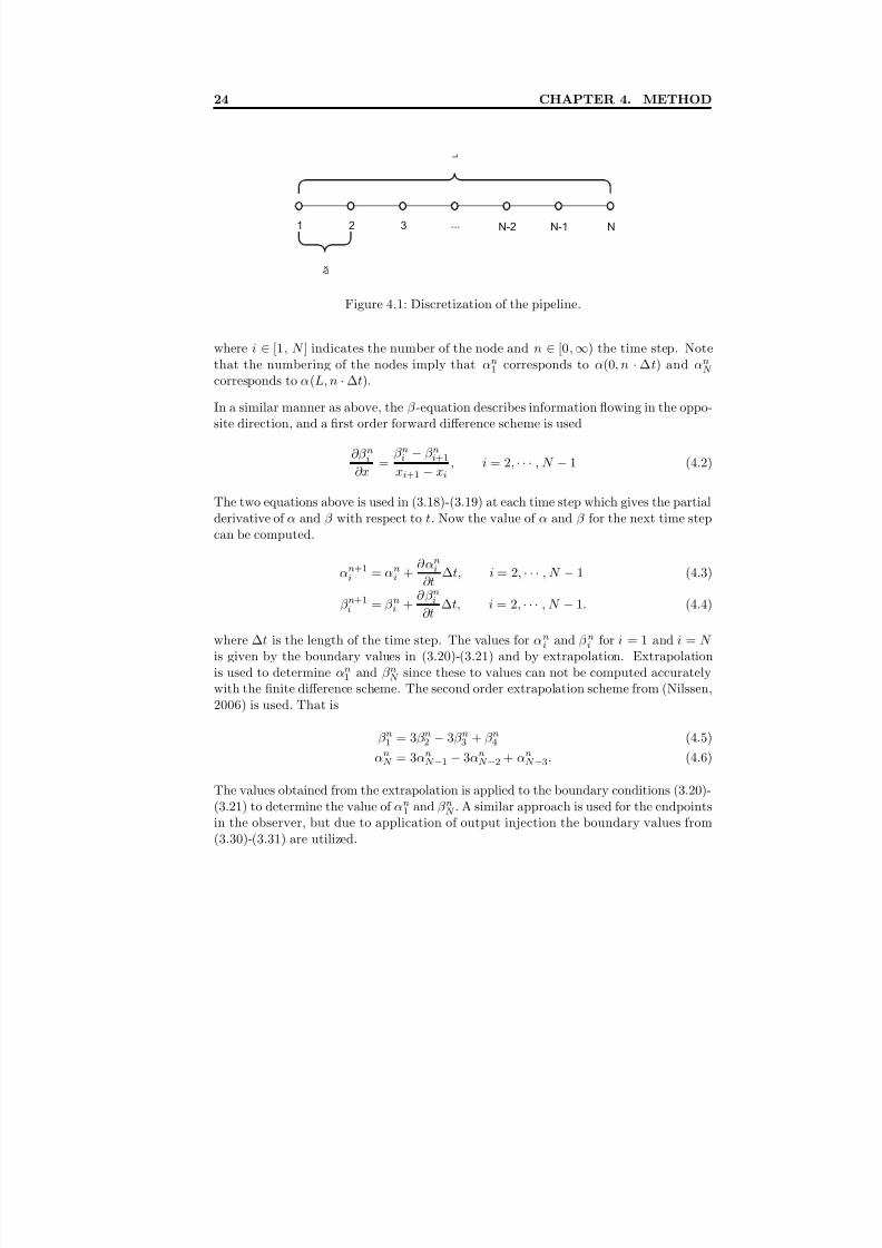
4.2 Sketch of the distribution of the leak. . . . . . . . . . . . . . . . . . . . . . 25
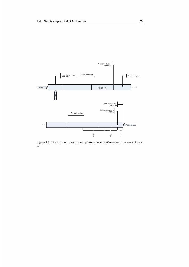
4.3 The situation of source and pressure node relative to measurements of pand u. . . . . . . . . . . . . . . . . . . . . . . . . . . . . . . . . . . . . . . 29
5.1 Oil, stationary. The effect of output injection. . . . . . . . . . . . . . . 38
5.2 Oil, stationary. Friction adaption with the OLGA observer with andwithout temperature dynamics. . . . . . . . . . . . . . . . . . . . . . . . . 39
5.3 Gas, stationary. Friction adaption with the OLGA observer with andwithout temperature dynamics. . . . . . . . . . . . . . . . . . . . . . . . . 39
5.4 The ratio between computed control signal and the actual control signal. . 40
5.5 Oil, stationary. Estimates for a leak at 850 m. . . . . . . . . . . . . . . 42
5.6 Gas, stationary. Estimates for a leak at 850 m. . . . . . . . . . . . . . . 43
5.7 Oil, stationary. Estimates for a leak at 4650 m. . . . . . . . . . . . . . . 44
5.8 Gas, stationary. Estimates for a leak at 4650 m. . . . . . . . . . . . . . 45
5.9 Oil, sinusoid. Measurements from OLGA of the boundaries with a leakat 3450 m. . . . . . . . . . . . . . . . . . . . . . . . . . . . . . . . . . . . . 46
5.10 Oil, sinusoid. Estimates for a leak at 3450 m. . . . . . . . . . . . . . . . 47
5.11 Gas, sinusoid. Measurements from OLGA of the boundaries with a leakat 3450 m. . . . . . . . . . . . . . . . . . . . . . . . . . . . . . . . . . . . . 48
5.12 Gas, sinusoid. Estimates for a leak at 3450 m. . . . . . . . . . . . . . . 49
5.13 Oil, shut down. Measurements from OLGA of the boundaries with aleak at 1350 m. . . . . . . . . . . . . . . . . . . . . . . . . . . . . . . . . . 50
5.14 Oil, shut down. Estimates for a leak at 1350 m. . . . . . . . . . . . . . 515.15 Gas, shut down. Measurements from OLGA of the boundaries with aleak at 1350 m. . . . . . . . . . . . . . . . . . . . . . . . . . . . . . . . . . 52
5.16 Gas, shut down. Estimates for a leak at 1350 m. . . . . . . . . . . . . . 53
5.17 Gas, stationary. Estimation of roughness for an observer with temper-ature dynamics turned on. The estimation is turned off after 2 minutesdue to the occurrence of a leak. . . . . . . . . . . . . . . . . . . . . . . . . 56
5.18 Gas, stationary. Estimates for a leak at 1550 m. . . . . . . . . . . . . . 57
5.19 Gas, sinusoid. Sinusoidal varying boundaries for a leak at 750 m. . . . . 58
8/18/2019 Advanced Leak Detection using a Nonlinear Observer and OLGA
http://slidepdf.com/reader/full/advanced-leak-detection-using-a-nonlinear-observer-and-olga 14/131
6 LIST OF FIGURES
5.20 Gas, sinusoid. Estimates for a leak at 750 m. . . . . . . . . . . . . . . . 595.21 Gas, shut down. The boundaries during a shut down for a leak at 3850
m. . . . . . . . . . . . . . . . . . . . . . . . . . . . . . . . . . . . . . . . . 605.22 Gas, shut down. Estimates for a leak at 3850 m. . . . . . . . . . . . . . 615.23 Profile of the Tor 1 pipeline with point of leaks marked with arrows and
observer starting points marked with callout boxes. . . . . . . . . . . . . . 635.24 Oil, stationary. Estimates for a leak at 23884 m. The leak magnitude
is 3.3 % of the mass rate at the inlet . . . . . . . . . . . . . . . . . . . . . 735.25 Oil, stationary. Estimates for a leak at 65790 m. The leak magnitude
is 1.2 % of the mass rate at the inlet . . . . . . . . . . . . . . . . . . . . . 745.26 Oil, shut down. Observer boundaries during a shut down with a leak
at 21664 m. . . . . . . . . . . . . . . . . . . . . . . . . . . . . . . . . . . . 765.27 Oil, shut down. Observer error during a shut down with a leak at 21664
m. . . . . . . . . . . . . . . . . . . . . . . . . . . . . . . . . . . . . . . . . 765.28 Oil, shut down. Estimates during a shut down with a leak at 21664 m. 775.29 Oil, start up. Observer boundaries during a start up with a leak at 5758
m. . . . . . . . . . . . . . . . . . . . . . . . . . . . . . . . . . . . . . . . . 785.30 Oil, start up. Observer error during a start up with a leak at 5758 m. . 785.31 Oil, start up. Estimates during a start up with a leak at 5758 m. . . . . 795.32 Oil, sinusoid. Observer boundaries varying as sinusoids with a leak at
5758 m. . . . . . . . . . . . . . . . . . . . . . . . . . . . . . . . . . . . . . 805.33 Oil, sinusoid. Observer error with a leak at 5758 m. . . . . . . . . . . . 805.34 Oil, sinusoid. Estimates for sinusoidal varying boundary conditions with
a leak at 5758 m. . . . . . . . . . . . . . . . . . . . . . . . . . . . . . . . . 81
5.35 Oil, stationary. Comparison of estimations of C v and wl. . . . . . . . . 825.36 Gas, stationary. The boundaries of the observer for a leak at 8709 m. . 835.37 Gas, stationary. Observer error with gas flow and a leak at 8709 m. . . 835.38 Gas, stationary. A failed attempt to locate a leak at 8709 m. . . . . . . 84
B.1 Oil, stationary. Estimates of the friction coefficient, ∆, for leaks at both850 m and 4650 m. . . . . . . . . . . . . . . . . . . . . . . . . . . . . . . . 97
B.2 Gas, stationary. Estimates of the friction coefficient, ∆, for leaks atboth 850 m and 4650 m. . . . . . . . . . . . . . . . . . . . . . . . . . . . . 98
B.3 Oil, sinusoid. Estimates of the friction coefficient, ∆, for a leak a leakat 3450 m. . . . . . . . . . . . . . . . . . . . . . . . . . . . . . . . . . . . . 98
B.4 Gas, sinusoid. Estimates of the friction coefficient, ∆, for a leak at 3450m. . . . . . . . . . . . . . . . . . . . . . . . . . . . . . . . . . . . . . . . . 98
B.5 Oil, shut down. Estimates of the friction coefficient, ∆, for a leak at1350 m. . . . . . . . . . . . . . . . . . . . . . . . . . . . . . . . . . . . . . 99
B.6 Gas, shut down. Estimates of the friction coefficient, ∆, for a leak at1350 m. . . . . . . . . . . . . . . . . . . . . . . . . . . . . . . . . . . . . . 99
8/18/2019 Advanced Leak Detection using a Nonlinear Observer and OLGA
http://slidepdf.com/reader/full/advanced-leak-detection-using-a-nonlinear-observer-and-olga 15/131
7
List of Tables
5.1 Stationary. Leak magnitudes . . . . . . . . . . . . . . . . . . . . . . . . 41
5.2 Sinusoid. Leak magnitudes . . . . . . . . . . . . . . . . . . . . . . . . . . 46
5.3 Shut down. Leak magnitudes . . . . . . . . . . . . . . . . . . . . . . . . 50
5.4 Summary of the results for the comparison of the Matlab and OLGAobserver. . . . . . . . . . . . . . . . . . . . . . . . . . . . . . . . . . . . . . 54
5.5 Maximum and minimum of leak magnitude in percent of the initial massflow. . . . . . . . . . . . . . . . . . . . . . . . . . . . . . . . . . . . . . . . 55
5.6 Summary table, leakage with gas flow and temperature dynamics. . . . . 55
5.7 Tuning and starting point of leak for the observers with ambient pressuredepending on depth. . . . . . . . . . . . . . . . . . . . . . . . . . . . . . . 62
5.8 Tuning and starting point of leak for the observers with uniform back-pressure at each leak. . . . . . . . . . . . . . . . . . . . . . . . . . . . . . . 62
5.9 Observer 1. Summary of simulations. . . . . . . . . . . . . . . . . . . . . 64
5.10 Observer 2. Summary of simulations. . . . . . . . . . . . . . . . . . . . . 65
5.11 Observer 5. Summary of simulations. . . . . . . . . . . . . . . . . . . . . 65
5.12 Observer 3. Summary of simulations. . . . . . . . . . . . . . . . . . . . . 66
5.13 Observer 6. Summary of simulations. . . . . . . . . . . . . . . . . . . . . 66
5.14 Observer 4. Summary of simulations. . . . . . . . . . . . . . . . . . . . . 67
5.15 Observer 7. Summary of simulations. . . . . . . . . . . . . . . . . . . . . 67
5.16 The expected biases of the measured signals from the model. . . . . . . . 68
5.17 A small bias added to the mass rate without estimation of roughness. . . 69
5.18 A small bias added to the mass rate with estimation of roughness. . . . . 69
5.19 A relatively large bias added to the mass rate without estimation of rough-
ness. . . . . . . . . . . . . . . . . . . . . . . . . . . . . . . . . . . . . . . . 705.20 A relatively large bias added to the mass rate with estimation of roughness. 70
5.21 Perturbing pressure without estimation of the roughness. . . . . . . . . . 70
5.22 Perturbing pressure with estimation of roughness. . . . . . . . . . . . . . . 71
5.23 Perturbing temperature without estimation of roughness. . . . . . . . . . 71
5.24 Perturbing temperature with estimation of roughness. . . . . . . . . . . . 71
5.25 Summary table for the comparison of various observers with model error. 72
5.26 Time varying boundary conditions, magnitude of leakages . . . . . . . . . 75
5.27 Time varying boundary condtitions, summary table . . . . . . . . . . . . 75

8/18/2019 Advanced Leak Detection using a Nonlinear Observer and OLGA
http://slidepdf.com/reader/full/advanced-leak-detection-using-a-nonlinear-observer-and-olga 16/131
8 LIST OF TABLES
A.1 Pipeline and fluid parameters for the Matlab observer for a horizontalpipeline. . . . . . . . . . . . . . . . . . . . . . . . . . . . . . . . . . . . . . 93
A.2 Tuning parameters for the Matlab observer. . . . . . . . . . . . . . . . . . 93A.3 Pipeline parameters for the OLGA model without inclinations. . . . . . . 94A.4 Pipeline parameters for the OLGA model of the Tor pipeline. . . . . . . . 94A.5 Tuning for the straight pipe OLGA observer. . . . . . . . . . . . . . . . . 95A.6 Tuning of update laws for the robustness study. . . . . . . . . . . . . . . . 95A.7 Tuning of update laws for the cases with model error. . . . . . . . . . . . 95A.8 Tuning of update laws for the cases with time-varying boundaries. . . . . 96A.9 Observer parameters for estimation of C v vs wl. . . . . . . . . . . . . . . . 96A.10 Observer parameters for estimation during gas flow with the Tor 1 pipeline. 96
8/18/2019 Advanced Leak Detection using a Nonlinear Observer and OLGA
http://slidepdf.com/reader/full/advanced-leak-detection-using-a-nonlinear-observer-and-olga 17/131
9
Chapter 1
Introduction
Leak detection based on dynamic modelling is a propitious approach in the special fieldof leak quantification and location. This report documents one of the first real stepstoward a new method of pipeline monitoring. A state of the art multiphase simulatoris manipulated through Matlab to work as an adaptive Luenberger-type observer whichuses measurements from the supervised pipeline as well as internal measurements. Thisobserver is capable of handling modelling errors and disturbances, as opposed to open-loop observers, due to the use of output injection and estimation of friction. Since theonly measurements fed into the observer are pressure and velocity measurements fromthe inlet and outlet, which in most cases already are available, the method can be used
with most existing pipelines without extra instrumentation. Also, the computationalfluid dynamics simulator, which is the backbone of the observer, is a widely used one,namely OLGA.1 Many of the existing pipelines have already been modeled in OLGAwhich can be exploited in the construction of the observer.
The benefits of a leak detection system able of locating the position of the leak within aquantified tolerance are obviously of an environmental kind. But the economical aspectof it is also important since it may be the determining factor when new technology istaken into practice. Another advantage of this kind of method would be that it undersome circumstances can be used after a leak has been detected and the pipeline hasbeen shut down. This is possible by logging the relevant measurements and running
simulations with the observer with the stored model data. It is also be possible to havemultiple observers with different tuning and starting point monitoring a pipeline duringoperation.
The work done in this thesis is based on the previous work done in (Hauge, 2006)where the pipeline flow was simulated by a Matlab model based on two coupled onedimensional first order nonlinear hyperbolic partial differential equations. This modelis recapitulated in the theory section, and also mentioned in the method section for the
1OLGA is developed by IFE, Sintef, Statoil and Scandpower Petroleum Technology
8/18/2019 Advanced Leak Detection using a Nonlinear Observer and OLGA
http://slidepdf.com/reader/full/advanced-leak-detection-using-a-nonlinear-observer-and-olga 18/131
10 CHAPTER 1. INTRODUCTION
sake of the reader. The update laws of the observer are based on this model and arestrictly heuristic.
Whereas the previous computational fluid dynamics simulator written in Matlab didnot incorporate an energy equation or support pipelines with difference in altitude,OLGA is thoroughly tested for one-, two- and three-phase flow in pipeline with altitudedifferences. This adds a new dimension to the simulations which can be conducted morerealistically than before. An example of this is the observer designed and tested for theTor 1 pipeline, which is an existing pipeline in the North Sea carrying oil. Also, anobserver is constructed and tested for a horizontal pipeline with one-phase flow of oiland gas.
The estimates of leak magnitude and location are based on measurements from the inletand outlet of the monitored model as well as internal measurements. This makes the
observer prone to errors such as drifting, noise and biases. And, as with all observers,there will always be some sort of modelling error. In order to cope with these problems,adaption of the roughness in the pipeline is carried out, and the effects of some of thepossible errors in the observers are presented in a robustness study.
The body of the report is of the conservative type where a short study of relevant pre-vious work is presented in the next chapter and then followed by a short introductionof the fundamental theory. The chapter concerning the methods applied, includes infor-mation on the Matlab observer, how to construct an OLGA observer and the necessaryexplanation for the reader to examine the results. The succeeding chapter deals withthe results which are discussed in detail in its own chapter. The thesis is rounded off by
suggestions for further work and conclusions.
8/18/2019 Advanced Leak Detection using a Nonlinear Observer and OLGA
http://slidepdf.com/reader/full/advanced-leak-detection-using-a-nonlinear-observer-and-olga 19/131
11
Chapter 2
Previous work
Over the last forty years a lot of effort has been put into the special field of leak de-tection. Many different approaches has been taken and lately the most popular onehas been software based where acquisition and advanced processing of measurementsalong the pipeline helps identify and classify a leak. These methods often incorporatesmass balances, momentum balances, pressure signatures of transitions from no-leak toleak and dynamic modelling. The better part of the research concerning leak detectioninvolves pressure signatures in some way. In (Ming and Wei-qiang, 2006) a wavelet algo-rithm is used to detect pressure waves caused by the transition from the state of no-leakto leak and the registered time instances is used to compute the position of the leak. A
more sophisticated approach is taken in (Feng et al., 2004) where both pressure gradientsand negative pressure waves are combined with fuzzy logic to detects faults. A differentscheme of identifying leaks can be seen in (Hu et al., 2004) where principal componentanalysis, which is a technique used in computerized image recognition, is applied to filterout negative pressure waves caused by a bursted pipeline. The research done in (Emara-Shabaik et al., 2002) focuses on using a modified extended Kalman filter in conjunctionwith feed forward computations to anticipate the leak magnitude. A bank of leak modefilters is established and decision logic is introduced to isolate the leak. This methodis somewhat similar to the one introduced in (Verde, 2001) where N discretized modelsof the pipeline consisting of N nodes makes up a bank of observers. In case of a leakall but one observer will react and this single observer yields the position of the leak.
In (Billmann and Isermann, 1987) a dynamic model is used as a observer with frictionadaption. When a leak occurs the observer differs from the process and a correlationtechnique is applied to detect, quantify and locate the leak.
The work done in (Hauge, 2006) was founded on previous work from (Aamo et al.,2005) and (Nilssen, 2006) and treats the performance of leak detection with time vary-ing boundary conditions. A model and an adaptive Luenberger observer based on aset of two coupled one dimensional first order nonlinear hyperbolic partial differentialequations were implemented in Matlab and leak detection during cases such as shut

8/18/2019 Advanced Leak Detection using a Nonlinear Observer and OLGA
http://slidepdf.com/reader/full/advanced-leak-detection-using-a-nonlinear-observer-and-olga 20/131
12 CHAPTER 2. PREVIOUS WORK
down were tested with satisfying results. This motivated for further work with a moreexact computational fluid dynamics simulator which is obtained by using OLGA as both
model and observer.
8/18/2019 Advanced Leak Detection using a Nonlinear Observer and OLGA
http://slidepdf.com/reader/full/advanced-leak-detection-using-a-nonlinear-observer-and-olga 21/131
13
Chapter 3
Theory
This chapter is meant as a brief introduction. For a more thorough discussion regardingthe mathematical model, it is recommended to consult (Aamo et al., 2005) and (Nilssen,2006) which contains the derivation of the physical model, the characteristic model andthe observer. (Aamo et al., 2005) also contains a Lyapunov analysis of a linearizedversion of the observer error, proving it to be exponentially stable at the origin. Someof the following equations were first presented in (Aamo et al., 2005) and were recited in(Hauge, 2006). They are also given in this report, some slightly modified, for the sakeof completeness. There has been added sections on adaption of friction coefficients andOLGA related material.
3.1 Mathematical Model used in Matlab
The model is a set of two coupled one-dimensional first order nonlinear hyperbolic par-tial differential equations which are valid for isothermal pipeline flow of a Newtonianfluid. The physical model is based on conservation laws and can be transformed into acharacteristic form which simplifies the numerical solution of the PDE.
3.1.1 Physical Model
For liquid flow in a pipe the mass conservation is
∂p
∂t + u
∂p
∂x + ρc2
∂u
∂x = 0, (3.1)
and the momentum conservation is
∂u
∂t + u
∂u
∂x +
1
ρ
∂p
∂x = 0, (3.2)
8/18/2019 Advanced Leak Detection using a Nonlinear Observer and OLGA
http://slidepdf.com/reader/full/advanced-leak-detection-using-a-nonlinear-observer-and-olga 22/131
14 CHAPTER 3. THEORY
for (x, t) ∈ [0, L]× [0, ∞), and where u(x, t) is flow velocity and p(x, t) is pressure. Thedensity ρ(x, t) is modeled as
ρ = ρref + p − pref c2
. (3.3)
This can be written in a more compact form by using the matrix
A( p, u) =
u k + pc2
k+ p u
, (3.4)
where c is the speed of sound, k = c2ρref − pref . pref and ρref are reference pressureand the density at this pressure respectively. It must be emphasized that c is a constantdepending on the fluid in the pipeline. The system can now be written more convenientlyas
∂
∂t p
u
+ A( p, u)
∂
∂x p
u
= 0. (3.5)
The boundary conditions of the pipe are
u(0, t) = u0(t) (3.6)
p(L, t) = pL(t) (3.7)
and in (Aamo et al., 2005) found to yield pL = ¯ p and u0 = u where (¯ p, u) are the steadystate solution of (3.5). Also the eigenvalues of A were found to be
λ1 = u − c, λ2 = u + c, (3.8)
which under the assumption u
c, are distinct and satisfy
λ1 < 0 < λ2. (3.9)
The system is therefore strictly hyperbolic.
3.1.2 Characteristic Form
Transformation of the physical model over to characteristic form is done by applying achange of coordinates given by
α( p, u) = c lnk + p
k + ¯ p+ u − u, (3.10)
β ( p, u) = −c ln
k + p
k + ¯ p
+ u − u, (3.11)
which is defined for all physical feasible p and u. The inverse transformation is given by
p(α, β ) = (k + p)exp
α− β
2c
− k, (3.12)
u(α, β ) = u +
α + β
2
. (3.13)
8/18/2019 Advanced Leak Detection using a Nonlinear Observer and OLGA
http://slidepdf.com/reader/full/advanced-leak-detection-using-a-nonlinear-observer-and-olga 23/131
3.1. Mathematical Model used in Matlab 15
Notice that the fixed point (¯ p, u) corresponds to (0, 0) in the new coordinates. The timederivative of (3.10)-(3.11) is
∂α
∂t = c
∂p∂t
k + p +
∂ u
∂t, (3.14)
∂β
∂t = −c
∂p∂t
k + p +
∂ u
∂t. (3.15)
Replacing ∂p∂t
and ∂u∂t
from (3.5) yields
∂α
∂t = −(u + c)
∂α
∂t , (3.16)
∂β
∂t =
−(u−
c)∂β
∂t . (3.17)
By using (3.13), this can be written as
∂α
∂t +
u + c +
α + β
2
∂α
∂x = 0, (3.18)
∂β
∂t +
u− c +
α + β
2
∂β
∂x = 0. (3.19)
The boundary conditions in the characteristic form are obtained from (3.12)-(3.13),which give
α(0, t) + β (0, t) = 0, (3.20)α(L, t)− β (L, t) = 0. (3.21)
3.1.3 Observer Design
For the physical model mentioned in the above section, the input signals to the pipelineis u0(t) and pL(t) and not the usual choke openings. For the observer design a copy of the plant is needed and (3.5) provides the dynamics
∂
∂t ˆ pu+ A(ˆ p, u)
∂
∂x ˆ pu = 0 (3.22)
with boundary conditions
u(0, t) = u0(t), (3.23)
ˆ p(L, t) = pL(t). (3.24)
In (Aamo et al., 2005) output injection is proposed as a method to get better conver-gence properties for this Luenberger-type observer. Without applying output injection,convergence is already guaranteed when the process is operated at asymptotically stable
8/18/2019 Advanced Leak Detection using a Nonlinear Observer and OLGA
http://slidepdf.com/reader/full/advanced-leak-detection-using-a-nonlinear-observer-and-olga 24/131
16 CHAPTER 3. THEORY
fixed points. But by choosing different boundary conditions for the observer, representedin transformed coordinates as
∂ α
∂t +
u + c +
α + β
2
∂ α
∂x = 0, (3.25)
∂ β
∂t +
u − c +
α + β
2
∂ β
∂x = 0, (3.26)
it is possible to get faster convergence. Using output injection is done by changing theboundary conditions so that they incorporate measurements of its own boundaries aswell as the ones of the model. In (Aamo et al., 2005) the following boundary conditionswere proven to give faster convergence.
α(0, t) = α(0, t) − k0
β (0, t)− β (0, t)
, (3.27)
β (L, t) = β (L, t) − kL
α(L, t) − α(L, t)
, (3.28)
where|k0| ≤ 1 and |kL| < 1. (3.29)
By defining the observer error as α = α− α and β = β − β and the boundary conditionscan be rewritten as
α(0, t) = k0β (0, t), (3.30)
β (L, t) = kLα(L, t). (3.31)
In physical coordinates, the observer can be summed up as
∂ p
∂t + u
∂ p
∂x + (k + ˆ p)
∂ u
∂x = 0, (3.32)
∂ u
∂t +
c
k + ˆ p
∂ p
∂x + u
∂ u
∂x = 0, (3.33)
with boundary conditions
u(0, t) = u(0, t) + c1− k01 + k0
ln
k + p(0, t)
k + ˆ p(0, t)
, (3.34)
ˆ p(L, t) = (k + p(L, t))× exp kL
−1
c(1 + kL)
u(L, t)− u(L, t)− k. (3.35)
Later in this thesis, the boundary conditions mentioned above will be applied to anobserver based on a different mathematical model, namely the one used in OLGA. Detailsregarding the modelling of this computational fluid dynamics simulator are unknown,but it is expected that it is far more complicated. It also incorporates an energy equationand takes into account the effect of gravity. Due to this difference in modelling, it isnot guaranteed that the OLGA observer will inherit the beneficial effect the boundaryconditions (3.34)-(3.35) involve.
8/18/2019 Advanced Leak Detection using a Nonlinear Observer and OLGA
http://slidepdf.com/reader/full/advanced-leak-detection-using-a-nonlinear-observer-and-olga 25/131
3.1. Mathematical Model used in Matlab 17
3.1.4 Adaption of friction coefficient
A friction coefficient can be added to the physical model (3.1)-(3.2) by introducing f which in (Schetz and Fuhs, 1996) is given by
1√ f
= 1.8log10
/D
3.7
1.11
+ 6.9
Red
, (3.36)
where /D represents the relative roughness and Red is the Reynolds number defined as
Red = ρuD
µ , (3.37)
where µ is fluid viscosity. An uncertainty in the friction coefficient can be counted for byintroducing a constant ∆. The mass balance would now be the same as earlier, namely
∂p
∂t + u
∂p
∂x + ρc2
∂u
∂x = 0, (3.38)
and the momentum conservation is changed to
∂u
∂t + u
∂u
∂x +
1
ρ
∂p
∂x = −(1 + ∆)
f
2
|u|uD
, (3.39)
where D is the diameter of the pipe. The observer with output injection and adaptionof the constant ∆ is then
∂ p
∂t + u
∂ p
∂x + (k + ˆ p)
∂ u
∂x = 0, (3.40)
∂ u
∂t +
c
k + ˆ p
∂ p
∂x + u
∂ u
∂x = −(1 + ∆)
f
2
|u|uD
, (3.41)
with boundary conditions (3.34)-(3.35). The parameter update law from (Aamo et al.,2005) is heuristic and chosen as
˙∆(t) = −κ∆
α(L, t) + β (0, t)
, (3.42)
where κ∆ is a strictly positive constant.
3.1.5 Leak Detection
By adding friction and a leak to the physical model (3.1)-(3.2) and setting ∆ = 0, thefollowing equations are obtained. The mass balance
∂p
∂t + u
∂p
∂x + (k + p)
∂u
∂x = −c2
Af l(x, t), (3.43)
8/18/2019 Advanced Leak Detection using a Nonlinear Observer and OLGA
http://slidepdf.com/reader/full/advanced-leak-detection-using-a-nonlinear-observer-and-olga 26/131
18 CHAPTER 3. THEORY
and the momentum conservation
∂u∂t + u ∂u∂x + c2
(k + p) ∂p∂x = −f 2 |u|uD + 1A c2
u(k + p) f l(x, t). (3.44)
The leak f l(x, t) is a point leak and is selected as
f l(x, t) = wlδ (x − xl)H (t− tl), (3.45)
where wl is the magnitude of the leak, xl the position of the leak and tl is the timeinstance when the leak occurs. δ denotes the Dirac distribution
δ (x) =
∞ if x = 00 if x = 0
(3.46)
H (t) denotes the Heaviside step function
H (t) =
t 0
δ (τ ) dτ. (3.47)
The observer can now be written as
∂ p
∂t + u
∂ p
∂ x + (k + ˆ p)
∂ u
∂ x = −c2
A wlδ (x− xl), (3.48)
∂ u
∂t + u
∂ u
∂ x +
c2
(k + ˆ p)
∂ p
∂ x =
−
f
2
|u|uD
+ 1
A
c2u
(k + ˆ p) wlδ (x
−xl), (3.49)
which incorporates estimates of the leak magnitude and position, wl and xl. Notice thatthe Dirac distribution δ , in this case is only dependent on x since wl is to be adapted.The parameter update laws are heuristic and are in (Aamo et al., 2005) chosen as
˙wl(t) = κw
β (0, t)− α(L, t)
, (3.50)
˙xl(t) = −κxϕαβ |ϕαβ |1
γ −1, (3.51)
whereϕαβ (t) = α(L, t) + β (0, t) (3.52)
and κw, κx and γ are strictly positive constants.
3.1.6 Remodelling the leak
In the simulations discussed in (Aamo et al., 2005) and (Nilssen, 2006), the leak mag-nitude is assumed to be constant. This is a valid approximation under the assumptionthat the system is in a steady state and that the leak has been present long enough tostabilize. But this approximation will not hold at the time the leak occurs since the
8/18/2019 Advanced Leak Detection using a Nonlinear Observer and OLGA
http://slidepdf.com/reader/full/advanced-leak-detection-using-a-nonlinear-observer-and-olga 27/131
3.1. Mathematical Model used in Matlab 19
pressure will start varying as well as the mass rate going out at the point of the leak.During a shut-down the pressure at the leak will eventually converge to the ambient
pressure as the mass flow through the pipeline stops and the system reaches an equi-librium. To cope with this, the leak is remodeled as a pressure- and density-dependentfunction. This approach makes it possible to estimate a constant rather than a timevarying function. This will be further explained in the following.
Instead of estimating the mass rate, the leak is modeled as a valve with a C dAopening-term which is the target of the estimation. The valve equation from (White, 2003, page13) yields
q ( pl, ρl) = C dAopening
( pl − pamb
l )
ρl, (3.53)
where q is the volume rate in m
3
/s, C d is the discharge coefficient, Aopening is the area of the hole in the pipeline, ρl is the density of oil or gas found from (3.3), pl is the pressureinside the pipeline at the point of the leak and pamb
l is the pressure of the surroundingsof the pipeline at the leakage. Multiplying (3.53) with ρl the following equation for massrate in kg/s is obtained
wl( pl, ρl) = C dAopening
( pl − pamb
l )ρl. (3.54)
For simplicity’s sake, lets define C v = C dAopening so that the target of estimation nowis C v instead and use (3.3) to get rid of ρl. This yields
wl( pl) =
C v
c
(k + pl)( pl − pambl ), (3.55)
and similarly for the observer
wl( C v, ˆ pl, ˆ pambl ) =
C vc
(k + ˆ pl)(ˆ pl − ˆ pamb
l ). (3.56)
Notice that (3.56) is dependent on ˆ pambl since the ambient pressure along the pipeline
may change with the position of the estimated leak when there is a difference in altitudealong the pipeline, whereas pamb
l on the other hand, is constant.
Since the update laws proposed in (Aamo et al., 2005) are heuristic and estimating leak
magnitude and C v has a similar physical effect on the system, the same update law usedfor ˙wl in (3.50) can be re-used for
˙C v. That is,
˙C v(t) = κC
β (0, t)− α(L, t)
, (3.57)
where κC is a strictly positive constant.

8/18/2019 Advanced Leak Detection using a Nonlinear Observer and OLGA
http://slidepdf.com/reader/full/advanced-leak-detection-using-a-nonlinear-observer-and-olga 28/131
20 CHAPTER 3. THEORY
3.1.7 Summary
The equations for the Matlab model can be summed up by the mass balance
∂p
∂t + u
∂p
∂x + (k + p)
∂u
∂x = −cC v
A
(k + pl)( pl − pamb
l )δ (x − xl)H (t− tl), (3.58)
and the momentum conservation
∂u
∂t + u
∂u
∂x +
c2
(k + p)
∂p
∂x = −(1 + ∆)
f
2
|u|uD
+ cC vu
A(k + p)
(k + pl)( pl − pamb
l )δ (x− xl)H (t− tl), (3.59)
with boundary conditions
u(0, t) = u0(t),
p(L, t) = pL(t).
And the Matlab observer is described by
∂ p
∂t + u
∂ p
∂ x + (k + ˆ p)
∂ u
∂ x = −cC v
A
(k + ˆ pl)(ˆ pl − ˆ pamb
l )δ (x− xl), (3.60)
∂ u
∂t + u
∂ u
∂ x +
c2
(k + ˆ p)
∂ p
∂ x = −(1 + ∆)
f
2
|u|uD
+ cC vu
A(k + ˆ p) (k + ˆ pl)(ˆ pl − ˆ pamb
l )δ (x− xl), (3.61)
with the boundary conditions
u(0, t) = u(0, t) + c1− k01 + k0
ln
k + p(0, t)
k + ˆ p(0, t)
,
ˆ p(L, t) = (k + p(L, t))× exp
kL − 1
c(1 + kL)
u(L, t)− u(L, t)
− k,
where |k0| ≤ 1 and |kL| < 1. And the heuristic update laws
˙∆(t) = −κ∆(ϕ1 + ϕ2), (3.62)
˙C v(t) = κC (ϕ1 − ϕ2), (3.63)
˙xl(t) = −κx(ϕ1 + ϕ2)|ϕ1 + ϕ2|1
γ −1, (3.64)
where
ϕ1 = u(0, t) − u(0, t) + c ln
k + ˆ p(0, t)
k + p(0, t)
, (3.65)
ϕ2 = u(L, t) − u(0, t) + c ln
k + p(L, t)
k + ˆ p(L, t)
, (3.66)
and κC , κx and κ∆ are all strictly positive constants.
8/18/2019 Advanced Leak Detection using a Nonlinear Observer and OLGA
http://slidepdf.com/reader/full/advanced-leak-detection-using-a-nonlinear-observer-and-olga 29/131
3.2. The OLGA simulator 21
3.2 The OLGA simulator
OLGA is a dynamic simulator for multiphase flow which is developed by IFE, Statoil,SINTEF and lately Scandpower Petroleum Technology. It is capable of simulating tran-sient flow in networks of pipelines with process equipment such as valves, pumps, heatexchangers, controllers etc. The fundamentals of OLGA consist of three continuity equa-tions: one for gas, one for the liquid bulk and one for liquid droplets; two momentumequations, one for the continuous liquid phase and one for the combination of gas andpossible liquid droplets; one mixture energy equations for both phases. The velocity of possible entrained liquid droplets in the gas phase is given by a slip relation.
The OLGA model is far more complicated than the Matlab model mentioned in thesection above, and does not put any restrictions on inclinations of the pipeline or tem-
perature of the fluid. Leaving OLGA in charge of the computational fluid dynamicssimplifies the detection of leaks a since the main focus can be conducted to the methodof finding leaks instead of the simulation of fluid flow.
OLGA models are often used to model pipelines during construction and to monitorexisting pipelines. These models are typically made up by coupled pipes which aredivided into segments of possibly different length. Various process equipments can beadded to the segments and controlled during simulations. The input to the pipeline canbe modeled as a well or a plain source, the outlet is often defined as a pressure node.Acquisition of data is done by specifying a trend variable to be logged in a segment.These trend variables can for instance be density, temperature, pressure, velocity of liquid phase and many more. A complete list is given in (Sca, a). Fluid properties canbe described in a separate file which is used by OLGA as a look-up table or computedinternally.
3.2.1 The connection between OLGA and Matlab
The OLGAMatlabToolbox makes it possible to run and control OLGA simulations inMatlab. It is also possible to retrieve trend variables from OLGA and store them inMatlab. This enables the possibility of applying output injection in form of boundaryconditions to the OLGA observer and controlling the simulations in general. A thoroughintroduction to the OLGAMatlabToolbox and some practical examples can be found in
(Sca, b).
3.2.2 Friction adaption with OLGA
In a OLGA model one can specify the roughness for of each of the pipes making upthe pipeline. With the OLGAMatlabToolbox these parameters are available for tuning.This is done by introducing a tuning factor ζ which initially has the value 1 and usingthe same update law as (3.42). The tuning factor is multiplied with each pipes specified
8/18/2019 Advanced Leak Detection using a Nonlinear Observer and OLGA
http://slidepdf.com/reader/full/advanced-leak-detection-using-a-nonlinear-observer-and-olga 30/131
22 CHAPTER 3. THEORY
roughness and thereby affecting the friction in the pipeline. The update law in physicalcoordinates takes the form
ζ (t) = −κf (ϕ1 + ϕ2) (3.67)
where ϕ1 and ϕ2 are defined in (3.65) and (3.66), and κf is a strictly positive constant.
3.2.3 Estimation of leak parameters with OLGA
The magnitude of the leakages in the OLGA observer is adjusted by controlling theopening of the leaks. This is done by setting a control signal us which can take a valuebetween 0 and 1. us is assumed to appear in the expression for C v in the followingmanner
C v = C dusπ
4
Dl, (3.68)
where C d is the discharge coefficient and Dl is the diameter of the opening of the leak-age. C d and Dl are constants which must be specified in the OLGA observer prior tosimulations. The update law for the control signal is similar to the update law of C v inthe Matlab observer and takes the form
˙us(t) = κu (ϕ1 − ϕ2) , (3.69)
where κu is a positive constant and ϕ1 and ϕ2 are defined in (3.65) and (3.66). Furtherexplanation regarding estimation of C v are presented in Section 4.4. The estimation of position is done as with the Matlab observer with (3.64).
8/18/2019 Advanced Leak Detection using a Nonlinear Observer and OLGA
http://slidepdf.com/reader/full/advanced-leak-detection-using-a-nonlinear-observer-and-olga 31/131
23
Chapter 4
Method
The purpose of this chapter is to give the reader a close insight into some of the practicalissues which arises when constructing an OLGA or Matlab observer. There will also begiven pointers on how to interpret the results.
Simulations are performed in Mathworks Matlab version 7.2.0.232 (R2006a), and OLGA5.1 with OLGAMatlabToolbox version 1.1.
Some of the material in this chapter have been presented earlier in (Hauge, 2006) but isadded in this chapter for the sake of the reader. The simulator constructed in Matlabis based on the code used in (Hauge, 2006) with added functionality for adaption of
friction.
4.1 Numerical solution in Matlab
The numerical solution is based on the characteristic form (3.25)-(3.26). This transfor-mation of coordinates decouples the PDE’s and divides the flow of information into twoseparate directions. (3.25) carries information in the same direction as the velocity of the fluid, while (3.26) carries information the opposite way.
In order to simulate the leak detection system, a discretization of the pipeline and anumerical solver is needed. The pipeline is divided into by N − 1 sections and N nodeswhere each section has a uniform length ∆x. This is illustrated in Figure 4.1.
Due to the separate direction of the flow of information, a finite difference method canbe used to calculate values for the spatial derivatives. For the α-equation, a first orderbackwards difference scheme is suitable
∂αni
∂x =
αni − αn
i−1
xi − xi−1, i = 2, · · · , N − 1 (4.1)
8/18/2019 Advanced Leak Detection using a Nonlinear Observer and OLGA
http://slidepdf.com/reader/full/advanced-leak-detection-using-a-nonlinear-observer-and-olga 32/131
24 CHAPTER 4. METHOD
1 N-22 3 N-1 N...
L
x
Figure 4.1: Discretization of the pipeline.
where i ∈
[1, N ] indicates the number of the node and n ∈
[0,∞
) the time step. Notethat the numbering of the nodes imply that αn
1 corresponds to α(0, n · ∆t) and αnN
corresponds to α(L, n ·∆t).
In a similar manner as above, the β -equation describes information flowing in the oppo-site direction, and a first order forward difference scheme is used
∂β ni∂x
= β ni − β ni+1
xi+1 − xi
, i = 2, · · · , N − 1 (4.2)
The two equations above is used in (3.18)-(3.19) at each time step which gives the partialderivative of α and β with respect to t. Now the value of α and β for the next time step
can be computed.
αn+1i = αn
i + ∂ αn
i
∂t ∆t, i = 2, · · · , N − 1 (4.3)
β n+1i = β ni + ∂ β ni
∂t ∆t, i = 2, · · · , N − 1. (4.4)
where ∆t is the length of the time step. The values for αni and β ni for i = 1 and i = N
is given by the boundary values in (3.20)-(3.21) and by extrapolation. Extrapolationis used to determine αn
1 and β nN since these to values can not be computed accuratelywith the finite difference scheme. The second order extrapolation scheme from (Nilssen,
2006) is used. That is
β n1 = 3β n2 − 3β n3 + β n4 (4.5)
αnN = 3αn
N −1 − 3αnN −2 + αn
N −3. (4.6)
The values obtained from the extrapolation is applied to the boundary conditions (3.20)-(3.21) to determine the value of αn
1 and β nN . A similar approach is used for the endpointsin the observer, but due to application of output injection the boundary values from(3.30)-(3.31) are utilized.
8/18/2019 Advanced Leak Detection using a Nonlinear Observer and OLGA
http://slidepdf.com/reader/full/advanced-leak-detection-using-a-nonlinear-observer-and-olga 33/131
4.2. Distributing the leak over two nodes 25
4.2 Distributing the leak over two nodes
Modelling and discretizing the leak in the right manner is crucial to for the convergenceof the estimated values. Ideally the grid size should not have any effect on the conver-gence properties of the estimated leak magnitude and position. Unfortunately this willnever be the case, but if there exists a sufficiently small ∆xs such that all ∆x < ∆xs
yield approximately the same convergence properties, then the leak is well modeled anddiscretized. In other words, when the pipeline is divided by sufficiently many nodes, fur-ther refinement will not improve the convergence properties of the estimates concerningthe leak.
In (Hauge, 2006) it was shown that the method of discretizing the leak presented below,exhibited good performance regarding the criterion mentioned above.
x0 x1 x2 x3
x 0
x 1
x 2
Leak at xl
f l,2
f l,1
f l(x) piecewise
linear
Figure 4.2: Sketch of the distribution of the leak.
Considering that the leak can occur between two nodes, a way of distributing the leak
to these two nodes is needed. Discretizing the leak wl at xl between the nodes x1 andx2 can be done in the following manner
f l,1 = f l(x1), (4.7)
f l,2 = f l(x2), (4.8)
which means that the leak is distributed over two nodes. This is shown in Figure 4.2.The values of the functions f l,1 and f l,2 are decided by the position of xl relatively to x1
and x2, and of course wl. The integral of f l(x) over the pipeline must correspond to the
8/18/2019 Advanced Leak Detection using a Nonlinear Observer and OLGA
http://slidepdf.com/reader/full/advanced-leak-detection-using-a-nonlinear-observer-and-olga 34/131
26 CHAPTER 4. METHOD
magnitude of the leak, that is
wl =
L 0
f l(x) dx (4.9)
The mass of the leak is equally proportioned on each side of the point of leak
wl
2 =
xl x0
f l(x) dx, (4.10)
wl
2 =
x3 xl
f l(x) dx. (4.11)
Consider the following
f l(xl) = f l,1 + f l,2 − f l,1
∆x1(xl − x1) (4.12)
=
1− xl − x1
∆x1
f l,1 +
xl − x1
∆x1f l,2, (4.13)
and
wl = ∆x0f l,1
2 + ∆x1
f l,1 + f l,22
+ ∆x2f l,2
2 , (4.14)
which corresponds to the total area of wl in Figure 4.2, and
wl
2 =
∆x0f l,12
+ (xl − x1)
f l,1 + f l(xl)
2
. (4.15)
which corresponds to half the area of wl in Figure 4.2. This gives two linearly independentequations for wl, namely
wl = ∆x0f l,1
2 + ∆x1
f l,1 + f l,22
+ ∆x2f l,2
2 (4.16)
= ∆x0 + ∆x1
2 f l,1 +
∆x1 + ∆x2
2 f l,2. (4.17)
and
wl = ∆x0f l,1 + (xl − x1)
f l,1 + f l(xl)
(4.18)
=
∆x0 + 2(xl − x1) − (xl − x1)2
∆x1
f l,1 +
(xl − x1)2
∆x1f l,2. (4.19)
The results above can be rewritten in a more compact formf l,1f l,2
= G−1
l
wl
wl
, (4.20)
8/18/2019 Advanced Leak Detection using a Nonlinear Observer and OLGA
http://slidepdf.com/reader/full/advanced-leak-detection-using-a-nonlinear-observer-and-olga 35/131
4.3. Computing pressures and density at point of leak 27
where
Gl = ∆x0+∆x1
2∆x1+∆x2
2
∆x0 + 2(xl − x1) − (xl−x1)2
∆x1(xl−x1)
2
∆x1
. (4.21)
In (Hauge, 2006) it was stated that this method of discretizing the leak did not poseany restrictions on the section lengths ∆xi for i = 0, 1, 2. This is true if the signs of f l,1 and f l,2 are not relevant. A negative value for either f l,1 or f l,2 implies that thereshould be a injection into the pipeline in the given node. Theoretically this is possiblein the Matlab observer, but for the OLGA observer it is not. In order to overcome thisproblem, logic statements are introduced in the code which governs the leak openings inthe OLGA observer. This logic will be further explained in Section 4.4.3.
The need of a uniform grid can be proven with a simple chain of reasoning.
1. Let wl > 0.
2. If ∆x1 > ∆x0 and xl = x1, then f l,2 < 0 in order for (4.11) to be satisfied. Thus∆x0 ≥ ∆x1.
3. Due to symmetry ∆x2 ≥ ∆x1.
4. If xl moves along the pipeline, for instance to a point between x2 and x3, then∆x1 ≥ ∆x2 and ∆x3 ≥ ∆x2 due to the same reasoning as above.
5. Thus all ∆xi, i = 1, 2, · · · , N must be of equal length.
A more formal proof can be found in Appendix C.1.
Notice that f l,1 and f l,2 have the denomination kgsm and must be multiplied with a length
to represent a mass rate. By inspecting (4.17) one can see that
wl = F l,1 + F l,2 (4.22)
= ∆x0 + ∆x1
2 f l,1 +
∆x1 + ∆x2
2 f l,2
thus
F l,1 = ∆x0 + ∆x1
2 f l,1 (4.23)
F l,2 = ∆x1 + ∆x2
2 f l,2. (4.24)
4.3 Computing pressures and density at point of leak
Since the leak can appear between two nodes, estimates of the pressure inside the pipeand the ambient pressure at the point of leak are necessary. This can be solved by ap-plying a simple interpolation scheme, assuming that the pressures are linearly dependenton the distance between two nodes. If the leak is somewhere between two nodes, say xi
8/18/2019 Advanced Leak Detection using a Nonlinear Observer and OLGA
http://slidepdf.com/reader/full/advanced-leak-detection-using-a-nonlinear-observer-and-olga 36/131
28 CHAPTER 4. METHOD
and xi+1 with the respective pressures pi and pi+1, an approximation of the derivativeof the pressure can be found by computing
∆ˆ p
∆x =
ˆ pi+1 − ˆ pixi+1 − xi
. (4.25)
The interpolated value for ˆ pl is now
ˆ pl = ˆ pi + (xl − xi)∆ˆ p
∆x. (4.26)
For pipelines with difference in altitude, estimation of the ambient pressure at the leakis done in the same manner, i.e.
ˆ pambl = ˆ pamb
i + (xl − xi)∆ˆ pamb
∆x . (4.27)
For the OLGA observer an interpolated value for the density at the point of leak mustbe found. This is done similarly as above, i.e.
ρl = ρi + (xl − xi)∆ρ
∆x. (4.28)
4.4 Setting up an OLGA observer
The satisfactory results in (Hauge, 2006) set out the grounds for using OLGA as anobserver in the same manner as the Matlab observer. The easiest way to do this is to
duplicate an existing OLGA model and modifying it into a observer with controllableleaks at each segment of the pipeline. Issues that arise when doing this are discussed inthe following.
4.4.1 Obtaining correct measurements
In order to apply output injection the pressures ( p0, pL) and velocities (u0, uL) at theinlet and outlet of the model are needed. Since OLGA differentiates between boundaryvariables and volume variables, it is necessary to extrapolate the values for pL. Thisis illustrated in Figure 4.3 where the measuring points in OLGA are located. Noticethat the last available measurement of pressure available is pN . The measurement of thevelocity at the inlet, u0, is available and extrapolation is not needed.
Velocities is defined as a boundary variable in OLGA which means that it is computedat the boundaries between segments. Pressure is a volume variable and is computedat the middle of each segment. Since the source is located at the middle of a segment,it is not necessary to extrapolate values for pressure at this point. Neither is it nec-essary to extrapolate the values for the velocity at the outlet. But the measurements
pN −2, pN −1, pN and ∆xN −2, ∆xN −1, ∆xN must be used in a cubic extrapolation schemein order to compute an approximation of pL.
8/18/2019 Advanced Leak Detection using a Nonlinear Observer and OLGA
http://slidepdf.com/reader/full/advanced-leak-detection-using-a-nonlinear-observer-and-olga 37/131
4.4. Setting up an OLGA observer 29
S o u r c e
Measurement of p0
from OLGA
Flow direction
Pressure node
Measurement of pN
from OLGA
Measurement of uN
from OLGA
x N
x N - 1
x N - 2
Boundary between
segments
Middle of segment
Closed node Segment
Flow direction
Figure 4.3: The situation of source and pressure node relative to measurements of p andu.
8/18/2019 Advanced Leak Detection using a Nonlinear Observer and OLGA
http://slidepdf.com/reader/full/advanced-leak-detection-using-a-nonlinear-observer-and-olga 38/131
30 CHAPTER 4. METHOD
4.4.2 Controlling the boundaries
It is not unusual that OLGA models have chokes at the inlet and outlet in order tocontrol the inflow and outflow of the pipe. In an observer it is more appropriate touse a source and a pressure node since both guarantee instantaneous response of themanipulated variable, whereas controlling a valve or a choke would impose a delay. Thismethod of ensuring tight control of the input and output of the pipeline is crucial whenutilizing output injection in form of boundary conditions.
4.4.3 Controlling the leakages
In the Matlab observer a leakage is simulated by estimating a C v which is used inthe valve equation (3.56) to compute the leak magnitude at the point of leak. Sincethe estimate of the leak position is continuous, the leak in the observer must be able toseemingly occur between two nodes. In the Matlab observer, this is solved by distributingthe leak magnitude over two nodes according to (4.20). With the OLGA observer thesame technique is applied with a modification to overcome the problem with negativeleakage mentioned in Section 4.2. This modification ensures that the possible negativeleak is reset to zero and that the other is set to the estimated leak rate.
A leak in OLGA is a process equipment which can be added to a segment of the pipeline.The leak is modeled as a negative mass source and is always situated at the middle of the segment. The main parameters of a leak must be specified in the OLGA input file
and are:
pamb - the ambient pressure (backpressure) at the point of leak.
C d - Discharge coefficient.
Dl - Maximum diameter of the leak.
Controller - A controller dedicated to govern the leak opening.
The opening of the leak is decided from
Al = π
4
usD2l , 0
≤us
≤1 (4.29)
where us is a signal from a controller. The maximum diameter and discharge coefficientmust be chosen as reasonable values compared to the diameter of the pipeline and itsmaterial. In this work the parameters for all of the leaks in the all of the observer havebeen chosen as: Dl = 0.05 m and C d = 0.84, which are the same values that are set inevery model used for testing.
The exact equation for the mass rate at the point of leak implemented in OLGA isnot available, but is assumed to resemble the valve equation (3.54). Incorporating the
8/18/2019 Advanced Leak Detection using a Nonlinear Observer and OLGA
http://slidepdf.com/reader/full/advanced-leak-detection-using-a-nonlinear-observer-and-olga 39/131
4.4. Setting up an OLGA observer 31
diameter and control signal into this equation yields
wl(us, pl, pambl , ρl) = C d π
4usD2
l
( pl − pamb
l )ρl. (4.30)
If the assumption about this equation is correct, then the term C dπ4usDl can be combined
to a uncertain parameter C v which would be the target of estimation. Since all of theterms making up C v except us are constants, the fact that only us, in the correspondingvalve equation in the observer, can be manipulated during simulations should not haveany major effect as long as C d Dl > C dDl.
In the OLGA observer a leak is added at every segment along the pipeline and assigned acontroller, where each of the controller signals can be manipulated with the OLGAMat-labToolbox. The OLGA observer must also be able to seemingly have a leak betweentwo segments. As with the Matlab observer this is solved by using the distribution from(4.20). But where f l,1 and f l,2 were incorporated directly in the numerical solution of the partial differential equations in Matlab, the following steps must be taken with theOLGA observer to achieve similar effect:
1. Compute the estimate of us.
2. Compute the leak magnitude with (4.31).
3. Distribute the leak with (4.20) which gives f l,1 and f l,2 and then compute F l,1 andF l,2 with (4.23) and (4.24).
4. Compute the signals, us,1, us,2, to be set by the two controllers corresponding witheach of the leaks by rearranging (4.31) and using necessary measurements at eachof the leaks.
wl(us, ˆ pl, ˆ pambl , ρl) = C d
π
4 us
D2l
(ˆ pl − ˆ pamb
l )ρl. (4.31)
4.4.4 Adjusting the time step
OLGA is capable of dynamically adjusting the time step during simulations making sure
that the duration of the simulations are kept at a minimum. But with boundary controland estimation of parameters through Matlab, the simulations with the OLGA observerare interrupted periodically in order to read measurements such as pressure and fluidvelocity, compute control signals and set these back to the observer. This period is de-noted ∆tobs and must not be confused with ∆t which occurred in the numerical solutionwith the Matlab model. ∆tobs must be set sufficiently small so that the boundaries doesnot fluctuate unnecessarily and thereby corrupting the estimates of xl and C v. On theother hand, choosing the time step to small could drastically prolong the duration of thesimulations, making the observer unfit for real-time monitoring.
8/18/2019 Advanced Leak Detection using a Nonlinear Observer and OLGA
http://slidepdf.com/reader/full/advanced-leak-detection-using-a-nonlinear-observer-and-olga 40/131
32 CHAPTER 4. METHOD
4.5 Verification test of the valve equation
The valve equation (4.30) is derived from Bernoulli’s law and only holds for incompress-ible, inviscid and irrotational fluids. It is therefore not likely that this equation is usedin OLGA to model a leak. By running simulations with the OLGA model and storingthe variables pl, pamb
l , ρl, wl, it is possible to compute the expected observer controlsignal us,exp by evaluating
us,exp = wl
C dπ4D2
l
( pl − pamb
l )ρl
. (4.32)
This value can be compared to the actual control signal us, which is a constant, to verifythe valve equation.
4.6 Estimating mass rate of leak
In earlier work such as (Aamo et al., 2005) and (Nilssen, 2006) the leak magnitude,wl, was an estimated parameter. But this approach was in (Hauge, 2006) presumed toinduce unfavorable convergence properties when the leak magnitude was not constant.This presumption was based on the fact that the convergence proofs for parameterestimation only holds for estimation of constants.
When the current leak estimation scheme is applied to a pipeline with inclinations, thebackpressure at the point of leak might change with the location of the leak. And whenadapting a leakage with the OLGA observer during stationary flow, the position of theleak in the observer is moving along the pipeline through a distance with a possibleheight difference. If there is a difference in altitude along the path of the moving leak,the backpressure at the leak will change, and so will C v in order to compensate for thevarying differential pressure over the leak. This means that even though the target of estimation, i.e. C v, is a constant, the corresponding parameter in the observer could varyvastly during simulations.
By going back to the method of estimating the leak mass rate directly, the problemmentioned above might be eliminated for cases with stationary flow in inclined pipelines.
With the OLGA observer this is possible by estimating the leak magnitude directly withthe update law
˙wl = κw(ϕ1 − ϕ2) (4.33)
where ϕ1 and ϕ2 is given by (3.65) and (3.66), and κw is strictly positive. In order tocontrol the mass rate out of each of the valves simulating a leak, a controller is needed.The task of this controller is to assure that the values computed by the leak distribution(4.20) are obtained at the respective leaks. Therefore a controller, consisting of twoPI controllers and some logic that deals with handling the integral part for the moving
8/18/2019 Advanced Leak Detection using a Nonlinear Observer and OLGA
http://slidepdf.com/reader/full/advanced-leak-detection-using-a-nonlinear-observer-and-olga 41/131
4.7. Adaption of friction coefficients 33
leaks, was made in Matlab. This method of estimating leak magnitude can be summedup with
1. Estimate leak magnitude with (4.33).
2. Distribute the leak with (4.20) and compute the mass rate at each leak with (4.23)and (4.24).
3. Compute error at each of the leaks and use this as input to the controller.
4. Set the control signals from the controller to the respective leaks.
4.7 Adaption of friction coefficients
Schemes for adapting friction coefficients have been implemented for both the Matlab andOLGA observer. There is a principal difference in the influence these coefficients haveon each of their models. While the tuning factor ζ affects the roughness in the OLGAobserver, the friction coefficient ∆ is incorporated in the PDE concerning momentumconservation in the Matlab observer where it affects the friction f . From (3.36) it is clearthat the friction is dependent on the Reynolds number, which again is dependent on thefluid density and velocity, among others. Simulations showed that when using the Matlabobserver with data from the OLGA model, ∆ was affected by the fluid velocity, makingthe Matlab observer unfit for leak detection with time-varying boundaries. To overcomethis problem estimates of ∆ were stored during simulations with non-stationary flow and
no leak. These stored estimates were later used as a look-up table for simulations witha leak and similar boundary conditions.
As for the OLGA observer, ζ was estimated during the first period of the simulations wereno leak was present and set constant by resetting κf to 0 in the code. The same procedure
was followed for the Matlab observer with stationary flow, where ∆ was estimated for ashort period of time prior to the leakage.
4.8 Tuning of update laws
The estimates of the leak magnitude and position are based on information from theend points of the pipeline and the κ-values are therefore dependent on the time theinformation needs to propagate through the pipeline. This implies that the speed of sound and length of the pipeline have to be taken into consideration when tuning. Also,the mutual effect between the estimate of magnitude and position must be accounted for.For example the effect of a fast converging magnitude may slow down the convergenceof the position. And if the magnitude is far from converging when the estimate of theposition passes by actual point of the leak, the estimated position will continue in thewrong direction.
8/18/2019 Advanced Leak Detection using a Nonlinear Observer and OLGA
http://slidepdf.com/reader/full/advanced-leak-detection-using-a-nonlinear-observer-and-olga 42/131
34 CHAPTER 4. METHOD
For pipelines with varying height, the tuning is more complicated since the slope of theinclinations vary through the pipeline, which again affect the pressure inside the pipeline
as well as the ambient pressure. This can be coped with by using multiple observerswith different starting points and tuning which will be discussed in the next section.
The observer can be used to locate leaks after a pipeline has been shut down due to aleakage if the sufficient amount of data have been logged. In such cases it is possibleto run simulations over and over again to tune the update laws. It is also possible tochoose different starting point for the point of leak in the observer if there is a suspicionof where the actual leak might have occurred.
4.9 Multiple observers
If this kind of leak detection method should ever be applied real-time with an actualpipeline, it would be advisable to run multiple observers initialized with the differenttunings and starting points of the leak. With this approach it would be possible toincrease the accuracy of the estimates, and if multiple observers show similar results,greater confidence regarding the estimates is induced.
4.10 Computing mean values
The mean values of the deviation in the estimates of the leak magnitude and position is
found by evaluating the following integrals:
xl,dev = 1
T
t t−T
xl(τ )− xl dτ (4.34)
for the position, and
wl,dev = 1
T
t t−T
wl(τ ) −wl(τ ) dτ (4.35)
for the magnitude. T indicates the period of time the mean value is calculated for.
4.11 Computing time of convergence
In order to measure when the estimated position of the leak has been sufficiently closeto the actual leak for a period of time, consider the following
1
T
t t−T
|xl(τ )− xl| dτ ≤ M (4.36)
8/18/2019 Advanced Leak Detection using a Nonlinear Observer and OLGA
http://slidepdf.com/reader/full/advanced-leak-detection-using-a-nonlinear-observer-and-olga 43/131
4.12. Computing the L2 norm of the observer error 35
where T is the length of the period and M is the maximum allowed mean deviationfrom the actual position. Let tc denote the first time instance when the inequality (4.36)
is satisfied for all succeeding t ∈ [tc, tend] where tend is the duration of the simulation.By evaluating this integral, the time instance when the estimated position is sufficientlyclose to actual position can be determined. Note that the evaluation of (4.36) starts att = tl so tc denotes the period of time it takes from the leak occurs to xl stays sufficientlyclose.
Since the time of convergence is calculated by integrating the absolute value of thedeviation in position, it is possible that xl ≤ M , where xl is computed from (4.34), whiletc does not exist.
4.12 Computing the L2 norm of the observer error
Convergence properties for the observer error in terms of p and u can be described bycomputing the L2 norm. The following equation describes how this is done.
eL2(v, n) =
N i=1
vni − vni 1
2
, n = 0, 1, · · · , tend∆t
(4.37)
where i denotes the node in the pipeline and n denotes the time step. The variable v isarbitrary and will take the form of u and p.

8/18/2019 Advanced Leak Detection using a Nonlinear Observer and OLGA
http://slidepdf.com/reader/full/advanced-leak-detection-using-a-nonlinear-observer-and-olga 44/131
36 CHAPTER 4. METHOD
8/18/2019 Advanced Leak Detection using a Nonlinear Observer and OLGA
http://slidepdf.com/reader/full/advanced-leak-detection-using-a-nonlinear-observer-and-olga 45/131
37
Chapter 5
Results
This chapter presents the relevant results obtained during the phases of development andtesting. The test data are produced by running simulations with a model of a pipelineconstructed with OLGA. The data obtained are stored as mat-files in Matlab and usedas input to the observer. Both an observer made in Matlab and one made in OLGA aretreated in this chapter. The results also include simulations with data produced by amodel of an actual pipeline, namely Tor 1.
First off, the effect of output injection with the OLGA observer is showed. Then simu-lations regarding estimation of friction is presented. The proceeding section treats the
verification of the valve equation. Then a comparison of the Matlab and OLGA observerpoints out the advantages of the new computational fluid dynamics simulator for both oiland gas in a horizontal pipeline. Important results obtained for a straight pipe carryinggas with temperature dynamics turned on are showed in its own section before the sec-tion dedicated to multiple observers supervising the Tor 1 pipeline. A robustness studywith and without adaption of roughness is given attention in Section 5.7 and are followedby a section concerning time-varying boundary conditions with the Tor 1 pipeline. Ashort section on estimation of mass rate illustrates the benefits of estimating C v insteadof wl for a case with difference in altitude through the pipeline. The presentation of thesimulations are finished off by a case with Tor 1 carrying gas.
Results and relations that might not be apparent to the reader are commented during
the presentation of the results. The last section in this chapter contains a discussionthat treats all of the presented material and their aspects.
5.1 Output injection
The effect of output injection for the observer is crucial for the convergence of themagnitude and position estimates. This technique of controlling the boundaries ensures
8/18/2019 Advanced Leak Detection using a Nonlinear Observer and OLGA
http://slidepdf.com/reader/full/advanced-leak-detection-using-a-nonlinear-observer-and-olga 46/131
38 CHAPTER 5. RESULTS
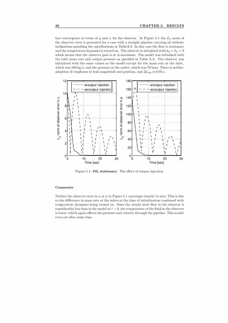
fast convergence in terms of p and u for the observer. In Figure 5.1 the L2 norm of the observer error is presented for a case with a straight pipeline carrying oil without
inclinations matching the specifications in TableA.3. In this case the flow is stationaryand the temperature dynamics is turned on. The observer is initialized with k0 = kL = 0which means that the observer gain is at is maximum. The model was initialized withthe inlet mass rate and output pressure as specified in Table A.3. The observer wasinitialized with the same values as the model except for the mass rate at the inlet,which was 100 kg/s, and the pressure at the outlet, which was 70 bara. There is neitheradaption of roughness or leak magnitude and position, and ∆tobs is 0.05 s.
0 10 20 300
2
4
6
8
10
12
Time [sec]
L 2 n o r m o
f o b s e r v e r e r r o r i n u
w/output injection
wo/output injection
0 10 20 300
20
40
60
80
100
120
140
160
180
Time [sec]
L 2 n o r m o
f o b s e r v e r e r r o r i n p
w/output injection
wo/output injection
Figure 5.1: Oil, stationary. The effect of output injection.
Comments
Neither the observer error in u or p in Figure 5.1 converges exactly to zero. This is dueto the difference in mass rate at the inlets at the time of initialization combined withtemperature dynamics being turned on. Since the steady state flow in the observer isconsiderably less than in the model at t = 0, the temperature of the fluid in the observeris lower, which again affects the pressure and velocity through the pipeline. This wouldeven out after some time.
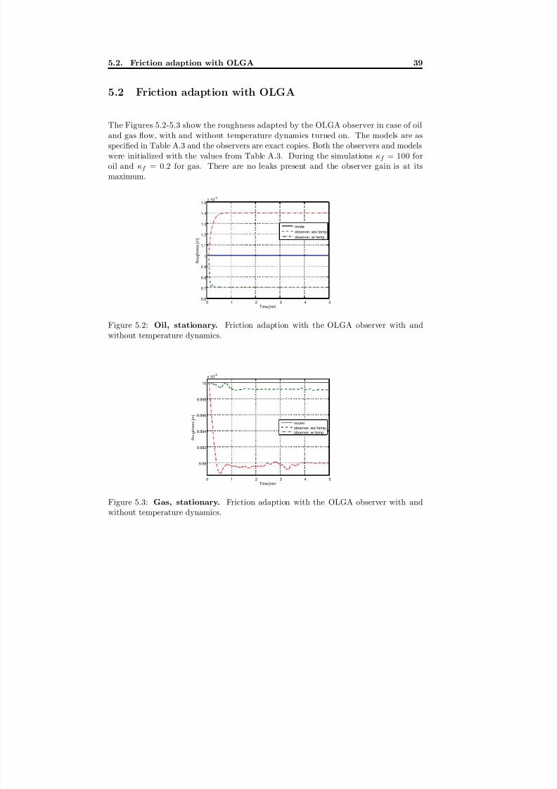
8/18/2019 Advanced Leak Detection using a Nonlinear Observer and OLGA
http://slidepdf.com/reader/full/advanced-leak-detection-using-a-nonlinear-observer-and-olga 47/131
5.2. Friction adaption with OLGA 39
5.2 Friction adaption with OLGA
The Figures 5.2-5.3 show the roughness adapted by the OLGA observer in case of oiland gas flow, with and without temperature dynamics turned on. The models are asspecified in Table A.3 and the observers are exact copies. Both the observers and modelswere initialized with the values from Table A.3. During the simulations κf = 100 foroil and κf = 0.2 for gas. There are no leaks present and the observer gain is at itsmaximum.
0 1 2 3 4 50.6
0.7
0.8
0.9
1
1.1
1.2
1.3
1.4
1.5x 10
−5
Time [min]
R o u g h n e s s [ m ]
model
observer, wo/ temp.
observer, w/ temp.
Figure 5.2: Oil, stationary. Friction adaption with the OLGA observer with and
without temperature dynamics.
0 1 2 3 4 5
9.99
9.992
9.994
9.996
9.998
10
x 10−6
Time [min]
R o u g h n e s s [ m ]
model
observer, wo/ temp.observer, w/ temp.
Figure 5.3: Gas, stationary. Friction adaption with the OLGA observer with andwithout temperature dynamics.
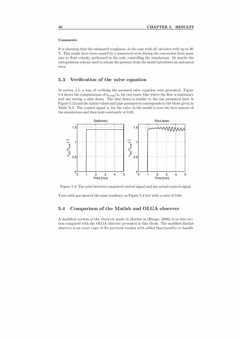
8/18/2019 Advanced Leak Detection using a Nonlinear Observer and OLGA
http://slidepdf.com/reader/full/advanced-leak-detection-using-a-nonlinear-observer-and-olga 48/131
40 CHAPTER 5. RESULTS
Comments
It is alarming that the estimated roughness, in the case with oil, deviates with up to 40%. This might have been caused by a numerical error during the conversion from massrate to fluid velocity performed in the code controlling the simulations. Or maybe theextrapolation scheme used to obtain the pressure from the model introduces an unwantederror.
5.3 Verification of the valve equation
In section 4.5, a way of verifying the assumed valve equation were presented. Figure5.4 shows the computations of u
s,exp/u
s for two cases. One where the flow is stationary
and one during a shut down. The shut down is similar to the one presented later inFigure 5.13 and the initial values and pipe parameters corresponds to the those given inTable A.3. The control signal us for the valve in the model is zero the first minute of the simulations and then held constantly at 0.02.
0 1 2 3 4 50
0.5
1
1.5
Stationary
u o b s
/ u m o d
[ − ]
Time [min]0 1 2 3 4 5
0
0.5
1
1.5
Shut down
u o b s
/ u m o d
[ − ]
Time [min]
Figure 5.4: The ratio between computed control signal and the actual control signal.
Tests with gas showed the same tendency as Figure 5.4 but with a ratio of 0.04.
5.4 Comparison of the Matlab and OLGA observer
A modified version of the observer made in Matlab in (Hauge, 2006) is in this sec-tion compared with the OLGA observer presented in this thesis. The modified Matlabobserver is an exact copy of the previous version with added functionality to handle
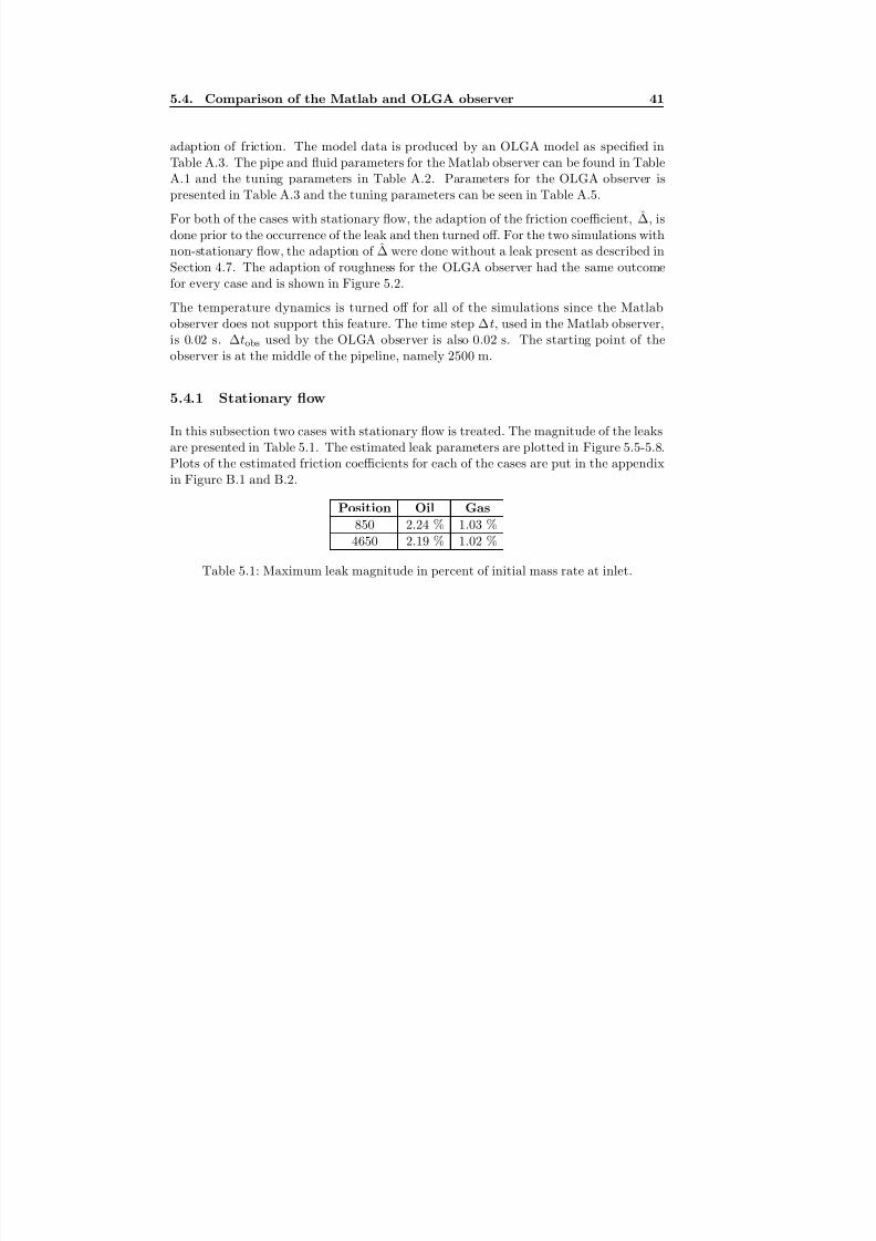
8/18/2019 Advanced Leak Detection using a Nonlinear Observer and OLGA
http://slidepdf.com/reader/full/advanced-leak-detection-using-a-nonlinear-observer-and-olga 49/131
5.4. Comparison of the Matlab and OLGA observer 41
adaption of friction. The model data is produced by an OLGA model as specified inTable A.3. The pipe and fluid parameters for the Matlab observer can be found in Table
A.1 and the tuning parameters in Table A.2. Parameters for the OLGA observer ispresented in Table A.3 and the tuning parameters can be seen in Table A.5.
For both of the cases with stationary flow, the adaption of the friction coefficient, ∆, isdone prior to the occurrence of the leak and then turned off. For the two simulations withnon-stationary flow, the adaption of ∆ were done without a leak present as described inSection 4.7. The adaption of roughness for the OLGA observer had the same outcomefor every case and is shown in Figure 5.2.
The temperature dynamics is turned off for all of the simulations since the Matlabobserver does not support this feature. The time step ∆t, used in the Matlab observer,is 0.02 s. ∆tobs used by the OLGA observer is also 0.02 s. The starting point of the
observer is at the middle of the pipeline, namely 2500 m.
5.4.1 Stationary flow
In this subsection two cases with stationary flow is treated. The magnitude of the leaksare presented in Table 5.1. The estimated leak parameters are plotted in Figure 5.5-5.8.Plots of the estimated friction coefficients for each of the cases are put in the appendixin Figure B.1 and B.2.
Position Oil Gas
850 2.24 % 1.03 %4650 2.19 % 1.02 %
Table 5.1: Maximum leak magnitude in percent of initial mass rate at inlet.
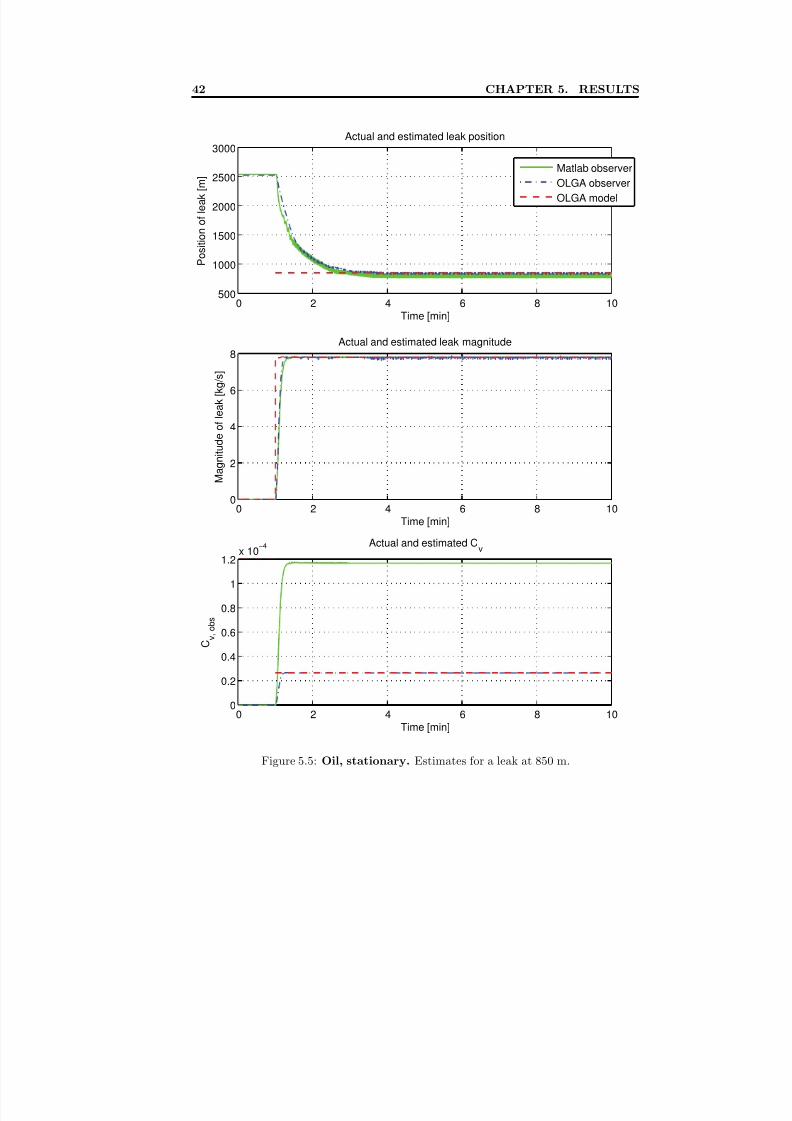
8/18/2019 Advanced Leak Detection using a Nonlinear Observer and OLGA
http://slidepdf.com/reader/full/advanced-leak-detection-using-a-nonlinear-observer-and-olga 50/131
42 CHAPTER 5. RESULTS
0 2 4 6 8 10500
1000
1500
2000
2500
3000Actual and estimated leak position
Time [min]
P o s i t i o n o f l e a k [ m ]
Matlab observer
OLGA observer
OLGA model
0 2 4 6 8 100
2
4
6
8Actual and estimated leak magnitude
M
a g n i t u d e o f l e a k [ k g / s ]
Time [min]
0 2 4 6 8 100
0.2
0.4
0.6
0.8
1
1.2x 10
−4 Actual and estimated Cv
C v , o b s
Time [min]
Figure 5.5: Oil, stationary. Estimates for a leak at 850 m.
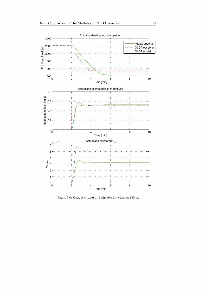
8/18/2019 Advanced Leak Detection using a Nonlinear Observer and OLGA
http://slidepdf.com/reader/full/advanced-leak-detection-using-a-nonlinear-observer-and-olga 51/131
5.4. Comparison of the Matlab and OLGA observer 43
0 2 4 6 8 10500
1000
1500
2000
2500
3000Actual and estimated leak position
Time [min]
P o s i t i o n o f l e a k [ m ]
Matlab observer
OLGA observer
OLGA model
0 2 4 6 8 100
0.2
0.4
0.6
0.8Actual and estimated leak magnitude
M
a g n i t u d e o f l e a k [ k g / s ]
Time [min]
0 2 4 6 8 100
1
2
3
4
5
6x 10
−5 Actual and estimated Cv
C v , o b s
Time [min]
Figure 5.6: Gas, stationary. Estimates for a leak at 850 m.
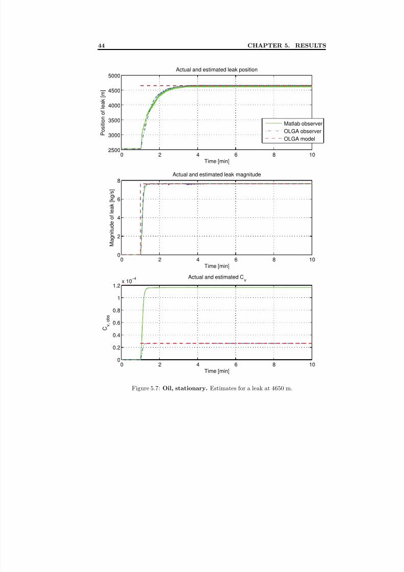
8/18/2019 Advanced Leak Detection using a Nonlinear Observer and OLGA
http://slidepdf.com/reader/full/advanced-leak-detection-using-a-nonlinear-observer-and-olga 52/131
44 CHAPTER 5. RESULTS
0 2 4 6 8 102500
3000
3500
4000
4500
5000Actual and estimated leak position
Time [min]
P o s i t i o n o f l e a k [ m ]
Matlab observer
OLGA observer
OLGA model
0 2 4 6 8 100
2
4
6
8Actual and estimated leak magnitude
M
a g n i t u d e o f l e a k [ k g / s ]
Time [min]
0 2 4 6 8 100
0.2
0.4
0.6
0.8
1
1.2x 10
−4 Actual and estimated Cv
C v , o b s
Time [min]
Figure 5.7: Oil, stationary. Estimates for a leak at 4650 m.
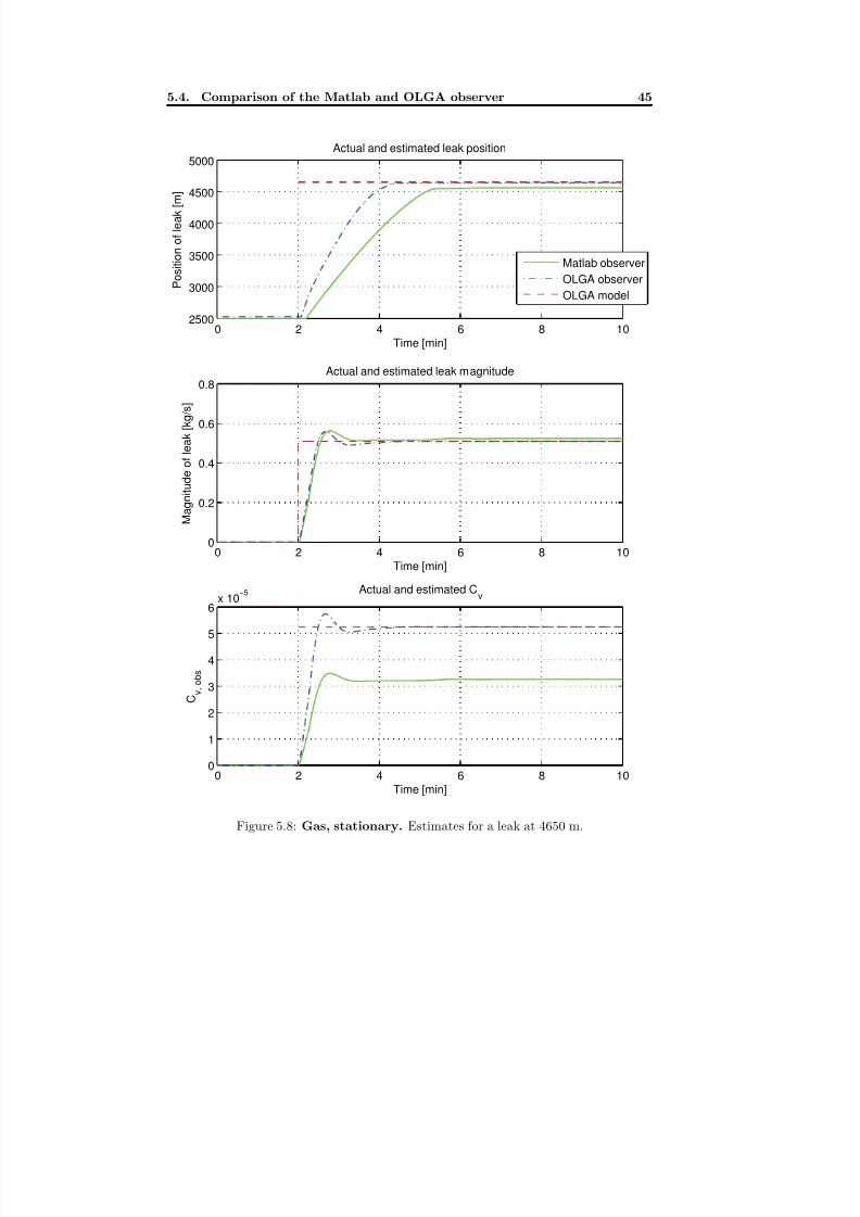
8/18/2019 Advanced Leak Detection using a Nonlinear Observer and OLGA
http://slidepdf.com/reader/full/advanced-leak-detection-using-a-nonlinear-observer-and-olga 53/131
5.4. Comparison of the Matlab and OLGA observer 45
0 2 4 6 8 102500
3000
3500
4000
4500
5000Actual and estimated leak position
Time [min]
P o s i t i o n o f l e a k [ m ]
Matlab observer
OLGA observer
OLGA model
0 2 4 6 8 100
0.2
0.4
0.6
0.8Actual and estimated leak magnitude
M
a g n i t u d e o f l e a k [ k g / s ]
Time [min]
0 2 4 6 8 100
1
2
3
4
5
6x 10
−5 Actual and estimated Cv
C v , o b s
Time [min]
Figure 5.8: Gas, stationary. Estimates for a leak at 4650 m.
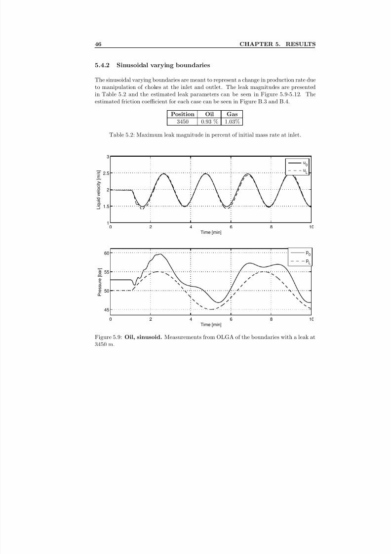
8/18/2019 Advanced Leak Detection using a Nonlinear Observer and OLGA
http://slidepdf.com/reader/full/advanced-leak-detection-using-a-nonlinear-observer-and-olga 54/131
46 CHAPTER 5. RESULTS
5.4.2 Sinusoidal varying boundaries
The sinusoidal varying boundaries are meant to represent a change in production rate dueto manipulation of chokes at the inlet and outlet. The leak magnitudes are presentedin Table 5.2 and the estimated leak parameters can be seen in Figure 5.9-5.12. Theestimated friction coefficient for each case can be seen in Figure B.3 and B.4.
Position Oil Gas
3450 0.93 % 1.03%
Table 5.2: Maximum leak magnitude in percent of initial mass rate at inlet.
0 2 4 6 8 101
1.5
2
2.5
3
Time [min]
L i q u i d v e l o c i t y [ m / s ]
u0
uL
0 2 4 6 8 10
45
50
55
60
Time [min]
P r e s s u r e [ b a r ]
p0
pL
Figure 5.9: Oil, sinusoid. Measurements from OLGA of the boundaries with a leak at3450 m.
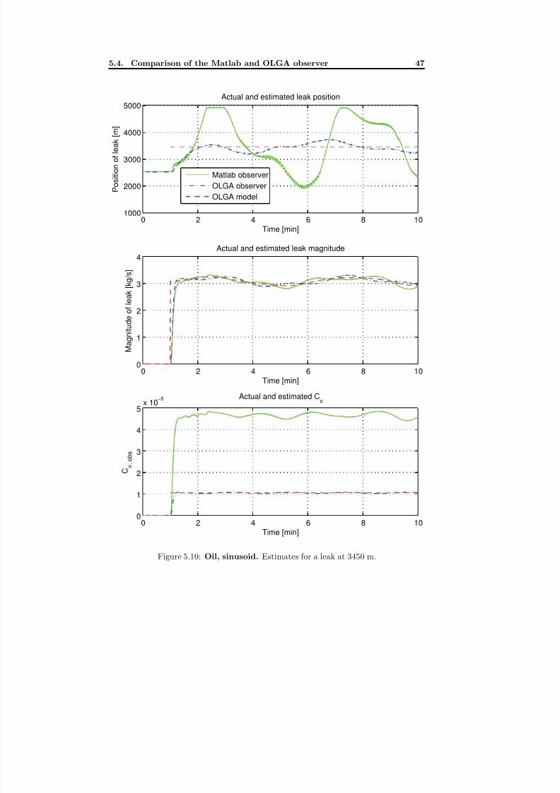
8/18/2019 Advanced Leak Detection using a Nonlinear Observer and OLGA
http://slidepdf.com/reader/full/advanced-leak-detection-using-a-nonlinear-observer-and-olga 55/131
5.4. Comparison of the Matlab and OLGA observer 47
0 2 4 6 8 101000
2000
3000
4000
5000Actual and estimated leak position
Time [min]
P o s i t i o n o f l e a k [ m ]
Matlab observer
OLGA observer
OLGA model
0 2 4 6 8 100
1
2
3
4Actual and estimated leak magnitude
M a g
n i t u d e o f l e a k [ k g / s ]
Time [min]
0 2 4 6 8 100
1
2
3
4
5x 10
−5 Actual and estimated Cv
C v , o b s
Time [min]
Figure 5.10: Oil, sinusoid. Estimates for a leak at 3450 m.
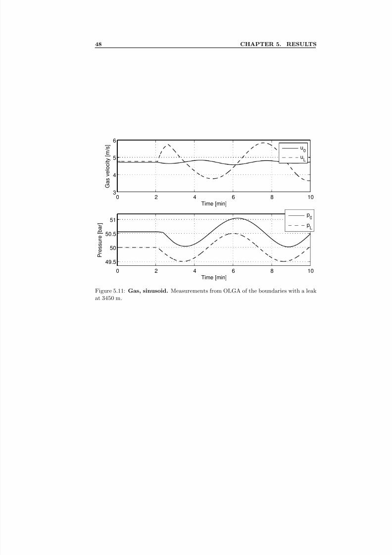
8/18/2019 Advanced Leak Detection using a Nonlinear Observer and OLGA
http://slidepdf.com/reader/full/advanced-leak-detection-using-a-nonlinear-observer-and-olga 56/131
48 CHAPTER 5. RESULTS
0 2 4 6 8 103
4
5
6
Time [min]
G a s v e l o c i t y
[ m / s ]
u0
uL
0 2 4 6 8 10
49.5
50
50.5
51
Time [min]
P r e s s u r e
[ b a r ]
p0
pL
Figure 5.11: Gas, sinusoid. Measurements from OLGA of the boundaries with a leakat 3450 m.
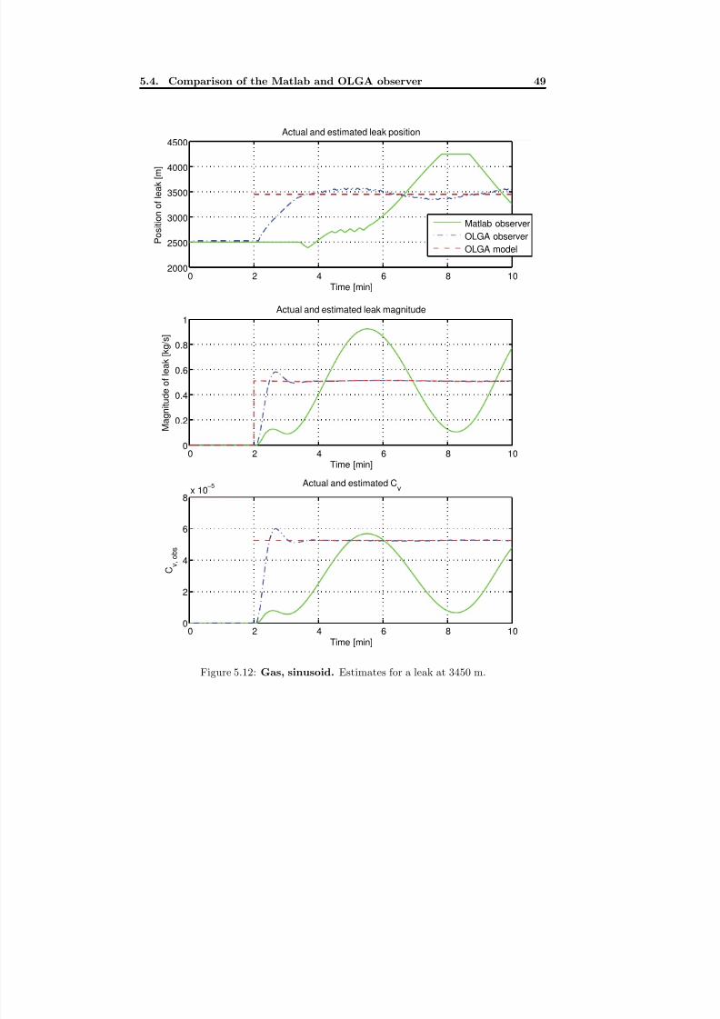
8/18/2019 Advanced Leak Detection using a Nonlinear Observer and OLGA
http://slidepdf.com/reader/full/advanced-leak-detection-using-a-nonlinear-observer-and-olga 57/131
5.4. Comparison of the Matlab and OLGA observer 49
0 2 4 6 8 102000
2500
3000
3500
4000
4500
Actual and estimated leak position
Time [min]
P o s i t i o n o f l e a k [ m ]
Matlab observer
OLGA observer
OLGA model
0 2 4 6 8 100
0.2
0.4
0.6
0.8
1Actual and estimated leak magnitude
M a g n i t u d e o f l e a k [ k g / s ]
Time [min]
0 2 4 6 8 100
2
4
6
8x 10
−5 Actual and estimated Cv
C v , o b s
Time [min]
Figure 5.12: Gas, sinusoid. Estimates for a leak at 3450 m.
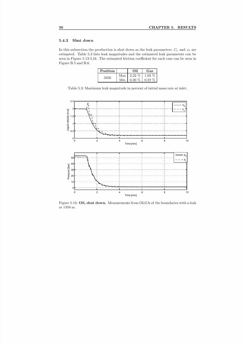
8/18/2019 Advanced Leak Detection using a Nonlinear Observer and OLGA
http://slidepdf.com/reader/full/advanced-leak-detection-using-a-nonlinear-observer-and-olga 58/131
50 CHAPTER 5. RESULTS
5.4.3 Shut down
In this subsection the production is shut down as the leak parameters C v and xl areestimated. Table 5.3 lists leak magnitudes and the estimated leak parameters can beseen in Figure 5.13-5.16. The estimated friction coefficient for each case can be seen inFigure B.5 and B.6.
Position Oil Gas
3450 Max 2.22 % 1.03 %
Min 0.20 % 0.22 %
Table 5.3: Maximum leak magnitude in percent of initial mass rate at inlet.
0 2 4 6 8 100
0.5
1
1.5
2
2.5
Time [min]
L i q u i d v e l o c i t y [ m / s ]
u0
uL
0 2 4 6 8 10
0
10
20
30
40
50
Time [min]
P r e s s u r e [ b a r ]
p0
pL
Figure 5.13: Oil, shut down. Measurements from OLGA of the boundaries with a leakat 1350 m.
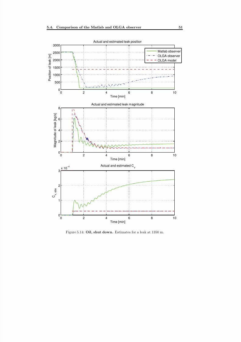
8/18/2019 Advanced Leak Detection using a Nonlinear Observer and OLGA
http://slidepdf.com/reader/full/advanced-leak-detection-using-a-nonlinear-observer-and-olga 59/131
5.4. Comparison of the Matlab and OLGA observer 51
0 2 4 6 8 100
500
1000
1500
2000
2500
3000Actual and estimated leak position
Time [min]
P o s i t i o n o f l e a k [ m ]
Matlab observer
OLGA observer
OLGA model
0 2 4 6 8 100
2
4
6
8Actual and estimated leak magnitude
M
a g n i t u d e o f l e a k [ k g / s ]
Time [min]
0 2 4 6 8 100
1
2
3x 10
−4 Actual and estimated Cv
C v , o b s
Time [min]
Figure 5.14: Oil, shut down. Estimates for a leak at 1350 m.
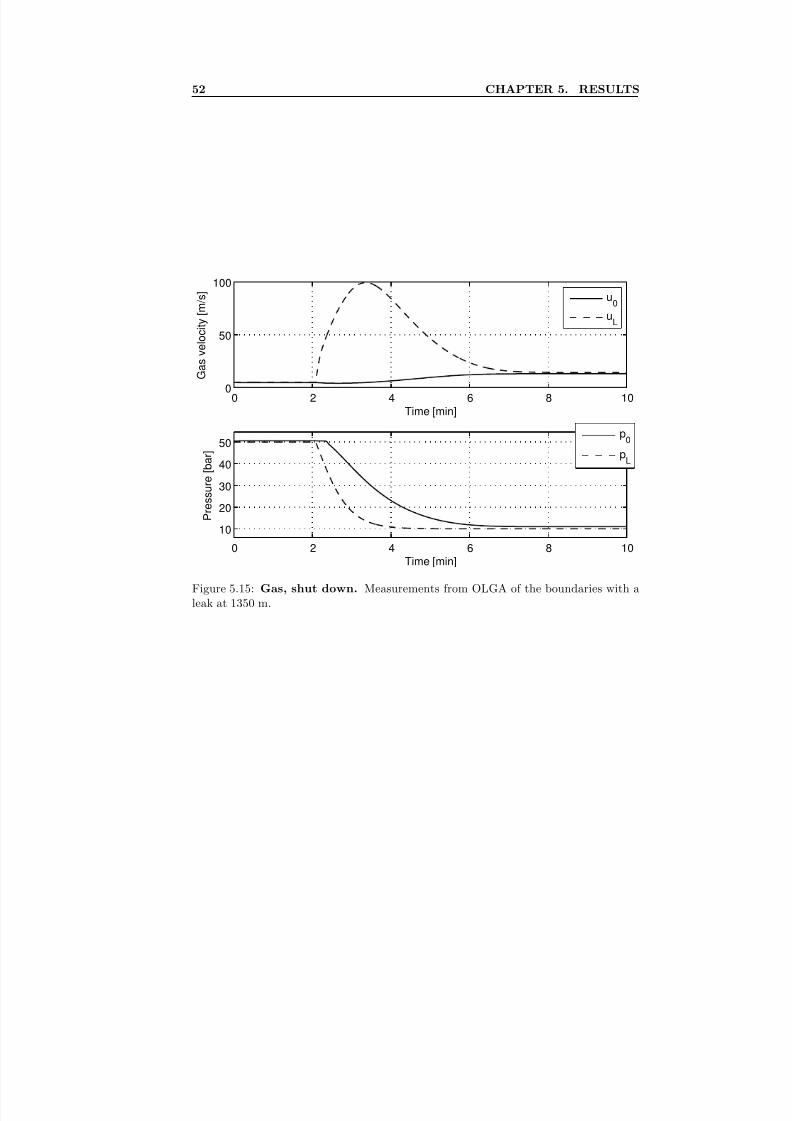
8/18/2019 Advanced Leak Detection using a Nonlinear Observer and OLGA
http://slidepdf.com/reader/full/advanced-leak-detection-using-a-nonlinear-observer-and-olga 60/131
52 CHAPTER 5. RESULTS
0 2 4 6 8 100
50
100
Time [min]
G a s v e l o c i t y
[ m / s ]
u0
uL
0 2 4 6 8 10
10
20
30
40
50
Time [min]
P r e s s u r e
[ b a r ]
p0
pL
Figure 5.15: Gas, shut down. Measurements from OLGA of the boundaries with aleak at 1350 m.
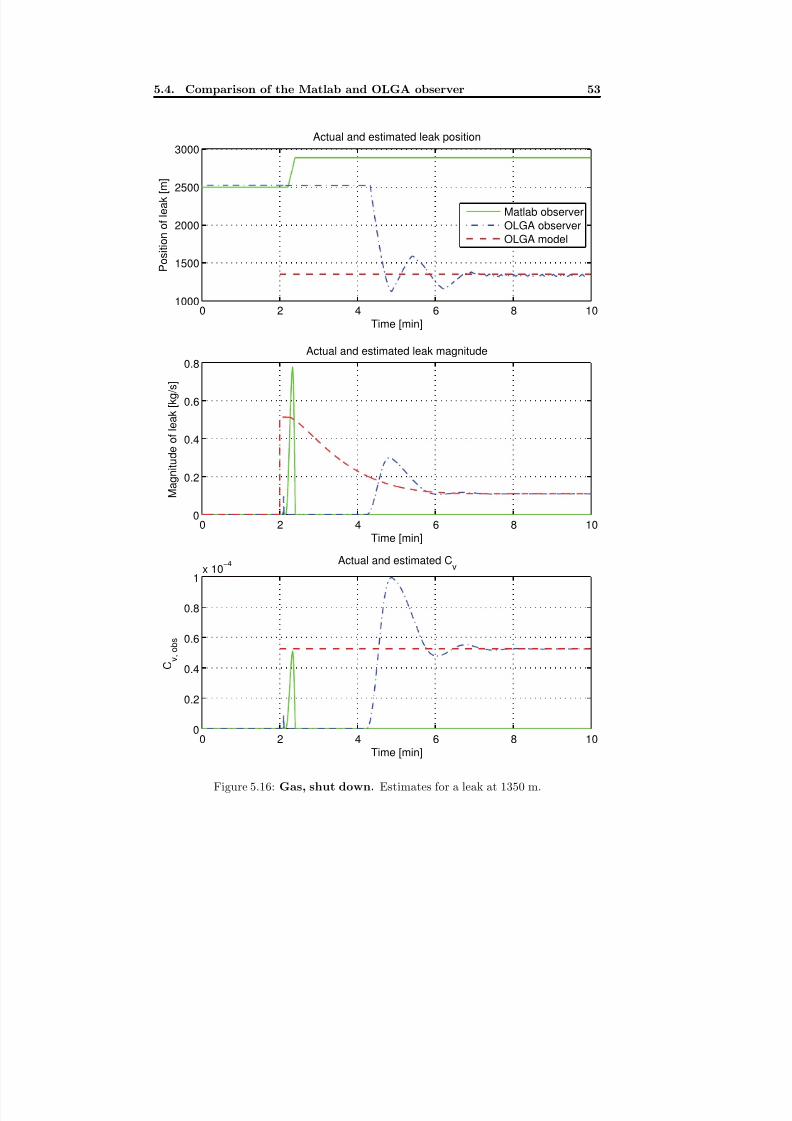
8/18/2019 Advanced Leak Detection using a Nonlinear Observer and OLGA
http://slidepdf.com/reader/full/advanced-leak-detection-using-a-nonlinear-observer-and-olga 61/131
5.4. Comparison of the Matlab and OLGA observer 53
0 2 4 6 8 101000
1500
2000
2500
3000Actual and estimated leak position
Time [min]
P o s i t i o n o f l e a k [ m ]
Matlab observer
OLGA observer
OLGA model
0 2 4 6 8 100
0.2
0.4
0.6
0.8Actual and estimated leak magnitude
M a g
n i t u d e o f l e a k [ k g / s ]
Time [min]
0 2 4 6 8 100
0.2
0.4
0.6
0.8
1x 10
−4 Actual and estimated Cv
C v , o b s
Time [min]
Figure 5.16: Gas, shut down. Estimates for a leak at 1350 m.
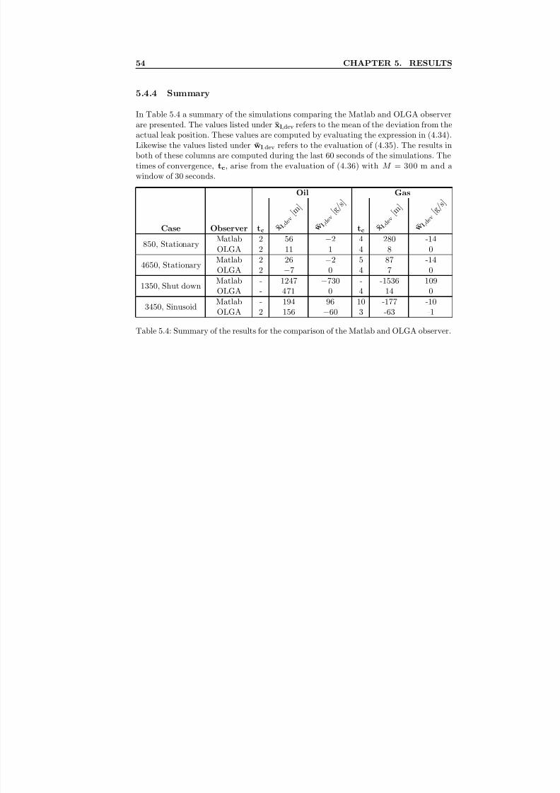
8/18/2019 Advanced Leak Detection using a Nonlinear Observer and OLGA
http://slidepdf.com/reader/full/advanced-leak-detection-using-a-nonlinear-observer-and-olga 62/131
54 CHAPTER 5. RESULTS
5.4.4 Summary
In Table 5.4 a summary of the simulations comparing the Matlab and OLGA observerare presented. The values listed under xl,dev refers to the mean of the deviation from theactual leak position. These values are computed by evaluating the expression in (4.34).Likewise the values listed under wl,dev refers to the evaluation of (4.35). The results inboth of these columns are computed during the last 60 seconds of the simulations. Thetimes of convergence, tc, arise from the evaluation of (4.36) with M = 300 m and awindow of 30 seconds.
Oil Gas
Case Observer tc ¯ x l, d e v [ m
]
¯ w l,
d e v [ g
/ s ]
tc ¯ x l, d e v [ m
]
¯ w l,
d e v [ g
/ s ]
850, Stationary Matlab 2 56 −2 4 280 -14
OLGA 2 11 1 4 8 0
4650, Stationary Matlab 2 26 −2 5 87 -14
OLGA 2 −7 0 4 7 0
1350, Shut down Matlab - 1247 −730 - -1536 109
OLGA - 471 0 4 14 0
3450, Sinusoid Matlab - 194 96 10 -177 -10
OLGA 2 156 −60 3 -63 -1
Table 5.4: Summary of the results for the comparison of the Matlab and OLGA observer.
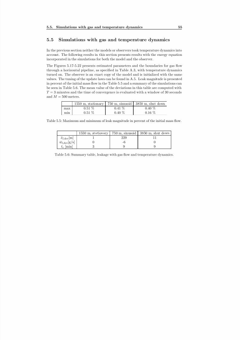
8/18/2019 Advanced Leak Detection using a Nonlinear Observer and OLGA
http://slidepdf.com/reader/full/advanced-leak-detection-using-a-nonlinear-observer-and-olga 63/131
5.5. Simulations with gas and temperature dynamics 55
5.5 Simulations with gas and temperature dynamics
In the previous section neither the models or observers took temperature dynamics intoaccount. The following results in this section presents results with the energy equationincorporated in the simulations for both the model and the observer.
The Figures 5.17-5.22 presents estimated parameters and the boundaries for gas flowthrough a horizontal pipeline, as specified in Table A.3, with temperature dynamicsturned on. The observer is an exact copy of the model and is initialized with the samevalues. The tuning of the update laws can be found in A.5. Leak magnitude is presentedin percent of the initial mass flow in the Table 5.5 and a summary of the simulations canbe seen in Table 5.6. The mean value of the deviations in this table are computed withT = 3 minutes and the time of convergence is evaluated with a window of 30 seconds
and M = 500 meters.
1550 m, stationary 750 m, sinusoid 3850 m, shut down
max 0.51 % 0.41 % 0.40 %min 0.51 % 0.40 % 0.16 %
Table 5.5: Maximum and minimum of leak magnitude in percent of the initial mass flow.
1550 m, stationary 750 m, sinusoid 3850 m, shut down
xl,dev[m] 1 229 11wl,dev[g/s] 0 -6 0
tc [min] 3 9 9
Table 5.6: Summary table, leakage with gas flow and temperature dynamics.
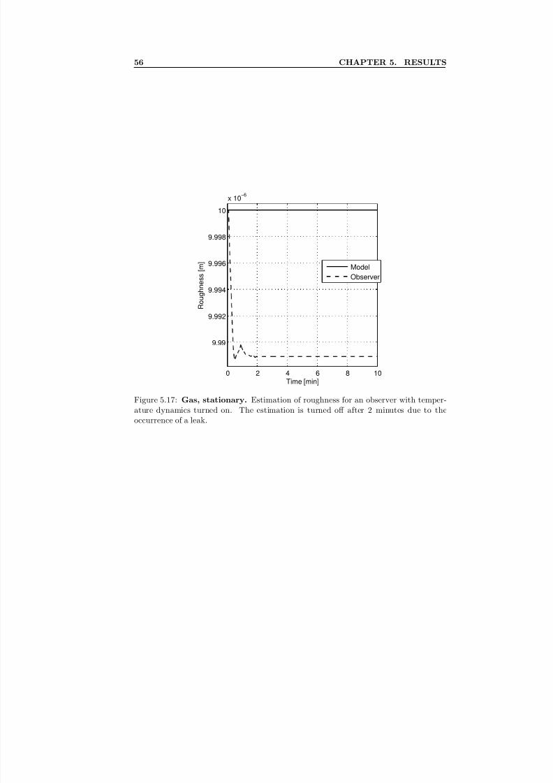
8/18/2019 Advanced Leak Detection using a Nonlinear Observer and OLGA
http://slidepdf.com/reader/full/advanced-leak-detection-using-a-nonlinear-observer-and-olga 64/131
56 CHAPTER 5. RESULTS
0 2 4 6 8 10
9.99
9.992
9.994
9.996
9.998
10
x 10−6
Time [min]
R o u g h n e s s [ m ]
Model
Observer
Figure 5.17: Gas, stationary. Estimation of roughness for an observer with temper-ature dynamics turned on. The estimation is turned off after 2 minutes due to theoccurrence of a leak.
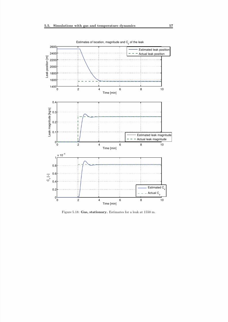
8/18/2019 Advanced Leak Detection using a Nonlinear Observer and OLGA
http://slidepdf.com/reader/full/advanced-leak-detection-using-a-nonlinear-observer-and-olga 65/131
5.5. Simulations with gas and temperature dynamics 57
0 2 4 6 8 101400
1600
1800
2000
2200
2400
2600
Estimates of location, magnitude and Cv of the leak
Time [min]
L e a k p o s i t i o n [ m ]
Estimated leak position
Actual leak position
0 2 4 6 8 100
0.1
0.2
0.3
0.4
Time [min]
L e a k m a g n i t u d e [ k g / s ]
Estimated leak magnitude
Actual leak magnitude
0 2 4 6 8 100
0.2
0.4
0.6
0.8
1x 10
−4
Time [min]
C v
[ − ]
Estimated Cv
Actual Cv
Figure 5.18: Gas, stationary. Estimates for a leak at 1550 m.
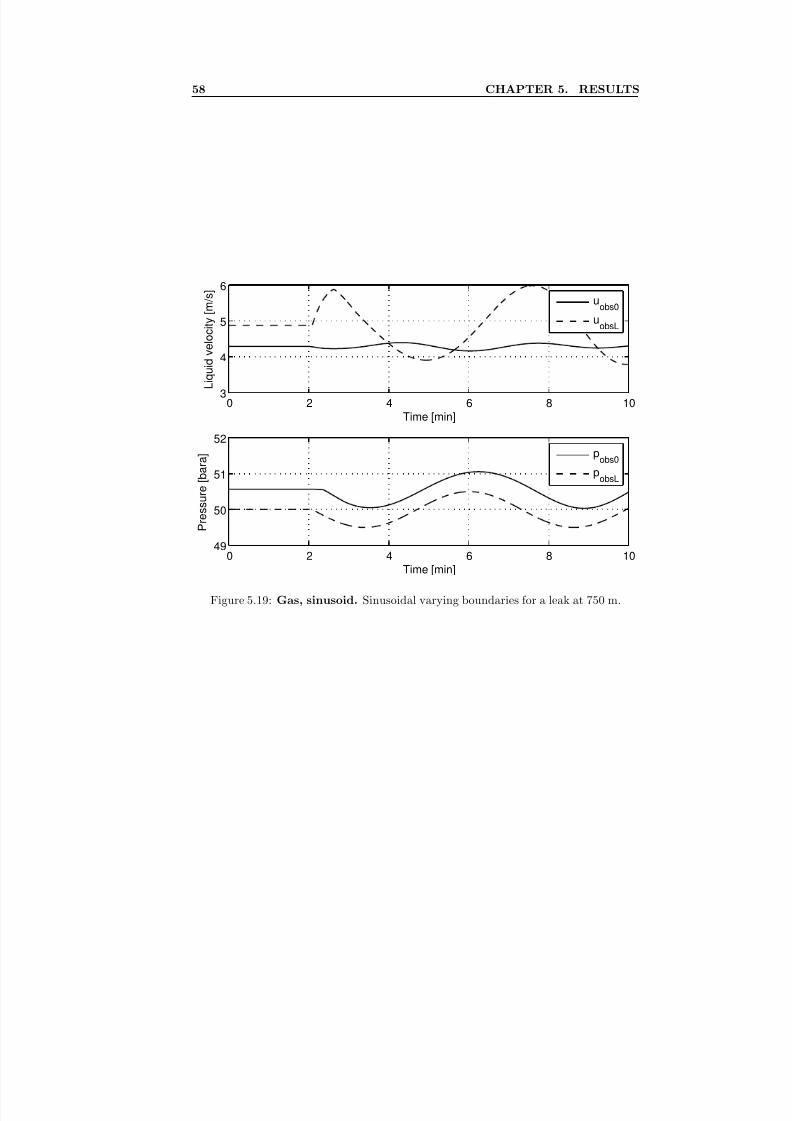
8/18/2019 Advanced Leak Detection using a Nonlinear Observer and OLGA
http://slidepdf.com/reader/full/advanced-leak-detection-using-a-nonlinear-observer-and-olga 66/131
58 CHAPTER 5. RESULTS
0 2 4 6 8 103
4
5
6
Time [min]
L i q u i d v e l o c i t y
[ m / s ]
uobs0
uobsL
0 2 4 6 8 1049
50
51
52
Time [min]
P r e s s u r e [ b
a r a ] p
obs0
pobsL
Figure 5.19: Gas, sinusoid. Sinusoidal varying boundaries for a leak at 750 m.
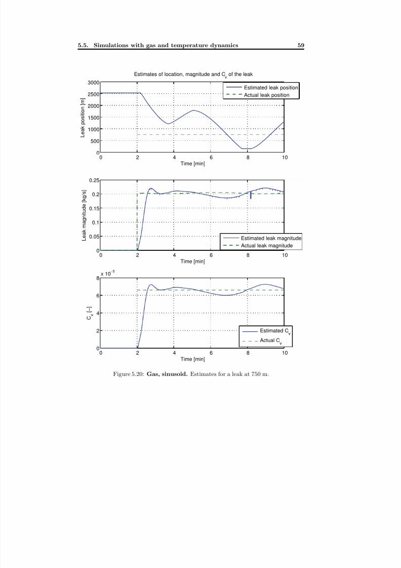
8/18/2019 Advanced Leak Detection using a Nonlinear Observer and OLGA
http://slidepdf.com/reader/full/advanced-leak-detection-using-a-nonlinear-observer-and-olga 67/131
5.5. Simulations with gas and temperature dynamics 59
0 2 4 6 8 100
500
1000
1500
2000
2500
3000
Estimates of location, magnitude and Cv of the leak
Time [min]
L e a k p o s i t i o n [ m ]
Estimated leak position
Actual leak position
0 2 4 6 8 100
0.05
0.1
0.15
0.2
0.25
Time [min]
L e a k m a g n i t u d e [ k g / s ]
Estimated leak magnitude
Actual leak magnitude
0 2 4 6 8 100
2
4
6
8x 10
−5
Time [min]
C v
[ − ]
Estimated Cv
Actual Cv
Figure 5.20: Gas, sinusoid. Estimates for a leak at 750 m.
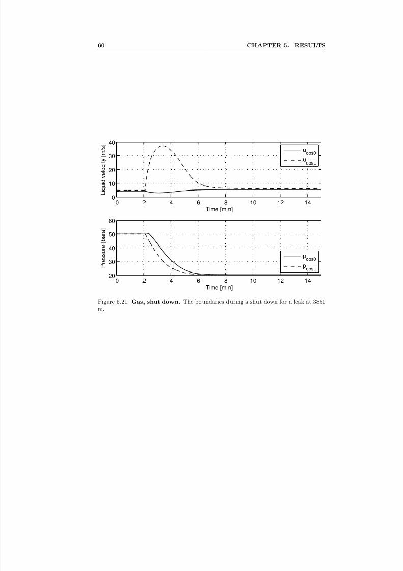
8/18/2019 Advanced Leak Detection using a Nonlinear Observer and OLGA
http://slidepdf.com/reader/full/advanced-leak-detection-using-a-nonlinear-observer-and-olga 68/131
60 CHAPTER 5. RESULTS
0 2 4 6 8 10 12 140
10
20
30
40
Time [min]
L i q u i d v e l o c i t y [ m / s ]
uobs0
uobsL
0 2 4 6 8 10 12 1420
30
40
50
60
Time [min]
P r e s s u r e [ b a r a ]
pobs0
pobsL
Figure 5.21: Gas, shut down. The boundaries during a shut down for a leak at 3850m.
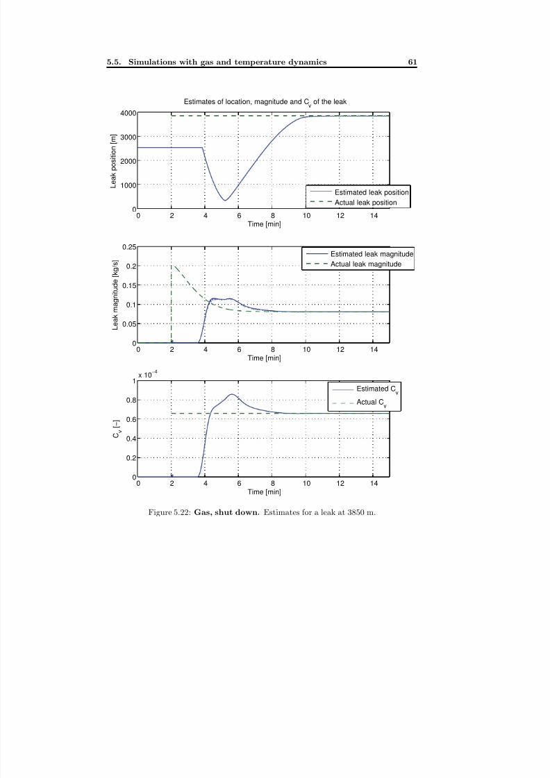
8/18/2019 Advanced Leak Detection using a Nonlinear Observer and OLGA
http://slidepdf.com/reader/full/advanced-leak-detection-using-a-nonlinear-observer-and-olga 69/131
5.5. Simulations with gas and temperature dynamics 61
0 2 4 6 8 10 12 140
1000
2000
3000
4000
Estimates of location, magnitude and Cv of the leak
Time [min]
L e a k p o s i t i o n [ m ]
Estimated leak position
Actual leak position
0 2 4 6 8 10 12 140
0.05
0.1
0.15
0.2
0.25
Time [min]
L e a k m a g n i t u d e [ k g / s ]
Estimated leak magnitude
Actual leak magnitude
0 2 4 6 8 10 12 140
0.2
0.4
0.6
0.8
1x 10
−4
Time [min]
C v
[ − ]
Estimated Cv
Actual Cv
Figure 5.22: Gas, shut down. Estimates for a leak at 3850 m.
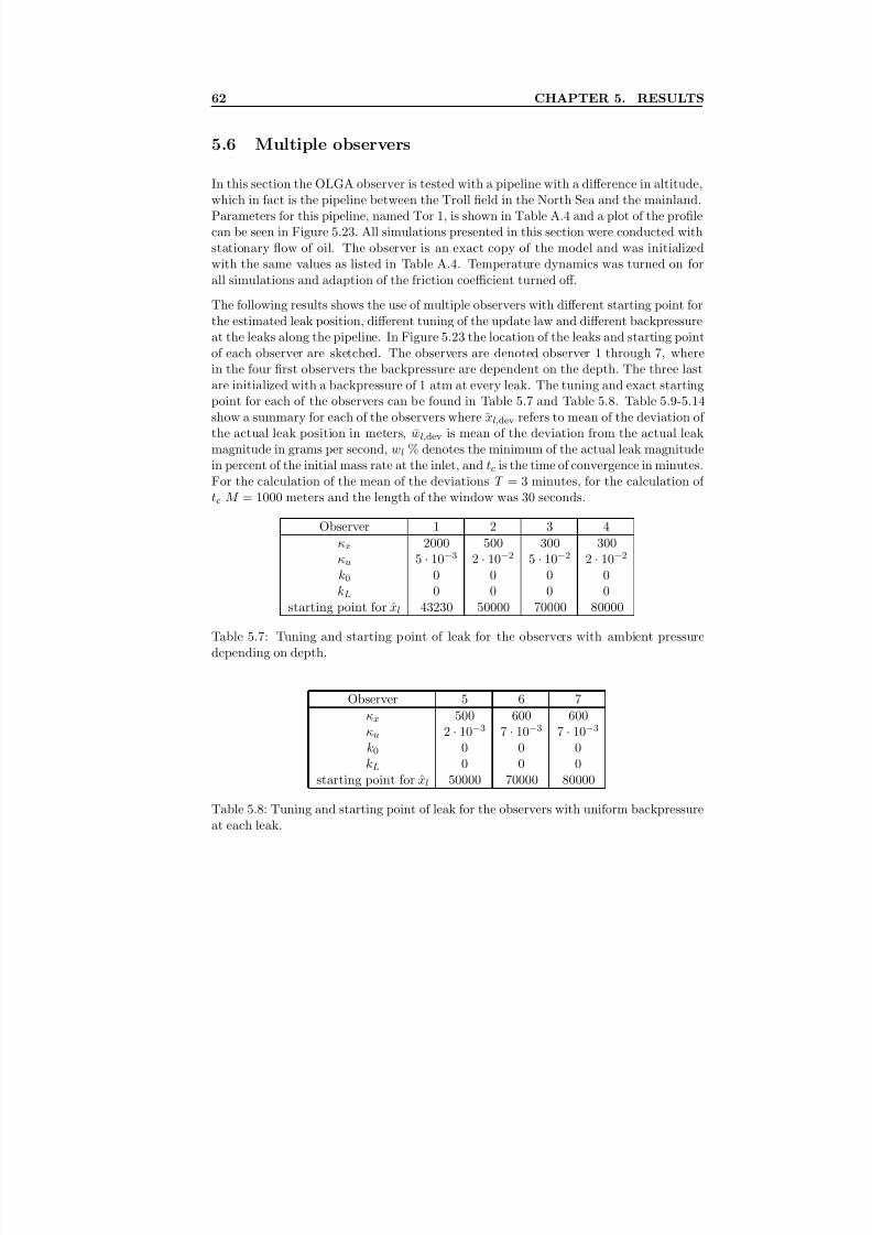
8/18/2019 Advanced Leak Detection using a Nonlinear Observer and OLGA
http://slidepdf.com/reader/full/advanced-leak-detection-using-a-nonlinear-observer-and-olga 70/131
62 CHAPTER 5. RESULTS
5.6 Multiple observers
In this section the OLGA observer is tested with a pipeline with a difference in altitude,which in fact is the pipeline between the Troll field in the North Sea and the mainland.Parameters for this pipeline, named Tor 1, is shown in Table A.4 and a plot of the profilecan be seen in Figure 5.23. All simulations presented in this section were conducted withstationary flow of oil. The observer is an exact copy of the model and was initializedwith the same values as listed in Table A.4. Temperature dynamics was turned on forall simulations and adaption of the friction coefficient turned off.
The following results shows the use of multiple observers with different starting point forthe estimated leak position, different tuning of the update law and different backpressureat the leaks along the pipeline. In Figure 5.23 the location of the leaks and starting point
of each observer are sketched. The observers are denoted observer 1 through 7, wherein the four first observers the backpressure are dependent on the depth. The three lastare initialized with a backpressure of 1 atm at every leak. The tuning and exact startingpoint for each of the observers can be found in Table 5.7 and Table 5.8. Table 5.9-5.14show a summary for each of the observers where xl,dev refers to mean of the deviation of the actual leak position in meters, wl,dev is mean of the deviation from the actual leakmagnitude in grams per second, wl % denotes the minimum of the actual leak magnitudein percent of the initial mass rate at the inlet, and tc is the time of convergence in minutes.For the calculation of the mean of the deviations T = 3 minutes, for the calculation of tc M = 1000 meters and the length of the window was 30 seconds.
Observer 1 2 3 4κx 2000 500 300 300κu 5 · 10−3 2 · 10−2 5 · 10−2 2 · 10−2
k0 0 0 0 0kL 0 0 0 0
starting point for xl 43230 50000 70000 80000
Table 5.7: Tuning and starting point of leak for the observers with ambient pressuredepending on depth.
Observer 5 6 7κx 500 600 600κu 2 · 10−3 7 · 10−3 7 · 10−3
k0 0 0 0kL 0 0 0
starting point for xl 50000 70000 80000
Table 5.8: Tuning and starting point of leak for the observers with uniform backpressureat each leak.
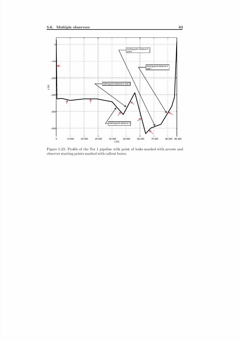
8/18/2019 Advanced Leak Detection using a Nonlinear Observer and OLGA
http://slidepdf.com/reader/full/advanced-leak-detection-using-a-nonlinear-observer-and-olga 71/131
5.6. Multiple observers 63
0 10 000 20 000 30 000 40 000 50 000 60 000 70 000 80 000 86 460
−500
−400
−300
−200
−100
0
x [m]
y [ m ]
starting point observer 1
starting point observer 3and 6
starting point observer 2 and 5
starting point observer 4and 7
Figure 5.23: Profile of the Tor 1 pipeline with point of leaks marked with arrows andobserver starting points marked with callout boxes.
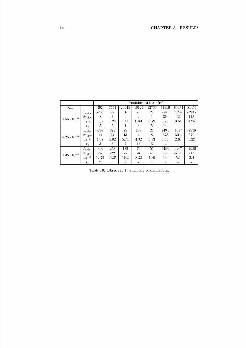
8/18/2019 Advanced Leak Detection using a Nonlinear Observer and OLGA
http://slidepdf.com/reader/full/advanced-leak-detection-using-a-nonlinear-observer-and-olga 72/131
64 CHAPTER 5. RESULTS
Position of leak [m]
Cv 292 7751 23645 46624 52766 61316 66474 81454
1.65 · 10−5
xl,dev -266 27 56 -1 29 -548 3394 -2936wl,dev -8 3 1 2 1 30 -39 113wl % 1.39 1.24 1.11 0.89 0.79 0.73 0.54 0.25
tc 5 5 4 3 5 14 - -
8.25 · 10−5
xl,dev -297 323 75 157 25 2494 4687 -2936wl,dev -41 24 13 4 8 -673 -3014 379wl % 6.68 5.92 5.34 4.32 3.83 3.55 2.63 1.22
tc 3 8 5 15 5 14 - -
1.65 · 10−4xl,dev -309 253 182 79 57 1453 9267 -2936wl,dev -87 -22 -5 -8 -8 -591 -6190 713wl % 12.72 11.25 10.2 8.32 7.39 6.9 5.1 2.4
tc 2 6 5 - 15 14 - -
Table 5.9: Observer 1. Summary of simulations.
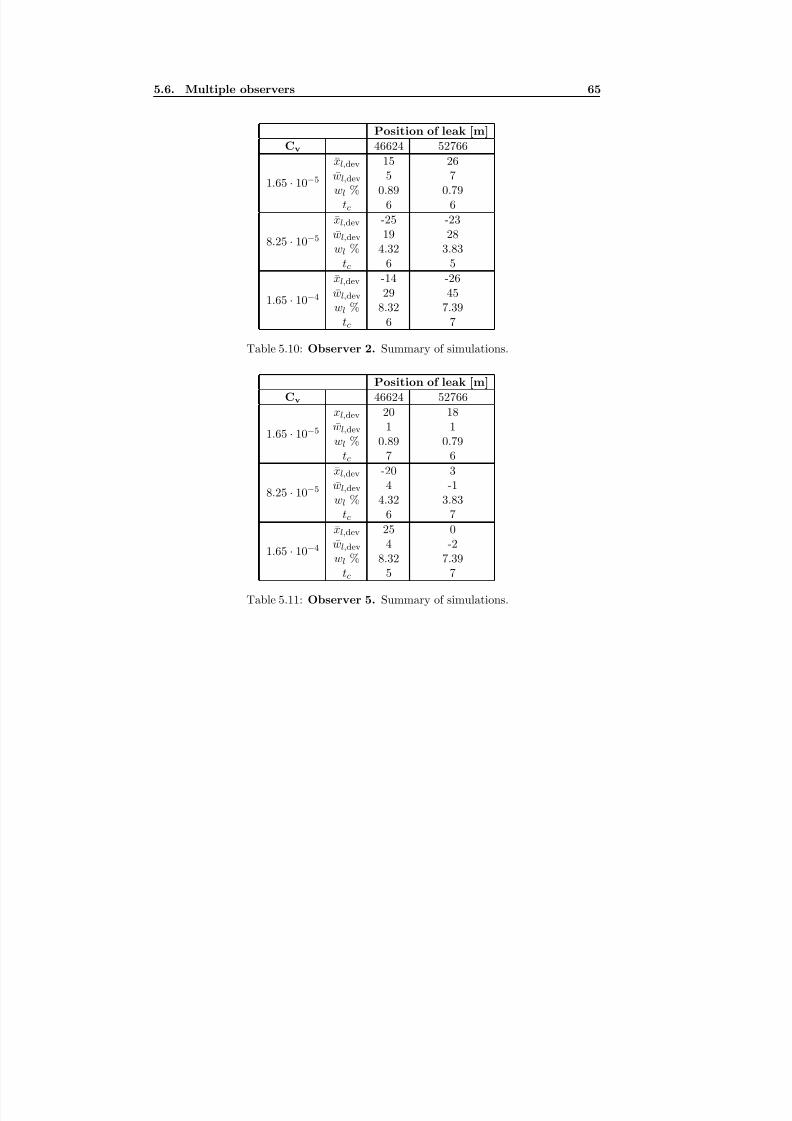
8/18/2019 Advanced Leak Detection using a Nonlinear Observer and OLGA
http://slidepdf.com/reader/full/advanced-leak-detection-using-a-nonlinear-observer-and-olga 73/131
5.6. Multiple observers 65
Position of leak [m]
Cv 46624 52766
1.65 · 10−5xl,dev 15 26wl,dev 5 7wl % 0.89 0.79
tc 6 6
8.25 · 10−5
xl,dev -25 -23wl,dev 19 28wl % 4.32 3.83
tc 6 5
1.65 · 10−4
xl,dev -14 -26wl,dev 29 45wl % 8.32 7.39
tc 6 7
Table 5.10: Observer 2. Summary of simulations.
Position of leak [m]
Cv 46624 52766
1.65 · 10−5
xl,dev 20 18wl,dev 1 1wl % 0.89 0.79
tc 7 6
8.25 · 10−5
xl,dev -20 3wl,dev 4 -1wl % 4.32 3.83
tc 6 7
1.65 · 10−4
xl,dev 25 0wl,dev 4 -2wl % 8.32 7.39
tc 5 7
Table 5.11: Observer 5. Summary of simulations.
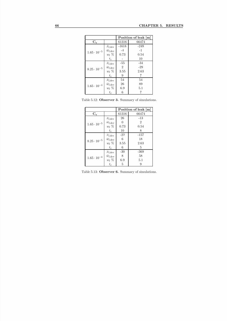
8/18/2019 Advanced Leak Detection using a Nonlinear Observer and OLGA
http://slidepdf.com/reader/full/advanced-leak-detection-using-a-nonlinear-observer-and-olga 74/131
66 CHAPTER 5. RESULTS
Position of leak [m]
Cv 61316 66474
1.65 · 10−5xl,dev -1618 -249wl,dev -4 -1wl % 0.73 0.54
tc - 10
8.25 · 10−5
xl,dev -55 -34wl,dev 2 -29wl % 3.55 2.63
tc 9 7
1.65 · 10−4
xl,dev 54 54wl,dev 26 89wl % 6.9 5.1
tc 6 7
Table 5.12: Observer 3. Summary of simulations.
Position of leak [m]
Cv 61316 66474
1.65 · 10−5
xl,dev 26 -13wl,dev 0 2wl % 0.73 0.54
tc 10 8
8.25 · 10−5
xl,dev -22 -157wl,dev 6 18wl % 3.55 2.63
tc 6 5
1.65 · 10−4
xl,dev -30 -369wl,dev 8 58wl % 6.9 5.1
tc 5 9
Table 5.13: Observer 6. Summary of simulations.
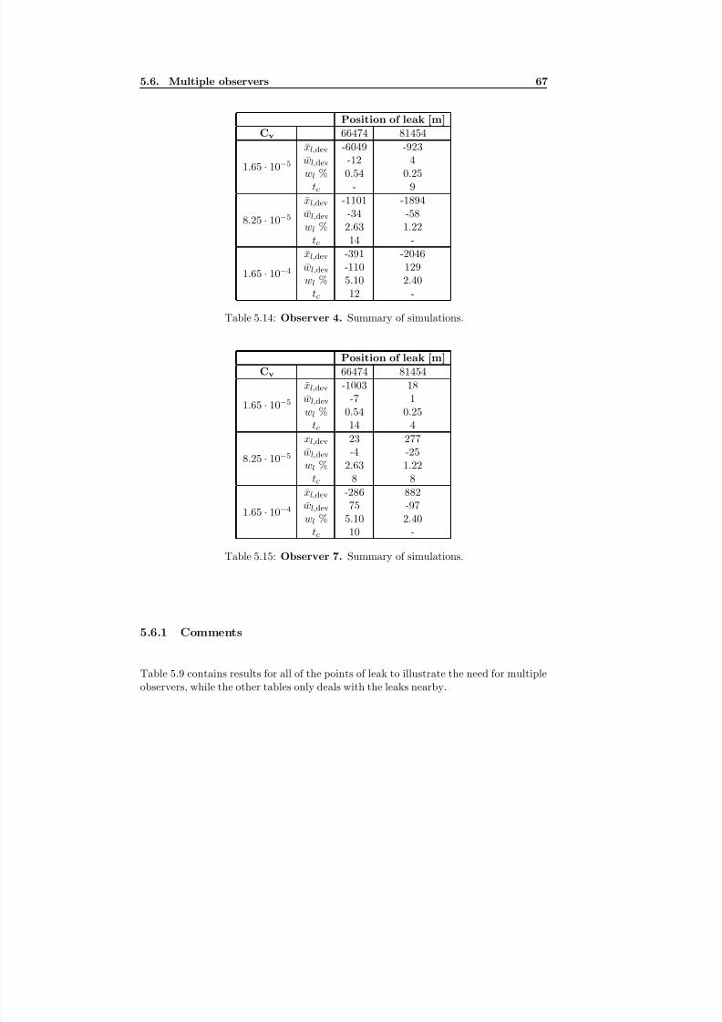
8/18/2019 Advanced Leak Detection using a Nonlinear Observer and OLGA
http://slidepdf.com/reader/full/advanced-leak-detection-using-a-nonlinear-observer-and-olga 75/131
5.6. Multiple observers 67
Position of leak [m]
Cv 66474 81454
1.65 · 10−5xl,dev -6049 -923wl,dev -12 4wl % 0.54 0.25
tc - 9
8.25 · 10−5
xl,dev -1101 -1894wl,dev -34 -58wl % 2.63 1.22
tc 14 -
1.65 · 10−4
xl,dev -391 -2046wl,dev -110 129wl % 5.10 2.40
tc 12 -
Table 5.14: Observer 4. Summary of simulations.
Position of leak [m]
Cv 66474 81454
1.65 · 10−5
xl,dev -1003 18wl,dev -7 1wl % 0.54 0.25
tc 14 4
8.25 · 10−5xl,dev 23 277wl,dev -4 -25wl % 2.63 1.22
tc 8 8
1.65 · 10−4
xl,dev -286 882wl,dev 75 -97wl % 5.10 2.40
tc 10 -
Table 5.15: Observer 7. Summary of simulations.
5.6.1 Comments
Table 5.9 contains results for all of the points of leak to illustrate the need for multipleobservers, while the other tables only deals with the leaks nearby.
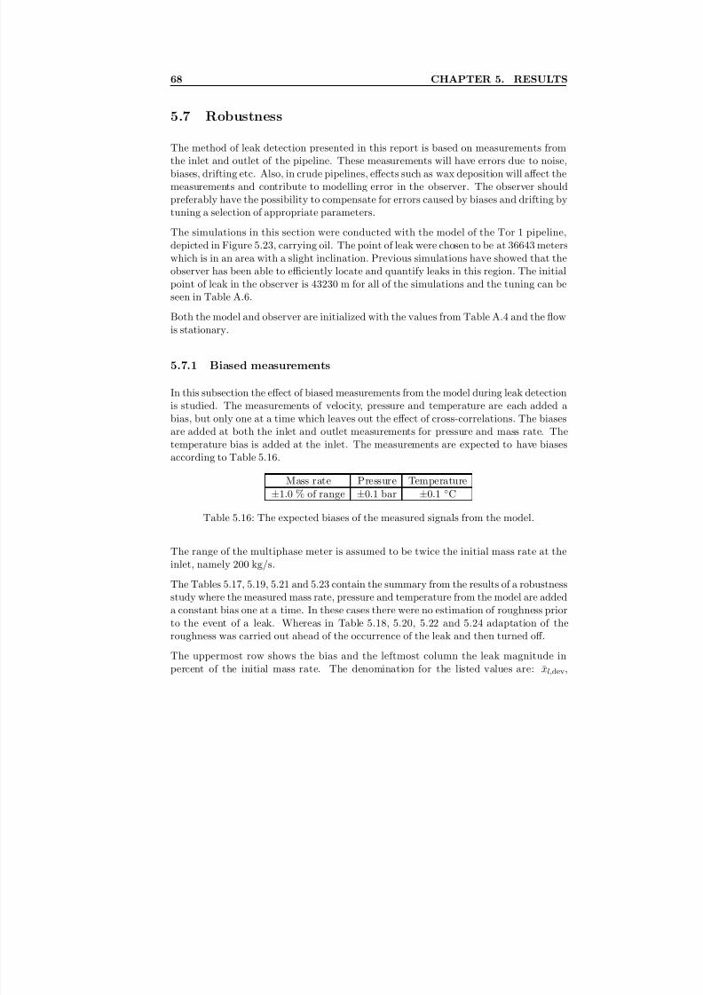
8/18/2019 Advanced Leak Detection using a Nonlinear Observer and OLGA
http://slidepdf.com/reader/full/advanced-leak-detection-using-a-nonlinear-observer-and-olga 76/131
68 CHAPTER 5. RESULTS
5.7 Robustness
The method of leak detection presented in this report is based on measurements fromthe inlet and outlet of the pipeline. These measurements will have errors due to noise,biases, drifting etc. Also, in crude pipelines, effects such as wax deposition will affect themeasurements and contribute to modelling error in the observer. The observer shouldpreferably have the possibility to compensate for errors caused by biases and drifting bytuning a selection of appropriate parameters.
The simulations in this section were conducted with the model of the Tor 1 pipeline,depicted in Figure 5.23, carrying oil. The point of leak were chosen to be at 36643 meterswhich is in an area with a slight inclination. Previous simulations have showed that theobserver has been able to efficiently locate and quantify leaks in this region. The initial
point of leak in the observer is 43230 m for all of the simulations and the tuning can beseen in Table A.6.
Both the model and observer are initialized with the values from Table A.4 and the flowis stationary.
5.7.1 Biased measurements
In this subsection the effect of biased measurements from the model during leak detectionis studied. The measurements of velocity, pressure and temperature are each added abias, but only one at a time which leaves out the effect of cross-correlations. The biasesare added at both the inlet and outlet measurements for pressure and mass rate. Thetemperature bias is added at the inlet. The measurements are expected to have biasesaccording to Table 5.16.
Mass rate Pressure Temperature
±1.0 % of range ±0.1 bar ±0.1 ◦C
Table 5.16: The expected biases of the measured signals from the model.
The range of the multiphase meter is assumed to be twice the initial mass rate at the
inlet, namely 200 kg/s.The Tables 5.17, 5.19, 5.21 and 5.23 contain the summary from the results of a robustnessstudy where the measured mass rate, pressure and temperature from the model are addeda constant bias one at a time. In these cases there were no estimation of roughness priorto the event of a leak. Whereas in Table 5.18, 5.20, 5.22 and 5.24 adaptation of theroughness was carried out ahead of the occurrence of the leak and then turned off.
The uppermost row shows the bias and the leftmost column the leak magnitude inpercent of the initial mass rate. The denomination for the listed values are: xl,dev,
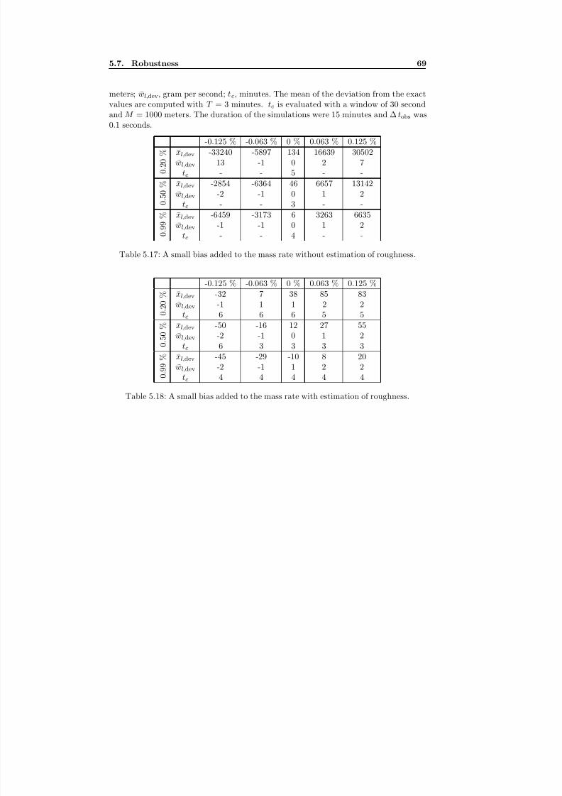
8/18/2019 Advanced Leak Detection using a Nonlinear Observer and OLGA
http://slidepdf.com/reader/full/advanced-leak-detection-using-a-nonlinear-observer-and-olga 77/131
5.7. Robustness 69
meters; wl,dev, gram per second; tc, minutes. The mean of the deviation from the exactvalues are computed with T = 3 minutes. tc is evaluated with a window of 30 second
and M = 1000 meters. The duration of the simulations were 15 minutes and ∆ tobs was0.1 seconds.
-0.125 % -0.063 % 0 % 0.063 % 0.125 %
0 . 2
0 % xl,dev -33240 -5897 134 16639 30502
wl,dev 13 -1 0 2 7tc - - 5 - -
0 . 5
0 % xl,dev -2854 -6364 46 6657 13142
wl,dev -2 -1 0 1 2tc - - 3 - -
0 . 9 9 % xl,dev -6459 -3173 6 3263 6635
wl,dev -1 -1 0 1 2tc - - 4 - -
Table 5.17: A small bias added to the mass rate without estimation of roughness.
-0.125 % -0.063 % 0 % 0.063 % 0.125 %
0 . 2
0 % xl,dev -32 7 38 85 83
wl,dev -1 1 1 2 2tc 6 6 6 5 5
0 . 5 0 % xl,dev -50 -16 12 27 55
wl,dev
-2 -1 0 1 2tc 6 3 3 3 3
0 . 9
9 % xl,dev -45 -29 -10 8 20
wl,dev -2 -1 1 2 2tc 4 4 4 4 4
Table 5.18: A small bias added to the mass rate with estimation of roughness.
8/18/2019 Advanced Leak Detection using a Nonlinear Observer and OLGA
http://slidepdf.com/reader/full/advanced-leak-detection-using-a-nonlinear-observer-and-olga 78/131
70 CHAPTER 5. RESULTS
-1.0 % -0.5 % 0 % 0.5 % 1.0 %
0 . 2
0 % xl,dev -47747 -47747 38 36555 36555
wl,dev 34 46 1 4 6tc - - 6 - -
0 . 5
0 % xl,dev -47747 -47747 12 36555 36555
wl,dev 93 133 0 9 11tc - - 3 - -
0 . 9
9 % xl,dev -47747 -47747 -10 27024 36555
wl,dev 204 -5 1 8 19tc - - 4 - -
Table 5.19: A relatively large bias added to the mass rate without estimation of rough-
ness.
-1.0 % -0.5 % 0 % 0.5 % 1.0 %
0 . 2
0 % xl,dev -943 -502 134 346 987
wl,dev -13 -7 0 6 12tc 14 6 5 5 14
0 . 5
0 % xl,dev -675 -264 46 192 650
wl,dev -15 -7 0 7 12tc 7 6 3 3 3
0 . 9 9
% xl,dev -512 -222 6 163 469wl,dev -14 -7 0 7 12
tc 7 6 4 4 4
Table 5.20: A relatively large bias added to the mass rate with estimation of roughness.
-0.10 bar -0.05 bar 0 bar 0.05 bar 0.10 bar
0 . 2
0 % xl,dev -3136 -493 134 1983 3564
wl,dev 1 1 0 -1 -1tc - - 5 - -
0 . 5
0 % xl,dev -201 -648 46 808 1381wl,dev 1 1 0 -1 -1
tc - 6 3 3 -
0 . 9
9 % xl,dev -686 -259 6 326 752
wl,dev 1 1 0 0 -1tc 7 6 4 4 10
Table 5.21: Perturbing pressure without estimation of the roughness.
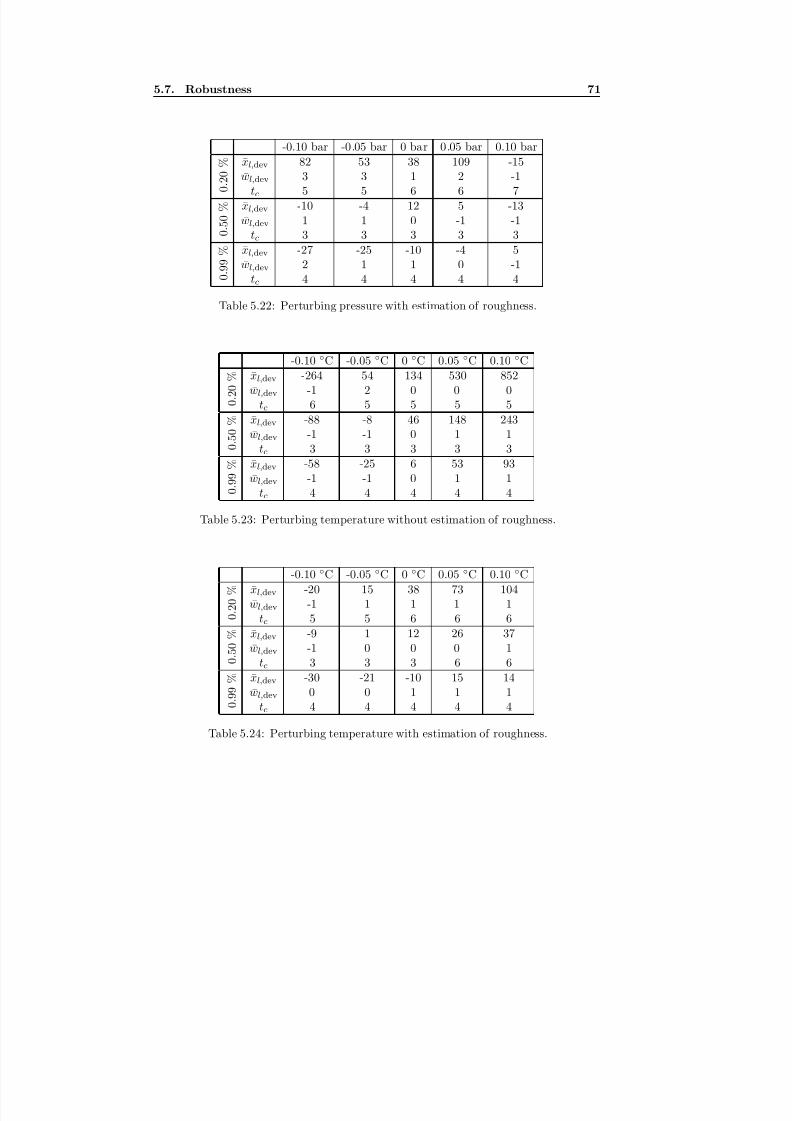
8/18/2019 Advanced Leak Detection using a Nonlinear Observer and OLGA
http://slidepdf.com/reader/full/advanced-leak-detection-using-a-nonlinear-observer-and-olga 79/131
5.7. Robustness 71
-0.10 bar -0.05 bar 0 bar 0.05 bar 0.10 bar
0 . 2
0 % xl,dev 82 53 38 109 -15
wl,dev 3 3 1 2 -1tc 5 5 6 6 7
0 . 5
0 % xl,dev -10 -4 12 5 -13
wl,dev 1 1 0 -1 -1tc 3 3 3 3 3
0 . 9
9 % xl,dev -27 -25 -10 -4 5
wl,dev 2 1 1 0 -1tc 4 4 4 4 4
Table 5.22: Perturbing pressure with estimation of roughness.
-0.10 ◦C -0.05 ◦C 0 ◦C 0.05 ◦C 0.10 ◦C
0 . 2
0 % xl,dev -264 54 134 530 852
wl,dev -1 2 0 0 0tc 6 5 5 5 5
0 . 5
0 % xl,dev -88 -8 46 148 243
wl,dev -1 -1 0 1 1tc 3 3 3 3 3
0 . 9
9 % xl,dev -58 -25 6 53 93
wl,dev -1 -1 0 1 1tc 4 4 4 4 4
Table 5.23: Perturbing temperature without estimation of roughness.
-0.10 ◦C -0.05 ◦C 0 ◦C 0.05 ◦C 0.10 ◦C
0 . 2
0 % xl,dev -20 15 38 73 104
wl,dev -1 1 1 1 1tc 5 5 6 6 6
0 . 5
0 %
xl,dev -9 1 12 26 37wl,dev -1 0 0 0 1tc 3 3 3 6 6
0 . 9
9 % xl,dev -30 -21 -10 15 14
wl,dev 0 0 1 1 1tc 4 4 4 4 4
Table 5.24: Perturbing temperature with estimation of roughness.
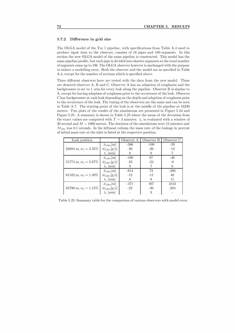
8/18/2019 Advanced Leak Detection using a Nonlinear Observer and OLGA
http://slidepdf.com/reader/full/advanced-leak-detection-using-a-nonlinear-observer-and-olga 80/131
72 CHAPTER 5. RESULTS
5.7.2 Difference in grid size
The OLGA model of the Tor 1 pipeline, with specifications from Table A.4 used toproduce input data to the observer, consists of 16 pipes and 100 segments. In thissection the new OLGA model of the same pipeline is constructed. This model has thesame pipeline profile, but each pipe is divided into shorter segments so the total numberof segments sums up to 198. The OLGA observer however is unchanged with the purposeto induce a modelling error. Both the observer and the model are as specified in TableA.4, except for the number of sections which is specified above.
Three different observers have are tested with the data from the new model. Theseare denoted observer A, B and C. Observer A has no adaption of roughness and thebackpressure is set to 1 atm for every leak along the pipeline. Observer B is similar to
A, except for having adaption of roughness prior to the occurrence of the leak. ObserverC has backpressure at each leak depending on the depth and adaption of roughness priorto the occurrence of the leak. The tuning of the observers are the same and can be seenin Table A.7. The starting point of the leak is at the middle of the pipeline at 43230meters. Two plots of the results of the simulations are presented in Figure 5.24 andFigure 5.25. A summary is shown in Table 5.25 where the mean of the deviation fromthe exact values are computed with T = 3 minutes. tc is evaluated with a window of 30 second and M = 1000 meters. The duration of the simulations were 15 minutes and∆tobs was 0.1 seconds. In the leftmost column the mass rate of the leakage in percentof initial mass rate at the inlet is listed at the respective position.
Leak position Observer A Observer B Observer C
23884 m, wl = 3.35%xl,dev[m] -566 -100 -29
wl,dev[g/s] -26 -26 -12tc [min] 8 8 7
51774 m, wl = 5.67%xl,dev[m] -160 67 -46
wl,dev[g/s] -23 -24 -8tc [min] 9 7 6
61102 m, wl = 1.49%xl,dev[m] -614 73 -386
wl,dev[g/s] -12 -11 40tc [min] 8 9 11
65790 m, wl = 1.15%
xl,dev[m] -471 467 3443
wl,dev[g/s] -22 -20 -284tc [min] - 9 -
Table 5.25: Summary table for the comparison of various observers with model error.
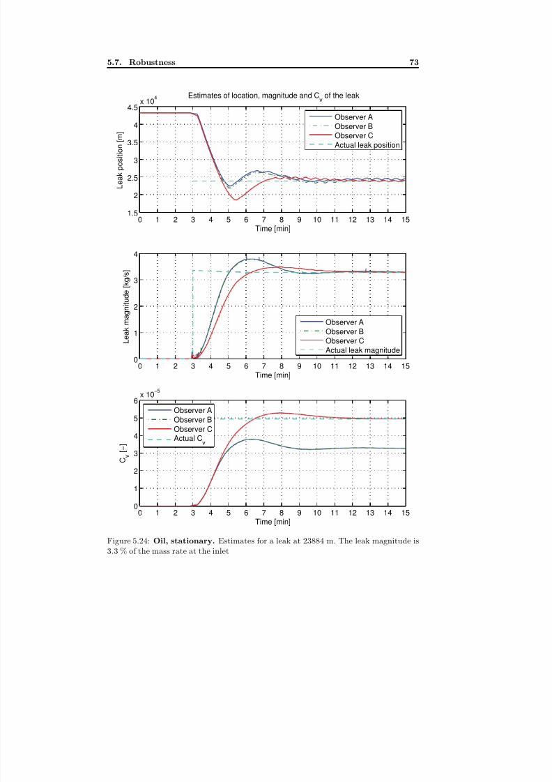
8/18/2019 Advanced Leak Detection using a Nonlinear Observer and OLGA
http://slidepdf.com/reader/full/advanced-leak-detection-using-a-nonlinear-observer-and-olga 81/131
5.7. Robustness 73
0 1 2 3 4 5 6 7 8 9 10 11 12 13 14 15
1.5
2
2.5
3
3.5
4
4.5
x 104 Estimates of location, magnitude and C
v of the leak
Time [min]
L e a k p o s i t i o n [ m ]
Observer A
Observer B
Observer C
Actual leak position
0 1 2 3 4 5 6 7 8 9 10 11 12 13 14 150
1
2
3
4
Time [min]
L e a
k m a g n i t u d e [ k g / s ]
Observer A
Observer BObserver C
Actual leak magnitude
0 1 2 3 4 5 6 7 8 9 10 11 12 13 14 150
1
2
3
4
5
6x 10
−5
Time [min]
C v
[ − ]
Observer A
Observer B
Observer CActual C
v
Figure 5.24: Oil, stationary. Estimates for a leak at 23884 m. The leak magnitude is3.3 % of the mass rate at the inlet
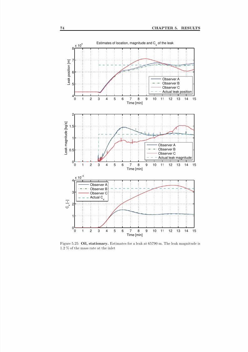
8/18/2019 Advanced Leak Detection using a Nonlinear Observer and OLGA
http://slidepdf.com/reader/full/advanced-leak-detection-using-a-nonlinear-observer-and-olga 82/131
74 CHAPTER 5. RESULTS
0 1 2 3 4 5 6 7 8 9 10 11 12 13 14 15
4
5
6
7
8
x 104 Estimates of location, magnitude and C
v of the leak
Time [min]
L e a k p o s i t i o n [ m ]
Observer A
Observer B
Observer C
Actual leak position
0 1 2 3 4 5 6 7 8 9 10 11 12 13 14 150
0.5
1
1.5
2
Time [min]
L e a
k m a g n i t u d e [ k g / s ]
Observer A
Observer BObserver C
Actual leak magnitude
0 1 2 3 4 5 6 7 8 9 10 11 12 13 14 150
1
2
3
4x 10
−5
Time [min]
C v
[ − ]
Observer A
Observer B
Observer CActual C
v
Figure 5.25: Oil, stationary. Estimates for a leak at 65790 m. The leak magnitude is1.2 % of the mass rate at the inlet
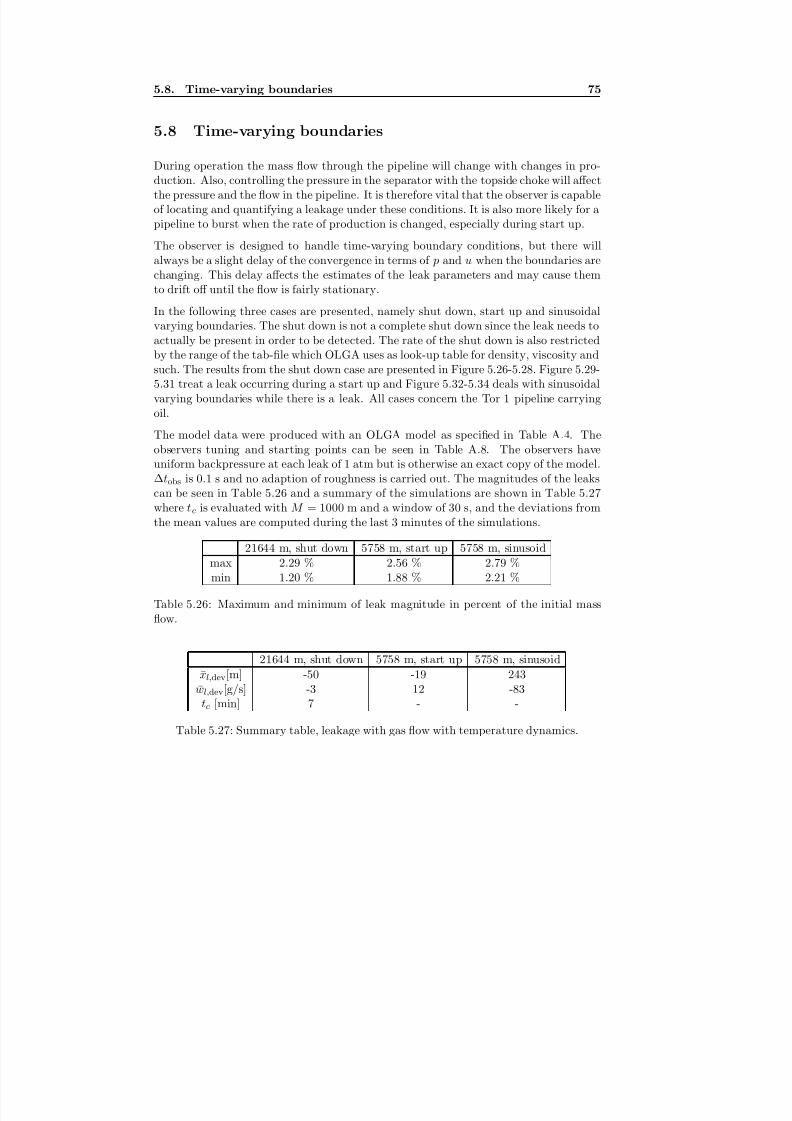
8/18/2019 Advanced Leak Detection using a Nonlinear Observer and OLGA
http://slidepdf.com/reader/full/advanced-leak-detection-using-a-nonlinear-observer-and-olga 83/131
5.8. Time-varying boundaries 75
5.8 Time-varying boundaries
During operation the mass flow through the pipeline will change with changes in pro-duction. Also, controlling the pressure in the separator with the topside choke will affectthe pressure and the flow in the pipeline. It is therefore vital that the observer is capableof locating and quantifying a leakage under these conditions. It is also more likely for apipeline to burst when the rate of production is changed, especially during start up.
The observer is designed to handle time-varying boundary conditions, but there willalways be a slight delay of the convergence in terms of p and u when the boundaries arechanging. This delay affects the estimates of the leak parameters and may cause themto drift off until the flow is fairly stationary.
In the following three cases are presented, namely shut down, start up and sinusoidalvarying boundaries. The shut down is not a complete shut down since the leak needs toactually be present in order to be detected. The rate of the shut down is also restrictedby the range of the tab-file which OLGA uses as look-up table for density, viscosity andsuch. The results from the shut down case are presented in Figure 5.26-5.28. Figure 5.29-5.31 treat a leak occurring during a start up and Figure 5.32-5.34 deals with sinusoidalvarying boundaries while there is a leak. All cases concern the Tor 1 pipeline carryingoil.
The model data were produced with an OLGA model as specified in Table A.4. Theobservers tuning and starting points can be seen in Table A.8. The observers haveuniform backpressure at each leak of 1 atm but is otherwise an exact copy of the model.
∆tobs is 0.1 s and no adaption of roughness is carried out. The magnitudes of the leakscan be seen in Table 5.26 and a summary of the simulations are shown in Table 5.27where tc is evaluated with M = 1000 m and a window of 30 s, and the deviations fromthe mean values are computed during the last 3 minutes of the simulations.
21644 m, shut down 5758 m, start up 5758 m, sinusoid
max 2.29 % 2.56 % 2.79 %min 1.20 % 1.88 % 2.21 %
Table 5.26: Maximum and minimum of leak magnitude in percent of the initial massflow.
21644 m, shut down 5758 m, start up 5758 m, sinusoid
xl,dev[m] -50 -19 243wl,dev[g/s] -3 12 -83
tc [min] 7 - -
Table 5.27: Summary table, leakage with gas flow with temperature dynamics.
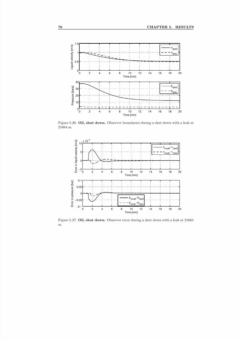
8/18/2019 Advanced Leak Detection using a Nonlinear Observer and OLGA
http://slidepdf.com/reader/full/advanced-leak-detection-using-a-nonlinear-observer-and-olga 84/131
76 CHAPTER 5. RESULTS
0 2 4 6 8 10 12 14 16 18 200
0.5
1
1.5
Time [min]
L i q u i d v e l o c i t y [ m
/ s ]
uobs0
uobsL
0 2 4 6 8 10 12 14 16 18 200
10
20
30
40
Time [min]
P r e s s u r e [ b a r a ] p
obs0
pobsL
Figure 5.26: Oil, shut down. Observer boundaries during a shut down with a leak at21664 m.
0 2 4 6 8 10 12 14 16 18 20−5
0
5
10x 10
−3
Time [min] E r r o r i n l i q u i d v e l o c i t y [ m / s ]
umod0
−uobs0
umodL
−uobsL
0 2 4 6 8 10 12 14 16 18 20−0.1
−0.05
0
0.05
0.1
Time [min]
E r r o r i n p r e
s s u r e [ b a r ]
pmod0
−pobs0
pmodL
−pobsL
Figure 5.27: Oil, shut down. Observer error during a shut down with a leak at 21664m.
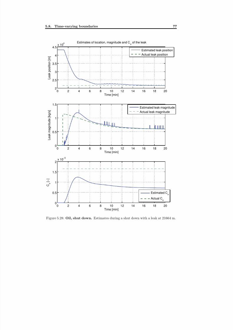
8/18/2019 Advanced Leak Detection using a Nonlinear Observer and OLGA
http://slidepdf.com/reader/full/advanced-leak-detection-using-a-nonlinear-observer-and-olga 85/131
5.8. Time-varying boundaries 77
0 2 4 6 8 10 12 14 16 18 202
2.5
3
3.5
4
4.5x 10
4 Estimates of location, magnitude and Cv of the leak
Time [min]
L e a k p o s i t i o n [ m ]
Estimated leak position
Actual leak position
0 2 4 6 8 10 12 14 16 18 200
0.5
1
1.5
Time [min]
L e a k m a g n i t u d e [ k g / s ]
Estimated leak magnitude
Actual leak magnitude
0 2 4 6 8 10 12 14 16 18 200
0.5
1
1.5
2x 10
−5
Time [min]
C v
[ − ]
Estimated Cv
Actual Cv
Figure 5.28: Oil, shut down. Estimates during a shut down with a leak at 21664 m.
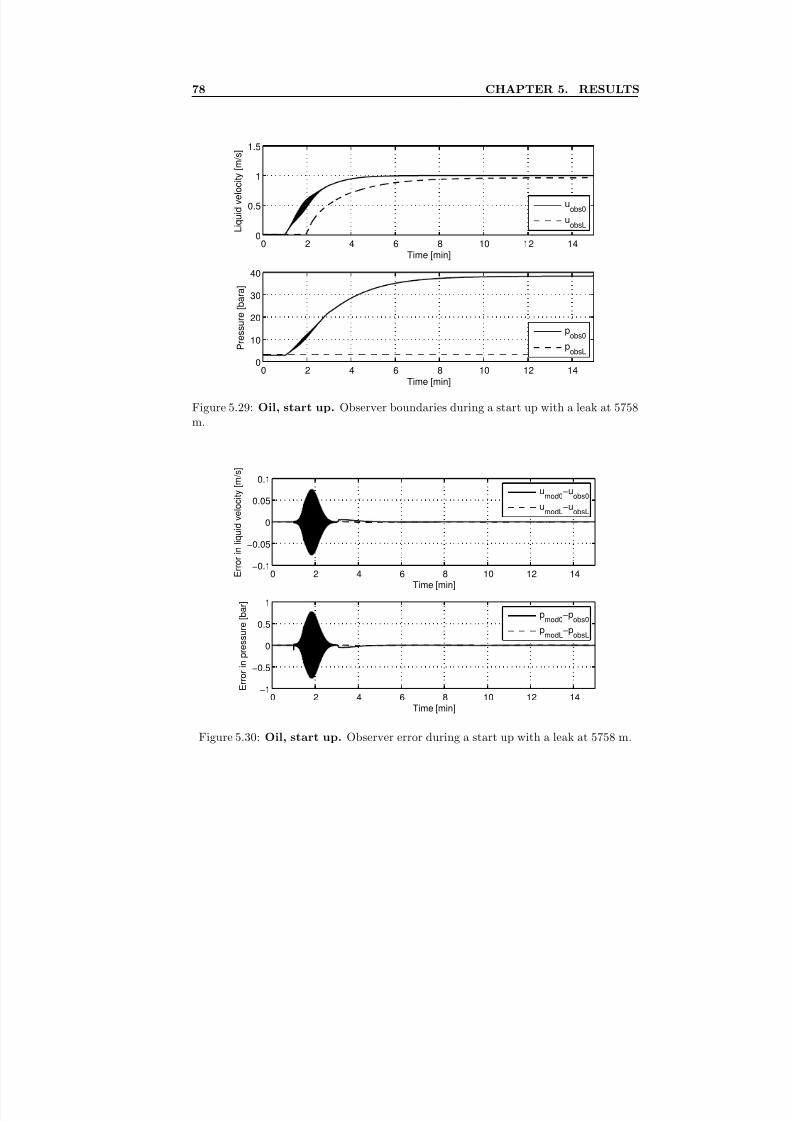
8/18/2019 Advanced Leak Detection using a Nonlinear Observer and OLGA
http://slidepdf.com/reader/full/advanced-leak-detection-using-a-nonlinear-observer-and-olga 86/131
78 CHAPTER 5. RESULTS
0 2 4 6 8 10 12 140
0.5
1
1.5
Time [min]
L i q u i d v e l o c i t y [ m /
s ]
uobs0
uobsL
0 2 4 6 8 10 12 140
10
20
30
40
Time [min]
P r e s s u r e [ b a r a ]
pobs0
pobsL
Figure 5.29: Oil, start up. Observer boundaries during a start up with a leak at 5758m.
0 2 4 6 8 10 12 14−0.1
−0.05
0
0.05
0.1
Time [min] E r r o r i n l i q u i d v e l o c i t y [ m
/ s ]
umod0
−uobs0
umodL
−uobsL
0 2 4 6 8 10 12 14−1
−0.5
0
0.5
1
Time [min]
E r r o r i n p r e s s
u r e [ b a r ]
pmod0
−pobs0
p
modL
−p
obsL
Figure 5.30: Oil, start up. Observer error during a start up with a leak at 5758 m.
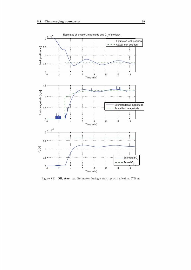
8/18/2019 Advanced Leak Detection using a Nonlinear Observer and OLGA
http://slidepdf.com/reader/full/advanced-leak-detection-using-a-nonlinear-observer-and-olga 87/131
5.8. Time-varying boundaries 79
0 2 4 6 8 10 12 140
0.5
1
1.5
2x 10
4 Estimates of location, magnitude and Cv of the leak
Time [min]
L e a k p o s i t i o n [ m ]
Estimated leak position
Actual leak position
0 2 4 6 8 10 12 140
0.5
1
1.5
Time [min]
L e a k m a g n i t u d e [ k g / s ]
Estimated leak magnitude
Actual leak magnitude
0 2 4 6 8 10 12 140
0.5
1
1.5
2x 10
−5
Time [min]
C v
[ − ]
Estimated Cv
Actual Cv
Figure 5.31: Oil, start up. Estimates during a start up with a leak at 5758 m.
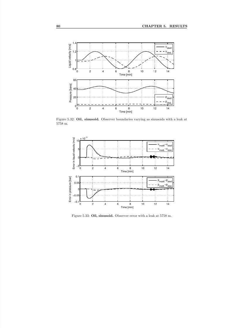
8/18/2019 Advanced Leak Detection using a Nonlinear Observer and OLGA
http://slidepdf.com/reader/full/advanced-leak-detection-using-a-nonlinear-observer-and-olga 88/131
80 CHAPTER 5. RESULTS
0 2 4 6 8 10 12 140.8
1
1.2
1.4
Time [min]
L i q u i d v e l o c i t y [ m /
s ]
uobs0
uobsL
0 2 4 6 8 10 12 140
20
40
60
Time [min]
P r e s s u r e [ b a r a ]
pobs0
pobsL
Figure 5.32: Oil, sinusoid. Observer boundaries varying as sinusoids with a leak at5758 m.
0 2 4 6 8 10 12 14−5
0
5
10x 10
−3
Time [min] E r r o r i n l i q u i d v e l o c i t y [ m / s ]
umod0
−uobs0
umodL
−uobsL
0 2 4 6 8 10 12 14−0.1
−0.05
0
0.05
0.1
Time [min]
E r r o r i n p r e s s
u r e [ b a r ]
pmod0
−pobs0
p
modL
−p
obsL
Figure 5.33: Oil, sinusoid. Observer error with a leak at 5758 m.
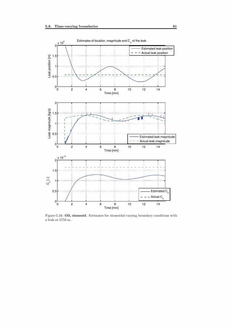
8/18/2019 Advanced Leak Detection using a Nonlinear Observer and OLGA
http://slidepdf.com/reader/full/advanced-leak-detection-using-a-nonlinear-observer-and-olga 89/131
5.8. Time-varying boundaries 81
0 2 4 6 8 10 12 140
0.5
1
1.5
2
x 104 Estimates of location, magnitude and C
v of the leak
Time [min]
L e a k p o s i t i o n [ m ]
Estimated leak position
Actual leak position
0 2 4 6 8 10 12 140
0.5
1
1.5
2
Time [min]
L e a k m a g n i t u d e [ k g / s ]
Estimated leak magnitude
Actual leak magnitude
0 2 4 6 8 10 12 140
0.5
1
1.5
2x 10
−5
Time [min]
C v
[ − ]
Estimated Cv
Actual Cv
Figure 5.34: Oil, sinusoid. Estimates for sinusoidal varying boundary conditions witha leak at 5758 m.
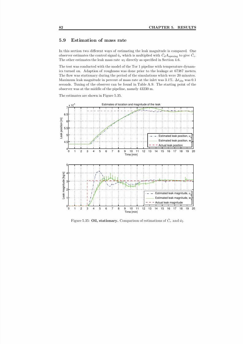
8/18/2019 Advanced Leak Detection using a Nonlinear Observer and OLGA
http://slidepdf.com/reader/full/advanced-leak-detection-using-a-nonlinear-observer-and-olga 90/131
82 CHAPTER 5. RESULTS
5.9 Estimation of mass rate
In this section two different ways of estimating the leak magnitude is compared. Oneobserver estimates the control signal us which is multiplied with C dAopening to give C v.The other estimates the leak mass rate wl directly as specified in Section 4.6.
The test was conducted with the model of the Tor 1 pipeline with temperature dynam-ics turned on. Adaption of roughness was done prior to the leakage at 67387 meters.The flow was stationary during the period of the simulations which were 20 minutes.Maximum leak magnitude in percent of mass rate at the inlet was 3.1%. ∆tobs was 0.1seconds. Tuning of the observer can be found in Table A.9. The starting point of theobserver was at the middle of the pipeline, namely 43230 m.
The estimates are shown in Figure 5.35.
0 1 2 3 4 5 6 7 8 9 10 11 12 13 14 15 16 17 18 19 204
4.5
5
5.5
6
6.5
7x 10
4 Estimates of location and magnitude of the leak
Time [min]
L e a k p o s i t i o n [ m ]
Estimated leak position, us
Estimated leak position, wl
Actual leak position
0 1 2 3 4 5 6 7 8 9 10 11 12 13 14 15 16 17 18 19 200
1
2
3
4
5
Time [min]
L e a k m a g n i t u d e [ k g / s ]
Estimated leak magnitude, us
Estimated leak magnitude, wl
Actual leak magnitude
Figure 5.35: Oil, stationary. Comparison of estimations of C v and wl.
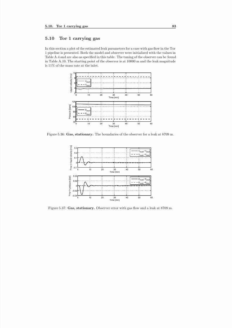
8/18/2019 Advanced Leak Detection using a Nonlinear Observer and OLGA
http://slidepdf.com/reader/full/advanced-leak-detection-using-a-nonlinear-observer-and-olga 91/131
5.10. Tor 1 carrying gas 83
5.10 Tor 1 carrying gas
In this section a plot of the estimated leak parameters for a case with gas flow in the Tor1 pipeline is presented. Both the model and observer were initialized with the values inTable A.4 and are also as specified in this table. The tuning of the observer can be foundin Table A.10. The starting point of the observer is at 10000 m and the leak magnitudeis 11% of the mass rate at the inlet.
0 10 20 30 40 50 602
4
6
8
10
Time [min]
L i q u i d v e l o c i t y [ m / s ]
uobs0
uobsL
0 10 20 30 40 50 6040
60
80
100
120
Time [min]
P r e s s u r e [ b a r a ]
pobs0
pobsL
Figure 5.36: Gas, stationary. The boundaries of the observer for a leak at 8709 m.
0 10 20 30 40 50 60−0.1
0
0.1
0.2
0.3
Time [min] E r r o r i n l i q u i d v e l o c i t y [ m / s ]
umod0
−uobs0
umodL
−uobsL
0 10 20 30 40 50 60−0.04
−0.02
0
0.02
0.04
Time [min]
E r r o r i n p r e s s u r e [ b a r ]
pmod0
−pobs0
pmodL
−pobsL
Figure 5.37: Gas, stationary. Observer error with gas flow and a leak at 8709 m.
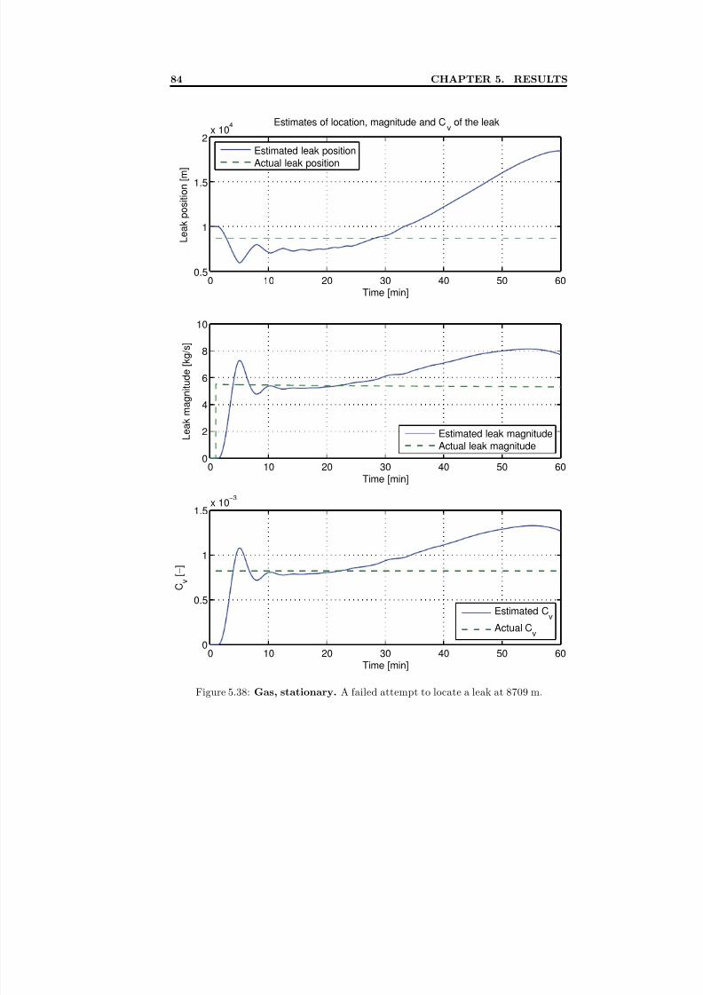
8/18/2019 Advanced Leak Detection using a Nonlinear Observer and OLGA
http://slidepdf.com/reader/full/advanced-leak-detection-using-a-nonlinear-observer-and-olga 92/131
84 CHAPTER 5. RESULTS
0 10 20 30 40 50 60
0.5
1
1.5
2
x 104 Estimates of location, magnitude and C
v of the leak
Time [min]
L e a k p o s i t i o n [ m ]
Estimated leak position
Actual leak position
0 10 20 30 40 50 600
2
4
6
8
10
Time [min]
L e a k m a g n i t u d e [ k g / s ]
Estimated leak magnitude
Actual leak magnitude
0 10 20 30 40 50 600
0.5
1
1.5x 10
−3
Time [min]
C v
[ − ]
Estimated Cv
Actual Cv
Figure 5.38: Gas, stationary. A failed attempt to locate a leak at 8709 m.
8/18/2019 Advanced Leak Detection using a Nonlinear Observer and OLGA
http://slidepdf.com/reader/full/advanced-leak-detection-using-a-nonlinear-observer-and-olga 93/131
8/18/2019 Advanced Leak Detection using a Nonlinear Observer and OLGA
http://slidepdf.com/reader/full/advanced-leak-detection-using-a-nonlinear-observer-and-olga 94/131
86 CHAPTER 5. RESULTS
valve equation from the one used in this work. For the case with time-varying boundariesthere was a minor difference from the former case mentioned due to ripples in the plot
of the ratio. These ripples were small compared to the ratio and would most likely notaffect the adaption of C v noticeably. Simulations covering a wide range of cases haveshown that the modelling is sufficiently accurate, and can also be said to be robust dueto its simplicity. Comparing a simulation of the estimation of mass rate to another withestimation of C v, demonstrated the benefits of the latter scheme. With only one casesupporting this claim, more effort could have been spent on tuning and testing withadaption of wl to get a broader set of results, but this type of research was not the scopeof this thesis and was therefore neglected.
The method of distributing the leakage over two nodes showed not to be as well suitedas expected since it was in need of a uniform grid to keep f l,1 and f l,2 positive or zero
for all possible leak positions. This problem was dealt with by using logic which keptthe two leakages positive under all circumstances. There is a possible problem with thissolution which could occur when the leakage in the observer is supposed to be sharedover two nodes but is only present in one node. This could restrain the adaption of the position since the seemingly continuous movement of the leakage stops. But thisissue has never emerged during simulations, most likely because the observer is excitedthrough the nonlinearity in the update law for the position adaption.
The work done in (Hauge, 2006) involved an observer written in Matlab which was testedwith a model also written in Matlab. It was therefore desirable to test this observer withdata produced with a state of the art computational fluid dynamics simulator, namelyOLGA. Comparing the estimates for the Matlab observer with the ones from the OLGAobserver indicated that the OLGA observer was superior in all cases, but the Matlabobserver performed decently for the cases with stationary flow in pipelines carrying oil.This justifies the simplifications made during the mathematical modelling, but the lackof an energy equation makes the Matlab model to simple for practical use.
Since OLGA supports simulations with temperature dynamics, new tests with gas flowin a straight pipeline was conducted. Incorporating temperature as a factor duringsimulations with gas flow, adds a realistic flavor that earlier has been missing. Thesetests showed that for a straight pipe, employing output injection worked and a small leakof gas could be detected during stationary flow with great accuracy. For the cases withsinusoidal varying boundary conditions the position estimate was not very accurate, but
at least the location was narrowed down to the first half of the pipeline. As for the casewith shut down, it takes about two minutes for the observer to respond to the leak. Thisis most likely due to the reduction in pressure at the outlet causing a drastic increasein velocity, which again causes the estimated magnitude to be negative during this timespan. When the flow has settled, both magnitude and position are correctly estimatedwithin 6 minutes.
Unfortunately, applying output injection to an observer, not initialized with the exactsame values as the model, monitoring the Tor 1 pipeline carrying gas, resulted in the
8/18/2019 Advanced Leak Detection using a Nonlinear Observer and OLGA
http://slidepdf.com/reader/full/advanced-leak-detection-using-a-nonlinear-observer-and-olga 95/131
5.11. Discussion 87
pressure exceeding the values bounded by the tab-file which is used as look-up tablefor fluid properties. For this case the mass rate at the inlet in the observer deviated
with -1 kg/s from the model during initialization. The reason for the sudden increasein pressure is not certain, but could have been caused by wrong modelling of the gasflow in the mathematical model since it neither does incorporate the effect of gravityor temperature. This could result in the wrong boundary conditions for the observeremploying output injection. The results mentioned above have been omitted due tonot being very descriptive. Another case with the Tor 1 pipeline carrying gas was alsotested, but in this case the observer was initialized with the exact same boundaries asthe model. This worked out fine even with k0 = kL = 0, which is maximum observergain, but the observer was not capable of locating any leaks. It seems as if the signatureleft in the measurements of velocity and pressure by the leak is too weak for it to belocated, even though the magnitude of the leakage is rather large. There might also be a
chance that the leakage affects the boundaries of the model with such impact that theyno longer can be called stationary.
As seen in the section dealing with time-varying boundary conditions, some problemsemerged when locating the leakage. First off, when applying sinusoidal boundary condi-tions, the position estimate fluctuated with approximately the same period as the liquidvelocity at the inlet. This is due to the observer not being able to track the boundariesof the observer without a slight delay. This delay results in an error which again affectsthe estimated leak parameters. By inspecting the plots of xl and the leak magnitude forthe start up and shut down cases, it is clear that the position estimate does not convergeuntil the boundaries reach a steady state. Another issue also arises with time-varying
boundary conditions, namely: for what leak magnitude should the observer signalize aleak? With the observer lagging behind the model there might be a chance that theerror is sufficiently large to affect the estimated magnitude of the leak and result in afalse alarm.
With the Tor 1 pipeline carrying oil, multiple observers were used to locate and quantifyleakages. It was shown that the multiple observers with different tuning and startingpoint would induce greater certainty for the estimates. Also, introducing observers wherethe backpressure was the same for each of the leaks along the pipeline, proved to be moreeffective than the intuitive setup with ambient pressure dependent on the sea depth. Thepositive effects with uniform backpressure trigger the thought of setting the backpressureat each leak to a constant value depending on the pressure inside the pipe. The result
would be that the differential pressure over all of the leaks along the pipeline would beapproximately the same, and this might cause the estimated leak parameters to convergemore rapidly in areas with steep inclinations of the pipeline.
The weak spot of the model-based observer presented in this thesis is its sensitivity tobiased and drifting measurements which causes vast errors in the position estimate. Theestimated magnitude of the leak, on the other hand, is relatively robust to these kindsof error, but this is of less importance than the position. Adaption of roughness priorto the leakage compensates for the differences between the observer and model causing
8/18/2019 Advanced Leak Detection using a Nonlinear Observer and OLGA
http://slidepdf.com/reader/full/advanced-leak-detection-using-a-nonlinear-observer-and-olga 96/131
88 CHAPTER 5. RESULTS
erroneous estimates, but this was only tested for cases with one biased measurementat a time. Even though the following problem was not encountered in this work, there
could be cases where the adaption of roughness is not sufficient to compensate for biasesand drifting. In such cases it might be possible to utilize the built-in support in theOLGAMatlabToolbox to adjust the pipeline diameter in the OLGA observer. Thiscould most likely be done in a similar manner as with the pipeline roughness by usingthe same update law with a slower tuning.
5.11.1 Future work
It would be interesting to conduct a rigorous study of robustness with measurementsfrom operational pipelines, but this is of course difficult since leaks seldom occurs and
not can be induced. Instead it would be desirable to carry out experiments with a scaledtest rig to see if the benefits of the model-based observer would still be applicable.
There has not been established any proofs of convergence for the update laws, butnumerous simulations indicate that the estimated values will converge to the correctvalue with stationary boundary conditions. These proofs are vital for the acceptanceof the adaptive, model-based observer in the engineering communities, and this is whyfuture work should focus on laying such a theoretical foundation. There are neither anyproofs showing that output injection will work with time-varying boundary conditionsor that output injection should work with the OLGA observer with a pipeline followingthe seabed and incorporating temperature dynamics.
Since the OLGA observer works with one-phase flow of both oil and gas in straight,horizontal pipelines, it is not unthinkable that it might work for two-phase flow. Itwould most likely require modification of the observer presented in this thesis. Thiscould be modifications such as a new valve equation and different boundary conditions.
Another interesting aspect of the observer which can be investigated, is whether runningmultiple simulations with the same set of data while resetting the starting point of xl
and us to best ones available between the simulations will improve precision. The bestones in this context would be the ones which are obtained last. If this procedure seemsto work, it might be possible to locate leaks during fast shut downs where the leakagedisappears after a short period of time.
8/18/2019 Advanced Leak Detection using a Nonlinear Observer and OLGA
http://slidepdf.com/reader/full/advanced-leak-detection-using-a-nonlinear-observer-and-olga 97/131
89
Chapter 6
Conclusions
The adaptive Luenberger-type observer presented in this thesis employs OLGA as itscomputational fluid dynamics simulator which is a state of the art simulator for one-,two- and three-phase flow. The OLGA observer is manipulated through Matlab whichmake it possible to make use of output injection in form of boundary conditions, controlthe magnitude and position of the estimated leakage and adapt roughness to compensatefor model errors and biased measurements. The OLGA observer has numerous advan-tages over its predecessor, i.e. the observer constructed with Matlab in (Hauge, 2006),among which the incorporation of temperature dynamics, the support for pipelines withdifference in altitude, no need for uniform grid and that it is widely used by oil companies
are the most important ones.Setting up an OLGA observer is time consuming, especially if there is no OLGA modelwhich can be used as a basis. The observer bases its estimates on measurements of pressure, velocity and temperature from the inlet and pressure and velocity from theoutlet. These measurements are usually available for newer pipelines and can easily belogged or low-pass filtered and fed directly to the observer. If data are logged, it ispossible to run simulations repeatedly after a leak has been detected, but not located.This makes it possible to use the observer after the pipeline has been shut down.
Simulations with a straight, horizontal pipeline showed that the OLGA observer wassuperior to the Matlab observer constructed in (Hauge, 2006) with both oil and gas
flow, and without any temperature dynamics. The OLGA observer was also testedwith small leakages in a straight, horizontal pipeline carrying gas, where temperaturedynamics was turned on. This yielded promising results.
An observer for an actual pipeline was also constructed in OLGA and tests were carriedout with data from an existing OLGA model provided by Statoil. These tests revealedthe need for multiple observers along long pipelines with difference in height. Beneficialeffects for observers with uniform backpressure at each leak were also shown.
Numerous simulations with biased inputs to the observer identified a need for some kind

8/18/2019 Advanced Leak Detection using a Nonlinear Observer and OLGA
http://slidepdf.com/reader/full/advanced-leak-detection-using-a-nonlinear-observer-and-olga 98/131
90 CHAPTER 6. CONCLUSIONS
of internal compensation to take care of the position estimate which was highly affectedby the incorrect measurements. This problem was fixed by adapting the roughness
ahead of the occurrence of the leak and keeping it constant during localization andquantification. The estimated magnitude did not suffer from the same sensitivity tobiased measurements as the position estimate.
Simulations conducted with time-varying boundary conditions showed that the observerwas capable of detecting leaks in cases such as start up, shut down and with sinusoidalvarying boundary conditions.
OLGA proved to be well suited for the task as fluid simulator for the model-basedobserver. It has the essential features such as controllable leaks, sources and pressurenodes, and an interface which makes it possible to manipulate them through Matlab.
8/18/2019 Advanced Leak Detection using a Nonlinear Observer and OLGA
http://slidepdf.com/reader/full/advanced-leak-detection-using-a-nonlinear-observer-and-olga 99/131
91
References
O. M. Aamo, J. Salvesen, and B. A. Foss. Observer design using boundary injectionsfor pipeline monitoring and leak detection. 2005. Accepted for the Adchem 2006
Conference held at Gramado, Brazil, April 2-5 2006.
L. Billmann and R. Isermann. Leak detection methods for pipelines. Automatica , 23:381–385, 1987.
H. E. Emara-Shabaik, A. E. Khulief, and I. Hussaini. A non-linear multiple-model stateestimation scheme for pipeline leak detection and isolation. Journal of Systems and
Control Engineering , 216:497–512, 2002.
J. Feng, H Zhang, and D. Liu. Applications of fuzzy decision-making in pipeline leaklocalization. In Proceedings of IEEE International Conference on Fuzzy Systems, 2004,volume 2, pages 599–603, 2004.
E. Hauge. Leak detection for oil and gas pipelines with time varying boundary conditions.Technical report, NTNU, 2006.
R. Hu, H. Ye, G. Wang, and C. Lu. Leak detection in pipelines based on PCA. In Pro-
ceedings of the 8th IEEE International Conference on Control, Automation, Robotics
and Vision, 2004, volume 3, pages 1985–1989, 2004.
W. Ming and W. Wei-qiang. Application of wavelet to detect pipeline leak point. InProceedings of the sixth International Conference on Intelligent Systems Design and
Applications , 2006.
C. R. Nilssen. Leak detection for oil and gas pipelines by parameter and state estimation.Master’s thesis, NTNU, 2006.
OLGA User Manual, version 5 . Scandpower Petroleum Technology, a.
Users’s Manual OLGA - Matlab toolbox, version 1.01. Scandpower Petroleum Technol-ogy, b.
J. A. Schetz and A. E. Fuhs. Fundamentals of Fluid Mechanics , volume 1 of Handbook
of fluid dynamics and fluid machinery . John Wiley and Sons, 1996.

8/18/2019 Advanced Leak Detection using a Nonlinear Observer and OLGA
http://slidepdf.com/reader/full/advanced-leak-detection-using-a-nonlinear-observer-and-olga 100/131
92 CHAPTER 6. CONCLUSIONS
C. Verde. Multi-leak detection and isolation in fluid pipelines. Control Engineering
Practice , 9:467–472, 2001.
F. M. White. Fluid Mechanics . McGraw-Hill, fifth edition, 2003.
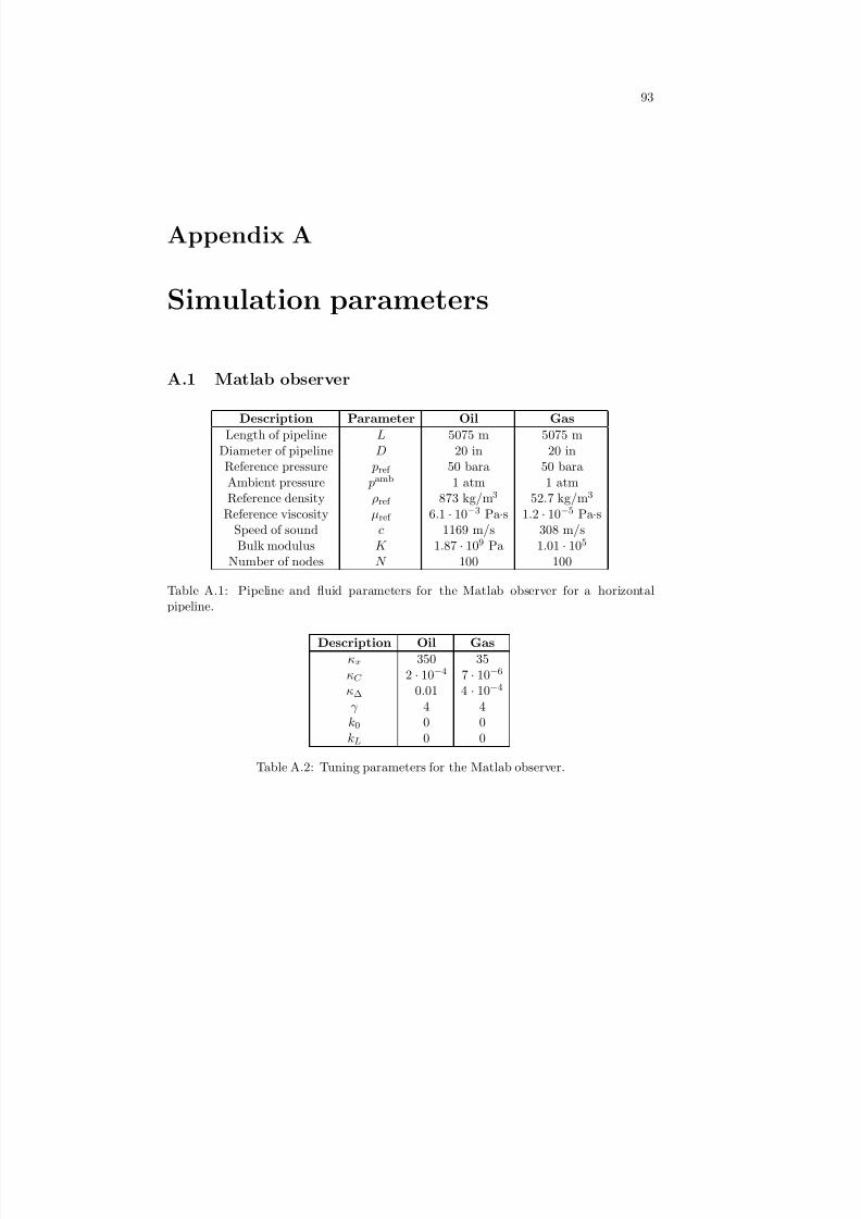
8/18/2019 Advanced Leak Detection using a Nonlinear Observer and OLGA
http://slidepdf.com/reader/full/advanced-leak-detection-using-a-nonlinear-observer-and-olga 101/131
93
Appendix A
Simulation parameters
A.1 Matlab observer
Description Parameter Oil Gas
Length of pipeline L 5075 m 5075 mDiameter of pipeline D 20 in 20 in
Reference pressure pref 50 bara 50 baraAmbient pressure pamb 1 atm 1 atmReference density ρref 873 kg/m3 52.7 kg/m3
Reference viscosity µref 6.1 · 10
−3
Pa·s 1.2 · 10
−5
Pa·sSpeed of sound c 1169 m/s 308 m/sBulk modulus K 1.87 · 109 Pa 1.01 · 105
Number of nodes N 100 100
Table A.1: Pipeline and fluid parameters for the Matlab observer for a horizontalpipeline.
Description Oil Gas
κx 350 35κC 2 · 10−4 7 · 10−6
κ∆ 0.01 4 · 10−4
γ 4 4k0 0 0kL 0 0
Table A.2: Tuning parameters for the Matlab observer.
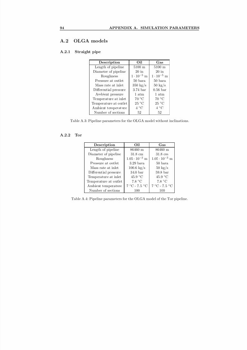
8/18/2019 Advanced Leak Detection using a Nonlinear Observer and OLGA
http://slidepdf.com/reader/full/advanced-leak-detection-using-a-nonlinear-observer-and-olga 102/131
94 APPENDIX A. SIMULATION PARAMETERS
A.2 OLGA models
A.2.1 Straight pipe
Description Oil Gas
Length of pipeline 5100 m 5100 mDiameter of pipeline 20 in 20 in
Roughness 1 · 10−5 m 1 · 10−5 mPressure at outlet 50 bara 50 baraMass rate at inlet 350 kg/s 50 kg/s
Differential pressure 3.74 bar 0.56 barAmbient pressure 1 atm 1 atm
Temperature at inlet 70 ◦
C 70 ◦
CTemperature at outlet 25 ◦C 25 ◦CAmbient temperature 4 ◦C 4 ◦C
Number of sections 52 52
Table A.3: Pipeline parameters for the OLGA model without inclinations.
A.2.2 Tor
Description Oil Gas
Length of pipeline 86460 m 86460 mDiameter of pipeline 31.8 cm 31.8 cm
Roughness 1.05 · 10−3 m 1.05 · 10−3 mPressure at outlet 3.29 bara 50 baraMass rate at inlet 100.6 kg/s 50 kg/s
Differential pressure 34.0 bar 59.8 barTemperature at inlet 45.9 ◦C 45.9 ◦C
Temperature at outlet 7.8 ◦C 7.8 ◦CAmbient temperature 7 ◦C - 7.5 ◦C 7 ◦C - 7.5 ◦C
Number of sections 100 100
Table A.4: Pipeline parameters for the OLGA model of the Tor pipeline.
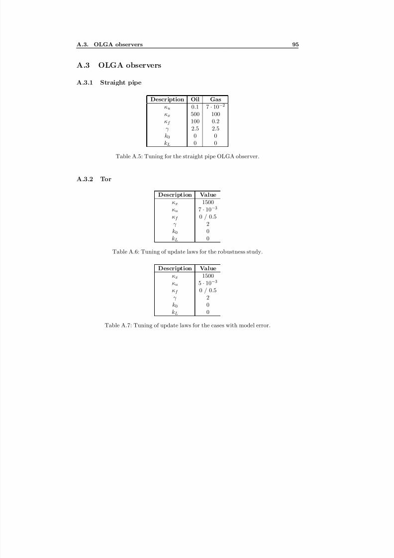
8/18/2019 Advanced Leak Detection using a Nonlinear Observer and OLGA
http://slidepdf.com/reader/full/advanced-leak-detection-using-a-nonlinear-observer-and-olga 103/131
A.3. OLGA observers 95
A.3 OLGA observers
A.3.1 Straight pipe
Description Oil Gas
κu 0.1 7 · 10−2
κx 500 100κf 100 0.2γ 2.5 2.5k0 0 0kL 0 0
Table A.5: Tuning for the straight pipe OLGA observer.
A.3.2 Tor
Description Value
κx 1500κu 7 · 10−3
κf 0 / 0.5γ 2k0 0
kL 0
Table A.6: Tuning of update laws for the robustness study.
Description Value
κx 1500κu 5 · 10−3
κf 0 / 0.5γ 2k0 0kL 0
Table A.7: Tuning of update laws for the cases with model error.
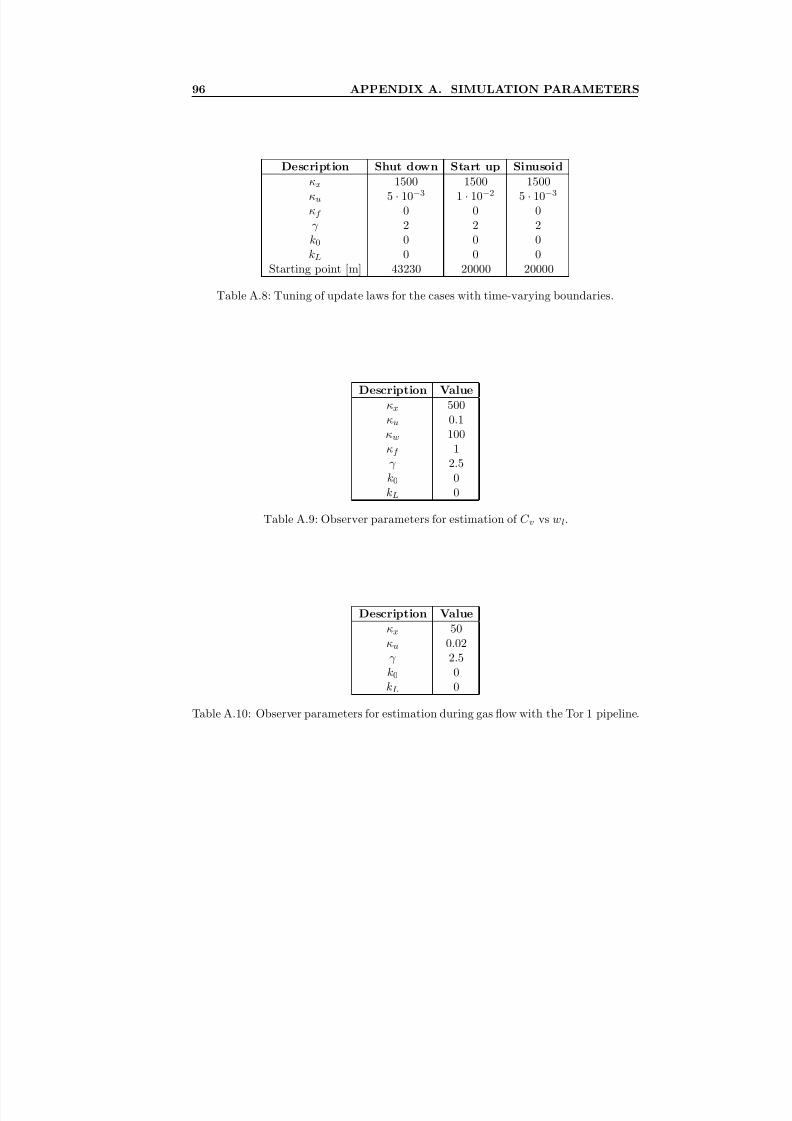
8/18/2019 Advanced Leak Detection using a Nonlinear Observer and OLGA
http://slidepdf.com/reader/full/advanced-leak-detection-using-a-nonlinear-observer-and-olga 104/131
96 APPENDIX A. SIMULATION PARAMETERS
Description Shut down Start up Sinusoid
κx 1500 1500 1500κu 5 · 10−3 1 · 10−2 5 · 10−3
κf 0 0 0γ 2 2 2k0 0 0 0kL 0 0 0
Starting point [m] 43230 20000 20000
Table A.8: Tuning of update laws for the cases with time-varying boundaries.
Description Value
κx 500κu 0.1κw 100κf 1γ 2.5
k0 0kL 0
Table A.9: Observer parameters for estimation of C v vs wl.
Description Value
κx 50
κu 0.02γ 2.5k0 0kL 0
Table A.10: Observer parameters for estimation during gas flow with the Tor 1 pipeline.
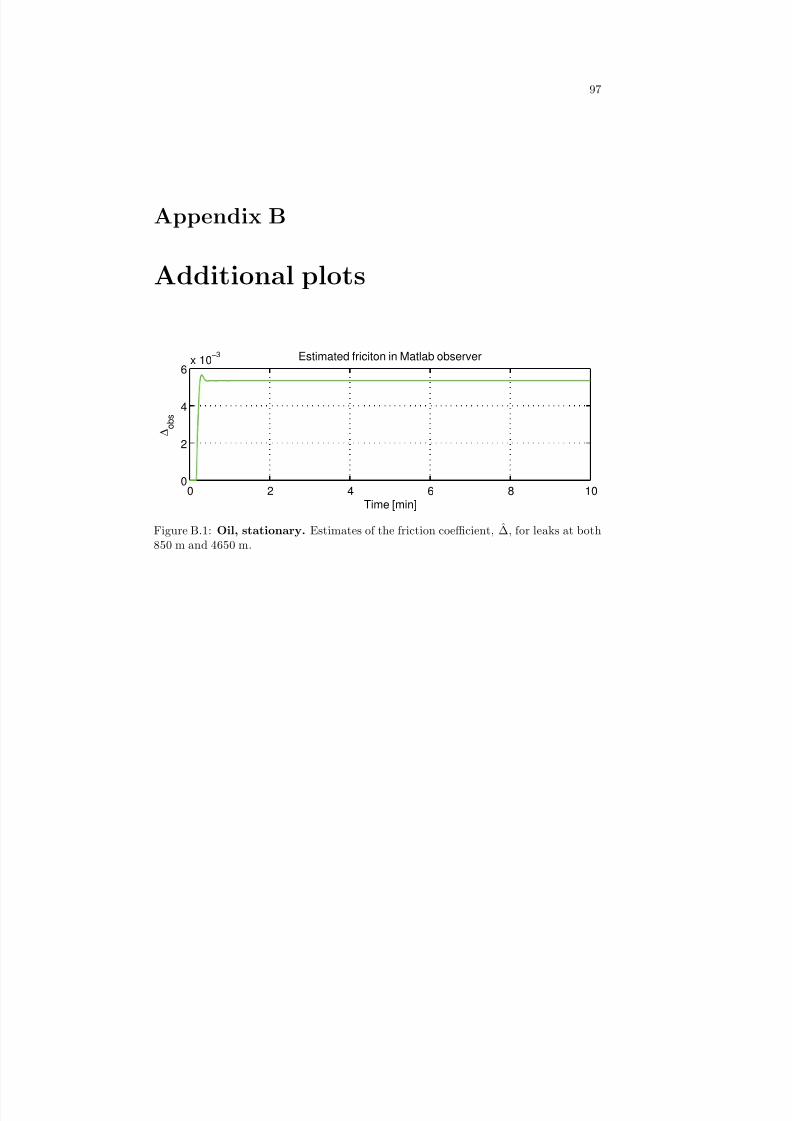
8/18/2019 Advanced Leak Detection using a Nonlinear Observer and OLGA
http://slidepdf.com/reader/full/advanced-leak-detection-using-a-nonlinear-observer-and-olga 105/131
97
Appendix B
Additional plots
0 2 4 6 8 100
2
4
6x 10
−3 Estimated friciton in Matlab observer
∆ o b s
Time [min]
Figure B.1: Oil, stationary. Estimates of the friction coefficient, ∆, for leaks at both850 m and 4650 m.
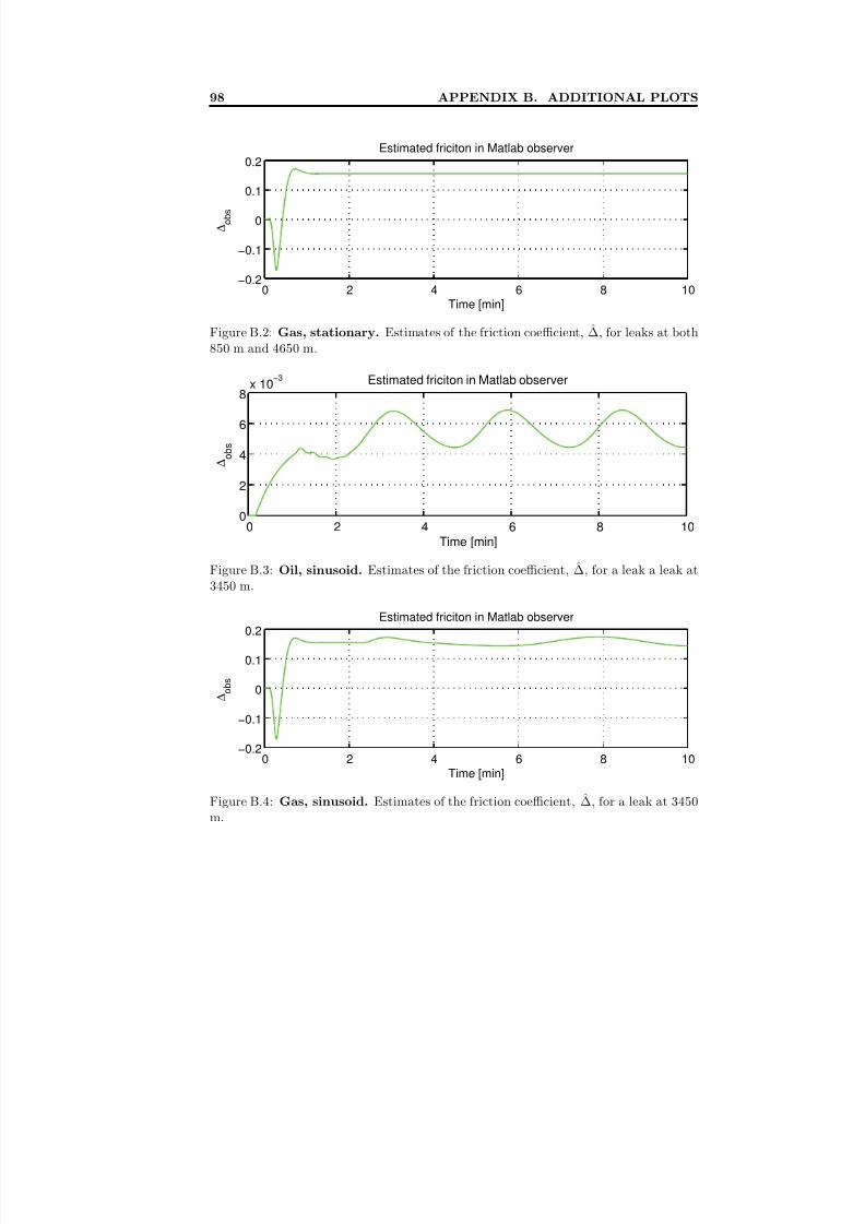
8/18/2019 Advanced Leak Detection using a Nonlinear Observer and OLGA
http://slidepdf.com/reader/full/advanced-leak-detection-using-a-nonlinear-observer-and-olga 106/131
98 APPENDIX B. ADDITIONAL PLOTS
0 2 4 6 8 10−0.2
−0.1
0
0.1
0.2Estimated friciton in Matlab observer
∆ o b s
Time [min]
Figure B.2: Gas, stationary. Estimates of the friction coefficient, ∆, for leaks at both
850 m and 4650 m.
0 2 4 6 8 100
2
4
6
8x 10
−3 Estimated friciton in Matlab observer
∆ o b s
Time [min]
Figure B.3: Oil, sinusoid. Estimates of the friction coefficient, ∆, for a leak a leak at3450 m.
0 2 4 6 8 10−0.2
−0.1
0
0.1
0.2Estimated friciton in Matlab observer
∆
o b s
Time [min]
Figure B.4: Gas, sinusoid. Estimates of the friction coefficient, ∆, for a leak at 3450m.
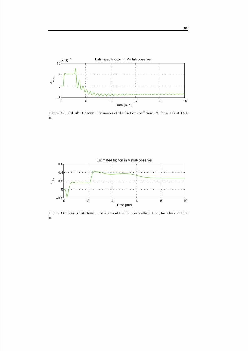
8/18/2019 Advanced Leak Detection using a Nonlinear Observer and OLGA
http://slidepdf.com/reader/full/advanced-leak-detection-using-a-nonlinear-observer-and-olga 107/131
99
0 2 4 6 8 10−5
0
5
10x 10
−3 Estimated friciton in Matlab observer
∆ o b s
Time [min]
Figure B.5: Oil, shut down. Estimates of the friction coefficient, ∆, for a leak at 1350m.
0 2 4 6 8 10−0.2
0
0.2
0.4
0.6Estimated friciton in Matlab observer
∆ o b s
Time [min]
Figure B.6: Gas, shut down. Estimates of the friction coefficient, ∆, for a leak at 1350m.
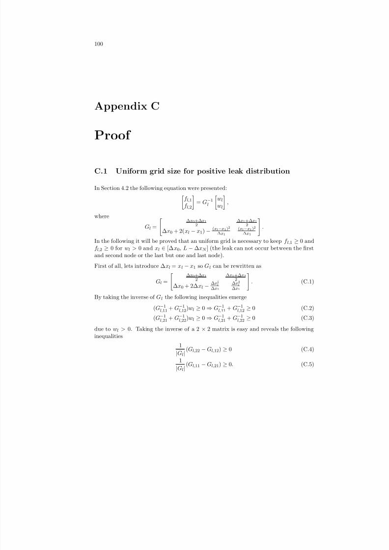
8/18/2019 Advanced Leak Detection using a Nonlinear Observer and OLGA
http://slidepdf.com/reader/full/advanced-leak-detection-using-a-nonlinear-observer-and-olga 108/131
100
Appendix C
Proof
C.1 Uniform grid size for positive leak distribution
In Section 4.2 the following equation were presented:f l,1f l,2
= G−1
l
wl
wl
,
where
Gl = ∆x0+∆x1
2∆x1+∆x2
2
∆x0 + 2(xl
−x1)
− (xl−x1)2
∆x1
(xl−x1)2
∆x1 .
In the following it will be proved that an uniform grid is necessary to keep f l,1 ≥ 0 andf l,2 ≥ 0 for wl > 0 and xl ∈ [∆x0, L − ∆xN ] (the leak can not occur between the firstand second node or the last but one and last node).
First of all, lets introduce ∆xl = xl − x1 so Gl can be rewritten as
Gl =
∆x0+∆x1
2∆x1+∆x2
2
∆x0 + 2∆xl − ∆x2l∆x1
∆x2l∆x1
. (C.1)
By taking the inverse of Gl the following inequalities emerge
(G−1l,11 + G−1
l,12)wl
≥0
⇒G−1
l,11 + G−1l,12
≥0 (C.2)
(G−1l,21 + G−1
l,22)wl ≥ 0 ⇒ G−1l,21 + G−1
l,22 ≥ 0 (C.3)
due to wl > 0. Taking the inverse of a 2 × 2 matrix is easy and reveals the followinginequalities
1
|Gl|(Gl,22 −Gl,12) ≥ 0 (C.4)
1
|Gl|(Gl,11 −Gl,21) ≥ 0. (C.5)
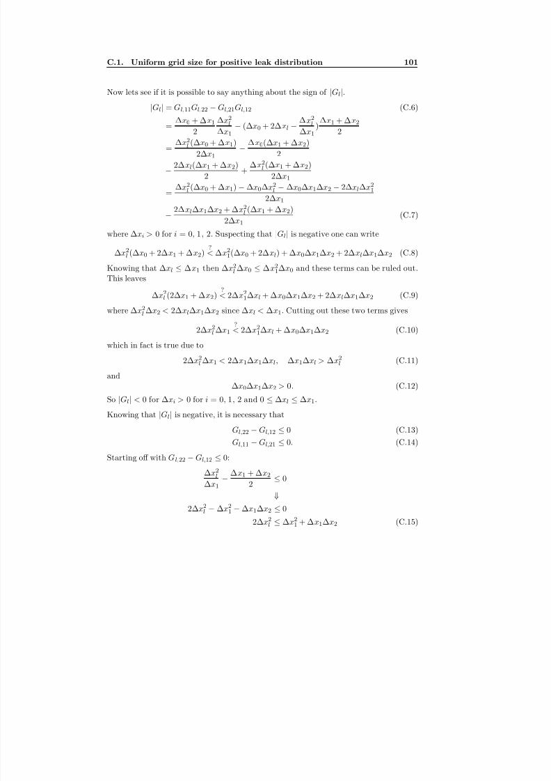
8/18/2019 Advanced Leak Detection using a Nonlinear Observer and OLGA
http://slidepdf.com/reader/full/advanced-leak-detection-using-a-nonlinear-observer-and-olga 109/131
C.1. Uniform grid size for positive leak distribution 101
Now lets see if it is possible to say anything about the sign of |Gl|.
|Gl| = Gl,11Gl,22 − Gl,21Gl,12 (C.6)
= ∆x0 + ∆x1
2
∆x2l
∆x1− (∆x0 + 2∆xl −
∆x2l
∆x1)
∆x1 + ∆x2
2
= ∆x2
l (∆x0 + ∆x1)
2∆x1− ∆x0(∆x1 + ∆x2)
2
− 2∆xl(∆x1 + ∆x2)
2 +
∆x2l (∆x1 + ∆x2)
2∆x1
= ∆x2
l (∆x0 + ∆x1)− ∆x0∆x2l − ∆x0∆x1∆x2 − 2∆xl∆x2
1
2∆x1
− 2∆xl∆x1∆x2 + ∆x2
l (∆x1 + ∆x2)
2∆x1
(C.7)
where ∆xi > 0 for i = 0, 1, 2. Suspecting that |Gl| is negative one can write
∆x2l (∆x0 + 2∆x1 + ∆x2)
?< ∆x2
1(∆x0 + 2∆xl) + ∆x0∆x1∆x2 + 2∆xl∆x1∆x2 (C.8)
Knowing that ∆xl ≤ ∆x1 then ∆x2l ∆x0 ≤ ∆x2
1∆x0 and these terms can be ruled out.This leaves
∆x2l (2∆x1 + ∆x2)
?< 2∆x2
1∆xl + ∆x0∆x1∆x2 + 2∆xl∆x1∆x2 (C.9)
where ∆x2l ∆x2 < 2∆xl∆x1∆x2 since ∆xl < ∆x1. Cutting out these two terms gives
2∆x
2
l ∆x1
?
< 2∆x
2
1∆xl + ∆x0∆x1∆x2 (C.10)which in fact is true due to
2∆x2l ∆x1 < 2∆x1∆x1∆xl, ∆x1∆xl > ∆x2
l (C.11)
and∆x0∆x1∆x2 > 0. (C.12)
So |Gl| < 0 for ∆xi > 0 for i = 0, 1, 2 and 0 ≤ ∆xl ≤ ∆x1.
Knowing that |Gl| is negative, it is necessary that
Gl,22 − Gl,12 ≤ 0 (C.13)
Gl,11 − Gl,21 ≤ 0. (C.14)Starting off with Gl,22 −Gl,12 ≤ 0:
∆x2l
∆x1− ∆x1 + ∆x2
2 ≤ 0
⇓2∆x2
l − ∆x21 − ∆x1∆x2 ≤ 0
2∆x2l ≤ ∆x2
1 + ∆x1∆x2 (C.15)
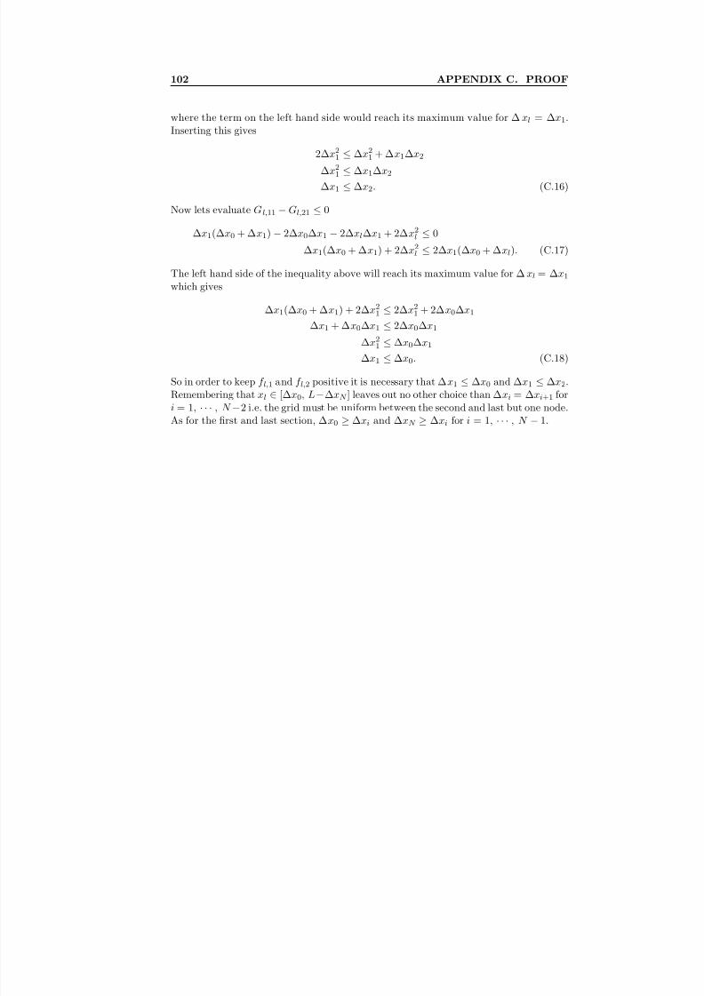
8/18/2019 Advanced Leak Detection using a Nonlinear Observer and OLGA
http://slidepdf.com/reader/full/advanced-leak-detection-using-a-nonlinear-observer-and-olga 110/131
102 APPENDIX C. PROOF
where the term on the left hand side would reach its maximum value for ∆ xl = ∆x1.Inserting this gives
2∆x21 ≤ ∆x2
1 + ∆x1∆x2
∆x21 ≤ ∆x1∆x2
∆x1 ≤ ∆x2. (C.16)
Now lets evaluate Gl,11 −Gl,21 ≤ 0
∆x1(∆x0 + ∆x1) − 2∆x0∆x1 − 2∆xl∆x1 + 2∆x2l ≤ 0
∆x1(∆x0 + ∆x1) + 2∆x2l ≤ 2∆x1(∆x0 + ∆xl). (C.17)
The left hand side of the inequality above will reach its maximum value for ∆ xl = ∆x1
which gives
∆x1(∆x0 + ∆x1) + 2∆x21 ≤ 2∆x2
1 + 2∆x0∆x1
∆x1 + ∆x0∆x1 ≤ 2∆x0∆x1
∆x21 ≤ ∆x0∆x1
∆x1 ≤ ∆x0. (C.18)
So in order to keep f l,1 and f l,2 positive it is necessary that ∆x1 ≤ ∆x0 and ∆x1 ≤ ∆x2.Remembering that xl ∈ [∆x0, L−∆xN ] leaves out no other choice than ∆xi = ∆xi+1 fori = 1, · · · , N −2 i.e. the grid must be uniform between the second and last but one node.
As for the first and last section, ∆x0 ≥ ∆xi and ∆xN ≥ ∆xi for i = 1, · · · , N − 1.

8/18/2019 Advanced Leak Detection using a Nonlinear Observer and OLGA
http://slidepdf.com/reader/full/advanced-leak-detection-using-a-nonlinear-observer-and-olga 111/131
103
Appendix D
Article
The first of the following articles was accepted for oral presentation at the 7th IFACSymposium on Nonlinear Control Systems 22-24 August, 2007 in Pretoria, South Africa.The second one is a draft which will be submitted to SPE Journal.
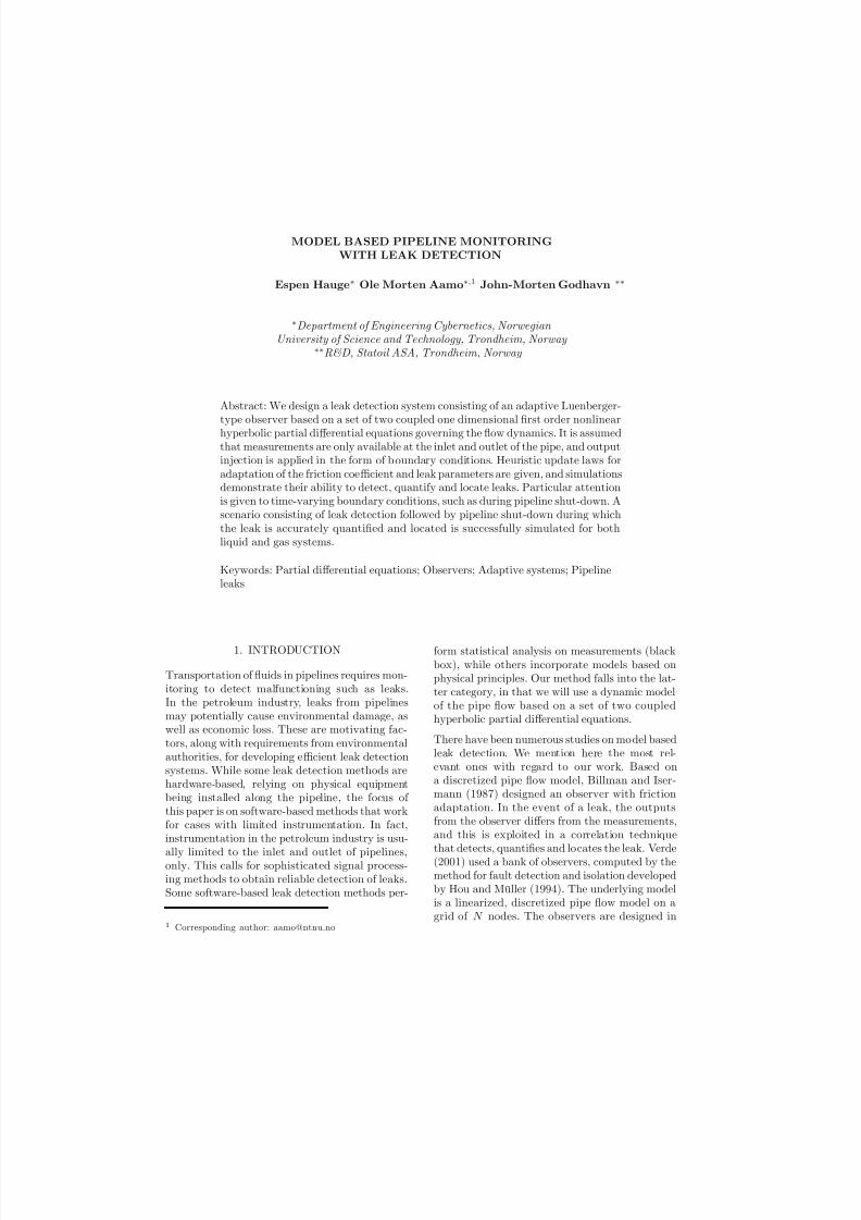
8/18/2019 Advanced Leak Detection using a Nonlinear Observer and OLGA
http://slidepdf.com/reader/full/advanced-leak-detection-using-a-nonlinear-observer-and-olga 112/131
MODEL BASED PIPELINE MONITORING
WITH LEAK DETECTION
Espen Hauge Ole Morten Aamo1 John-Morten Godhavn
Department of Engineering Cybernetics, Norwegian
University of Science and Technology, Trondheim, Norway R&D, Statoil ASA, Trondheim, Norway
Abstract: We design a leak detection system consisting of an adaptive Luenberger-type observer based on a set of two coupled one dimensional first order nonlinearhyperbolic partial di erential equations governing the flow dynamics. It is assumedthat measurements are only available at the inlet and outlet of the pipe, and outputinjection is applied in the form of boundary conditions. Heuristic update laws foradaptation of the friction coecient and leak parameters are given, and simulationsdemonstrate their ability to detect, quantify and locate leaks. Particular attentionis given to time-varying boundary conditions, such as during pipeline shut-down. Ascenario consisting of leak detection followed by pipeline shut-down during whichthe leak is accurately quantified and located is successfully simulated for bothliquid and gas systems.
Keywords: Partial di erential equations; Observers; Adaptive systems; Pipelineleaks
1. INTRODUCTION
Transportation of fluids in pipelines requires mon-itoring to detect malfunctioning such as leaks.In the petroleum industry, leaks from pipelinesmay potentially cause environmental damage, aswell as economic loss. These are motivating fac-tors, along with requirements from environmentalauthorities, for developing ecient leak detectionsystems. While some leak detection methods arehardware-based, relying on physical equipmentbeing installed along the pipeline, the focus of this paper is on software-based methods that workfor cases with limited instrumentation. In fact,instrumentation in the petroleum industry is usu-ally limited to the inlet and outlet of pipelines,
only. This calls for sophisticated signal process-ing methods to obtain reliable detection of leaks.Some software-based leak detection methods per-
1 Corresponding author: [email protected]
form statistical analysis on measurements (blackbox), while others incorporate models based onphysical principles. Our method falls into the lat-
ter category, in that we will use a dynamic modelof the pipe flow based on a set of two coupledhyperbolic partial di erential equations.
There have been numerous studies on model basedleak detection. We mention here the most rel-evant ones with regard to our work. Based ona discretized pipe flow model, Billman and Iser-mann (1987) designed an observer with frictionadaptation. In the event of a leak, the outputsfrom the observer di ers from the measurements,and this is exploited in a correlation techniquethat detects, quantifies and locates the leak. Verde(2001) used a bank of observers, computed by themethod for fault detection and isolation developedby Hou and Müller (1994). The underlying modelis a linearized, discretized pipe flow model on agrid of nodes. The observers are designed in
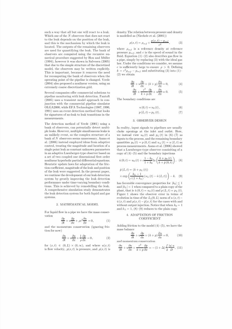
8/18/2019 Advanced Leak Detection using a Nonlinear Observer and OLGA
http://slidepdf.com/reader/full/advanced-leak-detection-using-a-nonlinear-observer-and-olga 113/131
such a way that all but one will react to a leak.Which one of the observers that does not reactto the leak depends on the position of the leak,and this is the mechanism by which the leak is
located. The outputs of the remaining observersare used for quantifying the leak. The bank of observers are computed using the recursive nu-merical procedure suggested by Hou and Müller(1994), however it was shown in Salvesen (2005)that due to the simple structure of the discretizedmodel, the observers may be written explicitly.This is important, because it removes the needfor recomputing the bank of observers when theoperating point of the pipeline is changed. Verde(2004) also proposed a nonlinear version, using anextremely coarse discretization grid.
Several companies o
er commercial solutions topipeline monitoring with leak detection. Fantoft(2005) uses a transient model approach in con-
junction with the commercial pipeline simulatorOLGA2000, while EFA Technologies (1987, 1990,1991) uses an event detection method that looksfor signatures of no-leak to leak transitions in themeasurements.
The detection method of Verde (2001) using abank of observers, can potentially detect multi-ple leaks. However, multiple simultaneous leaks isan unlikely event, so the complex structure of abank of observers seems unnecessary. Aamo etal. (2006) instead employed ideas from adaptivecontrol, treating the magnitude and location of asingle point leak as constant unknown parametersin an adaptive Luenberger-type observer based ona set of two coupled one dimensional first ordernonlinear hyperbolic partial di erential equations.Heuristic update laws for adaptation of the fric-tion coecient, magnitude of the leak and positionof the leak were suggested. In the present paper,we continue the development of our leak detectionsystem by greatly improving the leak detectionperformance under time-varying boundary condi-
tions. This is achieved by remodelling the leak.A comprehensive simulation study demonstratesthe leak detection system for both liquid and gassystems.
2. MATHEMATICAL MODEL
For liquid flow in a pipe we have the mass conser-vation
+
+ 2
= 0 (1)
and the momentum conservation (ignoring fric-tion for now)
+
+
1
= 0 (2)
for ( ) (0 ) × (0), and where ( )is flow velocity, ( ) is pressure, and ( ) is
density. The relation between pressure and densityis modelled as (Nieckele et al. (2001))
( ) = + ( )
2 (3)
where is a reference density at referencepressure , and is the speed of sound in thefluid. Equation (1)—(2) also describes gas flow ina pipe, simply by replacing (3) with the ideal gaslaw. Under the conditions we consider, we assume is suciently large to ensure 0 Defining = 2 and substituting (3) into (1)—(2) we obtain
+
+ ( + )
= 0 (4)
+
2
+
+
= 0 (5)
The boundary conditions are
(0 ) = 0 () (6)
( ) = () (7)
3. OBSERVER DESIGN
In reality, input signals to pipelines are usuallychoke openings at the inlet and outlet. Here,we instead view 0 () and () in (6)—(7) asinputs to the process, and the remaining boundaryquantities 0 () = (0 ) and () = ( ) asprocess measurements. Aamo et al. (2006) showedthat a Luenberger-type observer consisiting of acopy of (4)—(5) and the boundary injections
(0 ) = 0 () + 1 01 + 0
ln
µ + 0 ()
+ ˆ (0 )
¶ (8)
ˆ ( ) = ( + ())
× exp
µ 1
(1 + ) ( () ( ))
¶ (9)
has favorable convergence properties for |0| 1
and || 1 when compared to a plain copy of theplant, that is (0 ) = 0 () and ( ) = ().Figure 1 shows the observer error in terms of evolution in time of the 2(0 ) norm of ( ) ( ) and ( ) ˆ ( ) for the cases with andwithout output injection. Notice that when 0 = 1and = 1, (8)—(9) reduces to the plain copy.
4. ADAPTATION OF FRICTIONCOEFFICIENT
Adding friction to the model (4)—(5), we have themass balance
+ + ( + ) = 0 (10)
and momentum conservation
+
+
2
+
= (1 + )
2
||
(11)
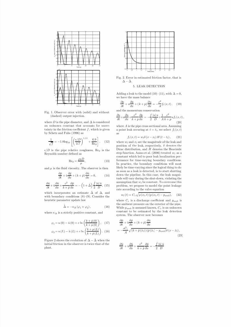
8/18/2019 Advanced Leak Detection using a Nonlinear Observer and OLGA
http://slidepdf.com/reader/full/advanced-leak-detection-using-a-nonlinear-observer-and-olga 114/131
0 5 10 15 20 25 300
0.2
0.4
0.6
0.8
1
1.2
1.4
1.6
1.8
2
Time (s)
L 2
n o r m
o f o b s e r v e
r e r r o r i n u
0 5 10 15 20 25 300
0.2
0.4
0.6
0.8
1
1.2
1.4
1.6
1.8
2x 10
6
Time (s)
L 2
n o
r m
o f o b s e r v e r e r r o r i n p
Fig. 1. Observer error with (solid) and without(dashed) output injection.
where is the pipe diameter, and is consideredan unknown constant that accounts for uncer-tainty in the friction coecient , which is givenby Schetz and Fuhs (1996) as
1
= 18log10
"µ37
¶111
+ 69Re
# (12)
is the pipe relative roughness, Re is theReynolds number defined as
Re =
(13)
and is the fluid viscosity. The observer is then
+
+ ( + ˆ )
= 0 (14)
+
+
2
+ ˆ
= ³1 + ´
2
||
(15)
which incorporates an estimate of andwith boundary conditions (8)—(9). Consider theheuristic parameter update law
˙ = (
1 +
2) (16)
where is a strictly positive constant, and
1
= (0) (0) + ln
µ + ˆ (0)
+ (0)
¶ (17)
2 =
(
) ˆ
(
) +
lnµ + ()
+ ˆ ()
(18)
Figure 2 shows the evolution of when theinitial friction in the observer is twice that of theplant.
0 0.5 1 1.5 2 2.5 3 3.5 4 4.5 5-0.2
0
0.2
0.4
0.6
0.8
1
1.2
Time (min)
E r r o r i n e s t i m a t e o f
Fig. 2. Error in estimated friction factor, that is .
5. LEAK DETECTION
Adding a leak to the model (10)—(11), with = 0we have the mass balance
+
+ ( + )
= 2
( ) (19)
and the momentum conservation
+
+
2
+
=
2
||
+
1
2
+ ( )
(20)where is the pipe cross sectional area. Assuminga point leak occuring at = , we select ( )as
( ) = (
) (
) (21)
where and are the magnitude of the leak andposition of the leak, respectively, denotes theDirac distribution, and denotes the Heavisidestep function. Aamo et al. (2006) treated as aconstant which led to poor leak localization per-formance for time-varying boundary conditions.In practice, the boundary conditions will mostlikely be time-varying since the logical thing to doas soon as a leak is detected, is to start shuttingdown the pipeline. In this case, the leak magni-tude will vary during the shut-down, violating theassumption that be constant. To overcome this
problem, we propose to model the point leakagerate according to the valve equation
() = p
( ) ( ( ) ) (22)
where is a discharge coecient and isthe ambient pressure on the exterior of the pipe.While is assumed known, is an unknownconstant to be estimated by the leak detectionsystem. The observer now becomes
+
+ ( + ˆ )
=
p ( + ˆ ())(ˆ ()
) (
)
(23)
+
+
2
+ ˆ
=
2
||
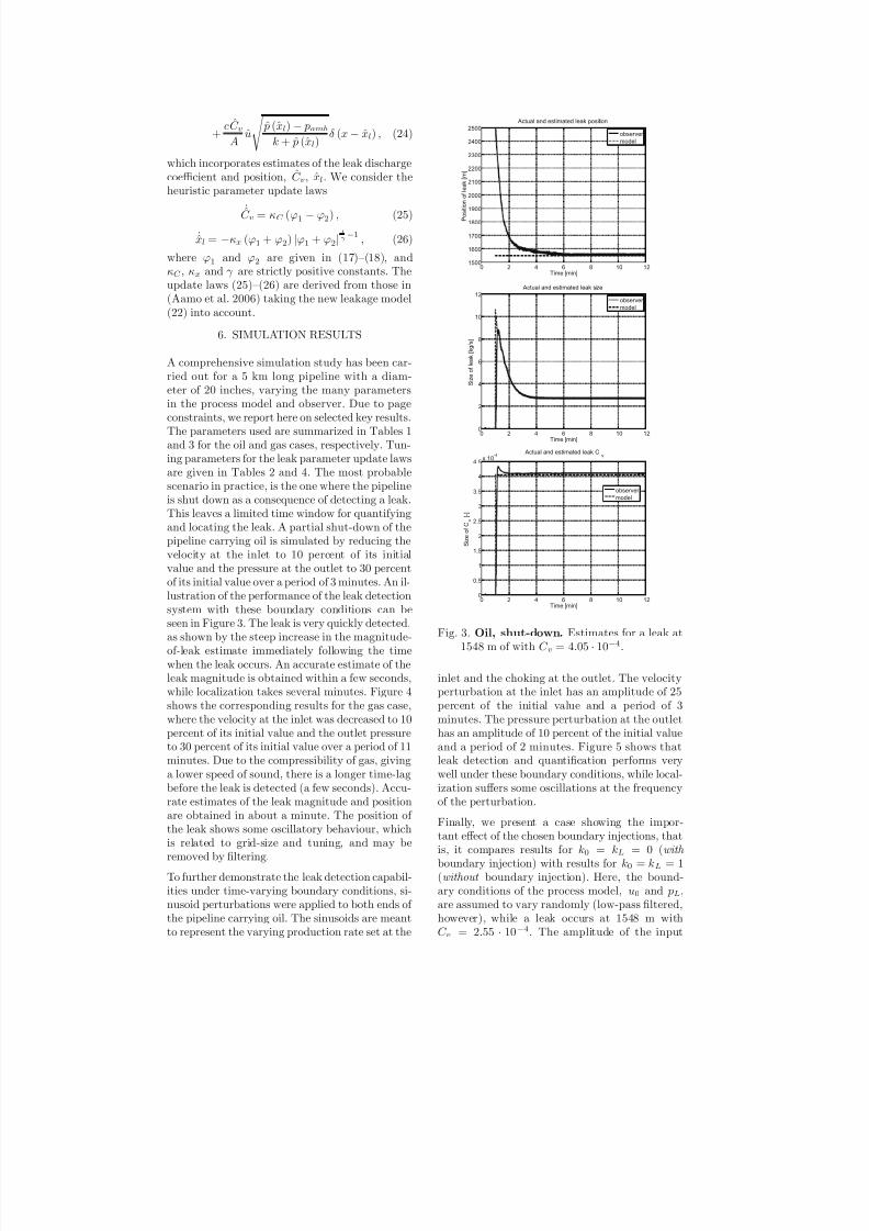
8/18/2019 Advanced Leak Detection using a Nonlinear Observer and OLGA
http://slidepdf.com/reader/full/advanced-leak-detection-using-a-nonlinear-observer-and-olga 115/131
+
s ()
+ ˆ () ( ) (24)
which incorporates estimates of the leak discharge
coecient and position, , . We consider theheuristic parameter update laws
˙ = (
1
2) (25)
˙ = (1
+ 2
) |1
+ 2|1
1
(26)
where 1
and 2
are given in (17)—(18), and and are strictly positive constants. Theupdate laws (25)—(26) are derived from those in(Aamo et al. 2006) taking the new leakage model(22) into account.
6. SIMULATION RESULTS
A comprehensive simulation study has been car-ried out for a 5 km long pipeline with a diam-eter of 20 inches, varying the many parametersin the process model and observer. Due to pageconstraints, we report here on selected key results.The parameters used are summarized in Tables 1and 3 for the oil and gas cases, respectively. Tun-ing parameters for the leak parameter update lawsare given in Tables 2 and 4. The most probablescenario in practice, is the one where the pipelineis shut down as a consequence of detecting a leak.This leaves a limited time window for quantifying
and locating the leak. A partial shut-down of thepipeline carrying oil is simulated by reducing thevelocity at the inlet to 10 percent of its initialvalue and the pressure at the outlet to 30 percentof its initial value over a period of 3 minutes. An il-lustration of the performance of the leak detectionsystem with these boundary conditions can beseen in Figure 3. The leak is very quickly detected,as shown by the steep increase in the magnitude-of-leak estimate immediately following the timewhen the leak occurs. An accurate estimate of theleak magnitude is obtained within a few seconds,while localization takes several minutes. Figure 4
shows the corresponding results for the gas case,where the velocity at the inlet was decreased to 10percent of its initial value and the outlet pressureto 30 percent of its initial value over a period of 11minutes. Due to the compressibility of gas, givinga lower speed of sound, there is a longer time-lagbefore the leak is detected (a few seconds). Accu-rate estimates of the leak magnitude and positionare obtained in about a minute. The position of the leak shows some oscillatory behaviour, whichis related to grid-size and tuning, and may beremoved by filtering.
To further demonstrate the leak detection capabil-ities under time-varying boundary conditions, si-nusoid perturbations were applied to both ends of the pipeline carrying oil. The sinusoids are meantto represent the varying production rate set at the
0 2 4 6 8 10 121500
1600
1700
1800
1900
2000
2100
2200
2300
2400
2500
Actual and estimated leak position
Time [min]
P o s i t i o n o f l e a k [ m
]
observer
model
0 2 4 6 8 10 120
2
4
6
8
10
12
S i z e o f l e a k [ k
g / s ]
Time [min]
Actual and estimated leak size
observer
model
0 2 4 6 8 10 120
0.5
1
1.5
2
2.5
3
3.5
4
4.5x 10
-4 Actual and estimated leak C
v
S i z e o f C
v
[ - ]
Time [min]
observer
model
Fig. 3. Oil, shut-down. Estimates for a leak at1548 m of with = 405 · 104.
inlet and the choking at the outlet. The velocityperturbation at the inlet has an amplitude of 25
percent of the initial value and a period of 3minutes. The pressure perturbation at the outlethas an amplitude of 10 percent of the initial valueand a period of 2 minutes. Figure 5 shows thatleak detection and quantification performs verywell under these boundary conditions, while local-ization su ers some oscillations at the frequencyof the perturbation.
Finally, we present a case showing the impor-tant e ect of the chosen boundary injections, thatis, it compares results for 0 = = 0 (with
boundary injection) with results for 0 = = 1
(without boundary injection). Here, the bound-ary conditions of the process model, 0 and ,are assumed to vary randomly (low-pass filtered,however), while a leak occurs at 1548 m with = 255 · 104. The amplitude of the input
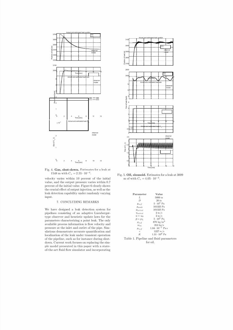
8/18/2019 Advanced Leak Detection using a Nonlinear Observer and OLGA
http://slidepdf.com/reader/full/advanced-leak-detection-using-a-nonlinear-observer-and-olga 116/131
0 2 4 6 8 10 122000
2100
2200
2300
2400
2500
2600
2700
Actual and estimated leak position
Time [min]
P o s i t i o n o f l e a k [ m
]
observer
model
0 2 4 6 8 10 120
1
2
3
4
5
6
Actual and estimated leak size
S i z e o f l e a k [ k
g / s ]
Time [min]
observer
model
0 2 4 6 8 10 120
1
2
x 10-4
Actual and estimated leak Cv
S i z e o f C
v
[ - ]
Time [min]
observer
model
Fig. 4. Gas, shut-down. Estimates for a leak at1548 m with = 255 · 104.
velocity varies within 10 percent of the initialvalue, and the output pressure varies within 0.7percent of the initial value. Figure 6 clearly showsthe crucial e ect of output injection, as well as theleak detection capability under randomly varyinginput.
7. CONCLUDING REMARKS
We have designed a leak detection system forpipelines consisting of an adaptive Luenberger-type observer and heuristic update laws for theparameters characterizing a point leak. The onlyavailable process information is flow velocity andpressure at the inlet and outlet of the pipe. Sim-ulations demonstrate accurate quantification and
localization of the leak under transient operationof the pipeline, such as for instance during shut-down. Current work focuses on replacing the sim-ple model presented in this paper with a state-of-the-art fluid flow simulator and incorporating
0 2 4 6 8 10 122500
2600
2700
2800
2900
3000
3100
Actual and estimated leak position
Time [min]
P o s i t i o n o f l e a k [ m ]
observer
model
0 2 4 6 8 10 120
2
4
6
8
10
12
Actual and estimated leak size
S i z e o f l e a k [ k g / s ]
Time [min]
observer
model
0 2 4 6 8 10 120
0.5
1
1.5
2
2.5
3
3.5
4
4.5x 10
-4 Actual and estimated leak C
v
S i z e o f C
v
[ - ]
Time [min]
observer
model
Fig. 5. Oil, sinusoid. Estimates for a leak at 3009m of with = 405 · 104.
Parameter Value
5000 m 20 in
5 · 105 Pa
101325 Pa initia l 101325 Painitia l 2 m /s = 0 2 m /s¯ = 5 · 10
5 Pa 870 kg/m3
353 kg/s 104 · 10
1 Pa·s
1227 m /s
131 ·
10
9
PaTable 1. Pipeline and fluid parameters
for oil.
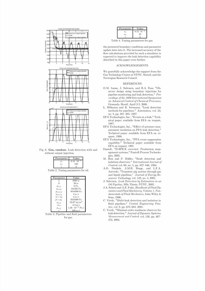
8/18/2019 Advanced Leak Detection using a Nonlinear Observer and OLGA
http://slidepdf.com/reader/full/advanced-leak-detection-using-a-nonlinear-observer-and-olga 117/131
0 2 4 6 8 10 12800
1000
1200
1400
1600
1800
2000
2200
2400
2600
Actual and estimated leak position
Time [min]
P o s i t i o n o f l e a k [ m
]
observer w/ output injection
model
observer w/o output injection
0 2 4 6 8 10 120
2
4
6
8
10
12
14
Actual and estimated leak size
S i z e o f l e a k [ k g / s ]
Time [min]
observer w/ output injection
model
observer w/o output injection
0 2 4 6 8 10 120
1
2
3
4
5
6x 10
-4 Actual and estimated leak C
v
S i z e o f C
v
[ - ]
Time [min]
observer w/ output injection
model
observer w/o output injection
Fig. 6. Gas, random. Leak detection with andwithout output injection.
Pa ra me te r Va lu e
812 · 104
100
4
Table 2. Tuning parameters for oil.
Parameter Value
5000 m 20 in
0 Pa 101325 Pa initia l 5016390 Painitia l 4 m /s = 0 4 m /s¯ = 5016390 Pa 5267 kg/m3
43 kg/s
120 · 105 Pa
·s
308 m /s
Table 3. Pipeline and fluid parametersfor gas.
Pa ra me te r Va lu e
812 · 104
35
4
Table 4. Tuning parameters for gas.
the presented boundary conditions and parameterupdate laws into it. The increased accuracy of theflow calculations provided by such a simulator isexpected to improve the leak detection capabilitydescribed in this paper even further.
ACKNOWLEDGEMENTS
We gratefully acknowledge the support from theGas Technology Center at NTNU, Statoil, and theNorwegian Research Council.
REFERENCES
O.M. Aamo, J. Salvesen, and B.A. Foss, "Ob-server design using boundary injections forpipeline monitoring and leak detection," Pro-
ceedings of the 2006 International Symposium
on Advanced Control of Chemical Processes,
Gramado, Brazil, April 2-5, 2006.L. Billmann and R. Isermann, "Leak detection
methods for pipelines," Automatica , vol. 23,no. 3, pp. 381—385, 1987.
EFA Technologies, Inc., "Events at a leak," Tech-nical paper available from EFA on request,
1987.EFA Technologies, Inc., "E ect of pressure mea-surement resolution on PPA leak detection,"Technical paper available from EFA on re-quest, 1990.
EFA Technologies, Inc., "PPA event suppressioncapability," Technical paper available fromEFA on request, 1991.
Fantoft, "D-SPICE overview: Production man-agement systems," Fantoft Process Technolo-gies, 2005.
M. Hou and P. Müller, "Fault detection andisolation observers," International Journal of
Control , vol. 60, no. 5, pp. 827—846, 1994.A.O. Nieckele, A.M.B. Brage, and L.F.A.Azevedo, "Transient pig motion through gasand liquid pipelines," Journal of Energy Re-
sources Technology , vol. 123, no. 4, 2001.J. Salvesen, Leak Detection by Estimation in an
Oil Pipeline , MSc Thesis, NTNU, 2005.J.A. Schetz and A.E. Fuhs, Handbook of Fluid Dy-
namics and Fluid Machinery, Volume 1, Fun-
damentals of Fluid Mechanics , John Wiley &Sons, 1996.
C. Verde, "Multi-leak detection and isolation influid pipelines," Control Engineering Prac-
tice , vol. 9, pp. 673—682, 2001.C. Verde, "Minimal order nonlinear observer for
leak detection," Journal of Dynamic Systems,
Measurement and Control , vol. 126, pp. 467—472, 2004.
8/18/2019 Advanced Leak Detection using a Nonlinear Observer and OLGA
http://slidepdf.com/reader/full/advanced-leak-detection-using-a-nonlinear-observer-and-olga 118/131
Abstract
An adaptive Luenberger-type observer with the
purpose of locating and quantifying leakages is
presented. The observer only needs measurements
of velocity and temperature at the inlet and pressure
at the outlet to function. The beneficial effect of
output injection in form of boundary conditions is
used to ensure fast convergence of the observer
error. Depending only on measurements from inlet
and outlet makes it possible to use OLGA, which is
a state of the art computational fluid dynamics
simulator, to govern the one-phase fluid flow of the
observer. The observer is tested with both a straight,
horizontal pipeline and an actual, long pipeline with
inclinations, and both simulations with oil and gas
are carried out. In order to cope with modelling
errors and biased measurements, estimation of
roughness in the monitored pipeline is introduced.
1 Introduction
Leak detection based on dynamic modelling is a
propitious approach in the special field of leak
quantification and location. This article documents
one of the first steps toward a new method of
pipeline monitoring. A state of the art multiphase
simulator is manipulated through Matlab to work as
an adaptive Luenberger-type observer which uses
measurements from the supervised pipeline as well
as internal measurements. Since the only
measurements fed into the observer are pressure
from the outlet and velocity and temperature from
the inlet, which in most cases already are available,
the method can be used with most existing pipelines
without extra instrumentation. Also, the
computational fluid dynamics simulator, which is
the backbone of the observer, is a widely used one,
SPE Paper Number ?
Advanced leak detection in oil and gas pipelines using a nonlinear observer and OLGAmodelsEspen Hauge, Ole Morten Aamo, and John-Morten Godhavn, Norwegian University of Science and Technology
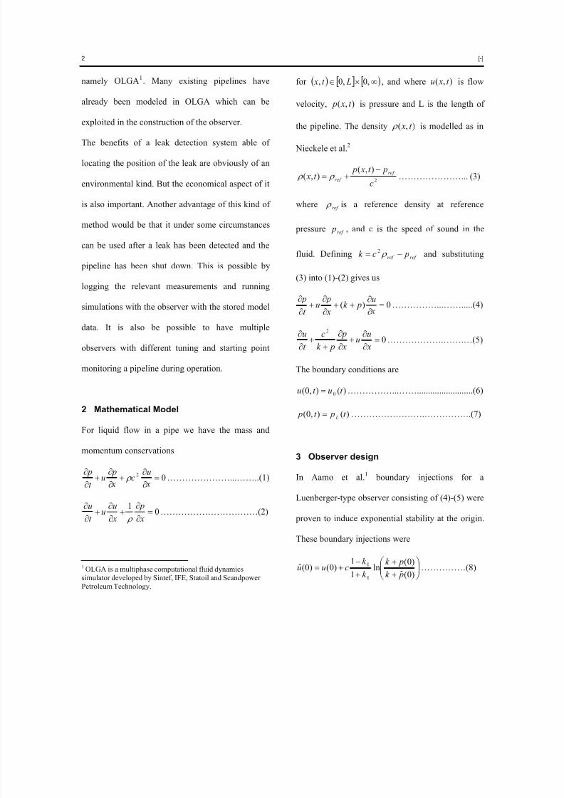
8/18/2019 Advanced Leak Detection using a Nonlinear Observer and OLGA
http://slidepdf.com/reader/full/advanced-leak-detection-using-a-nonlinear-observer-and-olga 119/131
2 [-]
namely OLGA1. Many existing pipelines have
already been modeled in OLGA which can be
exploited in the construction of the observer.
The benefits of a leak detection system able of
locating the position of the leak are obviously of an
environmental kind. But the economical aspect of it
is also important. Another advantage of this kind of
method would be that it under some circumstances
can be used after a leak has been detected and the
pipeline has been shut down. This is possible by
logging the relevant measurements and running
simulations with the observer with the stored model
data. It is also be possible to have multiple
observers with different tuning and starting point
monitoring a pipeline during operation.
2 Mathematical Model
For liquid flow in a pipe we have the mass and
momentum conservations
02
uc
pu
t
p …………………...……..(1)
01
x
p
x
uu
t
u
……………………………(2)
1 OLGA is a multiphase computational fluid dynamicssimulator developed by Sintef, IFE, Statoil and Scandpower
Petroleum Technology.
for ,0,0, Lt x , and where is flow
velocity, is pressure and L is the length of
the pipeline. The density
),( t xu
),( t x p
),( t x is modelled as in
Nieckele et al.2
2
),(),(
c
pt x pt x
ref
ref
…………………... (3)
where ref is a reference density at reference
pressure , and c is the speed of sound in the
fluid. Defining and substituting
(3) into (1)-(2) gives us
ref p
ref ref pck 2
0)(
u pk
x
pu
t
p……………...…….....(4)
0
2
x
u
u x
p
pk
c
t
u
……………….…….…(5)
The boundary conditions are
)(),0( 0 t ut u ……………...…….........................(6)
)(),0( t pt p L …………………….…………….(7)
3 Observer design
In Aamo et al.1 boundary injections for a
Luenberger-type observer consisting of (4)-(5) were
proven to induce exponential stability at the origin.
These boundary injections were
)0(ˆ
)0(
ln1
1
)0()0(ˆ0
0
pk
pk
k
k
cuu ……………(8)
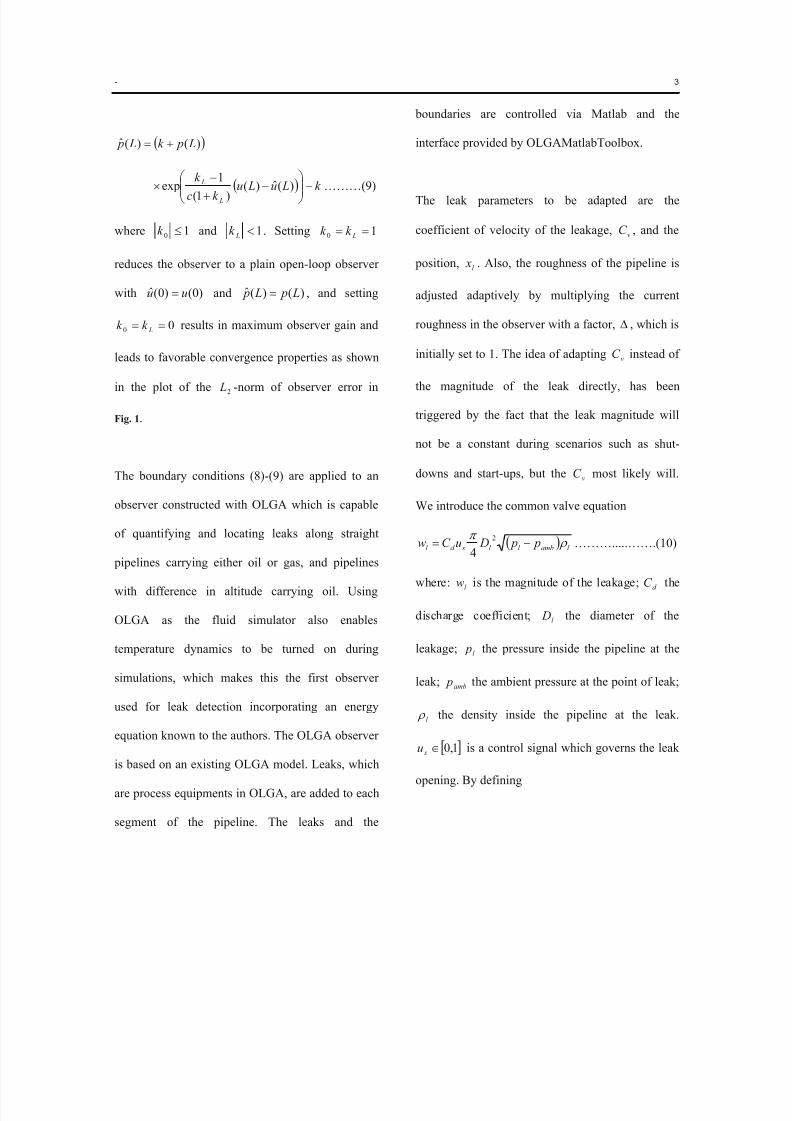
8/18/2019 Advanced Leak Detection using a Nonlinear Observer and OLGA
http://slidepdf.com/reader/full/advanced-leak-detection-using-a-nonlinear-observer-and-olga 120/131
- 3
)()(ˆ L pk L p
k Lu Luk c
k
L
L
)(ˆ)(
)1(
1exp ………(9)
where 10 k and 1 Lk . Setting 10 Lk k
reduces the observer to a plain open-loop observer
with and , and setting
results in maximum observer gain and
leads to favorable convergence properties as shown
in the plot of the -norm of observer error in
)0()0(ˆ uu )()(ˆ L p L p
00 Lk k
2 L
Fig. 1.
The boundary conditions (8)-(9) are applied to an
observer constructed with OLGA which is capable
of quantifying and locating leaks along straight
pipelines carrying either oil or gas, and pipelines
with difference in altitude carrying oil. Using
OLGA as the fluid simulator also enables
temperature dynamics to be turned on during
simulations, which makes this the first observer
used for leak detection incorporating an energy
equation known to the authors. The OLGA observer
is based on an existing OLGA model. Leaks, which
are process equipments in OLGA, are added to each
boundaries are controlled via Matlab and the
interface provided by OLGAMatlabToolbox.
segment of the pipeline. The leaks and the
he leak parameters to be adapted are theT
coefficient of velocity of the leakage, vC , and the
position, l x . Also, the roughness of the pipeline is
adjusted adaptively by multiplying the current
roughness in the observer with a factor, , which is
initially set to 1. The idea of adapting C instead of
the magnitude of the leak directly, has been
triggered by the fact that the leak magnitude will
not be a constant during scenarios such as shut-
downs and start-ups, but the vC most likely will.
We introduce the common valve equation
v
l ambl l sd l p p DuC w
2
……….....…4
….(10)
where: is the magnitude of the leakage; the
e
l w d C
discharg coefficient; l D the diameter of the
leakage; l p the pressure inside the pipeline at the
leak; amb p he ambient pressure at the point of leak;
l
t
the density inside the pipeline at the leak.
1,0 su is a control signal which governs the leak
By definingopening.
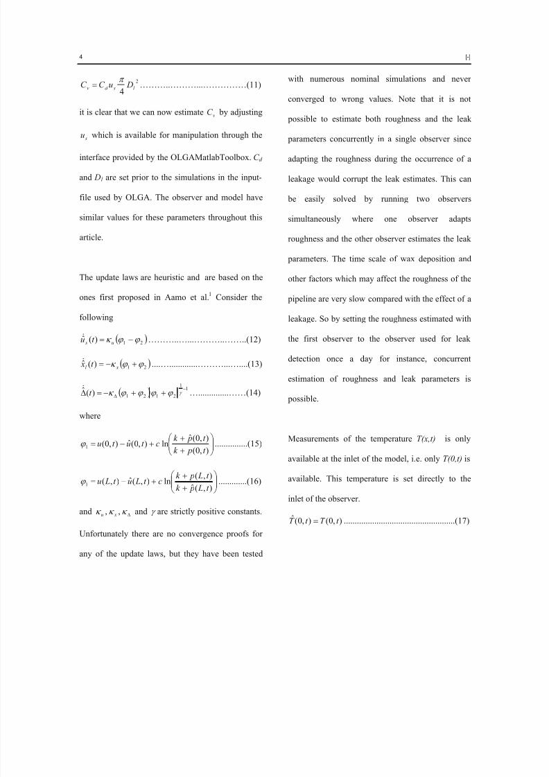
8/18/2019 Advanced Leak Detection using a Nonlinear Observer and OLGA
http://slidepdf.com/reader/full/advanced-leak-detection-using-a-nonlinear-observer-and-olga 121/131
4 [-]
2
4 l sd v DuC C
………..………...……………(11)
it is clear that we can now estimate by adjusting
which is available for manipulation through the
interface provided by the OLGAMatlabToolbox. C
vC
su
d
and Dl are set prior to the simulations in the input-
file used by OLGA. The observer and model have
similar values for these parameters throughout this
article.
The update laws are heuristic and are based on the
ones first proposed in Aamo et al.1 Consider the
following
21)(ˆ u s t u
………..…...………..……..(12)
21)(ˆ xl t x ....….............………...…....(13)
1
1
2121)(ˆ
t
…..............……(14)
where
),0(
),0(ˆln),0(ˆ),0(1
t pk
t pk ct ut u ...............(15)
),(ˆ
),(ln),(ˆ),(1
t L pk
t L pk ct Lut Lu .............(16)
and ,, xu and are strictly positive constants.
Unfortunately there are no convergence proofs for
any of the update laws, but they have been tested
with numerous nominal simulations and never
converged to wrong values. Note that it is not
possible to estimate both roughness and the leak
parameters concurrently in a single observer since
adapting the roughness during the occurrence of a
leakage would corrupt the leak estimates. This can
be easily solved by running two observers
simultaneously where one observer adapts
roughness and the other observer estimates the leak
parameters. The time scale of wax deposition and
other factors which may affect the roughness of the
pipeline are very slow compared with the effect of a
leakage. So by setting the roughness estimated with
the first observer to the observer used for leak
detection once a day for instance, concurrent
estimation of roughness and leak parameters is
possible.
Measurements of the temperature T(x,t) is only
available at the inlet of the model, i.e. only T(0,t) is
available. This temperature is set directly to the
inlet of the observer.
),0(),0(ˆ t T t T ...................................................(17)
8/18/2019 Advanced Leak Detection using a Nonlinear Observer and OLGA
http://slidepdf.com/reader/full/advanced-leak-detection-using-a-nonlinear-observer-and-olga 122/131
- 5
4 Simulation results
A comprehensive simulation study has been
conducted as part of a Master thesis at the
Norwegian University of Science and Technology
(NTNU). A few chosen results from this thesis are
presented in this section. The observers are in all
cases initialized with the same values as the model
and temperature dynamics is turned on during all
simulations.
In Table 1 a straight, horizontal pipeline is defined,
and the tuning of the corresponding observer is
presented in Table 4. This observer is set to monitor
the pipeline with the boundaries seen in Fig. 2. The
leak occurs after one minute, simultaneously as the
boundaries start to vary. This is supposed to
resemble the effect which can be caused by
controlling chokes at inlet and outlet. Fig. 4 shows
the estimated leak parameters. The effect of the
sinusoidal boundary conditions is clearly visible,
and none of the estimates converge to a certain
value. But still it is possible to narrow down to an
area where the leak has occurred. Estimation of the
roughness was conducted prior to the leakage and
then turned off so it would not interfere with the
estimates of the leak parameters. A plot of the
estimated roughness for this case can be seen in
Fig. 3.
In Table 2 parameters for a straight, horizontal
pipeline carrying gas are presented. An OLGA
observer was constructed to monitor this model and
its tuning can be seen in Table 5. The estimates in
Fig. 5 show that it is possible to quantify and locate
a leakage during stationary gas flow. The estimated
friction is presented in Fig. 6.
In Fig. 7 the boundaries for a model of an actual,
long pipeline during start-up are showed. The
profile for this pipeline is plotted in Fig. 10. The
parameters for this pipeline are presented in Table 3
and the tuning of the corresponding observer can be
seen in Table 6. After 3 minutes a leak occurs
which is detected by the observer. The estimated
leak parameters are plotted in Fig. 8. Notice that the
estimated C v is lower than the actual. This is due to
a modification done in the observer monitoring
pipelines with inclinations. Instead of having
ambient pressure in the observer at the position of
the leak depending on the depth, it is set to 1 atm
8/18/2019 Advanced Leak Detection using a Nonlinear Observer and OLGA
http://slidepdf.com/reader/full/advanced-leak-detection-using-a-nonlinear-observer-and-olga 123/131
6 [-]
even though the pipeline reaches depths down to
510 m. This modification has shown to be
successful since the adaption of is smoother.
This can be explained by considering the following:
while adapting , is moving along the pipeline,
possibly through an inclined part. With
backpressure at each leak depending on the depth,
the differential pressure over the leaks can vary
vastly from one segment to another, which again
will cause to fluctuate when passes through.
This opposes the idea of estimating a constant
parameter and is coped with by defining the
ambient pressure in the observer as 1 atm at every
leak.
vC ˆ
vC ˆl x
vC ˆl x
The last case in this article involves biased
measurements from the model and stationary
boundary conditions. The pressure measurements
from the inlet and outlet of the model are added a
bias of -0.10 bar each. This error is coped with by
estimating the roughness prior to the leakage, which
magnitude is only 0.20 % of the mass rate at the
inlet. The pipeline and tuning parameters are
presented in Table 3 and Table 6, respectively. The
plot of estimates with and without adaption of
roughness can be seen in Fig. 9.
5 Conclusions
The adaptive Luenberger-type observer presented in
this article uses OLGA as its computational fluid
dynamics simulator which is a state of the art
simulator for one-, two- and three-phase flow. The
OLGA observer is manipulated through Matlab
which make it possible to make use of output
injection in form of boundary conditions, control
the magnitude and position of the estimated leakage
and adapt roughness to compensate for model errors
and biased measurements. The OLGA observer has
numerous advantages over its predecessor, i.e. the
observer constructed with Matlab in Aamo et al.1,
among which the incorporation of temperature
dynamics, the support for pipelines with difference
in altitude and that it is widely used by oil
companies are the most important ones. It has also
proved to work with time-varying boundary
conditions for pipelines carrying oil.
8/18/2019 Advanced Leak Detection using a Nonlinear Observer and OLGA
http://slidepdf.com/reader/full/advanced-leak-detection-using-a-nonlinear-observer-and-olga 124/131
- 7
Acknowledgements
We gratefully acknowledge the support from the
Gas Technology Center at NTNU, Statoil, and the
Norwegian Research Council.
Nomenclature
c Speed of sound in the fluid, [L/t], m/s
C d Discharge coefficient of leakage, [-]
C v Valve constant for leak in the model, [L2],
m2
vC ˆ Valve constant for leak in the observer,
[L2], m
2
Dl Diameter of leak opening, [L], m
Estimated factor which is used for adaption
of roughness, [-]
Tuning coefficient in update law for leak
position, [-]
k 0 Tuning constant for the output injection at
the outlet, [-]
k L Tuning constant for the output injection at
the inlet, [-]
Tuning coefficient in update law for
roughness, [-]
u Tuning coefficient in update law for leak
magnitude, [-]
x Tuning coefficient in update law for leak
position, [-]
L Length of pipeline, [L], m
p Pressure in the model, [m/Lt2], bara
p Pressure in the observer, [m/Lt2], bara
pamb Ambient pressure, [m/Lt2], atm
Density of the fluid in the model, [m/L3],
kg/m3
l Density of the fluid at the point of leak
[m/L3], kg/m
3
T Temperature in model, [T], K
T Temperature in observer, [T], K
u Velocity of fluid in the model, [L/t], m/s
u Velocity of fluid in the observer, [L/t], m/s
u s Control signal used to govern the leak
opening in the model, [-]
su Estimated control signal used to govern the
leak opening in the observer, [-]
wl Magnitude of leak, [m/t], kg/s
xl Actual leak position, [L], m
l x Estimated leak position, [L], m
8/18/2019 Advanced Leak Detection using a Nonlinear Observer and OLGA
http://slidepdf.com/reader/full/advanced-leak-detection-using-a-nonlinear-observer-and-olga 125/131
8 [-]
References
1. Aamo, O.M., Salvesen, J. and Foss, B.A.:
Observer design using boundary injections for
pipeline monitoring and leak detection,
presented at the Adchem 2006 conference,
Gamado, Brazil, April 2-5, 2006.
2. Nieckele, A.O., Brage, A.M.B. and Azevedo
L.F.A.: Transient pig motion through gas and
liquid pipelines, Journal of Energy Resources
Technology, vol. 123. no. 4, 2001.
SI Metric Conversion Factors
bar × 1.0* E+05 = Pa
ft × 3.048* E-01 = m
ft2
× 9.290 304* E-02 = m2
ft3
× 2.831 685 E-02 = m3
°F (°F+459.67)/1.8 = K
lbm × 4.535 924 E-01 = kg
*Conversion factor is exact.
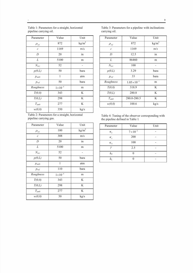
8/18/2019 Advanced Leak Detection using a Nonlinear Observer and OLGA
http://slidepdf.com/reader/full/advanced-leak-detection-using-a-nonlinear-observer-and-olga 126/131
- 9
Table 1: Parameters for a straight, horizontal
pipeline carrying oil.
Parameter Value Unit
ref 872 kg/m3
c 1169 m/s
D 20 in
L 5100 m
N sec 52 -
p(0,L) 50 bara
pamb 1 atm pref 50 bara
Roughness 5101 m
T(0,0) 343 K
T(0,L) 298 K
T amb 277 K
w(0,0) 350 kg/s
Table 2: Parameters for a straight, horizontal pipeline carrying gas.
Parameter Value Unit
ref 100 kg/m3
c 308 m/s
D 20 in
L 5100 m
N sec 52 -
p(0,L) 50 bara
pamb 1 atm
pref 110 bara
Roughness 5101 m
T(0,0) 343 K
T(0,L) 298 K
T amb 277 K
w(0,0) 50 kg/s
Table 3: Parameters for a pipeline with inclinations
carrying oil.
Parameter Value Unit
ref 872 kg/m3
c 1169 m/s
D 12.5 in
L 86460 m
N sec 100 -
p(0,L) 3.29 bara
pref 33 bara Roughness 31005.1 m
T(0,0) 318.9 K
T(0,L) 280.8 K
T amb 280.0-280.5 K
w(0,0) 100.6 kg/s
Table 4: Tuning of the observer corresponding withthe pipeline defined in Table 1.
Parameter Value Unit
u 3107 -
x 200 -
100 -
2.5 -
k 0 0 -
k L 0 -
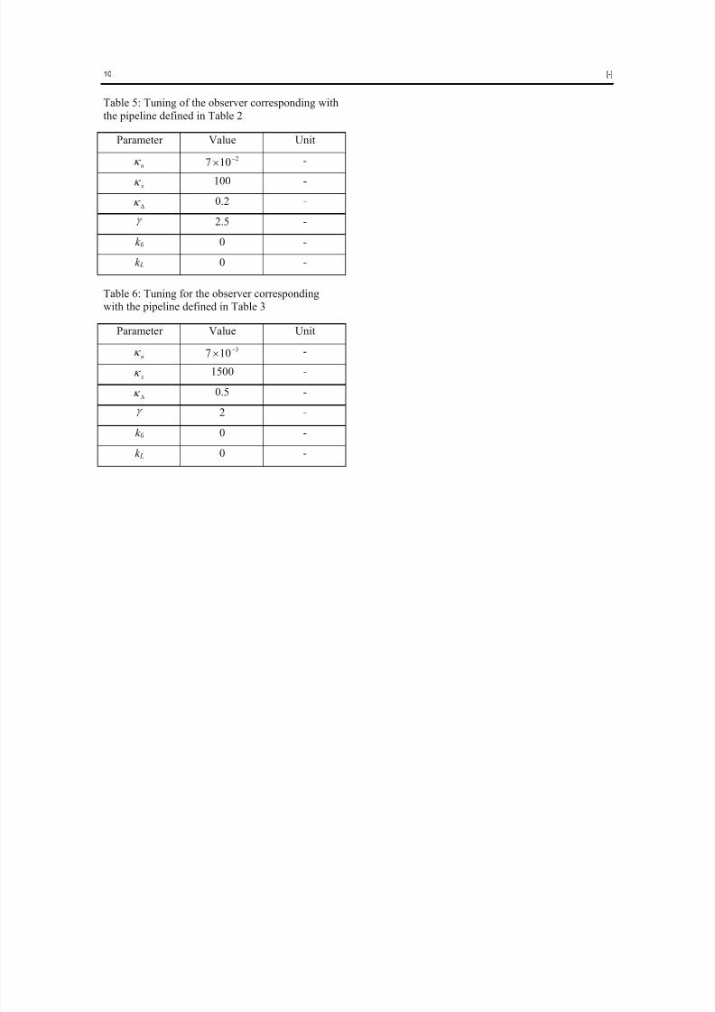
8/18/2019 Advanced Leak Detection using a Nonlinear Observer and OLGA
http://slidepdf.com/reader/full/advanced-leak-detection-using-a-nonlinear-observer-and-olga 127/131
10 [-]
Table 5: Tuning of the observer corresponding with
the pipeline defined in Table 2
Parameter Value Unit
u 2107 -
x 100 -
0.2 -
2.5 -
k 0 0 -
k L 0 -
Table 6: Tuning for the observer correspondingwith the pipeline defined in Table 3
Parameter Value Unit
u 3107 -
x 1500 -
0.5 -
2 -
k 0 0 -
k L 0 -
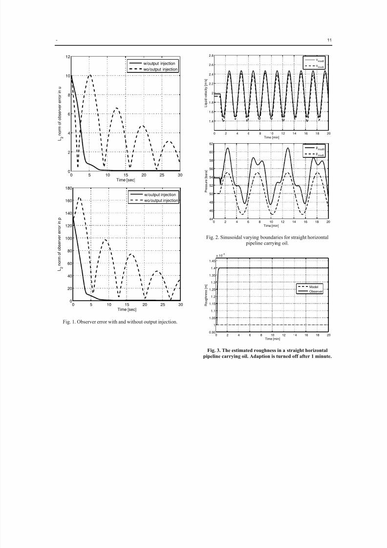
8/18/2019 Advanced Leak Detection using a Nonlinear Observer and OLGA
http://slidepdf.com/reader/full/advanced-leak-detection-using-a-nonlinear-observer-and-olga 128/131
- 11
0 5 10 15 20 25 300
2
4
6
8
10
12
Time [sec]
L 2 n o r m o
f o b s e r v e r e r r o r i n u
w/output injection
wo/output injection
0 5 10 15 20 25 300
20
40
60
80
100
120
140
160
180
Time [sec]
L 2 n o r m o f o b s e r v e r e r r o r i n p
w/output injection
wo/output injection
Fig. 1. Observer error with and without output injection.
0 2 4 6 8 10 12 14 16 18 20
1.4
1.6
1.8
2
2.2
2.4
2.6
2.8
Time [min]
L i q u i d v e l o c i t y [ m / s ]
umod0
umodL
0 2 4 6 8 10 12 14 16 18 2044
46
48
50
52
54
56
58
60
62
Time [min]
P r e s s u r e [ b a r a ]
pmod0
pmodL
Fig. 2. Sinusoidal varying boundaries for straight horizontal pipeline carrying oil.
0 2 4 6 8 10 12 14 16 18 200.95
1
1.05
1.1
1.15
1.2
1.25
1.3
1.35
1.4
1.45
x 10−5
Time [min]
R o u g h n e s s [ m ]
Model
Observer
Fig. 3. The estimated roughness in a straight horizontal
pipeline carrying oil. Adaption is turned off after 1 minute.
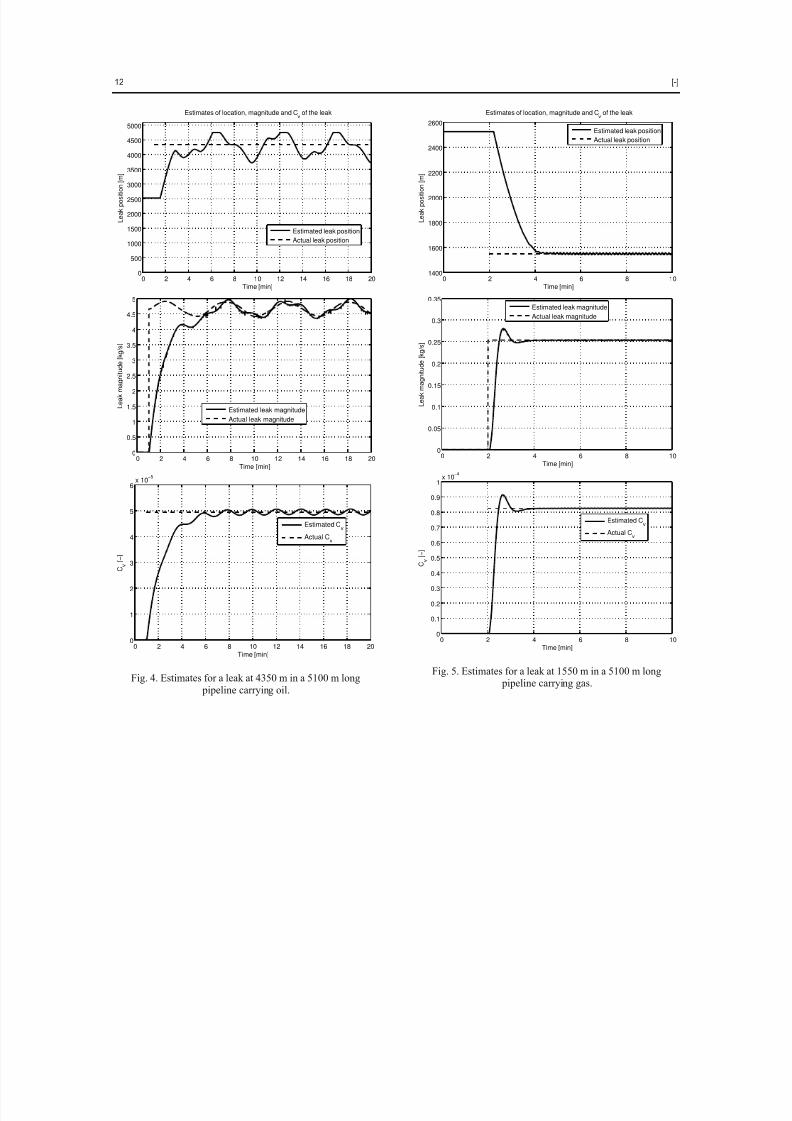
8/18/2019 Advanced Leak Detection using a Nonlinear Observer and OLGA
http://slidepdf.com/reader/full/advanced-leak-detection-using-a-nonlinear-observer-and-olga 129/131
12 [-]
0 2 4 6 8 10 12 14 16 18 200
500
1000
1500
2000
2500
3000
3500
4000
4500
5000
Estimates of location, magnitude and Cv of the leak
Time [min]
L e a k p o s i t i o n [ m ]
Estimated leak position
Actual leak position
0 2 4 6 8 10 12 14 16 18 200
0.5
1
1.5
2
2.5
3
3.5
4
4.5
5
Time [min]
L e a k m a g n i t u d e [ k g / s ]
Estimated leak magnitude
Actual leak magnitude
0 2 4 6 8 10 12 14 16 18 200
1
2
3
4
5
6x 10⁻⁵
Time [min]
C v
[ − ]
Estimated Cv
Actual Cv
Fig. 4. Estimates for a leak at 4350 m in a 5100 m long
pipeline carrying oil.
0 2 4 6 8 101400
1600
1800
2000
2200
2400
2600
Estimates of location, magnitude and Cv of the leak
Time [min]
L e a k p o s i t i o n [ m ]
Estimated leak position
Actual leak position
0 2 4 6 8 100
0.05
0.1
0.15
0.2
0.25
0.3
0.35
Time [min]
L e a k m a g n i t u d e [ k g / s ]
Estimated leak magnitude
Actual leak magnitude
0 2 4 6 8 100
0.1
0.2
0.3
0.4
0.5
0.6
0.7
0.8
0.9
1 x 10
−4
Time [min]
C v
[ − ]
Estimated Cv
Actual Cv
Fig. 5. Estimates for a leak at 1550 m in a 5100 m long pipeline carrying gas.
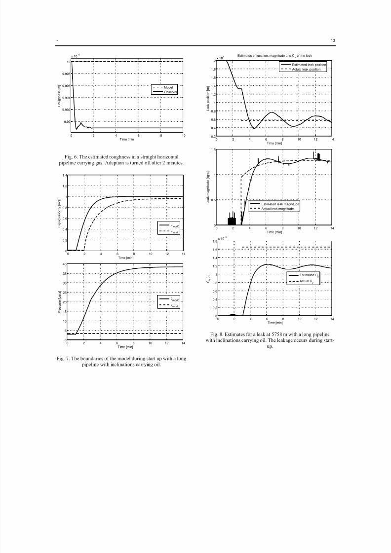
8/18/2019 Advanced Leak Detection using a Nonlinear Observer and OLGA
http://slidepdf.com/reader/full/advanced-leak-detection-using-a-nonlinear-observer-and-olga 130/131
- 13
0 2 4 6 8 10
9.99
9.992
9.994
9.996
9.998
10
x 10−6
Time [min]
R o u g h n e s s [ m ]
Model
Observer
Fig. 6. The estimated roughness in a straight horizontal pipeline carrying gas. Adaption is turned off after 2 minutes.
0 2 4 6 8 10 12 140
0.2
0.4
0.6
0.8
1
1.2
1.4
Time [min]
L i q u i d v e l o c i t y [ m / s ]
umod0
umodL
0 2 4 6 8 10 12 140
5
10
15
20
25
30
35
40
Time [min]
P r e s s u r e [ b a r a ]
pmod0
pmodL
Fig. 7. The boundaries of the model during start up with a long
pipeline with inclinations carrying oil.
0 2 4 6 8 10 12 140.2
0.4
0.6
0.8
1
1.2
1.4
1.6
1.8
2x 10
4 Estimates of location, magnitude and Cv of the leak
Time [min]
L e a k p o s i t i o n [ m ]
Estimated leak position
Actual leak position
0 2 4 6 8 10 12 140
0.5
1
1.5
Time [min]
L e a k m a g n i t u d e [ k g / s ]
Estimated leak magnitude
Actual leak magnitude
0 2 4 6 8 10 12 140
0.2
0.4
0.6
0.8
1
1.2
1.4
1.6
1.8x 10
−5
Time [min]
C v
[ − ] Estimated C
v
Actual Cv
Fig. 8. Estimates for a leak at 5758 m with a long pipelinewith inclinations carrying oil. The leakage occurs during start-
up.
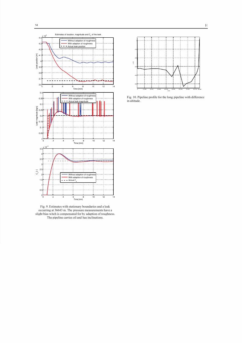
8/18/2019 Advanced Leak Detection using a Nonlinear Observer and OLGA
http://slidepdf.com/reader/full/advanced-leak-detection-using-a-nonlinear-observer-and-olga 131/131
14 [-]
0 2 4 6 8 10 12 143.6
3.7
3.8
3.9
4
4.1
4.2
4.3
4.4x 10
4 Estimates of location, magnitude and Cv of the leak
Time [min]
L e a k p o s i t i o n [ m ]
Without adaption of roughness
With adaption of roughness
Actual leak position
0 2 4 6 8 10 12 140
0.05
0.1
0.15
0.2
0.25
0.3
0.35
0.4
Time [min]
L e a k m a g n i t u d e [ k g / s ]
Without adaption of roughness
With adaption of roughness
Actual leak magnitude
3
3.5
4
4.5x 10⁻⁶
0 10 000 20 000 30 000 40 000 50 000 60 000 70 000 80 000 86 460
−500
−400
−300
−200
−100
0
x [m]
y [ m ]
Fig. 10. Pipeline profile for the long pipeline with differencein altitude.