Nonlinear observer to estimate polarization phenomenonin membrane distillation

Billal Khoukhi*, Mohamed Tadjine, and Mohamed Seghir Boucherit

Process Control Laboratory, Control Engineering Department, Ecole Nationale Polytechnique, 10 avenue Pasteur,Hassan-Badi, 16200 Algiers, Algeria

Received 3 April 2015 / Accepted 21 August 2015

Abstract – This paper presents a bi-dimensional dynamic model of Direct Contact Membrane Desalination (DCMD)process. Most of the MD configuration processes have been modeled as steady-state one-dimensional systems. Sta-tionary two-dimensional MD models have been considered only in very few studies. In this work, a dynamic model ofa DCMD process is developed. The model is implemented using Matlab/Simulink environment. Numerical simula-tions are conducted for different operational parameters at the module inlets such as the feed and permeate temper-ature or feed and permeate flow rate. The results are compared with experimental data published in the literature. Thework presents also a feed forward control that compensates the possible decrease of the temperature gradient byincreasing the flow rate. This work also deals with a development of nonlinear observer to estimate temperature polar-ization inside the membrane. The observer gives a good profile and longitudinal temperature estimations and shows agood prediction of pure water flux production.

Key words: Direct contact membrane distillation, Dynamic modeling, Heat and mass transfer, Unknown inputobserver, Polarization coefficient, Saline water desalination.

1. Introduction

Membrane distillation (MD) process is an emerging tech-nology for water treatment. The driving force of the MD pro-cess is given by the pressure difference of vapor formed by adifference in temperature of solutions on both sides of a hydro-phobic membrane [1]. The advantages of Direct Contact Mem-brane Desalination (DCMD) lie in its simplicity, the need foronly small temperature differences and nearly 100% rejectionof dissolved solids [1]. Furthermore, the low energy demandsystems in DCMD processes can be equipped with renewableenergy equipment such as solar collectors [2] and solar distill-ers [3]. Many MD configuration processes have been modeledas steady-state one-dimensional systems using empirical heatand mass transfer equations [4]. Only few publications usestationary one or two-dimensional heat-transfer equations tosimulate the process more accurately. Although many semi-empirical models have been developed, a detailed model fortemperature polarization on flat-plate MD processes is stilllacking. Some studies were interested in a theoretical modelingand experimental analysis of direct contact membrane distilla-tion in steady state such as in [4]. A dynamic modeling of

direct contact membrane distillation processes has also beenpresented in [5, 6]. In another way, to show the interest of usingrenewable energies in DCMD processes, a performance inves-tigation of a solar-assisted direct contact membrane distillationsystem was conducted in [7].

Our study focuses on a bi dimensional dynamic model tosimulate the membrane temperature and the pure water flux.It proposes an algorithm to resolve the temperature partial dif-ferential equations (PDE) that describes the process.

Our study also uses a nonlinear observer in order to esti-mate all temperatures and fluxes inside the membrane fromthe measurement of the accessible data of the membrane,which are inlet and outlet temperatures.

Because temperature inside the membrane is not accessiblefor measurement this observer is very useful and can be con-sidered as a software sensor in order to estimate temperaturedistribution.

Several approaches have been tried to extend the UnknownInput Observer (UIO) design for linear systems to nonlinearsystems. The first works have been dedicated to UIOs for bilin-ear systems [8]. Other approaches based on the transformationof the nonlinear system into canonical forms are proposed in[9] and [10]. The limitation of these approaches is that the*e-mail: khoukhi.billal@gmail.com

Int. J. Simul. Multisci. Des. Optim. 2015, 6, A4� B. Khoukhi et al., Published by EDP Sciences, 2015DOI: 10.1051/smdo/2015004

Available online at:www.ijsmdo.org

This is an Open Access article distributed under the terms of the Creative Commons Attribution License (http://creativecommons.org/licenses/by/4.0),which permits unrestricted use, distribution, and reproduction in any medium, provided the original work is properly cited.

OPEN ACCESSRESEARCH ARTICLE

required state transformation does not exist for all nonlinearsystems but only for a limited class. The observer developedin this paper is designed in a cascade structure and is specificto the model of DCMD.

This paper is organized as follow: in the next section amodel of the DCMD is presented. In Section 3 a nonlinearobserver is developed. In Section 4 a presentation of the sim-ulation results is given. Finally, the paper close with some con-cluding remarks.

2. Modeling the membrane distillation process

In Direct Contact Membrane Distillation (DCMD) bothsides of the membrane are in direct contact with a liquidstream. On the left of the membrane shown in Figure 1, thehot liquid (i.e. hot seawater) flows in the evaporator channel,whilst on the right a cold liquid (i.e. cooled permeate or distil-late) is circulated. Heat transfer (as well as mass transfer)occurs from the hotter to the colder side. The liquid in theevaporator channel is constantly refilled and reheated, whilstthe volume of the liquid in the permeate channel increasesand heats up. One of the main features of DCMD is that thegas gap between the membrane surface and the condensatestream is very narrow and only exists due to the hydrophobicnature of the membrane. This causes the temperature of themembrane surface in contact with the condensate to be veryclose to that of the condensate stream itself, thus allowing hightemperature drops across the membrane, i.e. high drivingforces for mass transfer. Conversely, the Direct Contact config-uration causes a relatively high heat loss, as the membrane isthe only barrier for the transfer of sensible heat [2]. In the fol-lowing, we will give the mathematical equations that describethose phenomena.

2.1. Pure water flux in the distillation process

The mass transfer driving force across the membrane is thedifference in saturated pressure components on both membranesurfaces due to the temperature gradient. The general mass fluxform can be expressed as follows:

J ¼ cm�P sat ¼ cm P sata � P sat

b

� �ð1Þ

where �Psat ¼ Psata � Psat

b and Psat1 , Psat

2 are the saturated pres-sure of water on the hot and cold feed membrane surfaces,

respectively. For non-ideal binary mixtures, the flux can bedetermined as [4, 11]:

J ¼ cm ðð1� xNaClÞð1� 0:5xNaCl � 10x2NaclÞP sat

a � P satb Þ ð2Þ

where xNaCl is the mole fraction of NaCl in saline solution.Saturated pressures can be determined by the Antoine equa-tion [12]:

P satk ¼ 133:322� 10ð8:10�ð1450=ðT kþ235ÞÞÞ; k ¼ a; b:

where Tk is the temperature in �C. The membrane coefficientcm in (1) can be estimated by a weighted sum (via parametersa(T) and b(T)) of the Knudsen diffusion and the Poiseuille(viscous) flow models [13], i.e.

cm ¼ ck þ cp

¼ 1:064aðT Þ ersdm

ffiffiffiffiffiffiffiffiffiMw

RT m

r

þ 0:125bðT Þ er2

sdm

MwP m

gvRT mð3Þ

where, Mw is the molecular weight of water, Pm is the meansaturated pressure in membrane, R is the gas constant, r is thepore radius of the membrane, Tm is the mean temperature inmembrane, dm is the thickness of membrane, e is the porosityof membrane, gv is the gas viscosity and s is the tortuosityfactor. The tortuosity of a porous hydrophobic membranewas estimated by [14].

The objective of the modeling is to estimate thetemperature distribution in the flow channels and use theequation (2) to calculate the pure water flux.

2.2. The temperature equations in the flow channel

Figure 1 shows a schematic diagram of the parallel-flowmembrane distillation system. With a hydrophobic, micro por-ous membrane, liquid water is prevented from entering thepores, while molecular water in the vapor phase can passthrough. In order to obtain accurate temperature distributionon membrane surfaces with position, a study of heat transferand transport phenomena should be done [15, 16].

The three-dimensional governing dynamic equation ofenergy is accurate for temperature distribution in flow channelbut the calculation procedure is complex. The main benefit ofusing a two dimensional computation is saving time andresources cost, but this advantage is followed by losing theinformation related to scaling the problem from three dimen-sions to two dimensions.

In order to obtain the approximation temperature distribu-tion on the both channels of the membrane distillation system,the energy equations were simplified with the followingassumptions: (1) laminar flow; (2) symmetrical flow and tem-perature distribution; (3) no internal generation of energy; (4)both z-axis and x-axis directions of velocity exists but onlyx-axis velocity is explicitly taken into account, the z-axis veloc-ity will be taken into account implicitly as will be demon-strated in resolution algorithm. The equations of energy thusmay be obtained as:

qCpoTotþ qCpQ

oToxþ oT

oz

� �¼ kqCp

o2T

ox2þ o

2Toz2

� �: ð4Þ

Figure 1. Schematic diagram of membrane distillation process.

2 B. Khoukhi et al.: Int. J. Simul. Multisci. Des. Optim. 2015, 6, A4

The first step to resolve this PDE (Eq. (4)) is to divide theflow channel into M sub systems in cascade so that the varia-tion of the temperature through the z-axe on each sub system isequal to zero. Then, by resolving each sub system separatelythe summation of flux obtained will give the total pure waterflux. The first membrane boundary limit is the inlet flow tem-perature. The temperatures relaying between the subs systemsare the mean temperatures profiles of the previous sub system.The other boundary limits are those in the literature and will bedefined in the following. The equation of each sub system is:

qCpoTotþ qCpQ

oTox¼ kqCp

o2T

ox2: ð5Þ

This PDE is solved using the finite elements and we canfind:

qa;iCa;poT a;i tð Þ

otþ qa;iCa;pQ

T a;i tð Þ � T a;i�1 tð Þ�x

¼ ka;iT a;iþ1 tð Þ � 2T a;i tð Þ þ T a;i�1 tð Þ

�x2: ð6Þ

And for the cold side:

qeauCb;poT a;iðtÞ

otþ qeauCb;pQ

T b;iðtÞ � T b;i�1ðtÞ�x

¼ kb;iT b;iþ1ðtÞ � 2T b;iðtÞ þ T b;i�1ðtÞ

�x2: ð7Þ

The boundary limits used are those of the heat transfermechanism [17]:

T Nþ1ðtÞ

¼ 1

34T N ðtÞ � T a;N�1ðtÞ � 2�x

Jkþ kmT a;N ðtÞ�T b;N ðtÞ

dm

ki

!

ð8Þ

with:

km ¼ ekg þ ð1� eksÞ;ki ¼ �0:46þ 5:8� 10�3 ðT i þ 273:15Þ

� 7:18� 10�6 ðT i þ 273:15Þ2 and

qa;i ¼100

3:5qNaClþ 96:5

qeauðT iÞ;

qeau T ið Þ ¼ 819þ 1:49 T i þ 273:15ð Þ � 0:003 T i þ 273:15ð Þ2:

We obtain then, a matrix (M · N) of ordinary differentialequations (ODE). M is the number of sub system, which themembrane is divided in cascade in the direction of z-axis. Nis the number of equation, which each sub system is discretizedin space in the x-axis using finite elements. The diagram inFigure 2 explains the schematic of resolution.

Let put Ta,i(t) = wihot and Tb,i(t) = wi

cold, Ri can then bedescribed by equations in stat space. Let’s take:

ui ¼XN

i¼1

wi

N¼ Y i�1: ð9Þ

The output of each sub system is the mean profile temper-ature and it is also the input of the next sub system. We obtainthe stat space equation of the sub system Ri in the hot side:

_whot1 ¼ ka;1

whot2 � 2whot

1 þ uhoti

qa;1Ca;1�x2 � Q whot1 � uhot

i�x

_whot2 ¼ ka;1

whot3 � 2whot

2 þwhot1

qa;2Ca;2�x2 � Q whot2 �whot

1�x

..

.

_whotN ¼ ka;N

whotNþ1 � 2whot

N þwhotN�1

qa;N Ca;N �x2 � Q whotN �whot

N�1�x

8>>>>>>><

>>>>>>>:

ð10Þ

and

yhoti ¼ 1

N whot1 þ whot

2 þ :::þ whotN

� �

ui ¼ Y i�1

(

ð11Þ

and in the cold side we obtain:

_wcold1 ¼ ka;1

wcold2 � 2wcold

1 þ ucoldi

qa;1Ca;1�x2 � Q wcold1 � ucold

i�x

_wcold2 ¼ ka;1

wcold3 � 2wcold

2 þwcold1

qa;2Ca;2�x2 � Q wcold2 �wcold

1�x

..

.

_wcoldN ¼ ka;N

wcoldNþ1�2wcold

N þwcoldN�1

qa;N Ca;N �x2 � Q wcoldN �wcold

N�1�x

8>>>>>>>><

>>>>>>>>:

ð12Þ

and

ycoldi ¼ 1

N ðwcold1 þ wcold

2 þ :::þ wcoldN Þ

ui ¼ Y i�1

(

ð13Þ

with i = 1, M and u1 = Tin (in the hot and cold sideseparately).

When seen as a complete system we can write:

T a;in ¼ uhot1 ; T b;in ¼ ucold

1 ; T a;out ¼ yhotM ; T b;out ¼ ycold

M

and

J ¼XM

i¼1

J i ð14Þ

where Ji is the pure water flux in each sub system.

Figure 2. Schematic diagram resolution algorithm.

B. Khoukhi et al.: Int. J. Simul. Multisci. Des. Optim. 2015, 6, A4 3

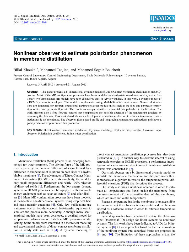
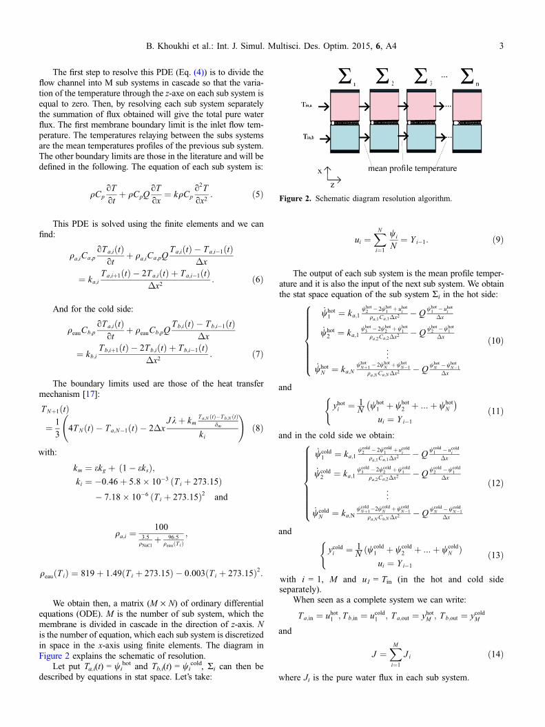
Figures 3 and 4 show the bi dimensional result of temper-ature equation in the flow channels of membrane. As can beseen, the temperature in the hot side decrease along thex and z-axis of membrane, in the same way the cold side tem-perature increase along the x and the z-axis, this phenomenonis called polarization.

A case study from literature has been investigated. Thedata used in our simulations like geometry, physical propertiesand operating conditions are the same used in [4]. Simulationshave been conducted for different inlets temperature. Com-pared with the stationary experimental data in [4].

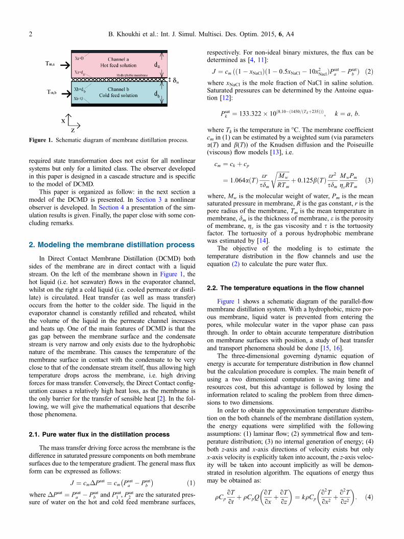
As shown in Figure 5, the computed mass flux densities arein good agreement with the measurements.

3. Nonlinear observer

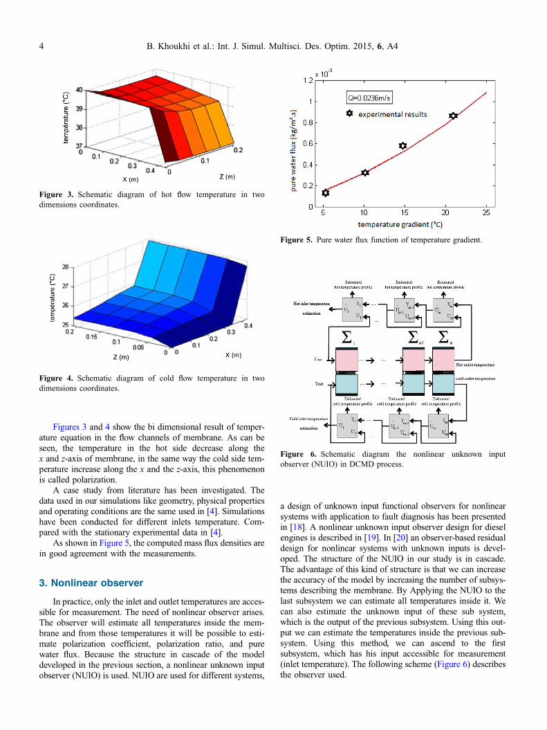
In practice, only the inlet and outlet temperatures are acces-sible for measurement. The need of nonlinear observer arises.The observer will estimate all temperatures inside the mem-brane and from those temperatures it will be possible to esti-mate polarization coefficient, polarization ratio, and purewater flux. Because the structure in cascade of the modeldeveloped in the previous section, a nonlinear unknown inputobserver (NUIO) is used. NUIO are used for different systems,

a design of unknown input functional observers for nonlinearsystems with application to fault diagnosis has been presentedin [18]. A nonlinear unknown input observer design for dieselengines is described in [19]. In [20] an observer-based residualdesign for nonlinear systems with unknown inputs is devel-oped. The structure of the NUIO in our study is in cascade.The advantage of this kind of structure is that we can increasethe accuracy of the model by increasing the number of subsys-tems describing the membrane. By Applying the NUIO to thelast subsystem we can estimate all temperatures inside it. Wecan also estimate the unknown input of these sub system,which is the output of the previous subsystem. Using this out-put we can estimate the temperatures inside the previous sub-system. Using this method, we can ascend to the firstsubsystem, which has his input accessible for measurement(inlet temperature). The following scheme (Figure 6) describesthe observer used.

Figure 3. Schematic diagram of hot flow temperature in twodimensions coordinates.

Figure 4. Schematic diagram of cold flow temperature in twodimensions coordinates.

Figure 5. Pure water flux function of temperature gradient.

Figure 6. Schematic diagram the nonlinear unknown inputobserver (NUIO) in DCMD process.

4 B. Khoukhi et al.: Int. J. Simul. Multisci. Des. Optim. 2015, 6, A4

This structure has a lot of advantages; it is possible toincrease the accuracy of the model by increasing the numberof subsystems. Also, when estimating all temperatures insidethe membrane, we will be able to calculate the estimated fluxin each part of the membrane, calculate the total flux, and then,calculate different parameters such as polarization ratio andpolarization coefficient.

3.1. Development

The NUIO is an observer based on a model, the structureof the hot side observer of the subsystem i is:

_whot1 ¼ ka;1

whot2 � 2whot

1 þ uhoti

qa;1 Ca;1�x2 � Qwhot

1 � uhoti

�x þ L1 Y hoti � Y hot

i

� �

_whot2 ¼ ka;1

whot3 � 2whot

2 þ 1whot1

qa;2 Ca;2�x2 � Qwhot

2 � whot1

�x þ L2 Y hoti � Y hot

i

� �

..

.

_whotN ¼ ka;N

whotNþ1 � 2whot

N þ whotN�1

qa;N Ca;N �x2 � Qwhot

N � whotN�1

�x þ LN Y hoti � Y hot

i

� �

_yhoti ¼ 1

N whot1 þ whot

2 þ � � � þ whotN

� �

uhoti ¼ ayhot

i þ b yhoti � yhot

i

� �

8>>>>>>>>>>>>>>><

>>>>>>>>>>>>>>>:

ð15Þand yi is the outlet temperature, which is accessible for mea-surement. Because of the structure of the model in cascade,the estimated unknown input is the output of the previoussubsystem ui ¼ yði�1Þ this output can be used to estimateall parameters of the previous subsystem (i � 1) and bycontinuing with same principal to the first subsystem wecan estimate all the parameters of the membrane. The samedevelopment is applied to the cold side:

_wcold1 ¼ ka;1

wcold2 � 2wcold

1 þ 1ucoldi

qa;1 Ca;1�x2 � Qwcold

1 � ucoldi

�x þ L1 Y coldi � Y cold

i

� �

_whot2 ¼ kb;2

wcold3 � 2wcold

2 þ 1wcold1

qb;2 Cb;2�x2 � Qwcold

2 � wcold1

�x þ L2 Y coldi � Y cold

i

� �

..

.

_wcoldN ¼ kb;N

wcoldNþ1 � 2wcold

N þ 1wcoldN�1

qb;N Cb;N �x2 � Qwcold

N � wcoldN�1

�x þ LN Y coldi � Y cold

i

� �

_ycoldi ¼ 1

N wcold1 þ wcold

2 þ � � � þ wcoldN

� �

_ucoldi ¼ a _ycold

i þ b ycoldi � _y

cold

i

� �

:

8>>>>>>>>>>>>>>><

>>>>>>>>>>>>>>>:

ð16Þ

4. Simulations results

4.1. Estimation of the pure water flux

The pure water flux is accessible for measurement; it is agood parameter to evaluate the accuracy of the observer byplotting the estimation error between the measured flow andthe estimated flow given by the NUIO. The estimated pure

water flux is given by the following equation (17):

J ¼ cm 1� xNaClð Þ 1� 0:5xNaCl � 10x2Nacl

� �P sat

a � P satb

� �

ð17Þwith

P satk ¼ 133:322 � 10 8:10765� 1450:286= T kþ235ð Þð Þð Þ; k ¼ a; b:

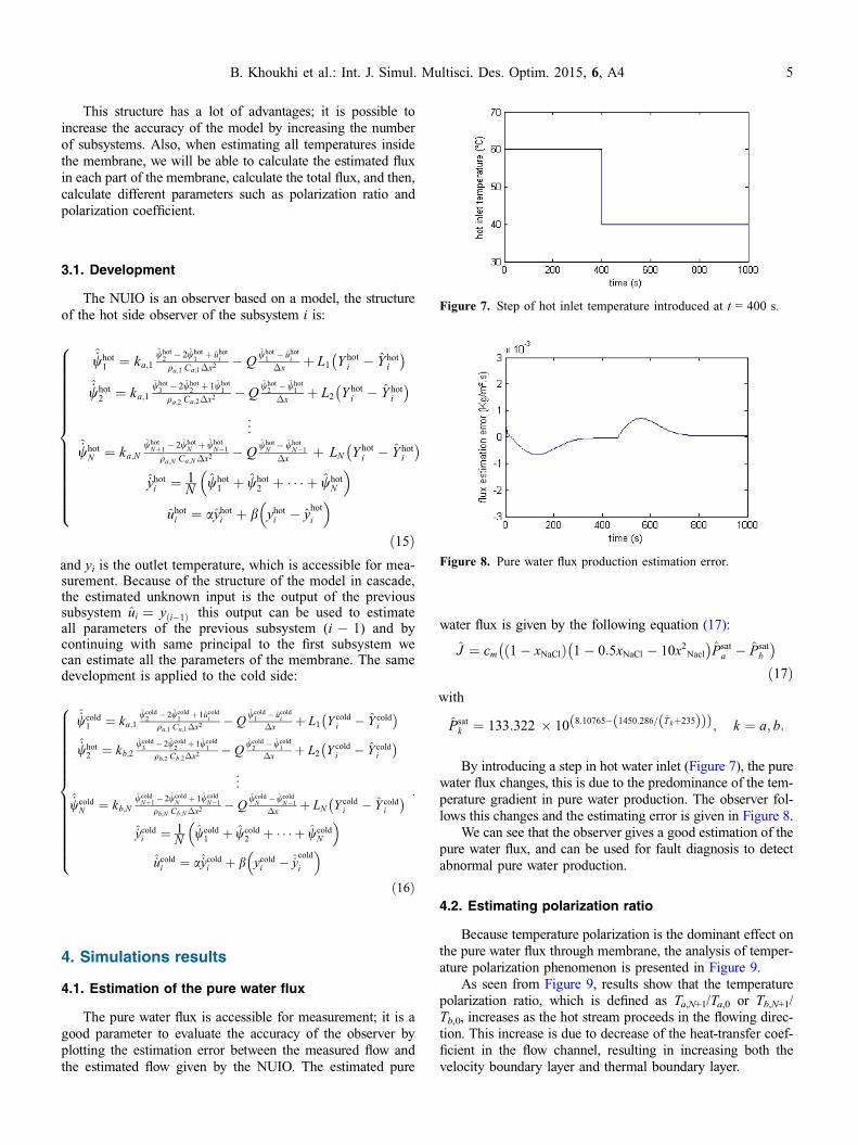
By introducing a step in hot water inlet (Figure 7), the purewater flux changes, this is due to the predominance of the tem-perature gradient in pure water production. The observer fol-lows this changes and the estimating error is given in Figure 8.

We can see that the observer gives a good estimation of thepure water flux, and can be used for fault diagnosis to detectabnormal pure water production.

4.2. Estimating polarization ratio

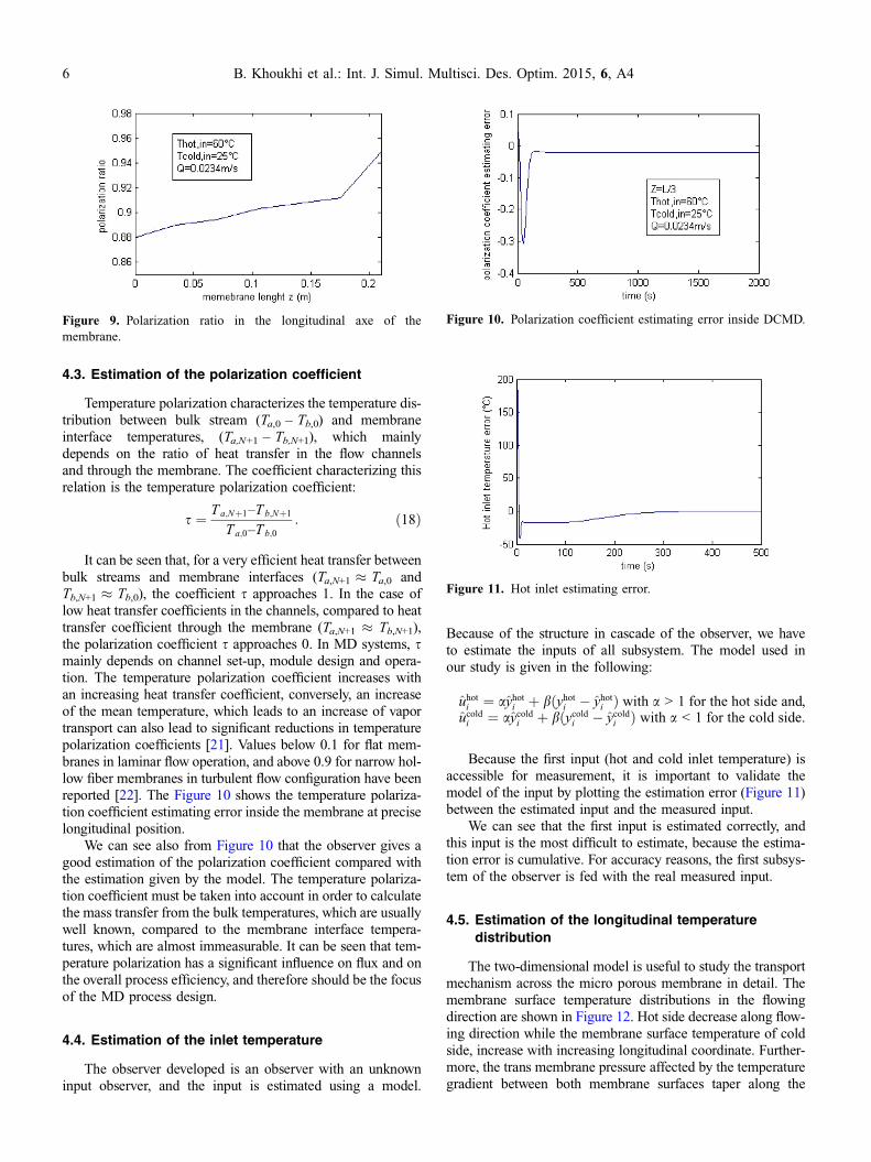
Because temperature polarization is the dominant effect onthe pure water flux through membrane, the analysis of temper-ature polarization phenomenon is presented in Figure 9.

As seen from Figure 9, results show that the temperaturepolarization ratio, which is defined as Ta,N+1/Ta,0 or Tb,N+1/Tb,0, increases as the hot stream proceeds in the flowing direc-tion. This increase is due to decrease of the heat-transfer coef-ficient in the flow channel, resulting in increasing both thevelocity boundary layer and thermal boundary layer.

Figure 7. Step of hot inlet temperature introduced at t = 400 s.

Figure 8. Pure water flux production estimation error.

B. Khoukhi et al.: Int. J. Simul. Multisci. Des. Optim. 2015, 6, A4 5

4.3. Estimation of the polarization coefficient

Temperature polarization characterizes the temperature dis-tribution between bulk stream (Ta,0 – Tb,0) and membraneinterface temperatures, (Ta,N+1 – Tb,N+1), which mainlydepends on the ratio of heat transfer in the flow channelsand through the membrane. The coefficient characterizing thisrelation is the temperature polarization coefficient:

s ¼ T a;Nþ1–T b;Nþ1

T a;0–T b;0: ð18Þ

It can be seen that, for a very efficient heat transfer betweenbulk streams and membrane interfaces (Ta,N+1 � Ta,0 andTb,N+1 � Tb,0), the coefficient s approaches 1. In the case oflow heat transfer coefficients in the channels, compared to heattransfer coefficient through the membrane (Ta,N+1 � Tb,N+1),the polarization coefficient s approaches 0. In MD systems, smainly depends on channel set-up, module design and opera-tion. The temperature polarization coefficient increases withan increasing heat transfer coefficient, conversely, an increaseof the mean temperature, which leads to an increase of vaportransport can also lead to significant reductions in temperaturepolarization coefficients [21]. Values below 0.1 for flat mem-branes in laminar flow operation, and above 0.9 for narrow hol-low fiber membranes in turbulent flow configuration have beenreported [22]. The Figure 10 shows the temperature polariza-tion coefficient estimating error inside the membrane at preciselongitudinal position.

We can see also from Figure 10 that the observer gives agood estimation of the polarization coefficient compared withthe estimation given by the model. The temperature polariza-tion coefficient must be taken into account in order to calculatethe mass transfer from the bulk temperatures, which are usuallywell known, compared to the membrane interface tempera-tures, which are almost immeasurable. It can be seen that tem-perature polarization has a significant influence on flux and onthe overall process efficiency, and therefore should be the focusof the MD process design.

4.4. Estimation of the inlet temperature

The observer developed is an observer with an unknowninput observer, and the input is estimated using a model.

Because of the structure in cascade of the observer, we haveto estimate the inputs of all subsystem. The model used inour study is given in the following:

uhoti ¼ ayhot

i þ bðyhoti � yhot

i Þ with a > 1 for the hot side and,ucold

i ¼ aycoldi þ bðycold

i � ycoldi Þ with a < 1 for the cold side.

Because the first input (hot and cold inlet temperature) isaccessible for measurement, it is important to validate themodel of the input by plotting the estimation error (Figure 11)between the estimated input and the measured input.

We can see that the first input is estimated correctly, andthis input is the most difficult to estimate, because the estima-tion error is cumulative. For accuracy reasons, the first subsys-tem of the observer is fed with the real measured input.

4.5. Estimation of the longitudinal temperaturedistribution

The two-dimensional model is useful to study the transportmechanism across the micro porous membrane in detail. Themembrane surface temperature distributions in the flowingdirection are shown in Figure 12. Hot side decrease along flow-ing direction while the membrane surface temperature of coldside, increase with increasing longitudinal coordinate. Further-more, the trans membrane pressure affected by the temperaturegradient between both membrane surfaces taper along the

Figure 10. Polarization coefficient estimating error inside DCMD.

Figure 11. Hot inlet estimating error.

Figure 9. Polarization ratio in the longitudinal axe of themembrane.

6 B. Khoukhi et al.: Int. J. Simul. Multisci. Des. Optim. 2015, 6, A4

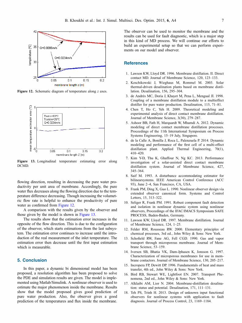
flowing direction, resulting in decreasing the pure water pro-ductivity per unit area of membrane. Accordingly, the purewater flux decreases along the flowing direction due to the tem-perature difference decreasing. Though increasing the volumet-ric flow rate is helpful to enhance the productivity of purewater as confirmed from Figure 12.

A comparison with the results given by the observer andthose given by the model is shown in Figure 13.

The results show that the estimation error increases in theopposite of the flow direction. This is due to the configurationof the observer, which starts estimations from the last subsys-tem. The estimation error continues to increase until the intro-duction of the real measurement of the inlet temperature. Theestimation error then decrease until the first input estimationwhich is measurable.

5. Conclusion

In this paper, a dynamic bi dimensional model has beenproposed, a resolution algorithm has been proposed to solvethe PDE and simulation results are given. The model is imple-mented using Matlab/Simulink. A nonlinear observer is used toestimate the major phenomenon inside the membrane. Resultsshow that the model proposed gives good prediction ofpure water production. Also, the observer gives a goodprediction of the temperatures and flux inside the membrane.

The observer can be used to monitor the membrane and theresults can be used for fault diagnostic, which is a major stepin this kind of MD process. We will continue our efforts tobuild an experimental setup so that we can perform experi-ments on our model and observer.

References

1. Lawson KW, Lloyd DR. 1996. Membrane distillation. II. Directcontact MD. Journal of Membrane Science, 120, 123–133.

2. Koschikowski J, Wieghaus M, Rommel M. 2003. Solarthermal-driven desalination plants based on membrane distil-lation. Desalination, 156, 295–304.

3. de Andrés MC, Doria J, Khayet M, Pena L, Mengual JI. 1998.Coupling of a membrane distillation module to a multieffectdistiller for pure water production. Desalination, 115, 71–81.

4. Chen T, Ho C, Yeh H. 2009. Theoretical modeling andexperimental analysis of direct contact membrane distillation.Journal of Membrane Science, 3(30), 279–287.

5. Ashoor BB, Fath H, Marquardt W, Mhamdi A. 2012. Dynamicmodeling of direct contact membrane distillation processes.Proceedings of the 11th International Symposium on ProcessSystems Engineering, 15–19 July, Singapore.

6. de la Calle A, Bonilla J, Roca L, Palenzuela P. 2014. Dynamicmodeling and performance of the first cell of a multi-effectdistillation plant. Applied Thermal Engineering, 70(1),410–420.

7. Kim Y-D, Thu K, Ghaffour N, Ng KC. 2013. Performanceinvestigation of a solar-assisted direct contact membranedistillation system. Journal of Membrane Science, 427,345–364.

8. Saif M. 1993. A disturbance accommodating estimator forbilinearsystems. IEEE American Control Conference (ACC93), June 2–4, San Francisco, CA, USA.

9. Frank PM, Ding X, Guo L. 1990. Nonlinear observer design viaextended observer canonical form. Systems and ControlLetters, 15, 313–322.

10. Seliger R, Frank PM. 1991. Robust component fault detectionand isolation in nonlinear dynamic system using nonlinearobservers, Proceedings of the IFAC/IMACS Symposium SAFEPROCESS, Baden-Baden, Germany.

11. Lawson KW, Lloyd DR. 1997. Membrane distillation. Journalof Membrane Science, 124, 1–25.

12. Felder RM, Rousseau RW. 2000. Elementary principles ofchemical processes, 3rd ed., John Wiley & Sons: New York.

13. Schofield RW, Fane AG, Fell CGD. 1990. Gas and vaportransport through microporous membrane. Journal of Mem-brane Science, 53–159.

14. Iversen SB, Bhatia VK, Dam-Jphasen K, Jonsson G. 1997.Characterization of microporous membranes for use in mem-brane contactors. Journal of Membrane Science, 130, 205–217.

15. Incropera FP, Dewitt DP. 1996. Fundamentals of heat and masstransfer, 4th ed., John Wiley & Sons: New York.

16. Bird RB, Stewart WE, Lightfoot EN. 2007. Transport Phe-nomena, 2nd ed., John Wiley & Sons: New York.

17. Alklaibi AM, Lior N. 2004. Membrane-distillation desalina-tion: status and potential. Desalination, 171, 111–131.

18. Teh PS, Trinh H. 2013. Design of unknown input functionalobservers for nonlinear systems with application to faultdiagnosis. Journal of Process Control, 23, 1169–1184.

Figure 12. Schematic diagram of temperature along z axes.

Figure 13. Longitudinal temperature estimating error alongDCMD.

B. Khoukhi et al.: Int. J. Simul. Multisci. Des. Optim. 2015, 6, A4 7

19. Boulkroune B, Djemili I, Aitouche A, Cocquempot V. 2013.Nonlinear unknown input observer design for diesel engines.American Control Conference (ACC), June 17–19,Washington, DC, USA, pp. 1076–1081.

20. Teh PS. 2011. Observer-based residual design for nonlinearsystems with unknown inputs. Australian Control Conference,10–11 November, Melbourne, Australia, 198–204.

21. Sherwood TK, Pigford RL, Wilke CR. 1975. Mass transfer,New York, McGraw-Hill.

22. Schofield RW, Fane AG, Fell CJD. 1987. Heat and mass transferin membrane distillation, Journal of Membrane Science, 33,299–313.

Cite this article as: Khoukhi B, Tadjine M & Boucherit MS: Nonlinear observer to estimate polarization phenomenon in membranedistillation. Int. J. Simul. Multisci. Des. Optim., 2015, 6, A4.

8 B. Khoukhi et al.: Int. J. Simul. Multisci. Des. Optim. 2015, 6, A4