統計計算與模擬

政治大學統計系余清祥2004年 3月 29日至 4月 14日第七、九週：矩陣運算http://csyue.nccu.edu.tw

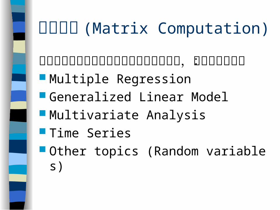
矩陣運算 (Matrix Computation)

矩陣運算在統計分析上扮演非常重要的角色，包括以下方法：

Multiple Regression Generalized Linear Model Multivariate Analysis Time Series Other topics (Random variables)

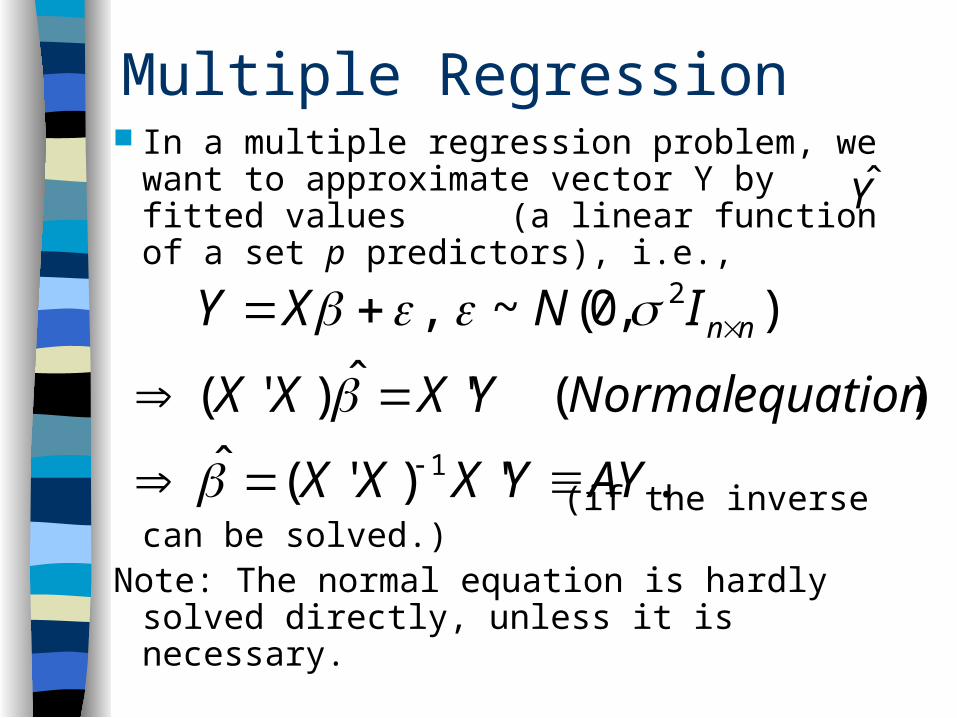
Multiple Regression In a multiple regression problem, we want

to approximate vector Y by fitted values (a linear function of a set p predictors), i.e.,

(if the inverse can be solved.)Note: The normal equation is hardly solved

directly, unless it is necessary.

Y

.')'(ˆ

)('ˆ)'(

),0(~,

1

2

AYYXXX

equationNormalYXXX

INXY nn

In other words, we need to be familiar with matrix computation, such as matrix product and matrix inverse, i.e., X’Y and

If the left hand side matrix is a upper (or lower) triangular matrix, then the estimate can be solved easily,

.)'( 1XX

n

n

p

p

pn

npnp

n

n

YX

YX

YX

YX

a

aa

aaa

aaaa

)'(

)'(

)'(

)'(

ˆ

ˆ

ˆ

ˆ

000

00

0

1

2

1

1

2

1

1,1,1

22322

1131211

1)'( XX

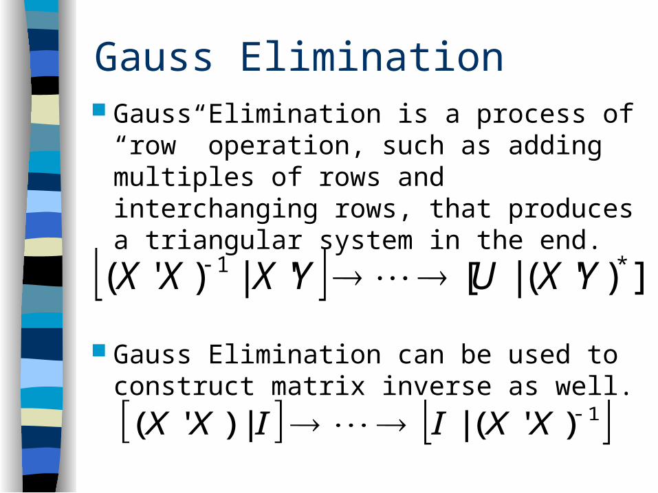
Gauss Elimination Gauss Elimination is a process of “row”

operation, such as adding multiples of rows and interchanging rows, that produces a triangular system in the end.

Gauss Elimination can be used to construct matrix inverse as well.

1)'(||)'( XXIIXX

])'(|['|)'( *1 YXUYXXX

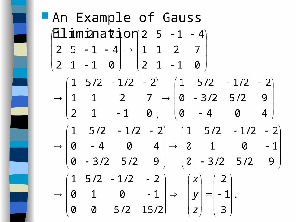
An Example of Gauss Elimination:

.

3

1

2

2/152/500

1010

22/12/51

92/52/30

1010

22/12/51

92/52/30

4040

22/12/51

4040

92/52/30

22/12/51

0112

7211

22/12/51

0112

7211

4152

0112

4152

7211

z

y

x

The idea of Gauss elimination is fine, but it would require a lot of computations.

For example, let X be an n p matrix. Then we need to compute X’X first and then find the upper triangular matrix for (X’X). This requires a number of n2 p multiplications for (X’X) and about another p p(p-1)/2 O(p3) multiplications for the upper triangular matrix.

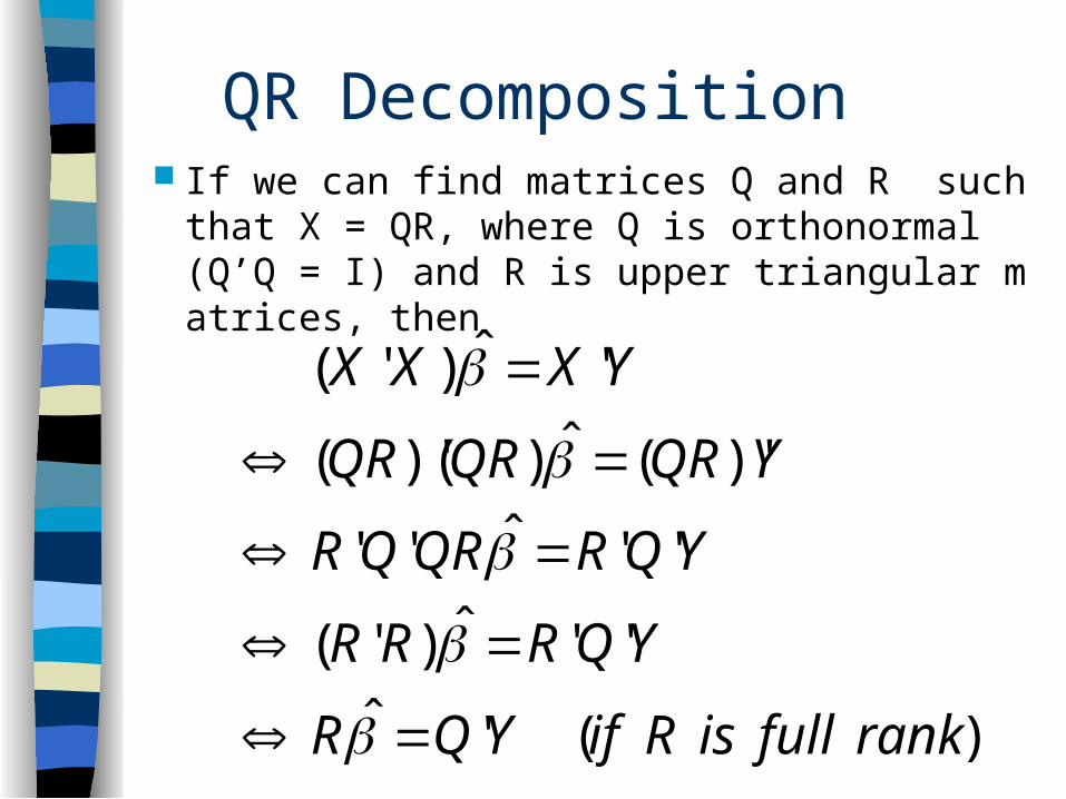
QR Decomposition If we can find matrices Q and R such that

X = QR, where Q is orthonormal (Q’Q = I) and R is upper triangular matrices, then

)('ˆ

''ˆ)'(

''ˆ''

)'(ˆ)()'(

'ˆ)'(

rankfullisRifYQR

YQRRR

YQRQRQR

YQRQRQR

YXXX

Gram-Schmidt Algorithm Gram-Schmidt algorithm is a famous algorith

m for doing QR decomposition. Algorithm: (Q is n p and R is p p.)

for (j in 1:p) {

r[j,j] sqrt(sum(x[,j]^2))

x[,j] x[,j]/r[j,j]

if (j < p) for (k in (j+1):p) {

r[j,k] sum(x[,j]*x[,k])

x[,k] x[,k] – x[,j]*r[j,k]

}

}

Note: Check the function “qr” in S-Plus.

Notes:

(1) Since R is upper triangular, i.e., is easy to obtain,

(2) The idea of the preceding algorithm is

1R

.')'('')'(ˆ

'ˆ

111 yXRRyQRRR

yQR

.'''' RRQRQRXX

QRX

Notes: (continued)

(3) If X is not of full rank, one of the columns will be very close to 0. Thus, and so there will be a divide-by-zero error.

(4) If we apply Gram-Schmidt algorithm to the augmented matrix , the last column will become the residuals of

0jjr

):( yX

.ˆˆ yy

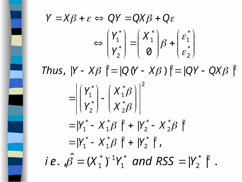
*2

*1

*1

*2

*1

0

X

Y

Y

QQXQYXY

,||||

||||

|||)(|||,

2*2

2*1

*1

2*2

*2

2*1

*1

2

*2

*1

*2

*1

222

YXY

XYXY

X

X

Y

Y

QXQYXYQXYThus

.||)(ˆ.,. 2*2

*1

1*1 YRSSandYXei

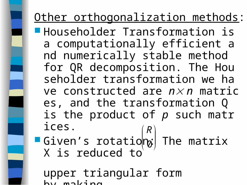
Other orthogonalization methods: Householder Transformation is a computati

onally efficient and numerically stable method for QR decomposition. The Householder transformation we have constructed are n n matrices, and the transformation Q is the product of p such matrices.

Given’s rotation: The matrix X is reduced to

upper triangular form by making

exactly subdiagonal element equal to zero at each step.

0

R

Cholesky Decomposition If A is positive semi-definite, there exists an

upper triangular matrix D such that

since drc = 0 for r > c.

,' ADD

,

.,.

1

11

1

jiii

i

kjkik

i

kjkikij

p

kjkikij

dddddda

soandddaei

Thus, the elements of D equal to

Note: If A is “positive semi-definite” if for all vectors v Rp, we have v’Av 0, where A is a p p matrix. If v’Av = 0 if and only if v = 0, then A is “positive definite.”

./)(

;)(

1

1

1

1

2/1

ii

i

kjkikjiji

i

kjkikiiii

dddad

ddad

Applications of Cholesky decomposition: Simulation of correlated random variables (a

nd also multivariate distributions). Regression

Determinant of a symmetric matrix,

.ˆˆ

ˆ''

'ˆ''ˆ'

forDbacksolveand

DforyXDsolve

yXDDyXXX

DDA '

i

iidDDDA 22)det()'det()det(

Sweep Operator

The normal equation is not solved directly in the preceding methods. But sometimes we need to compute sums of squares and cross-products (SSCP) matrix.

This is particularly useful in stepwise regression, since we need to compute the residual sum of squares (RSS) before and after a certain variable is added or removed.

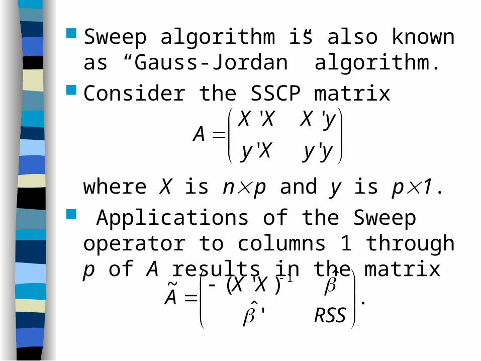
Sweep algorithm is also known as “Gauss-Jordan” algorithm.

Consider the SSCP matrix

where X is n p and y is p1. Applications of the Sweep operator to

columns 1 through p of A results in the matrix

yyXy

yXXXA

''

''

.'ˆ

ˆ)'(~ 1

RSS

XXA

1)'(ˆ'' XXIIyXXX pp

'ˆ)('00'' yPIyyyXy X

Details of Sweep algorithm Step 1: Row 1

Step 2: Row 2

Row 2 minus Row 1 times Xy'

))'(( 1XXtimes

Notes:

(1) If you apply the Sweep operator to columns i1, i2, …, ik, you’ll receive the results from regressing y on

— the corresponding elements in the last column will be the estimated regression coefficients, the (p+1, p+1) element will contain RSS, and so forth.

kiii XXX ,,,21

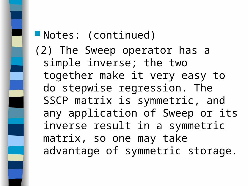
Notes: (continued)

(2) The Sweep operator has a simple inverse; the two together make it very easy to do stepwise regression. The SSCP matrix is symmetric, and any application of Sweep or its inverse result in a symmetric matrix, so one may take advantage of symmetric storage.

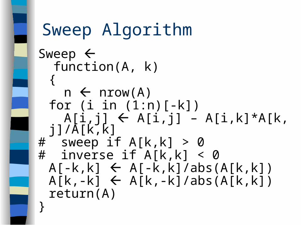
Sweep AlgorithmSweep function(A, k)

{ n nrow(A)

for (i in (1:n)[-k]) A[i,j] A[i,j] – A[i,k]*A[k,j]/A[k,k]

# sweep if A[k,k] > 0# inverse if A[k,k] < 0

A[-k,k] A[-k,k]/abs(A[k,k])A[k,-k] A[k,-k]/abs(A[k,k])

return(A) }

General Least Square (GLM) Consider the model

where with V unknown. Consider the Cholesky decomposition of V,

V = D’D, and let

let

Then y* = X* + with and we may proceed with before.

A special case (WLS): V = diag{v1,…,vn}.

, Xy

),0(~ 2VN

)'.()'(' 11 DDS.'*,'*,'* SandXSXySy

),,0(~ 2VN

Singular Value Decomposition In regression problem, we have

or equivalently,

''' UXUYUXY

*

**1

**1*

0

'0

0

D

VVX

XY

)&'( *1 DVXV

The two orthogonal matrices U and V are associated with the following result:

The Singular-Value Decomposition

Let X be an arbitrary n p matrix with n p. Then there exists orthogonal matrices U: n

n and V: p p such that

,0

~'

DDXVU

.0212

1

p

p

dddwith

d

d

d

Dwhere

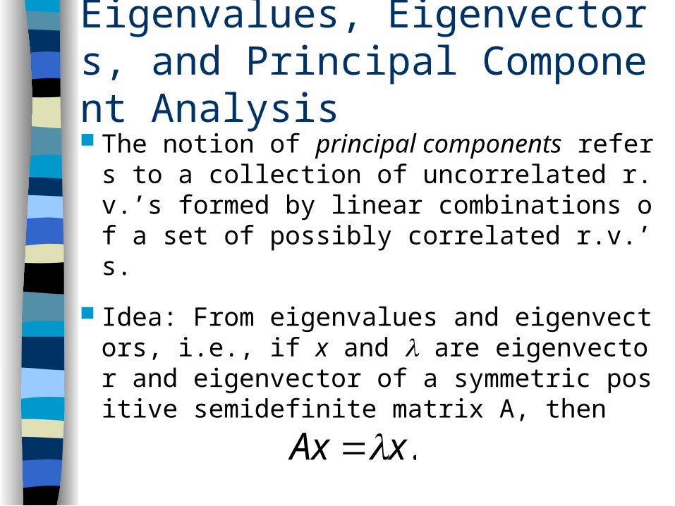
Eigenvalues, Eigenvectors, and Principal Component Analysis The notion of principal components refers to

a collection of uncorrelated r.v.’s formed by linear combinations of a set of possibly correlated r.v.’s.

Idea: From eigenvalues and eigenvectors, i.e., if x and are eigenvector and eigenvector of a symmetric positive semidefinite matrix A, then

.xAx

If A is a symmetric positive semi-definite matrix (p p), then we can find orthogonal matrix such that A = ’, where

Note: This is called the spectral decomposition of A. The ith row of is the eigenvector of A which corresponds to the ith eigenvalue i.

.0, 212

1

p

p

with

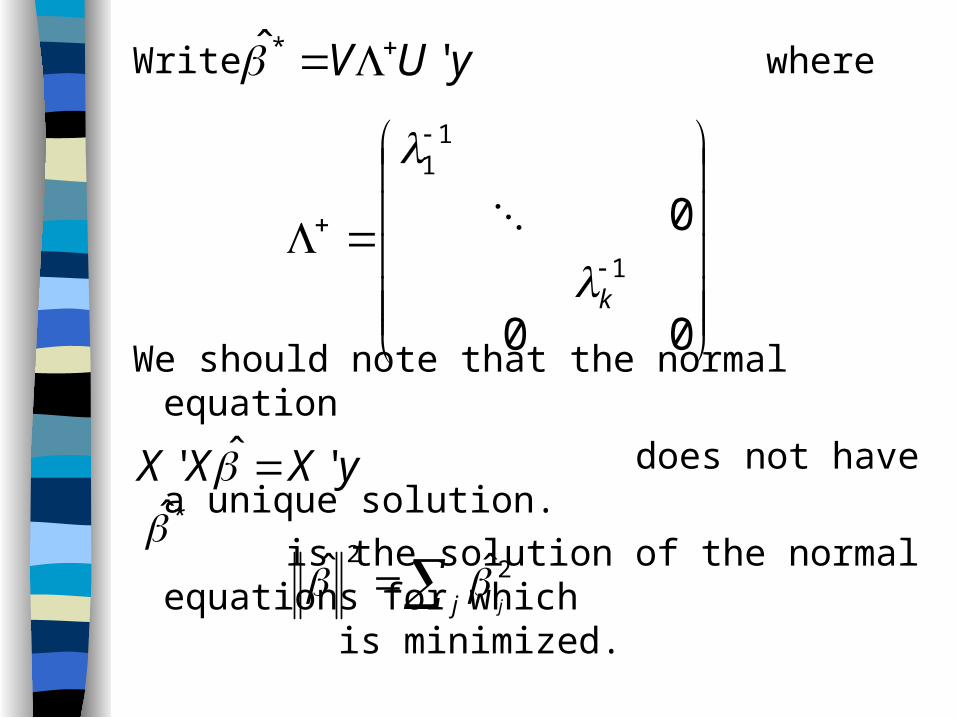
Write where

We should note that the normal equation

does not have a unique solution.

is the solution of the normal equations for which is minimized.

yUV 'ˆ *

00

01

11

k

yXXX 'ˆ' *

j j

22 ˆˆ

Note: There are some handouts from the references regarding “Matrix Computation”

“Numerical Linear Algebra” from Internet Chapters 3 to 6 in Monohan (2001) Chapter 3 in Thisted (1988)

Students are required to read and understand all these materials, in addition to the powerpoint notes.