working with abaqus cae - jahm.com · 1 1 jahm software, inc. working with abaqus cae this is a...

1

1 JAHM Software, Inc.

Working with Abaqus CAE

This is a brief how-to for creating material data files with the MPDB software (https://www.jahm.com/)

and accessing these material data files within Abaqus CAE.

Step 1: On your hard drive create the directory where the your_materials.mpdb files created in the

MPDB software will be saved for use in Abaqus.

a) Do this in Windows explorer if needed.

Step 2: Create your database using the MPDB software

a) Each property must be written to its own file. There is only one property in a file.

b) Start the MPDB software.

c) Select the material you want to add to the database in the normal way. Check “ABAQUS” for

the output format and click the “Display data” button, Figure 1.

d) The window shown in Figure 2 will pop-up and you can select the temperature increment

for the data to be written. Make sure that the “Print property headers for ABAQUS” is not

checked. This option is only used if you want to paste the data directly into your job.inp file

from a text editor and you are not using CAE to create and edit your materials. Click “OK”.

e) The data will be written to the output window as shown in Figure 3.

f) Click the “Write to file” button (Figure 3) to save the data to a text file, Figure 4.

g) If you are writing “mean CTE” data be sure to make note of the “reference temperature” as

written to the note field of the window. This must be manually entered into CAE later. In

this example it is 19.9 C.

h) Repeat steps c – f for as many materials and properties you need. If you have two materials

and need the elastic modulus, mean CTE and stress-strain curve for each material you

should have six files when you have finished.

Step 3: Importing your data into CAE

a) Open your model in CAE and right-click on the “materials” icon and click “Create…” in the

pop-up menu, Figure 5.

b) A new window will open for you to define your material, Figure 6.

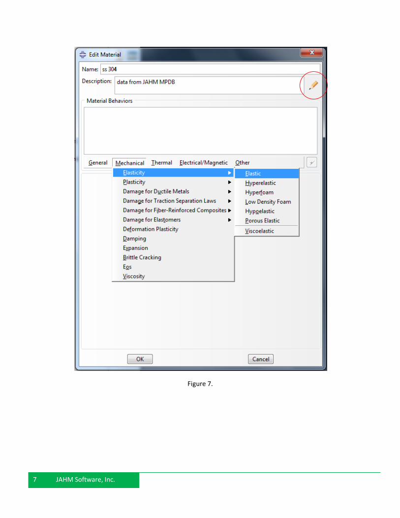
c) Enter the material name and a description (Click the pencil icon to add a comment). Select

the property you want to import data for, Figure 7.

d) Check the “Use temperature-dependent data” option and right-click in the first cell of the

first column and select “Read from file…” from the pop-up menu, Figure 8.

e) A new window will open, click on the file icon (Figure 9) and navigate to the data file created

above in part a in the MPDB software, select it and click “OK”, Figure 10.

f) Click “OK” again in the next window, Figure 11.

2


g) The data will be imported into CAE.

h) Repeat the same steps for the expansion data remembering to enter the reference

temperature, Figure 13.

i) When you import stress-strain data be sure that the “Use temperature-dependent data”

option is checked since the temperature for the curve is also written to the data by MPDB,

Figure 14. This is true even if you only have one temperature or your simulation is not

temperature dependent.

j) If you need to import additional stress-strain data at different temperatures right-click in a

cell in the last data line, then click “Insert after row” in the pop-up menu.

k) Move the cursor to the first cell in the new empty row, Figure 16. Right-click in this cell and

open the data file with the next set of stress-strain data. The additional data will be read-in

and appended, Figure 17.

3


Figure 1.

Figure 2.

4


Figure 3.

5


Figure 4.

Figure 5.

6


Figure 6.

7


Figure 7.

8


Figure 8.

9


Figure 9.

Figure 10.

10


Figure 11.

11


Figure 12.

12


Figure 13.

13


Figure 14.

14


Figure 15.

15


Figure 16.

16


Figure 17.

17


Working with Python

If you use the same materials for several analyses you can create a python script which will define your

materials data in CAE for you. Below is a demo script to define a material called “iron”. Copy this script

into a file called “mats.py” (or any similar name) using a text editor such as Notepad and save it to the

directory where you CAE database file is. In the command part of the CAE window (Figure 18 and 10)

click on the ‘>>>’ button and type:

>>>execfile(‘mats.py’)

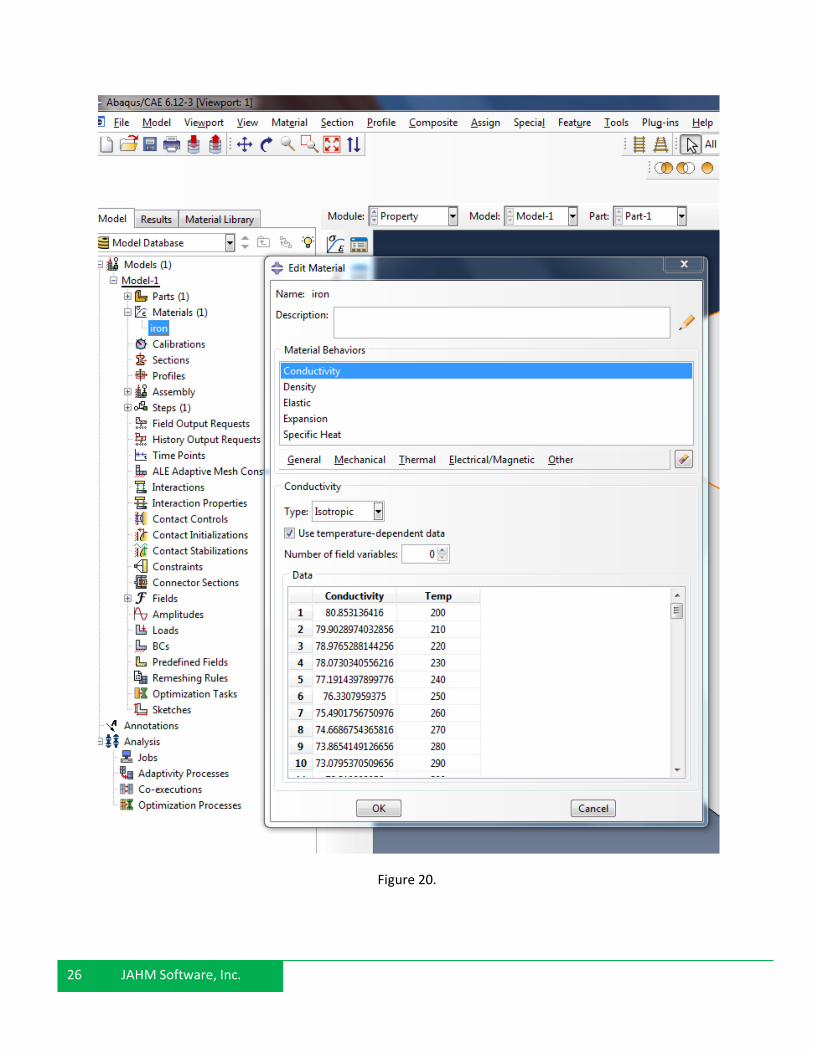
A material named “iron” is created, Figure 20. This script is also available on the web site at:

http://www.jahm.com/pages/python_demo.html for easier copying. You can add as many materials as

you need to the script or write a script file for each material separately.

18


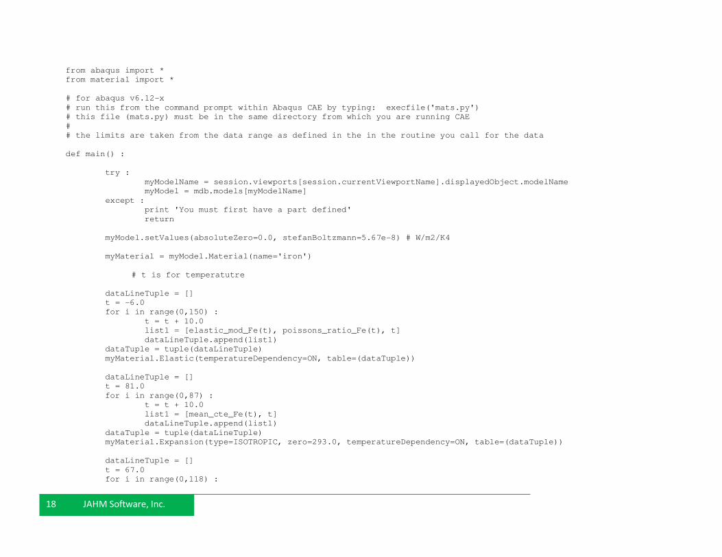
from abaqus import *

from material import *

# for abaqus v6.12-x

# run this from the command prompt within Abaqus CAE by typing: execfile('mats.py')

# this file (mats.py) must be in the same directory from which you are running CAE

#

# the limits are taken from the data range as defined in the in the routine you call for the data

def main() :

try :

myModelName = session.viewports[session.currentViewportName].displayedObject.modelName

myModel = mdb.models[myModelName]

except :

print 'You must first have a part defined'

return

myModel.setValues(absoluteZero=0.0, stefanBoltzmann=5.67e-8) # W/m2/K4

myMaterial = myModel.Material(name='iron')

# t is for temperatutre

dataLineTuple = []

t = -6.0

for i in range(0,150) :

t = t + 10.0

list1 = [elastic_mod_Fe(t), poissons_ratio_Fe(t), t]

dataLineTuple.append(list1)

dataTuple = tuple(dataLineTuple)

myMaterial.Elastic(temperatureDependency=ON, table=(dataTuple))

dataLineTuple = []

t = 81.0


t = t + 10.0

list1 = [mean_cte_Fe(t), t]



myMaterial.Expansion(type=ISOTROPIC, zero=293.0, temperatureDependency=ON, table=(dataTuple))

dataLineTuple = []

t = 67.0


19


t = t + 10.0

list1 = [thermal_cond_Fe_solid(t), t]



myMaterial.Conductivity(type=ISOTROPIC, temperatureDependency=ON, table=(dataTuple))

dataLineTuple = []

t = -1.0


t = t + 10.0

list1 = [specific_heat_Fe_solid(t), t]



myMaterial.SpecificHeat(temperatureDependency=ON, table=(dataTuple))

dataLineTuple = []

t = 81.0


t = t + 10.0

list1 = [density_Fe_solid(t), t]



myMaterial.Density(temperatureDependency=ON, table=(dataTuple))

dataLineTuple = []

# s = strain, t = temperature data was taken at, rate = strain rate data was taken at

s = -0.01

t = 773 # only needed if you want to enter the temperature of the data

rate = 0.01 # only need if you want to enter the strain rate of the test


s = s + 0.01

# list1 = [Iron_sscc_3_4(s), s] # if you do not want to enter the temperature or strain rate use this

# list1 = [Iron_sscc_3_4(s), s, t] # if you do not want to enter the strain rate use this line

list1 = [Iron_sscc_3_4(s), s, rate, t] # if you want to enter the strain rate use this line


s = -0.01




s = s + 0.01




20



s = -0.01




s = s + 0.01





s = -0.01


rate = 0.1 # only need if you want to enter the strain rate of the data


s = s + 0.01






# if you want to enter the stress use this line

# myMaterial.Plastic(table=(dataTuple))

# if you want to enter the stress and temperature use this line

# myMaterial.Plastic(temperatureDependency=ON, table=(dataTuple))

# if you want to enter the stress, strain rate and temperature use this line

myMaterial.Plastic(temperatureDependency=ON, rate=ON, table=(dataTuple))

##################################################################################################

def poissons_ratio_Fe(t) :

# Poissons ratio is unitless

# t must be in degrees Kelvin for these equations

if t >= 4.0 and t <= 273.0 :

return -6.293870E-13*t*t*t*t + 5.370994E-10*t*t*t -6.309382E-08*t*t + 4.180781E-08*t + 2.850633E-01

elif t > 273.0 and t <= 1053.0 :

return 1.246582E-11*t*t*t -3.856929E-08*t*t + 7.030261E-05*t + 2.712267E-01

elif t > 1053.0 and t <= 1500.0 :

return 1.661461E-09*t*t -1.242823E-06*t + 3.165268E-01

elif t < 4.0 :

return 2.850625E-01

elif t > 1500.0 :

return 3.184009E-01

21


##################################################################################################

def elastic_mod_Fe(t) :

# Note: approximate values for plain carbon and low alloy steels;

# values below 273K were calculated from C11, C12, C44

# elastic modulus is in units of Pa


if t >= 4.0 and t <= 273.0 :

return -1.145454*t*t*t*t + 9.266601E+02*t*t*t -3.051404E+05*t*t + 5.020008E+06*t + 2.217366E+11

elif t > 273.0 and t <= 1050.0 :

return -1.063196E+05*t*t + 3.572844E+07*t + 2.109875E+11

elif t > 1050.0 and t <= 1500.0 :

return -6.773810E+07*t + 2.024261E+11

elif t < 4.0 :

return 2.217519E+11

elif t > 1500.0 :

return 1.008190E+11

##################################################################################################

def mean_cte_Fe(t) :

# the reference temperature is 293K; 8% error

# data is in units of 1/K


if t >= 91.0 and t < 410.0 :

return 8.156945e-014*t*t*t -9.244895e-011*t*t +3.775811e-008*t +6.517108e-006

elif t >= 410.0 and t <= 960.0 :

return 4.782671e-017*t*t*t*t -1.357633e-013*t*t*t +1.324312e-010*t*t -4.591434e-008*t +1.664716e-005

elif t < 91.0 :

return 9.248995e-006

elif t > 960.0 :

return 1.512476e-005

##################################################################################################

def thermal_cond_Fe_solid(t) :

# data is in units of W/(m-K)


if t >= 77.0 and t <= 1255.0 :

return 9.690376e-011*t*t*t*t -2.494362e-007*t*t*t +2.508465e-004*t*t -1.697584e-001*t +1.066114e+002

elif t < 77.0 :

return 9.491680e+001

elif t > 1255.0 :

return 3.599398e+001

22


##################################################################################################

def specific_heat_Fe_solid(t) :

# 1.5% to 5% error

# data is in units of J/(kg-K)


if t >= 1.0 and t < 20.0 :

return 8.786827e-006*t*t*t*t +3.434114e-005*t*t*t +3.543513e-003*t*t +7.343790e-002*t +1.640777e-002

elif t >= 20.0 and t < 130.0 :

return 5.251765e-008*t*t*t*t*t -1.807849e-005*t*t*t*t +1.972324e-003*t*t*t -5.588171e-002*t*t

+9.005499e-001*t -4.129967e+000

elif t >= 130.0 and t < 500.0 :

return -1.683141e-008*t*t*t*t +2.868283e-005*t*t*t -1.780930e-002*t*t +5.191206e+000*t -1.438118e+002

elif t >= 500.0 and t < 1000.0 :

return 1.852870e-008*t*t*t*t -4.990048e-005*t*t*t +5.023704e-002*t*t -2.189081e+001*t +3.998510e+003

elif t >= 1000.0 and t < 1042.0 :

return 6.672367e-004*t*t*t -1.889510e+000*t*t +1.783888e+003*t -5.606426e+005

elif t >= 1042.0 and t < 1184.0 :

return 3.231248e-006*t*t*t*t -1.504264e-002*t*t*t +2.625897e+001*t*t -2.037174e+004*t +5.927268e+006

elif t >= 1184.0 and t < 1665.0 :

return 1.496811e-001*t +4.295303e+002

elif t >= 1665.0 and t <= 1809.0 :

return 1.778200e-001*t +4.402844e+002

elif t < 1.0 :

return 9.343231e-002

elif t > 1809.0 :

return 7.619609e+002

##################################################################################################

def density_Fe_solid(t) :

# the reference temperature is 293K; 8% error

# data is in units of g/cm^3


if t >= 91.0 and t < 190.0 :

return -6.010914e-009*t*t*t +2.196832e-006*t*t -4.306436e-004*t +7.924000e+000

elif t >= 190.0 and t <= 960.0 :

return 1.470685e-010*t*t*t -3.511597e-007*t*t -1.002710e-004*t +7.910967e+000

elif t < 91.0 :

return 7.898474e+000

elif t > 960.0 :

return 7.621195e+000

23


##################################################################################################

def Iron_sscc_3_3(s) :

# bal Fe, 0.007 C, 0.03 Mn, 0.005 S, 0.003 P (wt%)

# forged at 1173K and annealed at 1023K for 2 h, alpha iron, tested

# at 773K; measured in compression, strain rate of 0.1/s

# data is in units of Pa

if s >= 0.000000e+000 and s < 5.000000e-002 :

return -1.203463e+012*s*s*s*s +4.772727e+011*s*s*s -6.325758e+010*s*s +3.847403e+009*s +1.363636e+008

elif s >= 5.000000e-002 and s <= 5.500000e-001 :


else :

return 1.000000e+100

##################################################################################################


# bal Fe, 0.007 C, 0.03 Mn, 0.005 S, 0.003 P (wt%)




if s >= 0.000000e+000 and s < 2.500000e-002 :


elif s >= 2.500000e-002 and s <= 5.500000e-001 :

return 4.499607e+009*s*s*s*s*s -7.743565e+009*s*s*s*s +5.084152e+009*s*s*s -1.686610e+009*s*s

+3.486258e+008*s +4.745064e+007

else :

return 1.000000e+100

##################################################################################################


# bal Fe, 0.007 C, 0.03 Mn, 0.005 S, 0.003 P (wt%)




if s >= 0.000000e+000 and s < 2.500000e-002 :

return 3.090909e+011*s*s*s -5.772727e+010*s*s +3.613636e+009*s +9.090909e+007

elif s >= 2.500000e-002 and s <= 5.500000e-001 :

return 2.608081e+009*s*s*s*s*s -7.291472e+009*s*s*s*s +6.866451e+009*s*s*s -3.033937e+009*s*s

+7.530978e+008*s +1.329767e+008

else :

return 1.000000e+100

##################################################################################################

24



# bal Fe, 0.007 C, 0.03 Mn, 0.005 S, 0.003 P (wt%)




if s >= 0.000000e+000 and s < 5.000000e-002 :

return 5.194805e+009*s*s*s -1.688312e+009*s*s +2.012987e+008*s +2.597403e+007

elif s >= 5.000000e-002 and s <= 5.500000e-001 :


else :

return 1.000000e+100

##################################################################################################

# call main to get program started

main()

25


Figure 18.

Figure 19.

26


Figure 20.

working with abaqus cae - jahm.com · 1 1 jahm software, inc. working with abaqus cae this is a...

Documents