trademarks and legal notices - uni-due.deinfo.statik.uni-due.de/lehre/cm/aos/scripts/abaqus/... ·...
TRANSCRIPT


Trademarks and Legal Notices
CAUTIONARY NOTICE TO USERS:
This manual is intended for qualified users who will exercise sound engineering judgment and expertise in the use of the ABAQUS Software. The ABAQUS
Software is inherently complex, and the examples and procedures in this manual are not intended to be exhaustive or to apply to any particular situation.
Users are cautioned to satisfy themselves as to the accuracy and results of their analyses.
ABAQUS, Inc. will not be responsible for the accuracy or usefulness of any analysis performed using the ABAQUS Software or the procedures, examples,
or explanations in this manual. ABAQUS, Inc. shall not be responsible for the consequences of any errors or omissions that may appear in this manual.
ABAQUS, INC. DISCLAIMS ALL EXPRESS OR IMPLIED REPRESENTATIONS ANDWARRANTIES, INCLUDING ANY IMPLIEDWARRANTY
OF MERCHANTABILITY OR FITNESS FOR A PARTICULAR PURPOSE OF THE CONTENTS OF THIS MANUAL.
IN NO EVENT SHALL ABAQUS, INC. OR ITS THIRD-PARTY PROVIDERS BE LIABLE FOR ANY INDIRECT, INCIDENTAL, PUNITIVE,
SPECIAL, OR CONSEQUENTIAL DAMAGES (INCLUDING WITHOUT LIMITATION DAMAGES FOR LOSS OF BUSINESS PROFITS,
BUSINESS INTERRUPTION, OR LOSS OF BUSINESS INFORMATION) EVEN IF ABAQUS, INC. HAS BEEN ADVISED OF THE POSSIBILITY
OF SUCH DAMAGES.
The ABAQUS Software described in this manual is available only under license from ABAQUS, Inc. and may be used or reproduced only in accordance
with the terms of such license.
This manual and the software described in this manual are subject to change without prior notice.
No part of this manual may be reproduced or distributed in any form without prior written permission of ABAQUS, Inc.
©ABAQUS, Inc. 2004. All rights reserved.
Printed in the United States of America.
U.S. GOVERNMENT USERS: The ABAQUS Software and its documentation are “commercial items,” specifically “commercial computer software” and
“commercial computer software documentation,” and consistent with FAR 12.212 and DFARS 227.7202, as applicable, are provided under license to the
U.S. Government, with restricted rights.
TRADEMARKS
The trademarks and service marks (“trademarks) in this manual are the property of ABAQUS, Inc. or third parties. You are not permitted to use these
trademarks without the prior written consent of ABAQUS, Inc. or such third parties.
The following are trademarks or registered trademarks of ABAQUS, Inc. or its subsidiaries in the United States and/or other countries: ABAQUS,
ABAQUS/Standard, ABAQUS/Explicit, ABAQUS/CAE, ABAQUS/Viewer, ABAQUS/Aqua, ABAQUS/Design, ABAQUS/Foundation, and the
ABAQUS Logo.
Other company, product, and service names may be trademarks or service marks of their respective owners. For additional information, see the Trademark
and License Notices in the ABAQUS Version 6.5 Release Notes.

ABAQUS Offices and Representatives
ABAQUS, Inc. ABAQUS Europe BVRising Sun Mills Gaetano Martinolaan 95166 Valley Street P. O. Box 1637Providence, RI 02909-2499 6201 BP MaastrichtTel: +1 401 276 4400 The NetherlandsFax: +1 401 276 4408 Tel: +31 43 356 6906E-mail: [email protected] Fax: +31 43 356 6908http://www.abaqus.com E-mail: [email protected]
Sales, Support, and Services
UNITED STATES
ABAQUS Central, Inc. ABAQUS East, LLC1440 Innovation Place 300 Centerville Road, Suite 209WWest Lafayette, IN 47906-1000 Warwick, RI 02886-0201Tel: +1 765 497 1373 Tel: +1 401 739 3637Fax: +1 765 497 4444 Fax: +1 401 739 3302E-mail: [email protected] E-mail: [email protected]
ABAQUS Erie, Inc. ABAQUS Great Lakes, Inc.3601 Green Road, Suite 316 14500 Sheldon Road, Suite 160Beachwood, OH 44122 Plymouth, MI 48170-2408Tel: +1 216 378 1070 Tel: +1 734 451 0217Fax: +1 216 378 1072 Fax: +1 734 451 0458E-mail: [email protected] E-mail: [email protected]
ABAQUS South, Inc. ABAQUS West, Inc.3700 Forums Drive, Suite 101 39221 Paseo Padre Parkway, Suite FFlower Mound, TX 75028 Fremont, CA 94538-1611Tel: +1 214 513 1600 Tel: +1 510 794 5891Fax: +1 214 513 1700 Fax: +1 510 794 1194E-mail: [email protected] E-mail: [email protected]
ARGENTINA AUSTRALIA
KB Engineering S. R. L. Worley Advanced AnalysisFlorida 274 - Oficina 35 Level 17, 300 Flinders Street1005 Buenos Aires Melbourne, Vic 3000Argentina Tel: +61 3 8612 5132Tel: +54 11 4326 9176/7542 Fax: +61 3 9205 0573Fax: +54 11 4326 2424 E-mail: [email protected]: [email protected]

AUSTRIA BENELUX
ABAQUS Austria GmbH ABAQUS Benelux BVZinckgasse 20-22/2/13 Huizermaatweg 576A-1150 Vienna 1276 LN HuizenAustria The NetherlandsTel: +43 1 929 16 25-0 Tel: +31 35 52 58 424Fax: +43 1 929 16 25-20 Fax: +31 35 52 44 257E-mail: [email protected] E-mail: [email protected]
CHINA CZECH REPUBLIC
ABAQUS China Synerma s. r. o.Room A-2703, Eagle Plaza Huntirov 58No. 26 Xiao Yun Rd. 468 22 SkuhrovBeijing, 100016 Czech RepublicP. R. China Tel: +420 603 145 769Tel: +86 01 84580366 Fax: +420 603 181 944Fax: +86 01 84580360 E-mail: [email protected]: [email protected]
FRANCE GERMANY (Aachen)
ABAQUS France SAS ABAQUS Deutschland GmbH7 rue Jean Mermoz, Bat. A Theaterstraße 30-3278000 Versailles D-52062 AachenTel: +33 01 39 24 15 40 Tel: +49 241 474010Fax: +33 01 39 24 15 45 Fax: +49 241 4090963E-mail: [email protected] E-mail: [email protected]
GERMANY (Munich) INDIA (Chennai)
ABAQUS Deutschland GmbH ABAQUS Engineering India (Pvt.) Ltd.Sendlinger-Tor-Platz 8 3M, Prince ArcadeD-80336 München 22-A Cathedral RoadTel: +49 89 5999 1768 Chennai, 600 086Fax: +49 89 5999 1767 Tel: +91 44 28114624E-mail: [email protected] Fax: +91 44 28115087
E-mail: [email protected]
ITALY JAPAN (Tokyo)
ABAQUS Italia s.r.l. ABAQUS, Inc.Via Domodossola, 17 3rd Floor, Akasaka Nihon Building20145 Milano (MI) 5-24, Akasaka 9-chome, Minato-kuTel: +39 02 39211211 Tokyo, 107-0052Fax: +39 02 31800064 Tel: +81 3 5474 5817E-mail: [email protected] Fax: +81 3 5474 5818
E-mail: [email protected]

JAPAN (Osaka) KOREA
ABAQUS, Inc. ABAQUS Korea, Inc.9th Floor, Higobashi Watanabe Building Suite 306, Sambo Building6-10, Edobori 1-chome, Nishi-ku 13-2 Yoido-Dong, Youngdeungpo-kuOsaka, 550-0002 Seoul, 150-010Tel: +81 6 4803 5020 Tel: +82 2 785 6707Fax: +81 6 4803 5021 Fax: +82 2 785 6709E-mail: [email protected] E-mail: [email protected]
MALAYSIA NEW ZEALAND
Worley Advanced Analysis Matrix Applied Computing Ltd.19th Floor, Empire Tower P. O. Box 56-316, AucklandCity Square Centre Courier: Unit 2-5, 72 Dominion Road, Mt Eden,182 Jalan Tun Razak Auckland50400 Kuala Lumpur Tel: +64 9 623 1223Tel: +60 3 2161 2266 Fax: +64 9 623 1134Fax: +60 3 2161 4266 E-mail: [email protected]: [email protected]
POLAND RUSSIA, BELARUS & UKRAINE
BudSoft Sp. z o.o. TESIS Ltd.61-807 Poznań Office 701-703,Sw. Marcin 58/64 18, Unnatov Str.Tel: +48 61 8508 466 127083 Moscow, RussiaFax: +48 61 8508 467 Tel: +7 095 212-44-22E-mail: [email protected] Fax: +7 095 212-42-62
E-mail: [email protected]
SINGAPORE SOUTH AFRICA
Worley Advanced Analysis Finite Element Analysis Services (Pty) Ltd.491B River Valley Road Unit 4, The Waverley#09-01 Valley Point Wyecroft RoadSingapore, 248373 Mowbray 7700Tel: +65 6735 8444 Tel: +27 21 448 7608Fax: +65 6735 7444 Fax: +27 21 448 7679E-mail: [email protected] E-mail: [email protected]

SPAIN SWEDEN
Principia Ingenieros Consultores, S.A. ABAQUS ScandinaviaVelázquez, 94 FEM-Tech ABE-28006 Madrid Pilgatan 8cTel: +34 91 209 1482 SE-72130 VästeråsFax: +34 91 575 1026 Tel: +46 21 12 64 10E-mail: [email protected] Fax: +46 21 18 12 44
E-mail: [email protected]
TAIWAN THAILAND
APIC Worley Advanced Analysis11F, No. 71, Sung Chiang Road 333 Lao Peng Nguan 1 BuildingTaipei, 10428 20th Floor Unit BTel: +886 02 25083066 Soi ChaypuangFax: +886 02 25077185 Vibhavadi-Rangsit RoadE-mail: [email protected] Ladyao, Jatujak
Bangkok 10900ThailandTel: +66 2 689 3000Fax: +66 2 618 8109E-mail: [email protected]
TURKEY UNITED KINGDOM (Cheshire)
A-Ztech Ltd. ABAQUS UK Ltd.Perdemsac Plaza, Teknoloji Evi The Genesis CentreBayar Cad., Gulbahar Sok., No: 17 Science Park South, BirchwoodKozyatagi Warrington, Cheshire WA3 7BH34742 Istanbul Tel: +44 1 925 810166TURKIYE Fax: +44 1 925 810178Tel: +90 216 361 8850 E-mail: [email protected]: +90 216 361 8851E-mail: [email protected]

Sales Only
UNITED STATES
ABAQUS East, LLC, Mid-Atlantic Office ABAQUS South, Inc., Southeast Office114 Zachary Court 484 Broadstone WayForest Hill, MD 21050 Acworth, GA 30101Tel: +1 410 420 8587 Tel: +1 770 795 0960Fax: +1 410 420 8908 Fax: +1 770 795 7614E-mail: [email protected] E-mail: [email protected]
ABAQUS West, Inc., Southern CA and AZ Office ABAQUS West, Inc., Rocky Mountains Office1100 Irvine Boulevard #248 6910 Cordwood Ct.Tustin, CA 92780 Boulder, CO 80301Tel: +1 714 731 5895 Tel: +1 303 664 5444Fax: +1 714 242 7002 Fax: +1 303 200 9481E-mail: [email protected] E-mail: [email protected]
FINLAND INDIA (Pune)
ABAQUS Finland Oy ABAQUS Engineering Analysis Solutions (Pvt.) Ltd.Tekniikantie 12 C-9, 3rd FloorFIN-02150 Espoo Bramha Estate, Kondwa RoadTel: +358 9 2517 2973 Pune-411040Fax: +358 9 2517 2200 Tel: +91 20 30913739E-mail: [email protected] E-mail: [email protected]
UNITED KINGDOM (Kent)
ABAQUS UK Ltd.Great Hollanden Business Centre, Unit AMill Lane, UnderriverSevenoaks, Kent TN15 OSQTel: +44 1 732 834930Fax: +44 1 732 834720E-mail: [email protected]

Preface
This section lists various resources that are available for help with using ABAQUS, including technical
engineering and systems support, training seminars, and documentation.
Support
ABAQUS, Inc., offers both technical engineering support and systems support for ABAQUS. Technical
engineering and systems support are provided through the nearest local support office. You can contact
our offices by telephone, fax, electronic mail, the ABAQUS web-based support system, or regular mail.
Information on how to contact each office is listed in the front of each ABAQUS manual. The ABAQUS
Online Support System (AOSS) is accessible through the MY ABAQUS section of the ABAQUS Home
Page (www.abaqus.com). When contacting your local support office, please specify whether you would
like technical engineering support (you have encountered problems performing an ABAQUS analysis or
creating a model in ABAQUS) or systems support (ABAQUS will not install correctly, licensing does not
work correctly, or other hardware-related issues have arisen).
The ABAQUS Online Support System has a knowledge database of ABAQUS Answers. The ABAQUS
Answers are solutions to questions that we have had to answer or guidelines on how to use ABAQUS. We
welcome any suggestions for improvements to the support program or documentation. We will ensure that
any enhancement requests you make are considered for future releases. If you wish to file a complaint about
the service or products provided by ABAQUS, refer to the ABAQUS Home Page.
Technical engineering support
ABAQUS technical support engineers can assist in clarifyingABAQUS features and checking errors by giving
both general information on using ABAQUS and information on its application to specific analyses. If you
have concerns about an analysis, we suggest that you contact us at an early stage, since it is usually easier to
solve problems at the beginning of a project rather than trying to correct an analysis at the end.
Please have the following information ready before calling the technical engineering support hotline, and
include it in any written contacts:
• Your site identifier, which can be obtained by typing abaqus whereami at your system prompt (or by
selecting Help→On Version from the main menu bar in ABAQUS/CAE or ABAQUS/Viewer).
• The version of ABAQUS that are you using.
– The version numbers for ABAQUS/Standard and ABAQUS/Explicit are given at the top of the data
(.dat) file.
– The version numbers for ABAQUS/CAE and ABAQUS/Viewer can be found by selecting
Help→On Version from the main menu bar.
– The version numbers for the ABAQUS Interface for MOLDFLOW and the ABAQUS Interface for
MSC.ADAMS are output to the screen.
– The version number for ABAQUS for CATIA V5 can be found by selecting Help→About
ABAQUS for CATIA V5 from the main menu bar in either of the ABAQUS for CATIA V5
workbenches.
i

• The type of computer on which you are running ABAQUS.
• The symptoms of any problems, including the exact error messages, if any.
• Workarounds or tests that you have already tried.
When calling for support about a specific problem, any available ABAQUS output files may be helpful in
answering questions that the support engineer may ask you.
The support engineer will try to diagnose your problem from the model description and a description of
the difficulties you are having. The support engineer may need model sketches, which can be sent via fax,
e-mail, or regular mail. Plots of the final results or the results near the point that the analysis terminated may
also be needed to understand what may have caused the problem.
If the support engineer cannot diagnose your problem from this information, you may be asked to
supply the input data. The data can be attached to a support incident in the ABAQUS Online Support
System. It may also be sent by means of e-mail, tape, disk, or ftp. Please check the ABAQUS Home Page
(http://www.abaqus.com) for the media formats that are currently accepted.
All support incidents are tracked in the ABAQUS Online Support System. This enables you (as well as
the support engineer) to monitor the progress of a particular problem and to check that we are resolving support
issues efficiently. To use the ABAQUS Online Support System, you need to register with the system. Visit the
MY ABAQUS section of the ABAQUS Home Page for instructions on how to register. If you are contacting
us by means outside the AOSS to discuss an existing support problem and you know the incident number,
please mention it so that we can consult the database to see what the latest action has been and, thus, give
you more efficient support as well as avoid duplication of effort. In addition, please give the receptionist the
support engineer’s name if contacting us via telephone or include it at the top of any e-mail correspondence.
Systems support
ABAQUS systems support engineers can help you resolve issues related to the installation and running of
ABAQUS, including licensing difficulties, that are not covered by technical engineering support.
You should install ABAQUS by carefully following the instructions in the ABAQUS Installation and
Licensing Guide. If you are able to complete the installation, please make sure that the product verification
procedure was run successfully at the end of the installation procedure. Successful verification for licensed
products would indicate that you can run these products on your computer; unsuccessful verification for
licensed products indicates problems with the installation or licensing (or both). If you encounter problems
with the installation, licensing, or verification, first review the instructions in the ABAQUS Installation and
Licensing Guide to ensure that they have been followed correctly. If this does not resolve the problems,
consult the ABAQUSAnswers database in the ABAQUSOnline Support System for information about known
installation problems. If this does not address your situation, please create an incident in the AOSS and
describe your problem, including the output from abaqus info=support. If you call, mail, e-mail, or fax
us about a problem (instead of using the AOSS), please provide the output from abaqus info=support. It
is important that you provide as much information as possible about your problem: error messages from an
aborted analysis, output from the abaqus info=support command, etc.
ii

ABAQUS Web server
For users connected to the Internet, many questions can be answered by visiting the ABAQUS Home Page
on the World Wide Web at
http://www.abaqus.com
The information available on the ABAQUS Home Page includes:
• Link to the AOSS
• ABAQUS systems information and computer requirements
• ABAQUS performance data
• Error status reports
• ABAQUS documentation price list
• Training seminar schedule
• ABAQUS Insights newsletter
• Technology briefs
Anonymous ftp site
For users connected to the Internet, ABAQUS maintains useful documents on an anonymous ftp account on
the computer ftp.abaqus.com. Simply ftp to ftp.abaqus.com. Login as user anonymous, and type your e-mail
address as your password. Directions will come up automatically upon login.
Writing to technical support
Address of ABAQUS Headquarters:
ABAQUS, Inc.
166 Valley Street
Providence, RI 02909, USA
Attention: Technical Support
Addresses for other offices and representatives are listed in the front of each manual.
Support for academic institutions
Under the terms of the Academic License Agreement we do not provide support to users at academic
institutions. Academic users can purchase technical support on an hourly basis. For more information, please
see the ABAQUS Home Page or contact your local ABAQUS support office.
Training
All ABAQUS offices offer regularly scheduled public training classes.
iii

The Introduction to ABAQUS seminar covers basic modeling using ABAQUS/CAE and linear and
nonlinear applications, such as large deformation, plasticity, contact, and dynamics using ABAQUS/Standard
and ABAQUS/Explicit. Workshops provide as much practical experience with ABAQUS as possible.
Advanced seminars cover topics of interest to customers with experience using ABAQUS, such as engine
analysis, metal forming, fracture mechanics, and heat transfer.
We also provide training seminars at customer sites. On-site training seminars can be one or more days
in duration, depending on customer requirements. The training topics can include a combination of material
from our introductory and advanced seminars. Workshops allow customers to exercise ABAQUS on their
own computers.
For a schedule of seminars, see the ABAQUSHome Page or call ABAQUS, Inc., or your local ABAQUS
representative.
Documentation
The following documentation and publications are available from ABAQUS, unless otherwise specified, in
printed form and through the ABAQUS online documentation. For more information on accessing the online
books, refer to the discussion of execution procedures in the ABAQUS Analysis User’s Manual.
Modeling and Visualization
• ABAQUS/CAE User’s Manual: This reference document for ABAQUS/CAE includes detailed
descriptions of how to use ABAQUS/CAE for model generation, analysis, and results evaluation and
visualization. ABAQUS/Viewer users should refer to the information on the Visualization module in
this manual.
Analysis
• ABAQUS Analysis User’s Manual: This volume contains a complete description of the elements,
material models, procedures, input specifications, etc. It is the basic reference document for
ABAQUS/Standard and ABAQUS/Explicit. Both input file usage and ABAQUS/CAE usage
information are provided in this manual.
Examples
• ABAQUS Example Problems Manual: This volume contains more than 125 detailed examples
designed to illustrate the approaches and decisions needed to perform meaningful linear and nonlinear
analysis. Typical cases are large motion of an elastic-plastic pipe hitting a rigid wall; inelastic buckling
collapse of a thin-walled elbow; explosive loading of an elastic, viscoplastic thin ring; consolidation
under a footing; buckling of a composite shell with a hole; and deep drawing of a metal sheet. It is
generally useful to look for relevant examples in this manual and to review them when embarking on a
new class of problem.
• ABAQUS Benchmarks Manual: This online-only volume contains over 250 benchmark problems
and standard analyses used to evaluate the performance of ABAQUS; the tests are multiple element tests
of simple geometries or simplified versions of real problems. The NAFEMS benchmark problems are
included in this manual.
iv

Training
• Getting Started with ABAQUS: This document is a self-paced tutorial designed to help new
users become familiar with using ABAQUS/CAE to create solid, shell, and framework models and
ABAQUS/Standard or ABAQUS/Explicit to perform static, quasi-static, and dynamic stress analysis
simulations. It contains a number of fully worked examples that provide practical guidelines for
performing structural analyses with ABAQUS. In addition, three comprehensive tutorials are provided
to introduce users familiar with the ABAQUS solver products to the ABAQUS/CAE interface.
• Getting Started with ABAQUS/Standard: Keywords Version: This online-only document is
designed to help new users become familiar with the ABAQUS/Standard input file syntax for static
and dynamic stress analysis simulations. The ABAQUS/Standard keyword interface is used to model
examples similar to those included in Getting Started with ABAQUS.
• Getting Started with ABAQUS/Explicit: Keywords Version: This online-only document is
designed to help new users become familiar with the ABAQUS/Explicit input file syntax for quasi-static
and dynamic stress analysis simulations. The ABAQUS/Explicit keyword interface is used to model
examples similar to those included in Getting Started with ABAQUS.
• Lecture Notes: These notes are available on many topics to which ABAQUS is applied. They are
used in the technical seminars that ABAQUS, Inc., presents to help users improve their understanding
and usage of ABAQUS (see the “Training” section above for more information about these seminars).
While not intended as stand-alone tutorial material, they are sufficiently comprehensive that they can
usually be used in that mode. The list of available lecture notes is included in the Documentation Price
List.
Documentation Information
• Using ABAQUS Online Documentation: This online-only manual contains instructions for viewing
and searching the ABAQUS online documentation.
Reference
• ABAQUS Keywords Reference Manual: This volume contains a complete description of all the
input options that are available in ABAQUS/Standard and ABAQUS/Explicit.
• ABAQUS Theory Manual: This online-only volume contains detailed, precise discussions of all
theoretical aspects of ABAQUS. It is written to be understood by users with an engineering background.
• ABAQUS Verification Manual: This online-only volume describes more than 12,000 basic test
cases, providing verification of each individual program feature (procedures, output options, MPCs,
etc.) against exact calculations and other published results. It may be useful to run these problems when
learning to use a new capability. In addition, the supplied input data files provide good starting points
to check the behavior of elements, materials, etc.
• Quality Assurance Plan: This document describes the QA procedures followed by ABAQUS. It is
a controlled document, provided to customers who subscribe to either the Nuclear QA Program or the
Quality Monitoring Service.
v

Update Information
• ABAQUS Release Notes: This document contains brief descriptions of the new features available in
the latest release of the ABAQUS product line.
Programming
• ABAQUS Scripting User’s Manual: This online-only manual provides a description of the
ABAQUS Scripting Interface. The manual describes how commands can be used to create and analyze
ABAQUS/CAE models, to view the results of the analysis, and to automate repetitive tasks. It also
contains information on using the ABAQUS Scripting Interface or C++ as an application programming
interface (API) to the output database.
• ABAQUS Scripting Reference Manual: This online-only manual provides a command reference
that lists the syntax of each command in the ABAQUS Scripting Interface.
• ABAQUS GUI Toolkit User’s Manual: This online-only manual provides a description of the
ABAQUS GUI Toolkit. The manual describes the components and organization of the ABAQUS GUI.
It also describes how you can customize the ABAQUS GUI to build a particular application.
• ABAQUS GUI Toolkit Reference Manual: This online-only manual provides a command reference
that lists the syntax of each command in the ABAQUS GUI Toolkit.
Interfaces
• ABAQUS Interface for MSC.ADAMS User’s Manual: This document describes how to use the
ABAQUS Interface for MSC.ADAMS, which creates ABAQUS models of MSC.ADAMS components
and converts the ABAQUS results into an MSC.ADAMS modal neutral file that can be used by the
ADAMS/Flex program. It is the basic reference document for the ABAQUS Interface forMSC.ADAMS.
• ABAQUS Interface for MOLDFLOW User’s Manual: This document describes how to use the
ABAQUS Interface for MOLDFLOW, which creates a partial ABAQUS input file by translating
results from a MOLDFLOW polymer processing simulation. It is the basic reference document for the
ABAQUS Interface for MOLDFLOW.
Installation and Licensing
• ABAQUS Installation and Licensing Guide: This document describes how to install ABAQUS
and how to configure the installation for particular circumstances. Some of this information, of most
relevance to users, is also provided in the ABAQUS Analysis User’s Manual.
vi

CONTENTS
CONTENTS
PART I AN INTRODUCTION TO THE ABAQUS Scripting Interface
1. An overview of the ABAQUS Scripting User’s Manual
2. Introduction to the ABAQUS Scripting Interface
ABAQUS/CAE and the ABAQUS Scripting Interface 2.1
How does the ABAQUS Scripting Interface interact with ABAQUS/CAE? 2.2
3. Simple examples
Creating a part 3.1
Reading from an output database 3.2
Summary 3.3
PART II USING THE ABAQUS Scripting Interface
4. Introduction to Python
Python and ABAQUS 4.1
Python resources 4.2
Using the Python interpreter 4.3
Object-oriented basics 4.4
The basics of Python 4.5
Programming techniques 4.6
Further reading 4.7
5. Using Python and the ABAQUS Scripting Interface
Executing scripts 5.1
ABAQUS Scripting Interface documentation style 5.2
ABAQUS Scripting Interface data types 5.3
Object-oriented programming and the ABAQUS Scripting Interface 5.4
Error handling in the ABAQUS Scripting Interface 5.5
Extending the ABAQUS Scripting Interface 5.6
6. Using the ABAQUS Scripting Interface with ABAQUS/CAE
The ABAQUS object model 6.1
Copying and deleting ABAQUS Scripting Interface objects 6.2
vii
ID:usi-toc-cmdusersrenamed
Printed on: Fri November 12 -- 15:42:35 2004

CONTENTS
ABAQUS/CAE sequences 6.3
Namespace 6.4
Specifying what is displayed in the viewport 6.5
Specifying a region 6.6
Prompting the user for input 6.7
Interacting with ABAQUS/Standard and ABAQUS/Explicit 6.8
Using ABAQUS Scripting Interface commands in your environment file 6.9
PART III PUTTING IT ALL TOGETHER: EXAMPLES
7. ABAQUS Scripting Interface examples
Reproducing the cantilever beam tutorial 7.1
Generating a customized plot 7.2
Investigating the skew sensitivity of shell elements 7.3
PART IV ACCESSING AN OUTPUT DATABASE
8. Using the ABAQUS Scripting Interface to access an output database
What do you need to access the output database? 8.1
How the object model for the output database relates to commands 8.2
Object model for the output database 8.3
Executing a script that accesses an output database 8.4
Reading from an output database 8.5
Writing to an output database 8.6
Exception handling in an output database 8.7
Computations with ABAQUS results 8.8
Improving the efficiency of your scripts 8.9
Example scripts that access data from an output database 8.10
9. Using C++ to access an output database
Overview 9.1
What do you need to access the output database? 9.2
ABAQUS Scripting Interface documentation style 9.3
How the object model for the output database relates to commands 9.4
Object model for the output database 9.5
Compiling and linking your C++ source code 9.6
Accessing the C++ interface from an existing application 9.7
The ABAQUS C++ API architecture 9.8
viii
ID:usi-toc-cmdusersrenamed
Printed on: Fri November 12 -- 15:42:35 2004

CONTENTS
Utility interface 9.9
Reading from an output database 9.10
Writing to an output database 9.11
Exception handling in an output database 9.12
Computations with ABAQUS results 9.13
Improving the efficiency of your scripts 9.14
Example programs that access data from an output database 9.15
ix
ID:usi-toc-cmdusersrenamed
Printed on: Fri November 12 -- 15:42:35 2004

Part I An introduction to the ABAQUS Scripting
Interface
The ABAQUS Scripting Interface is an application programming interface (API) to the models and data used
by ABAQUS. The ABAQUS Scripting Interface is an extension of the Python object-oriented programming
language; ABAQUS Scripting Interface scripts are Python scripts. You can use the ABAQUS Scripting
Interface to do the following:
• Create and modify the components of an ABAQUS model, such as parts, materials, loads, and steps.
• Create, modify, and submit ABAQUS analysis jobs.
• Read from and write to an ABAQUS output database.
• View the results of an analysis.
You use the ABAQUS Scripting Interface to access the functionality of ABAQUS/CAE from scripts (or
programs). (The Visualization module of ABAQUS/CAE is also licensed separately as ABAQUS/Viewer;
therefore, the ABAQUS Scripting Interface can also be used to access the functionality of ABAQUS/Viewer.)
This section provides an introduction to the ABAQUS Scripting Interface. The following topics are
covered:
• Chapter 1, “An overview of the ABAQUS Scripting User’s Manual”
• Chapter 2, “Introduction to the ABAQUS Scripting Interface”
• Chapter 3, “Simple examples”


AN OVERVIEW OF THE ABAQUS SCRIPTING USER’S MANUAL
1. An overview of the ABAQUS Scripting User’s Manual
The ABAQUS Scripting User’s Manual takes you through the process of understanding the Python
programming language and the ABAQUS Scripting Interface so that you can write your own programs.
It also describes how you use the ABAQUS Scripting Interface and the C++ application programming
interface (API) to access an ABAQUS output database. The manual consists of the following sections:
An introduction to the ABAQUS Scripting Interface
This section provides an overview of the ABAQUS Scripting Interface and describes how
ABAQUS/CAE executes scripts.
Simple examples
Two simple examples are provided to introduce you to programming with the ABAQUS Scripting
Interface.
• Creating a part.
• Reading from an output database.
An introduction to Python
This section is intended as a basic introduction to the Python programming language and is not an
exhaustive description of the language. There are several books on the market that describe Python,
and these books are listed as references. Additional resources, such as Python-related sites, are also
listed.
Using Python and the ABAQUS Scripting Interface
This section describes the ABAQUS Scripting Interface in more detail. The documentation style
used in the command reference is explained, and important ABAQUS Scripting Interface concepts
such as data types and error handling are introduced.
Using the ABAQUS Scripting Interface with ABAQUS/CAE
This section describes how you use the ABAQUS Scripting Interface to control ABAQUS/CAE
models and analysis jobs. The ABAQUS object model is introduced, along with techniques
for specifying a region and reading messages from an analysis product (ABAQUS/Standard
or ABAQUS/Explicit). You can skip this section of the manual if you are not working with
ABAQUS/CAE.
Example scripts
This section provides a set of example scripts that lead you through the cantilever beam tutorial
found in Appendix B, “Creating and Analyzing a Simple Model in ABAQUS/CAE,” of Getting
Started with ABAQUS. Additional examples are provided that read from an output database, display
a contour plot, and print a contour plot from each step of the analysis. The final example illustrates
1–1

AN OVERVIEW OF THE ABAQUS SCRIPTING USER’S MANUAL
how you can read from a model database created by ABAQUS/CAE, parameterize the model,
submit a set of analysis jobs, and generate results from the resulting output databases.
Using the ABAQUS Scripting Interface to access an output database
When you execute an analysis job, ABAQUS/Standard and ABAQUS/Explicit store the results
of the analysis in an output database (.odb file) that can be viewed in the Visualization module
of ABAQUS/CAE or in ABAQUS/Viewer. This section describes how you use the ABAQUS
Scripting Interface to access the data stored in an output database.
You can do the following with the ABAQUS Scripting Interface:
• Read model data describing the geometry of the parts and the assembly; for example, nodal
coordinates, element connectivity, and element type and shape.
• Read model data describing the sections and materials and where they are used in an assembly.
• Read field output data from selected steps, frames, and regions.
• Read history output data.
• Operate on field output and history output data.
• Write model data, field output data, and history data to an existing output database or to a new
output database.
Using C++ to access an output database
This section describes how you use the C++ language to access an application programming
interface (API) to the data stored in an output database. The functionality of the C++ API is
identical to the ABAQUS Scripting Interface API; however, the interactive nature of the ABAQUS
Scripting Interface and its integration with ABAQUS/CAE makes it easier to use and program.
The C++ interface is aimed at experienced C++ programmers who want to bypass the ABAQUS
Scripting Interface for performance considerations. The C++ API offers faster access to the output
database, although this is a consideration only if you need to access large amounts of data.
1–2

ABAQUS/CAE AND THE ABAQUS SCRIPTING INTERFACE
2. Introduction to the ABAQUS Scripting Interface
The following topics are covered:
• “ABAQUS/CAE and the ABAQUS Scripting Interface,” Section 2.1
• “How does the ABAQUS Scripting Interface interact with ABAQUS/CAE?,” Section 2.2
2.1 ABAQUS/CAE and the ABAQUS Scripting Interface
When you use the ABAQUS/CAE graphical user interface (GUI) to create a model and to visualize the
results, commands are issued internally by ABAQUS/CAE after every operation. These commands
reflect the geometry you created along with the options and settings you selected from each dialog
box. The GUI generates commands in an object-oriented programming language called Python. The
commands issued by the GUI are sent to the ABAQUS/CAE kernel. The kernel interprets the commands
and uses the options and settings to create an internal representation of your model. The kernel is the
brains behind ABAQUS/CAE. The GUI is the interface between the user and the kernel.
The ABAQUS Scripting Interface allows you to bypass the ABAQUS/CAE GUI and communicate
directly with the kernel. A file containing ABAQUS Scripting Interface commands is called a script.
You can use scripts to do the following:
• To automate repetitive tasks. For example, you can create a script that executes when a user starts
an ABAQUS/CAE session. Such a script might be used to generate a library of standard materials.
As a result, when the user enters the Property module, these materials will be available. Similarly,
the script might be used to create remote queues for running analysis jobs, and these queues will be
available in the Job module.
• To perform a parametric study. For example, you can create a script that incrementally modifies the
geometry of a part and analyzes the resulting model. The same script can read the resulting output
databases, display the results, and generate annotated hard copies from each analysis.
• Create and modify the model databases and models that are created interactively when you work
with ABAQUS/CAE. The ABAQUS Scripting Interface is an application programming interface
(API) to your model databases and models. For a discussion of model databases and models, see
“What is an ABAQUS/CAE model database?,” Section 9.1 of the ABAQUS/CAE User’s Manual,
and “What is an ABAQUS/CAE model?,” Section 9.2 of the ABAQUS/CAE User’s Manual.
• Access the data in an output database. For example, you may wish to do your own postprocessing
of analysis results. You can write your own data to an output database and use the Visualization
module of ABAQUS/CAE to view its contents.
The ABAQUS Scripting Interface is an extension of the popular object-oriented language called
Python. Any discussion of the ABAQUS Scripting Interface applies equally to Python in general, and
the ABAQUS Scripting Interface uses the syntax and operators required by Python.
2–1
HOW DOES THE ABAQUS SCRIPTING INTERFACE INTERACT WITH ABAQUS/CAE?
2.2 How does the ABAQUS Scripting Interface interact with
ABAQUS/CAE?
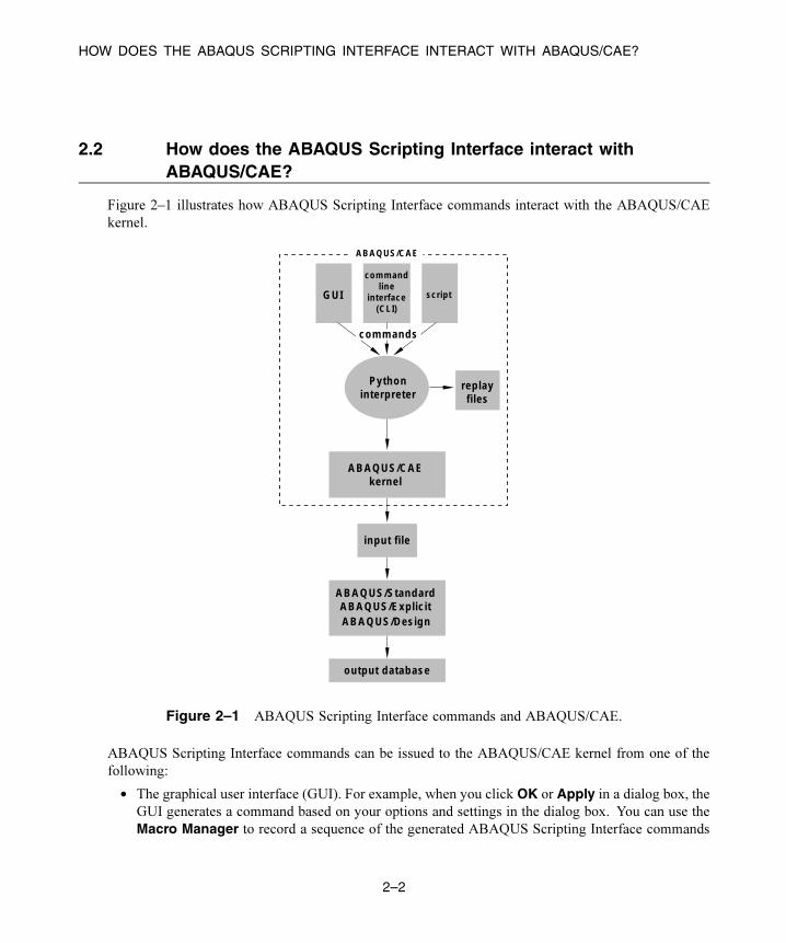
Figure 2–1 illustrates how ABAQUS Scripting Interface commands interact with the ABAQUS/CAE
kernel.
GUI
command�line�
interface�(CLI)
script
Python�interpreter
replay�files
ABAQUS/CAE�kernel
commands
input file
ABAQUS/Standard�ABAQUS/Explicit
output database
ABAQUS/CAE
�
�ABAQUS/Design
Figure 2–1 ABAQUS Scripting Interface commands and ABAQUS/CAE.
ABAQUS Scripting Interface commands can be issued to the ABAQUS/CAE kernel from one of the
following:
• The graphical user interface (GUI). For example, when you click OK or Apply in a dialog box, the
GUI generates a command based on your options and settings in the dialog box. You can use the
Macro Manager to record a sequence of the generated ABAQUS Scripting Interface commands
2–2

HOW DOES THE ABAQUS SCRIPTING INTERFACE INTERACT WITH ABAQUS/CAE?
in a macro file. For more information, see “Creating and running a macro,” Section 9.5.5 of the
ABAQUS/CAE User’s Manual.
• Click in the lower left corner of the main window to display the command line interface (CLI).
You can type a single command or paste in a sequence of commands from another window; the
command is executed when you press [Enter]. You can type any Python command into the command
line; for example, you can use the command line as a simple calculator.
Note: When you are using ABAQUS/CAE, errors and messages are posted into the message area.
Click in the lower left corner of the main window to display the message area.
• If you have more than a few commands to execute or if you are repeatedly executing the same
commands, it may be more convenient to store the set of statements in a file called a script. A
script contains a sequence of Python statements stored in plain ASCII format. For example, you
might create a script that opens an output database, displays a contour plot of a selected variable,
customizes the legend of the contour plot, and prints the resulting image on a local PostScript printer.
You can use one of the following methods to run a script:
Running a script when you start ABAQUS/CAE
You can run an ABAQUS/CAE script when you start a session by typing the following
command:
abaqus cae script=myscript.py
where myscript.py is the name of the file containing the script. The equivalent command
for ABAQUS/Viewer is
abaqus viewer script=myscript.py
Scripts are useful for starting ABAQUS/CAE in a predetermined state. For example,
you can define a standard configuration for printing, create remote queues, and define a set of
standard materials and their properties.
Running a script without the ABAQUS/CAE GUI
You can run a script without the ABAQUS/CAE GUI by typing the following command:
abaqus cae noGUI=myscript.py
where myscript.py is the name of the file containing the script. The equivalent command
for ABAQUS/Viewer is
abaqus viewer noGUI=myscript.py
The ABAQUS/CAE kernel is started without the GUI. Running a script without the
ABAQUS/CAE GUI is useful for automating pre- or postanalysis processing tasks without
the added expense of running a display. When the script finishes running, the ABAQUS/CAE
2–3

HOW DOES THE ABAQUS SCRIPTING INTERFACE INTERACT WITH ABAQUS/CAE?
kernel terminates. If you execute a script without the GUI, the script cannot interact with the
user, monitor jobs, or generate animations.
Running a script from the startup screen
When you start an ABAQUS/CAE session, ABAQUS displays the startup screen. You can run
a script from the startup screen by clicking Run Script. ABAQUS displays the Run Script
dialog box, and you select the file containing the script.
Running a script from the File menu
You can run a script by selecting File→Run Script from the main menu bar. ABAQUS
displays the Run Script dialog box, and you select the file containing the script.
Running a script from the command line interface
You can run a script from the command line interface (CLI) by typing the following command:
execfile('myscript.py')
where myscript.py is the name of the file containing the script and the file in this example
is in the current directory. Figure 2–2 shows an example script being run from the command
line interface.
Figure 2–2 Scripts can be run from the command line interface.
Click in the lower left corner of the main window to switch from the message area to the
command line interface.
2–4

CREATING A PART
3. Simple examples
Programming with the ABAQUS Scripting Interface is straightforward and logical. To illustrate how
easy it is to write your own programs, the following sections describe two simple ABAQUS Scripting
Interface scripts.
• “Creating a part,” Section 3.1
• “Reading from an output database,” Section 3.2
You are not expected to understand every line of the examples; the terminology and the syntax will
become clearer as you read the detailed explanations in the following chapters. “Summary,” Section 3.3,
describes some of the principles behind programming with Python and the ABAQUS Scripting Interface.
3.1 Creating a part
The first example shows how you can use an ABAQUS/CAE script to replicate the functionality of
ABAQUS/CAE. The script does the following:
• Creates a new model in the model database.
• Creates a two-dimensional sketch.
• Creates a three-dimensional, deformable part.
• Extrudes the two-dimensional sketch to create the first geometric feature of the part.
• Creates a new viewport.
• Displays a shaded image of the new part in the new viewport.
The new viewport and the shaded part are shown in Figure 3–1.
The example scripts from this manual can be copied to the user’s working directory by using the
ABAQUS fetch utility:
abaqus fetch job=scriptName
where scriptName.py is the name of the script (see “Execution procedure for ABAQUS/Fetch,”
Section 3.2.12 of the ABAQUS Analysis User’s Manual). Use the following command to retrieve the
script for this example:
abaqus fetch job=modelAExample
Note: ABAQUS does not install the sample scripts by default during the installation procedure. As
a result, if the ABAQUS fetch utility fails to find the sample script, the script may be missing from
your ABAQUS installation. You must rerun the installation procedure and request ABAQUS sampleproblems from the list of items to install.
3–1

CREATING A PART
Figure 3–1 The example creates a new viewport and a part.
To run the program, do the following:
1. Start ABAQUS/CAE by typing abaqus cae.
2. From the startup screen, select Run Script.
3. From the Run Script dialog box that appears, select modelAExample.py.
4. Click OK to run the script.
Note: If ABAQUS/CAE is already running, you can run the script by selecting File→Run Script from
the main menu bar.
3.1.1 The example script
"""modelAExample.py
A simple example: Creating a part."""
from abaqus import *from abaqusConstants import *import sketchimport part
3–2

CREATING A PART
myModel = mdb.Model(name='Model A')
mySketch = myModel.Sketch(name='Sketch A', sheetSize=200.0)
xyCoordsInner = ((-5 , 20), (5, 20), (15, 0),(-15, 0), (-5, 20))
xyCoordsOuter = ((-10, 30), (10, 30), (40, -30),(30, -30), (20, -10), (-20, -10),(-30, -30), (-40, -30), (-10, 30))
for i in range(len(xyCoordsInner)-1):mySketch.Line(point1=xyCoordsInner[i],
point2=xyCoordsInner[i+1])
for i in range(len(xyCoordsOuter)-1):mySketch.Line(point1=xyCoordsOuter[i],
point2=xyCoordsOuter[i+1])
myPart = myModel.Part(name='Part A', dimensionality=THREE_D,type=DEFORMABLE_BODY)
myPart.BaseSolidExtrude(sketch=mySketch, depth=20.0)
myViewport = session.Viewport(name='Viewport for Model A',origin=(10, 10), width=150, height=100)
myViewport.setValues(displayedObject=myPart)
myViewport.partDisplay.setValues(renderStyle=SHADED)
3.1.2 How does the script work?
This section explains each portion of the example script.
from abaqus import *
This statement makes the basic ABAQUS objects accessible to the script. It also provides access to a
default model database using the variable named mdb. The statement, from abaqusConstants
3–3

CREATING A PART
import *, makes the Symbolic Constants defined by the ABAQUS Scripting Interface available to
the script.
import sketchimport part
These statements provide access to the objects related to sketches and parts. sketch and part are
called Python modules.
The next statement in the script is shown in Figure 3–2. You can read this statement from right to
left as follows:
1. Create a new model named Model A.
2. Store the new model in the model database mdb.
3. Assign the new model to a variable called myModel.
myModel = mdb.Model(name='Model A')
1. Create a new model� named 'Model A'
2. Store the new model in the� model database mdb
3. Assign a variable� to the new model
Figure 3–2 Creating a new model.
mySketch = myModel.Sketch(name='Sketch A', sheetSize=200.0)
This statement creates a new sketch object named Sketch A in myModel. The variable mySketchis assigned to the new sketch. The sketch will be placed on a sheet 200 units square. Note the following:
• A command that creates something (an “object” in object-oriented programming terms) is called
a constructor and starts with an uppercase character. You have seen the Model and Sketchcommands that create Model objects and Sketch objects, respectively.
• The command uses the variable myModel that we created in the previous statement. Using
variables with meaningful names in a script makes the script easier to read and understand.
xyCoordsInner = ((-5 , 20), (5, 20), (15, 0),(-15, 0), (-5, 20))
xyCoordsOuter = ((-10, 30), (10, 30), (40, -30),(30, -30), (20, -10), (-20, -10),
3–4

CREATING A PART
(-30, -30), (-40, -30), (-10, 30))
These two statements define the X- and Y-coordinates of the vertices that form the inner and outer profile
of the letter “A.” The variable xyCoordsInner refers to the vertices of the inner profile, and the
variable xyCoordsOuter refers to the vertices of the outer profile.
for i in range(len(xyCoordsInner)-1):mySketch.Line(point1=xyCoordsInner[i],
point2=xyCoordsInner[i+1])
This loop creates the inner profile of the letter “A” in mySketch. Four lines are created using the X-
and Y-coordinates of the vertices in xyCoordsInner to define the beginning point and the end point
of each line. Note the following:
• Python uses only indentation to signify the start and the end of a loop. Python does not use the
brackets {} of C and C++.
• The len() function returns the number of coordinate pairs in xyCoordsInner—five in our
example.
• The range() function returns a sequence of integers. In Python, as in C and C++, the index of an
array starts at zero. In our example range(4) returns 0,1,2,3. For each iteration of the loop
in the example the variable i is assigned to the next value in the sequence of integers.
Similarly, a second loop creates the outer profile of the “A” character.
myPart = myModel.Part(name='Part A',dimensionality=THREE_D, type=DEFORMABLE_BODY)
This statement creates a three-dimensional, deformable part named Part A in myModel. The new part
is assigned to the variable myPart.
myPart.BaseSolidExtrude(sketch=mySketch, depth=20.0)
This statement creates a base solid extrude feature in myPart by extruding mySketch through a depth
of 20.0.
myViewport = session.Viewport(name='Viewport for Model A',origin=(20,20), width=150, height=100)
This statement creates a new viewport named Viewport for Model A in session. The new
viewport is assigned to the variable myViewport. The origin of the viewport is at (20, 20), and it has
a width of 150 and a height of 100.
3–5

READING FROM AN OUTPUT DATABASE
myViewport.setValues(displayedObject=myPart)
This statement tells ABAQUS to display the new part, myPart, in the new viewport, myViewport.
myViewport.partDisplayOptions.setValues(renderStyle=SHADED)
This statement sets the render style of the part display options in myViewport to shaded. As a result,
myPart appears in the shaded render style.
3.2 Reading from an output database
The second example shows how you can use the ABAQUS Scripting Interface to read an output database,
manipulate the data, and display the results using the Visualization module in ABAQUS/CAE. The
ABAQUS Scripting Interface allows you to display the data even though you have not written it back to
an output database. The script does the following:
• Opens the tutorial output database.
• Creates variables that refer to the first and second steps in the output database.
• Creates variables that refer to the last frame of the first and second steps.
• Creates variables that refer to the displacement field output in the last frame of the first and second
steps.
• Creates variables that refer to the stress field output in the last frame of the first and second steps.
• Subtracts the displacement field output from the two steps and puts the result in a variable called
deltaDisplacement.
• Subtracts the stress field output from the two steps and puts the result in a variable called
deltaStress.
• Selects deltaDisplacement as the default deformed variable.
• Selects the von Mises invariant of deltaStress as the default field output variable.
• Plots a contour plot of the result.
The resulting contour plot is shown in Figure 3–3.
Use the following commands to retrieve the script and the output database that is read by the script:
abaqus fetch job=odbExampleabaqus fetch job=viewer_tutorial
3.2.1 The example script
"""odbExample.py
3–6

READING FROM AN OUTPUT DATABASE
(Ave. Crit.: 75%)S - S, Mises
+7.679e-05+3.413e-03+6.750e-03+1.009e-02+1.342e-02+1.676e-02+2.010e-02+2.343e-02+2.677e-02+3.011e-02+3.344e-02+3.678e-02+4.012e-02
Step: Session Step, Step for Viewer non-persistent fieldsSession FramePrimary Var: S - S, MisesDeformed Var: U - U Deformation Scale Factor: +1.000e+00
DYNAMIC LOADING OF AN ELASTOMERIC, VISCOELASTICODB: viewer_tutorial.odb ABAQUS/Standard Wed Dec 31 19
1
2
3
Figure 3–3 The resulting contour plot.
Script to open an output database, superimpose variablesfrom the last frame of different steps, and display a contourplot of the result."""
from abaqus import *from abaqusConstants import *import visualization
myViewport = session.Viewport(name='Superposition example',origin=(10, 10), width=150, height=100)
# Open the tutorial output database.
myOdb = visualization.openOdb(path='viewer_tutorial.odb')
# Associate the output database with the viewport.
myViewport.setValues(displayedObject=myOdb)
# Create variables that refer to the first two steps.
firstStep = myOdb.steps['Step-1']
3–7

READING FROM AN OUTPUT DATABASE
secondStep = myOdb.steps['Step-2']
# Read displacement and stress data from the last frame# of the first two steps.
frame1 = firstStep.frames[-1]frame2 = secondStep.frames[-1]
displacement1 = frame1.fieldOutputs['U']displacement2 = frame2.fieldOutputs['U']
stress1 = frame1.fieldOutputs['S']stress2 = frame2.fieldOutputs['S']
# Find the added displacement and stress caused by# the loading in the second step.
deltaDisplacement = displacement2 - displacement1deltaStress = stress2 - stress1
# Create a Mises stress contour plot of the result.
myViewport.odbDisplay.setDeformedVariable(deltaDisplacement)
myViewport.odbDisplay.setPrimaryVariable(field=deltaStress,outputPosition=INTEGRATION_POINT,refinement=(INVARIANT, 'Mises'))
myViewport.odbDisplay.setPlotMode(CONTOUR)
3.2.2 How does the script work?
This section explains each portion of the example script.
from abaqus import *from abaqusConstants import *
These statements make the basic ABAQUS objects accessible to the script as well as all the Symbolic
Constants defined in the ABAQUS Scripting Interface.
3–8

READING FROM AN OUTPUT DATABASE
import visualization
This statement provides access to the commands that replicate the functionality of the Visualization
module in ABAQUS/CAE (ABAQUS/Viewer).
myViewport = session.Viewport(name='Superposition example')
This statement creates a new viewport named Superposition example in the session. The new
viewport is assigned to the variable myViewport. The origin and the size of the viewport assume the
default values.
odbPath = 'viewer_tutorial.odb'
This statement creates a path to the tutorial output database.
myOdb = session.openOdb(path=odbPath)
This statement uses the path variable odbPath to open the output database and to assign it to the variable
myOdb.
myViewport.setValues(displayedObject=myOdb)
This statement displays the default plot of the output database in the viewport.
firstStep = myOdb.steps['Step-1']secondStep = myOdb.steps['Step-2']
These statements assign the first and second steps in the output database to the variables firstStepand secondStep.
frame1 = firstStep.frames[-1]frame2 = secondStep.frames[-1]
These statements assign the last frame of the first and second steps to the variables frame1 andframe2.In Python an index of 0 refers to the first item in a sequence. An index of −1 refers to the last item in a
sequence.
displacement1 = frame1.fieldOutputs['U']displacement2 = frame2.fieldOutputs['U']
These statements assign the displacement field output in the last frame of the first and second steps to
the variables displacement1 and displacement2.
3–9

SUMMARY
stress1 = frame1.fieldOutputs['S']stress2 = frame2.fieldOutputs['S']
Similarly, these statements assign the stress field output in the last frame of the first and second steps to
the variables stress1 and stress2.
deltaDisplacement = displacement2 - displacement1
This statement subtracts the displacement field output from the last frame of the two steps and puts the
resulting field output into a new variable deltaDisplacement.
deltaStress = stress2 - stress1
Similarly, this statement subtracts the stress field output and puts the result in the variable
deltaStress.
myViewport.odbDisplay.setDeformedVariable(deltaDisplacement)
This statement uses deltaDisplacement, the displacement field output variable that we created
earlier, to set the deformed variable. This is the variable that ABAQUS will use to display the shape of
the deformed model.
myViewport.odbDisplay.setPrimaryVariable(field=deltaStress,outputPosition=INTEGRATION_POINT,refinement=(INVARIANT, 'Mises'))
This statement uses deltaStress, our stress field output variable, to set the primary variable. This is
the variable that ABAQUS will display in a contour or symbol plot.
myViewport.odbDisplay.setPlotMode(mode=CONTOUR)
The final statement sets the plot mode to display a contour plot.
3.3 Summary
The examples illustrate how a script can operate on a model in a model database or on the data stored in
an output database. The details of the commands in the examples are described in later sections; however,
you should note the following:
3–10

SUMMARY
• You can run a script from the ABAQUS/CAE startup screen when you start a session. After a
session has started, you can run a script from the File→Run Script menu or from the command
line interface.
• A script is a sequence of commands stored in ASCII format and can be edited with a standard text
editor.
• A set of example scripts are provided with ABAQUS. Use the abaqus fetch command to
retrieve a script and any associated files.
• You must use the import statement to make the required set of ABAQUS Scripting Interface
commands available. For example, the statement import part provides the commands that
create and operate on parts.
• A command that creates something (an “object” in object-oriented programming terms) is called a
constructor and starts with an uppercase character. For example, the following statement uses the
Model constructor to create a model object.
myModel = mdb.Model(name='Model A')
The model object created is
mdb.models['Model A']
• You can use a variable to refer to an object. Variables make your scripts easier to read and
understand. myModel refers to a model object in the previous example.
• A Python script can include a loop. The start and end of a loop is controlled by indentation in the
script.
• Python includes a set of built-in functions. For example, the len() function returns the length of
a sequence.
• You can use commands to replicate any operation that can be performed interactively when you
are working with ABAQUS/CAE; for example, creating a viewport, displaying a contour plot, and
setting the step and the frame to display.
3–11


Part II Using the ABAQUS Scripting Interface
This section provides an introduction to the Python programming language and a discussion of how you can
combine Python statements and the ABAQUS Scripting Interface to create your own scripts. The following
topics are covered:
• Chapter 4, “Introduction to Python”
• Chapter 5, “Using Python and the ABAQUS Scripting Interface”
• Chapter 6, “Using the ABAQUS Scripting Interface with ABAQUS/CAE”

PYTHON AND ABAQUS
4. Introduction to Python
This section provides a basic introduction to the Python programming language. You are encouraged to
try the examples and to experiment with Python statements. The Python language is used throughout
ABAQUS, not only in the ABAQUS Scripting Interface. Python is also used by ABAQUS/Design
to perform parametric studies and in the ABAQUS/Standard, ABAQUS/Explicit, and ABAQUS/CAE
environment file (abaqus_v6.env). For more information, see Part X, “Parametric Studies,” of the
ABAQUS Analysis User’s Manual, and “Using the ABAQUS environment settings,” Section 3.4.1 of
the ABAQUS Analysis User’s Manual.
The following topics are covered:
• “Python and ABAQUS,” Section 4.1
• “Python resources,” Section 4.2
• “Using the Python interpreter,” Section 4.3
• “Object-oriented basics,” Section 4.4
• “The basics of Python,” Section 4.5
• “Programming techniques,” Section 4.6
• “Further reading,” Section 4.7
4.1 Python and ABAQUS
Python is the standard programming language for ABAQUS products and is used in several ways.
• The ABAQUS environment file (abaqus_v6.env) uses Python statements.
• The parameter definitions on the data lines of the *PARAMETER option in the ABAQUS input file
are Python statements.
• The parametric study capability of ABAQUS requires the user to write and to execute a Python
scripting (.psf) file.
• ABAQUS/CAE records its commands as a Python script in the replay (.rpy) file.
• You can execute ABAQUS/CAE tasks directly using a Python script. You can execute a script from
ABAQUS/CAE using the following:
– File→Run Script from the main menu bar.
– The Macro Manager.
– The command line interface (CLI).
• You can access the output database (.odb) using a Python script.
4–1
PYTHON RESOURCES
4.2 Python resources
Python is an object-oriented programming language that is widely used in the software industry. A
number of resources are available to help you learn more about the Python programming language.
Python web sites
The official Python web site (www.python.org) contains a wealth of information on the Python
programming language and the Python community. For new Python programmers the web site
contains links to:
• General descriptions of the Python language.
• Comparisons between Python and other programming languages.
• An introduction to Python.
• Introductory tutorials.
The web site also contains a reference library of Python functions to which you will need to refer.
Python books
• Altom, Tim, Programming With Python, Prima Publishing, ISBN: 0761523340.
• Beazley, David, Python Essential Reference (2nd Edition), New Riders Publishing, ISBN:
0735710910.
• Brown, Martin, Python: The Complete Reference, McGraw-Hill, ISBN: 07212718X.
• Brown, Martin, Python Annotated Archives, McGraw-Hill, ISBN: 072121041.
• Chun, Wesley J., Core Python Programming, Prentice Hall, ISBN: 130260363.
• Deitel, Harvey M., Python: How to Program, Prentice Hall, ISBN: 130923613.
• Gauld, Alan, Learn To Program Using Python, Addison-Wesley, ISBN: 201709384.
• Harms, Daryl D., and Kenneth McDonald, Quick Python Book, Manning Publications
Company, ISBN: 884777740.
• Lie Hetland, Magnus, Practical Python, APress, ISBN: 1590590066.
• Lutz, Mark, Programming Python, O’Reilly & Associates, ISBN: 1565921976.
• Lutz, Mark, and David Ascher, Learning Python, Second Edition, O’Reilly & Associates,
ISBN: 0596002815.
• Lutz, Mark, and Gigi Estabrook, Python: Pocket Reference, O’Reilly & Associates, ISBN:
1565925009.
• Martelli, Alex, Python in a Nutshell, O’Reilly & Associates, ISBN: 0596001886.
• Martelli, Alex, and David Ascher, Python Cookbook, O’Reilly & Associates, ISBN:
0596001673.
• Van Laningham, Ivan, Sams Teach Yourself Python in 24 Hours, Sams Publishing, ISBN:
0672317354.
4–2
USING THE PYTHON INTERPRETER
The books Python Essential Reference and Learning Python are recommended reading.
Python newsgroups
Discussions of Python programming can be found at:
• comp.lang.python
• comp.lang.python.announce
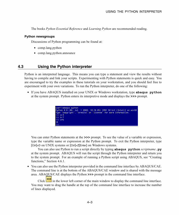
4.3 Using the Python interpreter
Python is an interpreted language. This means you can type a statement and view the results without
having to compile and link your scripts. Experimenting with Python statements is quick and easy. You
are encouraged to try the examples in these tutorials on your workstation, and you should feel free to
experiment with your own variations. To run the Python interpreter, do one of the following:
• If you have ABAQUS installed on your UNIX or Windows workstation, type abaqus pythonat the system prompt. Python enters its interpretive mode and displays the >>> prompt.
You can enter Python statements at the >>> prompt. To see the value of a variable or expression,
type the variable name or expression at the Python prompt. To exit the Python interpreter, type
[Ctrl]+D on UNIX systems or [Ctrl]+Z[Enter] on Windows systems.
You can also use Python to run a script directly by typing abaqus python scriptname.pyat the system prompt. ABAQUS will run the script through the Python interpreter and return you
to the system prompt. For an example of running a Python script using ABAQUS, see “Creating
functions,” Section 4.6.1.
• You can also use the Python interpreter provided in the command line interface by ABAQUS/CAE.
The command line is at the bottom of the ABAQUS/CAE window and is shared with the message
area. ABAQUS/CAE displays the Python >>> prompt in the command line interface.
Click in the lower left corner of the main window to display the command line interface.
You may want to drag the handle at the top of the command line interface to increase the number
of lines displayed.
4–3

OBJECT-ORIENTED BASICS
If ABAQUS/CAE displays new messages while you are using the command line interface, the
message area tab turns red.
4.4 Object-oriented basics
You need to understand some of the fundamentals of object-oriented programming to understand the
terms used in this manual. The following is a brief introduction to the basic concepts behind object-
oriented programming.
Traditional procedural languages, such as FORTRAN and C, are based around functions or
subroutines that perform actions. A typical example is a subroutine that calculates the geometric center
of a planar part given the coordinates of each vertex.
In contrast, object-oriented programming languages, such as Python and C++, are based around
objects. An object encapsulates some data and functions that are used to manipulate those data. The data
encapsulated by an object are called the members of the object. The functions that manipulate the data
are called methods.
An object can be modeled from a real-world object, such as a tire; or an object can be modeled from
something more abstract, such as an array of nodes. For example, the data (or members) encapsulated by
a tire object are its diameter, width, aspect ratio, and price. The functions or methods encapsulated by the
tire object calculate how the tire deforms under load and how it wears during use. Members and methods
can be shared by more than one type of object; for example, a shock absorber has a price member and a
deformation method.
Classes are an important concept in object-oriented programming. Classes are defined by the
programmer, and a class defines members and the methods that operate on those members. An object
is an instance of a class. An object inherits the members and methods of the class from which it was
instanced. You should read a Python text book for a thorough discussion of classes, abstract base
classes, and inheritance.
4–4
THE BASICS OF PYTHON
4.5 The basics of Python
The following sections introduce you to the basics of the Python language. The following topics are
covered:
• “Variable names and assignment,” Section 4.5.1
• “Python data types,” Section 4.5.2
• “Determining the type of a variable,” Section 4.5.3
• “Sequences,” Section 4.5.4
• “Sequence operations,” Section 4.5.5
• “Python None,” Section 4.5.6
• “Continuation lines and comments,” Section 4.5.7
• “Printing variables using formatted output,” Section 4.5.8
• “Control blocks,” Section 4.5.9
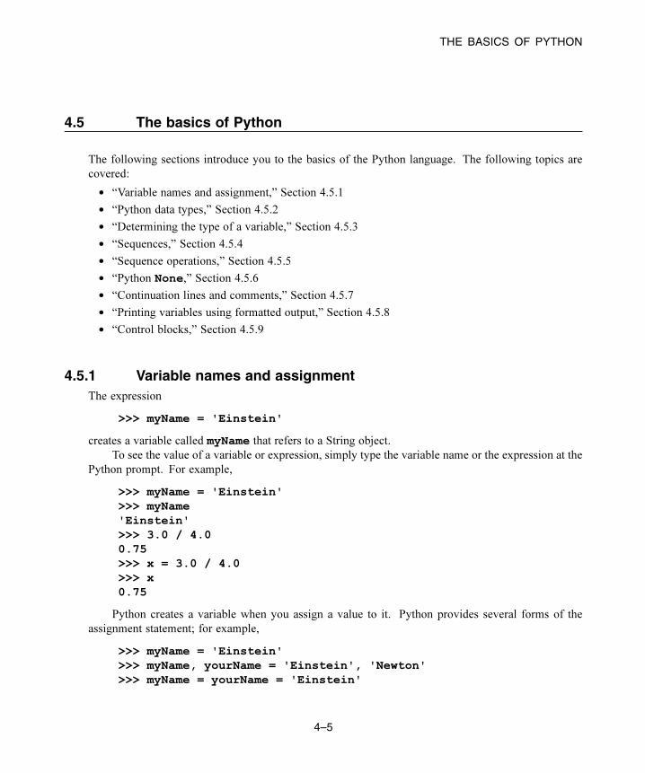
4.5.1 Variable names and assignment
The expression
>>> myName = 'Einstein'
creates a variable called myName that refers to a String object.
To see the value of a variable or expression, simply type the variable name or the expression at the
Python prompt. For example,
>>> myName = 'Einstein'>>> myName'Einstein'>>> 3.0 / 4.00.75>>> x = 3.0 / 4.0>>> x0.75
Python creates a variable when you assign a value to it. Python provides several forms of the
assignment statement; for example,
>>> myName = 'Einstein'>>> myName, yourName = 'Einstein', 'Newton'>>> myName = yourName = 'Einstein'
4–5

THE BASICS OF PYTHON
The second line assigns the string ’Einstein’ to the variable myName and assigns the string
’Newton’ to the variable yourName. The third line assigns the string ’Einstein’ to both
myName and yourName.The following naming rules apply:
• Variable names must start with a letter or an underscore character and can contain any number of
letters, digits, or underscores. load_3 and _frictionStep are legal variable names; 3load,load_3$, and $frictionStep are not legal names. There is no limit on the length of a variable
name.
• Some words are reserved and cannot be used to name a variable; for example, print, while,return, and class.
• Python is case sensitive. A variable named Load is different from a variable named load.
When you assign a variable in a Python program, the variable refers to a Python object, but the
variable is not an object itself. For example, the expression numSpokes=3 creates a variable that refers
to an integer object; however, numSpokes is not an object. You can change the object to which a
variable refers. numSpokes can refer to a real number on one line, an integer on the next line, and a
viewport on the next line.
The first example script in “Creating a part,” Section 3.1, created a model using the following
statement:
myModel = mdb.Model(name='Model A')
The constructor mdb.Model(name=’Model A’) creates an instance of a model, and this instance is
a Python object. The object created is mdb.models[’Model A’], and the variable myModel refers
to this object.
An object always has a type. In our example the type of mdb.models[’Model A’] is
Model. An object’s type cannot be changed. The type defines the data encapsulated by an object—its
members—and the functions that can manipulate those data—its methods. Unlike most programming
languages, you do not need to declare the type of a variable before you use it. Python determines
the type when the assignment statement is executed. The ABAQUS Scripting Interface uses the term
“object” to refer to a specific ABAQUS type as well as to an instance of that type; for example, a
Model object refers to a Model type and to an instance of a Model type.
4.5.2 Python data types
Python includes the following built-in data types:
Integer
To create variables called “i” and “j” that refer to integer objects, type the following at the Python
prompt:
>>> i = 20>>> j = 64
4–6

THE BASICS OF PYTHON
An integer is based on a C long and can be compared to a FORTRAN integer*4 or *8. For extremely
large integer values, you should declare a long integer. The size of a long integer is essentially
unlimited. The “L” at the end of the number indicates that it is a long integer.
>>> nodes = 2000000L>>> bigNumber = 120L**21
Use int(n) to convert a variable to an integer; use long(n) to convert a variable to a long integer.
>>> load = 279.86>>> iLoad = int(load)>>> iLoad279
>>> a = 2>>> b = 64>>> bigNumber = long(a)**b>>> print 'bigNumber = ', bigNumberbigNumber = 18446744073709551616
Note: All ABAQUS Scripting Interface object types begin with an uppercase character; for
example, a Part or a Viewport. An integer is another kind of object and follows the same
convention. The ABAQUS Scripting Interface refers to an integer object as an “Int.” Similarly, the
ABAQUS Scripting Interface refers to a floating-point object as a “Float.”
Float
Floats represent floating-point numbers or real numbers. You can use exponential notation for floats.
>>> pi = 22.0/7.0>>> r = 2.345e-6>>> area = pi * r * r>>> print 'Area = ', areaArea = 1.728265e-11
A float is based on a C double and can be compared to a FORTRAN real*8. Use float(n) to
convert a variable to a float.
Complex
Complex numbers use the “j” notation to indicate the imaginary part of the number. Python provides
methods to manipulate complex numbers. The conjugate method calculates the conjugate of a
complex number.
>>> a = 2 + 4j>>> a.conjugate()(2-4j)
4–7

THE BASICS OF PYTHON
A complex number has two members, the real member and the imaginary member.
>>> a = 2 + 4j>>> a.real2.0>>> a.imag4.0
Python provides complex math functions to operate on complex variables. You need to import the
cmath module to use the complex square root function.
>>> import cmath>>> y = 3 + 4j>>> print cmath.sqrt(y)(2+1j)
Remember, functions of a type are calledmethods; data of a type are calledmembers. In our example
conjugate is a method of a complex type; a.real refers to the real member of a complex type.
Sequences
Sequences include strings, lists, tuples, and arrays. Sequences are described in “Sequences,”
Section 4.5.4, and “Sequence operations,” Section 4.5.5.
4.5.3 Determining the type of a variable
You use the type() function to return the type of the object to which a variable refers.
>>> a = 2.375>>> type(a)<type 'float'>>>> a = 1>>> type(a)<type 'int'>>>> a = 'chamfer'>>> type(a)<type 'string'>
4.5.4 Sequences
Sequences are important and powerful data types in Python. A sequence is an object containing a
series of objects. There are three types of built-in sequences in Python—list, tuple, and string. In
addition, imported modules allow you to use arrays in your scripts. The following table describes the
characteristics of list, tuple, string, and array sequences.
4–8
THE BASICS OF PYTHON
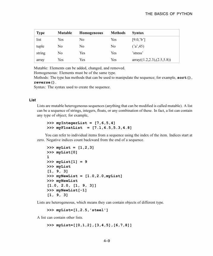
Type Mutable Homogeneous Methods Syntax
list Yes No Yes [9.0,’b’]
tuple No No No (’a’,45)
string No Yes Yes ’stress’
array Yes Yes Yes array((1.2,2.3),(2.5,5.8))
Mutable: Elements can be added, changed, and removed.
Homogeneous: Elements must be of the same type.
Methods: The type has methods that can be used to manipulate the sequence; for example, sort(),reverse().Syntax: The syntax used to create the sequence.
List
Lists are mutable heterogeneous sequences (anything that can be modified is called mutable). A list
can be a sequence of strings, integers, floats, or any combination of these. In fact, a list can contain
any type of object; for example,
>>> myIntegerList = [7,6,5,4]>>> myFloatList = [7.1,6.5,5.3,4.8]
You can refer to individual items from a sequence using the index of the item. Indices start at
zero. Negative indices count backward from the end of a sequence.
>>> myList = [1,2,3]>>> myList[0]1>>> myList[1] = 9>>> myList[1, 9, 3]>>> myNewList = [1.0,2.0,myList]>>> myNewList[1.0, 2.0, [1, 9, 3]]>>> myNewList[-1][1, 9, 3]
Lists are heterogeneous, which means they can contain objects of different type.
>>> myList=[1,2.5,'steel']
A list can contain other lists.
>>> myList=[[0,1,2],[3,4,5],[6,7,8]]
4–9

THE BASICS OF PYTHON
>>> myList[0][0, 1, 2]>>> myList[2][6,7,8]
myList[1][2] refers to the third item in the second list. Remember, indices start at zero.
>>> myList[1][2]5
Python has built-in methods that allow you to operate on the items in a sequence.
>>> myList[1, 9, 3]>>> myList.append(33)>>> myList[1, 9, 3, 33]>>> myList.remove(9)>>> myList[1, 3, 33]
The following are some additional built-in methods that operate on lists:
count()
Return the number of times a value appears in the list.
>>> myList = [0,1,2,1,2,3,2,3,4,3,4,5]>>> myList.count(2)3
index()
Return the index indicating the first time an item appears in the list.
>>> myList.index(5)11>>> myList.index(4)8
insert()
Insert a new element into a list at a specified location.
>>> myList.insert(2,22)>>> myList[0, 1, 22, 2, 1, 2, 3, 2, 3, 4, 3, 4, 5]
4–10

THE BASICS OF PYTHON
reverse()
Reverse the elements in a list.
>>> myList.reverse()>>> myList[5, 4, 3, 4, 3, 2, 3, 2, 1, 2, 22, 1, 0]
sort()
Sort the elements in a list.
>>> myList.sort()>>> myList[0, 1, 1, 2, 2, 2, 3, 3, 3, 4, 4, 5, 22]
Tuple
Tuples are very similar to lists; however, they are immutable heterogeneous sequences, whichmeans
that you cannot change them after you create them. You can think of a tuple as a list that cannot be
modified. Tuples have no methods; you cannot append items to a tuple, and you cannot modify or
delete the items in a tuple. The following statement creates an empty tuple:
myTuple = ()
The following statement creates a tuple with one element:
myTuple = (5.675,)
You can use the tuple() function to convert a list or a string to a tuple.
>>> myList = [1, 2, "stress", 4.67]>>> myTuple = tuple(myList)>>> print myTuple(1, 2, 'stress', 4.67)>>> myString = 'Failure mode'>>> myTuple = tuple(myString)>>> print myTuple('F', 'a', 'i', 'l', 'u', 'r', 'e', ' ', 'm', 'o', 'd', 'e')
The following statements create a tuple and then try to change the value of an item in the tuple.
An AttributeError error message is generated because a tuple is immutable.
>>> myTuple = (1,2,3,4,5)>>> type(myTuple)<type 'tuple'>>>> myTuple[2]=3Traceback (innermost last):
4–11

THE BASICS OF PYTHON
File "", line 1, in ?AttributeError: __setitem__
String
Strings are immutable sequences of characters. Strings are defined by single or double quotation
marks. You can use the “+” operator to concatenate two strings and create a third string; for example,
>>> odbString = "Symbol plot from ">>> odb = 'load1.odb'>>> annotationString = odbString + odb>>> print annotationStringSymbol plot from load1.odb
Note: You can also use the “+” operator to concatenate tuples and lists.
Python provides a set of functions that operate on strings.
>>> annotationString'Symbol plot from load1.odb'>>> annotationString.upper()'SYMBOL PLOT FROM LOAD1.ODB'>>> annotationString.split()['Symbol', 'plot', 'from', 'load1.odb']
As with all sequences, you use negative indices to index backward from the end of a string.
>>> axis_label = 'maxstrain'>>> axis_label[-1]'n'
Use the built-in str function to convert an object to a string.
>>> myList = [8, 9, 10]>>> str(myList)'[8, 9, 10]'
Look at the standard Python documentation on the official Python web site (www.python.org) for
a list of common string operations. String functions are described in the String Servicessection of the Python Library Reference.
Array
Arrays are mutable homogeneous sequences. The Numeric module allows you to create and
operate on multidimensional arrays. Python determines the type of elements in the array; you do
not have to declare the type when you create the array.
>>> from Numeric import array>>> myIntegerArray = array([[1,2],[2,3],[3,4]])
4–12

THE BASICS OF PYTHON
>>> myIntegerArrayarray([[1, 2],
[2, 3],[3, 4]])
>>> myRealArray =array([[1.0,2],[2,3],[3,4]])>>> myRealArrayarray([[1., 2.],
[2., 3.],[3., 4.]])
>>> myRealArray * myIntegerArrayarray([[ 1., 4.],
[ 4., 9.],[ 9., 16.]])
Arrays have methods. To find the methods of an object, type objectname followed by a period,
followed by two underscore characters, followed by methods, followed by two more underscore
characters. For example,
>>> myArray=array(((1,3),(2,4),(3,5)))>>> myArray.__methods__['__copy__', 'astype', 'byteswapped', 'iscontiguous','itemsize', 'tolist', 'tostring', 'typecode']
4.5.5 Sequence operations
Python provides a set of tools that allow you to operate on a sequence.
Slicing
Sequences can be divided into smaller sequences. This operation is called slicing. The expression
sequence[m:n] returns a copy of sequence fromm to n−1. The default value form is zero; the default
value for n is the length of the sequence.
>>> myList = [0,1,2,3,4]>>> myList[1:4][1, 2, 3]
>>> myString ='linear load'>>> myString[7:]'load'>>> myString[:6]'linear'
4–13

THE BASICS OF PYTHON
Repeat a sequence
>>> x=(1,2)>>> x*2(1, 2, 1, 2)>>> s = 'Hoop Stress'>>> s*2>>> 'Hoop StressHoop Stress'
Determine the length of a sequence
>>> myString ='linear load'>>> len(myString)11>>> myList = [0,1,2,3,4]>>> len(myList)5
Concatenate sequences
>>> a = [0,1]>>> b = [9,8]>>> a + b[0, 1, 9, 8]>>> test = 'wing34'>>> fileExtension = '.odb'>>> test+fileExtension'wing34.odb'
Range
The range() function generates a list containing a sequence of integers. You can use the
range() function to control iterative loops. The arguments to range are start (the starting
value), end (the ending value plus one), and step (the step between each value). The start and step
arguments are optional; the default start argument is 0, and the default step argument is 1. The
arguments must be integers.
>>> range(2,8)[2, 3, 4, 5, 6, 7]>>> range(4)[0, 1, 2, 3]>>> range(1,8,2)[1, 3, 5, 7]
4–14

THE BASICS OF PYTHON
Convert a sequence type
Convert a sequence to a list or a tuple.
>>> myString='noise'>>> myList = list(myString) #Convert a string to a list.>>> myList[0] = 'p'>>> myList['p', 'o', 'i', 's', 'e']>>> myTuple = tuple(myString) #Convert a string to a tuple.>>> print myTuple('n', 'o', 'i', 's', 'e')
4.5.6 Python None
Python defines a special object called the None object or “Python None” that represents an empty value.
The None object is returned by functions and methods that do not have a return value. The None object
has no value and prints as None. For example
>>> a = [1, 3, 7, 5]>>> print a.sort()None>>> import sys>>> x = sys.path.append('.')>>> print xNone
4.5.7 Continuation lines and comments
You can continue a statement on the following line if you break the statement between a set of (), {}, or
[] delimiters. For example, look at the tuple that was used in “Creating a part,” Section 3.1, to assign the
coordinates of the vertices to a variable:
xyCoordsOuter = ((-10, 30), (10, 30), (40, -30),(30, -30), (20, -10), (-20, -10),(-30, -30), (-40, -30), (-10, 30))
If a statement breaks at any other place, you must include a “\” character at the end of the line to indicate
that it is continued on the next line. For example,
distance = mdb.models['Model-1'].parts['housing'].\getDistance(entity1=node1, entity2=node2)
4–15

THE BASICS OF PYTHON
When you are running Python from a local UNIX or Windows window, the prompt changes to the “. . .”
characters to indicate that you are on a continuation line.
Comments in a Python script begin with the “#” character and continue to the end of the line.
>>> #Define material constants>>> modulus = 1e6 #Define Young's modulus
4.5.8 Printing variables using formatted output
Python provides a print function that displays the value of a variable. For example,
>>> freq = 22.0/7.0>>> x = 7.234>>> print 'Vibration frequency = ', freqVibration frequency = 3.14285714286>>> print 'Vibration frequency = ', freq, 'Displacement =\... ', xVibration frequency = 3.14285714286 Displacement = 7.234
The string modulus operator % allows you to format your output. The %s operator in the following
example converts the variables to strings.
>>> print 'Vibration frequency = %s Displacement =\... %s' % (freq, x)Vibration frequency = 3.14285714286 Displacement = 7.234
The %f operator specifies floating point notation and indicates the total number of characters to print and
the number of decimal places.
>>> print 'Vibration frequency = %6.2f Displacement =\... %6.2f' % (freq, x)Vibration frequency = 3.14 Displacement = 7.23
The %E operator specifies scientific notation and indicates the number of decimal places.
>>> print 'Vibration frequency = %.6E Displacement =\... %.2E' % (freq, x)Vibration frequency = 3.142857E+00 Displacement = 7.23E+00
The following list includes some additional useful printing operators.
• The + flag indicates that a number should include a sign.
• The \n escape sequence inserts a new line.
• The \t escape sequence inserts a tab character.
For example,
4–16

THE BASICS OF PYTHON
>>> print 'Vibration frequency = %+.6E\nDisplacement =\... %+.2E' % (freq, x)Vibration frequency = +3.142857E+00Displacement = +7.23E+00
4.5.9 Control blocks
Python does not use a special character, such as “}”, to signify the end of a control block such as an
if statement. Instead, Python uses indentation to indicate the end of a control block. You define the
indentation that governs a block. When your script returns to the original indentation, the block ends.
For example,
max = 5i = 0while i <= max:
square = i**2cube = i**3print i, square, cubei = i + 1
print 'Loop completed'
When you are using the Python interpreter from the ABAQUS/CAE command line interface or if
you are running Python from a local UNIX or Windows window, the prompt changes to the “. . .”
characters to indicate that you are in a block controlled by indentation.
if, elif, and else
>>> load = 10>>> if load > 6.75:... print 'Reached critical load'... elif load < 2.75:... print 'Minimal load'... else:... print 'Typical load'
while
>>> load = 10>>> length = 3>>> while load < 1E4:... load = load * length... print load
Use break to break out of a loop.
4–17

PROGRAMMING TECHNIQUES
>>> while 1:... x = raw_input(Enter a number or 0 to quit:')... if x == '0':... break... else:... print x
Use continue to skip the rest of the loop and to go to the next iteration.
>>> load = 10>>> length = -3>>> while load < 1E6: #Continue jumps up here... load = load * length... if load < 0:... continue #Do not print if negative... print load
for
Use a sequence to control the start and the end of for loops. The range() function is an easy
way to create a sequence.
>>> for i in range(5):... print i...01234
4.6 Programming techniques
The following sections introduce you to some of the techniques you will need to program with Python.
The following topics are covered:
• “Creating functions,” Section 4.6.1
• “Using dictionaries,” Section 4.6.2
• “Reading and writing from files,” Section 4.6.3
• “Error handling,” Section 4.6.4
4–18

PROGRAMMING TECHNIQUES
• “Functions and modules,” Section 4.6.5
• “Writing your own modules,” Section 4.6.6
4.6.1 Creating functions
You can define your own functions in Python. A function is like a subroutine in FORTRAN. You can
pass arguments into a function, it performs the operation, and it can return one or more values. For
example, the following function returns the distance of a point from the origin. The def statement starts
a function definition.
def distance(x, y):a = x**2 + y**2return a ** 0.5
You supply the arguments to a function in parentheses; for example,
>>> distance(4.7, 9.1)10.2420701033
You can assign the return value to a variable:
>>> d = distance(4.7, 9.1)>>> print d10.2420701033
One of the methods provided by ABAQUS uses as many as 50 arguments. Some of the arguments
are required by the method; others are optional, and ABAQUS provides an initial or default value.
Fortunately, you can call a function or a method without providing every optional argument if you use
Python’s “keyword” arguments. A keyword specifies the argument that you are providing. Keyword
arguments also make your scripts more readable. For example, the following defines a function called
calculateCylinderVolume:
>>> from math import *>>> def calculateCylinderVolume(radius,height):... volume = pi * radius**2 * height... return volume
You can call the function with the following line:
>>> volume = calculateCylinderVolume(3.2,27.5)
Here the arguments are called positional arguments because you are relying on their position in the
function call to determine the variable to which they are assigned in the function—radius followed by
height.
4–19

PROGRAMMING TECHNIQUES
The following is the same statement using keyword arguments:
>>> volume = calculateCylinderVolume(radius=3.2, height=27.5)
Keyword arguments make your code more readable. In addition, if you use keyword arguments, you can
enter the arguments in any order.
>>> volume = calculateCylinderVolume(height=27.5, radius=3.2)
You can define default values for an argument in a function definition. For example, the following
sets the default value of radius to 0.5 and the default value of height to 1.0:
>>> from math import *>>> def calculateCylinderVolume(radius=0.5,height=1.0):... volume = pi * radius * radius * height... return volume
You can now call the function without providing all the arguments. The function assigns the default
value to any missing arguments.
>>> volume = calculateCylinderVolume(height=27.5)
It is good programming practice to use a documentation string that indicates the purpose of a
function and the arguments expected. A documentation string appears at the top of a function and is
delimited by triple quotes """. You can use the __doc__ method to obtain the documentation string
from a function while running the Python interpreter. For example,
>>>def calculateCylinderVolume(radius=0.5,height=1.0):... """... Calculates the volume of a cylinder....... Takes two optional arguments, radius (default=0.5)... and height (default=1.0).... """... from math import *... volume = pi * radius**2 * height... return volume...>>> print calculateCylinderVolume.__doc__
Calculates the volume of a cylinder.
Takes two optional arguments, radius (default=0.5)and height (default=1.0).
4–20
PROGRAMMING TECHNIQUES
You can retrieve the documentation string for the methods in the ABAQUS Scripting Interface. For
example,
>>> mdb.Model.__doc__'Mdb.Model(name <, description, stefanBoltzmann, absoluteZero>) ->
This method creates a Model object.'
>>> session.Viewport.__doc__'Session.Viewport(name <, origin, width, height, border, titleBar,
titleStyle, customTitleString>)-> This method creates a Viewport object with the specified
origin and dimensions.'
The documentation string shows the name of each argument name and whether the argument is required
or optional. The string also shows a brief description of the method.
You can use the sys module to retrieve command line arguments and pass them to a function. For
example, the following script takes two arguments—the X- and Y-coordinates of a point—and calculates
the distance from the point to the origin. The script uses the following modules:
• The sys module to retrieve the command line arguments.
• The math module to calculate the square root.
import sys, math#~~~~~~~~~~~~~~~~~~~~~~~~~~~~~~~~~~~~~~~~~def distance(x, y):
"""Prints distance from origin to (x, y).
Takes two command line arguments, x and y."""
# Square the arguments and add them.
a = x**2 + y**2
# Return the square root.
return math.sqrt(a)
# Retrieve the command line arguments and# convert the strings to floating-point numbers.
x = float(sys.argv[1])
4–21
PROGRAMMING TECHNIQUES
y = float(sys.argv[2])
# Call the distance function.
d = distance(x, y)
# Print the result.
print 'Distance to origin = ', d
To use this script, do the following:
• Copy the statements into a file called distance.py in your local directory.
• Type the following at the system prompt:
abaqus python distance.py 30 40
ABAQUS executes the script and prints the result.
Distance to origin = 50.0
4.6.2 Using dictionaries
Dictionaries are a powerful tool in Python. A dictionary maps a variable to a set of data, much like a real
dictionary maps a word to its definition, its pronunciation, and its synonyms. Dictionaries are similar to
lists in that they are not homogeneous and can contain objects of any type. To access an object in a list,
you provide the integer index that specifies the position of the object in the list. For example,
>>> myList = [6,2,9]>>> myList[1]2
In contrast, you access an object in a dictionary through its key, which can be a string, an integer, or anytype of immutable Python object. There is no implicit order to the keys in a dictionary. In most cases
you will assign a string to the dictionary key. The key then becomes a more intuitive way to access the
elements in a dictionary. You use square brackets and the dictionary key to access a particular object.
For example,
>>> myPart = {} #Create an empty dictionary>>> myPart['size'] = 3.0>>> myPart['material'] = 'Steel'>>> myPart['color'] = 'Red'>>> myPart['number'] = 667
You can add dictionary keys at any time.
4–22

PROGRAMMING TECHNIQUES
>>> myPart['weight'] = 376.0>>> myPart['cost'] = 10.34
You use the key to access an item in a dictionary.
>>> costOverWeight = myPart['cost'] / myPart['weight']>>> costOverWeight0.0275>>> description = myPart['color'] + myPart['material']>>> description'RedSteel'
Dictionaries are not sequences, and you cannot apply sequencemethods such as slicing and concatenating
to dictionaries. Dictionaries have their own methods. The following statement lists the methods of the
dictionary myPart.
>>> myPart.__methods__['clear', 'copy', 'get', 'has_key', 'items', 'keys','update', 'values']
The keys() method returns a list of the dictionary keys.
>>> myPart.keys()['size', 'weight', 'number', 'material', 'cost', 'color']
The values() method returns a list of the values of each entry in the dictionary.
>>> myPart.values()[3.0, 376.0, 667, 'Steel', 10.34, 'Red']
The items() method returns a list of tuples. Each tuple contains the key and its value.
>>> myPart.items()[('size', 3.0), ('number', 667), ('material', 'Steel'),('color', 'Red'), ('weight', 376.0), ('cost', 10.34),]
You use the has_key() method to see if a key exists. A return value of 1 indicates the key exists in
the dictionary. A return value of 0 indicates the key does not exist.
>>> myPart.has_key('color')1
Python’s del statement allows you to delete a variable.
>>> del myPart
You can also use del to delete an item from a dictionary.
>>> del myPart['color']
4–23

PROGRAMMING TECHNIQUES
>>> myPart.has_key('color')0
You can use the keys(), values(), or items() methods to loop through a dictionary. In the
following example, items() returns two values; the first is assigned to property, and the second is
assigned to setting.
>>> for property, setting in myPart.items():... print property, setting...size 3.0weight 376.0number 667material Steelcost 10.34
4.6.3 Reading and writing from files
Many of the file commands are built-in Python commands. You do not have to import a module to use
file commands. You use the open() function to create a file.
>>> myInputFile = open('crash_test/fender.txt','r')>>> myOutputFile = open('peak_deflection.txt','w+')
The first line opens an existing file in the crash_test directory called fender.txt. The file is
opened in read-only mode; myInputFile is a variable that refers to a file object. The second line
creates and opens a new file object in the local directory called peak_deflection.txt. This file isopened in read and write mode.
Use the “__methods__” technique that we saw earlier to see the methods of a file object.
>>> myOutputFile = open('peak_deflection.txt','w')>>> myOutputFile.__methods__['close', 'fileno', 'flush', 'isatty', 'read','readinto', 'readline', 'readlines', 'seek', 'tell','truncate', 'write', 'writelines']
The readline() method reads a single line from a file into a string, including the new line character
that terminates the string. The readlines() method reads all the lines in a file into a list. The
write() function writes a string to a file. Look at the standard Python documentation on the official
Python web site (www.python.org) for a description of functions that operate on files. File objects are
described in the Built-in Types section of the Python Library Reference.The following example reads each line of a text file and changes the line to uppercase characters:
# Read-only is the default access mode
4–24

PROGRAMMING TECHNIQUES
>>> inputFile = open('foam.txt')
# You must declare write access
>>> outputFile = open('upper.txt','w')>>> lines = inputFile.readlines()>>> for line in lines:... newLine = line.upper()... outputFile.write(newLine)...>>> inputFile.close()>>> outputFile.close()
The first line opens the input file; you don’t need the ’r’ because read-only is the default access mode.
The next line opens a new file to which you will write. You read the lines in the input file into a list.
Finally, you enter a loop that converts each line to uppercase characters and writes the result to the output
file. The final two lines close the files.
4.6.4 Error handling
When a script encounters unusual circumstances, Python allows you tomodify the flow of control through
the script and to take the necessary action. The action of signaling a problem during execution is called
raising or throwing an exception. Recognizing the problem is called catching an exception. Taking
appropriate action is called exception handling.
Python provides exception handling through the try and except commands. For example, the
following statement attempts to open an existing file for reading:
>>> outputFile = open('foam.txt')
If the file does not exist, the statement fails, and Python displays the following error message:
>>> outputFile = open('foam.txt')Traceback (innermost last):
File "<stdin>", line 1, in ?IOError: (2, 'No such file or directory')
If you use exception handling, you can catch the error, display a helpful message, and take the appropriate
action. For example, a revised version of the code attempts to open the same file within a try statement.
If an IOError error is encountered, the except statement catches the IOError exception and assigns
the exception’s value to the variable error.
>>> try:... outputFile = open('foam.txt')
4–25

PROGRAMMING TECHNIQUES
... except IOError,error:
... print 'Exception trapped: ', error
...Exception trapped: (2, 'No such file or directory')
You can raise your own exceptions by providing the error type and the error message to the raisestatement. The following example script raises an exception and displays a message if the function
myFunction encounters a problem.
def myFunction(x,y):
if y == 0:raise ValueError, 'y argument cannot be zero'
else:return x/y
try:print myFunction(temperature, velocity)
except ValueError, error:print error
Exception handling is discussed in more detail in “Error handling in the ABAQUS Scripting Interface,”
Section 5.5.
4.6.5 Functions and modules
When you start Python from a local window or from ABAQUS/CAE, the Python interpreter is aware of
a limited set of built-in functions. For example, try entering the following at the Python prompt:
>>> myName = 'Einstein'>>> len(myName)
Python returns the number 8, indicating the length of the string myName. The len() function is a
built-in function and is always available when you are using Python. To see a list of the built-in functions
provided by Python, type dir(__builtins__) at the Python prompt.
Note: dir(__builtins__) is typed as dir(“underscore underscore”builtins“underscore
underscore”). You have seen this “underscore underscore” notation already in “Sequences,”
Section 4.5.4.
In addition, you can look at the standard Python documentation on the official Python web site
(www.python.org) for a list of built-in functions. Built-in functions are described in the Built-inFunctions section of the Python Library Reference.
4–26

PROGRAMMING TECHNIQUES
Many functions, however, are not built-in; for example, most of the math functions, such as
sin() and cos(), are not available when you start Python. Functions that are not built-in are defined
in modules. Modules are a way of grouping functionality and are similar to a FORTRAN library of
subroutines. For example, the following code could be the opening lines of a Python script. The
code imports the Python module sys and uses the argv member of sys to print the command line
arguments:
import sysfor argument in sys.argv:
print argument
You must first import the module to make its functions, names, and functionality available to the
Python interpreter. Try the following:
>>> from math import *>>> x = pi/4.0>>> sin(x)0.707106781187
The first line imports all of the names from the math module. The second line uses pi, a float number
defined in the math module. The third line refers to a sin() function. Python can use the sin()function because you imported it from the math module.
To import only the sin() function, you could have typed
>>> from math import sin
You need to import a module only once during a session. Once a module is imported, its functions,
methods, and attributes are always available to you. You cannot “unload” a module after you import it.
To see a list of all the functions that come with the math module, look at the MiscellaneousServices section of the Python Library Reference. You can download public-domain
modules, and you can create your own modules.
Python provides a second approach to importing modules. For example,
>>> import math>>> x = 22.0/(7.0 * 4.0)>>> math.sin(x)0.707330278085
The “import” approach shown above imports the module as a unit, and you must qualify the name of an
object from the module. To access a function from the math module in our example, you must prepend
the function with math.; the math. statement is said to “qualify” the sin() function.
What is the difference between the two approaches to importing modules? If two modules contain
an object with the same name, Python cannot distinguish between the objects if you use the “from
modulename import *” approach. If two objects have the same name, Python uses the object most
4–27
PROGRAMMING TECHNIQUES
recently imported. However, if you use the “import modulename” approach, modulename qualifies the
name of the object and makes it unique.
4.6.6 Writing your own modules
You can create your own module containing a set of Python functions. You can import this module and
make use of its functions. The name of the module to import is the same as the name of the file containing
the functions without the .py file suffix.
For example, you can create a module called myUtilities by copying a modified version of the
function that calculates the distance from a point to the origin into a file called myUtilities.py.
""" myUtilities - a module of mathematical functions"""
import math#~~~~~~~~~~~~~~~~~~~~~~~~~~~~~~~~~~~~~~~~~def distance(x, y):
"""Prints distance from origin to (x, y).
Takes two arguments, x and y."""
# Square the arguments and add them.
a = x**2 + y**2
# Return the square root.
return math.sqrt(a)
You must import the module to make use of the functions and constants that it contains.
import myUtilities
distance = myUtilities.distance(30, 50)
You can use the __doc__ method to obtain the documentation string from a module. For example,
myUtilities.__doc__' myUtilities - a module of mathematical functions'
A tool for finding bugs in your modules is provided with ABAQUS. The tool is called pychecker.When you import a module, pychecker prints warnings for any problems it finds with the Python
source code. For example,
4–28

FURTHER READING
>>> from pychecker import checker>>> import myUtilitiesd:\users\smith\myUtilities.py:3: Imported module (sys) not usedd:\users\smith\myUtilities.py:14: Local variable (a) not usedd:\users\smith\myUtilities.py:18: No global (b) found>>>
For more information about pychecker, see the official Python web site (www.python.org)
If you import a module during an interactive session using the command line interface and then
make changes to the module, ABAQUS will not recognize your changes until you reload the module;
for example:
import myModulemaxStress = myModule.calculateStress(odb)
# Edit myModule.py and modify the calculateStress method.
reload(myModule)maxStress = myModule.calculateStress(odb)
4.7 Further reading
This chapter has introduced only the basics of the Python programming language. You are encouraged
to look at the standard Python documentation on the official Python web site (www.python.org) for more
information. In addition, you may find it beneficial to work through the online tutorial on the Python web
site. A Python reference book will go into more details on object-oriented programming techniques; see
“Python resources,” Section 4.2, for a list of Python books.
There are many resources available from the Python community. You should look at the official
Python web site (www.python.org) to see the various Python packages that are available publicly. For
example, the NumPy package provides array manipulation, FFT, and linear algebra methods.
4–29

EXECUTING SCRIPTS
5. Using Python and the ABAQUS Scripting Interface
This section of the manual explains how Python and the ABAQUS Scripting Interface combine to provide
a powerful interface to ABAQUS/CAE. The ABAQUS Scripting Interface is an extension of the Python
language and uses the syntax required by Python. Techniques for combining Python statements and
ABAQUS Scripting Interface commands are introduced, and numerous examples are provided. The
syntax of an ABAQUS command is explained along with details of how you use the commands to interact
with ABAQUS/CAE. This section is intended as a programmer’s guide to using the ABAQUS Scripting
Interface; the ABAQUS Scripting Reference Manual describes the details of each command.
The following topics are covered:
• “Executing scripts,” Section 5.1
• “ABAQUS Scripting Interface documentation style,” Section 5.2
• “ABAQUS Scripting Interface data types,” Section 5.3
• “Object-oriented programming and the ABAQUS Scripting Interface,” Section 5.4
• “Error handling in the ABAQUS Scripting Interface,” Section 5.5
• “Extending the ABAQUS Scripting Interface,” Section 5.6
5.1 Executing scripts
You have seen how to execute Python statements from the stand-alone Python interpreter. If your script
does not access the functionality of ABAQUS/CAE, you can run the script by typing abaqus pythonscriptname.py at the system prompt. ABAQUS will run the script through the Python interpreter and
return you to the system prompt.
If your script accesses the functionality of any of the ABAQUS/CAE modules, the statements
must be interpreted by the ABAQUS/CAE kernel; you cannot run the script from the Python interpreter
invoked from the system prompt. You must execute the script in ABAQUS/CAE by selecting File→Run
Script from the main menu bar and selecting the file to execute. In addition, the script must contain the
following statements:
from abaqus import *from abaqusConstants import *
If your script accesses and manipulates data in an output database, you can execute the script using
either of the methods already described:
• Type abaqus python scriptname.py at the system prompt. The script must contain the
following statement:
from odbAccess import *
5–1

ABAQUS SCRIPTING INTERFACE DOCUMENTATION STYLE
• Select File→Run Script from the ABAQUS/CAE main menu bar, and select the file to execute.
The script must contain the following statement:
from visualization import *
5.2 ABAQUS Scripting Interface documentation style
This section describes the style that is used to describe a command in the ABAQUS Scripting Reference
Manual. You may want to refer to the ABAQUS Scripting Reference Manual while you read this section
and compare the style of a documented command with the descriptions provided here. The following
topics are covered:
• “How the commands are ordered,” Section 5.2.1
• “Access,” Section 5.2.2
• “Path,” Section 5.2.3
• “Arguments,” Section 5.2.4
• “Return value,” Section 5.2.5
5.2.1 How the commands are ordered
The following list describes the order in which commands are documented in the ABAQUS Scripting
Reference Manual:
• Chapters are grouped alphabetically by functionality. In general, the functionality corresponds to
the modules and toolsets that are found in ABAQUS/CAE; for example, Chapter 1, “Amplitude
commands,” of the ABAQUS Scripting Reference Manual; Chapter 2, “Animation commands,”
of the ABAQUS Scripting Reference Manual; and Chapter 4, “Assembly commands,” of the
ABAQUS Scripting Reference Manual.
• Within each chapter the primary objects appear first and are followed by other objects in
alphabetical order. For example, in Chapter 27, “Mesh commands,” of the ABAQUS Scripting
Reference Manual, the objects are listed in the following order:
– Assembly
– Part
– ElemType
– MeshEdge
– MeshElement
– MeshFace
– MeshNode
– MeshStats
5–2

ABAQUS SCRIPTING INTERFACE DOCUMENTATION STYLE
• Within each object description, the commands are listed in the following order:
– Constructors (in alphabetical order)
– Methods (in alphabetical order)
– Members
• Some methods are not associated with an object and appear at the end of a chapter; for example,
the evaluateMaterial() method appears at the end of Chapter 25, “Material commands,” of
the ABAQUS Scripting Reference Manual.
5.2.2 Access
The description of each object in the ABAQUS Scripting Reference Manual begins with a section that
describes how you access an instance of the object. The import statements are provided for completeness.
ABAQUS/CAE imports all modules when you start a session, and you do not need to include theimportmodule name statement in your scripts. However, you must import the ABAQUS Scripting Interface
Symbolic Constants with the following statement:
from abaqusConstants import *
These should be the first statement in all your ABAQUS Scripting Interface scripts.
The following is the access description for the Material object:
import materialmdb.models[name].materials[name]
The first line of the access description indicates the module that ABAQUS/CAE imported to make this
object, and its methods and members, available to your script.
The access description also specifies where instances of the object are located in the data model.
In the previous example the second line indicates how your script can access Material objects from a
particular model. You must qualify a material object, command, or member with the variable mdb, asdescribed in “Functions and modules,” Section 4.6.5. For example,
mdb.models[crash].Material[steel]mdb.models[crash].materials[steel].Elastic(
table=((30000000.0, 0.3), ))elasticityType = mdb.models[crash].materials[steel].elastic.type
Similarly, if you are reading from an output database, the following is the access description for the
HistoryRegion object:
import odbAccesssession.odbs[name].steps[name].historyRegions[name]
5–3
ABAQUS SCRIPTING INTERFACE DOCUMENTATION STYLE
The first line indicates that ABAQUS/CAE imported the odbAccess module to make the Odb objects,
methods, and members available to your ABAQUS Scripting Interface script. The second line indicates
how your script can access HistoryRegion objects from a particular step.
The Access description for the FieldOutput object is
session.odbs[name].steps[name].frames[i].fieldOutputs[name]
The following statements show how you use the object described by this Access description:
sideLoadStep = session.odbs['Forming loads'].steps['Side load']lastFrame = sideLoadStep.frames[-1]stressData = lastFrame.fieldOutputs['S']integrationPointData = stressData.getSubset(
position=INTEGRATION_POINT)invariantsData = stressData.validInvariants
• The next to last line shows the getSubset method of the FieldOutput object.
• The last line shows the validInvariants member of the FieldOutput object.
5.2.3 Path
A method that creates an object is called a “constructor.” The ABAQUS Scripting Interface uses the
convention that constructors begin with an uppercase character. In contrast, methods that operate on an
object begin with a lowercase character. The description of each constructor in the ABAQUS Scripting
Reference Manual includes a path to the command. For example, the following describes the path to the
Viewport constructor:
session.Viewport
Some constructors include more than one path. For example, you can create a datum that is associated
with either a Part object or the RootAssembly object, and each path is listed.
mdb.models[name].parts[name].DatumAxisByCylFacemdb.models[name].rootAssembly.DatumAxisByCylFace
The path is not listed if the method is not a constructor.
If you are using the ABAQUS Scripting Interface to read data from an output database, the objects
exist when you open the output database, and you do not have to use constructors to create them.
However, if you are creating or writing to an output database, you may need to use constructors to create
new objects, such as part instances and steps. The documentation describes the path to the constructors
that create objects in an output database.
For example, the Path description for the FieldOutput constructor is
session.odbs[name].steps[name].frames[i].FieldOutput
5–4

ABAQUS SCRIPTING INTERFACE DOCUMENTATION STYLE
The following statement creates a FieldOutput object:
myFieldOutput = session.odbs[name].steps['Sideload'].frames[-1].\
FieldOutput(name='S', description='stress',type=TENSOR_3D_FULL)
5.2.4 Arguments
The ellipsis (...) in the command description indicates that the command takes one or more
arguments. For example, the Viewport constructor takes arguments.
Viewport(...)
In contrast, the makeCurrent method takes no arguments.
makeCurrent()
Some arguments of a command are required, and some arguments are optional. In the ABAQUS
Scripting Reference Manual the required arguments are listed first, followed by the optional arguments.
If the argument is optional, ABAQUS provides the documented default or initial value.
In most cases the documentation describes the “default value” of an argument to a method. The
default value is the value used for an optional argument when you call a method and omit the argument.
Some objects have no constructors; ABAQUS creates the objects for you. For such objects the
documentation describes the “initial value” of an optional argument. The initial value given for the
argument is the initial value assigned to the corresponding member when ABAQUS creates the object.
For example, the defaultViewportAnnotationOptions object has no constructor; ABAQUS creates the
defaultViewportAnnotationOptions object when you start a session. When you create a new viewport,
the settings are copied from the current viewport.
You can use the setValues method to modify the value of a member; for example, to modify
the value of the triad member of the defaultViewportAnnotationsOptions object. When you call
session.defaultViewportAnnotationOptions.setValues(triad=OFF), the value
of the triad member is set to off. The other member values remain unchanged; this behavior is called
“as is” behavior because the values remain “as is.” The setValuesInStep method displays similar
“as is” behavior.
Keyword and positional arguments are described in “Creating functions,” Section 4.6.1. We
recommend that you use keyword arguments since they can be supplied in any order and they make
your scripts easier to read and debug; for example,
newViewport = session.Viewport(name='myViewport',origin=(10, 10), width=100, height=50)
If you choose not to use keywords, the arguments must be provided in the order in which they are
documented.
5–5
ABAQUS SCRIPTING INTERFACE DATA TYPES
newViewport = session.Viewport('myViewport',(10, 10), 100, 50)
You can use a combination of keyword and positional arguments. Keyword arguments can be supplied
after positional arguments; however, positional arguments cannot be entered after keyword arguments.
For example, you can use the following statement:
newViewport = session.Viewport('myViewport',(10, 10), width=100, height=50)
However, you cannot use the following statement:
newViewport = session.Viewport(name='myViewport',(10, 10), 100, 50)
You will find it easier to use keyword arguments so that you do not have to concern yourself with the
positional requirements.
5.2.5 Return value
All commands return a value. Many commands return the None object described in “Python None,”Section 4.5.6. Constructors (methods that create an object) always return the object being created. The
return value of a command can be assigned to a Python variable. For example, in the following statement
the Viewport constructor returns a Viewport object, and the variable newViewport refers to this new
object.
newViewport = session.Viewport(name='myViewport',origin=(10, 10), width=100, height=50)
You can use the object returned by a command in subsequent statements. For example, the titlebar
member of a Viewport object is a Boolean specifying whether the viewport title bar is displayed and can
have a value of either ON or OFF. The following statement tests the titlebarmember of the new viewport
created by the previous statement:
if newViewport.titleBar:print 'The title bar will be displayed.'
5.3 ABAQUS Scripting Interface data types
The standard Python data types described in “Python data types,” Section 4.5.2, include integers, floats,
strings, and sequences. The ABAQUS Scripting Interface adds over 500 additional data types. The
following sections describe the most common ABAQUS Scripting Interface data types:
• “SymbolicConstants,” Section 5.3.1
5–6

ABAQUS SCRIPTING INTERFACE DATA TYPES
• “Booleans,” Section 5.3.2
• “Repositories,” Section 5.3.3
5.3.1 SymbolicConstants
Some arguments require that you provide a SymbolicConstant. SymbolicConstants are defined by the
ABAQUS Scripting Interface and are written in all capital letters. If your script uses a SymbolicConstant
defined by the ABAQUS Scripting Interface, you must import the SymbolicConstant with the following
statement before you refer to it:
from abaqusConstants import *
When an argument to a command is a SymbolicConstant, the description in the ABAQUS Scripting
Reference Manual lists all its possible values. For example, when you are printing an image, the image
can be rendered in one of the following formats: BLACK_AND_WHITE, GREYSCALE, or COLOR.
Similarly, a data member can be a SymbolicConstant. For example, the type member
of the Elastic object can be one of the following SymbolicConstants: ISOTROPIC,
ORTHOTROPIC, ANISOTROPIC, ENGINEERING_CONSTANTS, LAMINA, TRACTION, or
COUPLED_TRACTION.
If the SymbolicConstants provided by the ABAQUS Scripting Interface do not meet your needs,
you can create your own SymbolicConstants using the SymbolicConstant constructor. For more
information, see “SymbolicConstant object,” Section 47.1 of the ABAQUS Scripting Reference Manual.
5.3.2 Booleans
Booleans are closely related to SymbolicConstants. In most cases, a Boolean can be either ON or OFF;
however, in some cases a Boolean can be either TRUE or FALSE. The test value of the Boolean ON and
the Boolean TRUE is 1. Similarly, the test value of the Boolean OFF and the Boolean FALSE is 0.
For example, noPartsInputFile is a member of a Model object that indicates whether the input
file will be written with parts and assemblies. In addition, noPartsInputFile is an argument to the
setValues method that modifies a Model object. Both the noPartsInputFile member and the
noPartsInputFile argument are Booleans.
The following statements show how you can test the value of a Boolean member:
newModel = mdb.ModelFromInputFile(name='beamTutorial',inputFileName='Deform')
if (newModel.noPartsInputFile):print 'Input file will be written
without parts and assemblies. 'else:
print 'Input file will be written
5–7
ABAQUS SCRIPTING INTERFACE DATA TYPES
with parts and assemblies.'
By default, a Boolean in the ABAQUS Scripting Interface has a value of either ON or OFF. You
can create your own Boolean with a value of either ON, OFF, TRUE, or FALSE using the Booleanconstructor. For more information, see “Boolean object,” Section 47.2 of the ABAQUS Scripting
Reference Manual.
5.3.3 Repositories
Repositories are containers that store a particular type of object; for example, the steps repository
contains all the steps defined in the model. A repository maps to a set of information and is similar to
a Python dictionary; for more information, see “Using dictionaries,” Section 4.6.2. However, only a
constructor can add an object to a repository. In addition, all the objects in a repository are of the same
type. For example, the following repository contains all the models in the model database:
mdb.models
In turn, the following repository contains all the parts in the model Model-1:
mdb.models['Model-1'].parts
As with dictionaries, you can refer to an object in a repository using its key. The key is typically
the name you provided in the constructor command when the object was created. For example, the
Viewport constructor creates a new Viewport object in the viewports repository.
session.Viewport(name='Side view',origin = (10,10), width=50, height=50)
The key to this new Viewport object in the viewports repository is Side view. You use this key
to access this particular Viewport object. For example,
session.viewports['Side view'].viewportAnnotationOptions.\setValues(legend=OFF, title=OFF)
You can make your scripts more readable by assigning a variable to an object in a repository. For
example, you could rewrite the previous statement after assigning the Viewport object to the variable
myViewport:
myViewport = session.viewports['Side view']myViewport.viewportAnnotationOptions.setValues(
legend=OFF, title=OFF)
In general, if the user can create the object, its repository key is a string. In some cases ABAQUS/CAE
creates an object, and the key can be a string, an integer, or a SymbolicConstant.
As with dictionaries, you can use the keys() method to access the repository keys.
>>> session.Viewport(name='Side view')
5–8

OBJECT-ORIENTED PROGRAMMING AND THE ABAQUS SCRIPTING INTERFACE
>>> session.Viewport(name='Top view')>>> session.Viewport(name='Front view')>>> for key in session.viewports.keys():... print keyFront viewTop viewSide view
You can use the keys()[i] method to access an individual key; however, most repositories are not
ordered, and this is not recommended.
You can use the changeKey() method to change the name of a key in a repository. For example,
myPart = mdb.models['Model-1'].Part(name='housing',dimensionality=THREE_D, type=DEFORMABLE_BODY)
mdb.models['Model-1'].parts.changeKey(fromName='housing',toName='form')
5.4 Object-oriented programming and the ABAQUS Scripting
Interface
You should now be familiar with some of the concepts behind object-oriented programming, such as
objects, constructors, methods, and members. This section describes how object-oriented programming
relates to the ABAQUS Scripting Interface and summarizes some of the terminology. The following
topics are covered:
• “The ABAQUS Scripting Interface and methods,” Section 5.4.1
• “The ABAQUS Scripting Interface and members,” Section 5.4.2
• “Object-oriented programming and the ABAQUS Scripting Interfacea summary,” Section 5.4.3
5.4.1 The ABAQUS Scripting Interface and methods
Most ABAQUS Scripting Interface commands are methods. For example,
session.viewports['Viewport-1'].setValues(width=50)
In this example setValues() is a method of the Viewport object.
A constructor is a method that creates an object. By convention, all constructor names and all
objects start with an uppercase character in the ABAQUS Scripting Interface. The name of a constructor
is usually the same as the name of the type of object it creates. In the following example Viewport is
a constructor that creates a Viewport object called myViewport:
5–9

OBJECT-ORIENTED PROGRAMMING AND THE ABAQUS SCRIPTING INTERFACE
myViewport = session.Viewport(name='newViewport',width=100,height=100)
Some objects do not have a constructor. The object is created as a member of another object when
the first object is created. For example, ABAQUS creates the vertices of a part when you create a part’s
geometry, and the coordinates of the vertices are stored as Vertex objects. The Vertex objects are members
of the Part object. The following statement prints the coordinates of the first vertex of a part:
print mdb.models['Model-1'].parts['Part-1'].vertices[0].pointOn
The standard Python statement object.__methods__ lists all the methods of an object. For
example, the following statement lists all the methods of a Viewport object:
session.viewports['myViewport'].__methods__
See the ABAQUS Scripting Reference Manual for a description of each method of the ABAQUS
Scripting Interface objects.
5.4.2 The ABAQUS Scripting Interface and members
An object has members as well as methods. A member can be thought of as a property of an object. For
example, width is a member of the Viewport object. The following statements show how you access a
member of an object:
>>> myWidth = session.viewports['myViewport'].width>>> print 'Viewport width =', myWidthViewport width = 100.0
The standard Python statement object.__members__ lists all the members of an object. For example,
the following statement lists all the members of a Viewport object:
session.viewports['myViewport'].__members__
The values of members are specific to each instance of the object. For example, the value of the width
member of a Viewport object is specific to each viewport.
Members of an ABAQUS object are read-only; consequently, you cannot change their value with a
simple assignment statement. You use the setValues()method to change the value of a member. For
example, the setValues() statement in the following script changes the thickness of a shell section:
>>> import section>>>> shellSection = mdb.models['Model-1'].HomogeneousShellSection(
name='Steel Shell', thickness=1.0,material='Steel')
>>> print 'Original shell section thickness = ' \, shellSection.thickness
5–10

OBJECT-ORIENTED PROGRAMMING AND THE ABAQUS SCRIPTING INTERFACE
Original shell section thickness = 1.0>>> shellSection.setValues(thickness=2.0)>>> print 'Final shell section thickness = ' \
, shellSection.thicknessFinal shell section thickness = 2.0
You cannot use assignment to change the value of the Shell object.
>>> myShell.thickness = 2.0TypeError: readonly Attribute
The following statements illustrate the use of constructors, methods, and members:
>>> # Create a Section object>>> mySection = mdb.models['Model-1'].HomogeneousSolidSection(
name='solidSteel', material='Steel', thickness=1.0)
>>> # Display the type of the object>>> print 'Section type = ', type(mySection)Section type = <type 'HomogeneousSolidSection'>>>> # List the members of the object>>> print 'Members of the section are:' , mySection.__members__Members of the section are: ['category', 'dimension','layout', 'material', 'name', 'thickness']
>>> # List the methods of the object>>> print 'Methods of the section are: ', mySection.__methods__Methods of the section are: ['setValues']
>>> # Print the value of each member in a nice format>>> for member in mySection.__members__:... print 'mySection.%s = %s' % (member,
getattr(mySection, member))
mySection.category = SOLIDmySection.dimension = THREE_DIMmySection.layout = HOMOGENEOUSmySection.material = SteelmySection.name = solidSteelmySection.thickness = 1.0
You use the Access description provided with each object in the ABAQUS Scripting Reference
Manual to determine how you access the object. You append a method or member to this description
5–11

OBJECT-ORIENTED PROGRAMMING AND THE ABAQUS SCRIPTING INTERFACE
when you are writing a script. Similarly, you use the Path description provided with each constructor
in the ABAQUS Scripting Reference Manual to determine the path to the constructor.
5.4.3 Object-oriented programming and the ABAQUS Scripting
Interface—a summary
After you create an object, you then use methods of the objects to enter or to modify the data associated
with the object. For example, you use the addNodes and addElements methods of the Part object
to add nodes and elements, respectively. Similarly, you use the addData method of the FieldOutput
object to add field output data.
The following list summarizes some of the concepts behind object-oriented programming and how
they relate to the ABAQUS Scripting Interface:
• An object encapsulates some data and functions that are used to manipulate those data.
• The data encapsulated by an object are called the members of the object.
• The functions that manipulate the data are called methods.
• The ABAQUS Scripting Interface uses the convention that the name of a type of object begins with
an uppercase character; for example, a Viewport object.
• A method that creates an object is called a constructor. The ABAQUS Scripting Interface uses the
convention that constructors begin with an uppercase character. In contrast, methods that operate
on an object begin with a lowercase character.
• After you create an object, you then use methods of the object to enter or to modify the data
associated with the object. For example, if you are creating an output database, you first create
an Odb object. You then use the addNodes and addElements methods of the Part object to
add nodes and elements, respectively. Similarly, you use the addData method of the FieldOutput
object to add field output data to the output database.
• You use the Access description provided with each object in the ABAQUS Scripting Reference
Manual to determine how you access the object. You append a method or a member to this
description when you are writing a script.
• You use the Path description provided with each constructor in the ABAQUS Scripting Reference
Manual to determine the path to the constructor.
• You use the setValues() method to modify the members of an ABAQUS Scripting Interface
object.
session.viewports['Side view'].setValues(origin=(20,20))
5–12

ERROR HANDLING IN THE ABAQUS SCRIPTING INTERFACE
5.5 Error handling in the ABAQUS Scripting Interface
The basics of Python’s exception handling are described in “Error handling,” Section 4.6.4; and the
same techniques apply to the ABAQUS Scripting Interface. If certain circumstances arise while a
script is running, Python allows you to take the necessary action and still allows the script to continue.
Alternatively, when ABAQUS/CAE issues (or “throws”) an exception and the exception is not handled
by the script, ABAQUS/CAE displays the exception message in the message area and the script stops
executing.
The following topics are covered:
• “Standard Python exceptions,” Section 5.5.1
• “Standard ABAQUS Scripting Interface exceptions,” Section 5.5.2
• “Additional ABAQUS Scripting Interface exceptions,” Section 5.5.3
• “Exception handling,” Section 5.5.4
5.5.1 Standard Python exceptions
Python exceptions arise from either system-related problems, such as a disk or network error, or from
programming errors, such as numeric overflow or reference to an index that does not exist. Standard
Python exceptions are not described in this manual and are not listed as possible exceptions in the
ABAQUS Scripting Reference Manual.
Look at the standard Python documentation on the official Python web site (www.python.org) for a
list of standard Python exceptions. Standard exceptions are described in the Built-in Exceptionssection of the Python Library Reference.
5.5.2 Standard ABAQUS Scripting Interface exceptions
Standard ABAQUS Scripting Interface exceptions arise from errors in a script that relate to
ABAQUS/CAE. The standard ABAQUS Scripting Interface exceptions that can be raised by a method
are listed with each command in the ABAQUS Scripting Reference Manual. The standard ABAQUS
Scripting Interface exception types are listed below:
InvalidNameError
You specified an invalid name. ABAQUS/CAE enforces a naming convention for objects that you
create. Names must adhere to the following rules:
• The name can have up to 38 characters.
• The name can include spaces and most punctuation marks and special characters.
5–13

ERROR HANDLING IN THE ABAQUS SCRIPTING INTERFACE
WARNING: While Python allows most punctuation marks and special characters, some of
the strings you provide will be used in an ABAQUS input file; therefore, you cannot use the
following characters: $&*~!()[]{}|;’‘",.?/\ when you are naming a model or job, for example.
• The name must not begin with a number.
• The name must not begin or end with an underscore or a space.
• The name must not contain a period or a double quote.
RangeError
A numeric value is out of range.
AbaqusError
Context-dependent message.
Note: The command descriptions in the ABAQUS Scripting Reference Manual list the type of standard
ABAQUS Scripting Interface exceptions that can occur; however, the exception messages are not
included with the command description.
5.5.3 Additional ABAQUS Scripting Interface exceptions
Each command in the ABAQUS Scripting Reference Manual lists the standard ABAQUS Scripting
Interface exceptions that can be raised by a command. In addition, if the exception is not a standard
Python or ABAQUS Scripting Interface exception, the description lists the following:
• A brief description of the problem.
• The exception type.
• The exception message.
For example, Figure 5–1 shows the layout of a typical exception description in the online documentation.
You use the exception type in your error handling routines.
5.5.4 Exception handling
The Python exception handling techniques described in “Error handling,” Section 4.6.4, apply to the
ABAQUS Scripting Interface. You should use the command description in the ABAQUS Scripting
Reference Manual to decide for which exception types you need to account. For example, the following
ABAQUS Scripting Interface script attempts to create a viewport and prints a message if the width or
height are too small:
try:session.Viewport(name='tiny',width=1, height=1)
5–14

EXTENDING THE ABAQUS SCRIPTING INTERFACE
Exception type
Exception message
Standard ABAQUS�Scripting Interface exception
Additional�exception
Figure 5–1 The layout of a typical exception description in the online documentation.
except RangeError, message:print 'Viewport too small:', message
print 'Script continues running and prints this line'
The resulting output is
Viewport too small: width must be a Float >= 30Script continues running and prints this line
The exception has been handled, and the script continues.
5.6 Extending the ABAQUS Scripting Interface
You can extend the functionality of the ABAQUS Scripting Interface by writing your own modules
that contain classes and functions to accomplish tasks that are not directly available in ABAQUS. For
example, you can write a function to print the names of all materials that have a density specified, or
you can write a function that creates a contour plot using a custom set of contour plot options. Creating
functions and modules in Python is described in “Creating functions,” Section 4.6.1, and “Functions and
modules,” Section 4.6.5.
This section describes how you can extend the functionality of the ABAQUS Scripting Interface.
The following topics are covered:
• “Storing custom data in the model database,” Section 5.6.1
• “Interaction with the GUI,” Section 5.6.2
• “CommandRegister class,” Section 5.6.3
• “Repositories,” Section 5.6.4
• “Repository methods,” Section 5.6.5
5–15

EXTENDING THE ABAQUS SCRIPTING INTERFACE
• “RepositorySupport,” Section 5.6.6
• “Registered dictionaries,” Section 5.6.7
• “Registered lists,” Section 5.6.8
• “Registered tuples,” Section 5.6.9
• “Session data,” Section 5.6.10
• “Verifying a model database,” Section 5.6.11
5.6.1 Storing custom data in the model database
If you extend the kernel functionality by writing your own classes and functions, you may want to store
data required by those classes or functions in the ABAQUS/CAEmodel database so the data are available
the next time you open the database. To store custom kernel data in the ABAQUS/CAE model database,
you must make use of the customKernel module. The customKernel module augments the mdb
object with a member called customData. When you save a model database, ABAQUS/CAE also saves
any data created below the customData object.
For example,
import customKernelmdb = Mdb()mdb.customData.myString = 'The width is 'mdb.customData.myNumber = 58mdb.saveAs('custom-test.cae')mdb.close()
If you start a new session and open the model database, custom-test.cae, you can refer to the
variables that you saved. For example,
>>> mdb = openMdb('custom-test.cae')>>> print mdb.customData.myString, mdb.customData.myNumberThe width is 58
You can store almost any type of Python object under mdb.customData; for example, strings,
numbers, and Python classes. However, there are some restrictions; for example, you cannot store
file objects. These restrictions are due to the fact that the ABAQUS/CAE infrastructure uses Python’s
pickle module to store the customData object in the model database. The picklemodule allows the
Python programmer to write a data structure to a file and then recreate that data structure when reading
from the file. For details on the restrictions imposed by the picklemodule, see the official Python web
site (www.python.org).
ABAQUS/CAE does not keep track of changes made to the customData object. As a result, when
the user quits a session, ABAQUS/CAE will not prompt them to save their changes if they changed only
objects under customData.
5–16
EXTENDING THE ABAQUS SCRIPTING INTERFACE
5.6.2 Interaction with the GUI
In addition to providing a persistence mechanism, the customKernel module contains classes that
provide the following capabilities:
• Querying custom kernel data values from the GUI. From a GUI script you can access some attribute
of your custom kernel object, just as you would from the kernel. For example,
print mdb.customData.myObject.name
• Notification to the GUI when custom kernel data change. For example, you can have a manager
dialog box that lists the objects in a repository. When the contents of the repository change, you can
be notified and take the appropriate action to update the list of objects in the manager dialog box.
To make use of these features, you must derive your custom kernel objects from the classes listed in
the following sections. For more details on GUI customization, see the ABAQUSGUI Toolkit Reference
Manual.
5.6.3 CommandRegister class
You can use the CommandRegister class to derive a general class that can be queried from the GUI. In
addition, the class can notify the GUI when its contents change. For example,
class Block(CommandRegister):def __init__(self, name, ...):
CommandRegister.__init__(self)...
If a query is registered by the GUI on an instance of this class, the GUI will be notified when a
member of this instance is changed, added, or deleted, For more details on registering queries, see the
ABAQUS GUI Toolkit Reference Manual.
The first argument to the constructor of a class derived from CommandRegister must be a string
representing the name of the object. That string will automatically be assigned by the infrastructure to a
member called name.
5.6.4 Repositories
Repositories are containers that hold objects that are keyed by strings. It may be convenient to store your
custom kernel objects in repositories, in the same way that ABAQUS/CAE part objects are stored in the
Parts repository.
The customData object is an instance of a RepositorySupport class, which provides a
Repository method that allows you to create a repository as an attribute of the instance. For
5–17

EXTENDING THE ABAQUS SCRIPTING INTERFACE
more information, see “RepositorySupport,” Section 5.6.6. The arguments to the Repositorymethod are the name of the repository and a constructor or a sequence of constructors. Instances of
these constructors will be stored in the repository. For more information, see “Repository object,”
Section 47.3 of the ABAQUS Scripting Reference Manual.
Since repositories are designed to notify the GUI when their contents change, the objects placed
inside them should be derived from either CommandRegister or RepositorySupport to extend
this capability to its fullest.
The ABAQUS Scripting Interface uses the following conventions:
• The name of a repository is a plural noun with all lowercase letters.
• A constructor is a capitalized noun (or a combination of capitalized nouns and adjectives).
• The first argument to the constructor must be name.
For example, the Part constructor creates a part object and stores it in the parts repository.
You can access the part object from the repository using the same name argument that you passed
in with the Part constructor. In some cases, more than one constructor can create instances that
are stored in the same repository. For example, the HomogeneousSolidSection and the
HomogeneousShellSection constructors both create section objects that are stored in the
sections repository. For more information, see “Abstract base type,” Section 6.1.5. For example,
the following script creates a blocks repository, and the Block constructor creates a block object
in the blocks repository:
from customKernel import CommandRegister
class Block(CommandRegister):def __init__(self, name):
CommandRegister.__init__(self)self.name = name
mdb.customData.Repository('blocks', Block)mdb.customData.Block(name='Block-1')block = mdb.customData.blocks['Block-1']
5.6.5 Repository methods
Repositories have several useful methods for querying their contents, as shown in the following table:
Method Description
keys() Returns a list of the keys in the repository.
has_key() Returns 1 if the key is found in the repository; otherwise,
returns 0.
5–18

EXTENDING THE ABAQUS SCRIPTING INTERFACE
values() Returns a list of the objects in the repository.
items() Returns a list of key, value pairs in the repository.
changeKey(fromName, toName) Changes the name of a key in the repository. This method will
also change the name attribute of the instance in the repository.
The following script illustrates some of these methods:
from customKernel import CommandRegister
class Block(CommandRegister):def __init__(self, name):
CommandRegister.__init__(self)self.name = name
mdb.customData.Repository('blocks', Block)
mdb.customData.Block(name='Block-1')mdb.customData.Block(name='Block-2')
print 'The original repository keys are: ',mdb.customData.blocks.keys()
print mdb.customData.blocks.has_key('Block-2')print mdb.customData.blocks.has_key('Block-3')mdb.customData.blocks.changeKey('Block-1', 'Block-11')print 'The modified repository keys are: ',
mdb.customData.blocks.keys()print 'The name member is ',
mdb.customData.blocks['Block-11'].nameprint 'The repository size is',
len(mdb.customData.blocks)
The resulting output is
The original repository keys are ['Block-1', 'Block-2']10The modified repository keys are ['Block-11', 'Block-2']The name member is Block-11The repository size is 2
5–19
EXTENDING THE ABAQUS SCRIPTING INTERFACE
5.6.6 RepositorySupport
You can use the RepositorySupport class to derive a class that can contain one or more repositories.
However, if you do not intend to create a repository as an attribute of your class, you should derive your
class from CommandRegister, not from RepositorySupport.
Using the RepositorySupport class allows you to create a hierarchy of repositories; for
example, in the ABAQUS Scripting Interface the parts repository is a child of the models repository.
Objects stored in repositories must have a member called name. This member is automatically created
by the infrastructure using the first argument passed into your constructor. To create a hierarchy of
repositories, derive your class from RepositorySupport and use its Repository method to
create child repositories as shown below. The Repository method is described in “Repositories,”
Section 5.6.4.
from abaqus import *from customKernel import CommandRegister, RepositorySupport
class Block(CommandRegister):def __init__(self, name):
CommandRegister.__init__(self)self.name = name
class Model(RepositorySupport):def __init__(self, name):
RepositorySupport.__init__(self)self.Repository('blocks', Block)
mdb.customData.Repository('models', Model)mdb.customData.Model('Model-1')mdb.customData.models['Model-1'].Block('Block-1')
model_1 = mdb.customData.models['Model-1']block_1 = mdb.customData.models['Model-1'].blocks['Block-1']
5.6.7 Registered dictionaries
You use the RegisteredDictionary class to create a dictionary that can be queried from the GUI.
In addition, the infrastructure can notify the GUI when the contents of the dictionary change. The key
of a registered dictionary must be either a String or an Int. The values associated with a key must all
be of the same type; for example, all integers or all strings. The RegisteredDictionary class
5–20

EXTENDING THE ABAQUS SCRIPTING INTERFACE
has the same methods as a Python dictionary. In addition, the RegisteredDictionary class has a
changeKey method that you use to rename a key in the dictionary. For example,
from customKernel import RegisteredDictionarymdb.customData.myDictionary = RegisteredDictionary()mdb.customData.myDictionary['Key-1'] = 1mdb.customData.myDictionary.changeKey('Key-1', 'Key-2')
5.6.8 Registered lists
You use the RegisteredList class to create a list that can be queried from the GUI. In addition,
the infrastructure can notify the GUI when the contents of the list change. The values in the list must
all be of the same type; for example, all integers or all strings. The RegisteredList has the same
methods as a Python list. For example, appending Item-1 to the list in the following statements causes
the infrastructure to notify the GUI that the contents of the list have changed:
from customKernel import RegisteredListmdb.customData.myList = RegisteredList()mdb.customData.myList.append('Item-1')
5.6.9 Registered tuples
You use the RegisteredTuple class to create a tuple that can be queried from the GUI. In addition,
the infrastructure can notify the GUI when the contents of any of the members of the tuple change. The
members in the tuple must derive from the CommandRegister class, and the values in the tuple must
all be of the same type; for example, all integers or all strings. For example,
from abaqus import *from customKernel import CommandRegister, RegisteredTupleclass Block(CommandRegister):
def __init__(self, name):CommandRegister.__init__(self)self.name = name
mdb.customData.Repository('blocks', Block)block1 = mdb.customData.Block(name='Block-1')block2 = mdb.customData.Block(name='Block-2')tuple = (block1, block2)mdb.customData.myTuple = RegisteredTuple(tuple)
5–21
EXTENDING THE ABAQUS SCRIPTING INTERFACE
5.6.10 Session data
The customKernel module also provides a session.customData object that allows you to store data
on the session object and query it from the GUI. Data stored on the session object persist only for the
current ABAQUS/CAE session. When you close the ABAQUS/CAE session, ABAQUS does not store
any of the data below session.customData on the model database. As a result, these data will be
lost, and you will not be able to retrieve these data when you start a new session and open the model
database. The session object is useful for maintaining data relevant to the current session only, such as
the current model or output database.
The same methods and classes that are available for mdb.customData are available for
session.customData.
5.6.11 Verifying a model database
If you have custom kernel scripts that store data in a model database, you should verify that the model
database is compatible with your scripts before allowing the user to interact with the model database.
For example, if you have two different custom kernel applications that are not designed to work
independently on the same model database, you should prevent a model database that was created with
the first application from being operated on by the second application.
You can add the attributes that are necessary to track information about your custom application
by deriving your own appData object. You use the setAppData method to install this object as
session.customData.appData. You can call the setAppData only once, which prevents
unauthorized changes to the object. For example, the following script illustrates how you can store the
application name and version numbers on the appData object:
import customKernelclass MyAppData(customKernel.AbaqusAppData):
name = 'My Application'majorVersion = 1minorVersion = 1updateVersion = 1
customKernel.setAppData(MyAppData())
If you save a model database that does not have any appData associated with it, ABAQUS/CAE
copies the session.customData.appData object to mdb.customData.appData.When you subsequently import the customKernel module and open the model database,
ABAQUS/CAE calls the session.customData.verifyMdb method and passes in the
mdb.customData.appData object.
You must write the verifyMdb method and install it using the setVerifyMdb method. You
can call the setVerifyMdb method only once, which prevents unauthorized changes to the object.
In the following example, if the verifyMdb method throws an exception, ABAQUS/CAE issues an
5–22

EXTENDING THE ABAQUS SCRIPTING INTERFACE
error message and opens a new model database. In addition, ABAQUS/CAE does not load the rest of
the mdb.customData object. Opening a new model database forces ABAQUS/CAE to close the model
database that triggered the exception and prevents the user from interacting with it. If no exception is
thrown, the major version number is checked. If the user needs to upgrade the model database, the script
invokes the loadCustomData method. The loadCustomData method forces the loading of the
mdb.customData object so that changes can be made to it.
def verifyMdb(mdbAppData):
# session.customData.appData was initialized using setAppData#appName = session.customData.appData.namemajorVersion = session.customData.appData.majorVersion
# Verify the MDB that the user is attempting to open by# comparing its attributes to the application's attributes.#try:
mdbAppName = mdbAppData.namemdbMajorVersion = mdbAppData.majorVersion
except:Mdb()raise ValueError, \
'Error trying to access MDB customData attributes.'
if mdbAppName != appName:raise ValueError, \
'This MDB is not supported by this application.'
# Perform a customData upgrade if needed.#if mdbMajorVersion < majorVersion:
upgradeMajorVersion()
#~~~~~~~~~~~~~~~~~~~~~~~~~~~~~~~~~~~~~~~~~~~~~~~~~~
def upgradeMajorVersion():
# mdb.customData is not loaded until verifyMdb returns# without raising an exception. Force the loading# of mdb.customData so that we can upgrade some of its# attributes.
5–23

EXTENDING THE ABAQUS SCRIPTING INTERFACE
#customKernel.loadCustomData()
<perform upgrades here>
# Set the verifyMdb method for the application.#
customKernel.setVerifyMdb(verifyMdb)
5–24

THE ABAQUS OBJECT MODEL
6. Using the ABAQUS Scripting Interface with
ABAQUS/CAE
This section discusses how you can use the ABAQUS Scripting Interface to control ABAQUS/CAE
models and analysis jobs. The following topics are covered:
• “The ABAQUS object model,” Section 6.1
• “Copying and deleting ABAQUS Scripting Interface objects,” Section 6.2
• “ABAQUS/CAE sequences,” Section 6.3
• “Namespace,” Section 6.4
• “Specifying what is displayed in the viewport,” Section 6.5
• “Specifying a region,” Section 6.6
• “Prompting the user for input,” Section 6.7
• “Interacting with ABAQUS/Standard and ABAQUS/Explicit,” Section 6.8
• “Using ABAQUS Scripting Interface commands in your environment file,” Section 6.9
6.1 The ABAQUS object model
We have already discussed how Python provides built-in objects like integers, lists, dictionaries, and
strings. When you are writing ABAQUS Scripting Interface scripts, you need to access these built-in
objects together with the objects used by ABAQUS/CAE. These ABAQUS Scripting Interface objects
extend Python with new types of objects. The hierarchy and the relationship between these objects is
called the ABAQUS object model. The following sections describe the ABAQUS object model in more
detail. The following topics are covered:
• “An overview of the ABAQUS object model,” Section 6.1.1
• “Using tab completion to explore the object model,” Section 6.1.2
• “The Model object model,” Section 6.1.3
• “Using the object model,” Section 6.1.4
• “Abstract base type,” Section 6.1.5
• “Importing modules to extend the object model,” Section 6.1.6
6.1.1 An overview of the ABAQUS object model
The object model is an important concept in object-oriented programming. The object model consists of
the following:
6–1

THE ABAQUS OBJECT MODEL
• A definition of each ABAQUS Scripting Interface object including its methods and data members.
The object definitions are found in the ABAQUS Scripting Reference Manual.
• Definitions of the relationships between the objects. These relationships form the structure or
the hierarchy of the object model. The relationships between the objects are summarized in the
following list:
Ownership
The ownership hierarchy defines the access path to the objects in the ABAQUS model.
Associations
Associations describe the relationships between the objects; for example, whether one object
refers to another and whether an object is an instance of another.
ABAQUS extends Python with approximately 500 additional objects, and there are many relationships
between these objects. As a result, the complete ABAQUS object model is too complex to illustrate in a
single figure.
In general terms the ABAQUS object model is divided into the Session, the Mdb, and the Odb
objects, as shown in Figure 6–1.
mdb
jobs
models
parts
sketches
= Container = Singular object
viewports
session
rootAssemblyodb
fieldReportOptions
parts
sectionCategories
steps
Figure 6–1 The ABAQUS object model.
An object in the object model can be one of the following:
6–2
THE ABAQUS OBJECT MODEL
Container
A Container is an object that contains objects of a similar type. A container in the ABAQUS
object model can be either a repository or a sequence. For example, the steps container is a
repository that contains all the steps in the analysis. Your scripts use the steps container to access
a step.
Singular object
Objects that are not containers are shown as a Singular object. A singular object contains no
other objects of a similar type; for example, the Session object and the Mdb object. There is only
one Session object and only one Mdb object in the ABAQUS object model.
The “...” at the end of the object models shown in this section indicates that there are additional objects
in the model that are not included in the figure. For clarity, the figures show only the most commonly
used objects in the object model.
The statement from abaqus import * imports the Session object (named session) and theMdb object (named mdb) and makes them available to your scripts. The statement from odbAccessimport * allows you to access ABAQUS output results from your script. The Session, Mdb, and Odb
objects are described as follows:
Session
Session objects are objects that are not saved between ABAQUS/CAE sessions; for example, the
objects that define viewports, remote queues, and user-defined views, as shown in Figure 6–2. The
viewports container is owned by the Session object, as shown in Figure 6–3.
Mdb
The statement from abaqus import * creates an instance of theMdb object called mdb. Mdb
objects are objects that are saved in a model database and can be recovered between ABAQUS/CAE
sessions. Mdb objects include the Model object and the Job object. The Model object, in turn, is
comprised of Part objects, Section objects, Material objects, Step objects, etc. Figure 6–4 shows
the basic structure of the objects under the Model object. For more information, see “The Model
object model,” Section 6.1.3.
Odb
Odb objects are saved in an output database and contain both model and results data, as shown in
Figure 6–5.
Most of the commands in the ABAQUS Scripting Interface begin with either the Session, the Mdb, or
the Odb object. For example,
session.viewports['Viewport-1'].bringToFront()mdb.models['wheel'].rootAssembly.regenerate()stress = odb.steps['Step-1'].frames[3].fieldOutputs['S']
6–3

THE ABAQUS OBJECT MODEL
odbsdefaultOdbDisplay
displayGroups
colors
printOptions
xyReportOptions
sketcherOptions
defaultViewportAnnotationOptions
epsOptionspngOptionstiffOptionsaviOptionsanimationOptions
probeOptionsprobeReport
selectedProbeValues
psOptions
queues
views
paths
viewports
fieldReportOptions
xyData ObjectsxyPlots
= Container = Singular object
session
Figure 6–2 The Session object model.
6–4

THE ABAQUS OBJECT MODEL
assemblyDisplayOptions
displayedObject
odbDisplay
partDisplayOptions
view
viewportAnnotationOptions
viewports
= Container = Singular object
session
Figure 6–3 The Viewport object model.
historyOutputReqests
modelsadaptivemeshControls
amplitudes
boundaryConditions
constraints
interactions
interactionProperties
loads
materials
parts
profiles
rootAssembly
sections
sketches
steps
= Container = Singular object
fieldOutputReqests
fields
Figure 6–4 The structure of the objects under the Model object.
6.1.2 Using tab completion to explore the object model
You can use tab completion from the command line interface to speed up your typing and to explore
the object model. For example, you can type mdb.models[’Model-1’].parts[ in the command
6–5

THE ABAQUS OBJECT MODEL
parts
steps
fieldOutputs
historyPoints
historyOutputs
historyRegions
= Container = Singular object
odbrootAssembly
sectionCategories
frames
Figure 6–5 The Odb object model.
line interface. When you press the [Tab] key, the command line cycles through the parts in the model.
When you press [Shift]+[Tab], the command line cycles backwards through the parts in the model.
Tab completion also searches the file system when it detects an incomplete string. For example,
from part import THR[Tab]from part import THREE_D
openMdb('hinge_t[Tab]openMdb('hinge_tutorial.mdb')
from odbAccess import *myOdb=openOdb('vi[Tab]myOdb=openOdb('viewer_tutorial.odb')
In most cases when you type in a constructor or a method and include the opening parenthesis, tab
completion prompts you to provide a value for a keyword argument. For example,
mdb.models['Model-1'].Part([Tab]mdb.models['Model-1'].Part(name=
When you press the [Tab] key, the command line cycles through the arguments to the method.
You can use tab completion when you are accessing an output database. For example,
p=myOdb.parts[[Tab]p=myOdb.parts['Part-1']
You can also use tab completion when you are accessing an output database from the ABAQUS Python
prompt. For example,
abaqus python
6–6

THE ABAQUS OBJECT MODEL
>>>from odbAccess import *>>>myOdb=openOdb('viewer_tutorial.odb')>>>p=myOdb.parts[[Tab]>>>p=myOdb.parts['Part-1']
6.1.3 The Model object model
The Model object contains many objects. The following object model figures show the most commonly
used objects that are contained in the Part and RootAssembly.
models
features
datums
cells
faces
edges
vertices
elements
nodes
referencePoints
sets
reinforcements
= Container = Singular object
parts
Figure 6–6 The Part object model.
The Job object is separate from the Model object. The object model for the Job object is
straightforward; the Job object owns no other objects. The Job object refers to a Model object but is
not owned by the Model object.
6.1.4 Using the object model
Object model figures such as Figure 6–4 provide important information to the ABAQUS Scripting
Interface programmer.
• The object model describes the relationships between objects. For example, in object-oriented
programming terms a geometry object, such as a Cell, Face, Edge, or Vertex object, is said to be
6–7
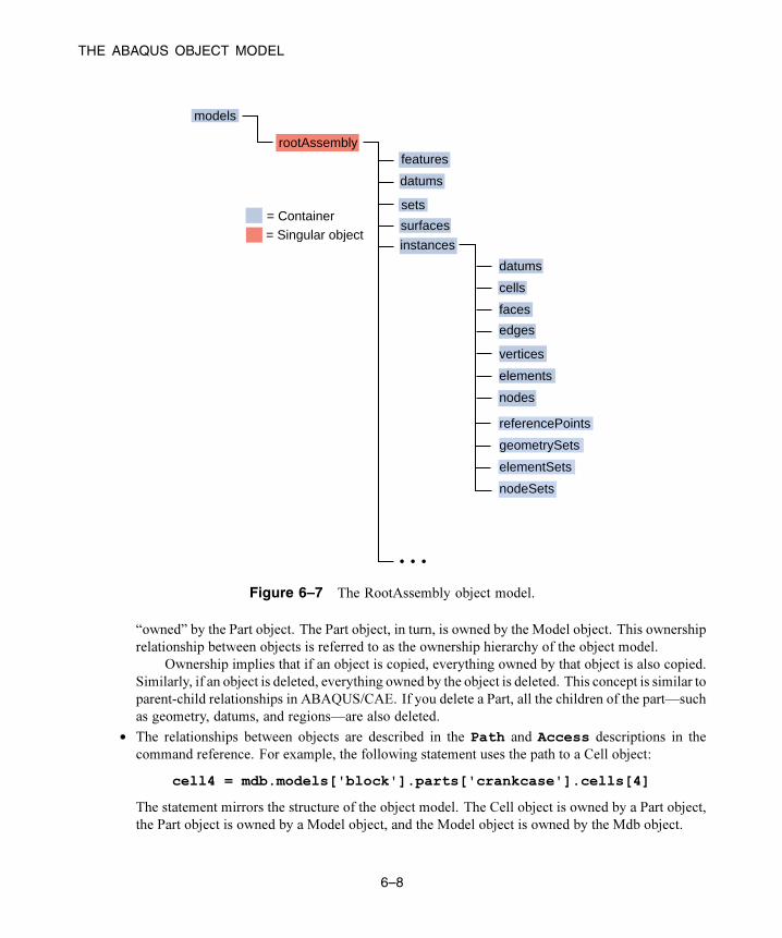
THE ABAQUS OBJECT MODEL
models
features
datums
surfaces
sets
instances
datums
cells
faces
edges
vertices
elements
nodes
= Container = Singular object
rootAssembly
referencePoints
geometrySets
elementSets
nodeSets
Figure 6–7 The RootAssembly object model.
“owned” by the Part object. The Part object, in turn, is owned by the Model object. This ownership
relationship between objects is referred to as the ownership hierarchy of the object model.
Ownership implies that if an object is copied, everything owned by that object is also copied.
Similarly, if an object is deleted, everything owned by the object is deleted. This concept is similar to
parent-child relationships in ABAQUS/CAE. If you delete a Part, all the children of the part—such
as geometry, datums, and regions—are also deleted.
• The relationships between objects are described in the Path and Access descriptions in the
command reference. For example, the following statement uses the path to a Cell object:
cell4 = mdb.models['block'].parts['crankcase'].cells[4]
The statement mirrors the structure of the object model. The Cell object is owned by a Part object,
the Part object is owned by a Model object, and the Model object is owned by the Mdb object.
6–8

THE ABAQUS OBJECT MODEL
• The associations between the objects are captured by the object model. Objects can refer to other
objects; for example, the section objects refer to a material, and the interaction objects refer to a
region, to steps, and possibly to amplitudes. An object that refers to another object usually has a
data member that indicates the name of the object to which it is referring. For example, material is
a member of the section objects, and createStepName is a member of the interaction objects.
6.1.5 Abstract base type
The ABAQUS object model includes the concept of an abstract base type. An abstract base type allows
similar objects to share common attributes. For example, pressure and concentrated force are both
kinds of loads. Object-oriented programmers call the relationship between pressure and load an “is a”
relationship—a pressure is a kind of load. In this example “Load” is the name of the abstract base type.
In the type hierachy Pressure and ConcentratedForce types have a base type Load. A Pressure “is a”
Load.
In Figure 6–8 AnalysisStep and Step are both abstract base types. In terms of the real world a static
step is an analysis step and a static step is also a step. In terms of the object model a StaticStep object is
an AnalysisStep object and a StaticStep object is also a Step object.
Step
InitialStep AnalysisStep
StaticStep BuckleStep
Figure 6–8 An example of the “is a” relationships between objects.
In contrast the object model figures described at the beginning of this section show what object-oriented
programmers call “has a” relationships between objects. For example, a session has a viewport
repository, and a model has a root assembly.
ABAQUS uses the name of the abstract base type as the name of the repository that contains
objects of similar types. For example, the StaticStep, BuckleStep, and FrequencyStepconstructors all create objects in the steps repository. Other abstract base types include Amplitude,
BoundaryCondition, Datum, Field, Interaction, and Section.
The term “abstract” implies that the ABAQUS object model does not contain an object that has the
type of an abstract base type. For example, there are no objects of type Load or Step in the ABAQUS
object model. In contrast, the Feature object is a base type, but it is not abstract. The ABAQUS object
model includes Feature objects.
6–9

THE ABAQUS OBJECT MODEL
6.1.6 Importing modules to extend the object model
To access the objects referred to by the Model object, such as Part and Section objects, ABAQUS/CAE
extends or augments the object model by importing additional modules. For example, to create or access
a Part object, ABAQUS/CAE needs to import the partmodule. ABAQUS/CAE imports all the modules
when you start a session. As a result the entire object model is available to your scripts.
However, in some cases, your script may need to import a module; for example, to access a module
constant, type, or function. In addition, it is useful for you to know which module ABAQUS/CAE
imported to augment the object model with a particular object. You have already seen the syntax to
import a module:
import partimport section
In general, you should use the following approach to importing ABAQUS modules:
import modulename
The description of an object in the ABAQUS Scripting Reference Manual includes an Accesssection that describes which module ABAQUS/CAE imported to make the object available and how
you can access the object from a command. After ABAQUS/CAE imports a module, all the objects
associated with the module become available to you. In addition, all the methods andmembers associated
with each object are also available.
The following table describes the relationship between some of the modules in the ABAQUS
Scripting Interface and the functionality of the modules and toolsets found in ABAQUS/CAE:
Module ABAQUS/CAE functionality
assembly The Assembly module
datum The Datum toolset
interaction The Interaction module
job The Job module
load The Load module
material Materials in the Property module
mesh The Mesh module
part The Part module
partition The Partition toolset
section Sections in the Property module
sketch The Sketch module
6–10
COPYING AND DELETING ABAQUS SCRIPTING INTERFACE OBJECTS
step The Step module
visualization The Visualization module
xyPlot The X–Y toolset
6.2 Copying and deleting ABAQUS Scripting Interface objects
The following section describes how you copy and delete ABAQUS Scripting Interface objects. The
following topics are covered:
• “Creating a copy of an object,” Section 6.2.1
• “More on copying objects,” Section 6.2.2
• “Deleting objects,” Section 6.2.3
6.2.1 Creating a copy of an object
Most ABAQUS objects have a method that creates a copy of the object. The same command provides the
name of the new object. Methods that create a copy of an object are called copy constructors. Although
copy constructors exist for most objects, in most cases they are not documented in the ABAQUSScripting
Reference Manual. The format of a copy constructor is
ObjectName(name='name', objectToCopy=objectToBeCopied)
A copy constructor returns an object of the type of objectToBeCopiedwith the given name. For example,
the following statements show you can create a Part object and then use a copy constructor to create a
second Part object that is a copy of the first:
firstBolt = mdb.models['Metric'].Part(name='boltPattern', dimensionality=THREE_D,type=DEFORMABLE_BODY)
secondBolt = mdb.models['Metric'].Part(name='newBoltPattern', objectToCopy=firstBolt)
You can also use the copy constructor to create a new object in a different model.
firstBolt = mdb.models['Metric'].Part(name='boltPattern', dimensionality=THREE_D,type=DEFORMABLE_BODY)
secondBolt = mdb.models['SAE'].Part(name='boltPattern', objectToCopy=firstBolt)
6–11

COPYING AND DELETING ABAQUS SCRIPTING INTERFACE OBJECTS
6.2.2 More on copying objects
To create a copy of an object, some objects use the base type described in “Abstract base type,”
Section 6.1.5. For example, to copy a HomogeneousSolidSection object, you use the abstract base type
Section constructor.
import materialimport sectionimpactModel = mdb.Model(name='Model A')mySteel = impactModel.Material(name='Steel')
# Create a section
firstSection = impactModel.HomogeneousSolidSection(name='steelSection 1', material='Steel',thickness=1.0)
# Copy the section
secondSection = impactModel.Section(name='steelSection 2', section=firstSection)
6.2.3 Deleting objects
In general, if you can create an object, you can delete the object. For example, the following statements
create a Material object in the material repository:
myMaterial = mdb.models['Model-1'].Material(name='aluminum')
You can use the Python del statement to delete an object, but you must provide the full path to the
object.
del mdb.models['Model-1'].materials['aluminum']
The variable myMaterial that referred to the object still exists; however, the variable no longer refers
to the object. You can use the del statement to delete the variable.
del myMaterial
Conversely, if you create the object as before but delete the variable that referred to the object, only
the variable is deleted; the object still exists. You can assign a new variable to the object.
myMaterial = mdb.models['Model-1'].Material(name='aluminum')del myMaterial
6–12

ABAQUS/CAE SEQUENCES
myNewMaterial = mdb.models['Model-1'].materials['aluminum']
The previous explanation does not apply to the few ABAQUS/CAE objects that are not members
of either an Mdb object or a Session object; for example, XYData and Leaf objects. These objects are
sometimes referred to as “temporary,” and the delete semantics for these objects are the same as for
standard Python objects. The object exists as long as there is a reference to it. If you delete the reference,
the object is also deleted.
6.3 ABAQUS/CAE sequences
Some methods take arguments that are described as “a sequence of sequences of Floats” or “a sequence
of sequences of Ints.” Data that are entered into the table editor in ABAQUS/CAE appear as a sequence
of sequences in the equivalent ABAQUS Scripting Interface command. In effect the data are a two-
dimensional array. The data across one row form one sequence, and multiple rows form a sequence
of those sequences. For example, consider the case where the user is creating an elastic material and
describing a temperature-dependent behavior.
The equivalent ABAQUS Scripting Interface command is
mdb.models['Model-1'].materials['steel'].Elastic(temperatureDependency=TRUE, table=((200.0E9, 0.3, 0.0),(210.0E9, 0.3, 100.0),(220.0E9, 0.3, 250.0),(225.0E9, 0.3, 500.0)))
The table argument is described in the ABAQUS Scripting ReferenceManual as a sequence of sequences
of Floats.
Lists, tuples, strings, and arrays are described in “Sequences,” Section 4.5.4. In addition, the
ABAQUS Scripting Interface defines some of its own sequences that contain objects of the same type.
6–13
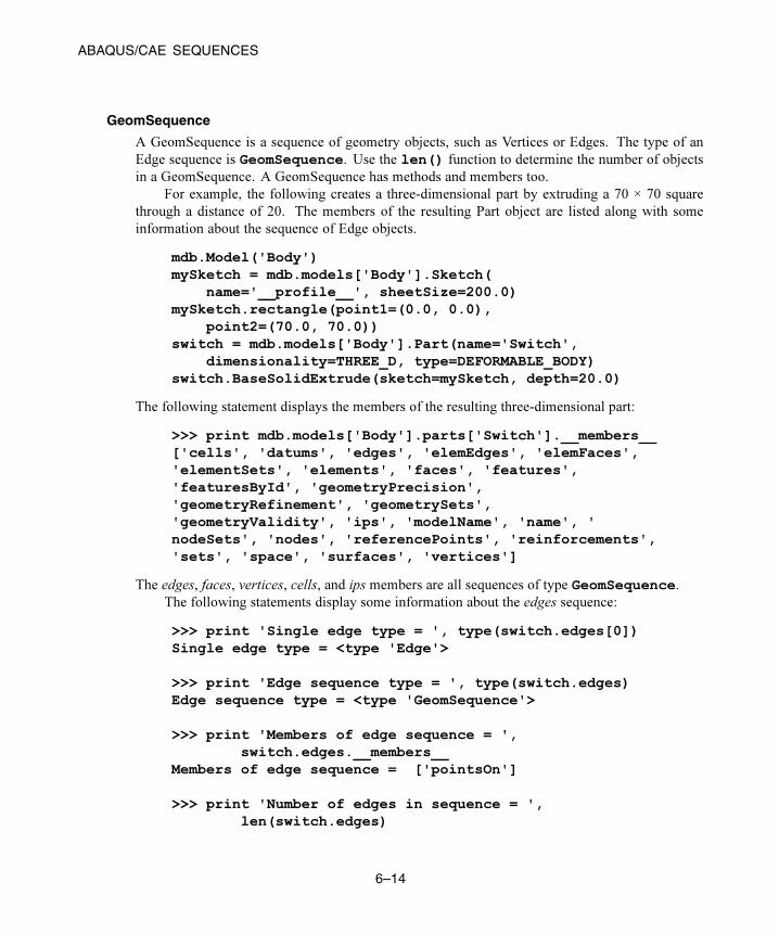
ABAQUS/CAE SEQUENCES
GeomSequence
A GeomSequence is a sequence of geometry objects, such as Vertices or Edges. The type of an
Edge sequence is GeomSequence. Use the len() function to determine the number of objects
in a GeomSequence. A GeomSequence has methods and members too.
For example, the following creates a three-dimensional part by extruding a 70 × 70 square
through a distance of 20. The members of the resulting Part object are listed along with some
information about the sequence of Edge objects.
mdb.Model('Body')mySketch = mdb.models['Body'].Sketch(
name='__profile__', sheetSize=200.0)mySketch.rectangle(point1=(0.0, 0.0),
point2=(70.0, 70.0))switch = mdb.models['Body'].Part(name='Switch',
dimensionality=THREE_D, type=DEFORMABLE_BODY)switch.BaseSolidExtrude(sketch=mySketch, depth=20.0)
The following statement displays the members of the resulting three-dimensional part:
>>> print mdb.models['Body'].parts['Switch'].__members__['cells', 'datums', 'edges', 'elemEdges', 'elemFaces','elementSets', 'elements', 'faces', 'features','featuresById', 'geometryPrecision','geometryRefinement', 'geometrySets','geometryValidity', 'ips', 'modelName', 'name', 'nodeSets', 'nodes', 'referencePoints', 'reinforcements','sets', 'space', 'surfaces', 'vertices']
The edges, faces, vertices, cells, and ips members are all sequences of type GeomSequence.The following statements display some information about the edges sequence:
>>> print 'Single edge type = ', type(switch.edges[0])Single edge type = <type 'Edge'>
>>> print 'Edge sequence type = ', type(switch.edges)Edge sequence type = <type 'GeomSequence'>
>>> print 'Members of edge sequence = ',switch.edges.__members__
Members of edge sequence = ['pointsOn']
>>> print 'Number of edges in sequence = ',len(switch.edges)
6–14

NAMESPACE
Number of edges in sequence = 12
MeshSequence
A sequence of Nodes or Elements.
SurfSequence
A sequence of Surfaces.
6.4 Namespace
Namespace is an important concept for the ABAQUS Scripting Interface programmer. A namespace
can be thought of as a program execution environment, and namespaces are independent of each other.
Namespaces prevent conflict between variable names. You can use the same variable name to refer
to different objects in different name spaces. Figure 6–9 illustrates how commands interact with the
ABAQUS/CAE kernel. ABAQUS Scripting Interface commands are issued to the Python interpreter
from either the GUI, the command line interface, or a script. ABAQUS/CAE executes these commands
in one of two namespaces.
Script namespace
ABAQUS Scripting Interface commands issued from scripts and from the command line interface
are executed in the script namespace. Commands issued from File→Run Script are also executed
in the script namespace. For example, if you enter the following statement from the command line
interface to create a viewport:
myViewport = session.Viewport(name='newViewport',width=100, height=100)
the variable myViewport exists only in the script namespace.
Journal namespace
ABAQUS Scripting Interface commands issued by the GUI are executed in the journal namespace.
For example, if you use the GUI to partition an edge, ABAQUS/CAE writes the following
statements to the replay file, abaqus.rpy:
p1 = mdb.models['Model A'].parts['Part 3D A']e = p1.edgesedges =(e[23], )p1.PartitionEdgeByParam(edges=edges, parameter=0.5)
The variables defined in the replay file (p1, e, and edges, in the above example) exist only in
the journal namespace. ABAQUS/CAE issues an exception if you attempt to refer to one of these
6–15
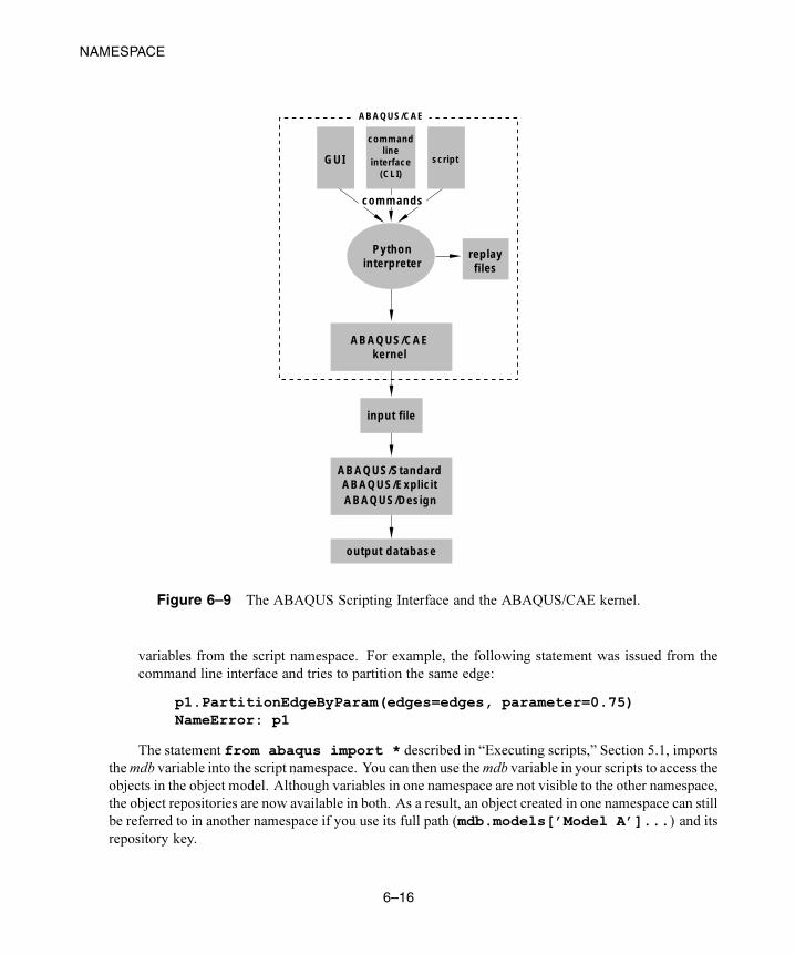
NAMESPACE
GUI
command�line�
interface�(CLI)
script
Python�interpreter
replay�files
ABAQUS/CAE�kernel
commands
input file
ABAQUS/Standard�ABAQUS/Explicit
output database
ABAQUS/CAE
�
�ABAQUS/Design
Figure 6–9 The ABAQUS Scripting Interface and the ABAQUS/CAE kernel.
variables from the script namespace. For example, the following statement was issued from the
command line interface and tries to partition the same edge:
p1.PartitionEdgeByParam(edges=edges, parameter=0.75)NameError: p1
The statement from abaqus import * described in “Executing scripts,” Section 5.1, imports
themdb variable into the script namespace. You can then use themdb variable in your scripts to access the
objects in the object model. Although variables in one namespace are not visible to the other namespace,
the object repositories are now available in both. As a result, an object created in one namespace can still
be referred to in another namespace if you use its full path (mdb.models[’Model A’]...) and itsrepository key.
6–16

SPECIFYING A REGION
For example, although the variable p1 in the above statement cannot be accessed from the script
namespace, you can still use the command line interface to access the part to which p1 referred.
myPart = mdb.models['Model A'].parts['Part 3D A']
The model and part repositories are available in both the journal and script namespaces. You can also
create your own variable p1 from the command line interface or from a script.
p1 = myPart
The variable p1 in the script namespace is independent of the variable p1 in the journal namespace.
6.5 Specifying what is displayed in the viewport
While a script is running and moving between models, modules, parts, and assemblies, you can control
the contents of specified viewports. The contents can be one of the following:
• A part
• The assembly
• A sketch
• Data from an output database
• An X–Y plot
• Empty
In some cases you will want to update the contents of the viewport as the model changes; for example, to
illustrate how the assembly was partitioned prior to meshing. However, frequent updates to a viewport
will slow down your script, and you may want to leave the viewport empty until the script has completed.
Alternatively, you can display an object that the script is not operating on; for example, you can display
a part while the script operates on the assembly.
You use the following command to change the contents of a specified viewport:
session.viewports[name].setvalues(displayedObject=object)
The displayedObject argument can be a Part, Assembly, Sketch, Odb, or XYPlot object or None.If displayedObject=None, ABAQUS/CAE displays an empty viewport. For more information, see
“setValues,” Section 8.2.20 of the ABAQUS Scripting Reference Manual.
6.6 Specifying a region
Many of the commands used by the ABAQUS Scripting Interface require a region argument. For
example,
6–17

SPECIFYING A REGION
• Load commands use the region argument to specify where the load is applied. You apply a
concentrated force to vertices; you apply pressure to a face or an edge.
• Mesh commands, such as setting the element type and creating the mesh, use the region argument
to specify where the operation should be applied.
• Set commands use the region argument to specify the region that comprises the set.
A region can be either a predefined Set or Surface object or a temporary Region object. For more
information, see Chapter 39, “Region commands,” of the ABAQUS Scripting Reference Manual.
You should not rely on the integer id to identify a vertex, edge, face, or cell in a region command;
for example, myFace=myModel.parts[’Door’].faces[3]. The id can change if you add or
delete features to your model; in addition, the id can change with a new release of ABAQUS.
Rather than using the integer id, you should use the findAt method to identify a vertex, edge,
face, or cell. The arguments to findAt are an arbitrary point on an edge, face, or cell or the X-, Y-, and
Z-coordinates of a vertex. findAt returns the id of the vertex or the id of the edge, face, or cell that
includes the arbitrary point.
findAt uses the ACIS tolerance of 1E-6. As a result, findAt returns any entity that is at the
arbitary point specified or at a distance of less than 1E-6 from the arbitary point. The arbitrary point
must not be shared by a second edge, face, or cell. If two entities intersect or coincide at the arbitary
point, findAt chooses the first entity that it encounters; and you should not rely on the return value
being consistent.
Alternatively, if you are working with an existing model that contains named regions, you can
specify a region by referring to its name. For example, in the example described in “Investigating the
skew sensitivity of shell elements,” Section 7.3, you create a model using ABAQUS/CAE. While you
define the model, you must create a set that includes the vertex at the center of a planar part and you must
name the set CENTER. You subsequently run a script that parameterizes the model and performs a series
of analyses. The script uses the named region to retrieve the displacement and the bending moment
at the center of the plate. The following statement refers to the set that you created and named using
ABAQUS/CAE:
centerNSet = odb.rootAssembly.nodeSets['CENTER']
The following script illustrates how you can create a region. Regions are created from each of the
following:
• A sequence of tuples indicating the vertices, edges, faces, or cells in the region. The sequence can
include multiple tuples of the same type.
• A sequence of tuples indicating a combination of the vertices, edges, faces, and cells in the region.
The tuples can appear in any order in the sequence. In addition, you can include multiple tuples of
the same type, and you can omit any type from the sequence.
• A Surface object specifying an entity and the side of the entity.
Use the following command to retrieve the script:
abaqus fetch job=createRegions
6–18

SPECIFYING A REGION
"""createRegions.py
Script to illustrate different techniques for defining regions."""
# Import the modules used by this script.
from abaqus import *from abaqusConstants import *import partimport assemblyimport stepimport loadimport interaction
myModel = mdb.models['Model-1']
# Create a new Viewport for this example.
myViewport=session.Viewport(name='Region syntax',origin=(20, 20), width=200, height=100)
# Create a Sketch and draw two rectangles.
mySketch = myModel.Sketch(name='Sketch A',sheetSize=200.0)
mySketch.rectangle(point1=(-40.0, 30.0),point2=(-10.0, 0.0))
mySketch.rectangle(point1=(10.0, 30.0),point2=(40.0, 0.0))
# Create a 3D part and extrude the rectangles.
door = myModel.Part(name='Door',dimensionality=THREE_D, type=DEFORMABLE_BODY)
door.BaseSolidExtrude(sketch=mySketch, depth=20.0)
6–19

SPECIFYING A REGION
# Instance the part.
myAssembly = myModel.rootAssemblydoorInstance = myAssembly.Instance(name='Door-1',
part=door)
# Select two vertices.
pillarVertices = doorInstance.vertices.findAt(((-40,30,0),), ((40,0,0),) )
# Create a static step.
myModel.StaticStep(name='impact',previous='Initial', initialInc=1, timePeriod=1)
# Create a concentrated force on the selected# vertices.
myPillarLoad = myModel.ConcentratedForce(name='pillarForce', createStepName='impact',region=(pillarVertices,), cf1=12.50E4)
# Select two faces
topFace = doorInstance.faces.findAt(((-25,30,10),))bottomFace = doorInstance.faces.findAt(((-25,0,10),))
# Create a pressure load on the selected faces.# You can use the "+" notation if the entities are of# the same type and are from the same part instance.
myFenderLoad = myModel.Pressure(name='pillarPressure', createStepName='impact',region=((topFace+bottomFace, SIDE1),),magnitude=10E4)
# Select two edges from one instance.
myEdge1 = doorInstance.edges.findAt(((10,15,20),))
6–20

SPECIFYING A REGION
myEdge2 = doorInstance.edges.findAt(((10,15,0),))
# Create a boundary condition on one face,# two edges, and two vertices.
myDisplacementBc= myModel.DisplacementBC(name='xBC', createStepName='impact',region=(pillarVertices, myEdge1+myEdge2,topFace), u1=5.0)
# Select two faces using an arbitrary point# on the face.
faceRegion = doorInstance.faces.findAt(((-30,15,20), ), ((30,15,20),))
# Create a surface containing the two faces.# Indicate which side of the surface to include.
mySurface = myModel.rootAssembly.Surface(name='exterior', side1Faces=faceRegion)
# Create an elastic foundation using the surface.
myFoundation = myModel.ElasticFoundation(name='elasticFloor', createStepName='Initial',surface=mySurface, stiffness=1500)
# Display the assembly along with the new boundary# conditions and loads.
myViewport.setValues(displayedObject=myAssembly)myViewport.assemblyDisplay.setValues(step='impact',
loads=ON, bcs=ON, fields=ON)
6–21

PROMPTING THE USER FOR INPUT
6.7 Prompting the user for input
You may want to request input from a user while an ABAQUS Scripting Interface script is executing.
There are many reasons for requesting input; for example, to specify design parameters, to enable a macro
to take action based on the input received, or to force parts of the script to be repeated. The ABAQUS
Scripting Interface provides three functions that request input from the user and return the data entered
by the user.
• The getInput function requests a single input from the user from a text field in a dialog box. For
more information, see “Requesting a single input from the user,” Section 6.7.1.
• The getInputs function requests multiple inputs from the user from text fields in a dialog box.
For more information, see “Requesting multiple inputs from the user,” Section 6.7.2.
• The getWarningReply function requests a reply to a warning message from the user from
a warning dialog box. For more information, see “Requesting a warning reply from the user,”
Section 6.7.3.
Note: You cannot use a script that contains getInput, getInputs or getWarningReply if you
are running the script from the command line and passing the script name to the command line options
-start,-replay or -noGUI.
6.7.1 Requesting a single input from the user
The getInput function displays a dialog box in the center of the main window, and the user enters
the requested value in the text field in the dialog box. The value is returned to the executing script as a
String after the user presses the [Enter] key or clicksOK. Optionally, you can specify a default value to be
displayed in the text field. The getInput function does not provide any error checking; it is the script
author’s responsibility to verify the user input. For more information, see “getInput,” Section 47.5.1 of
the ABAQUS Scripting Reference Manual.
The following examples illustrate the use of the getInput function. The first example shows a
script that uses the getInput function to obtain a number from the user. The script then prints the
square root of that number.
from abaqus import getInputfrom math import sqrtnumber = float(getInput('Enter a number:'))print sqrt(number)
The float function on the third line converts the string returned by getInput into a floating point
number. The following figure shows the dialog box that appears when this script is executed:
6–22
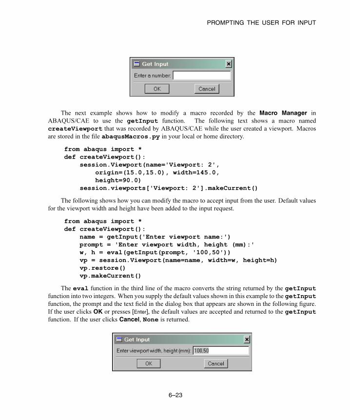
PROMPTING THE USER FOR INPUT
The next example shows how to modify a macro recorded by the Macro Manager in
ABAQUS/CAE to use the getInput function. The following text shows a macro named
createViewport that was recorded by ABAQUS/CAE while the user created a viewport. Macros
are stored in the file abaqusMacros.py in your local or home directory.
from abaqus import *def createViewport():
session.Viewport(name='Viewport: 2',origin=(15.0,15.0), width=145.0,height=90.0)
session.viewports['Viewport: 2'].makeCurrent()
The following shows how you can modify the macro to accept input from the user. Default values
for the viewport width and height have been added to the input request.
from abaqus import *def createViewport():
name = getInput('Enter viewport name:')prompt = 'Enter viewport width, height (mm):'w, h = eval(getInput(prompt, '100,50'))vp = session.Viewport(name=name, width=w, height=h)vp.restore()vp.makeCurrent()
The eval function in the third line of the macro converts the string returned by the getInputfunction into two integers. When you supply the default values shown in this example to the getInputfunction, the prompt and the text field in the dialog box that appears are shown in the following figure.
If the user clicks OK or presses [Enter], the default values are accepted and returned to the getInputfunction. If the user clicks Cancel, None is returned.
6–23
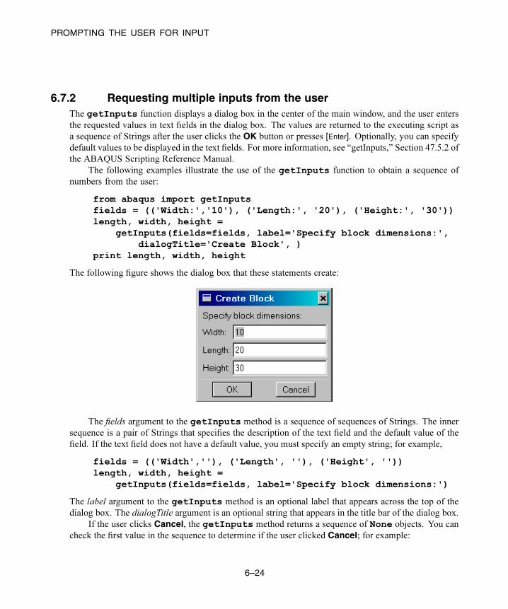
PROMPTING THE USER FOR INPUT
6.7.2 Requesting multiple inputs from the user
The getInputs function displays a dialog box in the center of the main window, and the user enters
the requested values in text fields in the dialog box. The values are returned to the executing script as
a sequence of Strings after the user clicks the OK button or presses [Enter]. Optionally, you can specify
default values to be displayed in the text fields. For more information, see “getInputs,” Section 47.5.2 of
the ABAQUS Scripting Reference Manual.
The following examples illustrate the use of the getInputs function to obtain a sequence of
numbers from the user:
from abaqus import getInputsfields = (('Width:','10'), ('Length:', '20'), ('Height:', '30'))length, width, height =
getInputs(fields=fields, label='Specify block dimensions:',dialogTitle='Create Block', )
print length, width, height
The following figure shows the dialog box that these statements create:
The fields argument to the getInputs method is a sequence of sequences of Strings. The inner
sequence is a pair of Strings that specifies the description of the text field and the default value of the
field. If the text field does not have a default value, you must specify an empty string; for example,
fields = (('Width',''), ('Length', ''), ('Height', ''))length, width, height =
getInputs(fields=fields, label='Specify block dimensions:')
The label argument to the getInputs method is an optional label that appears across the top of the
dialog box. The dialogTitle argument is an optional string that appears in the title bar of the dialog box.
If the user clicks Cancel, the getInputs method returns a sequence of None objects. You can
check the first value in the sequence to determine if the user clicked Cancel; for example:
6–24

INTERACTING WITH ABAQUS/Standard AND ABAQUS/Explicit
fields = (('Density',''), ('Youngs modulus', ''))density, modulus = getInputs(fields, 'Material properties')if density == None:
print 'User pressed Cancel'
6.7.3 Requesting a warning reply from the user
The getWarningReply function displays a warning dialog box in the center of the main window,
and the user clicks on one of the standard reply buttons in the dialog box. The clicked button value is
returned to the executing script. For more information, see “getWarningReply,” Section 47.5.3 of the
ABAQUS Scripting Reference Manual.
The following example illustrates the use of the getWarningReply function:
from abaqus import getWarningReply, YES, NO
reply = getWarningReply(message='Okay to continue?', buttons=(YES,NO))if reply == YES:
print 'YES clicked'elif reply == NO:
print 'NO clicked'
The following figure shows the dialog box that appears when this script is executed:
6.8 Interacting with ABAQUS/Standard and ABAQUS/Explicit
The Job commands include methods that allow you to submit jobs to ABAQUS/Standard and
ABAQUS/Explicit. This section describes how you can interact with ABAQUS/Standard and
ABAQUS/Explicit and synchronize your scripts with the analysis job. The following topics are covered:
• “Processing messages from ABAQUS/Standard and ABAQUS/Explicit,” Section 6.8.1
• “Waiting for a job to complete,” Section 6.8.2
• “An example of a callback function,” Section 6.8.3
6–25

INTERACTING WITH ABAQUS/Standard AND ABAQUS/Explicit
6.8.1 Processing messages from ABAQUS/Standard and
ABAQUS/Explicit
You can use the addMessageCallback method to associate an event-driven function with
a particular message that is retrieved from ABAQUS/Standard or ABAQUS/Explicit. When
ABAQUS/CAE retrieves the specific message from ABAQUS/Standard or ABAQUS/Explicit, the
function executes and takes the necessary action. This type of function is called a callback function.
The addMessageCallback method specifies which callback function to use for which message.
The arguments to addMessageCallback are:
• The name of the job to monitor for messages.
• The message from ABAQUS/Standard or ABAQUS/Explicit that causes the callback function to
execute.
• The name of the callback function.
• An object to pass to the callback function.
These arguments allow you to associate the callback function with both a particular job and a particular
message. Alternatively, you can associate the callback function with all jobs and all messages. The
commands are described in Chapter 28, “Messaging commands,” of the ABAQUS Scripting Reference
Manual.
The interface definition of the callback function is
def functionName(jobName, messageType, data, userData)
The arguments to the callback function are:
• jobName: A String specifying the name of the job to be monitored. You can also use the
SymbolicConstant ANY_JOB that specifies that the callback function will monitor messages from
all jobs.
• messageType: A SymbolicConstant specifying the message type that will call the callback
function. You can also use the SymbolicConstant ANY_MESSAGE_TYPE that specifies that all
messages will call the callback function. The following is a list of the message types issued by
ABAQUS/Standard and ABAQUS/Explicit:
– ABORTED
– ANY_JOB
– ANY_MESSAGE_TYPE
– COMPLETED
– END_STEP
– ERROR
– HEADING
– HEALER_JOB
6–26

INTERACTING WITH ABAQUS/Standard AND ABAQUS/Explicit
– HEALER_TYPE
– INTERRUPTED
– ITERATION
– JOB_ABORTED
– JOB_COMPLETED
– JOB_INTERRUPTED
– JOB_SUBMITTED
– MONITOR_DATA
– ODB_FILE
– ODB_FRAME
– SIMULATION_ABORTED
– SIMULATION_COMPLETED
– SIMULATION_INTERRUPTED
– SIMULATION_SUBMITTED
– STARTED
– STATUS
– STEP
– WARNING
• data: A DataObject object containing the message data. The following list describes the members
of the DataObject object:
– clientHost: A String specifying the host name of the machine that is running the analysis.
– clientName: A String specifying the name of the client that sent the message. Possible values
are
– “BatchPre” (the input file preprocessor)
– “Packager” (the ABAQUS/Explicit preprocessor packager)
– “Standard” (the ABAQUS/Standard analysis)
– “Explicit” (the ABAQUS/Explicit analysis)
– “Calculator” (the postprocessing calculator)
– phase: A SymbolicConstant specifying the phase of the analysis. Possible values are
• BATCHPRE_PHASE
• PACKAGER_PHASE
• STANDARD_PHASE
• EXPLICIT_PHASE
• CALCULATOR_PHASE
• HEALER_PHASE
6–27

INTERACTING WITH ABAQUS/Standard AND ABAQUS/Explicit
– processId: An Int specifying the process ID of the analysis program.
– threadId: An Int specifying the thread ID of the analysis program. Threads are used for parallel
or multiprocessing; in most cases threadId is set to zero.
– timeStamp: An Int specifying the time the message was sent in seconds since 00:00:00 UTC,
January 1, 1970.
• userData: Any Python object or None. This object is passed as the userData argument to
addMessageCallback.
The following script is an example of how you can use the messaging capability of the
ABAQUS Scripting Interface. The callback function will intercept all jobs from all messages from
ABAQUS/Standard or ABAQUS/Explicit and print the messages in the ABAQUS/CAE command line
interface. Use the following command to retrieve the example script:
abaqus fetch job=simpleMonitor
To execute the script, do the following:
• From the ABAQUS/CAE command line interface type from simpleMonitor importprintMessages
• Submit an analysis job as usual.
• To start printing the messages, type printMessages(ON) from the ABAQUS/CAE command
line interface.
• To stop printing the messages, type printMessages(OFF) from the ABAQUS/CAE command
line interface.
"""simpleMonitor.py
Print all messages issued during an ABAQUSanalysis to the ABAQUS/CAE command line interface"""
from abaqus import *from abaqusConstants import *from jobMessage import ANY_JOB, ANY_MESSAGE_TYPE
#~~~~~~~~~~~~~~~~~~~~~~~~~~~~~~~~~~~~~~~~~~~~~~~~~~~~~~~~~def simpleCB(jobName, messageType, data, userData):
"""This callback prints out all themembers of the data objects"""
6–28

INTERACTING WITH ABAQUS/Standard AND ABAQUS/Explicit
format = '%-18s %-18s %s'
print 'Message type: %s'%(messageType)printprint 'data members:'print format%('member', 'type', 'value')
members = dir(data)for member in members:
memberValue = getattr(data, member)memberType = type(memberValue).__name__print format%(member, memberType, memberValue)
#~~~~~~~~~~~~~~~~~~~~~~~~~~~~~~~~~~~~~~~~~~~~~~~~~~~~~~~~~def printMessages(start=ON):
"""Switch message printing ON or OFF"""
if start:monitorManager.addMessageCallback(ANY_JOB,
ANY_MESSAGE_TYPE, simpleCB, None)else:
monitorManager.removeMessageCallback(ANY_JOB,ANY_MESSAGE_TYPE, simpleCB, None)
6.8.2 Waiting for a job to complete
You can use the Job object’s waitForCompletion method to synchronize your script with a job that
has been submitted. If you call the waitForCompletion method after you submit a job, the script
waits until the analysis is complete before continuing. When the script continues, you should check the
status of the job to ensure that the job completed successfully and did not abort. For example, the script
described in “Reproducing the cantilever beam tutorial,” Section 7.1, uses waitForCompletion to
ensure that the analysis job has finished executing successfully before the script opens the resulting output
database and displays a contour plot of the results.
You can use an optional timeOut argument with the waitForCompletionmethod. The timeOut
argument specifies the time in seconds that the script should wait for the job to complete until the script
continues. If the job has not completed before the interval specified by the timeOut argument, the
waitForCompletion method throws an AbaqusException exception. You must include a trystatement to catch the exception thrown by a time out.
6–29

INTERACTING WITH ABAQUS/Standard AND ABAQUS/Explicit
myJob1.submit()try:
myJob1.waitForCompletion(6000)except AbaqusException, message:
print "Job timed out", message
If you do not provide a timeOut argument, the script will wait indefinitely for the job to complete.
In the following example, the script submits myJob1 and waits for it to complete before submitting
myJob2.
myJob1 = mdb.Job(name='Job-1')myJob2 = mdb.Job(name='Job-2')myJob1.submit()myJob1.waitForCompletion()myJob2.submit()myJob2.waitForCompletion()
If you submit more than one job and then issue a waitForCompletion statement, ABAQUS waits
until the job associated with the waitForCompletion statement is complete before checking the
status of the second job. If the second job has already completed, the waitForCompletion method
returns immediately. In the following example the script will not check the status of myJob2 until
myJob1 has completed.
myJob1 = mdb.Job(name='Job-1')myJob2 = mdb.Job(name='Job-2')myJob1.submit()myJob2.submit()myJob1.waitForCompletion()myJob2.waitForCompletion()
If the job submission is delayed using either the at or wait arguments, the interval specified by the
timeOut argument includes both the time required to wait and the time required to execute. It is possible
for the waitForCompletionmethod to time-out before the job is submitted. If this occurs, the script
continues, and the waitForCompletion method throws an exception to indicate that the job did not
run to completion because of a time-out; however, the computer system will still submit the job. As a
result, if you use the at argument, you should add statements that check the status of the job and proceed
accordingly.
6.8.3 An example of a callback function
The following section describes how you can use a callback function as an alternative to the
waitForCompletion method described in “Waiting for a job to complete,” Section 6.8.2.
The example uses messaging commands to synchronize a script with an ABAQUS/Standard or
6–30

INTERACTING WITH ABAQUS/Standard AND ABAQUS/Explicit
ABAQUS/Explicit analysis. Messaging commands set up a callback function that monitors messages
from ABAQUS/Standard and ABAQUS/Explicit. When the desired message is received, the callback
function executes.
The example uses a callback function that responds to all messages from ABAQUS/Standard and
ABAQUS/Explicit. The function decides what action to take based on the messages received from a job
called Deform. If the message indicates that the analysis job is complete, the function opens the output
database created by the job and displays a default contour plot.
#~~~~~~~~~~~~~~~~~~~~~~~~~~~~~~~~~~~~~~~~~~~~~~~~# Define the callback function
from abaqus import *from abaqusConstants import *
import visualization
def onMessage(jobName, messageType, data, viewport):if ((messageType==ABORTED) or (messageType==ERROR)):
print 'Solver problem; stop execution of callback function'elif (messageType==JOB_COMPLETED):
odb = visualization.openOdb(path=jobName + '.odb')viewport.setValues(displayedObject=odb)viewport.odbDisplay.setPlotMode(plotMode=CONTOUR)
The following statements show how the example script can be modified to use the callback function.
After the first statement is executed, the callback function responds to all messages from the job named
Deform. The final two statements create the job and submit it for analysis; the example script has now
finished executing. When the job is complete, the callback function opens the resulting output database
and displays a contour plot.
...myJobName = 'Deform'monitorManager.addMessageCallback(jobName='myJobName',
messageType=ANY_MESSAGE_TYPE, callback=onMessage,userData=myViewport)
myJob = mdb.Job(name=myJobName, model='Beam',description=jobDescription)
myJob.submit()# End of example script.
6–31

USING ABAQUS SCRIPTING INTERFACE COMMANDS IN YOUR ENVIRONMENT FILE
You can use the removeMessageCallback method at the end of the callback function to
remove it from the system. The arguments to the removeMessageCallback method must be
identical to the arguments to the corresponding addMessageCallback command that set up the
callback function.
6.9 Using ABAQUS Scripting Interface commands in your
environment file
The ABAQUS environment file (abaqus_v6.env) is read by ABAQUS/CAE when you start a
session. The environment file can contain ABAQUS Scripting Interface commands. The following is
an example environment file:
scratch = 'c:/temp'pre_memory = 3000000
def onCaeGraphicsStartup():
# Graphics preferences#session.defaultGraphicsOptions.setValues(
displayLists=OFF, dragMode=AS_IS)
def onCaeStartup():
# Print preferences#session.printOptions.setValues(vpDecorations=OFF,
vpBackground=OFF, rendition=COLOR,printCommand='lpr')
session.psOptions.setValues(date=OFF)
# Job preferences#def setJobPreferences(module, userData):
import jobsession.Queue(name='long', hostName='server',
queueName='large', directory='/tmp')addImportCallback('job', setJobPreferences)
6–32
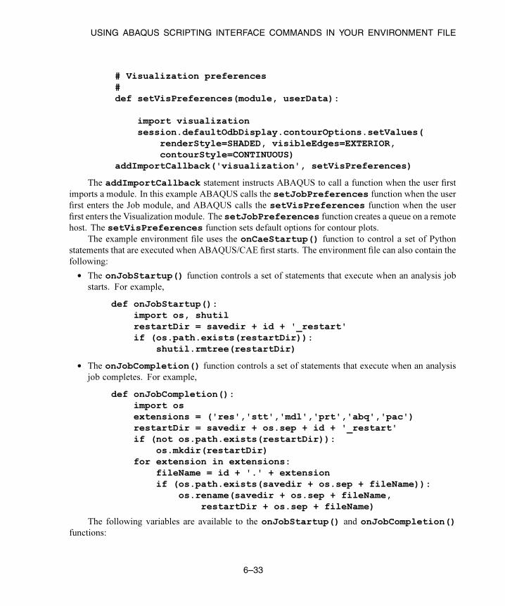
USING ABAQUS SCRIPTING INTERFACE COMMANDS IN YOUR ENVIRONMENT FILE
# Visualization preferences#def setVisPreferences(module, userData):
import visualizationsession.defaultOdbDisplay.contourOptions.setValues(
renderStyle=SHADED, visibleEdges=EXTERIOR,contourStyle=CONTINUOUS)
addImportCallback('visualization', setVisPreferences)
The addImportCallback statement instructs ABAQUS to call a function when the user first
imports a module. In this example ABAQUS calls the setJobPreferences function when the user
first enters the Job module, and ABAQUS calls the setVisPreferences function when the user
first enters the Visualization module. The setJobPreferences function creates a queue on a remote
host. The setVisPreferences function sets default options for contour plots.
The example environment file uses the onCaeStartup() function to control a set of Python
statements that are executed when ABAQUS/CAE first starts. The environment file can also contain the
following:
• The onJobStartup() function controls a set of statements that execute when an analysis job
starts. For example,
def onJobStartup():import os, shutilrestartDir = savedir + id + '_restart'if (os.path.exists(restartDir)):
shutil.rmtree(restartDir)
• The onJobCompletion() function controls a set of statements that execute when an analysis
job completes. For example,
def onJobCompletion():import osextensions = ('res','stt','mdl','prt','abq','pac')restartDir = savedir + os.sep + id + '_restart'if (not os.path.exists(restartDir)):
os.mkdir(restartDir)for extension in extensions:
fileName = id + '.' + extensionif (os.path.exists(savedir + os.sep + fileName)):
os.rename(savedir + os.sep + fileName,restartDir + os.sep + fileName)
The following variables are available to the onJobStartup() and onJobCompletion()functions:
6–33

USING ABAQUS SCRIPTING INTERFACE COMMANDS IN YOUR ENVIRONMENT FILE
id
The job identifier that was specified as the value of the job option from the command line.
savedir
The path to the directory from which the job was submitted.
scrdir
The path to the scratch directory.
analysisType
The type of analysis to be executed. Possible values are STANDARD and EXPLICIT.
For a list of the variables that are available outside of the onJobStartup() and
onJobCompletion() functions, see “Job variables,” Section 4.1.9 of the ABAQUS Installation and
Licensing Guide.
For more information on the environment file, see “Using the ABAQUS environment settings,”
Section 3.4.1 of the ABAQUS Analysis User’s Manual, and Chapter 4, “Customizing the ABAQUS
environment,” of the ABAQUS Installation and Licensing Guide.
6–34

Part III Putting it all together: examples
The section provides examples that illustrate how you can combine ABAQUS Scripting Interface commands
and Python statements to create your own scripts. You can use the scripts to create ABAQUS/CAE models,
submit jobs for analysis, and view the results.
For examples of scripts that read and write from an output database, see “Example scripts that access
data from an output database,” Section 8.10.


REPRODUCING THE CANTILEVER BEAM TUTORIAL
7. ABAQUS Scripting Interface examples
The ABAQUS/CAE example scripts in this chapter illustrate the following:
• How you can use commands from the ABAQUS Scripting Interface to create a simple model, submit
it for analysis, and view the results. “Reproducing the cantilever beam tutorial,” Section 7.1, uses
ABAQUS Scripting Interface commands to reproduce the cantilever beam tutorial described in
Appendix B, “Creating and Analyzing a Simple Model in ABAQUS/CAE,” of Getting Started with
ABAQUS.
• How you can use the ABAQUS Scripting Interface to control the output from the Visualization
module in ABAQUS/CAE (ABAQUS/Viewer).
– “Opening the tutorial output database,” Section 7.2.1, explains how to use abaqus fetch to
retrieve the ABAQUS/CAE tutorial output database.
– “Opening an output database and displaying a contour plot,” Section 7.2.2, explains how to
open the tutorial output database, display a contour plot, and print the resulting viewport to a
file.
– “Printing a contour plot at the end of each step,” Section 7.2.3, explains how to open the tutorial
output database, customize the legend, display a contour plot at the end of each step, and print
the resulting viewports to a file.
• How you can introduce more complex programming techniques into your ABAQUS Scripting
Interface scripts. “Investigating the skew sensitivity of shell elements,” Section 7.3, reproduces the
problem found in “Skew sensitivity of shell elements,” Section 2.3.4 of the ABAQUS Benchmarks
Manual. You use ABAQUS/CAE to create the model, and you use ABAQUS Scripting Interface
commands to parameterize an evaluation of the model by changing its geometry and element type.
The example investigates the sensitivity of the shell elements in ABAQUS to skew distortion when
they are used as thin plates.
The example scripts from this manual can be copied to the user’s working directory by using the
ABAQUS fetch utility:
abaqus fetch job=scriptName
where scriptName.py is the name of the script (see “Execution procedure for ABAQUS/Fetch,”
Section 3.2.12 of the ABAQUS Analysis User’s Manual).
7.1 Reproducing the cantilever beam tutorial
This example uses ABAQUS Scripting Interface commands to reproduce the cantilever beam tutorial
described in Appendix B, “Creating and Analyzing a Simple Model in ABAQUS/CAE,” of Getting
Started with ABAQUS. Figure 7–1 illustrates the model that you will create and analyze.
7–1

REPRODUCING THE CANTILEVER BEAM TUTORIAL
20 mm
25 mm200 mm
0.5 MPa
Figure 7–1 A loaded cantilever beam.
The following topics are covered:
• “Running the example,” Section 7.1.1
• “The cantilever beam example script,” Section 7.1.2
7.1.1 Running the example
Use the following command to retrieve the output database that is read by the scripts:
abaqus fetch job=beamExample
To run the script, do the following:
1. Start ABAQUS/CAE from a directory in which you havewrite permission by typingabaqus cae.
2. From the startup screen, select Run Script.
3. From the Run Script dialog box that appears, enter the path given above and select the file
containing the script.
4. Click OK to run the script.
Note: If ABAQUS/CAE is already running, you can run the script by selecting File→Run Script from
the main menu bar.
7.1.2 The cantilever beam example script
The first line of the script, from abaqus import *, imports the Mdb and Session objects.
The current viewport is session.viewports[’Viewport: 1’], and the current model is
mdb.models[’Model-1’]. Both of these objects are available to the script after you import the
abaqus module. The second line of the script, from abaqusConstants import *, imports
7–2

REPRODUCING THE CANTILEVER BEAM TUTORIAL
the Symbolic Constants defined in the ABAQUS Scripting Interface. The script then creates a new
model that will contain the cantilever beam example and creates a new viewport in which to display the
model and the results of the analysis. For a description of the commands used in this section, see the
appropriate sections in the ABAQUS Scripting Reference Manual.
The script then imports the Partmodule. Most of the sections in this example begin with importing
the appropriate module, which illustrates how a script can import a module at any time to extend or
augment the object model. However, the ABAQUS Scripting Interface has a convention that all the
required modules are imported at the start of a script; and that convention is followed in other example
scripts in this manual.
"""beamExample.py
Reproduce the cantilever beam example from theAppendix of the Getting Started withABAQUS Manual."""
from abaqus import *from abaqusConstants import *
# Create a model.
myModel = mdb.Model(name='Beam')
# Create a new viewport in which to display the model# and the results of the analysis.
myViewport = session.Viewport(name='Cantilever Beam Example',origin=(20, 20), width=150, height=120)
#-----------------------------------------------------
import part
# Create a sketch for the base feature.
mySketch = myModel.Sketch(name='beamProfile',sheetSize=250.)
# Create the rectangle.
7–3

REPRODUCING THE CANTILEVER BEAM TUTORIAL
mySketch.rectangle(point1=(-100,10), point2=(100,-10))
# Create a three-dimensional, deformable part.
myBeam = myModel.Part(name='Beam', dimensionality=THREE_D,type=DEFORMABLE_BODY)
# Create the part's base feature by extruding the sketch# through a distance of 25.0.
myBeam.BaseSolidExtrude(sketch=mySketch, depth=25.0)
#-----------------------------------------------------
import material
# Create a material.
mySteel = myModel.Material(name='Steel')
# Create the elastic properties: youngsModulus is 209.E3# and poissonsRatio is 0.3
elasticProperties = (209.E3, 0.3)mySteel.Elastic(table=(elasticProperties, ) )
#-------------------------------------------------------
import section
# Create the solid section.
mySection = myModel.HomogeneousSolidSection(name='beamSection',material='Steel', thickness=1.0)
# Assign the section to the region. The region refers# to the single cell in this model.
region = (myBeam.cells,)myBeam.SectionAssignment(region=region,
sectionName='beamSection')
7–4
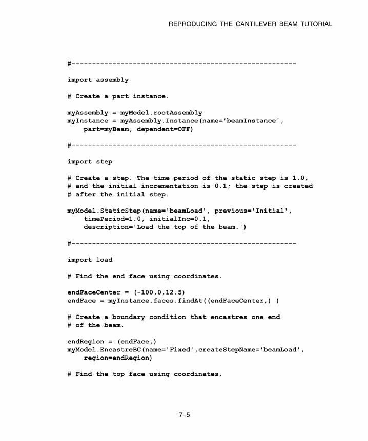
REPRODUCING THE CANTILEVER BEAM TUTORIAL
#-------------------------------------------------------
import assembly
# Create a part instance.
myAssembly = myModel.rootAssemblymyInstance = myAssembly.Instance(name='beamInstance',
part=myBeam, dependent=OFF)
#-------------------------------------------------------
import step
# Create a step. The time period of the static step is 1.0,# and the initial incrementation is 0.1; the step is created# after the initial step.
myModel.StaticStep(name='beamLoad', previous='Initial',timePeriod=1.0, initialInc=0.1,description='Load the top of the beam.')
#-------------------------------------------------------
import load
# Find the end face using coordinates.
endFaceCenter = (-100,0,12.5)endFace = myInstance.faces.findAt((endFaceCenter,) )
# Create a boundary condition that encastres one end# of the beam.
endRegion = (endFace,)myModel.EncastreBC(name='Fixed',createStepName='beamLoad',
region=endRegion)
# Find the top face using coordinates.
7–5

REPRODUCING THE CANTILEVER BEAM TUTORIAL
topFaceCenter = (0,10,12.5)topFace = myInstance.faces.findAt((topFaceCenter,) )
# Create a pressure load on the top face of the beam.
topSurface = ((topFace, SIDE1), )myModel.Pressure(name='Pressure', createStepName='beamLoad',
region=topSurface, magnitude=0.5)
#-------------------------------------------------------
import mesh
# Assign an element type to the part instance.
region = (myInstance.cells,)elemType = mesh.ElemType(elemCode=C3D8I, elemLibrary=STANDARD)myAssembly.setElementType(regions=region, elemTypes=(elemType,))
# Seed the part instance.
myAssembly.seedPartInstance(regions=(myInstance,), size=10.0)
# Mesh the part instance.
myAssembly.generateMesh(regions=(myInstance,))
# Display the meshed beam.
myViewport.assemblyDisplay.setValues(mesh=ON)myViewport.assemblyDisplay.meshOptions.setValues(meshTechnique=ON)myViewport.setValues(displayedObject=myAssembly)
#-------------------------------------------------------
import job
# Create an analysis job for the model and submit it.
jobName = 'beam_tutorial'myJob = mdb.Job(name=jobName, model='Beam',
7–6

GENERATING A CUSTOMIZED PLOT
description='Cantilever beam tutorial')
# Wait for the job to complete.
myJob.submit()myJob.waitForCompletion()
#-------------------------------------------------------
import visualization
# Open the output database and display a# default contour plot.
myOdb = visualization.openOdb(path=jobName + '.odb')myViewport.setValues(displayedObject=myOdb)myViewport.odbDisplay.setPlotMode(CONTOUR)
7.2 Generating a customized plot
The following section provides examples of ABAQUS Scripting Interface scripts that open an output
database and generate a customized plot. In effect, these scripts reproduce the functionality of the
Visualization module in ABAQUS/CAE. The following examples are provided:
• “Opening the tutorial output database,” Section 7.2.1
• “Opening an output database and displaying a contour plot,” Section 7.2.2
• “Printing a contour plot at the end of each step,” Section 7.2.3
7.2.1 Opening the tutorial output database
Each of the following example scripts opens the output database used by the Visualizationmodule tutorial
in Getting Started with ABAQUS. Use the following command to retrieve the output database that is read
by the scripts:
abaqus fetch job=viewer_tutorial
7–7

GENERATING A CUSTOMIZED PLOT
7.2.2 Opening an output database and displaying a contour plot
The following example of a script containing ABAQUS Scripting Interface commands uses the output
database used by Appendix D, “Viewing the Output from Your Analysis,” of Getting Started with
ABAQUS.
Use the following command to retrieve the example script:
abaqus fetch job=viewerOpenOdbAndContour
The script does the following:
• Creates a viewport, and makes it the current viewport.
• Opens an output database.
• Displays a contour plot.
• Displays the model in the first frame of the third step.
• Sets the number of contour intervals and the contour limits.
• Prints a color image of the viewport to a .png file.
"""viewerOpenOdbAndContour.py
Print a contour plot to a local PNG-format file."""
from abaqus import *from abaqusConstants import *import visualization
# Create a new Viewport for this example.
myViewport=session.Viewport(name='Print a contour plot',origin=(10, 10), width=200, height=100)
# Open the output database and associate it# with the new viewport.
odbPath = "viewer_tutorial.odb"myOdb = visualization.openOdb(path=odbPath)
myViewport.setValues(displayedObject=myOdb)
# Display a contour plot of the output database.
7–8

GENERATING A CUSTOMIZED PLOT
myViewport.odbDisplay.setPlotMode(CONTOUR)
# Change to the first frame of the third step.# Remember that indices in Python begin with zero:# The index of the first frame is 0.# The index of the third step is 2.
myViewport.odbDisplay.setFrame(step=2, frame=0)
# Change the number of contour intervals to 10# starting at 0.0 and ending at 0.10.
myViewport.odbDisplay.contourOptions.setValues(numIntervals=10,maxAutoCompute=OFF, maxValue=0.10,minAutoCompute=OFF, minValue=0.0,)
# Generate color output.# Do not print the viewport decorations or the black background.
session.printOptions.setValues(rendition=COLOR,vpDecorations=OFF, vpBackground=OFF)
# Print the viewport to a local PNG-format file.
session.printToFile(fileName='contourPlot', format=PNG,canvasObjects=(myViewport,))
7.2.3 Printing a contour plot at the end of each step
The following example script demonstrates how to produce and print a contour plot at the last frame of
every step within an output database file. The example sets the appropriate contour limits so that all plots
can be viewed within a fixed range.
Use the following command to retrieve the example script:
abaqus fetch job=viewerPrintContours
The script does the following:
7–9
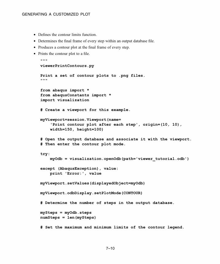
GENERATING A CUSTOMIZED PLOT
• Defines the contour limits function.
• Determines the final frame of every step within an output database file.
• Produces a contour plot at the final frame of every step.
• Prints the contour plot to a file.
"""viewerPrintContours.py
Print a set of contour plots to .png files."""
from abaqus import *from abaqusConstants import *import visualization
# Create a viewport for this example.
myViewport=session.Viewport(name='Print contour plot after each step', origin=(10, 10),width=150, height=100)
# Open the output database and associate it with the viewport.# Then enter the contour plot mode.
try:myOdb = visualization.openOdb(path='viewer_tutorial.odb')
except (AbaqusException), value:print 'Error:', value
myViewport.setValues(displayedObject=myOdb)
myViewport.odbDisplay.setPlotMode(CONTOUR)
# Determine the number of steps in the output database.
mySteps = myOdb.stepsnumSteps = len(mySteps)
# Set the maximum and minimum limits of the contour legend.
7–10

GENERATING A CUSTOMIZED PLOT
myViewport.odbDisplay.contourOptions.setValues(numIntervals=10,maxAutoCompute=OFF, maxValue=0.1,minAutoCompute=OFF, minValue=0.0)
# Establish print preferences.
session.printOptions.setValues(vpBackground=OFF)session.psOptions.setValues(orientation=LANDSCAPE)myViewport.viewportAnnotationOptions.setValues(
triad=OFF,title=OFF,state=OFF)myViewport.odbDisplay.basicOptions.setValues(
coordSystemDisplay=OFF, )
# For each step, obtain the following:# 1) The step key.# 2) The number of frames in the step.# 3) The increment number of the last frame in the step.#
for i in range(numSteps):stepKey = mySteps.keys()[i]step = mySteps[stepKey]numFrames = len(step.frames)
# Go to the last frame.# Display a contour plot.# Display the step description and the increment number.
myViewport.odbDisplay.setFrame(step=i, frame=numFrames-1)myViewport.odbDisplay.setPlotMode(CONTOUR)
# Remove white space from the step key and use the result# to name the file.
fileName=stepKey.replace(' ','')
# Print the viewport to a file.
session.printToFile(fileName, PNG, (myViewport,))
7–11

INVESTIGATING THE SKEW SENSITIVITY OF SHELL ELEMENTS
7.3 Investigating the skew sensitivity of shell elements
In this example you will use ABAQUS/CAE to create the model and store the model in a model database.
The script opens the model database and performs a parametric study on the model. The example
illustrates how you can use a combination of ABAQUS/CAE and the ABAQUS Scripting Interface to
analyze a problem.
This example uses ABAQUS Scripting Interface commands to evaluate the sensitivity of the shell
elements in ABAQUS to skew distortion when they are used as thin plates. Further details can be found in
“Skew sensitivity of shell elements,” Section 2.3.4 of the ABAQUS Benchmarks Manual. The problem
investigates the effects on the accuracy of the bending moment computed at the center of a shell using:
• different shell formulations and
• at different angles.
Figure 7–2 illustrates the basic geometry of the simply supported skew plate with a uniform
distributed load.
1.0 m
x, y, z displacements�constrained on boundary
δx
y
1.0
m
Figure 7–2 A 4 × 4 quadrilateral mesh of the plate.
The plate is loaded by a uniform pressure of 1.0 × 10⁻⁶ MPa applied over the entire surface. The edges of
the plate are all simply supported. The analysis is performed for five different values of the skew angle,
: 90°, 80°, 60°, 40°, and 30°. The analysis is performed for two different quadrilateral elements: S4
and S8R.
The example is divided into two scripts. The controlling script, skewExample.py, imports
skewExampleUtils.py. Use the fetch utility to retrieve the scripts:
abaqus fetch job=skewExampleabaqus fetch job=skewExampleUtils
7–12

INVESTIGATING THE SKEW SENSITIVITY OF SHELL ELEMENTS
The following topics are covered:
• “Creating the model to analyze,” Section 7.3.1
• “Changing the skew angle,” Section 7.3.2
• “Using a script to perform a parametric study,” Section 7.3.3
7.3.1 Creating the model to analyze
You should use ABAQUS/CAE to create your model and to save the resulting model database. You
will then use scripting to parameterize your model, submit an analysis job, and operate on the results
generated.
Start ABAQUS/CAE, and create a model database from the Start Session dialog box. By default,
you are operating on a model named Model-1. The model should include the following:
Part
Create a three-dimensional planar shell part, and name it Plate. Use an approximate size of 5.0.
All sides are 1.0 m long.
Material
Create a material, and name it Steel. The Young’s modulus is 30 MPa, and the Poisson’s ratio is
0.3.
Section
Create a homogeneous shell section that refers to the material called Steel. Name the section
Shell. The plate thickness is 0.01 m. The length/thickness ratio is, thus, 100/1 so that the plate is
thin in the sense that transverse shear deformation should not be significant. Assign the section to
the plate.
Assembly
Create the assembly using a single instance of the part. ABAQUS/CAE names the part instance
Plate-1.
Step
Create a static step and name it Step-1. Enter Apply pressure for the step Description.
Accept the default time period of 1.0 and the default initial increment of 1.0.
Output database requests
Edit the default output database request for field output and select only U, Translations and
rotations, and SF, Section forces and moments, for the whole model after every increment.
Delete all requests for history output.
7–13

INVESTIGATING THE SKEW SENSITIVITY OF SHELL ELEMENTS
Boundary condition
Create a displacement boundary condition, and name it Pinned. The boundary condition pins the
exterior edges of the plate.
Load
Create a pressure load, and name it Pressure. Apply the load to the face of the plate. Accept thedefault side of the plate and use a magnitude of 1.0. This positive pressure will result in a negative
displacement in the 3-direction.
Set
Partition the plate into quarters. Create a set that contains the vertex at the center of the plate, and
name the set CENTER.
Mesh
Create a 4 × 4 swept mesh of quadrilateral elements on the plate.
Keyword editor
You must use the Keyword Editor to request output of section forces and moments for the node
at the center of the plate. When you edited the output database request to select the variable, SF,
ABAQUS/CAE requested output of section forces and moments at element integration points. To
modify this output request, you must add position=NODES to the OUTPUT REQUESTS block
as follows:
*Element Output, position=NODESSF,
Job
Create a job, and name it skew. The job must refer to the model Model-1.
7.3.2 Changing the skew angle
The parameterized script changes the skew angle of the plate and computes the maximum bending
moment at the center for two different element types. The script changes the skew angle by modifying
an angular dimension and selecting the vertices to move. You need to add the angular dimensions and
determine the indices of the dimensions to modify and the vertices to move.
To add the angular dimensions:
1. Return to the Part module.
2. From the main menu bar, select Feature→Edit and select the plate to edit.
3. From the Edit Feature dialog box, select Edit Section Sketch.
7–14
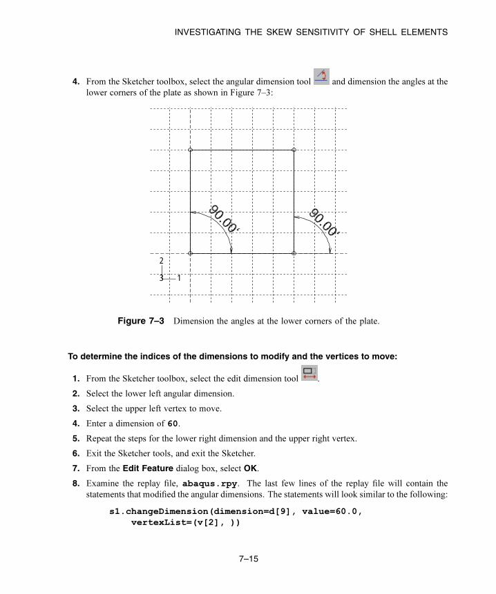
INVESTIGATING THE SKEW SENSITIVITY OF SHELL ELEMENTS
4. From the Sketcher toolbox, select the angular dimension tool and dimension the angles at the
lower corners of the plate as shown in Figure 7–3:
1
2
3
Figure 7–3 Dimension the angles at the lower corners of the plate.
To determine the indices of the dimensions to modify and the vertices to move:
1. From the Sketcher toolbox, select the edit dimension tool .
2. Select the lower left angular dimension.
3. Select the upper left vertex to move.
4. Enter a dimension of 60.
5. Repeat the steps for the lower right dimension and the upper right vertex.
6. Exit the Sketcher tools, and exit the Sketcher.
7. From the Edit Feature dialog box, select OK.
8. Examine the replay file, abaqus.rpy. The last few lines of the replay file will contain the
statements that modified the angular dimensions. The statements will look similar to the following:
s1.changeDimension(dimension=d[9], value=60.0,vertexList=(v[2], ))
7–15

INVESTIGATING THE SKEW SENSITIVITY OF SHELL ELEMENTS
s1.changeDimension(dimension=d[10], value=60.0,vertexList=(v[4], ))
9. The example script, skewExample.py, contains similar statements that modify the angular
dimensions of the plate. The indices of the angular dimensions and vertices in your model must be
the same as the indices in the example script. If the indices are not the same, you must edit the
example script and enter the correct indices.
tmpSketch.changeDimension(dimension=d[9], value=angle,vertexList=(v[2], ))
tmpSketch.changeDimension(dimension=d[10], value=angle,vertexList=(v[4], ))
Save the model database, and name it skew. ABAQUS/CAE saves the model database in a file
called skew.cae. The example script opens this model database and parameterizes the model it
contains.
7.3.3 Using a script to perform a parametric study
The following shows the contents of the script skewExample.py. The parametric study does the
following:
• Opens the model database and creates variables that refer to the part, the assembly, and the part
instance stored in Model-1.
• Creates variables that refer to the four faces and the nine vertices in the instance of the planar shell
part.
• Skews the plate by modifying the angular dimensions in the sketch of the base feature.
• Defines the logical corners of the four faces, and generates a structured mesh.
• Runs the analysis for a range of angles using two element types for each angle.
• Calculates the maximum moment and displacement at the center of the shell.
• Displays X–Y plots in separate viewports of the following:
– Displacement versus skew angle
– Maximum bending moment versus skew angle
– Minimum bending moment versus skew angle
The theoretical results are also plotted.
"""skewExample.py
This script performs a parameter study of element type versusskew angle. For more details, see Problem 2.3.4 in theABAQUS Benchmarks manual.
7–16

INVESTIGATING THE SKEW SENSITIVITY OF SHELL ELEMENTS
Before executing this script you must fetch the appropriatefiles: abaqus fetch job=skewExample
abaqus fetch job=skewExampleUtils.py"""
import partimport meshfrom mesh import S4, S8R, STANDARD, STRUCTUREDimport jobfrom skewExampleUtils import getResults, createXYPlot
# Create a list of angle parameters and a list of# element type parameters.
angles = [90, 80, 60, 40, 30]elemTypeCodes = [S4, S8R]
# Open the model database.openMdb('skew.cae')
model = mdb.models['Model-1']part = model.parts['Plate']feature = part.features['Shell planar-1']assembly = model.rootAssemblyinstance = assembly.instances['Plate-1']job = mdb.jobs['skew']
allFaces = instance.facesregions =(allFaces[0], allFaces[1], allFaces[2], allFaces[3])assembly.setMeshControls(regions=regions,
technique=STRUCTURED)face1 = allFaces.findAt((0.,0.,0.), )face2 = allFaces.findAt((0.,1.,0.), )face3 = allFaces.findAt((1.,1.,0.), )face4 = allFaces.findAt((1.,0.,0.), )allVertices = instance.verticesv1 = allVertices.findAt((0.,0.,0.), )v2 = allVertices.findAt((0.,.5,0.), )v3 = allVertices.findAt((0.,1.,0.), )v4 = allVertices.findAt((.5,1.,0.), )
7–17
INVESTIGATING THE SKEW SENSITIVITY OF SHELL ELEMENTS
v5 = allVertices.findAt((1.,1.,0.), )v6 = allVertices.findAt((1.,.5,0.), )v7 = allVertices.findAt((1.,0.,0.), )v8 = allVertices.findAt((.5,0.,0.), )v9 = allVertices.findAt((.5,.5,0.), )
# Create a copy of the feature sketch to modify.
tmpSketch = model.Sketch('tmp', feature.sketch)v, d = tmpSketch.vertices, tmpSketch.dimensions
# Create some dictionaries to hold results. Seed the# dictionaries with the theoretical results.
dispData, maxMomentData, minMomentData = {}, {}, {}dispData['Theoretical'] = ((90, -.001478), (80, -.001409),
(60, -0.000932), (40, -0.000349), (30, -0.000148))maxMomentData['Theoretical'] = ((90, 0.0479), (80, 0.0486),
(60, 0.0425), (40, 0.0281), (30, 0.0191))minMomentData['Theoretical'] = ((90, 0.0479), (80, 0.0448),
(60, 0.0333), (40, 0.0180), (30, 0.0108))
# Loop over the parameters to perform the parameter study.
for elemCode in elemTypeCodes:
# Convert the element type codes to strings.
elemName = repr(elemCode)dispData[elemName], maxMomentData[elemName], \
minMomentData[elemName] = [], [], []
# Set the element type.
elemType = mesh.ElemType(elemCode=elemCode,elemLibrary=STANDARD)
assembly.setElementType(regions=(instance.faces,),elemTypes=(elemType,))
for angle in angles:
7–18

INVESTIGATING THE SKEW SENSITIVITY OF SHELL ELEMENTS
# Skew the geometry and regenerate the mesh.
tmpSketch.changeDimension(dimension=d[9], value=angle,vertexList=(v[2], ))
tmpSketch.changeDimension(dimension=d[10], value=angle,vertexList=(v[4], ))
feature.setValues(sketch=tmpSketch)part.regenerate()assembly.regenerate()assembly.setLogicalCorners(
region=face1, corners=(v1,v2,v9,v8))assembly.setLogicalCorners(
region=face2, corners=(v2,v3,v4,v9))assembly.setLogicalCorners(
region=face3, corners=(v9,v4,v5,v6))assembly.setLogicalCorners(
region=face4, corners=(v8,v9,v6,v7))assembly.generateMesh(regions=(instance,))
# Run the job, then process the results.
job.submit()job.waitForCompletion()print 'Completed job for %s at %s degrees' % (elemName,
angle)disp, maxMoment, minMoment = getResults()dispData[elemName].append((angle, disp))maxMomentData[elemName].append((angle, maxMoment))minMomentData[elemName].append((angle, minMoment))
# Plot the results.
createXYPlot((10,10), 'Skew 1', 'Displacement - 4x4 Mesh',dispData)
createXYPlot((160,10), 'Skew 2', 'Max Moment - 4x4 Mesh',maxMomentData)
createXYPlot((310,10), 'Skew 3', 'Min Moment - 4x4 Mesh',minMomentData)
The script imports two functions from skewExampleUtils. The functions do the following:
7–19

INVESTIGATING THE SKEW SENSITIVITY OF SHELL ELEMENTS
• Retrieve the displacement and calculate the maximum bending moment at the center of the plate.
• Display curves of theoretical and computed results in a new viewport.
"""skewExampleUtils.py
Utilities for the scripting tutorial Skew Example."""
from abaqus import *import visualizationfrom miscUtils import sorted
#~~~~~~~~~~~~~~~~~~~~~~~~~~~~~~~~~~~~~~~~~~~~~~~~~~~~~~~~~~~~def getResults():
"""Retrieve the displacement and calculate the minimumand maximum bending moment at the center of plate."""
from visualization import ELEMENT_NODAL
# Open the output database.
odb = visualization.openOdb('skew.odb')centerNSet = odb.rootAssembly.nodeSets['CENTER']frame = odb.steps['Step-1'].frames[-1]
# Retrieve Z-displacement at the center of the plate.
dispField = frame.fieldOutputs['U']dispSubField = dispField.getSubset(region=centerNSet)disp = dispSubField.values[0].data[2]
# Average the contribution from each element to the moment,# then calculate the minimum and maximum bending moment at# the center of the plate using Mohr's circle.
momentField = frame.fieldOutputs['SM']momentSubField = momentField.getSubset(region=centerNSet,
position=ELEMENT_NODAL)
7–20

INVESTIGATING THE SKEW SENSITIVITY OF SHELL ELEMENTS
m1, m2, m3 = 0, 0, 0for value in momentSubField.values:
m1 = m1 + value.data[0]m2 = m2 + value.data[1]m3 = m3 + value.data[2]
numElements = len(momentSubField.values)m1 = m1 / numElementsm2 = m2 / numElementsm3 = m3 / numElementsmomentA = 0.5 * (abs(m1) + abs(m2))momentB = sqrt(0.25 * (m1 - m2)**2 + m3**2)maxMoment = momentA + momentBminMoment = momentA - momentB
odb.close()
return disp, maxMoment, minMoment
#~~~~~~~~~~~~~~~~~~~~~~~~~~~~~~~~~~~~~~~~~~~~~~~~~~~~~~~~~~~def createXYPlot(vpOrigin, vpName, plotName, data):
"""Display curves of theoretical and computed results ina new viewport."""
from visualization import USER_DEFINED
vp = session.Viewport(name=vpName, origin=vpOrigin,width=150, height=100)
xyPlot = session.XYPlot(plotName)for elemName, xyValues in sorted(data.items()):
xyData = visualization.XYData(elemName, xyValues)xyPlot.Curve(elemName, xyData)
xyPlot.setValues(curvesToPlot=sorted(data.keys()),xAxisTitle='Skew Angle', xAxisTitleSource=USER_DEFINED,yAxisTitle=plotName, yAxisTitleSource=USER_DEFINED)
vp.setValues(displayedObject=xyPlot)
7–21


Part IV Accessing an output database
This section describes how you access the data in an output database using either the ABAQUS Scripting
Interface or the C++ Application Programming Interface (API). You can read model data and field and history
data from an output database. You can also write field and history data to an output database.
The ABAQUS Scripting Interface commands that read and write data from an output database are
described in Chapter 30, “Odb commands,” of the ABAQUS Scripting Reference Manual.
The C++ commands that read and write data from an output database are described in Chapter 52, “Odb
commands,” of the ABAQUS Scripting Reference Manual.


HOW THE OBJECT MODEL FOR THE OUTPUT DATABASE RELATES TO COMMANDS
8. Using the ABAQUS Scripting Interface to access an
output database
The following sections describe the architecture of an output database and how to use the ABAQUS
Scripting Interface to access data from an output database. The following topics are covered:
• “What do you need to access the output database?,” Section 8.1
• “How the object model for the output database relates to commands,” Section 8.2
• “Object model for the output database,” Section 8.3
• “Executing a script that accesses an output database,” Section 8.4
• “Reading from an output database,” Section 8.5
• “Writing to an output database,” Section 8.6
• “Computations with ABAQUS results,” Section 8.8
• “Improving the efficiency of your scripts,” Section 8.9
• “Example scripts that access data from an output database,” Section 8.10
8.1 What do you need to access the output database?
To use the ABAQUS Scripting Interface to access an output database, you need to understand the
following:
• How an ABAQUS analysis outputs data to the output database as well as the difference between
field data, history data, and model data. The output database is described in detail in “Output to
the output database,” Section 4.1.3 of the ABAQUS Analysis User’s Manual, and “Defining an
assembly,” Section 2.9.1 of the ABAQUS Analysis User’s Manual.
• How to program using Python. An introduction to the Python programming language is provided
in Chapter 4, “Introduction to Python.”
• How to use ABAQUS objects. ABAQUS objects are explained in Chapter 5, “Using Python and
the ABAQUS Scripting Interface.”
8.2 How the object model for the output database relates to
commands
You need to understand the object model for the output database both to read data from it and to write
data to it. An object model describes the relationship between objects. The object model for the
ABAQUS/CAE model is described in “The ABAQUS object model,” Section 6.1.
8–1

HOW THE OBJECT MODEL FOR THE OUTPUT DATABASE RELATES TO COMMANDS
For example, consider the object model for field output data shown in Figure 8–1. The Odb object
at the top of the figure is created when you issue the command to open or create an output database. As
you move down the object model, an OdbStep object is a member of the Odb object; similarly, a Frame
object is a member of the OdbStep object. The FieldOutput object has two members—fieldValue and
fieldLocation.
The object model translates directly to the structure of an ABAQUS Scripting Interface command.
For example, the following command refers to a Frame object in the sequence of frames contained in an
OdbStep object:
odb.steps['10 hz vibration'].frames[3]
Similarly, the following command refers to the sequence of field data contained in a FieldOutput object.
odb.steps['10 hz vibration'].frames[3].\fieldOutputs['U'].values[47]
You use commands to access objects by stepping through the hierarchy of objects in the object model. The
Access and Path descriptions in Chapter 30, “Odb commands,” of the ABAQUS Scripting Reference
Manual describe the interface definition of the command. The interface definition of the command
reflects the hierarchy of objects in the object model. If you are unsure of the structure of the output
database, you can issue the objectname.__members__ command from the command line interface to
view the members of an object.
steps
= Container = Singular object
odbrootAssembly
parts
sections
Model Data
frames
historyRegions
Results Data
pointhistoryOutputs
fieldOutputs
materials
Figure 8–1 The output database object model.
8–2

OBJECT MODEL FOR THE OUTPUT DATABASE
8.3 Object model for the output database
An output database generated from an ABAQUS analysis contains both model and results data as shown
in Figure 8–1.
Model data
Model data describe the parts and part instances that make up the root assembly; for example, nodal
coordinates, set definitions, and element types. Model data are explained in more detail in “Model
data,” Section 8.3.1.
Results data
Results data describe the results of your analysis; for example, stresses, strains, and displacements.
You use output requests to configure the contents of the results data. Results data can be either field
output data or history output data; for a more detailed explanation, see “Results data,” Section 8.3.2.
Note: For a description of object models, see “An overview of the ABAQUS object model,”
Section 6.1.1.
You can find more information on the format of the output database in “Output to the output database,”
Section 4.1.3 of the ABAQUS Analysis User’s Manual.
8.3.1 Model data
Model data define the model used in the analysis; for example, the parts, materials, initial and boundary
conditions, and physical constants. More information about model data can be found in “The ABAQUS
object model,” Section 6.1, and “Defining an assembly,” Section 2.9.1 of the ABAQUS Analysis User’s
Manual.
ABAQUS does not write all the model data to the output database; for example, you cannot access
loads and interactions. Model data that are stored in the output database include parts, the root assembly,
part instances, regions, materials, sections, section assignments, and section categories, each of which is
stored as an ABAQUS Scripting Interface object. These components of model data are described below.
Parts
Apart in the output database is a finite element idealization of an object. Parts are the building blocks
of an assembly and can be either rigid or deformable. Parts are reusable; they can be instanced
multiple times in the assembly. Parts are not analyzed directly; a part is like a blueprint for its
instances. A part is stored in an output database as a collection of nodes, elements, surfaces, and
sets.
8–3

OBJECT MODEL FOR THE OUTPUT DATABASE
The root assembly
The root assembly is a collection of positioned part instances. An analysis is conducted by defining
boundary conditions, constraints, interactions, and a loading history for the root assembly. The
output database object model contains only one root assembly.
Part instances
A part instance is a usage of a part within the assembly. All characteristics (such as mesh and
section definitions) defined for a part become characteristics for each instance of that part—they
are inherited by the part instances. Each part instance is positioned independently within the root
assembly.
Materials
Materials contain material models comprised of one or more material property definitions. The same
material models may be used repeatedly within a model; each component that uses the samematerial
model shares identical material properties. Many materials may exist within a model database, but
only the materials that are used in the assembly are copied to the output database.
Sections
Sections add the properties that are necessary to define completely the geometric and material
properties of an element. Various element types require different section types to complete their
definitions. For example, shell elements in a composite part require a section that provides a
thickness, multiple material models, and an orientation for each material model; all these pieces
combine to complete the composite shell element definition. Like materials, only those sections
that are used in the assembly are copied to the output database.
Section assignments
Section assignments link section definitions to the regions of part instances. Section assignments
in the output database maintain this association. Sections are assigned to each part in a model, and
the section assignments are propagated to each instance of that part.
Section categories
You use section categories to group the regions of the model that use the same section definitions;
for example, the regions that use a shell section with five section points. Within a section category,
you use the section points to identify the location of results; for example, you can associate section
point 1 with the top surface of a shell and section point 5 with the bottom surface.
Figure 8–2 shows the model data object model.
The objects stored as model data in an output database are similar to the objects stored in an
ABAQUS/CAE model database. However, the output database does not require a model name because
an analysis job always refers to a single model and the resulting output database can contain only one
8–4
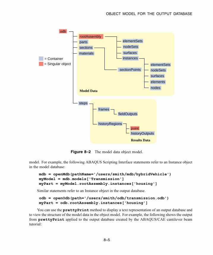
OBJECT MODEL FOR THE OUTPUT DATABASE
steps
frames
historyRegions
fieldOutputs
pointhistoryOutputs
= Container = Singular object
odb
nodeSets
elementSets
surfaces
instances
nodeSets
elementSets
surfaces
elements
nodes
rootAssembly
parts
sections
sectionPoints
Model Data
Results Data
materials
Figure 8–2 The model data object model.
model. For example, the following ABAQUS Scripting Interface statements refer to an Instance object
in the model database:
mdb = openMdb(pathName='/users/smith/mdb/hybridVehicle')myModel = mdb.models['Transmission']myPart = myModel.rootAssembly.instances['housing']
Similar statements refer to an Instance object in the output database.
odb = openOdb(path='/users/smith/odb/transmission.odb')myPart = odb.rootAssembly.instances['housing']
You can use the prettyPrint method to display a text representation of an output database and
to view the structure of the model data in the object model. For example, the following shows the output
from prettyPrint applied to the output database created by the ABAQUS/CAE cantilever beam
tutorial:
8–5
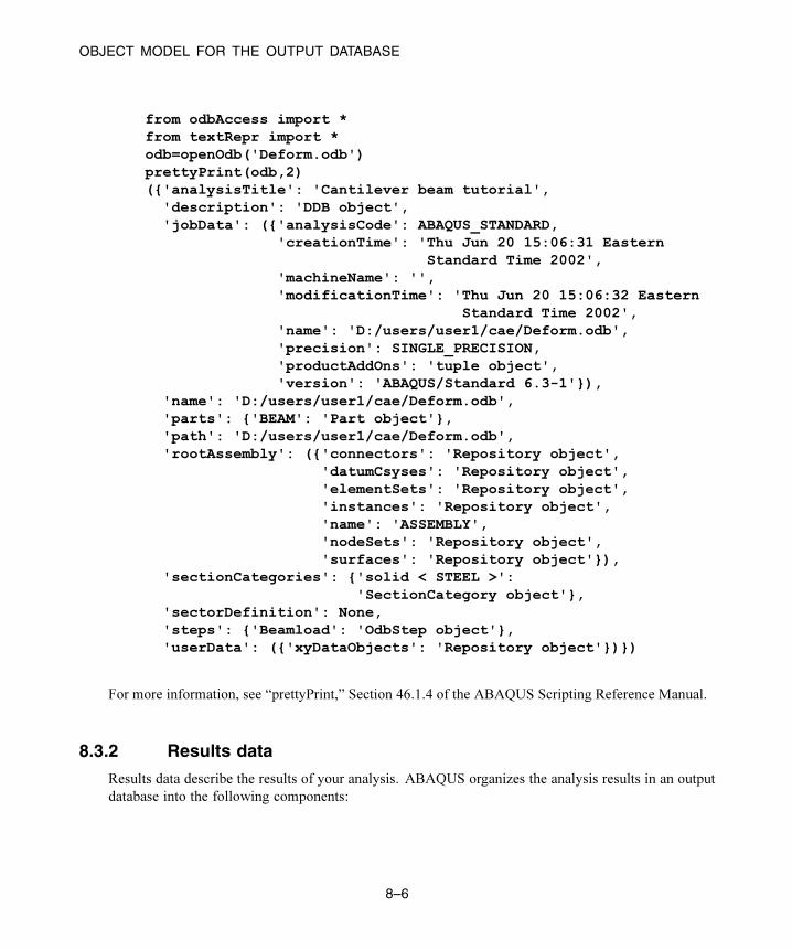
OBJECT MODEL FOR THE OUTPUT DATABASE
from odbAccess import *from textRepr import *odb=openOdb('Deform.odb')prettyPrint(odb,2)({'analysisTitle': 'Cantilever beam tutorial',
'description': 'DDB object','jobData': ({'analysisCode': ABAQUS_STANDARD,
'creationTime': 'Thu Jun 20 15:06:31 EasternStandard Time 2002',
'machineName': '','modificationTime': 'Thu Jun 20 15:06:32 Eastern
Standard Time 2002','name': 'D:/users/user1/cae/Deform.odb','precision': SINGLE_PRECISION,'productAddOns': 'tuple object','version': 'ABAQUS/Standard 6.3-1'}),
'name': 'D:/users/user1/cae/Deform.odb','parts': {'BEAM': 'Part object'},'path': 'D:/users/user1/cae/Deform.odb','rootAssembly': ({'connectors': 'Repository object',
'datumCsyses': 'Repository object','elementSets': 'Repository object','instances': 'Repository object','name': 'ASSEMBLY','nodeSets': 'Repository object','surfaces': 'Repository object'}),
'sectionCategories': {'solid < STEEL >':'SectionCategory object'},
'sectorDefinition': None,'steps': {'Beamload': 'OdbStep object'},'userData': ({'xyDataObjects': 'Repository object'})})
For more information, see “prettyPrint,” Section 46.1.4 of the ABAQUS Scripting Reference Manual.
8.3.2 Results data
Results data describe the results of your analysis. ABAQUS organizes the analysis results in an output
database into the following components:
8–6

OBJECT MODEL FOR THE OUTPUT DATABASE
Steps
An ABAQUS analysis contains a sequence of one or more analysis steps. Each step is associated
with an analysis procedure.
Frames
Each step contains a sequence of frames, where each increment of the analysis that resulted in output
to the output database is called a frame. In a frequency or buckling analysis each eigenmode is stored
as a separate frame. Similarly, in a steady-state harmonic response analysis each frequency is stored
as a separate frame.
Field output
Field output is intended for infrequent requests for a large portion of the model and can be used to
generate contour plots, animations, symbol plots, and displaced shape plots in the Visualization
module of ABAQUS/CAE. You can also use field output to generate an X–Y data plot. Only
complete sets of basic variables (for example, all the stress or strain components) can be requested
as field output. Field output is composed of a “cloud of data values” (e.g., stress tensors at each
integration point for all elements). Each data value has a location, type, and value. You use the
regions defined in the model data, such as an element set, to access subsets of the field output data.
Figure 8–3 shows the field output data object model within an output database.
steps
historyRegions
= Container = Singular object
odbrootAssembly
parts
sections
Model Data
Results Data
frames
fieldValuesfieldOutputs
materials
Figure 8–3 The field output data object model.
History output
History output is output defined for a single point or for values calculated for a portion of the model
as a whole, such as energy. History output is intended for relatively frequent output requests for
small portions of the model and can be displayed in the form of X–Y data plots in the Visualization
8–7

EXECUTING A SCRIPT THAT ACCESSES AN OUTPUT DATABASE
module of ABAQUS/CAE. Individual variables (such as a particular stress component) can be
requested.
Depending on the type of output expected, a HistoryRegion object can be defined for one of
the following:
• a node
• an integration point
• a region
• the whole model
The output from all history requests that relate to a particular point or region is then collected in
one HistoryRegion object. Figure 8–4 shows the history output data object model within an output
database.
steps
frames
= Container = Singular object
odbrootAssembly
parts
data
sections
Model Data
Results Data
historyRegionspoint
historyOutputs
fieldOutputs
materials
Figure 8–4 The history output data.
8.4 Executing a script that accesses an output database
If your script accesses and manipulates data in an output database, you can use either of the following
methods to execute the script:
• Type abaqus python scriptname.py at the system prompt.
• Select File→Run Script from the ABAQUS/CAE main menu bar, and select the file to execute.
8–8

READING FROM AN OUTPUT DATABASE
Your script must contain the following statement:
from odbAccess import *
In addition, if your script refers to any of the Symbolic Constants defined in the ABAQUS Scripting
Interface, your script must contain the following statement:
from abaqusConstants import *
If your script accesses or creates material objects, or if it accesses or creates section or beam profile
objects, it must contain the following statements, respectively:
from odbMaterial import *from odbSection import *
8.5 Reading from an output database
The following sections describe how you use ABAQUS Scripting Interface commands to read data from
an output database. The following topics are covered:
• “The ABAQUS/CAE Visualization module tutorial output database,” Section 8.5.1
• “Making the Odb commands available,” Section 8.5.2
• “Opening an output database,” Section 8.5.3
• “Reading model data,” Section 8.5.4
• “Reading results data,” Section 8.5.5
• “Reading field output data,” Section 8.5.6
• “Using regions to read a subset of field output data,” Section 8.5.7
• “Reading history output data,” Section 8.5.8
• “An example of reading node and element information from an output database,” Section 8.5.9
• “An example of reading field data from an output database,” Section 8.5.10
8.5.1 The ABAQUS/CAE Visualization module tutorial output database
The following sections describe how you can access the data in an output database. Examples
are included that refer to the ABAQUS/CAE Visualization module tutorial output database,
viewer_tutorial.odb. This database is generated by the input file from Case 2 of the example
problem, “Indentation of an elastomeric foam specimen with a hemispherical punch,” Section 1.1.4
of the ABAQUS Example Problems Manual. The problem studies the behavior of a soft elastomeric
foam block indented by a heavy metal punch. The tutorial shows how you can use the Visualization
module to view the data in the output database. The tutorial describes how you can choose the variable
8–9
READING FROM AN OUTPUT DATABASE
to display, how you can step through the steps and frames in the analysis, and how you can create X–Y
data from history output.
You are encouraged to copy the tutorial output database to a local directory and experiment with
the ABAQUS Scripting Interface. The output database and the example scripts from this manual can be
copied to the user’s working directory using the ABAQUS fetch utility:
abaqus fetch job=name
where name.py is the name of the script or name.odb is the name of the output database (see “Execution
procedure for ABAQUS/Fetch,” Section 3.2.12 of the ABAQUS Analysis User’s Manual). For example,
use the following command to retrieve the tutorial output database:
abaqus fetch job=viewer_tutorial
8.5.2 Making the Odb commands available
To make the Odb commands available to your script, you first need to import the odbAccess module
using the following statements:
from odbAccess import *from abaqusConstants import *
To make the material and section Odb commands available to your script, you also need to import the
relevant module using the following statements:
from odbMaterial import *from odbSection import *
8.5.3 Opening an output database
You use the openOdbmethod to open an existing output database. For example, the following statement
opens the output database used by the ABAQUS/CAE Visualization module tutorial:
odb = openOdb(path='viewer_tutorial.odb')
After you open the output database, you can access its contents using the methods and members of the
Odb object returned by the openOdb method. In the above example the Odb object is referred to by
the variable odb. This odb variable is used in this chapter and in Chapter 30, “Odb commands,” of
the ABAQUS Scripting Reference Manual. For a full description of the openOdb command, see “Odb
commands,” Section 30.26 of the ABAQUS Scripting Reference Manual.
8–10
READING FROM AN OUTPUT DATABASE
8.5.4 Reading model data
The following list describes the objects in model data and the commands you use to read model data.
Many of the objects are repositories, and you will find the keys() method useful for determining the
names of the objects in the repository. For more information, see “Using dictionaries,” Section 4.6.2,
and “Repositories,” Section 5.3.3.
The root assembly
An output database contains only one root assembly. You access the root assembly through the
OdbAssembly object.
myAssembly = odb.rootAssembly
Part instances
Part instances are stored in the instances repository under the OdbAssembly object. The
following statements display the repository keys of the part instances in the tutorial output database:
for instanceName in odb.rootAssembly.instances.keys():print instanceName
The output database contains only one part instance, and the resulting output is
PART-1-1
Regions
Regions in the output database are OdbSet objects. Regions refer to the part and assembly sets stored
in the output database. A part set refers to elements or nodes in an individual part and appears in
each instance of the part in the assembly. An assembly set refers to the elements or nodes in part
instances in the assembly. A region can be one of the following:
• A node set
• An element set
• A surface
For example, the following statement displays the node sets in the OdbAssembly object:
print 'Node sets = ',odb.rootAssembly.nodeSets.keys()
The resulting output is
Node sets = ['ALL NODES']
The following statements display the node sets and the element sets in the PART-1-1 part instance:
print 'Node sets = ',odb.rootAssembly.instances['PART-1-1'].nodeSets.keys()
8–11

READING FROM AN OUTPUT DATABASE
print 'Element sets = ',odb.rootAssembly.instances['PART-1-1'].elementSets.keys()
The resulting output is
Node sets = ['ALLN', 'BOT', 'CENTER', 'N1', 'N19', 'N481','N499', 'PUNCH', 'TOP']
Element sets = ['CENT', 'ETOP', 'FOAM', 'PMASS', 'UPPER']
The following statement assigns a variable (topNodeSet) to the ’TOP’ node set in the PART-1-1 part instance:
topNodeSet = odb.rootAssembly.instances['PART-1-1'].nodeSets['TOP']
The type of the object to which topNodeSet refers is OdbSet. After you create a variable that
refers to a region, you can use the variable to refer to a subset of field output data, as described in
“Using regions to read a subset of field output data,” Section 8.5.7.
Materials
Materials are stored in the materials repository under the Odb object.
Access the materials repository using the command:
allMaterials = odb.materialsfor materialName in allMaterials.keys():
print 'Material Name : ',materialName
To print isotropic elastic material properties in a material object:
for material in allMaterials.values():if hasattr(material,'elastic'):
elastic = material.elasticif elastic.type == ISOTROPIC:
print 'isotropic elastic behavior, type = %s' \% elastic.modulititle1 = 'Young modulus Poisson\'s ratio 'title2 = ''if elastic.temperatureDependency == ON:
title2 = 'Temperature 'dep = elastic.dependenciestitle3 = ''for x in range(dep):
title3 += ' field # %d' % xprint '%s %s %s' % (title1,title2,title3)for dataline in elastic.table:
8–12

READING FROM AN OUTPUT DATABASE
print dataline
Some Material definitions have suboptions. For example, to access the smoothing type used
for biaxial test data specified for a hyperelastic material:
if hasattr(material,'hyperelastic'):hyperelastic = material.hyperelastictestData = hyperelastic.testDataif testData == ON:
if hasattr(hyperelastic,'biaxialTestData'):biaxialTestData = hyperelastic.biaxialTestDataprint 'smoothing type : ',biaxialTestData.smoothing
Chapter 25, “Material commands,” of the ABAQUS Scripting Reference Manual describes the
Material object commands in more detail.
Sections
Sections are stored in the sections repository under the Odb object.
The following statements display the repository keys of the sections in an output database:
allSections = odb.sectionsfor sectionName in allSections.keys():
print 'Section Name : ',sectionName
The Section object can be one of the various section types. The type command provides
information on the section type. For example, to determine whether a section is of type
“homogeneous solid section” and to print it’s thickness and associated material name:
for mySection in allSections.values():if type(mySection) == HomogeneousSolidSectionType:
print 'material name = ', mySection.materialprint 'thickness = ', mySection.thickness
Similarily, to access the beam profile repository:
allProfiles = odb.profiles.values()numProfiles = len(allProfiles)print 'Total Number of profiles in the ODB : %d' \
% numProfiles
The Profile object can be one of the various profile types. The type command provides
information on the profile type. For example, to output the radius of all circular profiles in the odb:
for myProfile in allProfiles:if type(myProfile) == CircularProfileType:
print 'profile name = %s, radius = %8.3f' \
8–13

READING FROM AN OUTPUT DATABASE
% (myProfile.name,myProfile.r)
Section assignments
Section assignments are stored in the sectionAssignments repository under the OdbAssembly
object.
All elements in an ABAQUS analysis need to be associated with section and material
properties. Section assignments provide the relationship between elements in a part instance and
their section properties. The section properties include the associated material name. To access the
sectionAssignments repository from the PartInstance object:
instances = odb.rootAssembly.instancesfor instance in instances.values():
assignments = instance.sectionAssignmentsprint 'Instance : ',instance.namefor sa in assignments:
region = sa.regionelements = region.elementsmySection = sa.sectionprint ' Section : ',mySection.nameprint ' Elements associated with this section : 'for e in elements:
print ' label : ',e.label
8.5.5 Reading results data
The following list describes the objects in results data and the commands you use to read results data.
As with model data you will find it useful to use the keys()method to determine the keys of the results
data repositories.
Steps
Steps are stored in the steps repository under the Odb object. The key to the steps repository
is the name of the step. The following statements print out the keys of each step in the repository:
for stepName in odb.steps.keys():print stepName
The resulting output is
Step-1Step-2Step-3
Note: An index of 0 in a sequence refers to the first value in the sequence, and an index of −1 refers
to the last value. You can use the following syntax to refer to an individual item in a repository:
8–14

READING FROM AN OUTPUT DATABASE
step1 = odb.steps.values()[0]print step1.name
The resulting output is
Step-1
Frames
Each step contains a sequence of frames, where each increment of the analysis (or each mode in an
eigenvalue analysis) that resulted in output to the output database is called a frame. The following
statement assigns a variable to the last frame in the first step:
lastFrame = odb.steps['Step-1'].frames[-1]
8.5.6 Reading field output data
Field output data are stored in the fieldOutputs repository under the OdbFrame object. The key to
the repository is the name of the variable. The following statements list all the variables found in the last
frame of the first step (the statements use the variable lastFrame that we defined previously):
for fieldName in lastFrame.fieldOutputs.keys():print fieldName
COPEN TARGET/IMPACTORCPRESS TARGET/IMPACTORCSHEAR1 TARGET/IMPACTORCSLIP1 TARGET/IMPACTORLERFRM3SUUR3
Different variables can be written to the output database at different frequencies. As a result, not all
frames will contain all the field output variables.
You can use the following to view all the available field data in a frame:
# For each field output value in the last frame,# print the name, description, and type members.
for f in lastFrame.fieldOutputs.values():print f.name, ':', f.description
8–15

READING FROM AN OUTPUT DATABASE
print 'Type: ', f.type
# For each location value, print the position.
for loc in f.locations:print 'Position:',loc.position
The resulting print output lists all the field output variables in a particular frame, along with their type
and position.
COPEN TARGET/IMPACTOR : Contact openingType: SCALARPosition: NODAL
CPRESS TARGET/IMPACTOR : Contact pressureType: SCALARPosition: NODAL
CSHEAR1 TARGET/IMPACTOR : Frictional shearType: SCALARPosition: NODAL
CSLIP1 TARGET/IMPACTOR : Relative tangential motion direction 1Type: SCALARPosition: NODAL
LE : Logarithmic strain componentsType: TENSOR_2D_PLANARPosition: INTEGRATION_POINT
RF : Reaction forceType: VECTORPosition: NODAL
RM3 : Reaction momentType: SCALARPosition: NODAL
S : Stress componentsType: TENSOR_2D_PLANARPosition: INTEGRATION_POINT
8–16

READING FROM AN OUTPUT DATABASE
U : Spatial displacementType: VECTORPosition: NODAL
UR3 : Rotational displacementType: SCALARPosition: NODAL
In turn, a FieldOutput object has a member values that is a sequence of FieldValue objects that
contain data. Each data value in the sequence has a particular location in the model. You can query the
FieldValue object to determine the location of a data value; for example,
displacement=lastFrame.fieldOutputs['U']fieldValues=displacement.values
# For each displacement value, print the nodeLabel# and data members.
for v in fieldValues:print 'Node = %d U[x] = %6.4f, U[y] = %6.4f' % (v.nodeLabel,v.data[0], v.data[1])
The resulting output is
Node = 1 U[x] = 0.0000, U[y] = -76.4580Node = 3 U[x] = -0.0000, U[y] = -64.6314Node = 5 U[x] = 0.0000, U[y] = -52.0814Node = 7 U[x] = -0.0000, U[y] = -39.6389Node = 9 U[x] = -0.0000, U[y] = -28.7779Node = 11 U[x] = -0.0000, U[y] = -20.3237...
The data in the FieldValue object depend on the field output variable, which is displacement in the above
example. The following command lists all the members of a particular FieldValue object:
fieldValues[0].__members__
The resulting output is
['instance', 'elementLabel', 'nodeLabel', 'position','face', 'integrationPoint', 'sectionPoint',
'localCoordSystem', 'type', 'data', 'magnitude','mises', 'tresca', 'press', 'inv3', 'maxPrincipal','midPrincipal', 'minPrincipal', 'maxInPlanePrincipal',
8–17
READING FROM AN OUTPUT DATABASE
'minInPlanePrincipal', 'outOfPlanePrincipal']
Where applicable, you can obtain section point information from the FieldValue object.
8.5.7 Using regions to read a subset of field output data
After you have created an OdbSet object using model data, you can use the getSubsetmethod to read
only the data corresponding to that region. Typically, you will be reading data from a region that refers to
a node set or an element set. For example, the following statements create a variable called center that
refers to the node set PUNCH at the center of the hemispherical punch. In a previous section you created
the displacement variable that refers to the displacement of the entire model in the final frame of the
first step. Now you use the getSubset command to get the displacement for only the center region.
center = odb.rootAssembly.instances['PART-1-1'].nodeSets['PUNCH']centerDisplacement = displacement.getSubset(region=center)centerValues = centerDisplacement.valuesfor v in centerValues:
print v.nodeLabel, v.data
The resulting output is
1000 array([0.0000, -76.4555], 'd')
The arguments to getSubset are a region, an element type, a position, or section point data. The
following is a second example that uses an element set to define the region and generates formatted output.
For more information on tuples, the len() function, and the range() function, see “Sequences,”
Section 4.5.4, and “Sequence operations,” Section 4.5.5.
topCenter = \odb.rootAssembly.instances['PART-1-1'].elementSets['CENT']
stressField = odb.steps['Step-2'].frames[3].fieldOutputs['S']
# The following variable represents the stress at# integration points for CAX4 elements from the# element set "CENT."
field = stressField.getSubset(region=topCenter,position=INTEGRATION_POINT, elementType = CAX4)
fieldValues = field.valuesfor v in fieldValues:
print 'Element label = ', v.elementLabels,if v.integrationPoint:
print 'Integration Point = ', v.integrationPointelse:
8–18

READING FROM AN OUTPUT DATABASE
print# For each tensor component.
for component in v.data:
# Print using a format. The comma at the end of the# print statement suppresses the carriage return.
print '%-10.5f' % component,
# After each tuple has printed, print a carriage return.
The resulting output is
Element label = 1 Integration Point = 1S : 0.01230 -0.05658 0.00892 -0.00015Element label = 1 Integration Point = 2S : 0.01313 -0.05659 0.00892 -0.00106Element label = 1 Integration Point = 3S : 0.00619 -0.05642 0.00892 -0.00023Element label = 1 Integration Point = 4S : 0.00697 -0.05642 0.00892 -0.00108Element label = 11 Integration Point = 1S : 0.01281 -0.05660 0.00897 -0.00146Element label = 11 Integration Point = 2S : 0.01183 -0.05651 0.00897 -0.00257Element label = 11 Integration Point = 3 ...
Possible values for the position argument to the getSubset command are:
• INTEGRATION_POINT
• NODAL
• ELEMENT_NODAL
• CENTROID
If the requested field values are not found in the output database at the specified ELEMENT_NODAL or
CENTROID positions, they are extrapolated from the field data at the INTEGRATION_POINT position.
8–19

READING FROM AN OUTPUT DATABASE
8.5.8 Reading history output data
History output is output defined for a single point or for values calculated for a portion of the model as
a whole, such as energy. Depending on the type of output expected, the historyRegions repository
contains data from one of the following:
• a node
• an integration point
• a region
• a material point
Note: History data from an analysis cannot contain multiple points.
The history data object model is shown in Figure 8–5.
steps
frames
= Container = Singular object
odbrootAssembly
parts
data
sections
Model Data
Results Data
historyRegionspoint
historyOutputs
fieldOutputs
materials
Figure 8–5 The history data object model.
In contrast to field output, which is associated with a frame, history output is associated with a step.
History output data are stored in the historyRegions repository under an OdbStep object. ABAQUS
creates keys to the historyRegions repository that describe the region; for example,
• ’Node PART-1-1.1000’
• ’Element PART-1-1.2 Int Point 1’
• ’Assembly rootAssembly’
8–20

READING FROM AN OUTPUT DATABASE
The output from all history requests that relate to a specified point is collected in one HistoryRegion
object. A HistoryRegion object contains multiple HistoryOutput objects. Each HistoryOutput object, in
turn, contains a sequence of (frameValue, value) sequences. In a time domain analysis (domain=TIME)
the sequence is a tuple of (stepTime, value). In a frequency domain analysis (domain=FREQUENCY) the
sequence is a tuple of (frequency, value). In a modal domain analysis (domain=MODAL) the sequence
is a tuple of (mode, value).
In the analysis that generated the ABAQUS/CAE Visualization module tutorial output database, the
user asked for the following history output:
At the rigid body reference point (Node 1000)
• U
• V
• A
At the corner element
• MISES
• LE22
• S22
The history output data can be retrieved from the HistoryRegion objects in the output database. The
tutorial output database contains HistoryRegion objects that relate to the rigid body reference point and
the integration points of the corner element as follows:
• ’Node PART-1-1.1000’
• ’Element PART-1-1.1 Int Point 1’
• ’Element PART-1-1.1 Int Point 2’
• ’Element PART-1-1.1 Int Point 3’
• ’Element PART-1-1.1 Int Point 4’
The following statements read the tutorial output database and write the U2 history data from the second
step to an ASCII file that can be plotted by ABAQUS/CAE:
from odbAccess import *
odb = openOdb(path='viewer_tutorial.odb')step2 = odb.steps['Step-2']region = step2.historyRegions['Node PART-1-1.1000']u2Data = region.historyOutputs['U2'].datadispFile = open('disp.dat','w')for time, u2Disp in u2Data:
dispFile.write('%10.4E %10.4E\n' % (time, u2Disp))dispFile.close()
8–21

READING FROM AN OUTPUT DATABASE
The output in this example is a sequence of tuples containing the frame time and the displacement value.
The example uses nodal history data output. If the analysis requested history output from an element, the
output database would contain one HistoryRegion object and one HistoryPoint object for each integration
point.
8.5.9 An example of reading node and element information from an
output database
The following script illustrates how you can open the output database used by the ABAQUS/CAE
Visualization module tutorial output database and print out some nodal and element information. Use
the following commands to retrieve the example script and the tutorial output database:
abaqus fetch job=odbElementConnectivityabaqus fetch job=viewer_tutorial
# odbElementConnectivity.py# Script to extract node and element information.## Command line argument is the path to the output# database.## For each node of each part instance:# Print the node label and the nodal coordinates.## For each element of each part instance:# Print the element label, the element type, the# number of nodes, and the element connectivity.
from odbAccess import *import sys
# Check that an output database was specified.
if len(sys.argv) != 2:print 'Error: you must supply the name \
of an odb on the command line'sys.exit(1)
# Get the command line argument.
odbPath = sys.argv[1]
8–22

READING FROM AN OUTPUT DATABASE
# Open the output database.
odb = openOdb(path=odbPath)
assembly = odb.rootAssembly
# Model data output
print 'Model data for ODB: ', odbPath
# For each instance in the assembly.
numNodes = numElements = 0
for name, instance in assembly.instances.items():
n = len(instance.nodes)print 'Number of nodes of instance %s: %d' % (name, n)numNodes = numNodes + n
printprint 'NODAL COORDINATES'
# For each node of each part instance# print the node label and the nodal coordinates.# Three-dimensional parts include X-, Y-, and Z-coordinates.# Two-dimensional parts include X- and Y-coordinates.
if instance.embeddedSpace == THREE_D:print ' X Y Z'for node in instance.nodes:
print node.coordinateselse:
print ' X Y'for node in instance.nodes:
print node.coordinates
# For each element of each part instance# print the element label, the element type, the# number of nodes, and the element connectivity.
8–23

READING FROM AN OUTPUT DATABASE
n = len(instance.elements)print 'Number of elements of instance ', name, ': ', nnumElements = numElements + n
print 'ELEMENT CONNECTIVITY'print ' Number Type Connectivity'for element in instance.elements:
print '%5d %8s' % (element.label, element.type),for nodeNum in element.connectivity:
print '%4d' % nodeNum,print
printprint 'Number of instances: ', len(assembly.instances)print 'Total number of elements: ', numElementsprint 'Total number of nodes: ', numNodes
8.5.10 An example of reading field data from an output database
The following script combines many of the commands you have already seen and illustrates how you
read model data and field output data from the output database used by the ABAQUS/CAE Visualization
module tutorial. Use the following commands to retrieve the example script and the tutorial output
database:
abaqus fetch job=odbReadabaqus fetch job=viewer_tutorial
# odbRead.py# A script to read the ABAQUS/CAE Visualization module tutorial# output database and read displacement data from the node at# the center of the hemispherical punch.
from odbAccess import *
odb = openOdb(path='viewer_tutorial.odb')
# Create a variable that refers to the# last frame of the first step.
8–24

READING FROM AN OUTPUT DATABASE
lastFrame = odb.steps['Step-1'].frames[-1]
# Create a variable that refers to the displacement 'U'# in the last frame of the first step.
displacement = lastFrame.fieldOutputs['U']
# Create a variable that refers to the node set 'PUNCH'# located at the center of the hemispherical punch.# The set is associated with the part instance 'PART-1-1'.
center = odb.rootAssembly.instances['PART-1-1'].\nodeSets['PUNCH']
# Create a variable that refers to the displacement of the node# set in the last frame of the first step.
centerDisplacement = displacement.getSubset(region=center)
# Finally, print some field output data from each node# in the node set (a single node in this example).
for v in centerDisplacement.values:print 'Position = ', v.position,'Type = ',v.typeprint 'Node label = ', v.nodeLabelprint 'X displacement = ', v.data[0]print 'Y displacement = ', v.data[1]print 'Displacement magnitude =', v.magnitude
odb.close()
The resulting output is
Position = NODAL Type = VECTORNode label = 1000X displacement = -8.29017850095e-34Y displacement = -76.4554519653Displacement magnitude = 76.4554519653
8–25
WRITING TO AN OUTPUT DATABASE
8.6 Writing to an output database
You can write your own data to an output database, and you can use ABAQUS/CAE to view the data.
Writing to an output database is very similar to reading from an output database. When you open an
existing database, the Odb object contains all the objects found in the output database, such as instances,
steps, and field output data. In contrast, when you are writing to a new output database, these objects do
not exist. As a result you must use a constructor to create the objects. For example, you use the Partconstructor to create a Part object, the Instance constructor to create an OdbInstance object, and the
Step constructor to create an OdbStep object.
After you create an object, you use methods of the objects to enter or modify the data associated
with the object. For example, if you are creating an output database, you first create an Odb object.
You then use the Part constructor to create a part. After creating the part, you use the addNodes and
addElements methods of the Part object to add nodes and elements, respectively. Similarly, you use
the addData method of the FieldOutput object to add field output data to the output database. After
creating an output database, you should use the save method on the Odb object to save the output
database.
The example script in “Creating an output database,” Section 8.10.2, also illustrates how you can
write to an output database.
The following topics are covered:
• “Creating a new output database,” Section 8.6.1
• “Writing model data,” Section 8.6.2
• “Writing results data,” Section 8.6.3
• “Writing field output data,” Section 8.6.4
• “Default display properties,” Section 8.6.5
• “Writing history output data,” Section 8.6.6
8.6.1 Creating a new output database
You use the Odb constructor to create a new, empty Odb object.
odb = Odb(name='myData',analysisTitle='derived data',description='test problem',path='testWrite.odb')
For a full description of the Odb command, see “Odb,” Section 30.1.1 of the ABAQUS Scripting
Reference Manual. ABAQUS creates the RootAssembly object when you create or open an output
database.
8–26
WRITING TO AN OUTPUT DATABASE
You use the save method to save the output database.
odb.save()
For a full description of the save command, see “save,” Section 30.1.4 of the ABAQUS Scripting
Reference Manual.
8.6.2 Writing model data
To define the geometry of your model, you first create the parts that are used by the model and then you
add nodes and elements to the parts. You then define the assembly by creating instances of the parts. If
the output database already contains results data, you should not change the geometry of the model. This
is to ensure that the results remain synchronized with the model.
Part
If the part was created by ABAQUS/CAE, the description of the native ABAQUS/CAE geometry
is stored in the model database, but it is not stored in the output database. A part is stored in
an output database as a collection of nodes, elements, surfaces, and sets. You use the Partconstructor to add a part to the Odb object. You can specify the type of the part; however, only
DEFORMABLE_BODY is currently supported. For example,
part1 = odb.Part(name='part-1',embeddedSpace=THREE_D, type=DEFORMABLE_BODY)
For a full description of the Part constructor, see “OdbPart object,” Section 30.18 of the ABAQUS
Scripting Reference Manual. The new Part object is empty and does not contain geometry. After
you create the Part object, you add nodes and elements.
You use the addNodes method to add nodes by defining node labels and coordinates. You
can also define an optional node set. For example,
nodeData = ( (1, 1,0,0), (2, 2,0,0),(3, 2,1,0.1), (4, 1,1,0.1),(5, 2,-1,-0.1), (6, 1,-1,-0.1), )
part1.addNodes(nodeData=nodeData, nodeSetName='nset-1')
For a full description of the addNodes command, see “addNodes,” Section 30.18.4 of the
ABAQUS Scripting Reference Manual.
After you have created nodes, you can use the NodeSetFromNodeLabels constructor to
create a node set from the node labels. For more information, see “NodeSetFromNodeLabels,”
Section 30.19.2 of the ABAQUS Scripting Reference Manual.
Similarly, you use the addElements method to add elements to the part using a sequence
of element labels, element connectivity, and element type. You can also define an optional element
set and an optional section category. For example,
# Set up the section categories
8–27

WRITING TO AN OUTPUT DATABASE
sCat = odb.SectionCategory(name='S5',description='Five-Layered Shell')
spBot = sCat.SectionPoint(number=1,description='Bottom')
spMid = sCat.SectionPoint(number=3,description='Middle')
spTop = sCat.SectionPoint(number=5,description='Top')
elementData = ((1, 1,2,3,4),(2, 6,5,2,1),)
part1.addElements(elementData=elementData, type='S4',elementSetName='eset-1', sectionCategory=sCat)
For a full description of the addElements command, see “addElements,” Section 30.18.2 of the
ABAQUS Scripting Reference Manual.
The RootAssembly object
The root assembly is created when you create the output database. You access the RootAssembly
object using the same syntax as that used for reading from an output database.
odb.rootAssembly
You can create both instances and regions on the RootAssembly object.
Part instances
You use the Instance constructor to create part instances of the parts you have already defined
using the Part constructor. For example,
a = odb.rootAssemblyinstance1 = a.Instance(name='part-1-1', object=part1)
You can also supply an optional local coordinate system that specifies the rotation and translation
of the part instance. You can add nodes and elements only to a part; you cannot add elements
and nodes to a part instance. As a result, you should create the nodes and elements that define the
geometry of a part before you instance the part. For a full description of the Instance command,
see “OdbInstance object,” Section 30.14 of the ABAQUS Scripting Reference Manual.
Regions
Region commands are used to create sets from element labels, node labels, and element faces. You
can create a set on a part, part instance, or the root assembly. Node and element labels are unique
8–28

WRITING TO AN OUTPUT DATABASE
within an instance but not within the assembly. As a result, a set on the root assembly requires
the names of the part instances associated with the nodes and elements. You can also use region
commands to create surfaces. For example,
# An element set on an instanceeLabels = [9,99]elementSet = instance1.ElementSetFromElementLabels(
name='elsetA',elementLabels=eLabels)# A node set on the rootAssemblynodeLabels = (5,11)instanceName = 'part-1-1'nodeSet = assembly.NodeSetFromNodeLabels(
name='nodesetRA',((instanceName,nodeLabels),))
The region commands are described in Chapter 39, “Region commands,” of the ABAQUS
Scripting Reference Manual.
Materials
You use the Material object to list material properties.
Materials are stored in the materials repository under the Odb object.
To create an isotropic elastic material, with a Young’s modulus of 12000.0 and an effective
Poisson’s ratio of 0.3 in the output database:
materialName = "Elastic Material"material_1 = odb.Material(name=materialName)material_1.Elastic(type=ISOTROPIC,table=((12000,0.3),))
For more information, see Chapter 25, “Material commands,” of the ABAQUS Scripting
Reference Manual.
Sections
You use the Section object to create sections and profiles.
Sections are stored in the sections repository under the Odb object.
The following code creates a homogeneous solid section object. A Material object must be
present before creating a Section object. An exception is thrown if the material does not exist.
sectionName = 'Homogeneous Solid Section'mySection = odb.HomogeneousSolidSection( name = sectionName,
material = materialName,thickness = 2.0)
To create a circular beam profile object in the output database:
profileName = "Circular Profile"radius = 10.00
8–29

WRITING TO AN OUTPUT DATABASE
odb.CircularProfile(name = profileName, r = radius)
Section assignments
You use the SectionAssignment object to assign sections and their associated material properties
to regions of the model. SectionAssignment objects are members of the Odb object. For a full
description of the assignSection method, see “assignSection,” Section 30.14.7 of the ABAQUS
Scripting Reference Manual.
All Elements in an ABAQUS analysis need to be associated with section and material
properties. Section assignments provide the relationship between elements in an Instance object
and their section properties. The section properties include the associated material name. To create
an element set and assign a section:
elLabels = (1,2)elset = instance.ElementSetFromElementLabels(
name=materialName, elementLabels=elLabels)instance.assignSection(region=elset,section=section)
8.6.3 Writing results data
To write results data to the output database, you first create the Step objects that correspond to each step
of the analysis. If you are writing field output data, you also create the Frame objects that will contain
the field data. History output data are associated with Step objects.
Steps
You use the Step constructor to create a results step for time, frequency, or modal domain results.
For example,
step1 = odb.Step(name='step-1',description='', domain=TIME, timePeriod=1.0)
The Step constructor has an optional previousStepName argument that specifies the step after
which this step must be inserted in the steps repository. For a full description of the Stepcommand, see “Step,” Section 30.20.1 of the ABAQUS Scripting Reference Manual.
Frames
You use the Frame constructor to create a frame for field output. For example,
frame1 = step1.Frame(frameId=1,frameValue=0.1, description='')
For a full description of the Frame command, see “Frame,” Section 30.13.3 of the ABAQUS
Scripting Reference Manual.
8–30

WRITING TO AN OUTPUT DATABASE
8.6.4 Writing field output data
A FieldOutput object contains a “cloud of data values” (e.g., stress tensors at each integration point for
all elements). Each data value has a location, type, and value. You add field output data to a Frame object
by first creating a FieldOutput object using the FieldOutput constructor and then adding data to the
FieldOutput object using the addData method. For example,
# Create the part and the instance.
part1 = odb.Part(name='part-1',embeddedSpace=THREE_D, type=DEFORMABLE_BODY)
a = odb.rootAssemblyinstance1 = a.Instance(name='part-1-1', object=part1)
# Write nodal displacements
uField = frame1.FieldOutput(name='U',description='Displacements', type=VECTOR)
# Create the node labels.
nodeLabelData = (1, 2, 3, 4, 5, 6)
# Each set of data corresponds to a node label.
dispData = ((1,2,3),(4,5,6),(7,8,9),(10,11,12),(13, 14, 15),(16,17,18))
# Add nodal data to the FieldOutput object using the# node labels and the nodal data for this part instance.
uField.addData(position=NODAL, instance=instance1,labels=nodeLabelData, data=dispData)
# Make this the default deformed field for this step.
8–31

WRITING TO AN OUTPUT DATABASE
step1.setDefaultDeformedField(uField)
For a full description of the FieldOutput constructor, see “FieldOutput,” Section 30.3.1 of the
ABAQUS Scripting Reference Manual.
The type argument to the FieldOutput constructor describes the type of the data—tensor, vector,
or scalar. The properties of the different tensor types are:
Full tensor
A tensor that has six components and three principal values. Full three-dimensional rotation of the
tensor is possible.
Three-dimensional surface tensor
A tensor that has only three in-plane components and two principal values. Full three-dimensional
rotation of the tensor components is possible.
Three-dimensional planar tensor
A tensor that has three in-plane components, one out-of-plane component, and three principal
values. Full three-dimensional rotation of the tensor components is possible.
Two-dimensional surface tensor
A tensor that has only three in-plane components and two principal values. Only in-plane rotation
of the tensor components is possible.
Two-dimensional planar tensor
A tensor that has three in-plane components, one out-of-plane component, and three principal
values. Only in-plane rotation of the tensor components is possible.
The valid components and invariants for the different data types are given in Table 8–1.
Table 8–1 Valid components and invariants for ABAQUS data types.
Data type Components Invariants
SCALAR
VECTOR 1, 2, 3 MAGNITUDE
TENSOR_3D_FULL 11, 22, 33, 12, 13, 23 MISES, TRESCA, PRESS, INV3,
MAX_PRINCIPAL, MID_PRINCIPAL,
MIN_PRINCIPAL
TENSOR_3D_SURFACE 11, 22, 12 MAX_PRINCIPAL, MIN_PRINCIPAL,
MAX_INPLANE_PRINCIPAL,
MIN_INPLANE_PRINCIPAL
8–32

WRITING TO AN OUTPUT DATABASE
Data type Components Invariants
TENSOR_3D_PLANAR 11, 22, 33, 12 MISES, TRESCA, PRESS,
INV3, MAX_PRINCIPAL,
MID_PRINCIPAL, MIN_PRINCIPAL,
MAX_INPLANE_PRINCIPAL,
MIN_INPLANE_PRINCIPAL,
OUTOFPLANE_PRINCIPAL
TENSOR_2D_SURFACE 11, 22, 12 MAX_PRINCIPAL, MIN_PRINCIPAL,
MAX_INPLANE_PRINCIPAL,
MIN_INPLANE_PRINCIPAL
TENSOR_2D_PLANAR 11, 22, 33, 12 MISES, TRESCA, PRESS,
INV3, MAX_PRINCIPAL,
MID_PRINCIPAL, MIN_PRINCIPAL,
MAX_INPLANE_PRINCIPAL,
MIN_INPLANE_PRINCIPAL,
OUTOFPLANE_PRINCIPAL
For example, the following statements add element data to the FieldOutput object:
# Write stress tensors (output only available at# top/bottom section points)# The element defined above (S4) has 4 integration# points. Hence, there are 4 stress tensors per element.# ABAQUS creates one layer of section points each# time the script calls the addData method.
elementLabelData = (1, 2)
topData = ((1.,2.,3.,4.), (1.,2.,3.,4.),(1.,2.,3.,4.), (1.,2.,3.,4.),(1.,2.,3.,4.), (1.,2.,3.,4.),(1.,2.,3.,4.), (1.,2.,3.,4.),
)bottomData = ((1.,2.,3.,4.), (1.,2.,3.,4.),
(1.,2.,3.,4.), (1.,2.,3.,4.),(1.,2.,3.,4.), (1.,2.,3.,4.),(1.,2.,3.,4.), (1.,2.,3.,4.),
)
transform = ((1.,0.,0.), (0.,1.,0.), (0.,0.,1.))
8–33

WRITING TO AN OUTPUT DATABASE
sField = frame1.FieldOutput(name='S',description='Stress', type=TENSOR_3D_PLANAR,componentLabels=('S11', 'S22', 'S33','S12'), validInvariants=(MISES,))
sField.addData(position=INTEGRATION_POINT,sectionPoint=spTop, instance=instance1,labels=elementLabelData, data=topData,localCoordSystem=transform)
sField.addData(position=INTEGRATION_POINT,sectionPoint=spBot, instance=instance1,labels=elementLabelData, data=bottomData,localCoordSystem=transform)
# For this step, make this the default field for# visualization.
step1.setDefaultField(sField)
For a full description of the addData command, see “addData,” Section 30.3.3 of the ABAQUS
Scripting Reference Manual.
As a convenience, localCoordSystem can be a single transform or a list of transforms. If
localCoordSystem is a single transform, it applies to all values. If localCoordSystem is a list of
transforms, the number of items in the list must match the number of data values.
8.6.5 Default display properties
The previous examples show how you can use commands to set the default field variable and deformed
field variable. ABAQUS/CAE uses the default field variable setting to determine the variable to display in
a contour plot; for example, stress. Similarly, the default deformed field variable determines the variable
that distinguishes a deformed plot from an undeformed plot. Typically, you will use displacement for the
default deformed field variable; you cannot specify an invariant or a component. The default variable
settings apply for each frame in the step. For example, the following statements use the deformation ’U’as the default setting for both field variable and deformed field variable settings during a particular step:
field=odb.steps['impact'].frames[1].fieldOutputs['U']odb.steps['impact'].setDefaultField(field)odb.steps['impact'].setDefaultDeformedField(field)
You can set a different default field variable and deformed field variable for different steps. You
will need to use a loop to set the defaults for each step. For example,
for step in odb.steps.values():
8–34
WRITING TO AN OUTPUT DATABASE
step.setDefaultField(field)
8.6.6 Writing history output data
History output is output defined for a single point or for values calculated for a portion of the model as
a whole, such as energy. Depending on the type of output expected, the historyRegions repository
contains data from one of the following:
• a node
• an element, or a location in an element
• a region
Note: History data from an analysis cannot contain multiple points.
The output from all history requests that relate to a specified point is collected in one HistoryRegion
object. You use the HistoryPoint constructor to create the point. For example,
point1 = HistoryPoint(element=instance1.elements[0])
For a full description of the HistoryPoint command, see “HistoryPoint,” Section 30.6.1 of the
ABAQUS Scripting Reference Manual.
You then use the HistoryRegion constructor to create a HistoryRegion object:
step1 = odb.Step(name='step-1',description='', domain=TIME, timePeriod=1.0)
h1 = step1.HistoryRegion(name='my history',description='my stuff',point=point1)
For a full description of the HistoryRegion command, see “HistoryRegion,” Section 30.7.1 of the
ABAQUS Scripting Reference Manual.
You use the HistoryOutput constructor to add variables to the HistoryRegion object.
h1_u1 = h1.HistoryOutput(name='U1',description='Displacement', type=SCALAR)
h1_rf1 = h1.HistoryOutput(name='RF1',description='Reaction Force', type=SCALAR)
# Similarly for Step 2
step2 = odb.Step(name='step-2',description='', domain=TIME, timePeriod=1.0)
h2 = step2.HistoryRegion(name='my history',description='my stuff', point=point1)
h2_u1 = h2.HistoryOutput(name='U1',description='Displacement', type=SCALAR)
8–35

EXCEPTION HANDLING IN AN OUTPUT DATABASE
h2_rf1 = h2.HistoryOutput(name='RF1',description='Reaction Force', type=SCALAR)
Each HistoryOutput object contains a sequence of (frameValue, value) sequences. The
HistoryOutput object has a method (addData) for adding data. Each data item is a sequence of
(frameValue, value). In a time domain analysis (domain=TIME) the sequence is (stepTime, value). In
a frequency domain analysis (domain=FREQUENCY) the sequence is (frequency, value). In a modal
domain analysis (domain=MODAL) the sequence is (mode, value).
You add the data values as time and data tuples. The number of data items must correspond to the
number of time items. For example,
timeData = (0.0, 0.1, 0.3, 1.0)u1Data = (0.0, 0.0004, 0.0067, 0.0514)rf1Data = (27.456, 32.555, 8.967, 41.222)
h1_u1.addData(frameValue=timeData, value=u1Data)h1_rf1.addData(frameValue=timeData, value=rf1Data)
# similar for step2
timeData = (1.2, 1.9, 3.0, 4.0)u1Data = (0.8, 0.9, 1.3, 1.5)rf1Data = (0.9, 1.1, 1.3, 1.5)
h2_u1.addData(frameValue=timeData, value=u1Data)h2_rf1.addData(frameValue=timeData, value=rf1Data)
8.7 Exception handling in an output database
Python exception handling is described in “Exception handling,” Section 5.5.4. Python exception
handling in the output database is identical to that in the model database. The exceptions thrown are of
type OdbError; for example, the following script catches exceptions thrown when the python interface
in not successful in opening an output database:
invalidOdbName = "invalid.odb"try:
myOdb = openOdb(invalidOdbName)except OdbError,e:print 'Abaqus error message: %s' % str(e)print 'customized error message here'
except:
8–36

COMPUTATIONS WITH ABAQUS RESULTS
print 'Unknown Exception. '
8.8 Computations with ABAQUS results
The following topics are covered:
• “Rules for the mathematical operations,” Section 8.8.1
• “Valid mathematical operations,” Section 8.8.2
• “Envelope calculations,” Section 8.8.3
8.8.1 Rules for the mathematical operations
Mathematical operations are supported for FieldOutput, FieldValue, and HistoryOutput objects. These
operators allow you to perform linear superposition of ABAQUS results or to create more complex
derived results from ABAQUS results.
The following rules apply:
• The operations are performed on the components of a tensor or vector.
• The invariants are computed from the component values. For example, taking the absolute value
of a tensor can result in negative values of the pressure invariant.
• Operations between FieldOutput, FieldValue, and HistoryOutput objects are not supported.
• Multiplication and division are not supported between two vector objects nor between two tensor
objects.
• The types in an expression must be compatible. For example,
– A vector cannot be added to a tensor.
– A three-dimensional surface tensor cannot be added to a three-dimensional planar tensor.
– INTEGRATION_POINT data cannot be added to ELEMENT_NODAL data.
• If the fields in the expression were obtained using the getSubsetmethod, the same getSubsetoperations must have been applied in the same order to obtain each field.
• Arguments to the trigonometric functions must be in radians.
• Operations on tensors are performed in the local coordinate system, if it is available. Otherwise
the global system is used. ABAQUS assumes that the local coordinate systems are consistent for
operations involving more than one tensor.
• Operations between FieldValue objects associated with different locations in the model are allowed
only if the data types are the same. If the locations in the model differ, the FieldValue computed
will not be associated with a location. If the local coordinate systems of the FieldValue objects are
8–37

COMPUTATIONS WITH ABAQUS RESULTS
not the same, the local coordinate systems of both fieldValues will be disregarded and the fieldValue
computed will have no local coordinate system.
• The operations will not be performed on the conjugate data (the imaginary portion of a complex
result).
The FieldOutput operations are significantly more efficient than the FieldValue operators. You can
save the computed FieldOutput objects with the following procedure (see the example, “Computations
with FieldOutput objects,” Section 8.10.4):
• Create a new FieldOutput object in the output database.
• Use the addData method to add the new computed field objects to the new FieldOutput object.
8.8.2 Valid mathematical operations
Table 8–2 describes the abbreviations that are used in mathematical operations.
Table 8–2 Abbreviations.
Abbreviation Allowable values
all FieldOutput objects, FieldValue objects, HistoryVariable
objects, or floating point numbers
float floating point numbers
FO FieldOutput objects
FV FieldValue objects
HO HistoryOutput objects
Table 8–3 shows the valid operations on FieldOutput objects.
Table 8–3 Valid operations.
Symbol Operation Return
value
all + float addition all
FO + FO FO
FV + FV FV
HO + HO HO
-all unary negation all
8–38

COMPUTATIONS WITH ABAQUS RESULTS
Symbol Operation Return
value
all - float subtraction all
FO - FO FO
FV - FV FV
HO + HO HO
all * float multiplication all
all / float division all
abs(all) absolute value all
acos(all) arccosine all
asin(all) arcsine all
atan(all) arctangent all
cos(all) cosine all
degreeToRadian
(all)
convert degrees to
radians
all
exp(all) natural exponent all
exp10(all) base 10 exponent all
log(all) natural logarithm all
log10(all) base 10 logarithm all
float ** float raise to a power all
power(FO, float) FO
power(FV, float) FV
power(HO, float) HO
radianToDegree
(all)
convert radian to
degree
all
sin(all) sine all
sqrt(all) square root all
tan(all) tangent all
8–39
COMPUTATIONS WITH ABAQUS RESULTS
8.8.3 Envelope calculations
You use envelope calculations to retrieve the extreme value for an output variable over a number of
fields. Envelope calculations are especially useful for retrieving the extreme values over a number of
load cases.
The following operators consider a list of fields and perform the envelope calculation:
(env, lcIndex) = maxEnvelope([field1, field2, ...])(env, lcIndex) = minEnvelope([field1, field2, ...])
(env, lcIndex) = maxEnvelope([field1, field2, ...],invariant)
(env, lcIndex) = minEnvelope([field1, field2, ...],invariant)
(env, lcIndex) = maxEnvelope([field1, field2, ...],componentLabel)
(env, lcIndex) = minEnvelope([field1, field2, ...],componentLabel)
The envelope commands return two FieldOutput objects.
• The first object contains the requested extreme values.
• The second object contains the indices of the fields for which the extreme values were found. The
indices derive from the order in which you supplied the fields to the command.
The optional invariant argument is a Symbolic Constant specifying the invariant to be used when
comparing vectors or tensors. The optional componentLabel argument is a String specifying the
component of the vector or tensor to be used for selecting the extreme value.
The following rules apply to envelope calculations:
• ABAQUS compares the values using scalar data. If you are looking for the extreme value of a vector
or a tensor, you must supply an invariant or a component label for the selection of the extreme value.
For example, for vectors you can supply the MAGNITUDE invariant and for tensors you can supply
the MISES invariant.
• The fields being compared must be similar. For example,
– VECTOR and TENSOR_3D_FULL fields cannot appear in the same list.
– The output region of all the fields must be the same. All the fields must apply to the whole
model, or all the fields must apply to the same set.
8–40

COMPUTATIONS WITH ABAQUS RESULTS
8.8.4 Transformation of results
Transformations of vector and tensor fields are supported for rectangular, cylindrical, and spherical
coordinate systems. The coordinate systems can be fixed or model based. Model-based coordinate
systems refer to nodes for position and orientation. ABAQUS uses the coordinates of the deformed state
to determine a systems origin and orientation for model-based coordinate systems. Transformations
that use a model-based coordinate system can account for large displacements of both the coordinate
system and the structure.
The steps required to transform results are (see also the example “Transformation of field results,”
Section 8.10.10):
• Create the coordinate system.
• Retrieve the field from the database.
• Use the fieldOutput.getTransformedFieldmethod to obtain a new field with the results
in the specified coordinate system.
• For large displacement of the structure and coordinate system, you must also retrieve the
displacement field at the frame. You must compute this displacement field for the whole model to
ensure that the required displacement information is available.
The following rules apply to the transformation of results:
• Beams, truss, and axisymmetric shell element results will not be transformed.
• The component directions 1, 2, and 3 of the transformed results will correspond to the system
directions X, Y, and Z for rectangular coordinate systems; R, , and Z for cylindrical coordinate
systems; and R, , and for spherical coordinate systems.
Note: Stress results for three-dimensional continuum elements transformed into a cylindrical
system would have the hoop stress in S22, which is consistent with the coordinate system axis
but inconsistent with the stress state for a three-dimensional axisymmetric elements having hoop
stress in S33.
• When you are transforming a tensor, the location or integration point always takes into account the
deformation. The location of the coordinate system depends on the model, as follows:
– If the system is fixed, the coordinate system is fixed.
– If the system is model based, you must supply a displacement field that determines the
instantaneous location and orientation of the coordinate system.
• ABAQUSwill perform transformations of tensor results for shells, membranes, and planar elements
as rotations of results about the element normal at the element result location. The element normal is
the normal computed for the frame associated with the field by ABAQUS, and you cannot redefine
the normal. ABAQUS defines the location of the results location from the nodal locations. You
specify optional arguments if you want to use the deformed nodal locations to transform results.
8–41

IMPROVING THE EFFICIENCY OF YOUR SCRIPTS
For rectangular, cylindrical, and spherical coordinate systems the second component direction for
the transformed results will be determined by one of the following:
– The Y-axis in a rectangular coordinate system.
– The -axis in a cylindrical coordinate system.
– The -axis in a spherical coordinate system.
– A user-specified datum axis projected onto the element plane.
If the coordinate system used for projection and the element normal have an angle less than the
specified tolerance (the default is 30°), ABAQUS will use the next axis and generate a warning.
8.9 Improving the efficiency of your scripts
If you are accessing large amounts of data from an output database, you should be aware of potential
inefficiencies in your script and techniques that will help to speed up your scripts.
• “Creating objects to hold temporary variables,” Section 8.9.1
8.9.1 Creating objects to hold temporary variables
To improve the efficiency of scripts that access an output database, you should create objects that will
be used to hold temporary variables that are accessed multiple times while the script is executing. For
example, if the script accesses the temporary variable while inside a loop that is executed many times,
creating an object to hold the variable will speed up your script significantly.
The following example examines the von Mises stress in each element during a particular frame of
field output. If the stress is greater than a certain maximum value, the script prints the strain components
for the element.
stressField = frame.fieldOutputs['MISES']strainField = frame.fieldOutputs['LE']count = 0for v in stressField.values():
if v.mises > stressCap:if v.integrationPoint:
print 'Element label = ', v.elementLabel, \'Integration Point = ', v.integrationPoint
else:print 'Element label = ', v.elementLabel
for component in strainField.values[count].data:print '%-10.5f' % component,
8–42

IMPROVING THE EFFICIENCY OF YOUR SCRIPTS
printcount = count + 1
In this example every time the script accesses a strain component from strainField.value, ABAQUS
must reconstruct the sequence of FieldValue objects. This reconstruction could result in a significant
performance degradation, particularly for a large model.
A slight change in the script greatly improves its performance, as shown in the following example:
stressField = frame.fieldOutputs['MISES']strainFieldValues = frame.fieldOutputs['LE'].valuescount = 0for v in stressField.values():
if v.mises > stressCap:if v.integrationPoint:
print 'Element label = ', v.elementLabel, \'Integration Point = ', v.integrationPoint
else:print 'Element label = ', v.elementLabel
for component in strainFieldValues[count].data:print '%-10.5f' % component,
printcount = count + 1
The second script replaces the statement strainField = frame.fieldOutputs[’LE’]with the statement strainFieldValues = frame.fieldOutputs[’LE’].values. As a
result, ABAQUS does not need to reconstruct the sequence of FieldValue objects each time the script
accesses a strain component.
Similarly, if you expect to retrieve more than one frame from an output database, you should create
a temporary variable that holds the entire frame repository. You can then provide the logic to retrieve the
desired frames from the repository and avoid recreating the repository each time. For example, executing
the following statements could be very slow:
for i in range(len(odb.steps[name].frames)-1):frame[i] = odb.steps[name].frames[i]
Creating a temporary variable to hold the frame repository provides the same functionality and speeds
up the process:
frameRepository = odb.steps[name].framesfor i in range(len(frameRepository)-1):
frame[i] = frameRepository[i]
Such a potential loss of performance will not be a problem when accessing a load case frame. Accessing
a load case frame does not result in the creation of a frame repository and, thus, does not suffer from a
corresponding loss of performance.
8–43

EXAMPLE SCRIPTS THAT ACCESS DATA FROM AN OUTPUT DATABASE
8.10 Example scripts that access data from an output database
The following examples illustrate how you use the output database commands to access data from an
output database:
• “Finding the maximum value of von Mises stress,” Section 8.10.1
• “Creating an output database,” Section 8.10.2
• “An ABAQUS Scripting Interface version of FPERT,” Section 8.10.3
• “Computations with FieldOutput objects,” Section 8.10.4
• “Computations with FieldValue objects,” Section 8.10.5
• “Computations with HistoryOutput objects,” Section 8.10.6
• “Adding results from one output database into another output database,” Section 8.10.7
• “Creating a new load combination from different load cases,” Section 8.10.8
• “Stress range for multiple load cases,” Section 8.10.9
• “Transformation of field results,” Section 8.10.10
• “Viewing the analysis of a meshed beam cross-section,” Section 8.10.11
• “Using infinite elements to compute and view the results of an acoustic far-field analysis,”
Section 8.10.12
• “An ABAQUS Scripting Interface version of FELBOW,” Section 8.10.13
In addition, the ABAQUS Scripting Interface examples, “Reading from an output database,” Section 3.2,
and “Investigating the skew sensitivity of shell elements,” Section 7.3, illustrate how to read data from
an output database.
8.10.1 Finding the maximum value of von Mises stress
This example illustrates how you can iterate through an output database and search for the maximum
value of von Mises stress. The script opens the output database specified by the first argument on the
command line and iterates through the following:
• Each step.
• Each frame in each step.
• Each value of von Mises stress in each frame.
In addition, you can supply an optional assembly element set argument from the command line, in which
case the script searches only the element set for the maximum value of von Mises stress.
The following illustrates how you can run the example script from the system prompt. The script
will search the element set ALL ELEMENTS in the viewer tutorial output database for the maximum
value of von Mises stress:
8–44

EXAMPLE SCRIPTS THAT ACCESS DATA FROM AN OUTPUT DATABASE
abaqus python odbMaxMises.py -odb viewer_tutorial.odb-elset “ ALL ELEMENTS”
Note: If a command line argument is a String that contains spaces, some systems will interpret the String
correctly only if it is enclosed in double quotation marks. For example, “ ALL ELEMENTS”.
You can also run the example with only the -help parameter for a summary of the usage.
Use the following commands to retrieve the example script and the viewer tutorial output database:
abaqus fetch job=odbMaxMises.pyabaqus fetch job=viewer_tutorial
"""odbMaxMises.pyCode to determine the location and value of the maximumvon-mises stress in an output database.Usage: abaqus python odbMaxMises.py -odb odbName
-elset(optional) elsetNameRequirements:1. -odb : Name of the output database.2. -elset : Name of the assembly level element set.
Search will be done only for element belongingto this set. If this parameter is not provided,search will be performed over the entire model.
3. -help : Print usage"""
#~~~~~~~~~~~~~~~~~~~~~~~~~~~~~~~~~~~~~~~~~~~~~~~~~~~~~~~~~~~~~from odbAccess import *from sys import argv,exit#~~~~~~~~~~~~~~~~~~~~~~~~~~~~~~~~~~~~~~~~~~~~~~~~~~~~~~~~~~~~~
def rightTrim(input,suffix):if (input.find(suffix) == -1):
input = input + suffixreturn input
#~~~~~~~~~~~~~~~~~~~~~~~~~~~~~~~~~~~~~~~~~~~~~~~~~~~~~~~~~~~~~
def getMaxMises(odbName,elsetName):""" Print max mises location and value given odbName
and elset(optional)"""elset = elemset = None
8–45

EXAMPLE SCRIPTS THAT ACCESS DATA FROM AN OUTPUT DATABASE
region = "over the entire model"""" Open the output database """odb = openOdb(odbName)assembly = odb.rootAssembly
""" Check to see if the element set existsin the assembly
"""if elsetName:
try:elemset = assembly.elementSets[elsetName]region = " in the element set : " + elsetName;
except KeyError:print 'An assembly level elset named %s does' \
'not exist in the output database %s' \% (elsetName, odbName)
odb.close()exit(0)
""" Initialize maximum values """maxMises = -0.1maxElem = 0maxStep = "_None_"maxFrame = -1Stress = 'S'isStressPresent = 0for step in odb.steps.values():
print 'Processing Step:', step.namefor frame in step.frames:
allFields = frame.fieldOutputsif (allFields.has_key(Stress)):
isStressPresent = 1stressSet = allFields[Stress]if elemset:
stressSet = stressSet.getSubset(region=elemset)
for stressValue in stressSet.values:if (stressValue.mises > maxMises):
maxMises = stressValue.misesmaxElem = stressValue.elementLabelmaxStep = step.name
8–46

EXAMPLE SCRIPTS THAT ACCESS DATA FROM AN OUTPUT DATABASE
maxFrame = frame.frameIdif(isStressPresent):
print 'Maximum von Mises stress %s is %f in element %d'%(region, maxMises, maxElem)
print 'Location: frame # %d step: %s '%(maxFrame,maxStep)else:
print 'Stress output is not available in' \'the output database : %s\n' %(odb.name)
""" Close the output database before exiting the program """odb.close()
#==================================================================# S T A R T#if __name__ == '__main__':
odbName = NoneelsetName = NoneargList = argvargc = len(argList)i=0while (i < argc):
if (argList[i][:2] == "-o"):i += 1name = argList[i]odbName = rightTrim(name,".odb")
elif (argList[i][:2] == "-e"):i += 1elsetName = argList[i]
elif (argList[i][:2] == "-h"):print __doc__exit(0)
i += 1if not (odbName):
print ' **ERROR** output database name is not provided'print __doc__exit(1)
getMaxMises(odbName,elsetName)
8–47
EXAMPLE SCRIPTS THAT ACCESS DATA FROM AN OUTPUT DATABASE
8.10.2 Creating an output database
The following example illustrates how you can use the ABAQUS Scripting Interface commands to do
the following:
1. Create a new output database.
2. Add model data.
3. Add field data.
4. Add history data.
5. Read history data.
6. Save the output database.
Use the following command to retrieve the example script:
abaqus fetch job=odbWrite
"""odbWrite.pyScript to create an output database and add model,field, and history data. The script also readshistory data, performs an operation on the data, and writesthe result back to the output database.usage: abaqus python odbWrite.py
"""from odbAccess import *from odbMaterial import *from odbSection import *from abaqusConstants import *
def createODB():
# Create an ODB (which also creates the rootAssembly)odb = Odb(name='simpleModel',
analysisTitle='ODB created with Python ODB API',description='example illustrating Python ODB API ',path='odbWritePython.odb')
# create few materialsmaterialName = "Elastic Material"material_1 = odb.Material(name=materialName)
8–48

EXAMPLE SCRIPTS THAT ACCESS DATA FROM AN OUTPUT DATABASE
material_1.Elastic(type=ISOTROPIC,temperatureDependency=OFF, dependencies=0,noCompression=OFF, noTension=OFF,moduli=LONG_TERM, table=((12000,0.3),))
# create few sectionssectionName = 'Homogeneous Solid Section'section_1 = odb.HomogeneousSolidSection(name=sectionName,
material=materialName, thickness=2.0)# Model data:
# Set up the section categories.sCat = odb.SectionCategory(name='S5',
description='Five-Layered Shell')spBot = sCat.SectionPoint(number=1,
description='Bottom')spMid = sCat.SectionPoint(number=3,
description='Middle')spTop = sCat.SectionPoint(number=5,
description='Top')
# Create a 2-element shell model,# 4 integration points, 5 section points.
part1 = odb.Part(name='part-1', embeddedSpace=THREE_D,type=DEFORMABLE_BODY)
nodeData = ((1, 1,0,0),(2, 2,0,0),(3, 2,1,0.1),(4, 1,1,0.1),(5, 2,-1,-0.1),(6, 1,-1,-0.1),)
part1.addNodes(nodeData=nodeData,nodeSetName='nset-1')
elementData = ((1, 1,2,3,4),(2, 6,5,2,1),)
8–49

EXAMPLE SCRIPTS THAT ACCESS DATA FROM AN OUTPUT DATABASE
part1.addElements(elementData=elementData, type='S4',elementSetName='eset-1', sectionCategory=sCat)
# Instance the part.instance1 = odb.rootAssembly.Instance(name='part-1-1',
object=part1)# create instance level sets for section assignmentelLabels = (1,2)elset_1 = odb.rootAssembly.instances['part-1-1'].\
ElementSetFromElementLabels(name=materialName,elementLabels=elLabels)
instance1.assignSection(region=elset_1,section=section_1)
# Field data:
# Create a step and a frame.
step1 = odb.Step(name='step-1',description='first analysis step',domain=TIME, timePeriod=1.0)
analysisTime=0.1frame1 = step1.Frame(frameId=1,
frameValue=analysisTime,description=\
'results frame for time '+str(analysisTime))
# Write nodal displacements.
uField = frame1.FieldOutput(name='U',description='Displacements', type=VECTOR)
nodeLabelData = (1, 2, 3, 4, 5, 6)dispData = (
(1,2,3),(4,5,6),(7,8,9),(10,11,12),(13, 14, 15),(16,17,18)
8–50

EXAMPLE SCRIPTS THAT ACCESS DATA FROM AN OUTPUT DATABASE
)
uField.addData(position=NODAL, instance=instance1,labels=nodeLabelData,data=dispData)
# Make this the default deformed field for visualization.
step1.setDefaultDeformedField(uField)
""" Write stress tensors(output only available at top/bottom section points)The element defined above (S4) has 4 integration points.Hence, there are 4 stress tensors per element.Each Field constructor refers to only one layer of sectionpoints."""
elementLabelData = (1, 2)topData = (
(1.,2.,3.,4.),(1.,2.,3.,4.),(1.,2.,3.,4.),(1.,2.,3.,4.),(1.,2.,3.,4.),(1.,2.,3.,4.),(1.,2.,3.,4.),(1.,2.,3.,4.),)
bottomData = ((1.,2.,3.,4.),(1.,2.,3.,4.),(1.,2.,3.,4.),(1.,2.,3.,4.),(1.,2.,3.,4.),(1.,2.,3.,4.),(1.,2.,3.,4.),(1.,2.,3.,4.),)
transform = (
8–51

EXAMPLE SCRIPTS THAT ACCESS DATA FROM AN OUTPUT DATABASE
(1.,0.,0.),(0.,1.,0.),(0.,0.,1.))
sField = frame1.FieldOutput(name='S',description='Stress', type=TENSOR_3D_PLANAR,componentLabels=('S11', 'S22', 'S33','S12'),validInvariants=(MISES,))
sField.addData(position=INTEGRATION_POINT,sectionPoint=spTop, instance=instance1,labels=elementLabelData, data=topData,localCoordSystem=transform)
sField.addData(position=INTEGRATION_POINT,sectionPoint=spBot, instance=instance1,labels=elementLabelData, data=bottomData,localCoordSystem=transform)
# For this step, make this the default field# for visualization.
step1.setDefaultField(sField)
# History data:
# Create a HistoryRegion for a specific point.
hRegionStep1 = step1.HistoryRegion(name='historyNode0',description='Displacement and reaction force',point=instance1.nodes[0])
# Create variables for this history output in step1.
hOutputStep1U1 = hRegionStep1.HistoryOutput(name='U1',description='Displacement', type=SCALAR)
hOutputStep1Rf1 = hRegionStep1.HistoryOutput(name='RF1',description='Reaction Force', type=SCALAR)
# Add history data for step1.
timeData1 = (0.0, 0.1, 0.3, 1.0)
8–52

EXAMPLE SCRIPTS THAT ACCESS DATA FROM AN OUTPUT DATABASE
u1Data = (0.0, 0.1, 0.3, 0.5)rf1Data = (0.0, 0.1, 0.3, 0.5)
hOutputStep1U1.addData(frameValue=timeData1,value=u1Data)
hOutputStep1Rf1.addData(frameValue=timeData1,value=rf1Data)
# Create another step for history data.step2 = odb.Step(name='step-2', description='',
domain=TIME, timePeriod=1.0)hRegionStep2 = step2.HistoryRegion(
name='historyNode0',description='Displacement and reaction force',point=instance1.nodes[0])
hOutputStep2U1 = hRegionStep2.HistoryOutput(name='U1',description='Displacement',type=SCALAR)
hOutputStep2Rf1 = hRegionStep2.HistoryOutput(name='RF1',description='Reaction Force',type=SCALAR)
# Add history data for the second step.timeData2 = (1.2, 1.9, 3.0, 4.0)u1Data = (0.8, 0.9, 1.3, 1.5)rf1Data = (0.9, 1.1, 1.3, 1.5)
hOutputStep2U1.addData(frameValue=timeData2,value=u1Data)
hOutputStep2Rf1.addData(frameValue=timeData2,value=rf1Data)
# Get XY Data from the two steps.u1FromStep1 = hRegionStep1.getSubset(variableName='U1')u1FromStep2 = hRegionStep2.getSubset(variableName='U1')
# Square the history data.u1SquaredFromStep1 = \
power(u1FromStep1.historyOutputs['U1'], 2.0)
8–53
EXAMPLE SCRIPTS THAT ACCESS DATA FROM AN OUTPUT DATABASE
u1SquaredFromStep2 = \power(u1FromStep2.historyOutputs['U1'], 2.0)
# Add the squared displacement to the two steps.hOutputStep1sumU1 = hRegionStep1.HistoryOutput(
name='squareU1',description='Square of displacements',type=SCALAR)
hOutputStep1sumU1.addData(data=u1SquaredFromStep1.data)
hOutputStep2sumU1 = hRegionStep2.HistoryOutput(name='squareU1',description='Square of displacements',type=SCALAR)
hOutputStep2sumU1.addData(data=u1SquaredFromStep2.data)
# Save the results in the output database.# Use the Visualization module of ABAQUS/CAE to# view the contents of the output database.
odb.save()
if __name__ == "__main__":createODB()
8.10.3 An ABAQUS Scripting Interface version of FPERT
A FORTRAN program that reads the ABAQUS results file and creates a deformedmesh from the original
coordinate data and eigenvectors is described in “Creation of a perturbed mesh from original coordinate
data and eigenvectors: FPERT,” Section 12.1.4 of the ABAQUS Example Problems Manual. This
example illustrates an ABAQUS Scripting Interface script that reads an output database and performs
similar calculations.
The command line arguments provide the following:
• odbName: The output database file name.
• modeList: A list of eigenmodes to use in the perturbation.
• weightList: The perturbation weighting factors.
8–54

EXAMPLE SCRIPTS THAT ACCESS DATA FROM AN OUTPUT DATABASE
• outNameUser: The output file name (optional).
Use the following command to retrieve the example script:
abaqus fetch job=odbPert
# ABAQUS Scripting Interface version of FPERT, a FORTRAN# program to create a perturbed mesh from original coordinate# data and eigenvectors. FPERT is described in the ABAQUS Example# Problems Manual.
import sysfrom odbAccess import *from types import IntType
# Get input from the user
odbName = raw_input('Enter odb name (w/o .odb): ')modes = eval(raw_input('Enter mode shape(s): '))if type(modes) is IntType:
modes = (modes,)
odb = openOdb(odbName + '.odb')
# Get the undeformed coordinates from the first# step and frame
step = odb.steps.values()[0]
try:coords = step.frames[0].fieldOutputs['COORD']
except:err = "The analysis must include a field output request \
for variable COORD."print errsys.exit(1)
# Perturb the nodal coordinates
factors = []for mode in modes:
8–55

EXAMPLE SCRIPTS THAT ACCESS DATA FROM AN OUTPUT DATABASE
try:frame = step.frames[mode]
except IndexError:print 'Input error: mode %s does not exist' % modesys.exit(1)
factors.append(float(raw_input('Enter imperfection factor for mode %s: '% mode)))
coords = coords + factors[-1] * frame.fieldOutputs['U']
# Write new nodal coordinates to a file
outFile = open(odbName + '_perturbed.inp', 'w')header = \"""********************************************************* Node data for perturbed mesh.** Input mesh from: %s** Mode shapes used: %s** Imperfection factors used: %s*******************************************************"""outFile.write(header % (odbName, modes, factors))format = '%6i, %14.7e, %14.7e, %14.7e\n'for value in coords.values:
outFile.write(format % ((value.nodeLabel,) + tuple(value.data)))
outFile.write('** End of perturbed mesh node input file.')outFile.close()
8.10.4 Computations with FieldOutput objects
This example illustrates how you can operate on FieldOutput objects and save the computed field to the
output database. The example script does the following:
• Retrieves two specified fields from the output database.
• Computes a new field by subtracting the fields that were retrieved.
• Creates a new Step object in the output database.
• Creates a new Frame object in the new step.
• Creates a new FieldOutput object in the new frame.
8–56

EXAMPLE SCRIPTS THAT ACCESS DATA FROM AN OUTPUT DATABASE
• Uses the addData method to add the computed field to the new FieldOutput object.
Use the following command to retrieve the example script:
abaqus fetch job=fieldOperation
The fetch command also retrieves an input file that you can use to generate the output database that is
read by the example script.
# FieldOutput operators example problem## Script that does computations with fields and# saves the results computed to the output database#
from odbAccess import *odb = openOdb(path='fieldOperation.odb')
# Get fields from output database.
field1 = odb.steps['LC1'].frames[1].fieldOutputs['U']field2 = odb.steps['LC2'].frames[1].fieldOutputs['U']
# Compute difference between fields.
deltaDisp = field2 - field1
# Save new field.
newStep = odb.Step(name='user',description='user defined results', domain= TIME, timePeriod=0)
newFrame = newStep.Frame(frameId=0, frameValue=0.0)newField = newFrame.FieldOutput(name='U',
description='delta displacements', type=VECTOR)newField.addData(field=deltaDisp)
odb.save()
8–57

EXAMPLE SCRIPTS THAT ACCESS DATA FROM AN OUTPUT DATABASE
8.10.5 Computations with FieldValue objects
This example illustrates how you can use the fieldValue operators to sum and average fieldValues in a
region. The example script does the following:
• Retrieves the stress field for a specified region during the last step and frame of the output database.
• Sums all the stress fieldValues and computes the average value.
• For each component of stress, print the sum and the average stress.
Use the following command to retrieve the example script:
abaqus fetch job=sumRegionFieldValue
The fetch command also retrieves an input file that you can use to generate the output database that is
read by the example script.
## fieldValue operators example problem:## sum and average stress field values in a region#
from odbAccess import *
## get field#
odb = openOdb(path='sumRegionFieldValue.odb')endSet = odb.rootAssembly.elementSets['END1']field = odb.steps.values()[-1].frames[-1].fieldOutputs['S']subField = field.getSubset(region=endSet)
## sum values#
sum = 0for val in subField.values:
sum = sum + valave = sum / len(subField.values)
8–58

EXAMPLE SCRIPTS THAT ACCESS DATA FROM AN OUTPUT DATABASE
## print results#
print 'Component Sum Average'labels = field.componentLabelsfor i in range( len(labels) ):
print '%s %5.3e %5.3e'% \(labels[i], sum.data[i], ave.data[i])
8.10.6 Computations with HistoryOutput objects
This example illustrates how you can use the historyOutput operators to compute the displacement
magnitude from the components. The example script does the following:
• Retrieves the node of interest using a nodeSet.
• Uses the node of interest to construct a HistoryPoint object.
• Uses the HistoryPoint to retrieve the historyRegion.
• Computes the displacement magnitude history from the displacement component HistoryOutput
objects in the historyRegion.
• Scales the displacement magnitude history using a predefined value.
• Prints the displacement magnitude history.
Use the following command to retrieve the example script:
abaqus fetch job=compDispMagHist
The fetch command also retrieves an input file that you can use to generate the output database that is
read by the example script.
# HistoryOutput operators example problem.## Compute magnitude of node displacement history from# displacement components and scale relative to given# allowable displacement.#
from odbAccess import *
#
8–59

EXAMPLE SCRIPTS THAT ACCESS DATA FROM AN OUTPUT DATABASE
# get historyRegion for the node in nodeSet TIP#
odb = openOdb(path='compDispMagHist.odb')endSet = odb.rootAssembly.instances['BEAM-1-1'].nodeSets['TIP']histPoint = HistoryPoint(node=endSet.nodes[0])tipHistories = odb.steps['Step-2'].getHistoryRegion(
point=histPoint)
## Compute and scale magnitude.#
maxAllowableDisp = 5.0sum = 0componentLabels = ('U1', 'U2', 'U3')for name in componentLabels:
sum = sum + power(tipHistories.historyOutputs[name], 2.0)sum = sqrt(sum) / maxAllowableDisp
## Print magnitude.#
print 'History:', sum.nameprint 'Time Magnitude'for dataPair in sum.data:
print "%5.4f %5.2f"%(dataPair[0], dataPair[1])
8.10.7 Adding results from one output database into another output
database
This example illustrates how you can use the ABAQUS Scripting Interface to extract data from one or
more output databases and write the data sequentially to an existing output database. The following
parameters are required:
8–60

EXAMPLE SCRIPTS THAT ACCESS DATA FROM AN OUTPUT DATABASE
-writeOdb odbName
The name of the output database created by the first analysis. The script creates a copy of this output
database with the name Restart_odbName. All the data read from the other output databases will
be copied into this output database.
-readOdbs odbName
The names of the output databases created by subsequent restart analyses.
The following parameters are optional:
-mergeSteps
You can use this option to merge data when the first step of the restart analysis is a continuation of
a previous analysis step. When you use this option, the script appends all the frames from the first
step in the restart analysis to the corresponding step in Restart_odbName.If you do not specify -mergeSteps, the data from the first step of the restart analysis will be
copied to a new step name stepName-Restart-N, where N is the position of the specified output
database in the list of names of output databases from which data will be copied.
-history
Copy all history output from all available steps. By default, history output is not copied.
WARNING: Copying large amounts of history data can result in the script creating a very large
output database.
-debug
Print a detailed report of all the operations performed during the merging of the output databases.
By default, no debug information is generated.
WARNING: If you are extracting data from a large output database, the -debug parameter can
generate large amounts of information.
You can also run the example with only the -help parameter for a summary of the usage.
The script has the following limitations:
• The script uses the addData method to copy fields from one output database into another; for
more information, see “addData,” Section 30.3.3 of the ABAQUS Scripting Reference Manual.
The addData method requires the model data in the two output databases to be identical. As a
result, the script cannot be used to combine any two output databases. You can use the script with
output databases generated with restart analyses; for more information, see “Restarting an analysis,”
Section 7.1 of the ABAQUS Analysis User’s Manual.
• You can run a restart analysis with additional element and node sets, as described in “Restarting an
analysis,” Section 7.1.1 of the ABAQUS Analysis User’s Manual. However, the odbJoin script
will not copy data from these new sets.
8–61

EXAMPLE SCRIPTS THAT ACCESS DATA FROM AN OUTPUT DATABASE
The following is an example of how you can use this script in conjunction with the output databases
generated by the problem described in “Snap-through buckling analysis of circular arches,” Section 1.2.1
of the ABAQUS Example Problems Manual. Use the following commands to retrieve the script and the
example input files:
abaqus fetch job=odbJoin.pyabaqus fetch job=snapbuckling_shallow_step1.inpabaqus fetch job=snapbuckling_shallow_unload.inp
Run the analysis for the first step and for the subsequent restart analysis. The script will combine the
results across the two resulting output databases:
abaqus job=snapbuckling_shallow_step1.inpabaqus job=snapbuckling_shallow_unload.inp
-oldjob snapbuckling_shallow_step1
Run the script to combine the output databases using the default parameters:
abaqus python odbJoin.py-writeOdb snapbuckling_shallow_step1.odb-readOdbs snapbuckling_shallow_unload.odb
The following is displayed in the message area:
Creating copy of original odb snapbuckling_shallow_step1.odbAll output from restart ODB's will be appended toRestart_snapbuckling_shallow_step1.odbProcessing ODB file snapbuckling_shallow_unload.odbProcessing step Step-2Restart odb files successfully joined intoRestart_snapbuckling_shallow_step1.odb
8.10.8 Creating a new load combination from different load cases
This example illustrates how you can use the frame operators to create a new load combination from
existing load cases. The example script does the following:
• Retrieves the information describing the new load combination from the command line.
• Retrieves the frames for each load case.
• Computes the new stresses and displacements.
• Saves data computed to the output database as a new load combination.
The command line arguments provide the following:
• odbName: The output database file name.
8–62

EXAMPLE SCRIPTS THAT ACCESS DATA FROM AN OUTPUT DATABASE
• stepName: The name of the step containing the load cases.
• loadCaseNames: The load case names.
• scaling: The scale factors to apply to each load case.
Use the following command to retrieve the example script:
abaqus fetch job=createLoadComb
The fetch command also retrieves an input file that you can use to generate an output database that can
be read by the example script.
import typesfrom odbAccess import *
# retrieve request from userodbName = raw_input('Enter odb name')stepName = raw_input('Enter step name')
loadCaseNames = eval(raw_input( \'Enter new load case as: \[\'loadCase1Name\', ..., \'loadCaseNName\']'))
if type(loadCaseNames) == types.TupleType:loadCaseNames = list(loadCaseNames)
lcName = raw_input('Enter new load case name')scaling = eval(raw_input( \
'Enter new load case as:(scaleFactor1, .., scaleFactorN)'))
odb = openOdb(odbName)step = odb.steps[stepName]
# compute new load casenewStress = 0newDisp = 0
for loadCaseName in loadCaseNames:frame = step.getFrame(loadCase=step.loadCases[loadCaseName])scaleFac = scaling[loadCaseNames.index(frame.loadCase.name)]newStress = newStress + scaleFac*frame.fieldOutputs['S']newDisp = newDisp + scaleFac*frame.fieldOutputs['U']
# save new load case to odblcNew = step.LoadCase(name=lcName)
8–63
EXAMPLE SCRIPTS THAT ACCESS DATA FROM AN OUTPUT DATABASE
newFrame = step.Frame(loadCase=lcNew)newFrame.FieldOutput(field=newStress, name='S')newFrame.FieldOutput(name='U', field=newDisp)
odb.save()odb.close()
8.10.9 Stress range for multiple load cases
This example illustrates how you can use the envelope operations to compute the stress range over a
number of load cases. The example script does the following:
• For each load case during a specified step, the script collects the S11 components of the stress tensor
fields into a list of scalar fields.
• Computes the maximum andminimum of the S11 stress component using the envelope calculations.
• Computes the stress range using the maximum and minimum values of the stress component.
• Creates a new frame in the step.
• Writes the computed stress range into a new FieldOutput object in the new frame.
Use the following command to retrieve the example script:
abaqus fetch job=stressRange
The fetch command also retrieves an input file that you can use to generate an output database that can
be read by the example script.
from odbAccess import *
# retrieve request from userodbName = raw_input('Enter odb name')stepName = raw_input('Enter step name')
# retrieve steps from the odbodb=openOdb(odbName)step = odb.steps[stepName]sFields = []
for loadCase in step.loadCases.values():stressField = step.getFrame(loadCase=loadCase).\
fieldOutputs['S']
8–64

EXAMPLE SCRIPTS THAT ACCESS DATA FROM AN OUTPUT DATABASE
sFields.append(stressField.getScalarField(componentLabel='S11'))
# compute stress rangemaxStress, maxLoc = maxEnvelope(sFields)minStress, minLoc = minEnvelope(sFields)
stressRange = maxStress - minStress
# save to same stepnewFrame = step.Frame(frameId=0, frameValue=0.0,
description='Stress Range')newFrame.FieldOutput(field=stressRange, name='S11 Range')
odb.save()odb.close()
8.10.10 Transformation of field results
This example illustrates how field results can be transformed to a different coordinate system. The
example computes deviation of the nodal displacements with respect to a perfectly cylindrical
displacement (cylinder bore distortion). The example does the following:
• Creates a cylindrical coordinate system.
• Transforms the results to the new coordinate system.
• Computes the average radial displacement.
• Computes the distortion as the difference between radial displacement and the average radial
displacement.
• Saves the distortion field to the output database for viewing.
Use the following commands to retrieve the example script and an input file to create a sample
output database:
abaqus fetch job=transformExaabaqus fetch job=esf4sxdg
from odbAccess import *
# Retrieve request from user.
8–65

EXAMPLE SCRIPTS THAT ACCESS DATA FROM AN OUTPUT DATABASE
odbName = raw_input('Enter odb name')stepName = raw_input('Enter step name')frameNo = int( raw_input('Enter frame number') )
odb = openOdb(odbName)
# Retrieve the displacements from last frame of the last step.
step = odb.steps[stepName]frame = step.frames[frameNo]displacement = frame.fieldOutputs['U']
# Create cylindrical coordinate system and compute# associated results
coordSys = odb.rootAssembly.DatumCsysByThreePoints(name='cylC',coordSysType=CYLINDRICAL, origin=(0,0,0),point1=(1.0, 0.0, 0), point2=(0.0, 0.0, 1.0) )
cylindricalDisp = displacement.getTransformedField(datumCsys=coordSys)
radialDisp = cylindricalDisp.getScalarField(componentLabel='U1')
# Compute average radius.
sum = 0.0for val in radialDisp.values:
sum = sum + val.dataaveDisp = sum / len(radialDisp.values)
# Compute distortion.
distortion = radialDisp - aveDisp
# Save computed results to the database.
frame.FieldOutput(field=radialDisp)fieldDescription = 'Distortion ( \
average radial displacement = ' + str(aveDisp) + ')'
8–66

EXAMPLE SCRIPTS THAT ACCESS DATA FROM AN OUTPUT DATABASE
frame.FieldOutput(name='Distortion',description=fieldDescription, field=distortion)
odb.save()odb.close()
8.10.11 Viewing the analysis of a meshed beam cross-section
This example illustrates how you can view the results of a meshed beam cross-section analysis that was
generated using Timoshenko beams, as described in “Meshed beam cross-sections,” Section 7.14 of the
ABAQUS Analysis User’s Manual. Before you execute the example script, you must run two analyses
that create the following output database files:
• An output database generated by the two-dimensional cross-section analysis. The script reads cross-
section data, including the out-of-plane warping function, from this output database.
• An output database generated by the beam analysis. The script reads generalized section strains
(SE) from this output database.
Use the following command to retrieve the example script:
abaqus fetch job=compositeBeam
You must run the script from ABAQUS/CAE by selecting File→Run Script from the main menu bar.
The script usesgetInputs to display a dialog box that prompts you for the name of the output databases
generated by the two-dimensional cross-section analysis and by the beam analysis. The names are
case-insensitive, and you can omit the .odb file suffix. The files must be in the local directory. The
dialog box also prompts you for the following:
• The name of the step
• The increment or mode number (for a frequency analysis)
• The name of the load case (if any)
• The name of the part instance
• The element number
• The integration point number
If you do not enter a value in a field, the script looks in the beam analysis output database for possible
values. The script then enters a default value in the dialog box and displays information about the range
of possible values in the ABAQUS/CAE message area. You can leave the load case field blank if the
analysis did not include load cases. The script does not continue until all the values in the dialog box are
acceptable. The same values are written to a file called compositeBeam_values.dat in the local
directory, and these values appear as defaults in the dialog box the next time you run the example script.
8–67
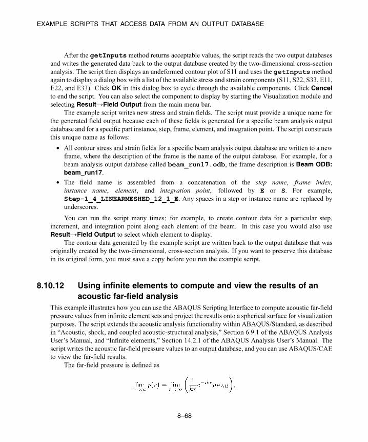
EXAMPLE SCRIPTS THAT ACCESS DATA FROM AN OUTPUT DATABASE
After the getInputs method returns acceptable values, the script reads the two output databases
and writes the generated data back to the output database created by the two-dimensional cross-section
analysis. The script then displays an undeformed contour plot of S11 and uses the getInputs method
again to display a dialog box with a list of the available stress and strain components (S11, S22, S33, E11,
E22, and E33). Click OK in this dialog box to cycle through the available components. Click Cancel
to end the script. You can also select the component to display by starting the Visualization module and
selecting Result→Field Output from the main menu bar.
The example script writes new stress and strain fields. The script must provide a unique name for
the generated field output because each of these fields is generated for a specific beam analysis output
database and for a specific part instance, step, frame, element, and integration point. The script constructs
this unique name as follows:
• All contour stress and strain fields for a specific beam analysis output database are written to a new
frame, where the description of the frame is the name of the output database. For example, for a
beam analysis output database called beam_run17.odb, the frame description is Beam ODB:
beam_run17.
• The field name is assembled from a concatenation of the step name, frame index,
instance name, element, and integration point, followed by E or S. For example,
Step-1_4_LINEARMESHED_12_1_E. Any spaces in a step or instance name are replaced by
underscores.
You can run the script many times; for example, to create contour data for a particular step,
increment, and integration point along each element of the beam. In this case you would also use
Result→Field Output to select which element to display.
The contour data generated by the example script are written back to the output database that was
originally created by the two-dimensional, cross-section analysis. If you want to preserve this database
in its original form, you must save a copy before you run the example script.
8.10.12 Using infinite elements to compute and view the results of an
acoustic far-field analysis
This example illustrates how you can use the ABAQUS Scripting Interface to compute acoustic far-field
pressure values from infinite element sets and project the results onto a spherical surface for visualization
purposes. The script extends the acoustic analysis functionality within ABAQUS/Standard, as described
in “Acoustic, shock, and coupled acoustic-structural analysis,” Section 6.9.1 of the ABAQUS Analysis
User’s Manual, and “Infinite elements,” Section 14.2.1 of the ABAQUS Analysis User’s Manual. The
script writes the acoustic far-field pressure values to an output database, and you can use ABAQUS/CAE
to view the far-field results.
The far-field pressure is defined as
8–68
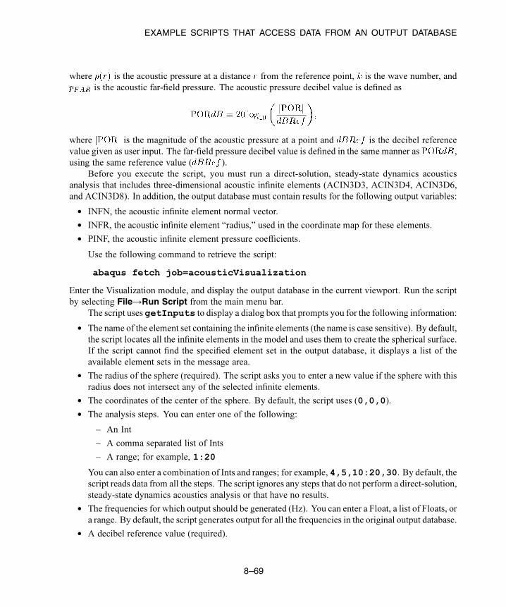
EXAMPLE SCRIPTS THAT ACCESS DATA FROM AN OUTPUT DATABASE
where is the acoustic pressure at a distance from the reference point, is the wave number, and
is the acoustic far-field pressure. The acoustic pressure decibel value is defined as
where is the magnitude of the acoustic pressure at a point and is the decibel reference
value given as user input. The far-field pressure decibel value is defined in the same manner as ,
using the same reference value ( ).
Before you execute the script, you must run a direct-solution, steady-state dynamics acoustics
analysis that includes three-dimensional acoustic infinite elements (ACIN3D3, ACIN3D4, ACIN3D6,
and ACIN3D8). In addition, the output database must contain results for the following output variables:
• INFN, the acoustic infinite element normal vector.
• INFR, the acoustic infinite element “radius,” used in the coordinate map for these elements.
• PINF, the acoustic infinite element pressure coefficients.
Use the following command to retrieve the script:
abaqus fetch job=acousticVisualization
Enter the Visualization module, and display the output database in the current viewport. Run the script
by selecting File→Run Script from the main menu bar.
The script uses getInputs to display a dialog box that prompts you for the following information:
• The name of the element set containing the infinite elements (the name is case sensitive). By default,
the script locates all the infinite elements in the model and uses them to create the spherical surface.
If the script cannot find the specified element set in the output database, it displays a list of the
available element sets in the message area.
• The radius of the sphere (required). The script asks you to enter a new value if the sphere with this
radius does not intersect any of the selected infinite elements.
• The coordinates of the center of the sphere. By default, the script uses (0,0,0).
• The analysis steps. You can enter one of the following:
– An Int
– A comma separated list of Ints
– A range; for example, 1:20
You can also enter a combination of Ints and ranges; for example, 4,5,10:20,30. By default, thescript reads data from all the steps. The script ignores any steps that do not perform a direct-solution,
steady-state dynamics acoustics analysis or that have no results.
• The frequencies for which output should be generated (Hz). You can enter a Float, a list of Floats, or
a range. By default, the script generates output for all the frequencies in the original output database.
• A decibel reference value (required).
8–69
EXAMPLE SCRIPTS THAT ACCESS DATA FROM AN OUTPUT DATABASE
• The name of the part instance to create (required). The script appends this name to the name of the
instance containing the infinite elements being used.
• The speed of sound (required).
• Whether to write data to the original output database. By default, the script writes to an output
database called current-odb-name_acvis.odb.
After the getInputs method returns acceptable values, the script processes the elements in the
specified element sets. The visualization sphere is then determined using the specified radius and center.
For each element in the infinite element sets, the script creates a corresponding membrane element such
that the new element is a projection of the old element onto the surface of the sphere. The projection
uses the infinite element reference point and the internally calculated infinite direction normal (INFN) at
each node of the element.
Once the new display elements have been created, the script writes results at the nodes in the set.
The following output results are written back to the output database:
• POR, the acoustic pressure.
• PORdB, the acoustic pressure decibel value.
• PFAR, the acoustic far-field pressure.
• PFARdB, the far-field pressure decibel value.
To create the output at each node, the script first determines the point at which the node ray intersects
the sphere. Using the distance from the reference point to the intersection point and the element shape
functions, the required output variables are calculated at the intersection point.
After the script has finished writing data, it opens the output database containing the new data. For
comparison, the original instance is displayed along with the new instance, but results are available only
for the new instance. However, if you chose to write the results back to the original output database, the
original instance and the new instance along with the original results and the new results can be displayed
side-by-side. The script displays any error, warning, or information messages in the message area.
You can run the script more than once and continue writing data to the same output database. For
example, you can run the script several times to look at the far-field pressures at various points in space,
and results on several spheres will be written to the output database.
To see how the script operates on a single triangular-element model, use the following command to
retrieve the input file:
abaqus fetch job=singleTriangularElementModel
Use the following command to create the corresponding output database:
abaqus job=singleTriangularElementModel
The results from running the script twice using the single triangular-element model, changing the radius
of the sphere, and writing the data back to the original output database are shown in Figure 8–6.
8–70

EXAMPLE SCRIPTS THAT ACCESS DATA FROM AN OUTPUT DATABASE
POR
+2.500e-04+3.125e-04+3.750e-04+4.375e-04+5.000e-04+5.625e-04+6.250e-04+6.875e-04+7.500e-04+8.125e-04+8.750e-04+9.375e-04+1.000e-03
Step: ssddIncrement 2: Frequency = 20.00Primary Var: POR Complex: Magnitude
Acoustic infinite element visualizationODB: singleTriangularElementModel.odb ABAQUS/Standard 6.41
23
Figure 8–6 Displaying the acoustic pressure on several spheres.
This model simulates the response of a sphere in “breathing” mode (a uniform radial
expansion/compression mode). The model consists of one triangular ACIN3D3 element. Each node of
the element is placed on a coordinate axis at a distance of 1.0 from the origin that serves as the reference
point for the infinite element. The acoustic material properties do not have physical significance; the
values used are for convenience only. The loading consists of applying an in-phase pressure boundary
condition to all the nodes. Under this loading and geometry, the model behaves as a spherical source
(an acoustic monopole) radiating in the radial direction only. The acoustic pressure ( ) and the acoustic
far-field pressure ( ) at a distance from the center of the sphere are
and
where is the known acoustic pressure at some reference distance and is the wave number.
For this single-element example, you should enter a value of 1.0 for the speed of sound; thus,
, where is the frequency in Hz. in this model is 1, and is 0.001. The equations for the
acoustic pressure, , and the acoustic far-field pressure, , reduce to
and
8–71
EXAMPLE SCRIPTS THAT ACCESS DATA FROM AN OUTPUT DATABASE
8.10.13 An ABAQUS Scripting Interface version of FELBOW
This example illustrates the use of an ABAQUS Scripting Interface script to read selected element
integration point records from an output database and to postprocess the elbow element results. The
script creates X–Y data that can be plotted with the X–Y plotting capability in ABAQUS/CAE. The
script performs the same function as the FORTRAN program described in “Creation of a data file to
facilitate the postprocessing of elbow element results: FELBOW,” Section 12.1.6 of the ABAQUS
Example Problems Manual.
The script reads integration point data for elbow elements from an output database to visualize one
of the following:
1. Variation of an output variable around the circumference of a given elbow element, or
2. Ovalization of a given elbow element.
The script creates either an ASCII file containing X–Y data or a new output database file that can be
viewed using ABAQUS/CAE.
To use option 2, you must ensure that the integration point coordinates (COORD) are written to
the output database. For option 1 the X-data are data for the distance around the circumference of the
elbow element, measured along the middle surface, and the Y-data are data for the output variable. For
option 2 the X–Y data are the current coordinates of the middle-surface integration points around the
circumference of the elbow element, projected to a local coordinate system in the plane of the deformed
cross-section. The origin of the local system coincides with the center of the cross-section; the plane of
the deformed cross-section is defined as the plane that contains the center of the cross-section.
You should specify the name of the output database during program execution. The script prompts
for additional information, depending on the option that was chosen; this information includes the
following:
• Your choice for storing results (ASCII file or a new output database)
• File name based on the above choice
• The postprocessing option (1 or 2)
• The part name
• The step name
• The frame number
• The element output variable (option 1 only)
• The component of the variable (option 1 only)
• The section point number (option 1 only)
• The element number or element set name
8–72

EXAMPLE SCRIPTS THAT ACCESS DATA FROM AN OUTPUT DATABASE
Before executing the script, run an analysis that creates an output database file containing the
appropriate output. This analysis includes, for example, output for the elements and the integration
point coordinates of the elements. Execute the script using the following command:
abaqus python felbow.py <filename.odb>
The script prompts for other information, such as the desired postprocessing option, part name, etc. The
script processes the data and produces a text file or a new output database that contains the information
required to visualize the elbow element results.
“Elastic-plastic collapse of a thin-walled elbow under in-plane bending and internal pressure,”
Section 1.1.2 of the ABAQUS Example Problems Manual, contains several figures that can be created
with the aid of this program.
8–73


WHAT DO YOU NEED TO ACCESS THE OUTPUT DATABASE?
9. Using C++ to access an output database
The following sections describe the architecture of an output database and how to use the ABAQUS C++
Application Programming Interface (API) to access data from an output database. The following topics
are covered:
• “Overview,” Section 9.1
• “What do you need to access the output database?,” Section 9.2
• “ABAQUS Scripting Interface documentation style,” Section 9.3
• “How the object model for the output database relates to commands,” Section 9.4
• “Object model for the output database,” Section 9.5
• “Compiling and linking your C++ source code,” Section 9.6
• “Accessing the C++ interface from an existing application,” Section 9.7
• “The ABAQUS C++ API architecture,” Section 9.8
• “Utility interface,” Section 9.9
• “Reading from an output database,” Section 9.10
• “Writing to an output database,” Section 9.11
• “Computations with ABAQUS results,” Section 9.13
• “Improving the efficiency of your scripts,” Section 9.14
• “Example programs that access data from an output database,” Section 9.15
9.1 Overview
The C++ interface to an output database is related closely to the ABAQUSScripting Interface. Disparities
between the two interfaces are due to fundamental differences in the programming languages. The C++
interface is intended for users with high-performance requirements; others are encouraged to use the
ABAQUS Scripting Interface.
A working knowledge of the C++ programming language is assumed.
9.2 What do you need to access the output database?
To use the ABAQUS C++ API to access an output database, you need to understand the following:
• The fundamentals of ABAQUS output data and the ABAQUS concepts of instances, fields, and
history.
• How to program in C++.
• How to use the C++ API utility interface.
9–1

ABAQUS SCRIPTING INTERFACE DOCUMENTATION STYLE
• How to use ABAQUS objects.
• How to compile and link your C++ source code.
9.3 ABAQUS Scripting Interface documentation style
This section describes the style that is used to describe a command in the ABAQUS Scripting Reference
Manual. You may want to refer to the ABAQUS Scripting Reference Manual while you read this section
and compare the style of a documented command with the descriptions provided here. The following
topics are covered:
• “How the commands are ordered,” Section 9.3.1
• “Access,” Section 9.3.2
• “Path,” Section 9.3.3
• “Prototype,” Section 9.3.4
• “Return value,” Section 9.3.5
9.3.1 How the commands are ordered
The following list describes the order in which commands are documented in the ABAQUS Scripting
Reference Manual:
• Chapters are grouped alphabetically by functionality. In general, the functionality corresponds to
the modules and toolsets that are found in ABAQUS/CAE; for example, Chapter 1, “Amplitude
commands,” of the ABAQUS Scripting Reference Manual; Chapter 2, “Animation commands,”
of the ABAQUS Scripting Reference Manual; and Chapter 4, “Assembly commands,” of the
ABAQUS Scripting Reference Manual.
• Within each chapter the primary objects appear first and are followed by other objects in
alphabetical order. For example, in Chapter 27, “Mesh commands,” of the ABAQUS Scripting
Reference Manual, the objects are listed in the following order:
– Assembly
– Part
– ElemType
– MeshEdge
– MeshElement
– MeshFace
– MeshNode
– MeshStats
• Within each object description, the commands are listed in the following order:
9–2
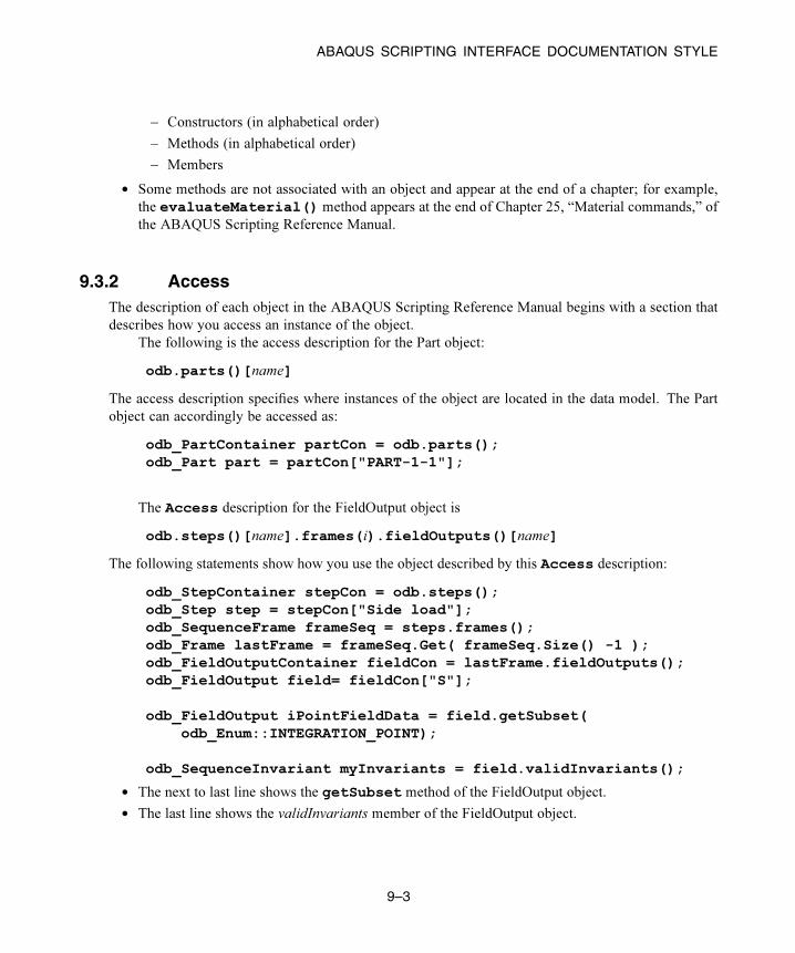
ABAQUS SCRIPTING INTERFACE DOCUMENTATION STYLE
– Constructors (in alphabetical order)
– Methods (in alphabetical order)
– Members
• Some methods are not associated with an object and appear at the end of a chapter; for example,
the evaluateMaterial() method appears at the end of Chapter 25, “Material commands,” of
the ABAQUS Scripting Reference Manual.
9.3.2 Access
The description of each object in the ABAQUS Scripting Reference Manual begins with a section that
describes how you access an instance of the object.
The following is the access description for the Part object:
odb.parts()[name]
The access description specifies where instances of the object are located in the data model. The Part
object can accordingly be accessed as:
odb_PartContainer partCon = odb.parts();odb_Part part = partCon["PART-1-1"];
The Access description for the FieldOutput object is
odb.steps()[name].frames(i).fieldOutputs()[name]
The following statements show how you use the object described by this Access description:
odb_StepContainer stepCon = odb.steps();odb_Step step = stepCon["Side load"];odb_SequenceFrame frameSeq = steps.frames();odb_Frame lastFrame = frameSeq.Get( frameSeq.Size() -1 );odb_FieldOutputContainer fieldCon = lastFrame.fieldOutputs();odb_FieldOutput field= fieldCon["S"];
odb_FieldOutput iPointFieldData = field.getSubset(odb_Enum::INTEGRATION_POINT);
odb_SequenceInvariant myInvariants = field.validInvariants();
• The next to last line shows the getSubset method of the FieldOutput object.
• The last line shows the validInvariants member of the FieldOutput object.
9–3
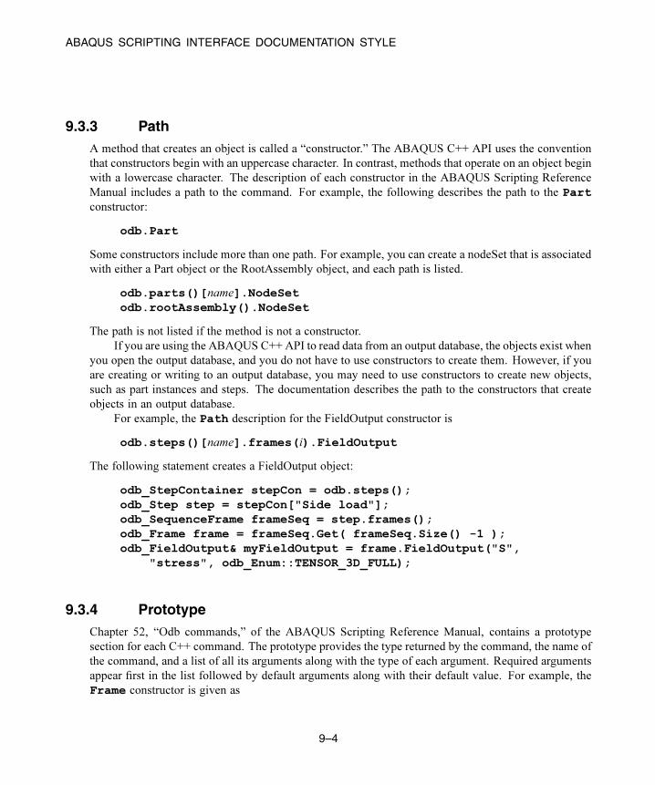
ABAQUS SCRIPTING INTERFACE DOCUMENTATION STYLE
9.3.3 Path
A method that creates an object is called a “constructor.” The ABAQUS C++ API uses the convention
that constructors begin with an uppercase character. In contrast, methods that operate on an object begin
with a lowercase character. The description of each constructor in the ABAQUS Scripting Reference
Manual includes a path to the command. For example, the following describes the path to the Partconstructor:
odb.Part
Some constructors include more than one path. For example, you can create a nodeSet that is associated
with either a Part object or the RootAssembly object, and each path is listed.
odb.parts()[name].NodeSetodb.rootAssembly().NodeSet
The path is not listed if the method is not a constructor.
If you are using the ABAQUS C++ API to read data from an output database, the objects exist when
you open the output database, and you do not have to use constructors to create them. However, if you
are creating or writing to an output database, you may need to use constructors to create new objects,
such as part instances and steps. The documentation describes the path to the constructors that create
objects in an output database.
For example, the Path description for the FieldOutput constructor is
odb.steps()[name].frames(i).FieldOutput
The following statement creates a FieldOutput object:
odb_StepContainer stepCon = odb.steps();odb_Step step = stepCon["Side load"];odb_SequenceFrame frameSeq = step.frames();odb_Frame frame = frameSeq.Get( frameSeq.Size() -1 );odb_FieldOutput& myFieldOutput = frame.FieldOutput("S",
"stress", odb_Enum::TENSOR_3D_FULL);
9.3.4 Prototype
Chapter 52, “Odb commands,” of the ABAQUS Scripting Reference Manual, contains a prototype
section for each C++ command. The prototype provides the type returned by the command, the name of
the command, and a list of all its arguments along with the type of each argument. Required arguments
appear first in the list followed by default arguments along with their default value. For example, the
Frame constructor is given as
9–4

HOW THE OBJECT MODEL FOR THE OUTPUT DATABASE RELATES TO COMMANDS
odb_Frame& Frame(int frameId, double frameValue,const odb_String& description="");
indicating that the frameId and frameValue arguments are required, that the optional description argument
has a default value of the empty string, and that the method returns a reference to the Frame object created.
9.3.5 Return value
All commands return a value. Many commands return the value void. Constructors (methods that
create an object) always return the object being created. The return value of a command can be assigned
to a variable. For example, in the following statement the Odb constructor returns an Odb object, and
the variable newOdb refers to this new object.
odb_Odb newOdb& = Odb("new", "", "", fileName);
You can use the object returned by a command in subsequent statements. The following statement uses
the output database created by the previous statement:
odb_Part& part = newOdb.Part("PART-1-1",odb_Enum::THREE_D, odb_Enum::DEFORMABLE_BODY);
If an exception is raised while a statement is executing, the command does not return a value.
9.4 How the object model for the output database relates to
commands
You need to understand the object model for the output database both to read data from it and to write
data to it. An object model describes the relationship between objects. The object model for the
ABAQUS/CAE model is described in “The ABAQUS object model,” Section 6.1.
For example, consider the object model for field output data shown in Figure 9–1. The Odb object
at the top of the figure is created when you issue the command to open or create an output database. As
you move down the object model, an OdbStep object is a member of the Odb object; similarly, a Frame
object is a member of the OdbStep object. The FieldOutput object has two members—fieldValue and
fieldLocation.
The object model translates directly to the structure of an ABAQUS C++ API command. For
example, the following command refers to a Frame object in the sequence of frames contained in an
OdbStep object:
odb.steps()["10 hz"].frames(3);
Similarly, the following command refers to the sequence of field data contained in a FieldOutput object.
odb.steps()["10 hz"].frames.Get(3).
9–5
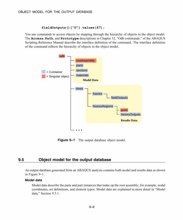
OBJECT MODEL FOR THE OUTPUT DATABASE
fieldOutputs()["U"].values(47);
You use commands to access objects by stepping through the hierarchy of objects in the object model.
The Access, Path, and Prototype descriptions in Chapter 52, “Odb commands,” of the ABAQUS
Scripting Reference Manual describe the interface definition of the command. The interface definition
of the command reflects the hierarchy of objects in the object model.
steps
= Container = Singular object
odbrootAssembly
parts
sections
Model Data
frames
historyRegions
Results Data
pointhistoryOutputs
fieldOutputs
materials
Figure 9–1 The output database object model.
9.5 Object model for the output database
An output database generated from an ABAQUS analysis contains both model and results data as shown
in Figure 9–1.
Model data
Model data describe the parts and part instances that make up the root assembly; for example, nodal
coordinates, set definitions, and element types. Model data are explained in more detail in “Model
data,” Section 9.5.1.
9–6

OBJECT MODEL FOR THE OUTPUT DATABASE
Results data
Results data describe the results of your analysis; for example, stresses, strains, and displacements.
You use output requests to configure the contents of the results data. Results data can be either field
output data or history output data; for a more detailed explanation, see “Results data,” Section 9.5.2.
Note: For a description of object models, see “An overview of the ABAQUS object model,”
Section 6.1.1.
You can find more information on the format of the output database in “Output to the output database,”
Section 4.1.3 of the ABAQUS Analysis User’s Manual.
9.5.1 Model data
Model data define the model used in the analysis; for example, the parts, materials, initial and boundary
conditions, and physical constants. More information about model data can be found in “The ABAQUS
object model,” Section 6.1, and “Defining an assembly,” Section 2.9.1 of the ABAQUS Analysis User’s
Manual.
ABAQUS does not write all the model data to the output database; for example, you cannot access
loads and interactions. Model data that are stored in the output database include parts, the root assembly,
part instances, regions, materials, sections, section assignments, and section categories, each of which is
stored as an ABAQUS C++ API object. These components of model data are described below.
Parts
Apart in the output database is a finite element idealization of an object. Parts are the building blocks
of an assembly and can be either rigid or deformable. Parts are reusable; they can be instanced
multiple times in the assembly. Parts are not analyzed directly; a part is like a blueprint for its
instances. A part is stored in an output database as a collection of nodes, elements, surfaces, and
sets.
The root assembly
The root assembly is a collection of positioned part instances. An analysis is conducted by defining
boundary conditions, constraints, interactions, and a loading history for the root assembly. The
output database object model contains only one root assembly.
Part instances
A part instance is a usage of a part within the assembly. All characteristics (such as mesh and
section definitions) defined for a part become characteristics for each instance of that part—they
are inherited by the part instances. Each part instance is positioned independently within the root
assembly.
9–7

OBJECT MODEL FOR THE OUTPUT DATABASE
Materials
Materials contain material models comprised of one or more material property definitions. The same
material models may be used repeatedly within a model; each component that uses the samematerial
model shares identical material properties. Many materials may exist within a model database, but
only the materials that are used in the assembly are copied to the output database.
Sections
Sections add the properties that are necessary to define completely the geometric and material
properties of an element. Various element types require different section types to complete their
definitions. For example, shell elements in a composite part require a section that provides a
thickness, multiple material models, and an orientation for each material model; all these pieces
combine to complete the composite shell element definition. Like materials, only those sections
that are used in the assembly are copied to the output database.
Section assignments
Section assignments link section definitions to the regions of part instances. Section assignments
in the output database maintain this association. Sections are assigned to each part in a model, and
the section assignments are propagated to each instance of that part.
Section categories
You use section categories to group the regions of the model that use the same section definitions;
for example, the regions that use a shell section with five section points. Within a section category,
you use the section points to identify the location of results; for example, you can associate section
point 1 with the top surface of a shell and section point 5 with the bottom surface.
Figure 9–2 shows the model data object model.
9.5.2 Results data
Results data describe the results of your analysis. ABAQUS organizes the analysis results in an output
database into the following components:
Steps
An ABAQUS analysis contains a sequence of one or more analysis steps. Each step is associated
with an analysis procedure.
Frames
Each step contains a sequence of frames, where each increment of the analysis that resulted in output
to the output database is called a frame. In a frequency or buckling analysis each eigenmode is stored
as a separate frame. Similarly, in a steady-state harmonic response analysis each frequency is stored
as a separate frame.
9–8

OBJECT MODEL FOR THE OUTPUT DATABASE
steps
frames
historyRegions
fieldOutputs
pointhistoryOutputs
= Container = Singular object
odb
nodeSets
elementSets
surfaces
instances
nodeSets
elementSets
surfaces
elements
nodes
rootAssembly
parts
sections
sectionPoints
Model Data
Results Data
materials
Figure 9–2 The model data object model.
Field output
Field output is intended for infrequent requests for a large portion of the model and can be used to
generate contour plots, animations, symbol plots, and displaced shape plots in the Visualization
module of ABAQUS/CAE. You can also use field output to generate an X–Y data plot. Only
complete sets of basic variables (for example, all the stress or strain components) can be requested
as field output. Field output is composed of a “cloud of data values” (e.g., stress tensors at each
integration point for all elements). Each data value has a location, type, and value. You use the
regions defined in the model data, such as an element set, to access subsets of the field output data.
Figure 9–3 shows the field output data object model within an output database.
9–9

OBJECT MODEL FOR THE OUTPUT DATABASE
steps
historyRegions
= Container = Singular object
odbrootAssembly
parts
sections
Model Data
Results Data
frames
fieldValuesfieldOutputs
materials
Figure 9–3 The field output data object model.
History output
History output is output defined for a single point or for values calculated for a portion of the model
as a whole, such as energy. History output is intended for relatively frequent output requests for
small portions of the model and can be displayed in the form of X–Y data plots in the Visualization
module of ABAQUS/CAE. Individual variables (such as a particular stress component) can be
requested.
Depending on the type of output expected, a HistoryRegion object can be defined for one of
the following:
• a node
• an integration point
• a region
• the whole model
The output from all history requests that relate to a particular point or region is then collected in
one HistoryRegion object. Figure 9–4 shows the history output data object model within an output
database.
9–10

COMPILING AND LINKING YOUR C++ SOURCE CODE
steps
frames
= Container = Singular object
odbrootAssembly
parts
data
sections
Model Data
Results Data
historyRegionspoint
historyOutputs
fieldOutputs
materials
Figure 9–4 The history output data.
9.6 Compiling and linking your C++ source code
Sample postprocessing programs to perform commonly exercised tasks are presented in separate
sections in this chapter. These and other C++ postprocessing programs must be compiled and linked
using the make parameter when running the ABAQUS execution procedure (see “Execution procedure
for ABAQUS/Make,” Section 3.2.13 of the ABAQUS Analysis User’s Manual). To link properly, the
programs cannot contain a C++ main routine. Instead, the programs must begin with a C++ function
called ABQmain.
#include <odb_API.h>
int ABQmain(int argc, char **argv){
//Insert user code herereturn 0
}
The arguments passed into the program upon execution will be passed into ABQmain as though it were
the standard C++main function. The compile and link commands used by the ABAQUS/Make procedure
9–11

ACCESSING THE C++ INTERFACE FROM AN EXISTING APPLICATION
are determined by the settings of the compile_cpp and link parameters in the ABAQUS environment
file.
9.7 Accessing the C++ interface from an existing application
This section provides information that may be helpful to users who need to access results in an output
database from an existing application. Most users should find that the ABAQUS/Make procedure is
sufficient for their postprocessing needs. Since linking and executing with dynamically linked runtime
libraries is highly system dependent, the information in this section is intended for users who have an
advanced working knowledge of compilation and linking with runtime libraries. It is important to ensure
that the compiler used to compile and link the existing application is consistent with the compilers used
to generate the ABAQUS release. The ABAQUS web site www.abaqus.com lists the name and version
of the compiler used for the ABAQUS release on each supported platform. You can find the information
under the system requirements described on the “Technical Support” pages.
The following topics are covered in this section:
• “Initializing the C++ interface,” Section 9.7.1
• “Link library location,” Section 9.7.2
• “Runtime library location,” Section 9.7.3
• “Header file location,” Section 9.7.4
9.7.1 Initializing the C++ interface
Before any calls are made to the C++ interface, the following call must be made to initialize the interface:
odb_initializeAPI();
This call is generated automatically when the ABAQUS/Make procedure is run but must be included in
any application that is not compiled and linked using the ABAQUS/Make procedure. After all calls to
the C++ interface have been completed, the interface may be deactivated by including a call to
odb_finalizeAPI();
If the finalization call is not made explicitly, the finalize routine will be called automatically when
the application exits.
9.7.2 Link library location
The libraries necessary to link applications that access the C++ interface are located in the following
directories:
9–12

ACCESSING THE C++ INTERFACE FROM AN EXISTING APPLICATION
UNIX
abaqus_dir/cae/exec/lbr
Windows
abaqus_dir\cae\exec\lbr
where abaqus_dir is the name of the directory in which ABAQUS is installed. To determine the location
of abaqus_dir at your site, type abaqus whereami at an operating system prompt.
During linking, the ABQodb library and several other libraries shipped with the ABAQUS release
are used to resolve all the functions available in the interface to the output database. The command
used by ABAQUS to link runtime libraries (for example, for user subroutines) is available through
the ABAQUS environment variable link_sl. Additional information about linking with the ABAQUS
libraries, including the names of all libraries which must be specified as part of the link command, may
be obtained by running the ABAQUS/Make procedure in verbose mode with a verbosity level of 3.
9.7.3 Runtime library location
The runtime libraries required to execute a program that accesses the C++ interface are located in the
following directories:
UNIX
abaqus_dir/cae/exec/lbr
Windows
abaqus_dir\cae\exec\lbr
where abaqus_dir is the name of the directory in which ABAQUS is installed. To determine the location
of abaqus_dir at your site, type abaqus whereami at an operating system prompt.
The correct path to the ABAQUS runtime libraries must be specified prior to starting the
user application. The runtime library path is typically set using the system environment variable
LD_LIBRARY_PATH, but the method used to set the path may vary depending on your operating
system configuration. The ABQodb library and several utility libraries resolve all the functions available
in the interface to the output database, as described in “Link library location,” Section 9.7.2. At runtime
these libraries depend on many of the underlying ABAQUS libraries. As a result, if you do not define
the correct runtime library path, your application will not run.
9.7.4 Header file location
The header files required to compile a program that accesses the C++ interface are located in the following
directories:
9–13
THE ABAQUS C++ API ARCHITECTURE
UNIX
abaqus_dir/cae/include
Windows
abaqus_dir\cae\include
where abaqus_dir is the name of the directory in which ABAQUS is installed. To determine the location
of abaqus_dir at your site, type abaqus whereami at an operating system prompt.
Only odb_API.h must be included to access the C++ interface, but the path to the header files
must be provided during compilation.
9.8 The ABAQUS C++ API architecture
This section describes the architecture of the ABAQUS C++ interface to an output database. The output
database is an object-oriented database, which means that the data are held by “objects” (C++ classes)
that have certain behavior (C++ methods). The methods of an object in the database allow access to
and manipulation of the data held by the object. The data members of an object can be either primitives
(integer, floating point, string) or other objects.
The following topics are covered:
• “Class naming convention,” Section 9.8.1
• “Constructors,” Section 9.8.2
• “Header files,” Section 9.8.3
9.8.1 Class naming convention
All class names start with odb_ to avoid possible name clashes. For example, the string class is named
odb_String.
9.8.2 Constructors
A constructor is a method that creates an object. The ABAQUS C++ API uses the following three types
of constructors:
Constructors for nonpersistent objects
Constructors for nonpersistent objects are the standard C++ constructors. For example,
odb_String partName("New_Part");
9–14

THE ABAQUS C++ API ARCHITECTURE
Constructors for persistent objects
You create a persistent object by calling a method on an existing ABAQUS C++ API object. In
ABAQUS the convention is that the constructor method name corresponds to the name of the object
created and that the first letter of the constructor name is capitalized. The object can be accessed
using the return value of the constructor call or using a lowercase version of the method name. For
example, a Frame object can be created using the following:
odb_Frame s1_writeFrame2 = step1.Frame(2, 1.3,"frame 2 of step1 at time 1.3");
The Frame object can be retrieved with the following:
odb_Frame& s1_readFrame2 = step1.frames(1);
Constructors for objects created in large quantities
For efficiency the constructors for objects that you create in large quantities, such as elements,
nodes, and field values, do not follow the capitalized constructor name rule used for persistent
objects. Nodes, elements, and field values are created using the addNodes, addElements,and addData methods, respectively. For example, you use the addNodes method to create and
retrieve nodes:
part1.addNodes(nodeLabels, coordinates, nodeSetName);const odb_SequenceNode& nodeSeq = part1.nodes();
odb_Node node1 = part1.nodes(1);
9.8.3 Header files
To use a class in a C++ program, the relevant header files must be included. The naming convention
followed is that the file name is the same as the name of the class declared in the header file. For example,
the odb_FieldValue object is declared in the file odb_FieldValue.h. The file odb_API.h includes
all the header files required to use the API. Other header files must be included to use some classes:
• To access material objects you must include the file odb_MaterialTypes.h.
• To access section objects you must include the file odb_SectionTypes.h.
9–15

UTILITY INTERFACE
9.9 Utility interface
The ABAQUS C++ API provides a set of utilities that allow a user to access certain commonly used
functionality (such as strings, sequences (lists), and repositories) quickly and easily using a set of
supported and maintained interfaces.
The following topics are covered:
• “Utility interface classes,” Section 9.9.1
• “Utility interface examples,” Section 9.9.2
9.9.1 Utility interface classes
The following interface classes are provided:
Strings
The odb_String object provides a convenient means of storing and passing strings. The odb_String
object also provides a simple interface to append and modify the data stored in the string.
Sequences
An odb_Sequence class is a container used to hold an ordered list of objects of a specific type. Data
can be appended and retrieved from the sequence.
The following odb_Sequence objects are provided to store integer, float, and enumeration data:
• odb_SequenceInt
• odb_SequenceFloat
• odb_SequenceString
• odb_SequenceInvariant
• odb_SequenceElementFace
Sequences of sequences are also available in the following forms:
• odb_SequenceSequenceFloat
• odb_SequenceSequenceSequenceFloat
• odb_SequenceSequenceInt
• odb_SequenceSequenceElementFace
The following ABAQUS objects are also stored as sequences:
• odb_SequenceNode
• odb_SequenceElement
• odb_SequenceFieldValue
• odb_SequenceFrame
9–16

UTILITY INTERFACE
• odb_SequenceSectionPoint
• odb_SequenceLoadCase
The following ABAQUS object can be collected in a sequence for utility operations:
• odb_SequenceFieldOutput
Repositories
Repositories are provided to store objects retrieved by name. Both the repositories and the content of
the repositories are created by the API; the user can only retrieve objects from repositories. Iterators
are provided to navigate the repositories.
The following ABAQUS repositories are provided:
• odb_PartRepository
• odb_FieldOutputRepository
• odb_SectionCategoryRepository
• odb_HistoryRegionRepository
• odb_SetRepository
• odb_HistoryOutputRepository
• odb_StepRepository
• odb_InstanceRepository
More detail on these interface utility objects can be found in Chapter 52, “Odb commands,” of the
ABAQUS Scripting Reference Manual.
9.9.2 Utility interface examples
The following examples demonstrate the utility interface for each of the utility interface classes
discussed:
Strings
odb_String type = stressField.baseElementTypes()[0];odb_String elementType =
odb_String("Element type is ") + type;cout << elementType << endl;
Sequences
odb_Set& mySurface = rootAssy.surfaces()["TARGET"];const odb_String instanceName = "PART-1-1";const odb_SequenceElementFace allFaces =
mySurface.faces(instanceName);odb_SequenceSequenceElementFace newFaces;
9–17

READING FROM AN OUTPUT DATABASE
int allFaces_size = allFaces.size();for (int i=0; i<allFaces_size; i++) {
const odb_SequenceElementFace fList = allFaces[i];odb_SequenceElementFace newList;int fList_size = fList.size();for (int j=0; j<fList_size; j++) {
const odb_Enum::odb_ElementFaceEnum face = fList[j];newList.append(face);
}newFaces.append(newList);
}
Repositories
odb_StepRepository stepCon = odb.steps();odb_StepRepositoryIT iter (stepCon);for (iter.first(); !iter.isDone(); iter.next()) {
cout << "step name : " << iter.currentKey() << endl;const odb_Step& step = iter.currentValue();cout << "step description : " << step.description();cout << endl;
}
9.10 Reading from an output database
The following sections describe how you use ABAQUS C++ API commands to read data from an output
database. The following topics are covered:
• “The ABAQUS/CAE Visualization module tutorial output database,” Section 9.10.1
• “Making the Odb commands available,” Section 9.10.2
• “Opening an output database,” Section 9.10.3
• “Reading model data,” Section 9.10.4
• “Reading results data,” Section 9.10.5
• “Reading field output data,” Section 9.10.6
• “Using bulk data access to an output database,” Section 9.10.7
• “Using regions to read a subset of field output data,” Section 9.10.8
• “Reading history output data,” Section 9.10.9
• “An example of reading field data from an output database,” Section 9.10.10
9–18

READING FROM AN OUTPUT DATABASE
9.10.1 The ABAQUS/CAE Visualization module tutorial output database
The following sections describe how you can access the data in an output database. Examples
are included that refer to the ABAQUS/CAE Visualization module tutorial output database,
viewer_tutorial.odb. This database is generated by the input file from Case 2 of the example
problem, “Indentation of an elastomeric foam specimen with a hemispherical punch,” Section 1.1.4
of the ABAQUS Example Problems Manual. The problem studies the behavior of a soft elastomeric
foam block indented by a heavy metal punch. The tutorial shows how you can use the Visualization
module to view the data in the output database. The tutorial describes how you can choose the variable
to display, how you can step through the steps and frames in the analysis, and how you can create X–Y
data from history output.
You are encouraged to copy the tutorial output database to a local directory and experiment with
the ABAQUS C++ API. The output database and the example scripts from this manual can be copied to
the user’s working directory using the ABAQUS fetch utility:
abaqus fetch job=name
where name.C is the name of the program or name.odb is the name of the output database (see
“Execution procedure for ABAQUS/Fetch,” Section 3.2.12 of the ABAQUS Analysis User’s Manual).
For example, use the following command to retrieve the tutorial output database:
abaqus fetch job=viewer_tutorial
9.10.2 Making the Odb commands available
To make the Odb commands available to your program, you first need to include the output database
interface classes using the following statement:
#include <odb_API.h>
To make the material and section Odb commands available to your program, you also need to include
their output database classes:
#include <odb_MaterialTypes.h>#include <odb_SectionTypes.h>
9.10.3 Opening an output database
You use the openOdbmethod to open an existing output database. For example, the following statement
opens the output database used by the ABAQUS/CAE Visualization module tutorial:
odb_Odb& odb = openOdb("viewer_tutorial.odb");
9–19
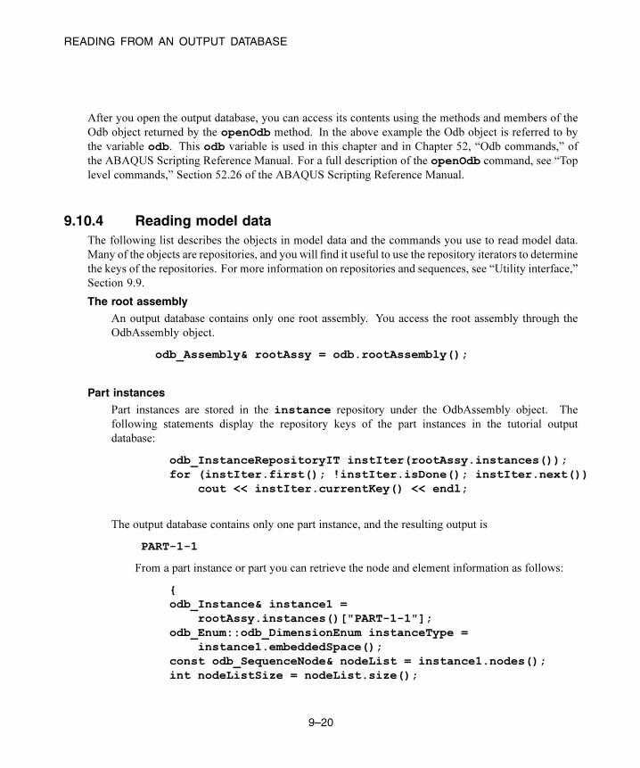
READING FROM AN OUTPUT DATABASE
After you open the output database, you can access its contents using the methods and members of the
Odb object returned by the openOdb method. In the above example the Odb object is referred to by
the variable odb. This odb variable is used in this chapter and in Chapter 52, “Odb commands,” of
the ABAQUS Scripting Reference Manual. For a full description of the openOdb command, see “Top
level commands,” Section 52.26 of the ABAQUS Scripting Reference Manual.
9.10.4 Reading model data
The following list describes the objects in model data and the commands you use to read model data.
Many of the objects are repositories, and you will find it useful to use the repository iterators to determine
the keys of the repositories. For more information on repositories and sequences, see “Utility interface,”
Section 9.9.
The root assembly
An output database contains only one root assembly. You access the root assembly through the
OdbAssembly object.
odb_Assembly& rootAssy = odb.rootAssembly();
Part instances
Part instances are stored in the instance repository under the OdbAssembly object. The
following statements display the repository keys of the part instances in the tutorial output
database:
odb_InstanceRepositoryIT instIter(rootAssy.instances());for (instIter.first(); !instIter.isDone(); instIter.next())
cout << instIter.currentKey() << endl;
The output database contains only one part instance, and the resulting output is
PART-1-1
From a part instance or part you can retrieve the node and element information as follows:
{odb_Instance& instance1 =
rootAssy.instances()["PART-1-1"];odb_Enum::odb_DimensionEnum instanceType =
instance1.embeddedSpace();const odb_SequenceNode& nodeList = instance1.nodes();int nodeListSize = nodeList.size();
9–20

READING FROM AN OUTPUT DATABASE
if (instanceType == odb_Enum::THREE_D) {for (int n=0; n<nodeListSize; n++) {
const odb_Node node = nodeList[n];int nodeLabel = node.label();const float* const coord = node.coordinates();cout << "Xcoord: " << coord[0] << " , Ycoord: "
<< coord[1] << " , Zcoord: " << coord[2] << endl;}
}else if((instanceType == odb_Enum::TWO_D_PLANAR) ||
(instanceType == odb_Enum::AXISYMMETRIC)) {for (int n=0; n<nodeListSize; n++) {
const odb_Node node = nodeList[n];int nodeLabel = node.label();const float* const coord = node.coordinates();cout << "Xcoord: " << coord[0] << " , Ycoord: "
<< coord[1] << endl;}
}
const odb_SequenceElement& elementList =instance1.elements();
int elementListSize = elementList.size();cout << "Element Connectivity Data" << endl;cout << "Element Label : constituent node labels ..."
<< endl;int numNodes = 0;for (int e=0; e<elementListSize; e++) {
const odb_Element element = elementList[e];int elementLabel = element.label();cout << elementLabel <<" : ";odb_String elementType = element.type();const int* const conn =
element.connectivity(numNodes);for (int j=0; j<numNodes; j++)
cout << " " << conn[j];cout << endl;
}}
9–21
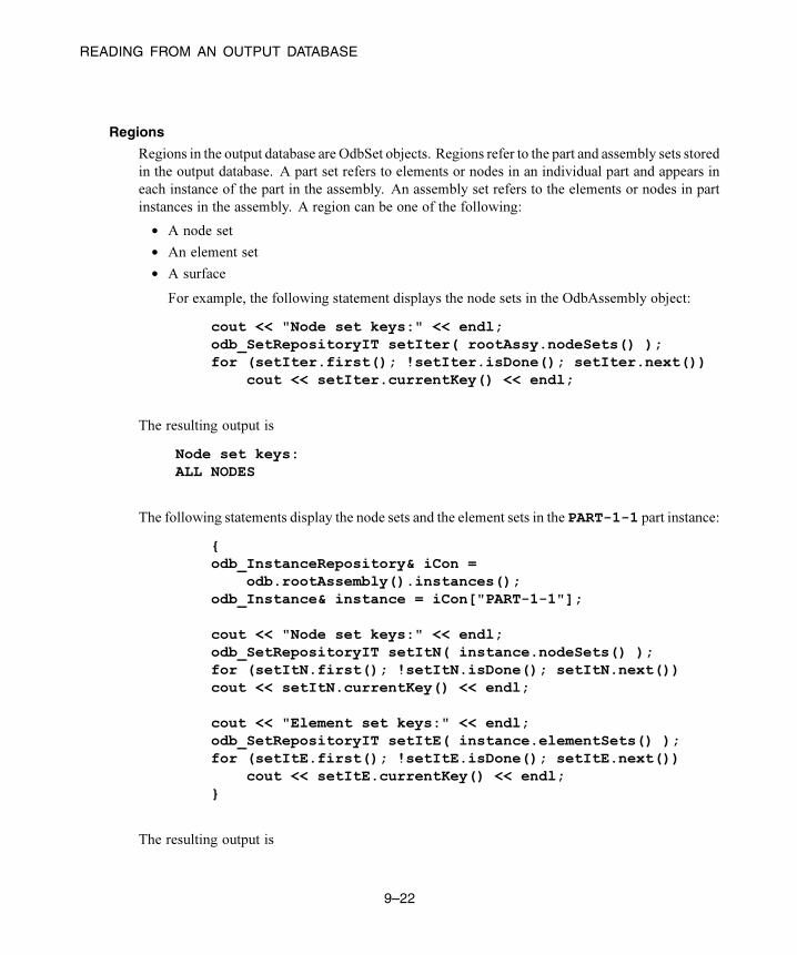
READING FROM AN OUTPUT DATABASE
Regions
Regions in the output database are OdbSet objects. Regions refer to the part and assembly sets stored
in the output database. A part set refers to elements or nodes in an individual part and appears in
each instance of the part in the assembly. An assembly set refers to the elements or nodes in part
instances in the assembly. A region can be one of the following:
• A node set
• An element set
• A surface
For example, the following statement displays the node sets in the OdbAssembly object:
cout << "Node set keys:" << endl;odb_SetRepositoryIT setIter( rootAssy.nodeSets() );for (setIter.first(); !setIter.isDone(); setIter.next())
cout << setIter.currentKey() << endl;
The resulting output is
Node set keys:ALL NODES
The following statements display the node sets and the element sets in the PART-1-1 part instance:
{odb_InstanceRepository& iCon =
odb.rootAssembly().instances();odb_Instance& instance = iCon["PART-1-1"];
cout << "Node set keys:" << endl;odb_SetRepositoryIT setItN( instance.nodeSets() );for (setItN.first(); !setItN.isDone(); setItN.next())cout << setItN.currentKey() << endl;
cout << "Element set keys:" << endl;odb_SetRepositoryIT setItE( instance.elementSets() );for (setItE.first(); !setItE.isDone(); setItE.next())
cout << setItE.currentKey() << endl;}
The resulting output is
9–22
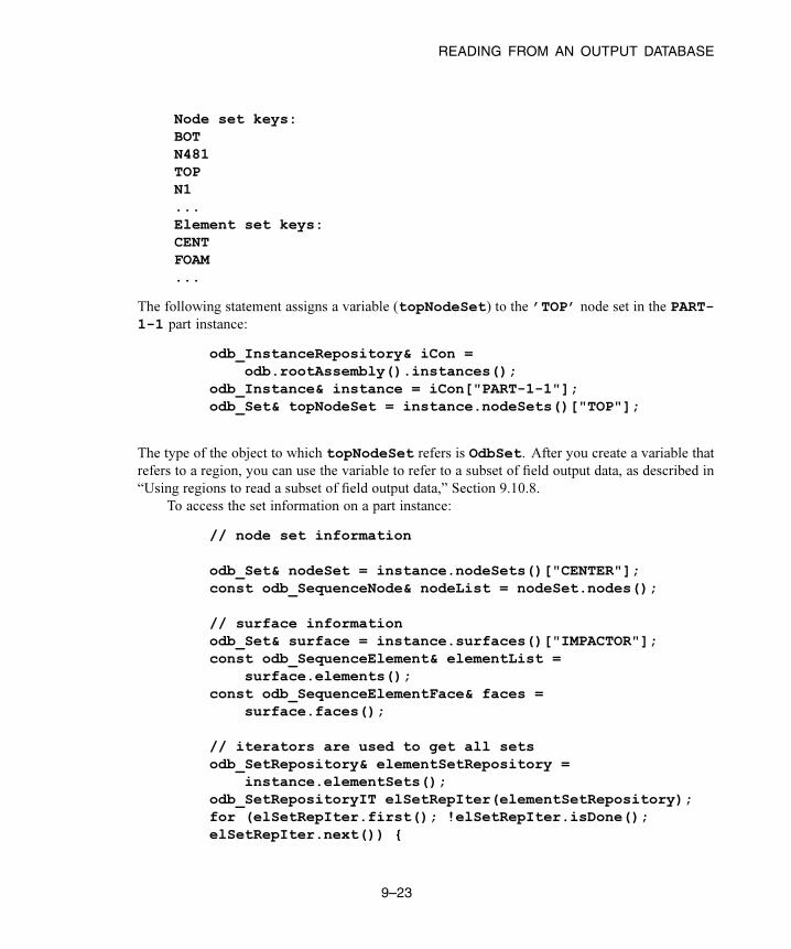
READING FROM AN OUTPUT DATABASE
Node set keys:BOTN481TOPN1...Element set keys:CENTFOAM...
The following statement assigns a variable (topNodeSet) to the ’TOP’ node set in the PART-1-1 part instance:
odb_InstanceRepository& iCon =odb.rootAssembly().instances();
odb_Instance& instance = iCon["PART-1-1"];odb_Set& topNodeSet = instance.nodeSets()["TOP"];
The type of the object to which topNodeSet refers is OdbSet. After you create a variable that
refers to a region, you can use the variable to refer to a subset of field output data, as described in
“Using regions to read a subset of field output data,” Section 9.10.8.
To access the set information on a part instance:
// node set information
odb_Set& nodeSet = instance.nodeSets()["CENTER"];const odb_SequenceNode& nodeList = nodeSet.nodes();
// surface informationodb_Set& surface = instance.surfaces()["IMPACTOR"];const odb_SequenceElement& elementList =
surface.elements();const odb_SequenceElementFace& faces =
surface.faces();
// iterators are used to get all setsodb_SetRepository& elementSetRepository =
instance.elementSets();odb_SetRepositoryIT elSetRepIter(elementSetRepository);for (elSetRepIter.first(); !elSetRepIter.isDone();elSetRepIter.next()) {
9–23

READING FROM AN OUTPUT DATABASE
odb_Set& set =elementSetRepository[elSetRepIter.currentKey()];
cout << "element set " << elSetRepIter.currentKey()<< endl;
cout << " number of elements : ";cout << set.size() << endl;
}
The set information in an assembly set is keyed by instance name and can be accessed using
the following:
// assembly surface informationodb_Set& aSurface = rootAssy.surfaces()["TARGET"];odb_SequenceString instanceNames =
aSurface.instanceNames();int totalNames = instanceNames.size();for (int name=0; name<totalNames; name++) {
const odb_String& iName = instanceNames[name];const odb_SequenceElement& els =
aSurface.elements(iName);const odb_SequenceElementFace& face =
aSurface.faces(iName);}
Materials
Materials are stored in the materials repository under the Odb object.
Extend the Material commands available to the Odb object using the following statement:
odb_MaterialApi materialApi;odb.extendApi(odb_Enum::odb_MATERIAL,materialApi);
Access the materials repository using the command:
odb_MaterialContainer& materialContainer = materialApi.materials();odb_MaterialContainerIT matIT(materialContainer);for (matIT.first(); !matIT.isDone(); matIT.next()) {
cout << "Material Name : " << matIT.currentKey() << endl;const odb_Material& myMaterial = matIT.currentValue();
To print isotropic elastic material properties in a material object:
odb_Elastic elastic = myMaterial.elastic();if (elastic.hasValue()) {
9–24

READING FROM AN OUTPUT DATABASE
if (elastic.type() == "ISOTROPIC") {cout << "isotropic elastic behavior, type = "
<< elastic.moduli() << endl;odb_String tableHeader("Youngs modulus Poisson's ratio ");if (elastic.temperatureDependency())
tableHeader.append("Temperature ");for (int i = 0, max = elastic.dependencies(); i < max; ++i)
tableHeader.append(" field # ").append(i);cout << tableHeader << endl;odb_SequenceSequenceFloat table = elastic.table();for (int r = 0, rows = table.size(); r <rows; ++r) {
const odb_SequenceFloat& data = table[r];for (int c = 0, cols = data.size(); c < cols; ++c) {
cout << data[c] << " ";}cout << endl;
}}
}
Some Material definitions have suboptions. For example, to access the smoothing type used
for biaxial test data specified for a hyperelastic material:
odb_Hyperelastic hyperelastic = myMaterial.hyperelastic();if (hyperelastic.hasValue()) {
bool testData = hyperelastic.testData();odb_BiaxialTestData biaxialTestData =
hyperelastic.biaxialTestData();odb_String smoothingType("smoothing type: ");if (biaxialTestData.hasValue()) {
odb_Union smoothing = biaxialTestData.smoothing();switch(smoothing.type()) {
case (odb_UNION_STRING):smoothingType.append(smoothing.getString());break;
case (odb_UNION_INT):smoothingType.append(smoothing.getInt());break;
case (odb_UNION_FLOAT):smoothingType.append(smoothing.getFloat());break;
case (odb_UNION_DOUBLE):
9–25

READING FROM AN OUTPUT DATABASE
smoothingType.append(smoothing.getDouble());break;
case (odb_UNION_BOOL):smoothingType.append(smoothing.getBool());break;
}cout << smoothingType << endl;
}}
Chapter 51, “Material commands,” of the ABAQUS Scripting Reference Manual, describes
the Material object commands in more detail; the odb_Union object is defined in “Union object,”
Section 55.6 of the ABAQUS Scripting Reference Manual.
Sections
Sections are stored in the sections repository under the Odb object.
Extend the Section commands available to the Odb object using the following statement:
odb_SectionApi sectionApi;odb.extendApi(odb_Enum::odb_SECTION,sectionApi);
The following statements display the repository keys of the sections in an output database:
odb_SectionContainer& sectionContainer =sectionApi.sections();
odb_SectionContainerIT scIT(sectionContainer);for (scIT.first(); !scIT.isDone(); scIT.next()) {
cout << "Section Name : " << scIT.currentKey() << endl;}
The Section object can be one of the various section types. The odb_isAmethod can be used
to determine the section type. For example, to determine whether a section is of type “homogeneous
solid section” and to print it’s thickness and associated material name:
for (scIT.first(); !scIT.isDone(); scIT.next()) {const odb_Section& mySection = scIT.currentValue();if (odb_isA(odb_HomogeneousSolidSection,mySection)) {
odb_HomogeneousSolidSection homogeneousSolidSection =odb_dynamicCast(
odb_HomogeneousSolidSection, mySection);odb_String material =
homogeneousSolidSection.material();cout << "material name = " << material << endl;float thickness = homogeneousSolidSection.thickness();
9–26

READING FROM AN OUTPUT DATABASE
cout << "thickness = " << thickness << endl;}
}
Similarily, to access the beam profile repository:
odb_ProfileContainer profileContainer =sectionApi.profiles();
int numProfiles = sectionApi.numProfiles();cout << "Total Number of profiles in the ODB: "
<< numProfiles << endl;
The Profile object can be one of the various profile types. The odb_isA method can be used
to determine the profile type. For example, to output the radius of all circular profiles in the odb:
odb_ProfileContainerIT pcIT(profileContainer);for (pcIT.first(); !pcIT.isDone(); pcIT.next()) {
const odb_Profile& myProfile = pcIT.currentValue();if (odb_isA(odb_CircularProfile,myProfile)) {
odb_CircularProfile circularProfile =odb_dynamicCast( odb_CircularProfile, myProfile );
cout << "profile name = " << myProfile.name()<< " radius = " << circularProfile.r();
}}
Section assignments
Section assignments are stored in the sectionAssignments repository under the OdbAssembly
object.
All elements in an ABAQUS analysis need to be associated with section and material
properties. Section assignments provide the relationship between elements in a part instance and
their section properties. The section properties include the associated material name. To access the
sectionAssignments repository from the PartInstance object:
odb_InstanceRepository& instanceRepository =odb.rootAssembly().instances();
odb_InstanceRepositoryIT instIT(instanceRepository);for (instIT.first(); !instIT.isDone(); instIT.next()) {
const odb_Instance& instance = instIT.currentValue();odb_SequenceSectionAssignment sectionAssignmentSeq =
instance.sectionAssignments();int sects = sectionAssignmentSeq.size();cout << "Instance : " << instance.name() << endl;for (int s = 0; s < sects; ++s) {
9–27

READING FROM AN OUTPUT DATABASE
odb_SectionAssignment sa = sectionAssignmentSeq[s];odb_Section section = sa.section();
cout << " Section : " << section.name() << endl;odb_Set set = sa.region();const odb_SequenceElement& elements = set.elements();int size = elements.size();
cout << " Elements associated with this section : "<< endl;
for (int e = 0; e< size; ++e)cout << elements[e].label() << endl;
}}
9.10.5 Reading results data
The following list describes the objects in results data and the commands you use to read results data. As
with model data you will find it useful to use the repository iterators to determine the keys of the results
data repositories.
Steps
Steps are stored in the steps repository under the Odb object. The key to the steps repository
is the name of the step. The following statements print out the keys of each step in the repository:
odb_StepRepositoryIT stepIter( odb.steps() );for (stepIter.first(); !stepIter.isDone();stepIter.next())
cout << stepIter.currentKey() << endl;
The resulting output is
Step-1Step-2Step-3
Frames
Each step contains a sequence of frames, where each increment of the analysis (or each mode in an
eigenvalue analysis) that resulted in output to the output database is called a frame. The following
statement assigns a variable to the last frame in the first step:
odb_Step& step = odb.steps()["Step-1"];odb_SequenceFrame& allFramesInStep = step.frames();int numFrames = allFramesInStep.size();
9–28
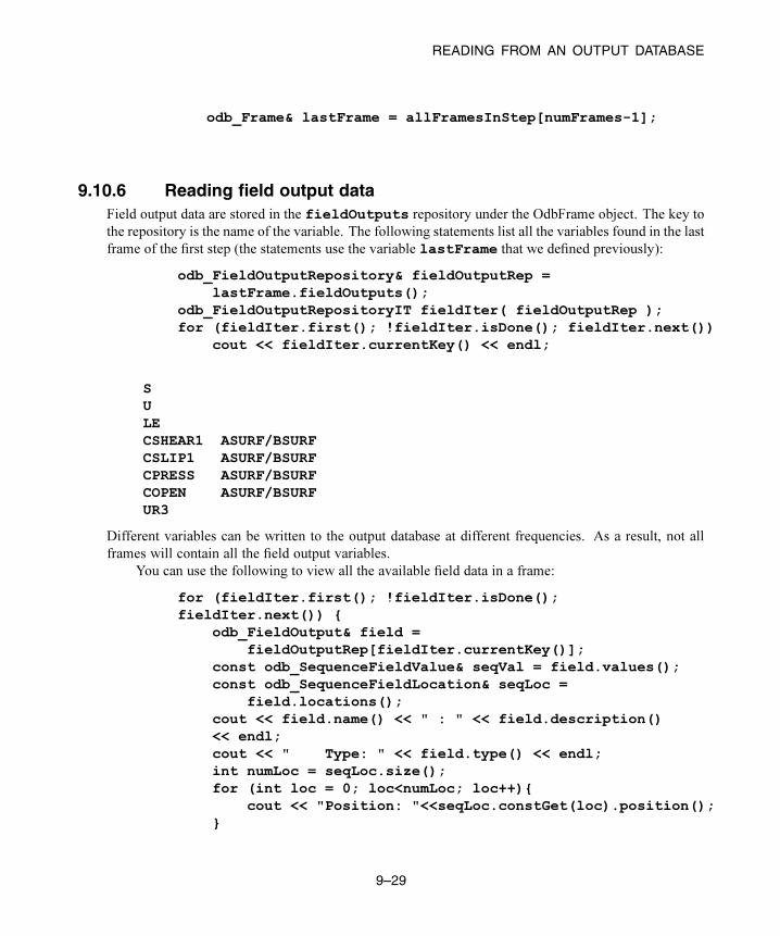
READING FROM AN OUTPUT DATABASE
odb_Frame& lastFrame = allFramesInStep[numFrames-1];
9.10.6 Reading field output data
Field output data are stored in the fieldOutputs repository under the OdbFrame object. The key to
the repository is the name of the variable. The following statements list all the variables found in the last
frame of the first step (the statements use the variable lastFrame that we defined previously):
odb_FieldOutputRepository& fieldOutputRep =lastFrame.fieldOutputs();
odb_FieldOutputRepositoryIT fieldIter( fieldOutputRep );for (fieldIter.first(); !fieldIter.isDone(); fieldIter.next())
cout << fieldIter.currentKey() << endl;
SULECSHEAR1 ASURF/BSURFCSLIP1 ASURF/BSURFCPRESS ASURF/BSURFCOPEN ASURF/BSURFUR3
Different variables can be written to the output database at different frequencies. As a result, not all
frames will contain all the field output variables.
You can use the following to view all the available field data in a frame:
for (fieldIter.first(); !fieldIter.isDone();fieldIter.next()) {
odb_FieldOutput& field =fieldOutputRep[fieldIter.currentKey()];
const odb_SequenceFieldValue& seqVal = field.values();const odb_SequenceFieldLocation& seqLoc =
field.locations();cout << field.name() << " : " << field.description()<< endl;cout << " Type: " << field.type() << endl;int numLoc = seqLoc.size();for (int loc = 0; loc<numLoc; loc++){
cout << "Position: "<<seqLoc.constGet(loc).position();}
9–29

READING FROM AN OUTPUT DATABASE
cout << endl;}
The resulting print output lists all the field output variables in a particular frame, along with their type
and position.
S : Stress componentsType: 7Number of fieldValues : 135Number of locations : 1
U : Spatial displacementType: 3Number of fieldValues : 161Number of locations : 1
In turn, a FieldOutput object has a method values that returns a reference to a sequence of
FieldValue objects that contain data. Each FieldValue object in the sequence corresponds to a particular
location in the model. You can obtain the data corresponding to each FieldValue object using the datamethod, which returns a pointer to an array that contains the results at the current location. For example,
const odb_SequenceFieldValue& displacements =lastFrame.fieldOutputs()["U"].values();
int numValues = displacements.size();int numComp = 0;for (int i=0; i<numValues; i++) {
const odb_FieldValue val = displacements[i];cout << "Node = " << val.nodeLabel();const float* const U = val.data(numComp);cout << ", U = ";for (int comp=0;comp<numComp;comp++)
cout << U[comp] << " ";cout << endl;
}
The resulting output is
Node = 1 U[x] = 0.0000, U[y] = -76.4580Node = 3 U[x] = -0.0000, U[y] = -64.6314Node = 5 U[x] = 0.0000, U[y] = -52.0814Node = 7 U[x] = -0.0000, U[y] = -39.6389Node = 9 U[x] = -0.0000, U[y] = -28.7779Node = 11 U[x] = -0.0000, U[y] = -20.3237...
9–30

READING FROM AN OUTPUT DATABASE
The data in the FieldValue object depend on the field output variable, which is displacement in the above
example. In the example above the field output for displacements was of type NODAL and there is a
FieldValue object for the output at each node. In this case the data method returns a pointer to an array
containing the displacements at the node. For INTEGRATION_POINT data each integration point in an
element will correspond to a different FieldValue object, and the data method will return a pointer to an
array containing the element results data at that particular integration point.
Note: Access to field data using the FieldValue object will be deprecated in future releases of the C++
version of the ABAQUS Scripting Interface because of the improved performance of the bulk data access
method. For more information, see “FieldBulkData object,” Section 52.2 of the ABAQUS Scripting
Reference Manual, and “Using bulk data access to an output database,” Section 9.10.7.
9.10.7 Using bulk data access to an output database
If you need to access all the data in a field from an output database, you can use the bulkDataBlocksmethod of the FieldOutput object to read the data in bulk form. The bulkDataBlocksmethod returns
a reference to a sequence of FieldBulkData objects, each of which contains the entire output for a class
of nodes or elements, blocked together into an array.
The data method of the FieldBulkData object returns an array of data corresponding to the output
for the entire class of elements or nodes. The length and width methods of theFieldBulkData object
return the number of output locations and the number of components at each output location, respectively.
For example,
odb_FieldOutput& disp = lastFrame.fieldOutputs()["U"];const odb_SequenceFieldBulkData& seqDispBulkData =
disp.bulkDataBlocks();int numDispBlocks = seqDispBulkData.size();for (int iblock=0; iblock<numDispBlocks; iblock++) {
const odb_FieldBulkData& bulkData =seqDispBulkData[iblock];
int numNodes = bulkData.length();int numComp = bulkData.width();float* data = bulkData.data();int* nodeLabels = bulkData.nodeLabels();for (int node=0,pos=0; node<numNodes; node++) {
int nodeLabel = nodeLabels[node];cout << "Node = " << nodeLabel;
cout << " U = ";for (int comp=0;comp<numComp;comp++)
cout << data[pos++] << " ";cout << endl;
}
9–31

READING FROM AN OUTPUT DATABASE
}
The numberOfElements method returns the number of elements in a block. When you
are accessing the results for elements, the numberOfElements method is useful in determining
the number of output locations per element. For example, when you are accessing element data at
integration points, you may need to determine the number of integration points per element. You can
determine the number of integration points per element by dividing the length of the block, which is the
total number of output locations, by the number of elements in the block. For example,
odb_FieldOutput& stress = lastFrame.fieldOutputs()["S"];const odb_SequenceFieldBulkData& seqStressBulkData =
stress.bulkDataBlocks();int numStressBlocks = seqStressBulkData.size();for (int jblock=0; jblock<numStressBlocks; jblock++) {
const odb_FieldBulkData& bulkData =seqStressBulkData[jblock];
int numValues = bulkData.length();int numComp = bulkData.width();float* data = bulkData.data();int nElems = bulkData.numberOfElements();int numIP = numValues/nElems;int* elementLabels = bulkData.elementLabels();int* integrationPoints = bulkData.integrationPoints();const odb_SectionPoint& myBulkSectionPoint =
bulkData.sectionPoint();int sectPoint = myBulkSectionPoint.number();if (sectPoint)
cout << "Section Point: " << sectPoint << endl;cout << "Base Element type: "
<< bulkData.baseElementType() << endl;for (int elem = 0, ipPosition=0, dataPosition=0;elem<nElems; elem++) {
cout << "El label: " << elementLabels[elem] << endl;for (int ip = 0; ip<numIP; ip++) {
cout << "Int. Point: "<< integrationPoints[ipPosition++] << endl;cout << "S = ";for (int comp = 0; comp<numComp; comp++)
cout << " " << data[dataPosition++] << " ";cout << endl;
}
9–32

READING FROM AN OUTPUT DATABASE
}}
For more information, see “FieldBulkData object,” Section 52.2 of the ABAQUS Scripting Reference
Manual.
The bulkDataBlocks method is an alternative to the values method of a FieldOutput object,
described in “Reading field output data,” Section 9.10.6. The values method of a FieldOutput object
returns a reference to a sequence of FieldValue objects that contain data. Each FieldValue object in the
sequence provides data for a unique location in the model.
Performance can be increased with the bulk data interface because the field data stored in a bulk
data block are made available in a single array of floating point numbers. If you access the same data
in nonbulk form, you must loop over a sequence of FieldValue objects and then access the data for each
location separately. Traversing an array can prove to be significantly faster than traversing a sequence of
objects and extracting data stored within the objects. As a result, accessing the data in an output database
using the bulk data interface can be significantly faster than the nonbulk form.
If you do not need to access large amounts of data, you may get better performance with the nonbulk
access method. This is especially true if the number of output locations you are accessing is smaller than
the number of elements in a class. Similarly, the nonbulk access method may be faster if the number of
nodes you are accessing is smaller than the number of nodes in an instance. The nonbulk access method
is also better suited for random access to an output database, where successive output locations to be
accessed may lie in completely different blocks.
9.10.8 Using regions to read a subset of field output data
After you have created an OdbSet object using model data, you can use the getSubsetmethod to read
only the data corresponding to that region. Typically, you will be reading data from a region that refers to
a node set or an element set. For example, the following statements create a variable called center that
refers to the node set PUNCH at the center of the hemispherical punch. In a previous section you created
the displacement variable that refers to the displacement of the entire model in the final frame of the
first step. Now you use the getSubset command to get the displacement for only the center region.
odb_Set& center = instance.nodeSets()["PUNCH"];odb_FieldOutput& fieldU = lastFrame.fieldOutputs()["U"];odb_FieldOutput centerDisp = fieldU.getSubset(center);const odb_SequenceFieldValue& centerValues =
centerDisp.values();const odb_FieldValue val = centerValues.value(0);const float* const data = val.data(numComp);cout << " Node: " << val.nodeLabel() << endl;cout << " U = ";for (int comp=0;comp<numComp;comp++)
9–33

READING FROM AN OUTPUT DATABASE
cout << data[comp] << " ";cout << endl;
The resulting output is
Node: 1000U = 0.0000 -76.4555
The arguments to getSubset are a region, an element type, a position, or section point data. The
following is a second example that uses an element set to define the region and generates formatted
output for the stress at integration points for CAX4 elements from the element set "CENT":
odb_Set& topCenter = instance.elementSets()["CENT"];odb_Step& step2 = odb.steps()["Step-2"];odb_String CAX4 = "CAX4";odb_FieldOutput& stressField =
step2.frames(3).fieldOutputs()["S"];odb_FieldOutput fieldCAX4 = stressField.getSubset(CAX4);odb_FieldOutput fieldIP =
fieldCAX4.getSubset(odb_Enum::INTEGRATION_POINT);odb_FieldOutput fieldTopCenter = fieldIP.getSubset(topCenter);const odb_SequenceFieldValue& vals = fieldTopCenter.values();int valSize = vals.size();int dSize = 0;for (int l=0; l<valSize; l++) {
const odb_FieldValue val = vals[l];cout << "Element label = " << val.elementLabel();cout << " Integration Point = " << val.integrationPoint();cout << endl;const float* const data = val.data(dSize);
cout << " S : ";for (int k=0; k < dSize; k++) {
cout << data[k] << " ";}cout << endl;
}
The resulting output is
Element label = 1 Integration Point = 1S : 0.01230 -0.05658 0.00892 -0.00015Element label = 1 Integration Point = 2
9–34
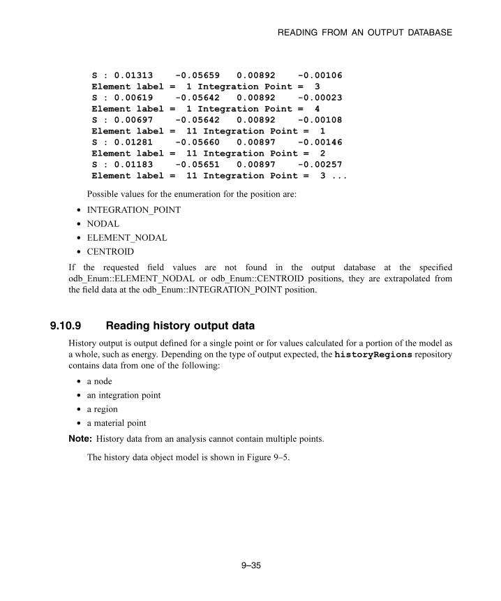
READING FROM AN OUTPUT DATABASE
S : 0.01313 -0.05659 0.00892 -0.00106Element label = 1 Integration Point = 3S : 0.00619 -0.05642 0.00892 -0.00023Element label = 1 Integration Point = 4S : 0.00697 -0.05642 0.00892 -0.00108Element label = 11 Integration Point = 1S : 0.01281 -0.05660 0.00897 -0.00146Element label = 11 Integration Point = 2S : 0.01183 -0.05651 0.00897 -0.00257Element label = 11 Integration Point = 3 ...
Possible values for the enumeration for the position are:
• INTEGRATION_POINT
• NODAL
• ELEMENT_NODAL
• CENTROID
If the requested field values are not found in the output database at the specified
odb_Enum::ELEMENT_NODAL or odb_Enum::CENTROID positions, they are extrapolated from
the field data at the odb_Enum::INTEGRATION_POINT position.
9.10.9 Reading history output data
History output is output defined for a single point or for values calculated for a portion of the model as
a whole, such as energy. Depending on the type of output expected, the historyRegions repository
contains data from one of the following:
• a node
• an integration point
• a region
• a material point
Note: History data from an analysis cannot contain multiple points.
The history data object model is shown in Figure 9–5.
9–35

READING FROM AN OUTPUT DATABASE
steps
frames
= Container = Singular object
odbrootAssembly
parts
data
sections
Model Data
Results Data
historyRegionspoint
historyOutputs
fieldOutputs
materials
Figure 9–5 The history data object model.
In contrast to field output, which is associated with a frame, history output is associated with a step.
History output data are stored in the historyRegions repository under an OdbStep object. ABAQUS
creates keys to the historyRegions repository that describe the region; for example,
• ’Node PART-1-1.1000’
• ’Element PART-1-1.2 Int Point 1’
• ’Assembly rootAssembly’
The output from all history requests that relate to a specified point is collected in one HistoryRegion
object. A HistoryRegion object contains multiple HistoryOutput objects. Each HistoryOutput object, in
turn, contains a sequence of (frameValue, value) sequences. In a time domain analysis (domain=TIME)
the sequence is a tuple of (stepTime, value). In a frequency domain analysis (domain=FREQUENCY) the
sequence is a tuple of (frequency, value). In a modal domain analysis (domain=MODAL) the sequence
is a tuple of (mode, value).
In the analysis that generated the ABAQUS/CAE Visualization module tutorial output database, the
user asked for the following history output:
At the rigid body reference point (Node 1000)
• U
• V
• A
9–36

READING FROM AN OUTPUT DATABASE
At the corner element
• MISES
• LE22
• S22
The history output data can be retrieved from the HistoryRegion objects in the output database. The
tutorial output database contains HistoryRegion objects that relate to the rigid body reference point and
the integration points of the corner element as follows:
• ’Node PART-1-1.1000’
• ’Element PART-1-1.1 Int Point 1’
• ’Element PART-1-1.1 Int Point 2’
• ’Element PART-1-1.1 Int Point 3’
• ’Element PART-1-1.1 Int Point 4’
The following statements read the tutorial output database and write the U2 history data from the second
step to an ASCII file that can be plotted by ABAQUS/CAE:
odb_Step& step = odb.steps()["Step-2"];odb_Instance& instance =
odb.rootAssembly().instances()["PART-1-1"];odb_Set& nSet = instance.nodeSets()["PUNCH"];const odb_Node node = nSet.nodes().constGet(0);odb_HistoryPoint hPoint(node);odb_HistoryRegion& histRegion =
step.getHistoryRegion(hPoint);odb_HistoryOutputRepository& hoCon =
histRegion.historyOutputs();odb_HistoryOutput& histOutU2 = hoCon["U2"];odb_SequenceSequenceFloat data = histOutU2.data();int numHDat = data.size();for (int i=0; i<numHDat; i++) {
odb_SequenceFloat pair = data[i];cout << pair.constGet(0) << " "<< pair.constGet(1) << endl;
}
The output in this example is a sequence of tuples containing the frame time and the displacement value.
The example uses nodal history data output. If the analysis requested history output from an element, the
output database would contain one HistoryRegion object and one HistoryPoint object for each integration
point.
9–37

READING FROM AN OUTPUT DATABASE
9.10.10 An example of reading field data from an output database
The following program illustrates how you readmodel data and field output data from the output database
used by the ABAQUS/CAE Visualization module tutorial output database.
Import the required modules:
#include <iostream.h>#include <odb_API.h>
Open the output database used by the tutorial.
odb_Odb& odb = openOdb("viewer_tutorial.odb");
Create a variable that refers to the last frame of the first step.
odb_Step& step = odb.steps()["Step-1"];odb_SequenceFrame& allFramesInStep = step.frames();int numFrames = allFramesInStep.size();odb_Frame& lastFrame = allFramesInStep[numFrames-1];
Create a variable that refers to the displacement ’U’ in the last frame of the first step.
odb_FieldOutput& displacements =lastFrame.fieldOutputs().get("U");
Create a variable that refers to the node set ’PUNCH’ in the part instance’PART-1–1’ :
odb_Instance& instance =odb.rootAssembly().instances()["PART-1-1"];
odb_Set& nodeSet =instance.nodeSets["PUNCH"];
Create a variable that refers to the displacement of the node set in the last frame of the first step:
odb_FieldOutput myDisplacements =displacements.getSubset(nodeSet);
Finally, print some field output data from each node in the node set (a single node in this example).
const odb_FieldValue val = myDisplacements.values()[0];const float* const data = val.data(numComp);cout << " Node: " << val.nodeLabel() << endl;cout << " U = ";for (int comp=0;comp<numComp;comp++)
9–38

WRITING TO AN OUTPUT DATABASE
cout << data[comp] << " ";cout << endl;cout << " Magnitude = " << val.magnitude();
The resulting output is
Node : 1000U = 0.0000 , -76.4554Magnitude = 76.4554
9.11 Writing to an output database
You can write your own data to an output database, and you can use ABAQUS/CAE to view the data.
Writing to an output database is very similar to reading from an output database. When you open an
existing database, the Odb object contains all the objects found in the output database, such as instances,
steps, and field output data. In contrast, when you are writing to a new output database, these objects do
not exist. As a result you must use a constructor to create the objects. For example, you use the Partconstructor to create a Part object, the Instance constructor to create an OdbInstance object, and the
Step constructor to create an OdbStep object.
After you create an object, you use methods of the objects to enter or modify the data associated
with the object. For example, if you are creating an output database, you first create an Odb object.
You then use the Part constructor to create a part. After creating the part, you use the addNodes and
addElements methods of the Part object to add nodes and elements, respectively. Similarly, you use
the addData method of the FieldOutput object to add field output data to the output database. After
creating an output database, you should use the save method on the Odb object to save the output
database.
The example program in “Creating an output database,” Section 9.15.2, also illustrates how you can
write to an output database.
The following topics are covered:
• “Creating a new output database,” Section 9.11.1
• “Writing model data,” Section 9.11.2
• “Writing results data,” Section 9.11.3
• “Writing field output data,” Section 9.11.4
• “Default display properties,” Section 9.11.5
• “Writing history output data,” Section 9.11.6
9.11.1 Creating a new output database
You use the Odb constructor to create a new, empty Odb object.
9–39

WRITING TO AN OUTPUT DATABASE
odb_Odb& odb = Odb("myData","derived data","test problem", "testWrite.odb");
For a full description of the Odb command, see “Odb,” Section 52.1.1 of the ABAQUS Scripting
Reference Manual. ABAQUS creates the RootAssembly object when you create or open an output
database.
You use the save method to save the output database.
odb.save();
For a full description of the save command, see “save,” Section 52.1.4 of the ABAQUS Scripting
Reference Manual.
9.11.2 Writing model data
To define the geometry of your model, you first create the parts that are used by the model and then you
add nodes and elements to the parts. You then define the assembly by creating instances of the parts. If
the output database already contains results data, you should not change the geometry of the model. This
is to ensure that the results remain synchronized with the model.
Part
If the part was created by ABAQUS/CAE, the description of the native ABAQUS/CAE geometry
is stored in the model database, but it is not stored in the output database. A part is stored in
an output database as a collection of nodes, elements, surfaces, and sets. You use the Partconstructor to add a part to the Odb object. You can specify the type of the part; however, only
DEFORMABLE_BODY is currently supported. For example,
odb_Part& part1 = odb.Part("part-1",odb_Enum::THREE_D, odb_Enum::DEFORMABLE_BODY);
For a full description of the Part constructor, see “OdbPart object,” Section 52.19 of the ABAQUS
Scripting Reference Manual. The new Part object is empty and does not contain geometry. After
you create the Part object, you then add nodes and elements.
You use the addNodes method to add nodes by defining node labels and coordinates. You
can also define an optional node set. For example,
odb_SequenceInt nodeLabels;nodeLabels.append(1);nodeLabels.append(2);nodeLabels.append(3);nodeLabels.append(5);
9–40
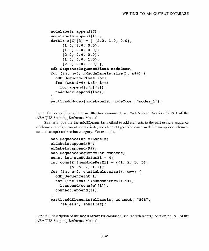
WRITING TO AN OUTPUT DATABASE
nodeLabels.append(7);nodeLabels.append(11);double c[6][3] = { {2.0, 1.0, 0.0},
{1.0, 1.0, 0.0},{1.0, 0.0, 0.0},{2.0, 0.0, 0.0},{1.0, 0.0, 1.0},{2.0, 0.0, 1.0} };
odb_SequenceSequenceFloat nodeCoor;for (int n=0; n<nodeLabels.size(); n++) {
odb_SequenceFloat loc;for (int i=0; i<3; i++)
loc.append(c[n][i]);nodeCoor.append(loc);
}part1.addNodes(nodeLabels, nodeCoor, "nodes_1");
For a full description of the addNodes command, see “addNodes,” Section 52.19.3 of the
ABAQUS Scripting Reference Manual.
Similarly, you use the addElements method to add elements to the part using a sequence
of element labels, element connectivity, and element type. You can also define an optional element
set and an optional section category. For example,
odb_SequenceInt elLabels;elLabels.append(9);elLabels.append(99);odb_SequenceSequenceInt connect;const int numNodePerEl = 4;int conn[2][numNodePerEl] = {{1, 2, 3, 5},
{5, 3, 7, 11}};for (int e=0; e<elLabels.size(); e++) {
odb_SequenceInt l;for (int i=0; i<numNodePerEl; i++)
l.append(conn[e][i]);connect.append(l);
}part1.addElements(elLabels, connect, "S4R",
"s4_els", shellCat);
For a full description of the addElements command, see “addElements,” Section 52.19.2 of the
ABAQUS Scripting Reference Manual.
9–41

WRITING TO AN OUTPUT DATABASE
The RootAssembly object
The root assembly is created when you create the output database. You access the RootAssembly
object using the same syntax as that used for reading from an output database.
odb_Assembly& rootAssy = odb.rootAssembly();
You can create both instances and regions on the RootAssembly object.
Part instances
You use the Instance constructor to create part instances of the parts you have already defined
using the Part constructor. For example,
odb_Instance& instanceA =odb.rootAssembly().Instance("part-1-1", part1);
You can also supply an optional local coordinate system that specifies the rotation and translation
of the part instance. You can add nodes and elements only to a part; you cannot add elements
and nodes to a part instance. As a result, you should create the nodes and elements that define the
geometry of a part before you instance the part. For a full description of the Instance command,
see “OdbInstance object,” Section 52.15 of the ABAQUS Scripting Reference Manual.
Regions
Region commands are used to create sets from element labels, node labels, and element faces. You
can create a set on a part, part instance, or the root assembly. Node and element labels are unique
within an instance but not within the assembly. As a result, a set on the root assembly requires
the names of the part instances associated with the nodes and elements. You can also use region
commands to create surfaces.
For example,
// An ElementSet on an instanceodb_SequenceInt eLabelsA(2);eLabelsA.append(9);eLabelsA.append(99);instanceA.ElementSet("elSetA", eLabelsA);
// A NodeSet on the rootAssembly
odb_SequenceSequenceInt nodeLabelsRA;odb_SequenceString namesRA;namesRA.append("part-1-1");odb_SequenceInt nodeLabelsRA_A;
9–42

WRITING TO AN OUTPUT DATABASE
nodeLabelsRA_A.append(5);nodeLabelsRA_A.append(11);nodeLabelsRA.append(nodeLabelsRA_A);const odb_Set& nSetRA = rootAssy.NodeSet("nodeSetRA",
namesRA, nodeLabelsRA);
Materials
You use the Material object to list material properties. Material objects are members of the Odb
object.
Materials are stored in the materials repository under the Odb object.
Extend the Material commands available to the Odb object using the following statement:
odb_MaterialApi materialApi;odb.extendApi(odb_Enum::odb_MATERIAL,materialApi);
To create an isotropic elastic material, with a Young’s modulus of 12000.0 and an effective
Poisson’s ratio of 0.3 in the output database:
odb_String materialName("Elastic Material");odb_Material& material = materialApi.Material(materialName);odb_SequenceSequenceFloat myTable;odb_SequenceFloat myData;myData.append(12000.0); myData.append(0.3);myTable.append(myData);odb_String type("ISOTROPIC");material.Elastic(myTable,type);
For more information, see Chapter 51, “Material commands,” of the ABAQUS Scripting
Reference Manual.
Sections
You use the Section object to create sections and profiles. Section objects are members of the Odb
object.
Sections are stored in the sections repository under the Odb object.
Extend the API commands available to the Odb object using the following statement:
odb_SectionApi sectionApi;odb.extendApi(odb_Enum::odb_SECTION,
sectionApi);
The following code creates a homogeneous solid section object. A Material object must be
present before creating a Section object. An exception is thrown if the material does not exist.
odb_String sectionName("Homogeneous Solid Section");
9–43

WRITING TO AN OUTPUT DATABASE
float thickness = 2.0;odb_HomogeneousSolidSection& mySection =
sectionApi.HomogeneousSolidSection( sectionName,materialName,thickness);
To create a circular beam profile object in the output database:
odb_String profileName("Circular Profile");float radius = 10.00;sectionApi.CircularProfile(profileName, radius);
Section assignments
You use the SectionAssignment object to assign sections and their associated material properties
to regions of the model. SectionAssignment objects are members of the Odb object. For a full
description of the assignSection method, see “assignSection,” Section 52.15.7 of the ABAQUS
Scripting Reference Manual.
All Elements in an ABAQUS analysis need to be associated with section and material
properties. Section assignments provide the relationship between elements in an Instance object
and their section properties. The section properties include the associated material name. To create
an element set and assign a section:
odb_SequenceInt setLabels;setLabels.append(1);setLabels.append(2);elsetName = "Material 1";odb_Set& elset = instance.ElementSet(elsetName,setLabels);// section assignment on instanceinstance.assignSection(elset,section);
9.11.3 Writing results data
To write results data to the output database, you first create the Step objects that correspond to each step
of the analysis. If you are writing field output data, you also create the Frame objects that will contain
the field data. History output data are associated with Step objects.
Steps
You use the Step constructor to create a results step for time, frequency, or modal domain results.
For example,
odb_Step& step1 = odb.Step("s1","Perturbation Step", odb_Enum::TIME);
9–44

WRITING TO AN OUTPUT DATABASE
odb_Step& step2 = odb.Step("sT","Time domain analysis", odb_Enum::TIME, 1.0);
odb_Step& step3 = odb.Step("sF","Frequency analysis", odb_Enum::FREQUENCY, 123.4);
The Step constructor has an optional previousStepName argument that specifies the step after
which this step must be inserted in the steps repository. For a full description of the Stepcommand, see “Step,” Section 52.21.1 of the ABAQUS Scripting Reference Manual.
Frames
You use the Frame constructor to create a frame for field output. For example,
odb_Frame frameOne = step2.Frame(1, 0.3, "first frame");
For a full description of the Frame command, see “Frame,” Section 52.14.3 of the ABAQUS
Scripting Reference Manual.
9.11.4 Writing field output data
A FieldOutput object contains a “cloud of data values” (e.g., stress tensors at each integration point for
all elements). Each data value has a location, type, and value. You add field output data to a Frame object
by first creating a FieldOutput object using the FieldOutput constructor and then adding data to the
FieldOutput object using the addData method. For example,
// vectorodb_SequenceString vectorCompLabels;vectorCompLabels.append("1");vectorCompLabels.append("2");vectorCompLabels.append("3");odb_SequenceInvariant vectorInvar;vectorInvar.append(odb_Enum::MAGNITUDE);odb_FieldOutput& vectorField = frameOne.FieldOutput("U",
"displacement vector",odb_Enum::VECTOR,
vectorCompLabels, vectorInvar);
odb_SequenceInt labels2;labels2.append(3);labels2.append(5);odb_SequenceSequenceFloat vecDat;odb_SequenceFloat v1;
9–45

WRITING TO AN OUTPUT DATABASE
v1.append(1.1); v1.append(1.2); v1.append(1.3);vecDat.append(v1);odb_SequenceFloat v2;v2.append(2.1); v2.append(2.2); v2.append(2.3);vecDat.append(v2);
vectorField.addData(odb_Enum::NODAL, instanceA,labels2, vecDat);
For a full description of the FieldOutput constructor, see “FieldOutput,” Section 52.4.1 of the
ABAQUS Scripting Reference Manual.
The type argument to the FieldOutput constructor describes the type of the data—tensor, vector,
or scalar. The properties of the different tensor types are:
Full tensor
A tensor that has six components and three principal values. Full three-dimensional rotation of the
tensor is possible.
Three-dimensional surface tensor
A tensor that has only three in-plane components and two principal values. Full three-dimensional
rotation of the tensor components is possible.
Three-dimensional planar tensor
A tensor that has three in-plane components, one out-of-plane component, and three principal
values. Full three-dimensional rotation of the tensor components is possible.
Two-dimensional surface tensor
A tensor that has only three in-plane components and two principal values. Only in-plane rotation
of the tensor components is possible.
Two-dimensional planar tensor
A tensor that has three in-plane components, one out-of-plane component, and three principal
values. Only in-plane rotation of the tensor components is possible.
The valid components and invariants for the different data types are given in Table 9–1.
Table 9–1 Valid components and invariants for ABAQUS data types.
Data type Components Invariants
SCALAR
VECTOR 1, 2, 3 MAGNITUDE
9–46

WRITING TO AN OUTPUT DATABASE
Data type Components Invariants
TENSOR_3D_FULL 11, 22, 33, 12, 13, 23 MISES, TRESCA, PRESS, INV3,
MAX_PRINCIPAL, MID_PRINCIPAL,
MIN_PRINCIPAL
TENSOR_3D_SURFACE 11, 22, 12 MAX_PRINCIPAL, MIN_PRINCIPAL,
MAX_INPLANE_PRINCIPAL,
MIN_INPLANE_PRINCIPAL
TENSOR_3D_PLANAR 11, 22, 33, 12 MISES, TRESCA, PRESS,
INV3, MAX_PRINCIPAL,
MID_PRINCIPAL, MIN_PRINCIPAL,
MAX_INPLANE_PRINCIPAL,
MIN_INPLANE_PRINCIPAL,
OUTOFPLANE_PRINCIPAL
TENSOR_2D_SURFACE 11, 22, 12 MAX_PRINCIPAL, MIN_PRINCIPAL,
MAX_INPLANE_PRINCIPAL,
MIN_INPLANE_PRINCIPAL
TENSOR_2D_PLANAR 11, 22, 33, 12 MISES, TRESCA, PRESS,
INV3, MAX_PRINCIPAL,
MID_PRINCIPAL, MIN_PRINCIPAL,
MAX_INPLANE_PRINCIPAL,
MIN_INPLANE_PRINCIPAL,
OUTOFPLANE_PRINCIPAL
For example, the following statements add element data to the FieldOutput object:
odb_SequenceString tensorCompLabels;tensorCompLabels.append("s11");tensorCompLabels.append("s22");tensorCompLabels.append("s33");tensorCompLabels.append("s12");tensorCompLabels.append("s13");tensorCompLabels.append("s23");odb_SequenceInvariant tensorInvar;tensorInvar.append(odb_Enum::MISES);tensorInvar.append(odb_Enum::TRESCA);tensorInvar.append(odb_Enum::MAX_PRINCIPAL);tensorInvar.append(odb_Enum::MID_PRINCIPAL);tensorInvar.append(odb_Enum::MIN_PRINCIPAL);
9–47

WRITING TO AN OUTPUT DATABASE
odb_FieldOutput& tensorField = frameOne.FieldOutput("S","stress tensor",
odb_Enum::TENSOR_3D_FULL,tensorCompLabels, tensorInvar);
odb_SequenceInt tensorLabels;tensorLabels.append(9);tensorLabels.append(99);
odb_SequenceSequenceFloat tensorDat;odb_SequenceFloat t1;t1.append(1.0); t1.append(2.0); t1.append(3.0);t1.append(0.0); t1.append(0.0); t1.append(0.0);odb_SequenceFloat t2;t2.append(120.0); t2.append(-55.0); t2.append(-85.0);t2.append(-55.0); t2.append(-75.0); t2.append(33.0);tensorDat.append(t1);tensorDat.append(t2);
tensorField.addData(odb_Enum::CENTROID, instanceA, tensorLabels,tensorDat, topShell);
For a full description of the addData command, see “addData,” Section 52.4.6 of the ABAQUS
Scripting Reference Manual.
As a convenience, localCoordSystem can be a single transform or a list of transforms. If
localCoordSystem is a single transform, it applies to all values. If localCoordSystem is a list of
transforms, the number of items in the list must match the number of data values.
9.11.5 Default display properties
The previous examples show how you can use commands to set the default field variable and deformed
field variable. ABAQUS/CAE uses the default field variable setting to determine the variable to display in
a contour plot; for example, stress. Similarly, the default deformed field variable determines the variable
that distinguishes a deformed plot from an undeformed plot. Typically, you will use displacement for the
default deformed field variable; you cannot specify an invariant or a component. The default variable
settings apply for each frame in the step. For example, the following statements use the deformation ’U’as the default setting for both field variable and deformed field variable settings during a particular step:
step1.setDefaultField(tensorField);step1.setDefaultDeformedField(vectorField);
9–48
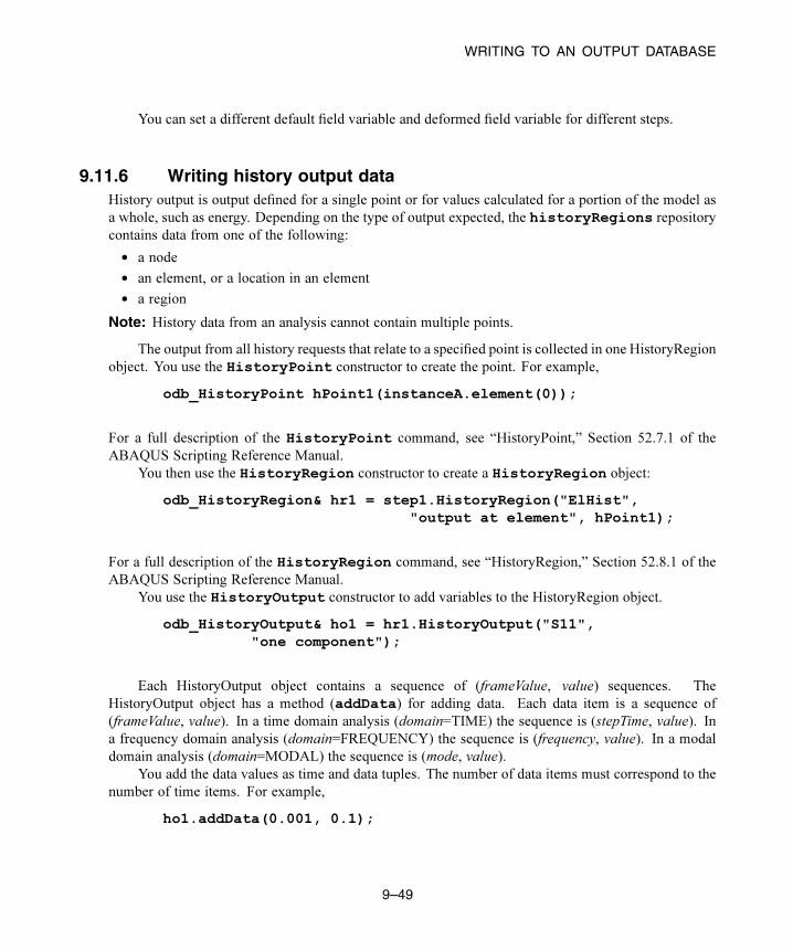
WRITING TO AN OUTPUT DATABASE
You can set a different default field variable and deformed field variable for different steps.
9.11.6 Writing history output data
History output is output defined for a single point or for values calculated for a portion of the model as
a whole, such as energy. Depending on the type of output expected, the historyRegions repository
contains data from one of the following:
• a node
• an element, or a location in an element
• a region
Note: History data from an analysis cannot contain multiple points.
The output from all history requests that relate to a specified point is collected in one HistoryRegion
object. You use the HistoryPoint constructor to create the point. For example,
odb_HistoryPoint hPoint1(instanceA.element(0));
For a full description of the HistoryPoint command, see “HistoryPoint,” Section 52.7.1 of the
ABAQUS Scripting Reference Manual.
You then use the HistoryRegion constructor to create a HistoryRegion object:
odb_HistoryRegion& hr1 = step1.HistoryRegion("ElHist","output at element", hPoint1);
For a full description of the HistoryRegion command, see “HistoryRegion,” Section 52.8.1 of the
ABAQUS Scripting Reference Manual.
You use the HistoryOutput constructor to add variables to the HistoryRegion object.
odb_HistoryOutput& ho1 = hr1.HistoryOutput("S11","one component");
Each HistoryOutput object contains a sequence of (frameValue, value) sequences. The
HistoryOutput object has a method (addData) for adding data. Each data item is a sequence of
(frameValue, value). In a time domain analysis (domain=TIME) the sequence is (stepTime, value). In
a frequency domain analysis (domain=FREQUENCY) the sequence is (frequency, value). In a modal
domain analysis (domain=MODAL) the sequence is (mode, value).
You add the data values as time and data tuples. The number of data items must correspond to the
number of time items. For example,
ho1.addData(0.001, 0.1);
9–49

EXCEPTION HANDLING IN AN OUTPUT DATABASE
// or using two sequences
odb_SequenceFloat timeData;odb_SequenceFloat values;timeData.append(0.001);values.append(0.1);ho1.addData(timeData, values);
// or using a sequence of sequencesodb_SequenceSequenceFloat s11;odb_SequenceFloat value1;value1.append(0.001);value1.append(0.1);s11.append(value1);ho1.addData(s11);
9.12 Exception handling in an output database
Support for C++ exception handling is provided in the API to the output database. For example, in your
C++ program you may wish to customize the error message when an output database was not opened
successfully as follows:
odb_String invalidOdbName = "invalid.odb";try {
odb_Odb& odb = openOdb(invalidOdbName);}catch(odb_BaseException& exc) {
cerr << "odbBaseException caught\n";cerr << "Abaqus error message: " << exc.UserReport()<< endl;cerr << "Customized error message here\n";
}catch(...) {
cerr << "Unknown Exception.\n";}
For more information, see “BaseException object,” Section 55.1 of the ABAQUS Scripting Reference
Manual.
9–50

COMPUTATIONS WITH ABAQUS RESULTS
9.13 Computations with ABAQUS results
The following topics are covered:
• “Rules for the mathematical operations,” Section 9.13.1
• “Valid mathematical operations,” Section 9.13.2
• “Envelope calculations,” Section 9.13.3
9.13.1 Rules for the mathematical operations
Mathematical operations are supported for FieldOutput, FieldValue, and HistoryOutput objects. These
operators allow you to perform linear superposition of ABAQUS results or to create more complex
derived results from ABAQUS results.
The following rules apply:
• The operations are performed on the components of a tensor or vector.
• The invariants are computed from the component values. For example, taking the absolute value
of a tensor can result in negative values of the pressure invariant.
• Operations between FieldOutput, FieldValue, and HistoryOutput objects are not supported.
• Multiplication and division are not supported between two vector objects nor between two tensor
objects.
• The types in an expression must be compatible. For example,
– A vector cannot be added to a tensor.
– A three-dimensional surface tensor cannot be added to a three-dimensional planar tensor.
– INTEGRATION_POINT data cannot be added to ELEMENT_NODAL data.
• If the fields in the expression were obtained using the getSubsetmethod, the same getSubsetoperations must have been applied in the same order to obtain each field.
• Arguments to the trigonometric functions must be in radians.
• Operations on tensors are performed in the local coordinate system, if it is available. Otherwise
the global system is used. ABAQUS assumes that the local coordinate systems are consistent for
operations involving more than one tensor.
• Operations between FieldValue objects associated with different locations in the model are allowed
only if the data types are the same. If the locations in the model differ, the FieldValue computed
will not be associated with a location. If the local coordinate systems of the FieldValue objects are
not the same, the local coordinate systems of both fieldValues will be disregarded and the fieldValue
computed will have no local coordinate system.
9–51

COMPUTATIONS WITH ABAQUS RESULTS
• The operations will not be performed on the conjugate data (the imaginary portion of a complex
result).
The FieldOutput operations are significantly more efficient than the FieldValue operators. You can
save the computed FieldOutput objects with the following procedure:
• Create a new FieldOutput object in the output database.
• Use the addData method to add the new computed field objects to the new FieldOutput object.
For example,
// Get fields from odb.odb_StepRepository& stepCon = odb.steps();odb_SequenceFrame& frameCon1 =
stepCon["Step-1"].frames();odb_FieldOutputRepository& fieldCon1 =
frameCon1.get(1).fieldOutputs();odb_SequenceFrame& frameCon2 = stepCon["Step-2"].frame();odb_FieldOutputRepository& fieldCon2 =
frameCon2.get(1).fieldOutputs();odb_FieldOutput& field1 = fieldCon1["U"];odb_FieldOutput& field2 = fieldCon2["U"];
// Compute new field.
odb_FieldOutput deltaDisp = field2 - field1;
// Save new field.
odb_Step& newStep = odb.Step("user", "user defined results",odb_Enum::TIME,1.0);
odb_Frame newFrame = newStep.Frame(0, 0.0);odb_FieldOutput& newField = newFrame.FieldOutput("U",
"delta displacements",odb_Enum::VECTOR);
newField.addData(deltaDisp);
9.13.2 Valid mathematical operations
Table 9–2 describes the abbreviations that are used in mathematical operations.
9–52

COMPUTATIONS WITH ABAQUS RESULTS
Table 9–2 Abbreviations.
Abbreviation Allowable values
all FieldOutput objects, FieldValue objects, HistoryVariable
objects, or floating point numbers
float floating point numbers
FO FieldOutput objects
FV FieldValue objects
HO HistoryOutput objects
Table 9–3 shows the valid operations on FieldOutput objects.
Table 9–3 Valid operations.
Symbol Operation Return
value
all + float addition all
FO + FO FO
FV + FV FV
HO + HO HO
-all unary negation all
all - float subtraction all
FO - FO FO
FV - FV FV
HO + HO HO
all * float multiplication all
all / float division all
abs(all) absolute value all
acos(all) arccosine all
asin(all) arcsine all
atan(all) arctangent all
cos(all) cosine all
9–53
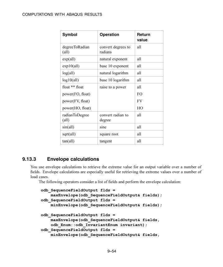
COMPUTATIONS WITH ABAQUS RESULTS
Symbol Operation Return
value
degreeToRadian
(all)
convert degrees to
radians
all
exp(all) natural exponent all
exp10(all) base 10 exponent all
log(all) natural logarithm all
log10(all) base 10 logarithm all
float ** float raise to a power all
power(FO, float) FO
power(FV, float) FV
power(HO, float) HO
radianToDegree
(all)
convert radian to
degree
all
sin(all) sine all
sqrt(all) square root all
tan(all) tangent all
9.13.3 Envelope calculations
You use envelope calculations to retrieve the extreme value for an output variable over a number of
fields. Envelope calculations are especially useful for retrieving the extreme values over a number of
load cases.
The following operators consider a list of fields and perform the envelope calculation:
odb_SequenceFieldOutput flds =maxEnvelope(odb_SequenceFieldOutput& fields);
odb_SequenceFieldOutput flds =minEnvelope(odb_SequenceFieldOutput& fields);
odb_SequenceFieldOutput flds =maxEnvelope(odb_SequenceFieldOutput& fields,odb_Enum::odb_InvariantEnum invariant);
odb_SequenceFieldOutput flds =minEnvelope(odb_SequenceFieldOutput& fields,
9–54

COMPUTATIONS WITH ABAQUS RESULTS
odb_Enum::odb_InvariantEnum invariant);
odb_SequenceFieldOutput flds =maxEnvelope(odb_SequenceFieldOutput& fields,const odb_String& componentLabel);
odb_SequenceFieldOutput flds =minEnvelope(odb_SequenceFieldOutput& fields,const odb_String& componentLabel);
The envelope commands return two FieldOutput objects.
• The first object contains the requested extreme values.
• The second object contains the indices of the fields for which the extreme values were found. The
indices derive from the order in which you supplied the fields to the command.
The optional invariant argument is a odb_Enum::odb_DataTypeEnum specifying the invariant to be used
when comparing vectors or tensors. The optional componentLabel argument is an odb_String specifying
the component of the vector or tensor to be used for selecting the extreme value.
The following rules apply to envelope calculations:
• ABAQUS compares the values using scalar data. If you are looking for the extreme value of a vector
or a tensor, you must supply an invariant or a component label for the selection of the extreme value.
For example, for vectors you can supply the MAGNITUDE invariant and for tensors you can supply
the MISES invariant.
• The fields being compared must be similar. For example,
– VECTOR and TENSOR_3D_FULL fields cannot appear in the same list.
– The output region of all the fields must be the same. All the fields must apply to the whole
model, or all the fields must apply to the same set.
9.13.4 Transformation of results
Transformations of vector and tensor fields are supported for rectangular, cylindrical, and spherical
coordinate systems. The coordinate systems can be fixed or model based. Model-based coordinate
systems refer to nodes for position and orientation. ABAQUS uses the coordinates of the deformed state
to determine a systems origin and orientation for model-based coordinate systems. Transformations
that use a model-based coordinate system can account for large displacements of both the coordinate
system and the structure.
The steps required to transform results are:
• Create the coordinate system.
• Retrieve the field from the database.
• Use the fieldOutput.getTransformedFieldmethod to obtain a new field with the results
in the specified coordinate system.
9–55
IMPROVING THE EFFICIENCY OF YOUR SCRIPTS
• For large displacement of the structure and coordinate system, you must also retrieve the
displacement field at the frame. You must compute this displacement field for the whole model to
ensure that the required displacement information is available.
The following rules apply to the transformation of results:
• Beams, truss, and axisymmetric shell element results will not be transformed.
• The component directions 1, 2, and 3 of the transformed results will correspond to the system
directions X, Y, and Z for rectangular coordinate systems; R, , and Z for cylindrical coordinate
systems; and R, , and for spherical coordinate systems.
Note: Stress results for three-dimensional continuum elements transformed into a cylindrical
system would have the hoop stress in S22, which is consistent with the coordinate system axis
but inconsistent with the stress state for a three-dimensional axisymmetric elements having hoop
stress in S33.
• When you are transforming a tensor, the location or integration point always takes into account the
deformation. The location of the coordinate system depends on the model, as follows:
– If the system is fixed, the coordinate system is fixed.
– If the system is model based, you must supply a displacement field that determines the
instantaneous location and orientation of the coordinate system.
• ABAQUSwill perform transformations of tensor results for shells, membranes, and planar elements
as rotations of results about the element normal at the element result location. The element normal is
the normal computed for the frame associated with the field by ABAQUS, and you cannot redefine
the normal. ABAQUS defines the location of the results location from the nodal locations. You
specify optional arguments if you want to use the deformed nodal locations to transform results.
For rectangular, cylindrical, and spherical coordinate systems the second component direction for
the transformed results will be determined by one of the following:
– The Y-axis in a rectangular coordinate system.
– The -axis in a cylindrical coordinate system.
– The -axis in a spherical coordinate system.
– A user-specified datum axis projected onto the element plane.
If the coordinate system used for projection and the element normal have an angle less than the
specified tolerance (the default is 30°), ABAQUS will use the next axis and generate a warning.
9.14 Improving the efficiency of your scripts
If you are accessing large amounts of data from an output database, you should be aware of potential
inefficiencies in your program and techniques that will help to speed up your scripts.
9–56

IMPROVING THE EFFICIENCY OF YOUR SCRIPTS
• “Creating objects to hold loop counters,” Section 9.14.1
• “Creating objects to hold temporary variables,” Section 9.14.2
• “Using references to objects,” Section 9.14.3
9.14.1 Creating objects to hold loop counters
A program can spend a large proportion of its computation time executing statements inside loops. As a
result, you can make your scripts more efficient if you consider how ABAQUS computes the next value
of a loop counter each time the loop is executed. If possible, you should create an integer or a sequence
object to hold the value of a loop counter. If you use a value derived from an ABAQUS object, the time
taken to calculate the next value can slow your program significantly.
The following example uses the number of nodes in a part instance to determine the range of a loop
counter:
const odb_SequenceNode& nodeSequence = myInstance.nodes();for (int i=0; i < nodeSequence.size() ; i++){
const odb_Node& myNode = nodeSequence[i];nodeLabel = myNode.label();
}
You can make the program more efficient if you create an object to hold the value of the number of nodes.
const odb_SequenceNode& nodeSequence = myInstance.nodes();int numNodes = nodeSequence.size();for (int i=0; i < numNodes; i++){
const odb_Node& myNode = nodeSequence[i];nodeLabel = myNode.label();
}
You can use this technique only if the maximum value of the loop counter remains fixed for the duration
of the loop.
9.14.2 Creating objects to hold temporary variables
To improve the efficiency of scripts that access an output database, you should create objects that will be
used to hold temporary variables that are accessed multiple times while the program is executing. For
example, if the program accesses the temporary variable while inside a loop that is executed many times,
creating an object to hold the variable will speed up your program significantly.
9–57

IMPROVING THE EFFICIENCY OF YOUR SCRIPTS
The following example examines the von Mises stress in each element during a particular frame
of field output. If the stress is greater than a certain maximum value, the program prints the strain
components for the element.
odb_FieldOutputRepository& fieldRep = frame1.fieldOutputs();odb_FieldOutput& stressField = fieldRep.get("S");odb_FieldOutput& strainField = fieldRep.get("LE");const odb_SequenceFieldValue& seqStressVal =
stressField.values();int numFV = seqStressVal.size();int strainComp = 0;for (int loc=0; loc < numFV; loc++) {
const odb_FieldValue stressVal = seqStressVal[loc];if (stressVal.mises() > stressCap) {
cout << "Element label = " << stressVal.elementLabel()<< endl;
cout << "Integration Point = "<< stressVal.integrationPoint() << endl;
const odb_SequenceFieldValue& seqStrainVal =strainField.values();
const odb_FieldValue strainVal = seqStrainVal[loc];const float* const data = strainVal.data(strainComp);cout << " LE : ";for (int comp=0; comp < strainComp; comp++)
cout << data[comp];cout << endl;
}}
In this example every time the script calls the strainField.values method, ABAQUS
must reconstruct the sequence of FieldValue objects. This reconstruction could result in a significant
performance degradation, particularly for a large model.
A slight change in the program greatly improves its performance, as shown in the following
example:
odb_FieldOutputRepository& fieldRep =frame1.fieldOutputs();
odb_FieldOutput& stressField = fieldRep.get("S");odb_FieldOutput& strainField = fieldRep.get("LE");const odb_SequenceFieldValue& seqStressVal =
stressField.values();const odb_SequenceFieldValue& seqStrainVal =
9–58

IMPROVING THE EFFICIENCY OF YOUR SCRIPTS
strainField.values();int numFV = seqStressVal.size();int strainComp = 0;for (int loc=0; loc < numFV; loc++) {
const odb_FieldValue stressVal = seqStressVal[loc];if (stressVal.mises() > stressCap) {
cout << "Element label = " << stressVal.elementLabel()<< endl;
cout << "Integration Point = "<< stressVal.integrationPoint() << endl;
const odb_FieldValue strainVal = seqStrainVal[loc];const float* data = strainVal.data(strainComp);cout << " LE : ";for (int comp = 0; comp < strainComp; comp++)
cout << data[comp];cout << endl;
}}}
Similarly, if you expect to retrieve more than one frame from an output database, you should create
a temporary variable that holds the entire frame repository. You can then provide the logic to retrieve the
desired frames from the repository and avoid recreating the repository each time. For example, executing
the following statements could be very slow:
int numFrames = step1.frames().size();for (int n=0; n < numFrames; n++)
odb_Frame& frame = step1.frames()[n];
Creating a temporary variable to hold the frame repository provides the same functionality and speeds
up the process:
odb_SequenceFrame& frameRepository = step1.frames();int numFrames = frameRepository.size();for (int n=0; n < numFrames; n++)
odb_Frame& frame = frameRepository[n];
Such a potential loss of performance will not be a problem when accessing a load case frame. Accessing
a load case frame does not result in the creation of a frame repository and, thus, does not suffer from a
corresponding loss of performance.
9–59
EXAMPLE PROGRAMS THAT ACCESS DATA FROM AN OUTPUT DATABASE
9.14.3 Using references to objects
Many functions return a reference to an object rather than an object. Returning a reference is much more
efficient because it avoids unnecessary memory operations. To maintain the efficiency of references,
you should use the reference itself. You should not assign the reference to a new object, since assigning
the reference to a new object creates a copy of the object that is denoted by the reference and invokes
potentially expensive copy constructors. For example,
odb_Instance instance = odb.rootAssembly().instances()["PART-1-1"];
const odb_SequenceNode nodeSequence = myInstance.nodes();
In the above case a copy of the nodeSequence object has to be created in memory.
Many of the methods in the ABAQUS Scripting Interface that provide access to an output database
return a reference to an object rather than the object itself. It is muchmore efficient to modify the previous
example to specify the returned type to be a reference:
odb_Instance& instance = odb.rootAssembly().instances()["PART-1-1"];
const odb_SequenceNode& nodeSequence = myInstance.nodes();
In this case no new object is created and no copy constructors are called.
9.15 Example programs that access data from an output database
The following examples illustrate how you use the output database commands to access data from an
output database:
• “Finding the maximum value of von Mises stress,” Section 9.15.1
• “Creating an output database,” Section 9.15.2
• “Reading data from an output database,” Section 9.15.3
• “Combining model and results data from more than one output database into a single output
database,” Section 9.15.4
• “Decreasing the amount of data in an output database by retaining data at specific frames,”
Section 9.15.5
• “Adding results from one output database into another output database,” Section 9.15.6
• “Stress range for multiple load cases,” Section 9.15.7
• “A C++ version of FELBOW,” Section 9.15.8
9–60

EXAMPLE PROGRAMS THAT ACCESS DATA FROM AN OUTPUT DATABASE
9.15.1 Finding the maximum value of von Mises stress
This example illustrates how you can iterate through an output database and search for the maximum
value of von Mises stress. The program opens the output database specified by the first argument on the
command line and iterates through the following:
• Each step.
• Each frame in each step.
• Each value of von Mises stress in each frame.
In addition, you can supply an optional assembly element set argument from the command line, in which
case the program searches only the element set for the maximum value of von Mises stress.
The following illustrates how you can run the example program from the system prompt. The
program will search the element set ALL ELEMENTS in the viewer tutorial output database for the
maximum value of von Mises stress:
abaqus odbMaxMises.py -odb viewer_tutorial.odb-elset “ ALL ELEMENTS”
Note: If a command line argument is a String that contains spaces, some systems will interpret the String
correctly only if it is enclosed in double quotation marks. For example, “ ALL ELEMENTS”.
You can also run the example with only the -help parameter for a summary of the usage.
Use the following commands to retrieve the example program and the viewer tutorial output
database:
abaqus fetch job=odbMaxMises.Cabaqus fetch job=viewer_tutorial
/***************************************************************odbMaxMises.CCode to determine the location and value of the maximumvon-mises stress in an output database.Usage: abaqus odbMaxMises -odb odbName -elset(optional)
elsetNameRequirements:1. -odb : Name of the output database.2. -elset : Name of the assembly level element set.
Search will be done only for element belongingto this set. If this parameter is not provided,search will be performed over the entire model.
3. -help : Print usage****************************************************************/
9–61

EXAMPLE PROGRAMS THAT ACCESS DATA FROM AN OUTPUT DATABASE
#include <omi_iostream.h>#include <odb_API.h>#include <sys/stat.h>/****************utility functions****************/bool fileExists(const odb_String &string);void rightTrim(odb_String &string,const char* char_set);void printExecutionSummary();/***************************************************************/
int ABQmain(int argc, char **argv){
odb_String odbPath;bool ifOdbName = false;odb_String elsetName;bool ifElset = false;odb_Set myElset;odb_String region = "over the entire model";char msg[256];char *abaCmd = argv[0];
for (int arg = 0; arg<argc; arg++){
if (strncmp(argv[arg],"-o**",2) == 0){
arg++;odbPath = argv[arg];rightTrim(odbPath,".odb");if (!fileExists(odbPath))
{cerr << "**ERROR** output database " << odbPath
<< " does not exist\n" << endl;exit(1);
}ifOdbName = true;
}else if (strncmp(argv[arg],"-e**",2)== 0)
9–62

EXAMPLE PROGRAMS THAT ACCESS DATA FROM AN OUTPUT DATABASE
{arg++;elsetName = argv[arg];ifElset = true;
}else if (strncmp(argv[arg],"-h**",2)== 0)
{printExecutionSummary();exit(0);
}}
if (!ifOdbName){
cerr << "**ERROR** output database name is not provided\n";printExecutionSummary();exit(1);
}// Open the output databaseodb_Odb& myOdb = openOdb(odbPath);odb_Assembly& myAssembly = myOdb.rootAssembly();if (ifElset)
{if (myAssembly.elementSets().isMember(elsetName))
{myElset = myAssembly.elementSets()[elsetName];region = " in the element set : " + elsetName;
}else
{cerr<<"An assembly level elset " << elsetName
<< " does not exist in the output database :"<< myOdb.name() << endl;
myOdb.close();exit(0);
}}
// Initialize maximum values.float maxMises = -0.1;int numFV = 0;int maxElem = 0;odb_String maxStep = "__None__";
9–63
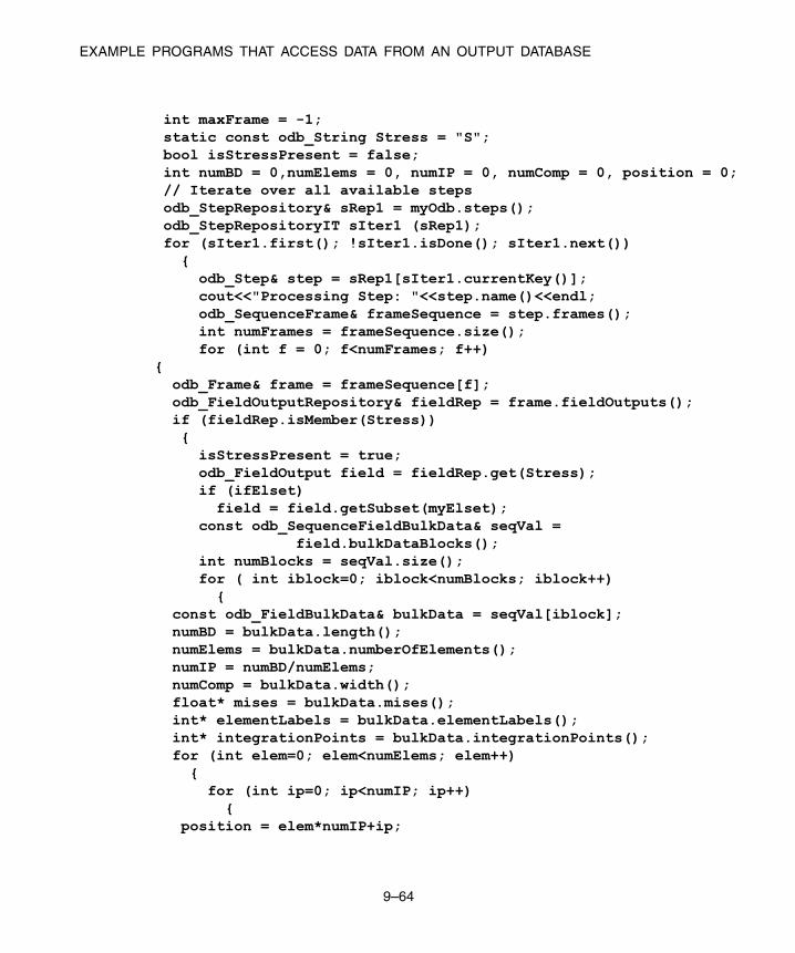
EXAMPLE PROGRAMS THAT ACCESS DATA FROM AN OUTPUT DATABASE
int maxFrame = -1;static const odb_String Stress = "S";bool isStressPresent = false;int numBD = 0,numElems = 0, numIP = 0, numComp = 0, position = 0;// Iterate over all available stepsodb_StepRepository& sRep1 = myOdb.steps();odb_StepRepositoryIT sIter1 (sRep1);for (sIter1.first(); !sIter1.isDone(); sIter1.next())
{odb_Step& step = sRep1[sIter1.currentKey()];cout<<"Processing Step: "<<step.name()<<endl;odb_SequenceFrame& frameSequence = step.frames();int numFrames = frameSequence.size();for (int f = 0; f<numFrames; f++)
{odb_Frame& frame = frameSequence[f];odb_FieldOutputRepository& fieldRep = frame.fieldOutputs();if (fieldRep.isMember(Stress)){
isStressPresent = true;odb_FieldOutput field = fieldRep.get(Stress);if (ifElset)
field = field.getSubset(myElset);const odb_SequenceFieldBulkData& seqVal =
field.bulkDataBlocks();int numBlocks = seqVal.size();for ( int iblock=0; iblock<numBlocks; iblock++)
{const odb_FieldBulkData& bulkData = seqVal[iblock];numBD = bulkData.length();numElems = bulkData.numberOfElements();numIP = numBD/numElems;numComp = bulkData.width();float* mises = bulkData.mises();int* elementLabels = bulkData.elementLabels();int* integrationPoints = bulkData.integrationPoints();for (int elem=0; elem<numElems; elem++)
{for (int ip=0; ip<numIP; ip++)
{position = elem*numIP+ip;
9–64

EXAMPLE PROGRAMS THAT ACCESS DATA FROM AN OUTPUT DATABASE
float misesData = mises[position];if (misesData > maxMises)
{maxMises = misesData;maxElem = elementLabels[elem];maxStep = step.name();maxFrame = frame.frameId();
}}
}}
}}
}if (isStressPresent)
{cout << "Maximum von Mises stress " << region
<< " is " << maxMises << " in element "<< maxElem << endl;
cout << "Location: frame # " << maxFrame << " step: "<< maxStep << endl;
}else
{cout << " Stress output is not available in the "
<< "output database : " << myOdb.name() << endl;}
// close the output database before exiting the programmyOdb.close();return(0);
}
bool fileExists(const odb_String &string){
bool exists = false;struct stat buf;if (stat(string.CStr(),&buf)==0)
exists = true;return exists;
}
9–65

EXAMPLE PROGRAMS THAT ACCESS DATA FROM AN OUTPUT DATABASE
void rightTrim(odb_String &string,const char* char_set){
int length = string.Length();if (string.Find(char_set)==length)
string.append(odb_String(char_set));}
void printExecutionSummary(){
cout << " Code to determine the location and value of the\n"<< " maximum von-mises stress in an output database.\n"<< " Usage: abaqus odbMaxMises -odb odbName \n"<< " -elset(optional), -elsetName\n"<< " Requirements:\n"<< " 1. -odb : Name of the output database.\n"<< " 2. -elset : Name of the assembly level element set.\n"<< " Search will be done only for element \n"<< " belonging to this set.\n"<< " If this parameter is not provided, search \n"<< " will be performed over the entire model.\n"<< " 3. -help : Print usage\n";
}
9.15.2 Creating an output database
The following example illustrates how you can use the ABAQUS C++ API commands to do the
following:
1. Create a new output database.
2. Add model data.
3. Add field data.
4. Add history data.
5. Read history data.
6. Save the output database.
Use the following command to retrieve the example program:
abaqus fetch job=odbWrite
9–66
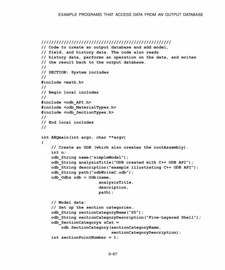
EXAMPLE PROGRAMS THAT ACCESS DATA FROM AN OUTPUT DATABASE
////////////////////////////////////////////////////// Code to create an output database and add model,// field, and history data. The code also reads// history data, performs an operation on the data, and writes// the result back to the output database.//// SECTION: System includes//#include <math.h>//// Begin local includes//#include <odb_API.h>#include <odb_MaterialTypes.h>#include <odb_SectionTypes.h>//// End local includes//
int ABQmain(int argc, char **argv){
// Create an ODB (which also creates the rootAssembly).int n;odb_String name("simpleModel");odb_String analysisTitle("ODB created with C++ ODB API");odb_String description("example illustrating C++ ODB API");odb_String path("odbWriteC.odb");odb_Odb& odb = Odb(name,
analysisTitle,description,path);
// Model data:// Set up the section categories.odb_String sectionCategoryName("S5");odb_String sectionCategoryDescription("Five-Layered Shell");odb_SectionCategory& sCat =
odb.SectionCategory(sectionCategoryName,sectionCategoryDescription);
int sectionPointNumber = 1;
9–67

EXAMPLE PROGRAMS THAT ACCESS DATA FROM AN OUTPUT DATABASE
odb_String sectionPointDescription("Bottom");odb_SectionPoint spBot =
sCat.SectionPoint(sectionPointNumber,sectionPointDescription);
sectionPointNumber = 3;sectionPointDescription = "Middle";odb_SectionPoint spMid =
sCat.SectionPoint(sectionPointNumber,sectionPointDescription);
sectionPointNumber = 5;sectionPointDescription = "Top";odb_SectionPoint spTop =
sCat.SectionPoint(sectionPointNumber,sectionPointDescription);
// Create few materialsodb_MaterialApi materialApi;odb.extendApi(odb_Enum::odb_MATERIAL,materialApi);odb_String materialName("Elastic Material");odb_Material& material_1 =
materialApi.Material(materialName);odb_SequenceSequenceFloat myTable;odb_SequenceFloat myData;myData.append(12000.00);//youngs modulusmyData.append(0.3);//poissons ratiomyTable.append(myData);odb_String type("ISOTROPIC");bool noCompression = false;bool noTension = false;bool temperatureDependency = false;int dependencies = 0;odb_String moduli("LONG_TERM");material_1.Elastic(myTable,
type,noCompression,noTension,temperatureDependency,dependencies,moduli);
//create few sections
9–68

EXAMPLE PROGRAMS THAT ACCESS DATA FROM AN OUTPUT DATABASE
odb_SectionApi sectionApi;odb.extendApi(odb_Enum::odb_SECTION,
sectionApi);odb_String sectionName("Homogeneous Solid Section");float thickness = 2.0;odb_HomogeneousSolidSection& section_1 =
sectionApi.HomogeneousSolidSection(sectionName,materialName,thickness);
// Create a 2-element shell model,//4 integration points, 5 section points.
odb_Part& part1 = odb.Part("part-1",odb_Enum::THREE_D,
odb_Enum::DEFORMABLE_BODY);
odb_SequenceInt nodeLabels;for(n=1; n<7; n++)
nodeLabels.append(n);
double c[6][3] = { {1, 0, 0.0},{2, 0, 0.0},
{2, 1, 0.1},{1, 1, 0.1},
{2, -1, -0.1},{1, -1, -0.1} };
odb_SequenceSequenceFloat nodeCoor;for(n=0; n<nodeLabels.size(); n++) {
odb_SequenceFloat loc;for(int i=0; i<3; i++)
loc.append(c[n][i]);nodeCoor.append(loc);
}odb_String nodeSetName("nset-1");part1.addNodes(nodeLabels,
nodeCoor,nodeSetName);
odb_SequenceInt elLabels;elLabels.append(1);
9–69

EXAMPLE PROGRAMS THAT ACCESS DATA FROM AN OUTPUT DATABASE
elLabels.append(2);odb_SequenceSequenceInt connect;const int numNodePerEl = 4;int conn[2][numNodePerEl] = { {1, 2, 3, 4},
{6, 5, 2, 1} };for(int e=0; e<elLabels.size(); e++) {
odb_SequenceInt l;for(int i=0; i<numNodePerEl; i++)
l.append(conn[e][i]);connect.append(l);
}odb_String elType("S4");odb_String elsetName("eset-1");part1.addElements(elLabels,
connect,elType,elsetName,sCat);
// Instance the part.odb_String partInstanceName("part-1-1");odb_Instance& instance1 =
odb.rootAssembly().Instance(partInstanceName, part1);// create instance level sets for section assignmentelsetName = "Material 1";odb_Set& elset_1 = instance1.ElementSet(elsetName,
elLabels);// section assignment on instanceinstance1.assignSection(elset_1,section_1);// Field data:// Create a step and a frame.odb_String stepName("step-1");odb_String stepDescription("first analysis step");odb_Step& step1 = odb.Step(stepName,
stepDescription,odb_Enum::TIME,
1.0);int frameId = 1;float analysisTime = 0.1;odb_String frameDescription("results frame for time");frameDescription.append(analysisTime);
9–70

EXAMPLE PROGRAMS THAT ACCESS DATA FROM AN OUTPUT DATABASE
odb_Frame frame1 = step1.Frame(frameId,analysisTime,frameDescription);
// Write nodal displacements.odb_String fieldName("U");odb_String fieldDescription("Displacements");odb_FieldOutput& uField =
frame1.FieldOutput(fieldName,fieldDescription,
odb_Enum::VECTOR);
odb_SequenceSequenceFloat dispData;odb_SequenceFloat dispData1[6];// create some displacement valuesfor(n=0; n<6; n++) {
for(int m=1; m<4; m++)dispData1[n].append(n*3+m);
dispData.append(dispData1[n]);}uField.addData(odb_Enum::NODAL,
instance1,nodeLabels,dispData);
// Make this the default deformed field for visualization.
step1.setDefaultDeformedField(uField);
// Write stress tensors (output only available at// top/bottom section points)// The element defined above (S4) has 4 integration points.// Hence, there are 4 stress tensors per element.// Each Field constructor refers to only one layer of// section points.
odb_SequenceSequenceFloat topData;odb_SequenceFloat topData1;for(n=1; n<5; n++)
topData1.append(n);
9–71
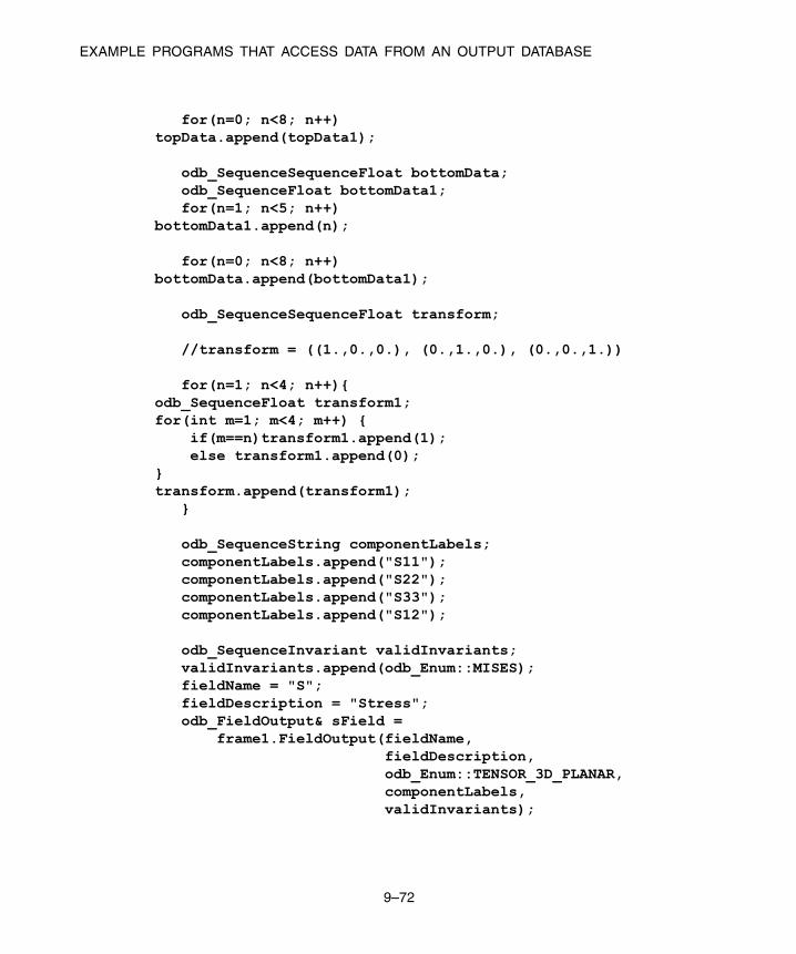
EXAMPLE PROGRAMS THAT ACCESS DATA FROM AN OUTPUT DATABASE
for(n=0; n<8; n++)topData.append(topData1);
odb_SequenceSequenceFloat bottomData;odb_SequenceFloat bottomData1;for(n=1; n<5; n++)
bottomData1.append(n);
for(n=0; n<8; n++)bottomData.append(bottomData1);
odb_SequenceSequenceFloat transform;
//transform = ((1.,0.,0.), (0.,1.,0.), (0.,0.,1.))
for(n=1; n<4; n++){odb_SequenceFloat transform1;for(int m=1; m<4; m++) {
if(m==n)transform1.append(1);else transform1.append(0);
}transform.append(transform1);
}
odb_SequenceString componentLabels;componentLabels.append("S11");componentLabels.append("S22");componentLabels.append("S33");componentLabels.append("S12");
odb_SequenceInvariant validInvariants;validInvariants.append(odb_Enum::MISES);fieldName = "S";fieldDescription = "Stress";odb_FieldOutput& sField =
frame1.FieldOutput(fieldName,fieldDescription,odb_Enum::TENSOR_3D_PLANAR,componentLabels,validInvariants);
9–72
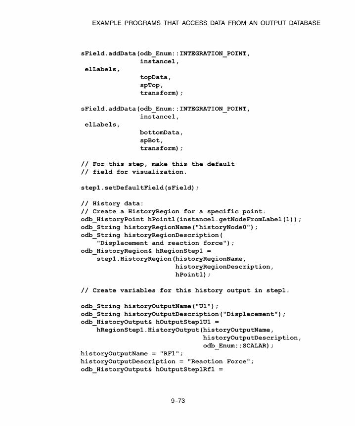
EXAMPLE PROGRAMS THAT ACCESS DATA FROM AN OUTPUT DATABASE
sField.addData(odb_Enum::INTEGRATION_POINT,instance1,
elLabels,topData,spTop,transform);
sField.addData(odb_Enum::INTEGRATION_POINT,instance1,
elLabels,bottomData,spBot,transform);
// For this step, make this the default// field for visualization.
step1.setDefaultField(sField);
// History data:// Create a HistoryRegion for a specific point.odb_HistoryPoint hPoint1(instance1.getNodeFromLabel(1));odb_String historyRegionName("historyNode0");odb_String historyRegionDescription(
"Displacement and reaction force");odb_HistoryRegion& hRegionStep1 =
step1.HistoryRegion(historyRegionName,historyRegionDescription,hPoint1);
// Create variables for this history output in step1.
odb_String historyOutputName("U1");odb_String historyOutputDescription("Displacement");odb_HistoryOutput& hOutputStep1U1 =
hRegionStep1.HistoryOutput(historyOutputName,historyOutputDescription,odb_Enum::SCALAR);
historyOutputName = "RF1";historyOutputDescription = "Reaction Force";odb_HistoryOutput& hOutputStep1Rf1 =
9–73

EXAMPLE PROGRAMS THAT ACCESS DATA FROM AN OUTPUT DATABASE
hRegionStep1.HistoryOutput(historyOutputName,historyOutputDescription,odb_Enum::SCALAR);
// Add history data for step1.
hOutputStep1U1.addData(0.0, 0.0);hOutputStep1Rf1.addData(0.0,0.0);hOutputStep1U1.addData(0.1, 0.1);hOutputStep1Rf1.addData(0.1,0.1);hOutputStep1U1.addData(0.3, 0.3);hOutputStep1Rf1.addData(0.3,0.3);hOutputStep1U1.addData(1.0, 0.5);hOutputStep1Rf1.addData(1.0,0.5);
// Create another step for history data.stepName = "step-2";stepDescription = "second analysis step";odb_Step& step2 = odb.Step(stepName,
stepDescription,odb_Enum::TIME,
1.0);
// Create new history region
odb_HistoryPoint hPoint2(instance1.getNodeFromLabel(1));
odb_HistoryRegion& hRegionStep2 =step2.HistoryRegion(historyRegionName,
historyRegionDescription,hPoint2);
//Create new history outputhistoryOutputName = "U1";historyOutputDescription = "Displacement";odb_HistoryOutput& hOutputStep2U1 =
hRegionStep2.HistoryOutput(historyOutputName,historyOutputDescription,odb_Enum::SCALAR);
historyOutputName = "RF1";
9–74

EXAMPLE PROGRAMS THAT ACCESS DATA FROM AN OUTPUT DATABASE
historyOutputDescription = "Reaction Force";odb_HistoryOutput& hOutputStep2Rf1 =
hRegionStep2.HistoryOutput(historyOutputName,historyOutputDescription,odb_Enum::SCALAR);
// Add history data for the second step.
hOutputStep2U1.addData(1.2, 0.8);hOutputStep2Rf1.addData(1.2,0.9);hOutputStep2U1.addData(1.9, 0.9);hOutputStep2Rf1.addData(1.9,1.1);hOutputStep2U1.addData(3.0, 1.3);hOutputStep2Rf1.addData(3.0,1.3);hOutputStep2U1.addData(4.0, 1.5);hOutputStep2Rf1.addData(4.0,1.5);
// Square the history data U, and store as new history outputhistoryOutputName = "squareU1";historyOutputDescription = "Square of displacements";odb_HistoryOutput& hOutputStep1sumU1 =
hRegionStep1.HistoryOutput(historyOutputName,historyOutputDescription,odb_Enum::SCALAR);
historyOutputName = "squareU2";odb_HistoryOutput& hOutputStep2sumU1 =
hRegionStep2.HistoryOutput(historyOutputName,historyOutputDescription,odb_Enum::SCALAR);
// Get XY Data from the two steps.
odb_HistoryOutputRepository& historyOutputs1 =hRegionStep1.historyOutputs();
historyOutputName = "U1";odb_HistoryOutput& u1FromStep1 =
historyOutputs1[historyOutputName];
odb_HistoryOutputRepository& historyOutputs2 =hRegionStep2.historyOutputs();
9–75

EXAMPLE PROGRAMS THAT ACCESS DATA FROM AN OUTPUT DATABASE
odb_HistoryOutput& u1FromStep2 =historyOutputs2[historyOutputName];
odb_SequenceSequenceFloat hdata1 = u1FromStep1.data();odb_SequenceSequenceFloat hdata2 = u1FromStep2.data();
// Add the squared displacement to the two steps.
for(n=0; n<hdata1.size(); n++){odb_SequenceFloat hdata11=hdata1.get(n);hOutputStep1sumU1.addData(hdata11.get(0),
pow((double)hdata11.get(1),(int)2));}
for(n=0; n<hdata2.size(); n++){odb_SequenceFloat hdata22=hdata2.get(n);hOutputStep2sumU1.addData(hdata22.get(0),
pow((double)hdata22.get(1),(int)2));}
// Save the results in the output database.// Use the Visualization module of ABAQUS/CAE to// view the contents of the output database.
odb.save();odb.close();return 0;
}
9.15.3 Reading data from an output database
This example illustrates how you can print the content of an output database. The example opens the
output database specified on the command line and calls functions that print the following:
• Parts
• Part instances
• The root assembly
9–76

EXAMPLE PROGRAMS THAT ACCESS DATA FROM AN OUTPUT DATABASE
• Connectors
• Connector properties
• Datum coordinate systems
• Nodes
• Elements
• Sets
• Faces
• Sections
• Steps
• Frames
• Fields
• Field values
• Field bulk data
• Field locations
• History regions
• History output
• History points
Use the following command to retrieve the example program:
abaqus fetch job=odbDump
9.15.4 Combining model and results data from more than one output
database into a single output database
This example illustrates how you can read model and results data from several output databases and write
the data into a single output database, which is useful when all the output databases are related to a single
analysis and you want to postprocess them from a single output database. For example, substructure
analyses, as described in “Substructuring,” Section 7.2 of the ABAQUS Analysis User’s Manual.
When you run the program, the following command line parameters are required:
-baseOdb odbName
The name of the output database into which data will be copied.
-copyOdb odbName
The name of the output database from which data will be read.
The following command line parameters are optional:
9–77

EXAMPLE PROGRAMS THAT ACCESS DATA FROM AN OUTPUT DATABASE
-debug
Debug the output generated by this example.
WARNING: If you are extracting data from a large output database, the -debug parameter can
generate large amounts of information.
-step
The name of the step from which to copy. By default, the program copies all field output data from
the last frame in the last step.
-frame
The frame number in the specified step. By default, the program copies all field output data from
the last frame in the last step.
-variable
The name of the field output variable to be copied from the step and frame specified by the -step
and -frame parameters.
If you specify either -step, -frame, or -variable on the command line, you must specify all three
parameters. For example, if you specify a variable to copy, you must also specify a step and a frame
from which it will be copied. You can also run the example with only the -help parameter for a summary
of the usage.
The program has the following limitations:
• The part instances in all the output databases must be compatible. For example, you cannot add a
two-dimensional part instance from an output database to another output database that has three-
dimensional part instances.
• The program copies only deformable part instances, node sets, element sets, and field output. All
the output databases must have the same number of steps and the same number of frames in each
of these steps.
• The ABAQUS C++ API cannot read all the data in an output database. Similarly, the ABAQUS
C++ API cannot write all the data to an output database. For example, theABAQUS C++ API does
not support creation of node-based surface and analytic part instances. As a result, the program
copies only the data supported by the ABAQUS C++ API.
• For large models, using this program to copy field output data for several frames from several output
databases will quickly create a very large output database.
The following example shows how you can use substructureCombine.C with the
substructure example described in “Substructure library utilities,” Section 3.4.8 of the ABAQUS
Verification Manual. Use the following commands to retrieve the example program and the input files
that are required to run the example substructure analysis:
abaqus fetch job=substructureCombine.C
9–78

EXAMPLE PROGRAMS THAT ACCESS DATA FROM AN OUTPUT DATABASE
abaqus fetch job=psuphou1.inpabaqus fetch job=psuphou2.inpabaqus fetch job=psuphou3.inpabaqus fetch job=psuphou4_gen3.inpabaqus fetch job=psuphou4.inp
Run the analyses to generate the first-, second-, and third-level substructures,
abaqus job=psuphou1abaqus job=psuphou2abaqus job=psuphou3abaqus job=psuphou4_gen3
Run the substructure analysis,
abaqus job=psuphou4
You now have the following output databases:
• psuphou4.odb
• psuphou4_1001.odb
• psuphou4_1002.odb
• psuphou4_1001_101.odb
• psuphou4_1002_101.odb
• psuphou4_1001_102.odb
• psuphou4_1002_102.odb
• psuphou4_1001_101_1.odb
• psuphou4_1001_101_2.odb
• psuphou4_1001_101_3.odb
• psuphou4_1002_101_1.odb
• psuphou4_1002_101_2.odb
• psuphou4_1002_101_3.odb
• psuphou4_1001_102_2.odb
• psuphou4_1001_102_1.odb
• psuphou4_1001_102_3.odb
• psuphou4_1002_102_1.odb
• psuphou4_1002_102_2.odb
• psuphou4_1002_102_3.odb
Create the executable,
abaqus make job=substructureCombine.C
9–79
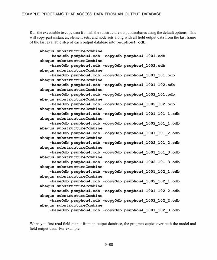
EXAMPLE PROGRAMS THAT ACCESS DATA FROM AN OUTPUT DATABASE
Run the executable to copy data from all the substructure output databases using the default options. This
will copy part instances, element sets, and node sets along with all field output data from the last frame
of the last available step of each output database into psuphou4.odb,
abaqus substructureCombine-baseOdb psuphou4.odb -copyOdb psuphou4_1001.odb
abaqus substructureCombine-baseOdb psuphou4.odb -copyOdb psuphou4_1002.odb
abaqus substructureCombine-baseOdb psuphou4.odb -copyOdb psuphou4_1001_101.odb
abaqus substructureCombine-baseOdb psuphou4.odb -copyOdb psuphou4_1001_102.odb
abaqus substructureCombine-baseOdb psuphou4.odb -copyOdb psuphou4_1002_101.odb
abaqus substructureCombine-baseOdb psuphou4.odb -copyOdb psuphou4_1002_102.odb
abaqus substructureCombine-baseOdb psuphou4.odb -copyOdb psuphou4_1001_101_1.odb
abaqus substructureCombine-baseOdb psuphou4.odb -copyOdb psuphou4_1002_101_1.odb
abaqus substructureCombine-baseOdb psuphou4.odb -copyOdb psuphou4_1001_101_2.odb
abaqus substructureCombine-baseOdb psuphou4.odb -copyOdb psuphou4_1002_101_2.odb
abaqus substructureCombine-baseOdb psuphou4.odb -copyOdb psuphou4_1001_101_3.odb
abaqus substructureCombine-baseOdb psuphou4.odb -copyOdb psuphou4_1002_101_3.odb
abaqus substructureCombine-baseOdb psuphou4.odb -copyOdb psuphou4_1001_102_1.odb
abaqus substructureCombine-baseOdb psuphou4.odb -copyOdb psuphou4_1002_102_1.odb
abaqus substructureCombine-baseOdb psuphou4.odb -copyOdb psuphou4_1001_102_2.odb
abaqus substructureCombine-baseOdb psuphou4.odb -copyOdb psuphou4_1002_102_2.odb
abaqus substructureCombine-baseOdb psuphou4.odb -copyOdb psuphou4_1001_102_3.odb
When you first read field output from an output database, the program copies over both the model and
field output data. For example,
9–80
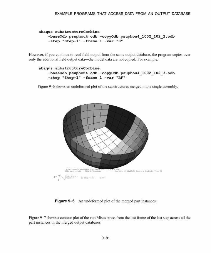
EXAMPLE PROGRAMS THAT ACCESS DATA FROM AN OUTPUT DATABASE
abaqus substructureCombine-baseOdb psuphou4.odb -copyOdb psuphou4_1002_102_3.odb-step "Step-1" -frame 1 -var "S"
However, if you continue to read field output from the same output database, the program copies over
only the additional field output data—the model data are not copied. For example,
abaqus substructureCombine-baseOdb psuphou4.odb -copyOdb psuphou4_1002_102_3.odb-step "Step-1" -frame 1 -var "RF"
Figure 9–6 shows an undeformed plot of the substructures merged into a single assembly.
Step: Step-1Increment 1: Step Time = 1.000
POINT LOADED HEMISPHERICAL SHELL --- 3 X 4 X 4 S4R5ODB: master.odb ABAQUS/Standard 6.4-PR11 Mon Jun 02 16:28:51 Eastern Daylight Time 20
12
3
Figure 9–6 An undeformed plot of the merged part instances.
Figure 9–7 shows a contour plot of the von Mises stress from the last frame of the last step across all the
part instances in the merged output databases.
9–81

EXAMPLE PROGRAMS THAT ACCESS DATA FROM AN OUTPUT DATABASE
(Ave. Crit.: 75%)SNEG, (fraction = -1.0)S, Mises
+1.212e+03+1.518e+03+1.825e+03+2.132e+03+2.439e+03+2.745e+03+3.052e+03+3.359e+03+3.666e+03+3.972e+03+4.279e+03+4.586e+03+4.893e+03
at elem PART-1-1_test_1001_101_3_odb.80003000 node 980000064Min +1.212e+03
at elem PART-1-1_test_1001_102_1_odb.80003000 node 980000064Max +4.893e+03
Step: Step-1Increment 1: Step Time = 1.000Primary Var: S, MisesDeformed Var: U Deformation Scale Factor: +2.182e+01
POINT LOADED HEMISPHERICAL SHELL --- 3 X 4 X 4 S4R5ODB: master.odb ABAQUS/Standard 6.4-PR11 Mon Jun 02 16:28:51 Eastern Daylight Time 20
12
3
Figure 9–7 A contour plot of von Mises stress from the merged output database.
9.15.5 Decreasing the amount of data in an output database by retaining
data at specific frames
This example illustrates how you can decrease the size of an output database. In most cases a large
output database results from excessive field output being generated over a large number of frames.
TheABAQUS C++ API does not support the deletion of data from an output database; however, you
can use this example program to copy data from select frames into a second output database created by a
datacheck analysis that has identical model data. The program uses addData to copy data at specified
frames from the large output database into the new output database. The addData method works only
when the model data in the two output databases are identical. For more information, see “addData,”
Section 52.4.6 of the ABAQUS Scripting Reference Manual.
When you run the program, the following command line parameters are required:
-smallOdb odbName
The name of the output database created with a datacheck analysis of the original problem. For
more information, see “Execution procedure for ABAQUS/Standard and ABAQUS/Explicit,”
Section 3.2.2 of the ABAQUS Analysis User’s Manual.
9–82

EXAMPLE PROGRAMS THAT ACCESS DATA FROM AN OUTPUT DATABASE
-largeOdb odbName
The name of the large output database generated by the original problem. The program copies
selected frames from this output database.
The following parameters are optional:
-history
Copy all history output from all available steps in the large output database. By default, history
output is not copied.
WARNING: Copying large amounts of history data can result in the program creating a very large
output database.
-debug
Print a detailed report of all the operations performed during the running of the program. By default,
no debug information is generated.
WARNING: If you are extracting data from a large output database, the debug option can generate
large amounts of information.
You can also run the example with only the -help parameter for a summary of the usage.
The following is an example of how you can use this program in conjunction with the output
database generated by the problem described in “Free ring under initial velocity: comparison of rate-
independent and rate-dependent plasticity,” Section 1.3.4 of the ABAQUS Benchmarks Manual. Use
the following commands to retrieve the example program and the benchmark input file:
abaqus fetch job=odbFilter.Cabaqus fetch job=ringshell.inp
1. Run an analysis using the benchmark input file:
abaqus job=ringshell
This creates an output database called ringshell.odb that contains 100 frames of data.
2. Run a datacheck analysis to obtain a new output database called ringshell_datacheck.odbthat contains the same model data as ringshell.odb:
abaqus job=ringshell_datacheck -input ringshell datacheck
3. Create the executable program:
abaqus make job=odbFilter.C
The program displays the number of frames available in each step. For each step you must specify
the number of increments between frames, which is the frequency at which the data will be copied to the
new output database. Data for the first and last increment in each step are always copied. For example,
9–83
EXAMPLE PROGRAMS THAT ACCESS DATA FROM AN OUTPUT DATABASE
if a step has 100 frames, and you enter a frame interval of 37, the program will copy data for frames 0,37, 74, and 100.
The following statement will run the executable program and read data from the small output
database containing only model data and the large output database created by the benchmark example:
abaqus odbFilter -smallOdb ringshell_datacheck -largeOdb ringshell
The program prompts you for the increment between frames:
Results from ODB : ringshell.odb will be filtered & writtento ODB: ringshell_datacheckBy default only the first & last increment of a step willbe savedFor each step enter the increment between framesfor example : 3 => frames 0,3,6,..,lastframe will be savedSTEP Step-1 has 101 FramesEnter Increment between frames
Enter 37 to define the increment between frames. The program then reads the data and displays the
frames being processed:
Processing frame # : 0Processing frame # : 37Processing frame # : 74Processing frame # : 100Filtering successfully completed
9.15.6 Adding results from one output database into another output
database
This example illustrates how you can use C++ to extract data from one or more output databases and
write the data sequentially to an existing output database. The following parameters are required:
-writeOdb odbName
The name of the output database created by the first analysis. The program creates a copy of
this output database with the name Restart_odbName. All the data read from the other output
databases will be copied into this output database.
-readOdbs odbName
The names of the output databases created by subsequent restart analyses.
The following parameters are optional:
9–84

EXAMPLE PROGRAMS THAT ACCESS DATA FROM AN OUTPUT DATABASE
-mergeSteps
You can use this option to merge data when the first step of the restart analysis is a continuation of
a previous analysis step. When you use this option, the program appends all the frames from the
first step in the restart analysis to the corresponding step in Restart_odbName.If you do not specify -mergeSteps, the data from the first step of the restart analysis will be
copied to a new step name stepName-Restart-N, where N is the position of the specified output
database in the list of names of output databases from which data will be copied.
-history
Copy all history output from all available steps. By default, history output is not copied.
WARNING: Copying large amounts of history data can result in the program creating a very large
output database.
-debug
Print a detailed report of all the operations performed during the merging of the output databases.
By default, no debug information is generated.
WARNING: If you are extracting data from a large output database, the -debug parameter can
generate large amounts of information.
You can also run the example with only the -help parameter for a summary of the usage.
The program has the following limitations:
• The program uses the addData method to copy fields from one output database into another; for
more information, see “addData,” Section 52.4.6 of the ABAQUS Scripting ReferenceManual. The
addData method requires the model data in the two output databases to be identical. As a result,
the program cannot be used to combine any two output databases. You can use the program with
output databases generated with restart analyses; for more information, see “Restarting an analysis,”
Section 7.1 of the ABAQUS Analysis User’s Manual.
• You can use a restart analysis with additional element and node sets, as described in “Restarting
an analysis,” Section 7.1.1 of the ABAQUS Analysis User’s Manual. The odbJoin program will
copy data from these new sets.
The following is an example of how you can use this program in conjunction with the output
databases generated by the problem described in “Axisymmetric forming of a circular cup,” Section 1.3.7
of the ABAQUS Example Problems Manual. Use the following commands to retrieve the program and
the example input file:
abaqus fetch job=odbJoin.Cabaqus fetch job=axiform.inpabaqus fetch job=axiform_restart.inp
9–85

EXAMPLE PROGRAMS THAT ACCESS DATA FROM AN OUTPUT DATABASE
Run the analyses and the subsequent restart analysis. The program will combine the results across the
two resulting output databases:
abaqus job=axiform.inpabaqus job=axiform_restart -oldjob axiform
Create the executable:
abaqus make job=odbJoin.C
Run the program to combine the output databases using the default parameters:
abaqus odbJoin -writeOdb axiform.odb -readOdbs axiform_restart.odb
The following is displayed in the message area:
Creating copy of original odb axiform.odbAll output from restart ODB's will be appended to Restart_axiform.odbProcessing ODB file axiform_restart.odbProcessing step Step-2Processing step Step-3Processing step Step-4Processing step Step-5Restart odb files successfully joined into Restart_axiform.odb
9.15.7 Stress range for multiple load cases
This example illustrates how you can use the envelope operations to compute the stress range over a
number of load cases. The example program does the following:
• For each load case during a specified step, the program collects the S11 components of the stress
tensor fields into a list of scalar fields.
• Computes the maximum andminimum of the S11 stress component using the envelope calculations.
• Computes the stress range using the maximum and minimum values of the stress component.
• Creates a new frame in the step.
• Writes the computed stress range into a new FieldOutput object in the new frame.
Use the following command to retrieve the example program:
abaqus fetch job=stressRange
The fetch command also retrieves an input file that you can use to generate an output database that can
be read by the example program.
////////////////////////////////////////////////////
9–86

EXAMPLE PROGRAMS THAT ACCESS DATA FROM AN OUTPUT DATABASE
// Code to compute a stress range from// all the load cases in a step.//// The stress range is saved to a frame with the// description "Stress Range"
// System includes
// Begin Local Includes#include <odb_API.h>#include <omi_iostream.h>// End Local Includes
odb_FieldOutput computeStressRange( odb_Step& step );
int ABQmain(int argc, char **argv){
if( argc < 3 ) {cerr << "Usage: abaqus stressRange.x odb_name"
<< "step_name"<< endl;
return 1;}
odb_String odbName(argv[1]);odb_String stepName(argv[2]);cout << "Computing for odb \"" << odbName << "\"";cout << " and step \"" << stepName << "\"." << endl;
// compute stress range and save to odbodb_Odb& odb = openOdb(odbName);odb_Step& step = odb.steps()[stepName];odb_FieldOutput range = computeStressRange(step);
// Save the results in the output database.odb_Frame rangeFrame = step.Frame(0, 0, "Stress Range");rangeFrame.FieldOutput(range, "S11 Range");odb.save();odb.close();
9–87

EXAMPLE PROGRAMS THAT ACCESS DATA FROM AN OUTPUT DATABASE
return 0;}
odb_FieldOutputcomputeStressRange(odb_Step& step){
// collect stress fields for all load casesodb_SequenceFieldOutput sFields;odb_LoadCaseRepositoryIT iter(step.loadCases());for( iter.first(); !iter.isDone(); iter.next() ) {
odb_Frame frame = step.getFrame( iter.currentValue() );odb_FieldOutput& stressField = frame.fieldOutputs()["S"];sFields.append(stressField.getScalarField("S11"));
};
// compute maximum and minimum envelopesodb_SequenceFieldOutput maxFields = maxEnvelope(sFields);odb_SequenceFieldOutput minFields = minEnvelope(sFields);
// compute and return rangereturn (maxFields.get(0) - minFields.get(0));
}
9.15.8 A C++ version of FELBOW
This example illustrates the use of a C++ program to read selected element integration point records from
an output database and to postprocess the elbow element results. The program creates X–Y data that can
be plotted with the X–Y plotting capability in ABAQUS/CAE. The program performs the same function
as the FORTRAN program described in “Creation of a data file to facilitate the postprocessing of elbow
element results: FELBOW,” Section 12.1.6 of the ABAQUS Example Problems Manual.
The program reads integration point data for elbow elements from an output database to visualize
one of the following:
1. Variation of an output variable around the circumference of a given elbow element, or
2. Ovalization of a given elbow element.
The program creates either an ASCII file containing X–Y data or a new output database file that can be
viewed using ABAQUS/CAE.
9–88
EXAMPLE PROGRAMS THAT ACCESS DATA FROM AN OUTPUT DATABASE
To use option 2, you must ensure that the integration point coordinates (COORD) are written to
the output database. For option 1 the X-data are data for the distance around the circumference of the
elbow element, measured along the middle surface, and the Y-data are data for the output variable. For
option 2 the X–Y data are the current coordinates of the middle-surface integration points around the
circumference of the elbow element, projected to a local coordinate system in the plane of the deformed
cross-section. The origin of the local system coincides with the center of the cross-section; the plane of
the deformed cross-section is defined as the plane that contains the center of the cross-section.
You should specify the name of the output database during program execution. The program
prompts for additional information, depending on the option that was chosen; this information includes
the following:
• Your choice for storing results (ASCII file or a new output database)
• File name based on the above choice
• The postprocessing option (1 or 2)
• The part name
• The step name
• The frame number
• The element output variable (option 1 only)
• The component of the variable (option 1 only)
• The section point number (option 1 only)
• The element number or element set name
Before program execution, compile and link the C++ program using the ABAQUS/Make procedure:
abaqus make job=felbow.C
After successful compilation, the program’s object code is linked automatically with the ABAQUS object
codes stored in the shared program library and interface library to build the executable program. Refer
to Chapter 4, “Customizing the ABAQUS environment,” of the ABAQUS Installation and Licensing
Guide to see which compile and link commands are used for a particular computer.
Before executing the program, run an analysis that creates an output database file containing the
appropriate output. This analysis includes, for example, output for the elements and the integration point
coordinates of the elements. Execute the program using the following command:
abaqus felbow <filename.odb>
The program prompts for other information, such as the desired postprocessing option, part name, etc.
The program processes the data and produces a text file or a new output database file that contains the
information required to visualize the elbow element results.
“Elastic-plastic collapse of a thin-walled elbow under in-plane bending and internal pressure,”
Section 1.1.2 of the ABAQUS Example Problems Manual, contains several figures that can be created
with the aid of this program.
9–89