volunteered geographic information and the …pure.iiasa.ac.at/14464/1/see chap 7_campelo 2017...

Volunteered Geographic Information and the Future of Geospatial Data

Cláudio Elízio Calazans CampeloFederal University of Campina Grande, Brazil

Michela BertolottoUniversity College Dublin, Ireland

Padraig CorcoranCardiff University, UK

A volume in the Advances in Geospatial Technologies (AGT) Book Series

Published in the United States of America byIGI GlobalInformation Science Reference (an imprint of IGI Global)701 E. Chocolate AvenueHershey PA, USA 17033Tel: 717-533-8845Fax: 717-533-8661 E-mail: [email protected] site: http://www.igi-global.com

Copyright © 2017 by IGI Global. All rights reserved. No part of this publication may be reproduced, stored or distributed in any form or by any means, electronic or mechanical, including photocopying, without written permission from the publisher.Product or company names used in this set are for identification purposes only. Inclusion of the names of the products or companies does not indicate a claim of ownership by IGI Global of the trademark or registered trademark. Library of Congress Cataloging-in-Publication Data

British Cataloguing in Publication DataA Cataloguing in Publication record for this book is available from the British Library.

All work contributed to this book is new, previously-unpublished material. The views expressed in this book are those of the authors, but not necessarily of the publisher.

For electronic access to this publication, please contact: [email protected].

CIP Data PendingISBN: 978-1-5225-2446-5 eISBN: 978-1-5225-2447-2 This book is published in the IGI Global book series Advances in Geospatial Technologies (AGT) (ISSN: 2327-5715; eISSN: 2327-5723)

113

Copyright © 2017, IGI Global. Copying or distributing in print or electronic forms without written permission of IGI Global is prohibited.

Chapter 7

DOI: 10.4018/978-1-5225-2446-5.ch007

ABSTRACT

OpenStreetMap (OSM) is a bottom up community-driven initiative to create a global map of the world. Yet the application of OSM to land use and land cover (LULC) mapping is still largely unexploited due to problems with inconsistencies in the data and harmonization of LULC nomenclatures with OSM. This chapter outlines an automated methodology for creating LULC maps using the nomenclature of two European LULC products: the Urban Atlas (UA) and CORINE Land Cover (CLC). The method is applied to two regions in London and Paris. The results show that LULC maps with a level of detail similar to UA can be obtained for the urban regions, but that OSM has limitations for conversion into the more detailed non-urban classes of the CLC nomenclature. Future work will concentrate on devel-oping additional rules to improve the accuracy of the transformation and building an online system for processing the data.

INTRODUCTION AND BACKGROUND

OpenStreetMap (OSM) is a well-known collaborative mapping project that involves volunteers from all over the world in the creation of a free, global geospatial database. With more than 2.8M registered contributors at the time of writing (July 2016) (http://wiki.openstreetmap.org/wiki/Stats), OSM is one of the most popular projects exemplifying the concept of Volunteered Geographic Information or VGI (See

Using OpenStreetMap to Create Land Use and Land Cover Maps:

Development of an Application

Cidália Costa FonteUniversity of Coimbra, Portugal & INESC

Coimbra, Portugal

Joaquim António PatriarcaINESC Coimbra, Portugal

Marco MinghiniPolitecnico di Milano, Italy

Vyron AntoniouHellenic Military Geographical Service, Greece

Linda SeeInternational Institute for Applied Systems

Analysis, Austria

Maria Antonia BrovelliPolitecnico di Milano, Italy

114

Using OpenStreetMap to Create Land Use and Land Cover Maps

et al., 2016). The availability of the OSM database under a fully open license, which allows anyone to use the data freely and produce derived products, has attracted the interest of a multitude of end users such as industry, professionals, governments and humanitarian organizations (Haklay, Antoniou, Basiouka, Soden, & Mooney, 2014; Soden & Palen, 2014; Olteanu-Raimond et al., 2015; Mooney & Minghini, in press). The success of the project has also attracted the attention of the academic community (Jokar Arsanjani, Zipf, Mooney, & Helbich, 2015), and OSM is now considered to be a research topic on its own.

There are a number of factors that can account for the popularity and massive exploitation of OSM data. The large number of contributors over time has ensured that OSM data have reached a high degree of quality. Many studies exist that have compared OSM data with authoritative datasets and showed that they are of a comparable quality, at least in urban areas where more contributors are active (see e.g. Girres & Touya, 2010; Haklay, 2010; Ciepłuch, Jacob, Mooney, & Winstanley, 2010; Ludwig, Voss, & Krause-Traudes, 2011; Fan, Zipf, Fu, & Neis, 2014; Zheng & Zheng, 2014; Brovelli, Minghini, Molinari, & Zamboni, 2016). The OSM database is also extremely rich, as it includes a variety of thematic layers (with attribute information) that are not traditionally available in other official or authoritative datasets. Lastly, the OSM database is constantly updated and enriched by contributors, and each new version is immediately available for use. In contrast, there are a number of problems related to OSM including an inconsistent spatial coverage (see e.g. Haklay, 2010; Zielstra & Zipf, 2010; Hecht, Kunze, & Hahmann, 2013; Fram, Chistopoulou, & Ellul, 2015; Ribeiro & Fonte, 2015; Brovelli, Minghini, & Molinari, 2016) and positional and thematic inconsistencies, where the latter is due to the relative freedom provided to the contributors in defining object attributes (Ballatore & Mooney, 2015).

Despite these known issues with OSM, the thematic richness of this dataset means that it has great potential for land use and land cover (LULC) mapping. LULC maps are fundamental inputs to many applications ranging from habitat monitoring to ecosystem accounting, among others. These maps are usually generated through the classification of satellite imagery. However, their creation is time consum-ing and therefore their release, even when at greatly detailed level, is only every few years. For example, CORINE Land Cover (CLC) has been produced for 2000, 2006 and 2012, where the 2012 product is still being validated in some countries. The Urban Atlas (UA) is another example of a detailed LULC map but is only available for cities in the European Union. There are also a number of global land cover products available, e.g. GLC-2000 (Mayaux et al., 2006), MODIS (Friedl et al., 2010) and the recently produced GlobeLand30 (Chen et al., 2015), where the latter product has been compared with other authoritative land cover products in Italy and Germany, and good overall agreement was found (Brov-elli et al., 2015; Jokar Arsanjani et al., 2015). Other studies have shown that when these products are compared with one another, there are large spatial disagreements between them (Fritz et al., 2011). The Geo-Wiki crowdsourcing tool has been developed as one way of involving citizens in collecting data on land cover using Google Earth imagery to improve global land cover maps (See et al., 2015). OSM provides an alternative, relatively unexploited source of LULC information that could also be used to generate, verify and validate LULC maps.

Some initial investigations have already been undertaken to convert OSM into LULC maps (Jokar Arsanjani, Helbich, Bakillah, Hagenauer, & Zipf, 2013; Estima & Painho, 2015; Jokar Arsanjani, Mooney, Zipf, & Schauss, 2015; Jokar Arsanjani & Vaz, 2015; Martinho & Fonte, 2015). For example, OSM has been converted to the UA classes for several cities in Europe in order to undertake a comparison of the two products (Jokar Arsanjani et al., 2013; Jokar Arsanjani, Mooney, et al., 2015; Jokar Arsanjani & Vaz, 2015). The results of this comparison varied between 53.6% and 86.2% in terms of overall agree-ment depending upon the city considered. Similar positive results were obtained by Martinho & Fonte

115


(2015) in validating the UA with OSM data and by Estima & Painho (2015) when comparing OSM with CLC in Portugal.

Despite these encouraging outcomes, one of the first challenges when doing this comparison is the need to convert the OSM features into the corresponding nomenclature of the UA and CLC products. This harmonization process is not straightforward because of the way in which the data are collected in OSM. For example, there are frequently overlapping features, which means that these features should be assigned to different LULC classes at the same location. This can be a result of features that contain or cross other features, e.g. a bridge that crosses a water feature, or due to problems with positional accuracy, which results in partial overlapping of features that are inconsistent, e.g. a building footprint that overlaps with a road feature, or the assignment of different tags to the same region due to the sub-jectivity of the volunteers.

Thus, the creation of LULC maps using OSM data requires a solution for dealing with these types of inconsistencies as well as the harmonization of features found in OSM and the classes of LULC maps such as the UA and CLC. Although many of the aforementioned papers discuss these problems, none of them offer automated solutions for dealing with them. Thus, the overall aim of the chapter is to present an automated methodology for converting OSM features into LULC classes using a hierarchical approach, a set of decision rules and geoprocessing within a GIS environment. This procedure will automatically solve a number of inconsistencies found in OSM data when converting the features into LULC classes. The methodology is applied to parts of the cities of London, United Kingdom, and Paris, France, and the results are compared to available LULC maps with different levels of detail, i.e. the UA and CLC.

The remainder of this chapter is structured as follows. Section 2 provides a more technical description of the OSM database, the data model used and how the data are collected. It also offers an overview of the CLC and UA LULC nomenclatures. Section 3 explains the automated methodology developed for OSM conversion into a LULC map, while Section 4 describes the case study where the procedure was tested. The results are then provided in Section 5 and discussed more generally in Section 6, where the conclusions consider outstanding issues and recommendations for future work.

INPUT DATASETS

OSM Data

The OSM project was initiated in 2004 and has continued towards the goal of creating a free and openly-licensed map of the world (Jokar Arsanjani et al., 2015). OSM contains geospatial vector data, i.e. nodes (points), ways (polylines and polygons) and relations (logical collections of two or more nodes, ways or other relations), as well as the associated attributes or tags. Each tag consists of a key and value. Although the main focus of mapping by much of the OSM community has been on capturing road and building features and points of interest, which can be specified by different key value combinations, e.g. “building=residential”, there are also natural and land use key value combinations that can be used to map other land cover and land use features. Thus it is possible to extract land cover and land use information from OSM.

Much of the research on OSM has been on assessing the quality of this data source in comparison to authoritative or reference data, including the study areas in this paper. For example, Haklay (2010) examined the positional accuracy of road features in London and found that many features were within

116


1-2 m of the authoritative data, with average accuracy for different districts in London varying between 3 and 8 m. In another study, Haklay et al. (2010) found that the positional accuracy of OSM in London was high, exceeding 80% overall and with one in four roads having a positional accuracy of between 95 and 100%. A similar exercise was undertaken by Girres and Touya (2010) to compare OSM to authoritative data for France. They found that positional accuracy varied between 5 and 15 m but peaked between 5 and 10 m, similar to that found in London. OSM data have also been compared to LULC maps in previ-ous studies. For example, Jokar Arsanjani et al. (2015) compared OSM with GlobeLand30 and found an overall accuracy of 74%, with higher accuracies of 97% for agricultural areas in Germany. However, the authors also showed that OSM is more accurate than GlobeLand30 in areas where they disagreed using very high resolution satellite imagery. Thus, based on numerous accuracy assessments of OSM in the literature, the authors feel that OSM is accurate enough for LULC mapping.

The Urban Atlas (UA) and CORINE Land Cover (CLC)

The UA, which is officially known as the GMESUA (Global Monitoring for Environment and Security Urban Atlas), provides LULC data for urban areas in all EU member countries as part of the Copernicus Land Monitoring Service (EEA, 2011). The product was developed so that cities across the EU could be compared using a common LULC nomenclature. The UA is currently available for 305 cities for the reference year 2006, where the criterion for inclusion was a population greater than 100K. The minimum mapping unit (MMU) is 0.0025 km2 in urban areas and 1 ha in rural areas, the minimum width of linear elements is 100m, and the positional accuracy is ±5m (EEA 2011). Satellite imagery with a resolution of 2.5m was used for classification, supported by numerous other datasets including topographic maps, navigation data from commercial providers and very high resolution imagery for verification, among others (EEA, 2011). The data are freely available for downloading from the European Environment Agency’s (EEA) website (http://www.eea.europa.eu/data-and-maps/data/urban-atlas#tab-gis-data). In May 2016, the 2012 product was made available for downloading (http://land.copernicus.eu/local/urban-atlas/urban-atlas-2012), increasing the number of cities to 695 by including all urban areas with a population greater than 50K. Validation efforts for this product are still ongoing. Table 1 provides the nomenclature for the UA, up to level 3. Level 1 is the least detailed, e.g. all urban areas are contained in one class, while in level 3 the artificial surfaces are described using 12 classes. A fourth level is still available, but is not considered in this study.

The CLC product is also part of the Copernicus Land Monitoring Service and provides a consistent, comparable, pan-European land cover product (http://land.copernicus.eu/pan-european/corine-land-cover). The first CLC product was developed for the reference year 1990, with subsequent updates in 2000, 2006 and 2012. There are 44 land cover classes in the most detailed level (Table 1), where the nomenclatures of the UA and CLC are clearly compatible. The main difference is that more detailed urban classes can be found in the UA (even without considering the fourth level) and other land cover classes in CLC are more detailed than in the UA, which reflects differences in their overall purpose. The MMU for CLC is larger than the UA at 0.25 km2 for areal objects but the minimum width of 100 m for linear objects is the same. The positional accuracy is 100m and the overall thematic accuracy is greater than 85%. Time series maps of land change are available at a finer MMU of 0.05 km2. The products are generated in both vector and raster format at resolutions of 100m and 250m, respectively. CLC is freely available for downloading from the EEA website (http://land.copernicus.eu/pan-european/corine-land-cover/clc-2012).

117


Table 1. Nomenclatures of UA and CLC

Urban Altas nomenclature CORINE Land Cover nomenclature

Level 1 Level 2 Level 3 Level 1 Level 2 Level 3

1.Artificial Surfaces

1.1 Urban Fabric 1.1.1 Continuous urban fabric 1.1.2 Discontinuous urban fabric 1.1.3 Isolated Structures

1.Artificial Surfaces

1.1 Urban Fabric 1.1.1 Continuous urban fabric 1.1.2 Discontinuous urban fabric

1.2 Industrial, commercial, public, military, private and transport units

1.2.1 Industrial, commercial, public, military and private units 1.2.2 Road and rail network and associated land 1.2.3 Port areas 1.2.4 Airports


1.2.1 Industrial or commercial units 1.2.2 Road and rail network and associated land 1.2.3 Port areas 1.2.4 Airports

1.3 Mine, dump and construction sites

1.3.1 Mineral extraction and dump sites 1.3.3 Construction sites 1.3.4 Land without current use

1.3 Mine, dump and construction sites

1.3.1 Mineral extraction 1.3.2 Dump sites 1.3.3 Construction sites

1.4 Artificial non-agricultural vegetated areas

1.4.1 Green urban areas 1.4.2 Sports and leisure facilities


1.4.1 Green urban areas 1.4.2 Sports and leisure facilities

2. Agricultural, semi-natural areas, wetlands 2.Agricultural areas

2.1 Arable land 2.1.1 Non-irrigated arable land 2.1.2 Permanently irrigated land 2.1.3 Rice fields

2.2 Permanent crops 2.2.1 Vineyards 2.2.2 Fruit trees and berry plantations 2.2.3 Olive groves

2.3 Pastures 2.3.1 Pastures

2.4 Heterogeneous agricultural areas

2.4.1 Annual crops associated with permanent crops 2.4.2 Complex cultivation patterns 2.4.3 Land principally occupied by agriculture, with significant areas of natural vegetation 2.4.4 Agro-forestry areas

3. Forests 3. Forest and semi natural areas

3.1 Forests 3.1.1 Broad-leaved forest 3.1.2 Coniferous forest 3.1.3 Mixed forest

3.2 Scrub and/or herbaceous vegetation associations

3.2.1 Natural grasslands 3.2.2 Moors and heathland 3.2.3 Sclerophyllous vegetation 3.2.4 Transitional woodland-shrub

3.3 Open spaces with little or no vegetation

3.3.1 Beaches, dunes, sands 3.3.2 Bare rocks 3.3.3 Sparsely vegetated areas 3.3.4 Burnt areas 3.3.5 Glaciers and perpetual snow

------- 4. Wetlands 4.1 Inland wetlands 4.1.1 Inland marshes 4.1.2 Peat bogs

4.2 Maritime wetlands

4.2.1 Salt marshes 4.2.2 Salines 4.2.3 Intertidal flats

5. Water 5. Water 5.1 Inland waters 5.1.1 Water courses 5.1.2 Water bodies

5.2 Marine waters 5.2.1 Coastal lagoons 5.2.2 Estuaries 5.2.3 Sea and ocean

118


PROCEDURES AND TOOLS

Methodology

OSM features are converted into a LULC map via a sequence of steps as follows:

Step 1: Associate the key=value combinations available in OSM with the LULC classes in the LULC product of interest, in this case the UA or CLC

Step 2: Choose any user defined values that are necessary for the processingStep 3: Run the conversion processStep 4: Eliminate inconsistencies such as overlapping regions assigned to different classesStep 5: If a MMU is to be considered, then generalize the map so that all regions with smaller areas are

merged with neighboring features

The first step listed above requires that all OSM features to be converted must be associated with corresponding LULC classes. This process can be done for the features that are listed in the OSM Map Features Wiki page (http://wiki.openstreetmap.org/wiki/Map_Features), which represents the official OSM mapping and tagging guide. However, since contributors are free to use keys and values other than the recommended ones, an analysis must always be done for each study area, as different key=value combinations may be available. Moreover, if LULC maps are to be created for the same region using OSM data obtained from different dates (since the data may be changing continuously), an analysis of the available data also needs to be undertaken, so that all of the available data and the changes over time are captured.

The second step refers to the choice of the parameters that may be necessary for the conversion pro-cess. These may be required for a diversity of processes. For example, the linear features that represent objects such as roads, railways or water regions need to be converted into areas, which is typically done by creating buffer zones. Three types of approach can be considered for this conversion:

1. Create a buffer with a predefined width, which is available in the application, for all the lines with the same key=value association. This value is used whenever no user specified values are provided. An example of this may be the use of the typical width of a railway line.

2. Create a buffer with a width chosen by the user for all the lines with the same key=value associa-tion. These parameters need to be provided by the user in step 2 above, prior to the processing. An example of this may be the use of typical widths for the types of roads in a particular region, such as primary or residential roads.

3. Create buffers with different widths for the segments that form a line, with values obtained using spatial analysis. This requires the separation of lines into segments and the identification of the buffer width for each segment, and is executed already as part of step 3 above. An example of this approach is the computation of the distance of each segment forming a road axis to the building polygons. These distances would be associated with each segment, and buffers would then be cre-ated for each segment if the distance to the building is smaller than a predefined or user defined value. The obtained buffers would then be merged.

119


Additional parameters may also be considered, such as the definition of a minimum segment length for specific key=value associations.

The processing of polygonal features may also require the use of parameters inserted by the user. Three types of approach can also be considered in this case, namely:

1. Simple selection of the polygons with the identified combination of key=value to insert into a LULC class.

2. Selection of the polygons with the identified combination of key=value that satisfies predefined or user defined restrictions (such as the polygon area) to insert into a LULC class. An example of this case is the insertion of regions with the key=value association natural/forest to the class Forest only if the area of the polygon is larger than a predefined or chosen value.

3. Selection of the polygons with an identified combination of key=value that satisfies a set of rules related to their neighborhood or topological relations, such as contain or is contained, to insert into a LULC class. Examples of this type of rule are, for example, polygons corresponding to green areas that are associated with recreation areas if they contain equipment such as sports fields (Loai Ali, Schmid, Falomir, & Freksa, 2015).

Step 3 refers to the conversion process that includes the creation of polygons corresponding to lin-ear features, selection of all polygonal features for each LULC class and their conversion into a set of polygons for each class. Figure 1 illustrates the conversion process for class 1.2 (Industrial, commercial, public, military, private and transport units) for both the UA and CLC.

Figure 1. Typical workflow for converting OSM features into UA class 1.2

120


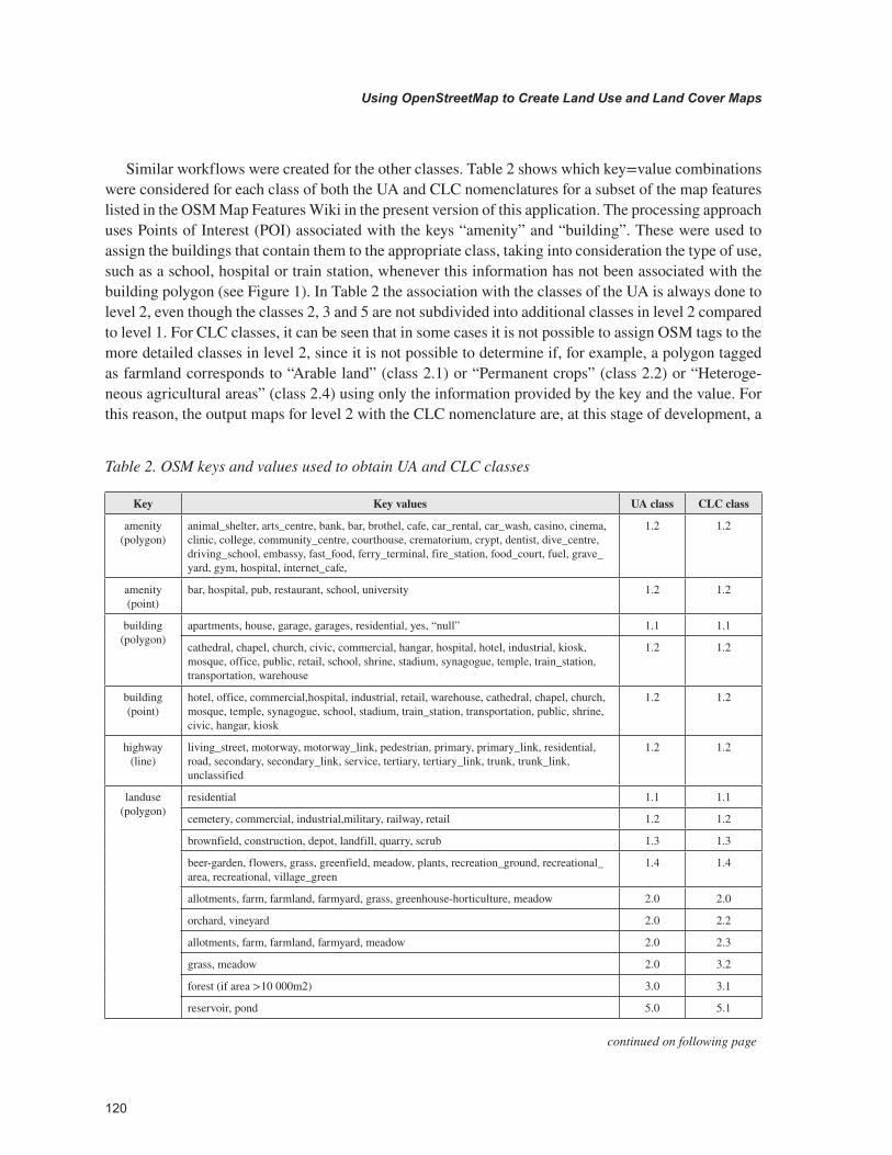
Similar workflows were created for the other classes. Table 2 shows which key=value combinations were considered for each class of both the UA and CLC nomenclatures for a subset of the map features listed in the OSM Map Features Wiki in the present version of this application. The processing approach uses Points of Interest (POI) associated with the keys “amenity” and “building”. These were used to assign the buildings that contain them to the appropriate class, taking into consideration the type of use, such as a school, hospital or train station, whenever this information has not been associated with the building polygon (see Figure 1). In Table 2 the association with the classes of the UA is always done to level 2, even though the classes 2, 3 and 5 are not subdivided into additional classes in level 2 compared to level 1. For CLC classes, it can be seen that in some cases it is not possible to assign OSM tags to the more detailed classes in level 2, since it is not possible to determine if, for example, a polygon tagged as farmland corresponds to “Arable land” (class 2.1) or “Permanent crops” (class 2.2) or “Heteroge-neous agricultural areas” (class 2.4) using only the information provided by the key and the value. For this reason, the output maps for level 2 with the CLC nomenclature are, at this stage of development, a

continued on following page

Table 2. OSM keys and values used to obtain UA and CLC classes

Key Key values UA class CLC class

amenity (polygon)

animal_shelter, arts_centre, bank, bar, brothel, cafe, car_rental, car_wash, casino, cinema, clinic, college, community_centre, courthouse, crematorium, crypt, dentist, dive_centre, driving_school, embassy, fast_food, ferry_terminal, fire_station, food_court, fuel, grave_yard, gym, hospital, internet_cafe,

1.2 1.2

amenity (point)

bar, hospital, pub, restaurant, school, university 1.2 1.2

building (polygon)

apartments, house, garage, garages, residential, yes, “null” 1.1 1.1

cathedral, chapel, church, civic, commercial, hangar, hospital, hotel, industrial, kiosk, mosque, office, public, retail, school, shrine, stadium, synagogue, temple, train_station, transportation, warehouse

1.2 1.2

building (point)

hotel, office, commercial,hospital, industrial, retail, warehouse, cathedral, chapel, church, mosque, temple, synagogue, school, stadium, train_station, transportation, public, shrine, civic, hangar, kiosk

1.2 1.2

highway (line)

living_street, motorway, motorway_link, pedestrian, primary, primary_link, residential, road, secondary, secondary_link, service, tertiary, tertiary_link, trunk, trunk_link, unclassified

1.2 1.2

landuse (polygon)

residential 1.1 1.1

cemetery, commercial, industrial,military, railway, retail 1.2 1.2

brownfield, construction, depot, landfill, quarry, scrub 1.3 1.3

beer-garden, flowers, grass, greenfield, meadow, plants, recreation_ground, recreational_area, recreational, village_green

1.4 1.4

allotments, farm, farmland, farmyard, grass, greenhouse-horticulture, meadow 2.0 2.0

orchard, vineyard 2.0 2.2

allotments, farm, farmland, farmyard, meadow 2.0 2.3

grass, meadow 2.0 3.2

forest (if area >10 000m2) 3.0 3.1

reservoir, pond 5.0 5.1

121


mixture of level 1 and level 2 classes, and whenever it is not possible to differentiate between the level 2 classes, a zero is indicated in the second digit of the used codes for the classes (Table 2). This type of difficulty was found for all classes of CLC except the Artificial Surfaces class (class 1), showing that, without additional spatial analysis and ancillary data, OSM appears to be more appropriate for creating detailed maps of urbanized regions.

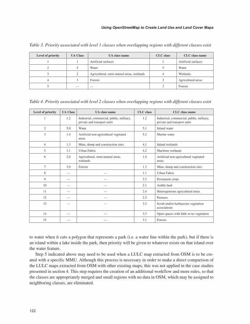
Once the conversion of OSM features into each class is complete, overlapping of different classes may occur. This is due to the nature of OSM and may occur for several reasons, such as erroneous as-signment of regions to the different keys or values by the volunteers, partial overlapping of features due to lack of accuracy in the definition of boundaries or inaccuracies in the conversion of the linear features to polygons. To eliminate this invalid information in the current version of this application, a hierarchi-cal approach is considered in step 4 listed above, which assigns levels of priority to the classes based on their relative importance, size and most common spatial and topological relations. The priorities used here are listed in Tables 3 and 4 for levels 1 and 2 of the UA and CLC nomenclatures, respectively.

Although the use of such a list of priorities solves the problems of inconsistencies, it is not sufficient for solving all types of problems, as the choice of one class over another may change based on the con-text, spatial relations of features and their relative size. For example, it is appropriate to give priority

Table 2. Continued

Key Key values UA class CLC class

leisure (polygon)

adult_gaming_centre, amusement_arcade, dance, hackerspace, ice_rink, sports_centre, stadium, swimming_pool

1.2 1.2

dog_park, garden, park, golf_course, miniature_golf, pitch, playground, summer_camp, track, track, water_park

1.4 1.4

marina 1.4 1.2

Nature_reserve 2.0 3.0

beach_resort 2.0 3.3

swimming_area 5.0 5.0

natural (polygon)

forest (if area <10,000 m2), grassland, park 1.4 1.4

grassland 2.0 2.1

grassland 2.0 2.3

grassland 2.0 2.4

fell, grassland, heath, scrub 2.0 3.2

beach, sand, shingle, bare_rock, scree, glacier 2.0 3.3

mud, wetland 2.0 4.0

forest (if area >10,000 m2), wood 3.0 3.1

bay, water 5.0 5.0

riverbank 5.0 5.1

railway (line) rail 1.2 1.2

waterway (line)

river, riverbank, stream 5.0 5.1

dock 1.2 1.2

122


to water when it cuts a polygon that represents a park (i.e. a water line within the park), but if there is an island within a lake inside the park, then priority will be given to whatever exists on that island over the water feature.

Step 5 indicated above may need to be used when a LULC map extracted from OSM is to be cre-ated with a specific MMU. Although this process is necessary in order to make a direct comparison of the LULC maps extracted from OSM with other existing maps, this was not applied in the case studies presented in section 4. This step requires the creation of an additional workflow and more rules, so that the classes are appropriately merged and small regions with no data in OSM, which may be assigned to neighboring classes, are eliminated.

Table 3. Priority associated with level 1 classes when overlapping regions with different classes exist

Level of priority UA Class UA class name CLC class CLC class name

1 1 Artificial surfaces 1 Artificial surfaces

2 5 Water 5 Water

3 2 Agricultural, semi-natural areas, wetlands 4 Wetlands

4 3 Forests 2 Agricultural areas

5 --- --- 3 Forests

Table 4. Priority associated with level 2 classes when overlapping regions with different classes exist

Level of priority UA Class UA class name CLC class CLC class name

1 1.2 Industrial, commercial, public, military, private and transport units


2 5.0 Water 5.1 Inland water

3 1.4 Artificial non-agricultural vegetated areas

5.2 Marine water

4 1.3 Mine, dump and construction sites 4.1 Inland wetlands

5 1.1 Urban Fabric 4.2 Maritime wetlands

6 2.0 Agricultural, semi-natural areas, wetlands


7 3.0 Forests 1.3 Mine, dump and construction sites

8 --- --- 1.1 Urban Fabric

9 --- --- 2.2 Permanent crops

10 --- --- 2.1 Arable land

11 --- --- 2.4 Heterogeneous agricultural areas

12 --- --- 2.3 Pastures

13 --- --- 3.2 Scrub and/or herbaceous vegetation associations

14 --- --- 3.3 Open spaces with little or no vegetation

15 --- --- 3.1 Forests

123


Application

The procedure for the creation of the LULC maps has been implemented in a fully free and open source environment. Several algorithms for converting OSM data into LULC classes were written in Python, where the flexibility of this programming language allowed different tools for manipulating vector data and the processing of OSM data to be integrated. These tools included GRASS GIS 7, the GDAL/OGR libraries (http://www.gdal.org/) and PostgreSQL 9.5 (https://www.postgresql.org/) with PostGIS 2.2 (http://postgis.net/). The result is a GRASS GIS (https://grass.osgeo.org/) module, available with a Graphical User Interface. In addition, other tools specifically designed to work with OSM data were used such as the osm2pgsql tool (http://wiki.openstreetmap.org/wiki/Osm2pgsql), incorporated in Post-greSQL/PostGIS, and the Osmosis tool (http://wiki.openstreetmap.org/wiki/Osmosis) for the manual preparation of OSM data.

Figure 2 illustrates the transformation process and where each tool was used to obtain the final output. First, Osmosis was used to extract the data for a specific bounding box (London and Paris study areas - see next Section) from a regional OSM file downloaded in July 2016 from Geofabrik (http://www.geofabrik.de/). The preparation of the input data is one of the few tasks that was done manually, but in the future, the user will be able to choose between an XML file (.osm or.pbf) with only the data to be processed or an XML file with data that goes beyond the boundaries of the study area. This is relevant for the next step in which the OSM data are added to PostgreSQL by the osm2pgsql tool. However, if the XML file with OSM data covers a large area, this tool is not capable of executing this in an effective way.

In addition to the file with the OSM data, the script reads a file with the nomenclature to use (UA or CLC) and an SQL file that contains the mapping between each OSM feature and the corresponding LULC classes.

Figure 2. Application workflow for converting OSM features into a LULC map

124


Once all of the inputs are ready, the procedure runs the osm2pgsql tool to add the OSM data into PostgreSQL. The script then reads the database uploaded from the SQL file to the PostgreSQL for each LULC class and obtains all related OSM features, exporting these geometries to GRASS GIS, where the geometric inconsistencies are solved and where some spatial analysis is made, also using tools from the GDAL/OGR Python Bindings. However, in some specific cases (e.g. the calculation of the distance between the roads and the buildings), the spatial operations are made with PostGIS instead of GRASS GIS or GDAL/OGR for reasons of efficiency. After processing all of the features related to each LULC class, these geometries are merged into a single layer and exported as an ESRI Shapefile.

CASE STUDY AREAS FOR DEMONSTRATION OF THE METHODOLOGY

London

Figure 3 shows the area within the city of London (UK), which was chosen as the first area to illustrate the methodology. The 10 km by 10 km bounding box shown in Figure 3 contains a highly urbanized section of London, but with some green space and water features. The spatial coverage of OSM features for the city of London is very good and a direct comparison with the UA will be most meaningful.

Paris

A second study area in Paris (France) was chosen, which is a section from the outskirts of the city; the 10 km by 10 km bounding box of the study area is shown in Figure 4. Like London, Paris also has very good spatial coverage of features in OSM, but in contrast, this portion of Paris has a more rural nature, with other land cover types present. This will allow us to compare the LULC map generated using the methodology outlined previously with both the UA and CLC products.

Results

Figures 5 and 6 show the results for the London study area that correspond to the UA and CLC nomen-clatures, respectively, for levels 1 and 2. Figures 7 and 8 show the results obtained for the second study area, also for UA and CLC nomenclatures, and levels 1 and 2.

To assess the quality of the results obtained with the proposed approach, the obtained maps were overlapped with the original UA and CLC maps, and the areas of the overlapping regions were computed. The comparison of the level 2 classes associated with the overlapping regions of the original maps and the maps extracted from OSM can be seen in Tables 5 and 6 for both study areas, respectively for the UA and the CLC classes.

Tables 5 and 6 show that one of the best mapped classes is water, with match percentages higher than 90% in most cases. It can, however, be seen that for the CLC nomenclature and the London area several regions classified in OSM as water were assigned to other classes in CLC. As can be seen in Figure 6, this occurs mainly because the OSM extracted map was not converted to the CLC MMU and therefore several small water areas are present that are not mapped in CLC. The opposite occurs for

125


the Paris region, where small land regions within the river are mapped in OSM but as they are smaller than the CLC MMU they are not in CLC, resulting in a match in relation to the CLC water area of 74%.

For the London area, which is a highly urbanized region, difficulties were found in separating agri-culture from urban vegetation and dump sites without the application of additional rules. For the Paris region this was less evident, as there are large regions of agricultural areas.

The main findings from the results can be summarized as follows:

1. Overall there is good agreement between the features found in OSM and the UA, even though some classes are more difficult to differentiate, such as different types of vegetation.

Figure 3. Location of the study area in the city of London, United Kingdom, in OSM(data: © OpenStreetMap contributors)

126


2. There are some regions with missing data in OSM although these are only relatively small zones for both study areas. In some cases, data were associated with these regions but they did not provide any LULC information, e.g. administrative boundaries.

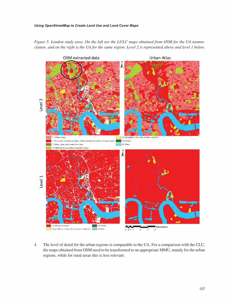
3. The region included in the black circle (see Figures 5 and 6) corresponds to a location where the Olympic Stadium was built for the 2012 Olympic Games that took place in London. The change in this region can be clearly identified in the data extracted from OSM compared to what was found in both the UA, which, according to the metadata associated with the London UA, was created using images from 2006 to 2009, and the 2006 CLC map.

Figure 4. Location of the study area in the city of Paris, France, in OSM(data: © OpenStreetMap contributors)

127


4. The level of detail for the urban regions is comparable to the UA. For a comparison with the CLC, the maps obtained from OSM need to be transformed to an appropriate MMU, mainly for the urban regions, while for rural areas this is less relevant.

Figure 5. London study area: On the left are the LULC maps obtained from OSM for the UA nomen-clature, and on the right is the UA for the same region. Level 2 is represented above and level 1 below.

128


DISCUSSION, CONCLUSION, AND FUTURE DEVELOPMENTS

As already shown in previous research studies (Jokar Arsanjani et al., 2013; Estima & Painho, 2015; Jokar Arsanjani, Mooney, et al., 2015; Jokar Arsanjani & Vaz, 2015; Martinho & Fonte, 2015), OSM can be used to create LULC maps. However, several issues have been encountered during the process

Figure 6. London study area: London study area: On the left are the LULC maps obtained from OSM for the CLC nomenclature, and on the right is CLC for the same region. Level 2 is represented above and level 1 below.

129


of conversion. These need to be documented and solved in order to develop an automated approach for converting OSM data into LULC maps. Here the authors have presented the first version of such an automated process, which uses a mix of predefined, feature-based and analysis-derived parameters.

The process was applied in two selected areas: a densely populated urban area (i.e. London) and a mixed urban/rural landscape (i.e. the outskirts of Paris). In both cases, our process delivered LULC maps that follow the nomenclature of two of the most prominent LULC products that are freely available for

Figure 7. Paris study area: On the left are the LULC maps obtained from OSM for the UA nomenclature, and on the right is UA for the same region. Level 2 is represented above and level 1 below.

130


Europe: the UA and CLC. To achieve this, it was necessary to map the OSM key=values to the existing nomenclatures. Then the outcome was visually and quantitatively compared with the corresponding UA and CLC maps. The results show that, for both study areas, the maps obtained are very similar to the UA. The comparison with CLC shows that without a generalization to the MMU used in CLC, a direct comparison is not appropriate since OSM presents much more detail. From the perspective of the useful-ness and usability of the LULC maps derived from OSM, this higher detail available in OSM represents

Figure 8. Paris study area: On the left are the LULC maps obtained from OSM for the CLC nomenclature, and on the right is CLC for the same region. Level 2 is represented above and level 1 below.

131


a great advantage when LULC maps are to be derived in areas where no accurate LULC products are available, e.g. in underdeveloped or developing countries.

As indicated in the description of the application, the source of the OSM data used in the application was XML files. These files contain the original data created by the volunteers, and have been shown to contain more data than, for example, the shapefiles provided by Geofabrik (Fonte et al., 2016). Moreover, the organization of the data and the tags is different in the shapefiles compared with the.pbf files. For example, values such as “forest”, which should have been associated with the “landuse” key according to the OSM Map Features Wiki, were found to be associated with the “natural” key in the shapefiles. The same thing occurred with “riverbank”, which should have been associated with the key “waterway” but was also associated with the “natural” key in the Geofabrik shapefiles. Thus, to overcome these differ-ences between the original OSM data and the data available in extracts, such as those from Geofabrik, the original XML files were used here instead of the already processed Geofabrik files.

In the case studies presented in this chapter, key=values associations that are not listed in the OSM Map Features Wiki were found, that had to be added to the list of tags, such as “landuse=flowers” or “amenity=conference_center”. These types of problems are due to the fact that, despite guidelines existing

Table 5. Comparison of the area (ha) occupied by level 2 UA classes associated to the overlapping regions in the UA and the map extracted from OSM, for the London (a) and Paris (b) study areas

( a) London Classes assigned to the overlapping regions in the OSM derived map Area in

UA (ha) Match/Row

Sum (%) Match/Area in

UA (%) 11 12 13 14 20 30 50

Classes assigned to the overlapping regions in UA

11 2346 796 16 86 8 2 21 3596 72 65

12 525 2323 214 174 32 8 86 4023 69 58

13 25 51 18 26 5 3 7 161 14 11

14 19 111 5 644 17 5 18 891 79 72

20 5 18 41 23 3 3 9 129 3 2

30 0 0 0 0 0 0 0 0 --- ---

50 12 22 8 5 0 0 1107 1201 96 92

Match/Column Sum (%)

80 70 6 67 4 0 89

(b) Paris Classes assigned to the overlapping regions in the OSM derived map Area in

UA (ha)

Match/Row Sum (%)

Match/Area in UA (%) 11 12 13 14 20 30 50

Classes assigned to the overlapping regions in UA

11 967 106 1 11 50 24 1 1226 83 79

12 186 640 37 20 50 13 3 972 67 66

13 19 24 227 0 45 7 0 330 71 69

14 56 26 0 161 57 6 5 341 52 47

20 108 148 33 43 3545 124 10 4163 88 85

30 21 28 11 44 138 2425 5 2724 91 89

50 3 4 1 1 6 5 221 242 92 91


71 66 73 57 91 93 90

132


on how to tag in the OSM project, a complete freedom in the choice of tags is left to contributors. This presents considerable challenges to the creation of an application that can be widely used by non-experts. Each time the process is run, an analysis of available tags must be undertaken, and the ones that are not assigned to any class need to be identified and assigned to an appropriate class.

The application developed here is already able to produce results, which may be particularly useful for regions where no detailed LULC maps are available. A larger set of OSM tags are exploited than the ones mentioned in Fonte et al. (2016), and some POI have also been added to the procedure. However, additional developments are under preparation, which include:

1. The creation of spatial analysis procedures to enable the choice of the most appropriate class for some key=value associations. Examples of this are the association of a tag such as water to a lake, pond, marina or even the sea, or the association of grass to urban areas, agricultural or natural areas. With context information and information on the size and topological relations with other features, it will be possible to eliminate at least some of the possible choices.

Table 6. Comparison of the area (ha) occupied by level 1 / 2 CLC classes associated to the overlapping regions in CLC and the map extracted from OSM, for the London (a) and Paris (b) study areas

(a) London Classes assigned to the overlapping regions in the OSM derived map Area in

CLC (ha)

Match/Row Sum (%)

Match/Area in CLC (%) 11 12 13 14 20 30 51

Classes assigned to the overlapping regions in CLC

11 2685 1861 64 448 45 8 120 5880 51 46

12 218 1258 228 171 17 13 374 2726 55 46

13 12 77 11 29 2 2 2 156 8 7

14 16 120 0 312 0 0 18 478 67 65

20 0 0 0 0 0 0 0 0 0 0

30 0 0 0 0 0 0 0 0 --- ---

51 2 6 0 1 0 0 740 760 99 97


92 38 4 32 0 0 59

(b) Paris Classes assigned to the overlapping regions in the OSM derived map Area in

CLC (ha)

Match/Row Sum (%)

Match/Area in CLC (%) 11 12 13 14 20 31 32 51

Classes assigned to the overlapping regions in CLC

11 1238 309 20 48 97 7 1 3 1762 72 70

12 31 457 4 16 26 5 0 4 548 84 84

13 0 16 167 0 31 9 0 0 224 75 75

14 5 2 0 131 0 1 0 0 139 94 94

20 52 132 9 37 3480 128 1 9 4109 90 85

31 19 43 310 282 1 0 0 0 2763 0 0

32 5 5 95 0 13 2 23 4 150 16 15

51 9 11 1 7 45 3 0 223 303 75 74


91 47 54 46 90 0 88 91 91

133


2. Development of procedures using spatial analysis to enable the solution of inconsistencies. The hierarchy used to eliminate the existence of more than one class at the same location takes each particular situation and its surroundings into account. A set of rules can be developed to ensure that additional topological relations of features, such as inclusion and contain, context and size of features are also included.

3. Insertion of rules for generalization when a MMU is to be considered. This process will also enable the elimination of some small regions where no data are available in OSM.

The application under development will be made freely available under an open source license, enabling anyone to create a LULC map from OSM data for any part of the world and for different timestamps for the same regions, allowing for analysis of change. Future work will also concentrate on generalizing this approach to any LULC product and building an online processing system, e.g. a Web Processing Service (WPS), to accommodate user requests directly through the Web.

ACKNOWLEDGMENT

The authors would like to acknowledge the support and contribution of COST Actions TD1202 ‘Map-ping and Citizen Sensor’ http://www.citizen-sensor-cost.eu, IC1203 ‘ENERGIC’ http://vgibox.eu/, the ERC CrowdLand project (No. 617754) and FCT project grant UID/MULTI/00308/2013.

REFERENCES

Ballatore, A., & Mooney, P. (2015). Conceptualising the geographic world: The dimensions of negotia-tion in crowdsourced cartography. International Journal of Geographical Information Science, 29(12), 2310–2327. doi:10.1080/13658816.2015.1076825

Brovelli, M. A., Minghini, M., & Molinari, M. (2016). An automated GRASS-based procedure to assess the accuracy of the OpenStreetMap Paris road network. In The International Archives of the Photogram-metry, Remote Sensing and Spatial Information Sciences (Vol. XLI-B7, pp. 919–925). ISPRS Archives. doi:10.5194/isprsarchives-XLI-B7-919-2016

Brovelli, M. A., Minghini, M., Molinari, M., & Zamboni, G. (2016). Positional accuracy assessment of the OpenStreetMap buildings layer through automatic homologous pairs detection: the method and a case study. In The International Archives of the Photogrammetry, Remote Sensing and Spatial Information Sciences (Vol. XLI-B2, pp. 615–620). ISPRS Archives. doi:10.5194/isprsarchives-XLI-B2-615-2016

Brovelli, M. A., Molinari, M. E., Hussein, E., Chen, J., & Li, R. (2015). The First Comprehensive Ac-curacy Assessment of GlobeLand30 at a National Level: Methodology and Results. Remote Sensing, 7(4), 4191-4212. http://doi:10.3390/rs70404191

Chen, J., Chen, J., Liao, A., Cao, X., Chen, L., Chen, X., & Mills, J. et al. (2015). Global land cover mapping at 30 m resolution: A POK-based operational approach. ISPRS Journal of Photogrammetry and Remote Sensing, 103, 7–27. doi:10.1016/j.isprsjprs.2014.09.002

134


Ciepłuch, B., Jacob, R., Mooney, P., & Winstanley, A. (2010). Comparison of the accuracy of OpenStreet-Map for Ireland with Google Maps and Bing Maps. Proceedings of the Ninth International Symposium on Spatial Accuracy Assessment in Natural Resources and Environmental Sciences, 337. Retrieved from http://eprints.nuim.ie/2476/

EEA. (2011). Mapping guide for a European Urban Atlas. Available from: http://www.eea.europa.eu/data-and-maps/data/urban-atlas

Estima, J., & Painho, A. (2015). Investigating the potential of OpenStreetMap for land use/land cover production: A case study for continental Portugal. In J. Jokar Arsanjani, A. Zipf, P. Mooney, & M. Helbich (Eds.), OpenStreetMap in GIScience (pp. 273–293). Cham: Springer International Publishing. doi:10.1007/978-3-319-14280-7_14

Fan, H., Zipf, A., Fu, Q., & Neis, P. (2014). Quality assessment for building footprints data on Open-StreetMap. International Journal of Geographical Information Science, 28(4), 700–719. doi:10.1080/13658816.2013.867495

Fonte, C., Minghini, M., Antoniou, V., See, L., Brovelli, M. A., Patriarca, J., & Milčinski, G. (2016). An automated methodology for converting OSM data into a land use/cover map.Proceedings of the 6th International Conference on Cartography & GIS.

Fram, C., Chistopoulou, K., & Ellul, C. (2015). Assessing the quality of OpenStreetMap building data and searching for a proxy variable to estimate OSM building data completeness.Proceedings of the 23rd GIS Research UK (GISRUK) Conference.

Friedl, M. A., Sulla-Menashe, D., Tan, B., Schneider, A., Ramankutty, N., Sibley, A., & Huang, X. (2010). MODIS Collection 5 global land cover: Algorithm refinements and characterization of new datasets. Remote Sensing of Environment, 114(1), 168–182. doi:10.1016/j.rse.2009.08.016

Fritz, S., See, L., McCallum, I., Schill, C., Obersteiner, M., van der Velde, M., & Achard, F. et al. (2011). Highlighting continued uncertainty in global land cover maps for the user community. Environmental Research Letters, 6(4), 44005. doi:10.1088/1748-9326/6/4/044005

Girres, J.-F., & Touya, G. (2010). Quality assessment of the French OpenStreetMap dataset. Transac-tions in GIS, 14(4), 435–459. doi:10.1111/j.1467-9671.2010.01203.x

Haklay, M. (2010). How good is volunteered geographical information? A comparative study of Open-StreetMap and Ordnance Survey datasets. Environment and Planning. B, Planning & Design, 37(4), 682–703. doi:10.1068/b35097

Haklay, M., Antoniou, V., Basiouka, S., Soden, R., & Mooney, P. (2014). Crowdsourced Geographic Information Use in Government. London: UCL-Geomatics.

Hecht, R., Kunze, C., & Hahmann, S. (2013). Measuring completeness of building footprints in Open-StreetMap over space and time. ISPRS International Journal of Geo-Information, 2(4), 1066–1091. doi:10.3390/ijgi2041066

135


Jokar Arsanjani, J., Helbich, M., Bakillah, M., Hagenauer, J., & Zipf, A. (2013). Toward mapping land-use patterns from volunteered geographic information. International Journal of Geographical Information Science, 27(12), 2264–2278. doi:10.1080/13658816.2013.800871

Jokar Arsanjani, J., Mooney, P., Zipf, A., & Schauss, A. (2015). Quality assessment of the contributed land use information from OpenStreetMap versus authoritative datasets. In J. Jokar Arsanjani, A. Zipf, P. Mooney, & M. Helbich (Eds.), OpenStreetMap in GIScience (pp. 37–58). Cham: Springer International Publishing. doi:10.1007/978-3-319-14280-7_3

Jokar Arsanjani, J., & Vaz, E. (2015). An assessment of a collaborative mapping approach for exploring land use patterns for several European metropolises. International Journal of Applied Earth Observation and Geoinformation, 35(B), 329–337. 10.1016/j.jag.2014.09.009

Jokar Arsanjani, J., Zipf, A., Mooney, P., & Helbich, M. (2015). An introduction to OpenStreetMap in Geographic Information Science: Experiences, research, and applications. In J. Jokar Arsanjani, A. Zipf, P. Mooney, & M. Helbich (Eds.), OpenStreetMap in GIScience (pp. 1–18). Cham: Springer International Publishing. doi:10.1007/978-3-319-14280-7_1

Loai Ali, A., Schmid, F., Falomir, Z., & Freksa, C. (2015). Towards rule-guided classification for Volunteered Geographic Information. In ISPRS Annals of the Photogrammetry, Remote Sensing and Spatial Information Sciences (Vol. II-3/W5). La Grande Motte, France: ISPRS Annals. doi:10.5194/isprsannals-II-3-W5-211-2015

Ludwig, I., Voss, A., & Krause-Traudes, M. (2011). A comparison of the street networks of Navteq and OSM in Germany. In S. Geertman, W. Reinhardt, & F. Toppen (Eds.), Advancing Geoinformation Science for a Changing World (Vol. 1, pp. 65–84). Berlin: Springer Berlin Heidelberg. doi:10.1007/978-3-642-19789-5_4

Martinho, N., & Fonte, C. C. (2015). Assessing the applicability of OpenStreetMap data to validate Land Use/Land Cover Maps (Working Paper No. 5). Coimbra, Portugal: Instituto de Engenharia de Sistemas e Computadores de Coimbra.

Mayaux, P., Eva, H., Gallego, J., Strahler, A. H., Herold, M., & Agrawal, S. … Roy, P. S. (2006). Validation of the global land cover 2000 map. IEEE Transactions on Geoscience and Remote Sens-ing, 44, 1728–1737. Retrieved from http://www.scopus.com/scopus/inward/record.url?eid=2-s2.0-33746330734&partnerID=40

Mooney, P., & Minghini, M. (in press). A review of OpenStreetMap data. In G. Foody, L. See, V. An-toniou, C. C. Fonte, S. Fritz, P. Mooney, & A.-M. Olteanu (Eds.), Mapping and the Citizen Sensor. London, UK: Ubiquity Press.

Olteanu-Raimond, A.-M., Hart, G., Foody, G. M., Touya, G., Kellenberger, T., & Demetriou, D. (2015). The scale of VGI in map production: A perspective of European National Mapping Agencies. Transac-tions in GIS. doi:10.1111/tgis.12189

136


Ribeiro, A., & Fonte, C. C. (2015). Methodology for assessing OpenStreetMap degree of coverage for purposes of land cover mapping. In ISPRS Annals of the Photogrammetry, Remote Sensing and Spatial Information Sciences (Vol. WG II/4). La Grande Motte, France: ISPRS Annals. Retrieved from http://www.isprs-ann-photogramm-remote-sens-spatial-inf-sci.net/II-3-W5/297/2015/isprsannals-II-3-W5-297-2015.pdf

See, L., Fritz, S., Perger, C., Schill, C., McCallum, I., Schepaschenko, D., & Obersteiner, M. et al. (2015). Harnessing the power of volunteers, the internet and Google Earth to collect and validate global spatial information using Geo-Wiki. Technological Forecasting and Social Change, 98, 324–335. doi:10.1016/j.techfore.2015.03.002

See, L., Mooney, P., Foody, G., Bastin, L., Comber, A., Estima, J., & Rutzinger, M. et al. (2016). Crowd-sourcing, citizen science or Volunteered Geographic Information? The current state of crowdsourced geo-graphic information. ISPRS International Journal of Geo-Information, 5(5), 55. doi:10.3390/ijgi5050055

Soden, R., & Palen, L. (2014). From crowdsourced mapping to community mapping: The post-earth-quake work of OpenStreetMap Haiti. In C. Rossitto, L. Ciolfi, D. Martin, & B. Conein (Eds.), COOP 2014 - Proceedings of the 11th International Conference on the Design of Cooperative Systems, 27-30 May 2014, Nice (France) (pp. 311–326). Springer International Publishing. Retrieved from http://link.springer.com/chapter/10.1007/978-3-319-06498-7_19

Zheng, S., & Zheng, J. (2014). Assessing the completeness and positional accuracy of OpenStreetMap in China. In T. Bandrova, M. Konecny, & S. Zlatanova (Eds.), Thematic Cartography for the Society (pp. 171–189). Springer International Publishing. doi:10.1007/978-3-319-08180-9_14

Zielstra, D., & Zipf, A. (2010). A comparative study of proprietary geodata and volunteered geographic information for Germany. Presented at the 13th AGILE International Conference on Geographic Informa-tion Science 2010, Guimarães, Portugal. Retrieved from http://www.agile-online.org/Conference_Paper/CDs/agile_2010/ShortPapers_PDF/142_DOC.pdf

KEY TERMS AND DEFINITIONS

CORINE Land Cover: LULC pan-European land cover product. The first CLC product was devel-oped for the reference year 1990, with subsequent updates in 2000, 2006 and 2012.

Feature Inconsistencies: When features in OSM are converted to LULC maps, there are inconsisten-cies in the data due to overlapping of features, freeform tagging by volunteers that may result in different areas with the same features being tagged in different ways, and due to positional accuracies. These feature inconsistencies need to be handled in order to convert OSM data to a LULC map.

GRASS: A free and open source GIS package.Harmonization of Nomenclatures: The mapping of features in one space (e.g. OSM) to features in

another space (e.g. classes in the Urban Atlas and CORINE Land Cover) in order to allow for conver-sion between nomenclatures.

137


Land Use/Land Cover Map (LULC map): Land use and land cover (LULC) maps provide impor-tant information about urban and rural landscapes and are used in numerous applications from habitat monitoring to ecosystem accounting. Authoritative LULC maps are produced in a semi-automated, top down manner, using satellite imagery, classification algorithms and rigorous validation.

OpenStreetMap (OSM): OSM is a crowdsourced global map of the world created by a community of volunteers. OSM was started by Steve Coast in 2004.

PostGIS: Spatial database extender for PostgreSQL object-relational database.PostgreSQL: Open-source object-relational Database Management Systems.Python: A high level computer programming language.Urban Atlas: LULC data for urban areas in all EU member countries developed for 305 cities for

the reference year 2006, where the criterion for inclusion was a population greater than 100K.Volunteered Geographic Information (VGI): Coined by Goodchild in 2007, VGI is georeferenced

data that are contributed by volunteers, e.g. mapping of features in OSM.

volunteered geographic information and the …pure.iiasa.ac.at/14464/1/see chap 7_campelo 2017...

Documents