Supplementary Information

A comprehensive quantification of global nitrous oxide sources and sinks

Hanqin Tian1, Rongting Xu1, Josep G. Canadell2, Rona L. Thompson3, Wilfried Winiwarter4,5, Parvadha Suntharalingam6, Eric A. Davidson7, Philippe Ciais8, Robert B. Jackson9,10,11, Greet Janssens-Maenhout12,13, Michael J. Prather14, Pierre Regnier15, Naiqing Pan1,16, Shufen Pan1, Glen P. Peters17, Hao Shi1, Francesco N. Tubiello18, Sönke Zaehle19, Feng Zhou20, Almut Arneth21, Gianna Battaglia22, Sarah Berthet23, Laurent Bopp24, Alexander F. Bouwman25,26,27, Erik T. Buitenhuis6,28, Jinfeng Chang8,29, Martyn P. Chipperfield30,31, Shree R. S. Dangal32, Edward Dlugokencky33, James W. Elkins33, Bradley D. Eyre34, Bojie Fu16,35, Bradley Hall33, Akihiko Ito36, Fortunat Joos22, Paul B. Krummel37, Angela Landolfi38,39, Goulven G. Laruelle15, Ronny Lauerwald8,15,40, Wei Li8,41, Sebastian Lienert22, Taylor Maavara42, Michael MacLeod43, Dylan B. Millet44, Stefan Olin45, Prabir K. Patra46,47, Ronald G. Prinn48, Peter A. Raymond42, Daniel J. Ruiz14, Guido R. van der Werf49, Nicolas Vuichard8, Junjie Wang27, Ray F. Weiss50, Kelley C. Wells44, Chris Wilson30,31, Jia Yang51 & Yuanzhi Yao1

1International Center for Climate and Global Change Research, School of Forestry and Wildlife Sciences, Auburn University, Auburn, AL, USA 2Global Carbon Project, CSIRO Oceans and Atmosphere, Canberra, Australian Capital Territory, Australia 3Norsk Institutt for Luftforskning, NILU, Kjeller, Norway 4International Institute for Applied Systems Analysis, Laxenburg, Austria 5 Institute of Environmental Engineering, University of Zielona Góra, Zielona Góra, Poland. 6School of Environmental Sciences, University of East Anglia, Norwich, UK 7Appalachian Laboratory, University of Maryland Center for Environmental Science, Frostburg, MD, USA 8Laboratoire des Sciences du Climat et de l'Environnement, LSCE, CEA CNRS, UVSQ UPSACLAY, Gif sur Yvette, France 9Department of Earth System Science, Stanford University, Stanford, CA, USA 10Woods Institute for the Environment, Stanford University, Stanford, CA, USA 11Precourt Institute for Energy, Stanford University, Stanford, CA, USA 12European Commission, Joint Research Centre (JRC), Ispra, Italy 13Ghent University, Faculty of Engineering and Architecture, Ghent, Belgium 14Department of Earth System Science, University of California Irvine, Irvine, CA, USA 15Department Geoscience, Environment & Society, Université Libre de Bruxelles, Brussels, Belgium 16State Key Laboratory of Urban and Regional Ecology, Research Center for Eco-Environmental Sciences, Chinese Academy of Sciences, Beijing, China 17CICERO Center for International Climate Research, Oslo, Norway 18Statistics Division, Food and Agriculture Organization of the United Nations, Via Terme di Caracalla, Rome, Italy 19Max Planck Institute for Biogeochemistry, Jena, Germany

20Sino-France Institute of Earth Systems Science, Laboratory for Earth Surface Processes, College of Urban and Environmental Sciences, Peking University, Beijing, China

21Karlsruhe Institute of Technology, Institute of Meteorology and Climate Research/Atmospheric Environmental Research, Garmisch-Partenkirchen, Germany 22Climate and Environmental Physics, Physics Institute and Oeschger Centre for Climate Change Research, University of Bern, Bern, Switzerland 23Centre National de Recherches Météorologiques (CNRM), Université de Toulouse, Météo‐France, CNRS, Toulouse, France 24LMD-IPSL, Ecole Normale Supérieure / PSL Université, CNRS; Ecole Polytechnique, Sorbonne Université, Paris, France 25PBL Netherlands Environmental Assessment Agency, The Hague, The Netherlands 26Department of Earth Sciences – Geochemistry, Faculty of Geosciences, Utrecht University, Utrecht, The Netherlands 27Key Laboratory of Marine Chemistry Theory and Technology, Ministry of Education, Ocean University of China, Qingdao, China 28Tyndall Centre for Climate Change Research, School of Environmental Sciences, University of East Anglia, Norwich, UK 29College of Environmental and Resource Sciences, Zhejiang University, Hangzhou, China. 30National Centre for Earth Observation, University of Leeds, Leeds, UK 31Institute for Climate and Atmospheric Science, School of Earth and Environment, University of Leeds, Leeds, UK 32Woods Hole Research Center, Falmouth, MA, USA 33NOAA Global Monitoring Laboratory, Boulder, CO, USA 34Centre for Coastal Biogeochemistry, School of Environment Science and Engineering, Southern Cross University, Lismore, New South Wales, Australia 35Faculty of Geographical Science, Beijing Normal University, Beijing, China 36Center for Global Environmental Research, National Institute for Environmental Studies, Tsukuba, Japan 37Climate Science Centre, CSIRO Oceans and Atmosphere, Aspendale, Victoria, Australia 38 GEOMAR Helmholtz Centre for Ocean Research Kiel, Kiel, Germany 39Istituto di Scienze Marine, Consiglio Nazionale delle Ricerche (CNR), Rome, Italy 40Université Paris-Saclay, INRAE, AgroParisTech, UMR ECOSYS, Thiverval-Grignon, France 41Ministry of Education Key Laboratory for Earth System modeling, Department of Earth System Science, Tsinghua University, Beijing, China 42Yale School of Forestry and Environmental Studies, New Haven, CT, USA 43Land Economy, Environment & Society, Scotland’s Rural College (SRUC), Edinburgh, UK 44Department of Soil, Water, and Climate, University of Minnesota, St Paul, MN, USA 45Department of Physical Geography and Ecosystem Science, Lund University, Lund, Sweden 46Research Institute for Global Change, JAMSTEC, Yokohama, Japan 47Center for Environmental Remote Sensing, Chiba University, Chiba, Japan 48Center for Global Change Science, Massachusetts Institute of Technology, Cambridge, MA, USA 49Faculty of Science, Vrije Universiteit, Amsterdam, Netherlands. 50 Scripps Institution of Oceanography, University of California San Diego, La Jolla, USA

51Department of Forestry, Mississippi State University, Mississippi State, MS, USA

Supporting text

1. Data sources .................................................................................................................................1

2. Detailed description on multiple approaches ...............................................................................3

2.1 NMIP – Global N2O Model Inter-comparison Project ...........................................................3

2.2. The FAOSTAT inventory .....................................................................................................5

2.3. The EDGAR v4.3.2 inventory ...............................................................................................7

2.4. The GAINS inventory ...........................................................................................................8

2.5. The SRNM model .................................................................................................................9

a. Flux upscaling model ............................................................................................................9

b. Global cropland N2O observation dataset ..........................................................................10

c. Gridded input datasets ........................................................................................................11

2.6. Global N flow in aquaculture ..............................................................................................11

2.7. Model-based ocean N2O fluxes ...........................................................................................12

2.8. Net N2O emission from land cover change .........................................................................13

a. Deforestation area and crop/pasture expansion ..................................................................13

c. Secondary tropical forest emissions. ..................................................................................14

2.9. Inland water, estuaries, coastal zones ..................................................................................15

a. Riverine N2O emission simulated by DLEM .....................................................................15

b. The DLEM estimate on N2O emission from global reservoirs ..........................................16

c. Mechanistic Stochastic Modeling of N2O emissions from rivers, lakes, reservoirs and

estuaries ..................................................................................................................................16

d. Coastal zone emissions .......................................................................................................18

2.10. Atmospheric inversion models ..........................................................................................18

3. Atmospheric N2O observations and growth rates for three different atmospheric networks

(NOAA, AGAGE, and CISRO) .........................................................................................21

4. Comparison with the IPCC AR5................................................................................................23

5. Per capita N2O emission at global and regional scales in the recent decade .............................24

Supporting tables

Supplementary Table 1 N2O emissions from global agricultural soils based on multiple bottom-up approaches including the additions of mineral N fertilizer, manure and crop residues, and cultivation of organic soils. .........................................................................................32

Supplementary Table 2 N2O emissions from global total area under permanent meadows and pasture, due to manure N deposition (left on pasture) based on EDGAR v4.3.2, FAOSTAT, and GAINS estimates. ....................................................................................32

Supplementary Table 3 N2O emissions due to global manure management based on multiple bottom-up approaches. .......................................................................................................33

Supplementary Table 4 Aquaculture N2O emissions based on multiple sources. .........................33 Supplementary Table 5 Anthropogenic N2O emissions from the global inland waters based on

process-based models.........................................................................................................34 Supplementary Table 6 Anthropogenic N2O emissions from the global inland waters based on

multiple bottom-up approaches. .........................................................................................34 Supplementary Table 7 Natural N2O emissions from the global inland waters based on process-

based models. .....................................................................................................................35 Supplementary Table 8 Nitrous oxide emissions due to atmospheric N deposition on land based

on multiple bottom-up approaches.....................................................................................35 Supplementary Table 9 Global N2O emissions from waste and waste water based on EDGAR

v4.3.2 and GAINS estimates. .............................................................................................36 Supplementary Table 10 Global N2O emissions from fossil fuel and industry based on multiple

bottom-up approaches. .......................................................................................................36 Supplementary Table 11 Global N2O emissions from biomass burning based on multiple bottom-

up approaches.....................................................................................................................37 Supplementary Table 12 Global oceanic N2O emissions based on multiple models. ...................37 Supplementary Table 13 Global N2O emissions based on multiple top-down approaches. ..........38 Supplementary Table 14 Comparison of terminologies used in this study and previous reports. .39 Supplementary Table 15 Comparison of the global N2O budget in this study with the IPCC AR5.

............................................................................................................................................40 Supplementary Table 16 Simulation experiments in the NMIP (Tian et al.1,17) ............................41 Supplementary Table 17 Information of NMIP models using in this study ..................................41 Supplementary Table 18 Summary of models in ocean N2O inter-comparison ............................42 Supplementary Table 19 Overview of the inversion frameworks that are included in the global

N2O budget.........................................................................................................................42

Supporting figures

Supplementary Fig. 1 Spatial distribution of ten study regions across the globe. .........................43

Supplementary Fig. 2 Per capita N2O emission (kg N capita-1 yr-1) during 2007−2016. ..............44

1

1. Data sources

Bottom-up methods include process-based models (NMIP1 including six process‐based terrestrial

biosphere models, DLEM-only2 for pastureland, five ocean models3-8, one mechanistic stochastic

model9,10), four GHG emission databases [EDGAR v4.3.211, FAOSTAT12, GAINS13, GFED4s14

(only for biomass burning), and one statistical model (SRNM) only for cropland soils15. The top-

down approach includes four independent atmospheric inversion frameworks16. The NMIP result

provides nitrous oxide (N2O) emissions from natural and agricultural soils, defined as soils in

agricultural land, during 1860−2016, with consideration of multiple environmental factors, such

as climate, elevated atmospheric carbon dioxide (CO2), land cover and land use change,

atmospheric nitrogen (N) deposition, mineral N fertilizer, and manure N in cropland17. Mineral N

fertilizer and manure N are mainly applied to cropland, while N deposition can reach soils under

all land uses. Natural soil emissions were estimated by NMIP based on the ensemble mean of six

models (Supplementary Table 16): (1) the Dynamic Land Ecosystem Model (DLEM)18,19, (2)

Land Processes and eXchanges model - Bern (LPX-Bern v1.4)20,21, (3) O-CN22, (4) Organising

Carbon and Hydrology In Dynamic Ecosystems (ORCHIDEE)23, (5) Organising Carbon and

Hydrology In Dynamic Ecosystems-Carbon Nitrogen Phosphorus (ORCHIDEE-CNP)23, and (6)

Vegetation Integrated SImulator for Trace gases (VISIT)24,25 (See more model information in

Tian et al.1,17). Agricultural soil emissions were from manure and fertilizer N applications on

cropland during 1860−20161 and intensively managed grassland (pastures) during 1900−20142.

For ‘Indirect emissions from anthropogenic N additions’, we considered emissions from

atmospheric N deposition and ‘Inland and coastal waters’ N leaching/runoff including five sub-

systems: rivers, lakes, estuaries, reservoirs, and coastal zones. Yao et al.26 estimated N2O

emissions from rivers using the process-based model (DLEM) during 1900−2016 and provided

estimates from reservoirs as well, while emissions determined from the stochastic mechanistic

model of Maavara et al.10 and Lauerwald et al.9 for the river-reservoir-estuary continuum, and

lakes, respectively, were in 2000. Coastal zone emissions were obtained from data compilation

reported in Camillini et al.27 and Murray et al.28. The DLEM model also provided an estimate of

N2O emissions from biomass burning across various biomes (crop residue and savannas,

peatland, tropical forest, temperate forest, and boreal forest) during 1860−2015. A nutrient

budget model for shellfish and finfish29-31 was used to calculate the nutrient flows in aquaculture

2

production systems. For computing the N2O emission we consider the amount of N released to

the environment, i.e. the difference between N intake and N in the harvested fish, which includes

all the nutrient excretion. Estimates of oceanic N2O fluxes are derived from an inter-comparison

of five global ocean biogeochemistry models including Bern-3D3, NEMOv3.6-PISCESv2-gas4,

NEMO-PlankTOM105, UVic2.96, and NEMO-PISCES 3.27.

The EDGAR v4.3.2 applies the IPCC guidelines mostly at Tier-1, but integrates higher tier

information based on available country reporting, mostly from Annex I countries. It provided

data from 1970 to 2012. We updated the data to 2016 based on the global and regional trends

between 2000 and 2012 for each individual category. In EDGAR v4.3.2, ‘Indirect emission from

N deposition’ only represents non-agricultural activities. ‘Waste and waste water’ includes

‘Waste incineration’ and ‘Wastewater handling’. We merged ‘Transportation’, ‘Energy’,

‘Industry’, and ‘Residential and other sectors’ to represent the total emission from ‘Fossil fuel

and industry’. Since the EDGAR v4.3.2 database did not provide the emission of ‘Biomass

burning’ from land use outside of agriculture, here we did not include its estimate of ‘Agriculture

waste burning’ into the data synthesis. The FAOSTAT emissions database of the Food and

Agriculture Organization of the United Nations (FAO) covers emissions of N2O from agriculture

and land use by country and globally, from 1961 to 2017 for agriculture, and from 199012 for

relevant land use categories, i.e, cultivation of histosols, biomass burning, etc., applying only

Tier-1 coefficients32. In addition to the IPCC agriculture burning categories ‘Burning crop

residues’ and ‘Burning savannah’, FAOSTAT also estimates N2O emissions from deforestation

fires, forest fires and peatland fires. Emissions from ‘Fossil fuel and industry’ are directly

adapted from the EDGAR v4.3.2 emission inventory. The GAINS model13 provided N2O

emissions data every five-years (i.e., 1990, 1995, 2000, 2005, 2010, 2015). We assumed the

change between each five-year estimate was linear. To avoid abrupt jumps between 1989 and

1990 during data synthesis, we linearly extrapolated data to 1980 through using estimates in

1990 and 1995 in each sub-sector. ‘Direct soil emissions’ are from synthetic N fertilizer, animal

manure, cultivation of histosols, and crop residues. ‘Indirect emissions from anthropogenic N

additions’ are from ‘N deposition on land’ and ‘Inland and coastal waters’ (i.e., lakes, rivers, and

shelf seas). The source of ‘N deposition on land’ is mainly from agricultural activities, but it

deposited on all global ice-free areas (i.e., agricultural land, forest land, other land uses). The

‘Energy’ emission includes conversion, industry, transport, and domestic. The ‘Industry’

3

emission includes nitric acid plants, adipic acid plants, and caprolactam plants. We merged

‘Energy’ and ‘Industry’ to represent ‘Fossil fuel and industry’ emissions. They also considered

N2O use, but we did not include this sector in the synthesis table. We merged ‘Composting’ and

‘Wastewater’ sectors into ‘Waste and waste water’ to make comparison with the EDGAR v4.3.2

database. In addition, the sector ‘Grazing’ was treated as ‘Manure left on pasture’ to make

comparison. The GFED4s emission inventory14 provided N2O emissions from ‘Biomass burning’

including agricultural waste and other biomass burning (i.e., Savanna, grassland, and shrubland

fires, boreal forest fires, temperate forest fires, deforestation and degradation, and peatland fires)

during 1997−2016.

The spatially-referenced non-linear model SRNM was fitted through considering

environmental factors and N management practices to generate gridded annual EF maps at 5′

spatial resolution, and then to calculate global/regional N2O emissions during 1901−2016

together with time-series N input datasets15. This database provides N2O emissions from global

and regional cropland with the application of synthetic N fertilizer and manure N for the period

1980−2016.

For the top-down constraints on the global and regional N2O emissions for the period

1998−2016, we have used estimates from four independent atmospheric inversion frameworks

(INVICAT, PyVAR, MIROC4-ACTM, and GEOSChem), all of which used the Bayesian

inversion method. Here, two versions of PyVAR were run using different ocean priors (one high

and one low) for determining the sensitivity to the ocean prior. These runs are denoted as

PyVAR-1 and PyVAR-2, respectively. For the top-down global estimate, we used the original

spatial resolution in each framework. For the top-down regional estimate, we interpolated the

coarse resolution into 1° × 1° to cover all land areas in the four frameworks (see details in

section 2.10).

2. Detailed description on multiple approaches

2.1 NMIP – Global N2O Model Inter-comparison Project

Ten process-based Terrestrial Biosphere Models (TBMs) participate in NMIP. In general, N2O

emissions from soil are regulated at two levels, which are the rates of nitrification and

denitrification in the soil and soil physical factors regulating the ratio of N2O to other nitrous

4

gases33. For N input to land ecosystems, all ten models considered the atmospheric N deposition

and biological fixation, nine models with crop N2O module included N fertilizer use, but only six

models considered manure as N input. For vegetation processes, all models included dynamic

algorithms in simulating N allocation to different living tissues and vegetation N turnover, and

simulated plant N uptake using the “Demand and Supply-driven” approach. For soil N processes,

all ten models simulated N leaching according to water runoff rate; however, models are

different in representing nitrification and denitrification processes and the impacts of soil

chemical and physical factors. The differences in simulating nitrification and denitrification

processes are one of the major uncertainties in estimating N2O emissions. Algorithms associated

with N2O emissions in each participating model are briefly described in Appendix A of Tian et

al.17.

All participating models are driven by consistent input datasets (i.e., climate, atmospheric

CO2 concentration, land cover change, atmospheric N deposition, mineral N fertilization, and

manure N application) and implemented seven simulation experiments (SE0 – SE6;

Supplementary Table 17) at the spatial resolution of 0.5° globally covering the period of 1861–

2016 (ref. 1). The SE1 includes all driving factors for models with manure addition, and the SE2

is the experiment including all the driving factors for models except manure N. In the SE0

simulation, driving forces were kept constant at the level in 1860 over the entire simulation

period (1861−2016).

By comparing results from different model scenarios, it is possible to attribute the changed

spatiotemporal variations of soil N2O emissions to the variations of six natural and

anthropogenic factors, namely, climate (CLIM, including precipitation, humidity, temperature

and photosynthetic active radiation changes), atmospheric CO2 concentration (CO2), land cover

change (LCC), atmospheric N deposition (NDEP), mineral N fertilizer use (NFER), and manure

N use in cropland (MANN). In order to understand soil N2O emissions dynamics caused by crop

cultivation, we further separated the global and regional N2O emissions into those derived from

cropland soils and those from soils of other land ecosystems. All soils in other land ecosystems

except cropland were treated as “natural soils” while model simulations were implemented in

this study. Except for cropland, the current NMIP simulations do not include management

5

practices (such as grazing and forest logging) for other managed ecosystems such as pasture,

planted forests and urban.

In this study, we aimed to attribute the impact of single factor on cropland N2O emissions,

thus participating models without providing SE2−SE6 and SE0 results in cropland were

excluded. Here, we included estimates from six process-based models (Supplementary Table 16).

Four models (DLEM, ORCHIDEE, ORCHIDEE-CNP, and VISIT) considered the effects of

manure N application in cropland and ran all the seven simulation experiments (SE0−SE6),

while the other two models (LPX-Bern and O-CN) did not include manure effects and ran six

model experiments (all except SE1). We used four model results (i.e., DLEM, ORCHIDEE,

ORCHIDEE-CNP, and VISIT) to calculate the manure N effect (SE1−SE2). Meanwhile, we

used six model results (i.e., DLEM, LPX-Bern, O-CN, ORCHIDEE, ORCHIDEE-CNP, and

VISIT) to calculate the effects of synthetic N fertilizer use (SE2−SE3) and atmospheric N

deposition (SE3−SE4). The effect of N deposition in natural vegetation was calculated from the

six models mentioned above.

2.2. The FAOSTAT inventory

The FAOSTAT emissions data are computed at Tier 1 following IPCC, 2006, Vol. 4. The overall

equation is as follows:

Direct emissions are estimated at country level, using the formula:

Emission = A * EF (1a)

where emission represents kg N yr-1; A represents amount of N in the following items (annual

synthetic N applications/manure applied to soils/manure left on pasture/manure treated in

manure management systems/crop residue/biomass burned amount) in kg N yr-1; EF = Tier 1,

default IPCC emission factors, expressed in kg N/kg N.

Indirect emissions are estimated at country level, using the formula:

Emission = Av&l * EF (1b)

6

where emission represents kg N yr-1; A v&l represents the fraction of manure/synthetic N

fertilizers that volatize as NH3 and NOx and are lost through runoff and leaching in kg N yr-1; EF

= Tier 1, default IPCC emission factors, expressed in kg N/kg N.

Synthetic N fertilizers: N2O from synthetic fertilizers is produced by microbial processes of

nitrification and denitrification taking place on the addition site (direct emissions), and after

volatilization/redeposition and leaching processes (indirect emissions).

Manure management: The term manure includes both urine and dung (i.e., both liquid and

solid material) produced by livestock. N2O is produced directly by nitrification and

denitrification processes in the manure, and indirectly by N volatilization and redeposition

processes.

Manure applied to soils: N2O is produced by microbial processes of nitrification and

denitrification taking place on the application site (direct emissions), and after

volatilization/redeposition and leaching processes (indirect emissions).

Manure left on pastures: N2O is produced by microbial processes of nitrification and

denitrification taking place on the deposition site (direct emissions), and after

volatilization/redeposition and leaching processes (indirect emissions).

Crop Residue: N2O emissions from crop residues consist of direct and indirect emissions from

N in crop residues left on agricultural fields by farmers and from forages during pasture renewal

(following the definitions in the IPCC guidelines34). Specifically, N2O is produced by microbial

processes of nitrification and denitrification taking place on the deposition site (direct

emissions), and leaching processes (indirect emissions).

Cultivation of organic soils: The FAOSTAT domain “Cultivation of organic soils” contains

estimates of direct N2O emissions associated with the drainage of organic soils – histosols –

under cropland and grazed grassland.

Burning-savanna: N2O emissions from the burning of vegetation biomass in the land cover

types: Savanna, Woody Savanna, Open Shrublands, Closed Shrublands, and Grasslands.

Burning-crop residues: N2O produced by the combustion of a percentage of crop residues burnt

on-site. Burning-biomass: N2O emissions from the burning of vegetation biomass in the land

cover types: Humid tropical forest, other forest, and organic soils.

7

2.3. The EDGAR v4.3.2 inventory

The new online version, EDGAR v4.3.2 incorporates a full differentiation of emission processes

with technology-specific emission factors and additional end-of-pipe abatement measures6 and

as such updates and refines the emission estimates. The emissions are modelled based on latest

scientific knowledge, available global statistics, and methods recommended by IPCC (2006)34.

Official data submitted by the Annex I countries to the United Nations Framework Convention

on Climate Change (UNFCCC) and to the Kyoto Protocol are used to some extent, particularly

regarding control measures implemented since 1990 that are not described by international

statistics.

The N2O emission factor for direct soil emissions of N2O from the use of synthetic fertilizers

and from manure used as fertilizers and from crop residues is taken from IPCC (2006)34, that

updated the default IPCC emission factor in the IPCC Good Practice Guidance (2000) with a

20% lower value. N2O emissions from the use of animal waste as fertilizer are estimated taking

into account both the loss of N that occurs from manure management systems before manure is

applied to soils and the additional N introduced by bedding material. N2O emissions from

fertilizer use and CO2 from urea fertilization are estimated based on IFA and FAO statistics.

N2O emissions from manure management are based on distribution of manure management

systems from Annex I countries reporting to the UNFCCC, Zhou et al.35 for China and IPCC

(2006)34 for the rest of the countries.

Different N2O emission factors are applied to tropical and non-tropical regions. N and dry

matter content of agricultural residues are estimated from the cultivation area and yield for 24

crop types (two types of beans, barley, cassava, cereals, three types of peas, lentils, maize, millet,

oats, two types of potatoes, pulses, roots and tubers, rice, rye, soybeans, sugar beet, sugar cane,

sorghum, wheat and yams) from FAOSTAT (2014) and using emission factors of IPCC (2006)34.

Indirect N2O emissions from leaching and runoff of nitrate are estimated from N input to

agricultural soils as described above. Leaching and runoff are assumed to occur in all agricultural

areas except non-irrigated dryland regions, which are identified with maps of FAO Geonetwork

(2011). The fraction of N lost through leaching and runoff is based on the study of Van Drecht et

al.36. The updated emission factor for indirect N2O emissions from N leaching and run-off from

8

the IPCC (2006) guidelines is selected, while noting that it is 70% lower than the mean value of

the 1996 IPCC Guidelines and the IPCC Good Practice Guidance (IPCC, 1997, 2000).

Indirect N2O emissions from atmospheric deposition of N of NOx and NH3 emissions from

non-agricultural sources, mainly fossil fuel combustion, are estimated using N in NOx and NH3

emissions from these sources as activity data, based on EDGAR v4.3.2 database for these gases.

The same emission factor from IPCC (2006)34 is used for indirect N2O from atmospheric

deposition of N from NH3 and NOx emissions, as for agricultural emissions.

2.4. The GAINS inventory

The methodology adopted for the estimation of current and future greenhouse gas emissions and

the available potential for emission controls follows the standard methodology used by the

Greenhouse Gas - Air Pollution Interactions and Synergies (GAINS) model37. For a given year,

emissions of each pollutant p are calculated as the product of the activity levels, the

“uncontrolled” emission factor in the absence of any emission control measures, the efficiency of

emission control measures and the application rate of such measures:

𝐸𝐸𝑖𝑖,𝑝𝑝 = ∑ 𝐸𝐸𝑖𝑖,𝑗𝑗,𝑎𝑎,𝑡𝑡,𝑝𝑝𝑗𝑗,𝑎𝑎,𝑡𝑡 = ∑ 𝐴𝐴𝑖𝑖,𝑗𝑗,𝑎𝑎𝑒𝑒𝑒𝑒𝑖𝑖,𝑗𝑗,𝑎𝑎,𝑝𝑝𝑗𝑗,𝑎𝑎,𝑡𝑡 (1 − 𝑒𝑒𝑒𝑒𝑒𝑒𝑡𝑡,𝑝𝑝 )𝑋𝑋𝑖𝑖,𝑗𝑗,𝑎𝑎,𝑡𝑡 (2)

where subscripts i,j,a,t,p denote region, sector, activity, abatement technology, and pollutant,

respectively; Ei,p represents emissions of the specific pollutant p in region i; Aj represents

activity in a given sector j; ef represents “uncontrolled” emission factor; eff represents reduction

efficiency; X represents actual implementation rate of the considered abatement.

Results (emissions from all anthropogenic sources) are available in 5-year intervals from 1990

to 2050 (in some regions up to 2070) for each GAINS region, typically comprising one country

to express areas of common legislation also with respect of air pollution. Very large countries

have been further split along administrative areas, while in cases of limited data availability also

groups of countries have been combined into GAINS regions.

For N2O, the fate of emissions abatement is often connected with action taken to control other

pollutants. For example, it may occur that after control (e.g., of NOx emissions), N2O emissions

become higher than in the unabated case. To reflect this effect, negative reduction efficiencies

would need to be used for N2O. As it is difficult to communicate such negative numbers, GAINS

9

has resorted to present “controlled” emission factors instead, which describe the emission factor

of a process after installation of abatement technology.

2.5. The SRNM model

a. Flux upscaling model

The SRNM model38 was applied to simulate direct cropland-N2O emissions. In SRNM, N2O

emissions were simulated from N application rates using a quadratic relationship, with spatially-

variable model parameters that depend on climate, soil properties, and management practices.

The original version of SRNM was calibrated using field observations from China only39. In this

study, we used the global N2O observation dataset to train it to create maps of gridded annual

emission factors of N2O and the associated emissions at 5-minute resolution from 1901 to

201415. The gridded EF and associated direct cropland-N2O emissions are simulated based on the

following equation:

2 , ijt ij ijt ij ijt ijtE N N i= + + ∀α β ε (3a)

where

( ) ( )2 2~ , , ~ ,ij k ijk ijk ij k ijk ijkk k

N x N x ′ ∑ ∑α λ σ β φ σ (3b)

( ) ( ) ( )2 2 2~ , , ~ , , ~ 0,ijk ijk ijk ijk ijk ijk ijtN N Nλ µ ω φ µ ω ε τ′ ′ (3c)

and i denotes the sub-function of N2O emission (i=1, 2, …, I) that applies for a sub-domain

division iΩ of six climate or soil factors, j represents the type of crop (j=1-2, 1 for upland crops

and 2 for paddy rice), k is the index of climate or soil factors (k=1-6, i.e., soil pH, clay content,

soil organic carbon, bulk density, the sum of cumulative precipitation and irrigation, mean daily

air temperature). iΩ denotes a set of the range of multiple xk. Eijt denotes direct N2O emission

flux (kg N ha−1 yr−1) estimated for crop type j in year t in the ith sub-domain, Nijt is N application

rate (kg N ha−1 yr−1), and αij and βij are defined as summation of the product of xk and λijk over k.

The random terms λ and φ are assumed to be independent and normally distributed, representing

10

the sensitivity of α and β to xk. ε is the model error. µ and µ′ are the mean effect of xk for α and

β, respectively. σ, σ′, ω, ω′, andτ are standard deviations. Optimal sub-domain division,

associated parameters mean values and standard deviations were determined by using the

Bayesian Recursive Regression Tree version 2 (BRRT v2)39-41, constrained by the extended

global cropland-N2O observation dataset. The detailed methodological approach of the BRRT v2

is described in Zhou et al.41

b. Global cropland N2O observation dataset

We aggregated cropland N2O flux observation data from 180 globally distributed observation

sites from online databases, on-going observation networks, and peer-reviewed publications.

Chamber-based observations were only included in this dataset. These data repositories are as

follows: the NitroEurope, CarbonEurope, GHG-Europe (EU-FP7), GRACEnet, TRAGnet,

NANORP, and 14 meta-analysis datasets42-55. Four types of data were excluded from our

analysis: (i) observations without a zero-N control for background N2O emission, (ii)

observations from sites that used controlled-release fertilizers or nitrification inhibitors, (iii)

observations not covering the entire crop growing season, (iv) observations made in laboratory or

greenhouse. We then calculated cropland-N2O emissions as the difference between observed

N2O emission (E) and background N2O emission (E0). Values of EF were estimated for each

nonzero N application rate (Na) as direct cropland-N2O emission divided by Na: EF = (E −

E0)/Na. This yielded a global dataset of direct cropland-N2O emissions, N-rate-dependent N2O

EFs and fertilization records from each site (i.e., 1,052 estimates for upland crops from 152 sites

and 154 estimates for paddy rice from 28 sites), along with site-level information on climate,

soils, crop type, and relevant experimental parameters. Total numbers of sites and total

measurements in the dataset were more than doubled those for previous datasets of N2O EF. The

extended global N2O observation network covered most of fertilized croplands, representing a

wide range of environmental conditions globally. For each site in our dataset, the variables

included four broad categories: N2O emissions data, climate data (cumulative precipitation and

mean daily air temperature), soil attributes (soil pH, clay content, SOC, BD), and management-

related or experimental parameters (N application rate, crop type). More details on global

cropland N2O observation dataset can be found in Wang et al.15

11

c. Gridded input datasets

The updated SRNM model was driven by many input datasets, including climate, soil properties,

N inputs (e.g., synthetic N fertilizer, livestock manure and crop residues applied to cropland), as

well as the historical distribution of cropland. Cumulative precipitation and mean daily air

temperature over the growing season were acquired from the CRU TS v3.23 climate dataset43

(0.5-degree resolution), where growing season in each grid cell was identified following Sacks et

al.52 The patterns of SOC, clay content, BD, and soil pH were acquired from the HWSD v1.2

(ref.56, 1-km resolution). Both climate and soil properties were re-gridded at a resolution of 5′ ×

5′ using a first-order conservative interpolation widely used in the CMIP5 model

intercomparison57. Annual cropland area at 5′ spatial resolution from 1901 to 2014 was obtained

from the History Database of the Global Environment (HYDE 3.2.1)58. N inputs of synthetic

fertilizers were generated based on sub-national statistics (i.e., county-, municipal, provincial or

state-levels) of N-fertilizer consumption of 15,593 administrative units from 38 national

statistical agencies and national statistics of the other 197 countries from FAOSTAT. N inputs of

livestock manure and crop residues applied to cropland were provided by Zhang et al.59 and

FAOSTAT, respectively. To compute crop-specific N application rates, we allocated N inputs

for upland crops and paddy rice based on the breakdown (or proportion) of total fertilizer use by

crop from Rosas60. Crop-specific N application rates (Nijt) were finally resampled into grid maps

at 5′ spatial resolution following the dynamic cropland distributions of the HYDE 3.2.1. The

assumption of a maximum combined synthetic + manure + crop residues N application rate was

1,000 kg N ha−1, larger than the previous threshold61 that was only applied for the sum of

synthetic fertilizers and manure.

2.6. Global N flow in aquaculture

We apply a nutrient budget model for shellfish and finfish62-64 to calculate the nutrient flows in

aquaculture production systems. These flows comprise feed inputs, retention in the fish, and

nutrient excretion. Individual species within crustaceans, seaweed, fish and molluscs are

aggregated to the International Standard Statistical Classification of Aquatic Animals and Plants

(ISSCAAP) groups65, for which production characteristics are specified. Feed and nutrient

conversion rates are used for each ISSCAAP group to calculate the feed and nutrient intake from

12

production data from FAO65. Feed types include home-made aquafeeds and commercial

compound feeds with different feed conversion ratios that also vary in time due to efficiency

improvement; in addition, the model accounts for algae in ponds, that are often fertilized with

commercial fertilizers or animal manure, consumed by omnivore fish species like carp. A special

case is the filter-feeding bivalves that filter seston from the water column, and excrete

pseudofeces, feces and dissolved nutrients. Based on production data and tissue/shell nutrient

contents the model computes the nutrient retention in the fish. Using apparent digestibility

coefficients, the model calculates outflows in the form of feces (i.e. particulate nutrients) and

dissolved nutrients. Finally, nutrient deposition in pond systems and recycling is calculated. For

computing the N2O emission we consider the amount of N released to the environment, i.e. the

difference between N intake and N in the harvested fish, which includes all the nutrient

excretion. Since in pond cultures part of that N is managed, we made the amount of N recycling

explicit, as well as ammonia emissions from ponds. This is to avoid double counting when

computing N2O emissions from crop production.

2.7. Model-based ocean N2O fluxes

Oceanic N2O is produced by microbial activity during organic matter cycling in the subsurface

ocean; its production mechanisms display significant sensitivity to ambient oxygen level. In the

oxic ocean, N2O is produced as a byproduct during the oxidation of ammonia to nitrate, mediated

by ammonia oxidizing bacteria and archaea. N2O is also produced and consumed in sub-oxic and

anoxic waters through the action of marine denitrifiers during the multi-step reduction of nitrate

to gaseous N. The oceanic N2O distribution therefore displays significant heterogeneity with

background levels of 10-20 nmol/l in the well-oxygenated ocean basins, high concentrations (>

40 nmol/l) in hypoxic waters, and N2O depletion in the core of ocean oxygen minimum zones

(OMZs).

Oceanic N2O emissions are estimated to account for up to a third of the pre-industrial N2O

fluxes to the atmosphere, however, the natural cycle of ocean N2O has been perturbed in recent

decades by inputs of anthropogenically derived nutrient (via atmospheric deposition and riverine

fluxes), and by the impacts of climate change (via impacts on biological productivity and ocean

deoxygenation).

13

Estimates of oceanic N2O fluxes for the Global N2O Budget synthesis are derived from an

inter-comparison of five global ocean biogeochemistry models that include explicit

representation of the oceanic N2O cycle (Supplementary Table 18). Ocean biogeochemistry

models include process representation of ocean circulation, nutrient cycling and trace-gas

generation. In particular, the N2O fluxes to the atmosphere are derived from N2O cycle

parameterizations embedded in the ocean biogeochemistry models and combined with a

parameterization of gas-exchange across the air-sea interface. The models participating in this

inter-comparison are taken from the recent studies of Battaglia and Joos3, Berthet et al.4,

Buitenhuis et al.5, Landolfi et al.6, and Martinez-Rey et al.7.

The models differ in aspects of physical configuration (e.g., spatial resolution),

meteorological forcing applied at the ocean surface, and in their parameterizations of ocean

biogeochemistry; specific details on individual models are provided in the publications listed in

Supplementary Table 18. Towards the N2O budget synthesis, all modelling groups reported

annual mean estimates of ocean-atmosphere N2O fluxes for the period 1980−2016 (or for as

many years as possible in that period). Fluxes were reported at the following spatial scales: (a)

global; (b) Southern latitudes (90°−30°S); (c) Tropics (30°S−30°N); and (d) Northern latitudes

(30°−90°N). In addition, four modelling groups reported annually averaged ocean N2O fluxes at

higher spatial resolution; i.e., gridded to a 1o × 1o resolution.

2.8. Net N2O emission from land cover change

a. Deforestation area and crop/pasture expansion

Two sets of deforestation area were used to represent land cover changes during 1860−2016. The

LUH2 v2h (land use harmonization, http://luh.umd.edu) land use forcing data were used to

derive the deforestation area and its partition between crops and pastures from 1860−2016.

LUH2 categorizes forest lands into forested primary land and potentially forested secondary

land, while croplands are divided into C3 annual crops, C3 perennial crops, C4 annual crops, C4

perennial crops, and C3 N-fixing crops. In the empirical computation, all sub-classes within each

land use type were treated the same. Thus only the annual transition area from forests to

croplands or managed pasture was needed.

14

In the process-based estimates, the model requires input of the plant functional types (PFTs)

of the forests (e.g., tropical broadleaf evergreen forest and tropical broadleaf deciduous forest),

and the species of croplands (e.g., wheat and rice). Thus, a potential vegetation map and the

accompanied composition ratio map of each natural PFT acquired from the Synergetic Land

Cover Product (SYNMAP) were jointly used with LUH2 v2h to generate the historical spatial

distribution of PFTs.

b. Methods

Here we ran the DLEM model with varying climate and CO2 but hold other factors constant to

estimate forest baseline emissions and unfertilized crop/pasture emissions from 1860-2016. The

climate data were acquired from CRU-NCEP v7 (https://vesg.ipsl.upmc.fr), which is a fusion of

the CRU and NCEP/NCAR reanalysis products at a spatial resolution of 0.5° × 0.5° and a daily

time-step. The atmospheric CO2 data were obtained from NOAA GLOBLVIEW-CO2 dataset

(https://www.esrl.noaa.gov), which are derived from atmospheric and ice core measurements. In

the tropical area, both estimates from the DLEM model and the bookkeeping method were

adopted, whereas in extra-tropical area, we only adopted the DLEM outputs.

c. Secondary tropical forest emissions

There are not many published studies on N2O emissions from secondary tropical forests that

grow back after crop or pasture abandonment. A recent meta-analysis by Sullivan et al.66 lumps

together all forms of N "gas loss" including NO and N2O, so it does not address N2O

specifically. It also reviews the data for secondary forests across the tropics and shows that eight

N cycling parameters, including N gas loss and some other parameters that overlap with those

measured by Davidson et al.67 and Keller and Reiners68, recover only gradually during secondary

tropical forest succession. Their meta-analysis of the N gas loss parameter showed a significant

positive slope, indicating gradually increasing gas loss rates with age after initiation of secondary

forest regrowth66. Keller and Reiners68 showed a gradual recovery of soil nitrate and soil

emissions of N2O and nitric oxide (NO) during 20 years of secondary forest succession. As

shown, N2O emissions did not return to the level of the primary forest after about 20 years of

secondary forest succession. Davidson et al.67 found that it takes 40−70 years of secondary forest

succession for N2O emissions to approach levels of the primary forest. This is also consistent

with other trends of related N cycling parameters, such as the nitrate:ammonium ratio, soil

15

nitrate, litter mass:N, litterfall N:P, and foliar 15N. In this study, through using the sites of field

observation from Davidson et al.67 and Keller and Reiners68, we estimated N2O emission from

secondary tropical forests based on the algorithm: y=0.0084x + 0.2401 (R2 = 0.44). ). x (unit:

year) indicates secondary forest age and y (unitless; 0−1) indicates the ratio of secondary forest

N2O emission over that of a reference mature forest. The difference between primary forests and

secondary forests were subtracted from natural soil emissions simulated by six land-surface

models in NMIP.

2.9. Inland water, estuaries, coastal zones

a. Riverine N2O emission simulated by DLEM

Here we developed a riverine N2O module within a scale adaptive water transport model and

coupled with the DLEM model15. The land surface module of DLEM-simulated N species

(NO3⁻, NH4⁺, DON and PON) leaching from soils when N inputs were into the water transport

model. The river routine module within the DLEM is a fully distributed water transport model,

which explicitly calculated the flow routine cell-to-cell based on hydraulics methods. The water

quality module built into the water transport module can simulate the carbon lateral

transportation, biogeochemical reactions (e.g., decomposition of organic matter, nitrification,

denitrification), CO2 degassing and physical deposition of particle organic matter and has been

successfully applied in the Gulf of Mexico and the U.S. east coast69-75. Specifically, by

introducing sub-grid routine processes technology into the model, the scale adaptive water

transport module can effectively address the physical and biogeochemical processes of the small

streams within a grid cell, which has been overly simplified in earth system models. We

validated global N fluxes based on GEMS-GLORI world river discharge database. The newly

developed riverine N2O module receives dissolved N2O from land and groundwater, atmosphere

wet deposition, and calculate the dynamics of dissolved N2O concentration and fluxes in both

small streams and large rivers. Here, we validated the annual mean riverine N2O concentration,

ground water N2O concentration, and riverine N2O emissions globally based on literature survey.

DLEM simulated results all agree well with the observations.

16

b. The DLEM estimate on N2O emission from global reservoirs

We assumed the reservoirs were linked to rivers, and thus these aquatic systems shared the

similar N2O emission rates in the large-scale studies. We therefore estimate the reservoir surface-

area form the Global Reservoirs and Dams (GRanD) database. In riverine N2O fluxes

estimations, we have two N2O fluxes rates: one is the emission from the large river channel, and

the other one is the emission from small rivers within the grid cell. We obtained the upstream

area of each dam from the GRanD database and overlaid with the area raster of the 0.5° cell. If

the upstream area of a dam is less than the area of its belonging 0.5° grid cell, we considered the

dam was located at the small streams within the grid cell and the fluxes of that dam equal to the

small river N2O fluxes of that grid. On the contrary, if the upstream area was larger than the area

of the grid cell, the dam is located at the large river channel, thus the fluxes of that dam equal to

the riverine N2O fluxes of the main channel in that grid cell. Align with uncertainty analysis in

the riverine N2O estimations, we overlaid the surface area of dams with riverine N2O emission

rate estimates from the nine-uncertainty experiments to get the reservoir N2O emissions. We

calculated the average as the final reported value.

c. Mechanistic Stochastic Modeling of N2O emissions from rivers, lakes, reservoirs and estuaries

In our calculations, we used a process-oriented model recently developed to estimate N2O

emissions from inland waters, including rivers, reservoirs and estuaries10. To estimate N2O

emissions from lakes9, we applied the same approach to a global lake dataset76. Based on a

spatially explicit representation of water bodies and point and non-point sources of N and

phosphorus (P), this model quantifies the global scale spatial patterns in inland water N2O

emissions in a consistent manner at 0.5° resolution. The methodology is based on the application

of a stochastic Monte Carlo-based model to estimate average annual rates of primary production,

ammonification, nitrification, denitrification, N fixation and burial of N in sediments as well as

N2O production and emission generated by nitrification and denitrification. Because of the

scarcity of observations, the Monte Carlo approach is a necessary step to generate predictive

equations for the N budget and N2O emission of each inland water body based on inputs of total

N (TN) and total P (TP) from the watershed and water residence times in a given river segment,

lake, reservoir or estuary9,10. In situ N cycling processes for each specific water body worldwide

cannot be predicted due to the lack of parameter constraints or data at this fine granularity.

17

Instead, the model is fed with hypothetical but realistic combinations of physical and

biogeochemical parameters through the use of probability density functions (PDFs)

approximating the global statistical distribution of those parameters as derived from literature

values and databases. A Monte Carlo analysis of the model is then performed, in which

parameters are stochastically selected from the pre-assigned PDFs. After several thousand

iterations spanning the entire parameter space of physical and biogeochemical characteristics, a

database of hypothetical worldwide N dynamics, including N2O production and emissions, is

generated for river, lake, reservoir, and estuarine systems. Then, global relationships relating N

processes and N2O emissions to TN and TP loads and water residence time are fitted from the

database and applied for the global upscaling.

To calculate the cascading loads of TN and TP delivered to each water body along the river–

reservoir–estuary continuum, we spatially routed all reservoirs from the GRanD database77, with

river networks from Hydrosheds 15s78 and, at latitudes above 50°N, Hydro1K (USGS, 2000),

which were in turn connected to estuaries as represented in the “Worldwide Typology of

Nearshore Coastal Systems” of Dürr et al.79. In addition, the global data base HydroLAKES76

was used to topologically connect 1.4 million lakes with a minimum surface area of 0.1 km2

within the river network. Note that besides natural lakes, HydroLAKES includes updated

information on 6,796 reservoirs from the GRanD data base, which was used in the study of

Maavara et al.10. In order to estimate the TN and TP loads to each water body, we then relied on

a spatially explicit representation of TN and TP mobilization from the watershed into the river

network (see Maavara et al. for details80,81).

For the estimation of N2O emission, we applied two distinct model configurations,

respectively named DS1 and DS2 in Maavara et al.10. DS1 estimates N2O emissions from

denitrification and nitrification based on an EF of 0.9%, which is in the mean of published

values82, and the assumption that N2O production equals N2O emissions10. For DS2, the

reduction of N2O to N2 during denitrification if N2O is not evading sufficiently rapidly from the

water body is taken into account. The fluxes in the model represent lumped sediment-water

column rates and were resolved at the annual timescale. The use of water residence time as

independent variable in both the mechanistic model and the upscaling process introduces an

important kinetic refinement to existing global N2O emission estimates. Rather than applying an

average EF (directly scaling N2O emissions to N inputs) to all water bodies, the use of water

18

residence time explicitly adjusts for the extent of N2O production and emission that is kinetically

possible within the timeframe available in a given water body. Simulated N2O emission rates

were evaluated against measurement-based upscaling methods applied to reservoirs83 and rivers84

as well as against observation-driven regional estimates of lake N2O emissions based on

literature data9.

d. Coastal zone emissions

The average of net N2O fluxes from three seagrass species27 (seagrasses, mangroves, saltmarsh

and intertidal) was scaled to the global seagrass area28. The mangrove data from Murray et al.28

was updated with water-air and sediment-air N2O fluxes from Maher et al.85 and Murray et al.86.

The average sediment-air N2O flux and the average water-air N2O flux were each applied for 12

hours a day (see Rosentreter et al.87), and scaled to the global mangrove area28. Murray et al.28

saltmarsh data was updated with sediment-air N2O fluxes from Yang et al.88, Chmura et al.89, Welti

et al.90 and Roughan et al.91 and scaled to the global saltmarsh area28. Murray et al.28 intertidal data

was updated with sediment-air N2O fluxes from Moseman-Valtierra et al. 92 and Sun et al.93 and

scaled to the global intertidal area94.

2.10. Atmospheric inversion models

Emissions were estimated using four independent atmospheric inversion frameworks (see

Supplementary Table 19). The frameworks all used the Bayesian inversion method, which finds

the optimal emissions, that is, those, which when coupled to a model of atmospheric transport,

provide the best agreement to observed N2O mixing ratios while being guided by the prior

estimates and their uncertainty. In other words, the optimal emissions are those that minimize the

cost function:

(5a)

where x and xb are, respectively, vectors of the optimal and prior emissions, B is the prior error

covariance matrix, y is a vector of observed N2O mixing ratios, R is the observation error

covariance matrix, and H(x) is the model of atmospheric transport (for details on the inversion

19

method see95). The optimal emissions, x, were found by solving the first order derivative of

equation (5a):

(5b)

where (H′(x))T is the adjoint model of transport. In frameworks INVICAT, PyVAR and

GEOSChem, equation (5b) was solved using the variational approach96-98, which uses a descent

algorithm and computations involving the forward and adjoint models. In framework MIROC4-

ACTM, equation (5b) was solved directly by computing a transport operator, H from

integrations of the forward model, such that Hx is equivalent to H(x), and taking the transpose of

H99.

Each of the inversion frameworks used a different model of atmospheric transport with

different horizontal and vertical resolutions (see Supplementary Table 19). The transport models

TOMCAT and LMDz5, used in INVICAT and PyVAR respectively, were driven by ECMWF

ERA-Interim wind fields, MIROC4-ACTM, was driven by JRA-55 wind fields, and GEOSChem

was driven by MERRA-2 wind fields. While INVICAT, PyVAR, and GEOSChem optimized the

emissions at the spatial resolution of the transport model, MIROC4-ACTM optimized the error

in the emissions aggregated into 84 land and ocean regions. All frameworks optimized the

emissions with monthly temporal resolution. The transport models included an online calculation

of the loss of N2O in the stratosphere due to photolysis and oxidation by O(1D) resulting in mean

atmospheric lifetimes of between 118 and 129 years, broadly consistent with recent independent

estimates of the lifetime of 116±9 years (ref. 100).

All inversions used N2O measurements of discrete air samples from the National Oceanic and

Atmospheric Administration Carbon Cycle Cooperative Global Air Sampling Network (NOAA).

In addition, discrete measurements from the Commonwealth Scientific and Industrial Research

Organisation network (CSIRO) as well as in-situ measurements from the Advanced Global

Atmospheric Gases Experiment network (AGAGE), the NOAA CATS network, and from

individual sites operated by University of Edinburgh (UE), National Institute for Environmental

Studies (NIES) and the Finnish Meteorological Institute (FMI) were included in INVICAT,

PyVAR and GEOSchem. Measurements from networks other than NOAA were corrected to the

NOAA calibration scale, NOAA-2006A, using the results of the WMO Round Robin inter-

20

comparison experiment (https://www.esrl.noaa.gov/gmd/ccgg/wmorr/), where available. For

AGAGE and CSIRO, which did not participate in the WMO Round Robins, the data at sites

where NOAA discrete samples are also collected were used to calculate a linear regression with

NOAA data, which was applied to adjust the data to the NOAA-2006A scale. For the remaining

CSIRO sites where there were no NOAA discrete samples, the mean regression coefficient and

offset from all other CSIRO sites were used. The inversions used the discrete sample

measurements without averaging, and hourly or daily means of the in-situ measurements,

depending on the particular inversion framework.

Each framework applied its own method for calculating the observation space uncertainty, the

square of which gives the diagonal elements of the observation error covariance matrix R. The

observation space uncertainty accounts for measurement and model representation errors and is

equal to the quadratic sum of these terms. Typical values for the observation space uncertainty

were between 0.3 and 0.5 ppb for all inversion frameworks.

Prior emissions were based on estimates from terrestrial biosphere and ocean biogeochemistry

models as well as from inventories. INVICAT, PyVAR and GEOSChem used the same prior

estimates for emissions from natural and agricultural soils from the model OCN v1.122 and for

biomass burning emissions from GFEDv4.1s. For non-soil anthropogenic emissions (namely

those from energy, industry and waste sectors), INVICAT and GEOSChem used EDGAR

v4.2FT2010 and PyVAR used EDGAR v4.3.2. MIROC4-ACTM used the VISIT model24,25 for

emissions from natural soils and EDGAR 4.2 for all anthropogenic emissions, including

agricultural burning, but did not explicitly include a prior estimate for wildfire emissions.

Three different prior estimates for ocean emissions were used: 1) from the ocean

biogeochemistry model, NEMO-PlankTOM5101, with a global total of 6.6 Tg N yr-1, 2) from the

updated version of this model, NEMO-PlankTOM105 with a global total of 3.7 Tg N yr-1, and 3)

from the MIT ocean general circulation model, as described by Manizza et al.102 with a global

total of 3.8 Tg N yr-1.

Prior uncertainties were estimated in all the inversion frameworks for each grid cell

(INVICAT, PyVAR and GEOSChem) or for each region (MIROC4-ACTM) and square of the

uncertainties formed the diagonal elements of the prior error covariance matrix B. INVICAT,

PyVAR and GEOSChem estimated the uncertainty as proportional to the prior value in each grid

21

cell, but MIROC4-ACTM set the uncertainty uniformly for the land regions at 1 Tg N yr-1 and

for the ocean regions at 0.5 Tg N yr-1.

3. Atmospheric N2O observations and growth rates for three different

atmospheric networks (NOAA, AGAGE, and CISRO)

The monthly atmospheric N2O abundances and their growth rates are derived from three

different atmospheric observational networks (AGAGE, CISRO and NOAA) (Extended Data

Fig. 1).

For atmospheric N2O observations from the NOAA network103, we used global mean mixing

ratios from the GMD combined dataset during 1980−2017 based on measurements from five

different measurement programs [HATS old flask instrument, HATS current flask instrument

(OTTO), CCGG group Cooperative Global Air Sampling Network

(https://www.esrl.noaa.gov/gmd/ccgg/flask.php), HATS in situ (RITS program), and HATS in

situ (CATS program)]. CCGG provides uncertainties with each measurement (see site files:

ftp://aftp.cmdl.noaa.gov/data/greenhouse_gases/n2o/flask/surface/). Global means are derived

from flask and in situ measurements obtained by gas chromatography with electron capture

detection, from 4−12 sites (fewer sites in the earlier years), weighted by representative area.

Monthly mean observations from different NOAA measurement programs are statistically

combined to create a long-term NOAA/ESRL GMD dataset. Uncertainties (1 sigma) associated

with monthly estimates of global mean N2O, are ~1 ppb from 1977−1987, 0.6 ppb from

1988−1994, 0.3−0.4 ppb from 1995−2000, and 0.1 ppb from 2001−2017. NOAA data are

generally more consistent after 1995, with standard deviations on the monthly mean mixing

ratios at individual sites of ~0.5 ppb from 1995−1998, and 0.1−0.4 ppb after 1998. A detailed

description of these measurement programs and the method to combine them are available via

https://www.esrl.noaa.gov/gmd/hats/combined/N2O.html.

The Advanced Global Atmospheric Gases Experiment (AGAGE) global network (and its

predecessors ALE and GAGE)104 has made continuous high frequency gas chromatographic

measurements of N2O at five globally distributed sites since 1978. AGAGE includes two types

of instruments [i.e., a gas chromatograph with multiple detectors (GC-MD) and a gas

22

chromatograph with preconcentration and mass spectrometric analysis (Medusa GC-MS)]. The

measurement precision for N2O improved from about 0.35% in ALE to 0.13% in GAGE105 and

0.05% in AGAGE104. We used the global mean of N2O measurements from the GC-MD during

1980−2017. Further information on AGAGE stations, instruments, calibration, uncertainties and

access to data is available at the AGAGE website: http://agage.mit.edu.

The CSIRO flask network106 consists of nine sampling sites distributed globally and has been

in operation since 1992. Flask samples are collected approximately every two weeks and shipped

back to CSIRO GASLAB for analysis. Samples were analyzed by gas chromatography with

electron capture detection (GC-ECD). One Shimadzu gas chromatograph, labelled “Shimadzu-1”

(S1) was used over the entire length of the record and the measurement precision for N2O from

this instrument is about 0.1%. N2O data from the CSIRO global flask network are reported on the

NOAA-2006A N2O scale and are archived at the World Data Centre for Greenhouse Gases

(WDCGG: https://gaw.kishou.go.jp/). Nine sites from the CSIRO network were used to calculate

the annual global N2O mole fractions. Smooth curve fits to the N2O data from each of these sites

were calculated using the technique outlined in Thoning et al.107, using a short-term cut-off of 80

days. The smooth curve fit data were then placed on an evenly spaced latitude (5 degree) versus

time (weekly) grid using the Kriging interpolation technique. Finally, the gridded data were used

to calculate the global annual average mole fractions weighted by latitude.

We plotted the atmospheric globally averaged N2O abundances and the associated growth

rates for the three global atmospheric networks NOAA, AGAGE, and CSIRO during 1980−2017

(see Extended Data Fig. 1). We see remarkably consistent global mean N2O estimated from the

three different networks, increasing from 301.0±0.1 ppb in 1980 to 329.9±0.4 ppb in 2017.

Growth rates of N2O are also remarkably consistent among the three measurement networks.

After a period in the late 1990s in which the growth rate averaged about 0.8 ppb yr-1, the global

growth rate fell to ~0.6 ppb yr-1 and then gradually increased to nearly 1 ppb yr-1 by 2013−2017.

Interannual variability in the N2O growth rate was higher prior to 1995 (not shown) than after

1995, which may be an artifact of less precise measurements due to changes in instrumental

precision and measurement frequency over the study period. Additional discussion on

uncertainties associated with measurement errors and emission errors in inversions can be found

in Chen and Prinn108 and Thompson et al16.

23

4. Comparison with the IPCC AR5

Our methodology significantly differs from past approaches summarized in the IPCC AR5.

Most of the estimates used in the AR5 (e.g., natural sources) directly inherited or adopted with

minor revisions data from studies conducted mainly in the 1990s. Some estimates used in the

IPCC AR5 (e.g., atmospheric deposition on land) were from a review by Syakila and Kroeze109,

which depended on empirical methods and simple assumptions.

Compared to the findings reported in the IPCC AR5, our budget includes several new

sources (e.g., aquaculture, deforestation/post-deforestation, the effects of environmental factors,

natural sources of inland and coastal waters) and one additional (tropospheric) sink for N2O

(Table 6). We report natural sources of N2O emissions from inland and coastal waters with a

value of 0.3 Tg N yr-1. The total source of N2O in our study is 0.9 Tg N yr-1 smaller than that in

the IPCC AR5, while our estimate of anthropogenic N2O emissions is 0.4 Tg N yr-1 larger in the

recent decade (Supplementary Table 15). Our larger estimate of anthropogenic emissions is

associated with environmental effects (0.2, with a range of -0.6 to 1.1 Tg N yr-1, based on NMIP

simulations), and a 0.4 Tg N yr-1 larger estimate of atmospheric N deposition emissions (based

on modeling results and inventories, Table 1). In contrast, our estimate of direct emissions from

agriculture [(3.8 (2.5−5.8) Tg N yr-1, plus aquaculture, a minor contribution] is 0.3 Tg N yr-1

smaller than reported in the IPCC AR5.

Natural sources in our study are 1.3 Tg N yr-1 smaller than those reported by the IPCC AR5

for 2007−2016 and the range is significantly reduced. The mean NMIP estimate of global natural

soil emission [5.6 (4.9−6.6) Tg N yr-1] is 1.0 Tg N yr-1 smaller compared to those in the IPCC

AR5 estimate [6.6 (3.3−9.0) Tg N yr-1]. The reduction in uncertainty in NMIP estimates may

result from calibration of terrestrial biosphere models in NMIP against in situ observations

across the globe1, while the AR5 estimate, essentially inherited from the AR4 synthesis, was

based on results from a single simple model by Bouwman et al.110.

24

In this study, global oceanic N2O emission is derived from an ensemble of global ocean

biogeochemistry models. Our estimate [3.4 (2.5−4.3) Tg N yr-1] is 0.4 Tg N yr-1 smaller and the

uncertainty range is significantly smaller than reported in the IPCC AR5 (1.8–9.4 Tg N yr-1). The

larger AR5 range was determined using an analysis of Atlantic Ocean surface measurements

(Rhee et al.111; the Atlantic is not a region of significant N2O emission) as the lower bound, and

the upper bound was the maximal value of N2O production from a global empirically based

analysis112. The parameterizations governing marine productivity and N2O yield in our five

ocean models have been constrained by a variety of datasets characterizing marine

biogeochemical process rates, and the model simulations of ocean N2O have been evaluated

against global biogeochemical databases (e.g., see Battaglia and Joos3 and Buitenhuis et al.5 for

more detail). The smaller range of ocean N2O emission reported in this study includes advances

in modeling such factors as quantification of global marine export production, improved

constraints on N2O yield parameters (particularly in the well-oxygenated ocean), and more

comprehensive evaluation of modeled biogeochemical distributions.

The estimated N2O production through atmospheric chemistry is 0.2 Tg N yr-1 smaller than

reported in the IPCC AR5. The observed stratospheric sink of N2O in this study is 0.9 Tg N yr-1

smaller than in the IPCC AR5, wherein stratospheric N2O destruction was tuned to be consistent

with the difference between the total source and the observed atmospheric N2O growth rate. In

our study, stratospheric sinks were obtained from atmospheric chemistry transport models and

the recent post-AR5 study by Prather et al.16,100,113 who calculated N2O stratospheric loss (&

lifetime) based on satellite observations combined with simple photolysis models using observed

atmospheric temperature, O2, and O3. Our uncertainties in the atmospheric loss of N2O (±1.1 Tg

N yr-1) are slightly larger than those of the AR5 (±0.9 Tg N yr-1). In our study, annual change in

atmospheric abundance is calculated from the combined NOAA and AGAGE record of surface

N2O and uncertainty (±0.5 Tg N yr-1) is taken from the IPCC AR5 (ref. 114).

5. Per capita N2O emission at global and regional scales in the recent decade

Per capita N2O emission is calculated using global and regional emissions divided by the

numbers of global and regional population115 (see Supplementary Fig. 2). Global per capita

emissions from top-down and bottom-up approaches were on average ~2 kg N capita-1 yr-1 in the

25

recent decade. Bottom-up estimates show that per capita natural fluxes including natural soils

and inland and coastal waters were the largest source, followed by agriculture and other direct

anthropogenic sources. South America and Oceania have ~2 times and ~6 times higher per capita

emissions than the global average, respectively. Africa and Russia also have higher per capita

N2O emissions than the global value contributed primarily by natural fluxes and to a minor

extent by other direct anthropogenic sources (Africa: Biomass burning; Russia: Fossil fuel and

industry and Biomass burning). In addition, North America and Europe show higher than global

per capita emissions from agriculture and other direct anthropogenic sources (primary from

Fossil fuel and industry). Middle East, East Asia, South Asia, and Southeast Asia show lower

than global per capita emissions from all sources.

26

References: 1 Tian, H. Q. et al. Global soil nitrous oxide emissions since the preindustrial era estimated by an

ensemble of terrestrial biosphere models: Magnitude, attribution, and uncertainty. Global Change Biology 25, 640-659 (2019).

2 Dangal, S. R. et al. Global nitrous oxide emissions from pasturelands and rangelands: Magnitude, spatio‐temporal patterns and attribution. Global Biogeochemical Cycles 33, 200-222 (2019).

3 Battaglia, G. & Joos, F. Marine N2O Emissions From Nitrification and Denitrification Constrained by Modern Observations and Projected in Multimillennial Global Warming Simulations. Global Biogeochemical Cycles 32, 92-121 (2018).

4 Berthet, S. et al. Evaluation of an Online Grid-Coarsening Algorithm in a Global Eddy-Admitting Ocean Biogeochemical Model. Journal of Advances in Modeling Earth Systems 11, 1759-1783 (2019).

5 Buitenhuis, E. T., Suntharalingam, P. & Le Quéré, C. Constraints on global oceanic emissions of N2O from observations and models. Biogeosciences 15, 2161-2175 (2018).

6 Landolfi, A., Somes, C. J., Koeve, W., Zamora, L. M. & Oschlies, A. Oceanic nitrogen cycling and N2O flux perturbations in the Anthropocene. Global Biogeochemical Cycles 31, 1236-1255 (2017).

7 Martinez-Rey, J., Bopp, L., Gehlen, M., Tagliabue, A. & Gruber, N. Projections of oceanic N2O emissions in the 21st century using the IPSL Earth system model. Biogeosciences 12, 4133-4148 (2015).

8 Suntharalingam, P. et al. Estimates of Oceanic Nitrous-oxide Emissions from Global Biogeochemistry Models. American Geophysical Union, Fall Meeting 2018 (2018).

9 Lauerwald, R. et al. Natural lakes are a minor global source of N2O to the atmosphere. Global Biogeochemical Cycles 33, 1564-1581 (2019).

10 Maavara, T. et al. Nitrous oxide emissions from inland waters: Are IPCC estimates too high? Global Change Biology 25, 473-488 (2019).

11 Janssens-Maenhout, G. et al. EDGAR v4.3.2 Global Atlas of the three major greenhouse gas emissions for the period 1970–2012. Earth System Science Data 11, 959-1002 (2019).

12 Tubiello, F. et al. Estimating greenhouse gas emissions in agriculture: a manual to address data requirements for developing countries. FAO, Rome (2015).

13 Winiwarter, W., Höglund-Isaksson, L., Klimont, Z., Schöpp, W. & Amann, M. Technical opportunities to reduce global anthropogenic emissions of nitrous oxide. Environmental research letters 13, 014011 (2018).

14 Van Der Werf, G. R. et al. Global fire emissions estimates during 1997-2016. Earth System Science Data 9, 697-720 (2017).

15 Wang, Q. et al. Data-driven estimates of global nitrous oxide emissions from croplands. National Science Review 00, 1-12 (2019).

16 Thompson, R. L. et al. Acceleration of global N2O emissions seen from two decades of atmospheric inversion. Natural Climate Change 9, 993-998 (2019).

17 Tian, H. Q. et al. The Global N2O Model Intercomparison Project. Bulletin of the American Meteorological Society 99, 1231-1252 (2018).

18 Tian, H. et al. Global methane and nitrous oxide emissions from terrestrial ecosystems due to multiple environmental changes. Ecosystem Health and Sustainability 1, 1-20 (2015).

19 Xu, R. et al. Preindustrial nitrous oxide emissions from the land biosphere estimated by using a global biogeochemistry model. Climate of the Past 13, 977 (2017).

20 Stocker, B. D. et al. Multiple greenhouse-gas feedbacks from the land biosphere under future climate change scenarios. Nature Climate Change 3, 666, doi:10.1038/nclimate1864 (2013).

21 XU-RI & PRENTICE, I. C. Terrestrial nitrogen cycle simulation with a dynamic global vegetation model. Global Change Biology 14, 1745-1764 (2008).

27

22 Zaehle, S., Ciais, P., Friend, A. D. & Prieur, V. Carbon benefits of anthropogenic reactive nitrogen offset by nitrous oxide emissions. Nature Geoscience 4, 601-605 (2011).

23 Goll, D. S. et al. A representation of the phosphorus cycle for ORCHIDEE (revision 4520). Geosci. Model Dev. 10, 3745-3770 (2017).

24 Inatomi, M., Ito, A., Ishijima, K. & Murayama, S. Greenhouse Gas Budget of a Cool-Temperate Deciduous Broad-Leaved Forest in Japan Estimated Using a Process-Based Model. Ecosystems 13, 472-483 (2010).

25 Ito, A., Nishina, K., Ishijima, K., Hashimoto, S. & Inatomi, M. Emissions of nitrous oxide (N2O) from soil surfaces and their historical changes in East Asia: a model-based assessment. Progress in Earth and Planetary Science 5, 55, doi:10.1186/s40645-018-0215-4 (2018).

26 Yao, Y. et al. Increased global nitrous oxide emissions from streams and rivers in the Anthropocene. Natural Climate Change 10, 138-142 (2020).

27 Camillini, N., Rossentreter, J., Erler, D., Glud, R. N. & Eyre, B. Blue carbon burial in seagrass meadows is partially offset by CH4 and N2O fluxes. Science Advance (Submitted).

28 Murray, R. H., Erler, D. V. & Eyre, B. D. Nitrous oxide fluxes in estuarine environments: response to global change. Global Change Biology 21, 3219-3245 (2015).

29 Beusen, A. H., Bouwman, A. F., Van Beek, L. P., Mogollón, J. M. & Middelburg, J. J. Global riverine N and P transport to ocean increased during the 20th century despite increased retention along the aquatic continuum. Biogeosciences 13, 2441-2451 (2016).

30 Bouwman, A. F. et al. Hindcasts and future projections of global inland and coastal nitrogen and phosphorus loads due to finfish aquaculture. Reviews in Fisheries Science 21, 112-156 (2013).

31 Bouwman, A. F. et al. Global hindcasts and future projections of coastal nitrogen and phosphorus loads due to shellfish and seaweed aquaculture. Reviews in Fisheries Science 19, 331-357 (2011).

32 Tubiello, F. N. et al. The FAOSTAT database of greenhouse gas emissions from agriculture. 8, 015009 (2013).

33 Davidson, E. A., Erickson, H. E., Verchot, L. V., Keller, M. & Veldkamp, E. Testing a Conceptual Model of Soil Emissions of Nitrous and Nitric Oxides: Using two functions based on soil nitrogen availability and soil water content, the hole-in-the-pipe model characterizes a large fraction of the observed variation of nitric oxide and nitrous oxide emissions from soils. BioScience 50, 667-680 (2000).

34 IPCC. 2006 IPCC Guidelines for National Greenhouse Gas Inventories., (Japan on behalf of the IPCC, Hayama, Japan, 2006).

35 Zhou, J., Jiang, M. & Chen, G. Estimation of methane and nitrous oxide emission from livestock and poultry in China during 1949–2003. Energy Policy 35, 3759-3767 (2007).

36 Van Drecht, G., Bouwman, A. F., Knoop, J. M., Beusen, A. H. W. & Meinardi, C. R. Global modeling of the fate of nitrogen from point and nonpoint sources in soils, groundwater, and surface water. Global Biogeochemical Cycles 17, 1115, doi:10.1029/2003gb002060 (2003).

37 Amann, M. et al. Cost-effective control of air quality and greenhouse gases in Europe: Modeling and policy applications. Environmental Modelling & Software 26, 1489-1501 (2011).

38 Zhang, X. et al. Managing nitrogen for sustainable development. Nature 528, 51, doi:doi:10.1038/nature15743 (2015).

39 Gao, S. et al. Quantifying nitrogen leaching response to fertilizer additions in China's cropland. Environmental pollution 211, 241-251 (2016).

40 Hou, X. et al. Detection and attribution of nitrogen runoff trend in China's croplands. Environmental pollution 234, 270-278 (2018).

41 Zhou, F. et al. New model for capturing the variations of fertilizer‐induced emission factors of N2O. Global Biogeochemical Cycles 29, 885-897 (2015).

42 Decock, C. Mitigating nitrous oxide emissions from corn cropping systems in the midwestern US: potential and data gaps. Environmental science & technology 48, 4247-4256 (2014).

28

43 Harris, I., Jones, P. D., Osborn, T. J. & Lister, D. H. Updated high‐resolution grids of monthly climatic observations–the CRU TS3. 10 Dataset. International journal of climatology 34, 623-642 (2014).

44 Helgason, B. et al. Toward improved coefficients for predicting direct N2O emissions from soil in Canadian agroecosystems. Nutrient Cycling in Agroecosystems 72, 87-99 (2005).

45 Hénault, C. et al. Predicting in situ soil N2O emission using NOE algorithm and soil database. Global Change Biology 11, 115-127 (2005).

46 Hickman, J. E., Scholes, R. J., Rosenstock, T. S., Garcia-Pando, C. P. & Nyamangara, J. Assessing non-CO2 climate-forcing emissions and mitigation in sub-Saharan Africa. Current Opinion in Environmental Sustainability 9, 65-72 (2014).

47 Kim, D.-G., Giltrap, D. & Hernandez-Ramirez, G. Background nitrous oxide emissions in agricultural and natural lands: a meta-analysis. Plant and soil 373, 17-30 (2013).

48 Kim, D.-G., Hernandez-Ramirez, G. & Giltrap, D. Linear and nonlinear dependency of direct nitrous oxide emissions on fertilizer nitrogen input: A meta-analysis. Agriculture, Ecosystems & Environment 168, 53-65 (2013).

49 Lehuger, S. et al. Predicting and mitigating the net greenhouse gas emissions of crop rotations in Western Europe. Agricultural and forest meteorology 151, 1654-1671 (2011).

50 Leppelt, T. et al. Nitrous oxide emission budgets and land-use-driven hotspots for organic soils in Europe. Biogeosciences (2014).

51 Rochette, P. & Janzen, H. H. Towards a revised coefficient for estimating N2O emissions from legumes. Nutrient Cycling in Agroecosystems 73, 171-179 (2005).

52 Sacks, W. J., Deryng, D., Foley, J. A. & Ramankutty, N. Crop planting dates: an analysis of global patterns. Global Ecol Biogeogr 19, 607-620 (2010).

53 Shcherbak, I., Millar, N. & Robertson, G. P. Global metaanalysis of the nonlinear response of soil nitrous oxide (N2O) emissions to fertilizer nitrogen. Proceedings of the National Academy of Sciences 111, 9199-9204 (2014).

54 Stehfest, E. & Bouwman, L. N2O and NO emission from agricultural fields and soils under natural vegetation: summarizing available measurement data and modeling of global annual emissions. Nutrient Cycling in Agroecosystems 74, 207-228 (2006).

55 Walter, K. et al. Direct nitrous oxide emissions from oilseed rape cropping–a meta‐analysis. GCB Bioenergy 7, 1260-1271 (2015).

56 Berdanier, A. B. & Conant, R. T. Regionally differentiated estimates of cropland N2O emissions reduce uncertainty in global calculations. Global change biology 18, 928-935 (2012).

57 Yang, H. et al. Regional patterns of future runoff changes from Earth system models constrained by observation. Geophysical Research Letters 44, 5540-5549 (2017).

58 Goldewijk, K. K., Beusen, A., Doelman, J. & Stehfest, E. Anthropogenic land use estimates for the Holocene–HYDE 3.2. Earth System Science Data 9, 927-953 (2017).

59 Zhang, B. et al. Global manure nitrogen production and application in cropland during 1860–2014: a 5 arcmin gridded global dataset for Earth system modeling. Earth System Science Data 9, 667-678 (2017).

60 Rosas, F. Fertilizer use by crop at the country level (1990–2010). CARD Working Papers 555 (2012).

61 Carlson, K. M. et al. Greenhouse gas emissions intensity of global croplands. Nature Climate Change 7, 63 (2017).

62 Bouwman, L. et al. Mariculture: significant and expanding cause of coastal nutrient enrichment. Environmental Research Letters 8, 044026, doi:044010.041088/041748-049326/044028/044024/044026 (2013).

63 Bouwman, A. F. et al. Hindcasts and future projections of global inland and coastal nitrogen and phosphorus loads due to finfish aquaculture. Reviews in Fisheries Science 21, 112-156 (2013).

64 Bouwman, A. F. et al. Global hindcasts and future projections of coastal nitrogen and phosphorus loads due to shellfish and seaweed aquaculture. Reviews in Fisheries Science 19, 331-357 (2011).

29

65 FAO. FishStatJ - Software for Fishery and Aquaculture Statistical Time Series. http://www.fao.org/fishery/statistics/software/fishstatj/en. (Fisheries and Aquaculture Information and Statistics Service, Food and Agriculture Organization of the United Nations, retrieved 22 May 2019, Rome, 2019).

66 Sullivan, B. W. et al. Biogeochemical recuperation of lowland tropical forest during succession. Ecology 100, e02641, doi:10.1002/ecy.2641 (2019).

67 Davidson, E. A. et al. Recuperation of nitrogen cycling in Amazonian forests following agricultural abandonment. Nature 447, 995 (2007).

68 Keller, M. & Reiners, W. A. Soil-atmosphere exchange of nitrous oxide, nitric oxide, and methane under secondary succession of pasture to forest in the Atlantic lowlands of Costa Rica. Global Biogeochemical Cycles 8, 399-409 (1994).

69 Liu, M. et al. Long‐term trends in evapotranspiration and runoff over the drainage basins of the Gulf of Mexico during 1901–2008. Water Resources Research 49, 1988-2012 (2013).

70 Ren, W. et al. Century‐long increasing trend and variability of dissolved organic carbon export from the Mississippi River basin driven by natural and anthropogenic forcing. Global Biogeochemical Cycles 30, 1288-1299 (2016).

71 Ren, W. et al. Large increase in dissolved inorganic carbon flux from the Mississippi River to Gulf of Mexico due to climatic and anthropogenic changes over the 21st century. Journal of Geophysical Research: Biogeosciences 120, 724-736 (2015).

72 Tao, B. et al. Increasing Mississippi river discharge throughout the 21st century influenced by changes in climate, land use, and atmospheric CO2. Geophysical Research Letters 41, 4978-4986 (2014).

73 Tian, H. et al. Climate extremes dominating seasonal and interannual variations in carbon export from the Mississippi River Basin. Global Biogeochemical Cycles 29, 1333-1347 (2015).

74 Tian, H. et al. Anthropogenic and climatic influences on carbon fluxes from eastern North America to the Atlantic Ocean: A process‐based modeling study. Journal of Geophysical Research: Biogeosciences 120, 757-772 (2015).

75 Yang, Q. et al. Increased nitrogen export from eastern North America to the Atlantic Ocean due to climatic and anthropogenic changes during 1901–2008. Journal of Geophysical Research: Biogeosciences 120, 1046-1068 (2015).

76 Messager, M. L., Lehner, B., Grill, G., Nedeva, I. & Schmitt, O. Estimating the volume and age of water stored in global lakes using a geo-statistical approach. Nature Communications 7, 13603 (2016).

77 Lehner, B. et al. High-resolution mapping of the world's reservoirs and dams for sustainable river-flow management. Frontiers in Ecology and the Environment 9, 494-502 (2011).

78 Lehner, B., Verdin, K. & Jarvis, A. New global hydrography derived from spaceborne elevation data. Eos, Transactions, American Geophysical Union 89, 93-94 (2008).

79 Dürr, H. H. et al. Worldwide Typology of Nearshore Coastal Systems: Defining the Estuarine Filter of River Inputs to the Oceans. Estuaries and Coasts 34, 441-458 (2011).

80 Bouwman, A., Beusen, A. H. & Billen, G. J. G. B. C. Human alteration of the global nitrogen and phosphorus soil balances for the period 1970–2050. Global Biogeochemical Cycles 23, GB0A04, doi:10.1029/2009GB003576 (2009).

81 Van Drecht, G., Bouwman, A., Harrison, J. & Knoop, J. Global nitrogen and phosphate in urban wastewater for the period 1970 to 2050. Global Biogeochemical Cycles 23, GB0A03 (2009).

82 Beaulieu, J. J. et al. Nitrous oxide emission from denitrification in stream and river networks. Proceedings of the National Academy of Sciences 108, 214-219 (2011).

83 Deemer, B. R. et al. Greenhouse gas emissions from reservoir water surfaces: a new global synthesis. 66, 949-964 (2016).

84 Hu, M., Chen, D. & Dahlgren, R. A. Modeling nitrous oxide (N2O) emission from rivers: A global assessment. Global Change Biology 22, 3566-3582 (2016).

30

85 Maher, D. T., Sippo, J. Z., Tait, D. R., Holloway, C. & Santos, I. R. Pristine mangrove creek waters are a sink of nitrous oxide. Scientific reports 6, 25701 (2016).

86 Murray, R., Erler, D., Rosentreter, J., Maher, D. & Eyre, B. A seasonal source and sink of nitrous oxide in mangroves: Insights from concentration, isotope, and isotopomer measurements. Geochimica et Cosmochimica Acta 238, 169-192 (2018).

87 Rosentreter, J. A., Maher, D. T., Erler, D. V., Murray, R. H. & Eyre, B. D. Methane emissions partially offset “blue carbon” burial in mangroves. Science advances 4, eaao4985 (2018).

88 Yang, W. H. & Silver, W. L. Gross nitrous oxide production drives net nitrous oxide fluxes across a salt marsh landscape. Global Change Biology 22, 2228-2237 (2016).

89 Chmura, G. L., Kellman, L., Van Ardenne, L. & Guntenspergen, G. R. Greenhouse gas fluxes from salt marshes exposed to chronic nutrient enrichment. PloS one 11, e0149937 (2016).

90 Welti, N., Hayes, M. & Lockington, D. Seasonal nitrous oxide and methane emissions across a subtropical estuarine salinity gradient. Biogeochemistry 132, 55-69 (2017).

91 Roughan, B. L., Kellman, L., Smith, E. & Chmura, G. L. Nitrous oxide emissions could reduce the blue carbon value of marshes on eutrophic estuaries. Environmental Research Letters 13, 044034 (2018).

92 Moseman-Valtierra, S. et al. Substantial nitrous oxide emissions from intertidal sediments and groundwater in anthropogenically-impacted West Falmouth Harbor, Massachusetts. Chemosphere 119, 1281-1288 (2015).

93 Sun, W., Sun, Z., Mou, X., Sun, W. & Hu, X. Nitrous oxide emissions from intertidal zone of the Yellow River estuary in autumn and winter during 2011–2012. Estuaries and coasts 40, 145-159 (2017).

94 Murray, N. J. et al. The global distribution and trajectory of tidal flats. Nature 565, 222 (2019). 95 Tarantola, A. Inverse problem theory and methods for model parameter estimation. Vol. 89

(Society for Industrial and Applied Mathematics 2005). 96 Thompson, R. L. et al. Nitrous oxide emissions 1999 to 2009 from a global atmospheric

inversion. Atmospheric Chemistry and Physics 14, 1801-1817 (2014). 97 Wells, K. C. et al. Simulation of atmospheric N2O with GEOS-Chem and its adjoint: evaluation

of observational constraints. Geoscience Model Development 8, 3179-3198 (2015). 98 Wilson, C., Chipperfield, M., Gloor, M. & Chevallier, F. Development of a variational flux

inversion system (INVICAT v1. 0) using the TOMCAT chemical transport model. Geoscientific Model Development 7, 2485-2500 (2014).

99 Patra, P. K. et al. Improved Chemical Tracer Simulation by MIROC4. 0-based Atmospheric Chemistry-Transport Model (MIROC4-ACTM). Sola 14, 91-96 (2018).

100 Prather, M. J. et al. Measuring and modeling the lifetime of nitrous oxide including its variability. Journal of Geophysical Research: Atmospheres 120, 5693-5705 (2015).

101 Suntharalingam, P. et al. Quantifying the impact of anthropogenic nitrogen deposition on oceanic nitrous oxide. Geophysical Research Letters 39, L07605, doi:10.1029/2011GL050778 (2012).

102 Manizza, M., Keeling, R. F. & Nevison, C. D. On the processes controlling the seasonal cycles of the air–sea fluxes of O2 and N2O: A modelling study. Tellus B: Chemical and Physical Meteorology 64, 18429, doi:10.3402/tellusb.v64i0.18429 (2012).

103 Hall, B., Dutton, G. & Elkins, J. The NOAA nitrous oxide standard scale for atmospheric observations. Journal of Geophysical Research: Atmospheres 112, D09305, doi:10.1029/2006JD007954 (2007).

104 Prinn, R. G. et al. History of chemically and radiatively important atmospheric gases from the Advanced Global Atmospheric Gases Experiment (AGAGE). Earth System Science Data 10, 985-1018 (2018).

105 Prinn, R. et al. Atmospheric emissions and trends of nitrous oxide deduced from 10 years of ALE–GAGE data. Journal of Geophysical Research: Atmospheres 95, 18369-18385 (1990).

106 Francey, R. J. et al. The CSIRO (Australia) measurement of greenhouse gases in the global atmosphere. 97-111 (World Meteorological Organization, Tokyo, Japan, 2003).

31

107 Thoning, K. W., Tans, P. P. & Komhyr, W. D. Atmospheric carbon dioxide at Mauna Loa Observatory: 2. Analysis of the NOAA GMCC data, 1974–1985. Journal of Geophysical Research: Atmospheres 94, 8549-8565 (1989).

108 Chen, Y. H. & Prinn, R. G. Estimation of atmospheric methane emissions between 1996 and 2001 using a three‐dimensional global chemical transport model. Journal of Geophysical Research: Atmospheres 111, 307, doi:10.1029/2005JD006058 (2006).

109 Syakila, A. & Kroeze, C. The global nitrous oxide budget revisited. Greenhouse Gas Measurement and Management 1, 17-26 (2011).

110 Bouwman, A., Fung, I., Matthews, E. & John, J. Global analysis of the potential for N2O production in natural soils. Global Biogeochemical Cycles 7, 557-597 (1993).

111 Rhee, T. S., Kettle, A. J. & Andreae, M. O. Methane and nitrous oxide emissions from the ocean: A reassessment using basin-wide observations in the Atlantic. Journal of Geophysical Research: Atmospheres 114, doi:10.1029/2008jd011662 (2009).

112 Bianchi, D., Dunne, J. P., Sarmiento, J. L. & Galbraith, E. D. Data-based estimates of suboxia, denitrification, and N2O production in the ocean and their sensitivities to dissolved O2. Global Biogeochemical Cycles 26, doi:10.1029/2011gb004209 (2012).

113 Prather, M. J. & Hsu, J. Coupling of Nitrous Oxide and Methane by Global Atmospheric Chemistry. Science 330, 952-954 (2010).

114 Ciais, P. et al. in Climate Change 2013: The Physical Science Basis. Contribution of Working Group I to the Fifth Assessment Report of the Intergovernmental Panel on Climate Change 465-570 (Cambridge University Press, 2014).

115 FAOSTAT. Food and Agriculture Organization of the United Nations Statistics-Population, 2020).

116 Hu, Z., Lee, J. W., Chandran, K., Kim, S. & Khanal, S. K. Nitrous oxide (N2O) emission from aquaculture: a review. Environmental science technology 46, 6470-6480 (2012).

117 MacLeod, M., Hasan, M. R., Robb, D. H. F. & Mamun-Ur-Rashid, M. Quantifying and mitigating greenhouse gas emissions from global aquaculture. FAO, Rome, (2019).

32

Supplementary Table 1 N2O emissions from global agricultural soils based on multiple bottom-up approaches including the additions of mineral N fertilizer, manure and crop residues, and cultivation of organic soils. Unit: Tg N yr-1

Data sources 1980s 1990s 2000s 2007-2016

Process-based models

NMIP/DLEM Mean 1.7 2.1 2.4 2.8 NMIP/DLEM Min 0.9 1.1 1.3 1.4 NMIP/DLEM Max 2.6 3.1 3.4 3.8

Statistical model plus DLEM SRNM/DLEM 1.3 1.6 1.9 2.1

Inventories EDGAR v4.3.2 1.3 1.5 1.7 1.9 GAINS 1.5 1.6 1.7 1.9 FAOSTAT 1.2 1.5 1.7 1.9

Mean 1.5 1.8 2.0 2.3 Min 0.9 1.1 1.3 1.4 Max 2.6 3.1 3.4 3.8

Supplementary Table 2 N2O emissions from global total area under permanent meadows and pasture, due to manure N deposition (left on pasture) based on EDGAR v4.3.2, FAOSTAT, and GAINS estimates. Unit: Tg N yr-1

Data sources 1980s 1990s 2000s 2007-2016

EDGAR v4.3.2 1.0 1.1 1.2 1.3 GAINS 0.7 0.7 0.8 0.9 FAOSTAT 1.0 1.1 1.2 1.3 Mean 0.9 1.0 1.1 1.2 Min 0.7 0.7 0.8 0.9 Max 1.0 1.1 1.2 1.3

33

Supplementary Table 3 N2O emissions due to global manure management based on multiple bottom-up approaches. Unit: Tg N yr-1

Data sources 1980s 1990s 2000s 2007-2016 EDGAR v4.3.2 0.2 0.2 0.2 0.2 GAINS 0.4 0.4 0.5 0.5 FAOSTAT 0.2 0.2 0.2 0.2 Mean 0.3 0.3 0.3 0.3 Min 0.2 0.2 0.2 0.2 Max 0.4 0.4 0.5 0.5

Supplementary Table 4 Aquaculture N2O emissions based on multiple sources. Unit: Tg N yr-1

Data sources Emission factor (%) 1980s 1990s 2000s 2007-

2016* Hu et al.116 1.8 N/A N/A N/A 0.1 MacLeod et al.117 1.8 N/A N/A N/A 0.1 Bouwman et al. 1.8 0.01 0.03 0.1 0.1 Bouwman et al._Min 0.5 0.00 0.01 0.02 0.02 Bouwman et al._Max 5.0 0.03 0.1 0.2 0.2

* Estimates in Hu et al.116 and Macleod et al.117 were in 2009 and 2013, respectively. N/A represents data are not available.

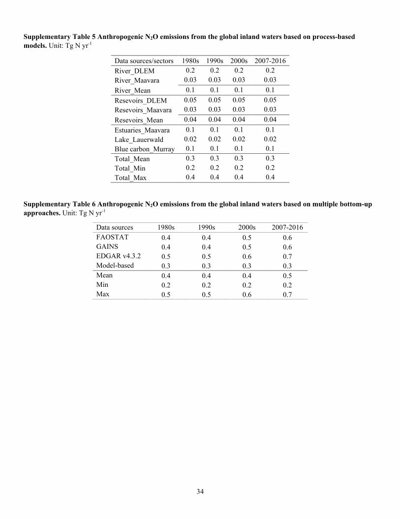
34

Supplementary Table 5 Anthropogenic N2O emissions from the global inland waters based on process-based models. Unit: Tg N yr-1

Data sources/sectors 1980s 1990s 2000s 2007-2016 River_DLEM 0.2 0.2 0.2 0.2 River_Maavara 0.03 0.03 0.03 0.03 River_Mean 0.1 0.1 0.1 0.1 Resevoirs_DLEM 0.05 0.05 0.05 0.05 Resevoirs_Maavara 0.03 0.03 0.03 0.03 Resevoirs_Mean 0.04 0.04 0.04 0.04 Estuaries_Maavara 0.1 0.1 0.1 0.1 Lake_Lauerwald 0.02 0.02 0.02 0.02 Blue carbon_Murray 0.1 0.1 0.1 0.1 Total_Mean 0.3 0.3 0.3 0.3 Total_Min 0.2 0.2 0.2 0.2 Total_Max 0.4 0.4 0.4 0.4

Supplementary Table 6 Anthropogenic N2O emissions from the global inland waters based on multiple bottom-up approaches. Unit: Tg N yr-1

Data sources 1980s 1990s 2000s 2007-2016 FAOSTAT 0.4 0.4 0.5 0.6 GAINS 0.4 0.4 0.5 0.6 EDGAR v4.3.2 0.5 0.5 0.6 0.7 Model-based 0.3 0.3 0.3 0.3 Mean 0.4 0.4 0.4 0.5 Min 0.2 0.2 0.2 0.2 Max 0.5 0.5 0.6 0.7

35

Supplementary Table 7 Natural N2O emissions from the global inland waters based on process-based models. Unit: Tg N yr-1

Data sources/sectors 1980s 1990s 2000s 2007-2016 River_DLEM 0.1 0.1 0.1 0.1 River_Maavara 0.02 0.02 0.02 0.02 River_Mean 0.04 0.04 0.04 0.04 Resevoirs_DLEM 0.04 0.04 0.04 0.04 Resevoirs_Maavara 0.03 0.03 0.03 0.03 Resevoirs_Mean 0.03 0.03 0.03 0.03 Estuaries_Maavara 0.05 0.05 0.05 0.05 Lake_Lauerwald 0.02 0.02 0.02 0.02 Blue carbon_Murray 0.2 0.2 0.2 0.2 Total_Mean 0.3 0.3 0.3 0.3 Total_Min 0.3 0.3 0.3 0.3 Total_Max 0.4 0.4 0.4 0.4

Supplementary Table 8 Nitrous oxide emissions due to atmospheric N deposition on land based on multiple bottom-up approaches. Unit: Tg N yr-1

Data sources 1980s 1990s 2000s 2007-2016 EDGAR v4.3.2 0.3 0.3 0.3 0.4 FAOSTAT 0.3 0.3 0.3 0.4 GAINS 0.3 0.3 0.3 0.4 FAOSTAT/EDGAR v4.3.2 0.6 0.6 0.7 0.8 GAINS/EDGAR v4.3.2 0.6 0.6 0.7 0.7 NMIP_Mean 0.6 0.7 0.8 0.8 NMIP_Min 0.3 0.4 0.4 0.4 NMIP_Max 1.2 1.4 1.3 1.4 Mean 0.6 0.7 0.7 0.8 Min 0.3 0.4 0.4 0.4 Max 1.2 1.4 1.3 1.4

36

Supplementary Table 9 Global N2O emissions from waste and waste water based on EDGAR v4.3.2 and GAINS estimates. Unit: Tg N yr-1

Data sources 1980s 1990s 2000s 2007-2016 EDGAR v4.3.2 0.1 0.2 0.2 0.2 GAINS 0.3 0.4 0.4 0.5 Mean 0.2 0.3 0.3 0.3 Min 0.1 0.2 0.2 0.2 Max 0.3 0.4 0.4 0.5

Supplementary Table 10 Global N2O emissions from fossil fuel and industry based on multiple bottom-up approaches. Unit: Tg N yr-1

Data sources Sectors 1980s 1990s 2000s 2007-2016

EDGAR v4.3.2

Energy 0.1 0.1 0.1 0.2 Transportation 0.2 0.2 0.2 0.2 Others_residential 0.1 0.2 0.2 0.2 Industry 0.7 0.5 0.5 0.5

GAINS Energy 0.3 0.4 0.5 0.5 Industry 0.5 0.5 0.4 0.3 Mean 0.9 0.9 0.9 1.0 Min 0.8 0.9 0.8 0.8 Max 1.1 1.0 1.0 1.1

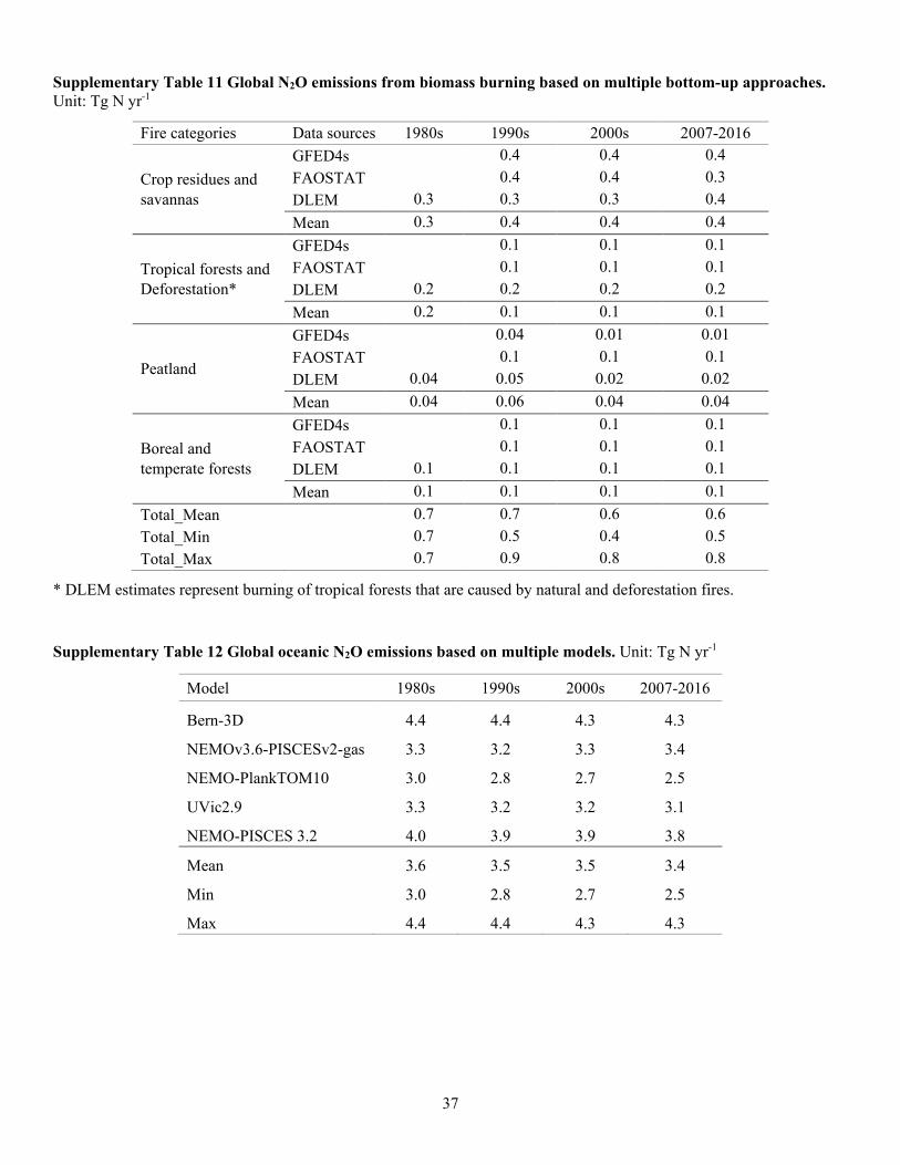
37

Supplementary Table 11 Global N2O emissions from biomass burning based on multiple bottom-up approaches. Unit: Tg N yr-1

Fire categories Data sources 1980s 1990s 2000s 2007-2016

Crop residues and savannas

GFED4s 0.4 0.4 0.4 FAOSTAT 0.4 0.4 0.3 DLEM 0.3 0.3 0.3 0.4 Mean 0.3 0.4 0.4 0.4

Tropical forests and Deforestation*

GFED4s 0.1 0.1 0.1 FAOSTAT 0.1 0.1 0.1 DLEM 0.2 0.2 0.2 0.2 Mean 0.2 0.1 0.1 0.1

Peatland

GFED4s

0.04 0.01 0.01 FAOSTAT

0.1 0.1 0.1

DLEM 0.04 0.05 0.02 0.02 Mean 0.04 0.06 0.04 0.04

Boreal and temperate forests

GFED4s

0.1 0.1 0.1 FAOSTAT

0.1 0.1 0.1

DLEM 0.1 0.1 0.1 0.1 Mean 0.1 0.1 0.1 0.1

Total_Mean 0.7 0.7 0.6 0.6 Total_Min 0.7 0.5 0.4 0.5 Total_Max 0.7 0.9 0.8 0.8

* DLEM estimates represent burning of tropical forests that are caused by natural and deforestation fires.

Supplementary Table 12 Global oceanic N2O emissions based on multiple models. Unit: Tg N yr-1

Model 1980s 1990s 2000s 2007-2016

Bern-3D 4.4 4.4 4.3 4.3

NEMOv3.6-PISCESv2-gas 3.3 3.2 3.3 3.4

NEMO-PlankTOM10 3.0 2.8 2.7 2.5

UVic2.9 3.3 3.2 3.2 3.1

NEMO-PISCES 3.2 4.0 3.9 3.9 3.8

Mean 3.6 3.5 3.5 3.4

Min 3.0 2.8 2.7 2.5

Max 4.4 4.4 4.3 4.3

38

Supplementary Table 13 Global N2O emissions based on multiple top-down approaches. Unit: Tg N yr-1

Name Category 2000s 2007-2016

INVICAT

Land

Ocean

Total

9.7

7.2

16.9

10.6

7.1

17.7

PyVAR-1

Land

Ocean

Total

9.4

6.4

15.8

10.6

6.4

17.0

PyVAR-2

Land

Ocean

Total

11.8

4.0

15.8

12.7

4.3

17.0

MIROC4-ACTM

Land

Ocean

Total

12.5

3.1

15.7

13.8

3.4

17.1

GEOSChem

Land

Ocean

Total

10.6

4.5

11.3

4.6

15.1 15.9

Mean

Land

Ocean

Total

10.8

5.1

15.9

11.8

5.1

16.9

Min

Land

Ocean

Total

9.4

3.1

15.1

10.6

3.4

15.9

Max

Land

Ocean

Total

12.5

7.2

16.9

13.8

7.1

17.7

39

Supplementary Table 14 Comparison of terminologies used in this study and previous reports.

GCP Terminology (in this study) IPCC AR5 (IPCC, 2013) National GHG inventories (used by UNFCCC according to IPCC, 2006 and IPCC, 2019)

UNFCCC / IPCC 2006 Source sector

Anthropogenic sources

Direct emissions of N additions in the agricultural sector (Agriculture)

Direct soil emissions (mineral N and manure fertilization, cultivation of organic soils, and crop residue returns) Agriculture

Direct N2O emissions from managed soils (except due to grazing animals)

3Da without 3Da3

Manure left on pasture Urine and dung deposited by grazing animals 3Da3 Manure management Manure management 3B Aquaculture --- --- ---

Other direct anthropogenic sources

Fossil fuel and industry Fossil fuel combustion and industrial processes Energy and industrial processes 1, 2

Waste and waste water Human excreta Waste 5 Biomass burning (from crop residue, grassland, shrubland and savannas; peat fires, tropical forests, boreal forests, and temperate forests)

Biomass and biofuel burning

Prescribed burning of savannas, field burning of agricultural residues 3E, 3F

Indirect emissions from anthropogenic N additions

Inland and coastal waters (rivers, lakes, reservoirs, estuaries, and coastal zones)

Rivers, estuaries, coastal zones Indirect emissions due to leaching and runoff 3Db2

Atmospheric N deposition on land Atmospheric deposition on land Indirect emissions due to atmospheric deposition

(of agricultural as well as other anthropogenic compounds emitted)

part of 3Db1

Atmospheric N deposition on ocean Atmospheric deposition on ocean part of 3Db1

Perturbed fluxes from climate/CO2/land cover change

CO2 effect --- --- --- Climate effect --- --- --- Post-deforestation pulse effect --- --- --- Long-term effect of reduced mature forest area --- --- ---

Natural sources and sinks

Natural soils baseline Soils under natural vegetation --- ---

Ocean baseline Oceans --- --- Natural (rivers, lakes, reservoirs, estuaries, and coastal upwelling) --- --- ---

Lightning and atmospheric production Lightning --- --- Atmospheric chemistry --- ---

Soil/wetland surface sink Surface sink --- ---

40

Supplementary Table 15 Comparison of the global N2O budget in this study with the IPCC AR5.

Note: ∗ Calculated from satellite observations combined with simple photolysis models in our study.

This study (2007–2016)

IPCC AR5 (2006/2011)

Bottom-up budget

Anthropogenic Sources Fossil fuel combustion and industry 1.0 (0.8–1.1) 0.7 (0.2–1.8) Agriculture (incl. Aquaculture) 3.8 (2.5–5.8) 4.1 (1.7–4.8) Biomass and biofuel burning 0.6 (0.5–0.8) 0.7 (0.2–1.0) Wastewater 0.3 (0.2–0.5) 0.2 (0.1–0.3) Rivers, estuaries, and coastal zones 0.5 (0.2–0.7) 0.6 (0.1–2.9) Atmospheric N deposition on ocean 0.1 (0.1–0.2) 0.2 (0.1–0.4) Atmospheric N deposition on land 0.8 (0.4–1.4) 0.4 (0.3–0.9) Other indirect effects from CO2, climate and land-use change 0.2 (-0.6–1.1)

Total Anthropogenic 7.3 (4.2–11.4) 6.9 (2.7–12.1)

Natural Sources and Sinks Rivers, estuaries, and coastal zones 0.3 (0.3–0.4) Oceans 3.4 (2.5–4.3) 3.8 (1.8–9.4) Soils under natural vegetation 5.6 (4.9–6.5) 6.6 (3.3–9.0) Atmospheric chemistry 0.4 (0.2–1.2) 0.6 (0.3–1.2) Surface sink -0.01 (0− -0.3) -0.01 (0− -1) Total natural 9.7 (8.0–12.0) 11.0 (5.4–18.6)

Total bottom-up source 17.0 (12.2–23.5) 17.9 (8.1–30.7) Observed growth rate 4.3 (3.8–4.8) 3.6 (3.5–3.8) Tropospheric sink 0.1 (0.1−0.2)

Stratospheric sink∗ 13.4 (12.3–14.4) 14.3 (4.3–28.7)

Atmospheric inversion Atmospheric loss 12.4 (11.7–13.3) 11.9 (11.0−12.8) Total source 16.9 (15.9–17.7) 15.8 (14.8−16.8)

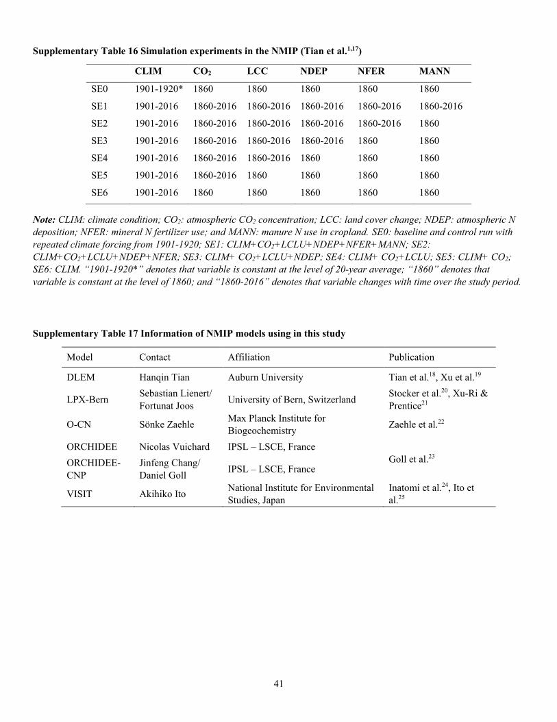
41

Supplementary Table 16 Simulation experiments in the NMIP (Tian et al.1,17)

CLIM CO2 LCC NDEP NFER MANN

SE0 1901-1920* 1860 1860 1860 1860 1860

SE1 1901-2016 1860-2016 1860-2016 1860-2016 1860-2016 1860-2016

SE2 1901-2016 1860-2016 1860-2016 1860-2016 1860-2016 1860

SE3 1901-2016 1860-2016 1860-2016 1860-2016 1860 1860

SE4 1901-2016 1860-2016 1860-2016 1860 1860 1860

SE5 1901-2016 1860-2016 1860 1860 1860 1860

SE6 1901-2016 1860 1860 1860 1860 1860

Note: CLIM: climate condition; CO2: atmospheric CO2 concentration; LCC: land cover change; NDEP: atmospheric N deposition; NFER: mineral N fertilizer use; and MANN: manure N use in cropland. SE0: baseline and control run with repeated climate forcing from 1901-1920; SE1: CLIM+CO2+LCLU+NDEP+NFER+MANN; SE2: CLIM+CO2+LCLU+NDEP+NFER; SE3: CLIM+ CO2+LCLU+NDEP; SE4: CLIM+ CO2+LCLU; SE5: CLIM+ CO2; SE6: CLIM. “1901-1920*” denotes that variable is constant at the level of 20-year average; “1860” denotes that variable is constant at the level of 1860; and “1860-2016” denotes that variable changes with time over the study period.

Supplementary Table 17 Information of NMIP models using in this study

Model Contact Affiliation Publication

DLEM Hanqin Tian Auburn University Tian et al.18, Xu et al.19

LPX-Bern Sebastian Lienert/ Fortunat Joos University of Bern, Switzerland Stocker et al.20, Xu-Ri &

Prentice21

O-CN Sönke Zaehle Max Planck Institute for Biogeochemistry Zaehle et al.22

ORCHIDEE Nicolas Vuichard IPSL – LSCE, France Goll et al.23 ORCHIDEE-

CNP Jinfeng Chang/ Daniel Goll IPSL – LSCE, France

VISIT Akihiko Ito National Institute for Environmental Studies, Japan

Inatomi et al.24, Ito et al.25

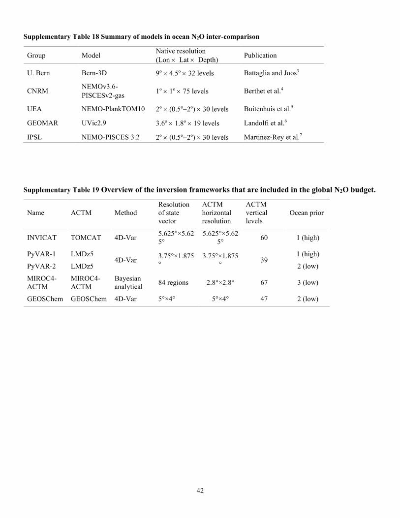
42

Supplementary Table 18 Summary of models in ocean N2O inter-comparison

Group Model Native resolution (Lon × Lat × Depth) Publication

U. Bern Bern-3D 9o × 4.5o × 32 levels Battaglia and Joos3

CNRM NEMOv3.6-PISCESv2-gas 1o × 1o × 75 levels Berthet et al.4

UEA NEMO-PlankTOM10 2o × (0.5o−2o) × 30 levels Buitenhuis et al.5

GEOMAR UVic2.9 3.6o × 1.8o × 19 levels Landolfi et al.6

IPSL NEMO-PISCES 3.2 2o × (0.5o−2o) × 30 levels Martinez-Rey et al.7

Supplementary Table 19 Overview of the inversion frameworks that are included in the global N2O budget.

Name ACTM Method Resolution of state vector

ACTM horizontal resolution

ACTM vertical levels

Ocean prior

INVICAT TOMCAT 4D-Var 5.625°×5.625°

5.625°×5.625° 60 1 (high)

PyVAR-1 LMDz5 4D-Var 3.75°×1.875

° 3.75°×1.875

° 39 1 (high)

PyVAR-2 LMDz5 2 (low)

MIROC4-ACTM

MIROC4-ACTM

Bayesian analytical 84 regions 2.8°×2.8° 67 3 (low)

GEOSChem GEOSChem 4D-Var 5°×4° 5°×4° 47 2 (low)

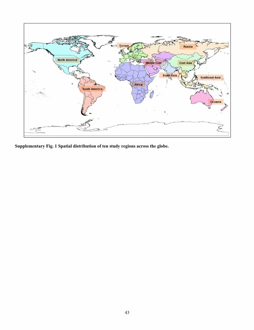
43

Supplementary Fig. 1 Spatial distribution of ten study regions across the globe.

44

Supplementary Fig. 2 Per capita N2O emission (kg N capita-1 yr-1) during 2007−2016. Annual population was obtained from FAOSTAT115 (http://www.fao.org/faostat/en/#data/OA).