Working Paper

A QUANTITATIVE GENERAL EQUILIBRIUM MODEL OF THE SWEDISH ECONOMY

I Lars Bergman and Andras Por

International Institute for Applied Systems Analysis A-2361 Laxenburg, Austria

NOT FOR QUOTATIGN WITHOUT PERMISSIGN OF THE AUTHOFi

A QUANTITATIVE GENERAL EQUILIBRIUM MODEL OF THE SWEDISH ECONOMY

L a r s Bergman a n d A n d r a s P o r

W o r l k i n g P a p e r s a r e i n t e r i m r e p o r t s o : ~ work o f t h e I n t e r n a t i o n a l I n s t i t u t e f o r A p p l i e d S y s t e m s A n a l y s i s a n d h a v e r e c e i v e d o n l y l i m i t e d r e v i e w . V i e w s o r o p i n i o n s e x p r e s s e d h e r e i n do n o t n e c e s s a r i l y r e p r e - s e n t t h o s e o f t h e I n s t i t u t e o r o f i t s N a t i o n a l Member O r g a n i z a t i o n s .

INTERNATIONAL INSTITUTE FOR APPLIED SYSTEMS ANALYSIS A-2361 L a x e n b u r g , A u s t r i a

PREFACE

A quantitative general equilibrium model is a useful tool primarily for two types of studies. One type is studies with a time horizon two or more decades into the future. In such studies, a model of this type can highlight various features of future economic conditions by delineating a number of resource allocations, each consistent with full equilibrium on product and factor markets. A second field of application is comparisons between actually observed resource allocations and hypothetical equilibrium allocations.

In this report a quantitative general equilibrium model of an open economy is developed and applied on Swedish data. In addition to the foreign trade flows, the model emphasizes the energy flows in the economy. The model is solved in a two-step procedure which is reiterated until a full equilibrium is reached. In the first step, technological coefficients and output prices are determined on the basis of initial values on factor prices. Then the excess demands on factor markets at product market equilibrium are determined. After that the initial factor prices are adjusted and the process repeated.

The report also contains some preliminary results, as well as a brief discussion of future directions of research in this field.

iii

CONTENTS

Introduction, 1

11. The Model, 2

11.1 Exogenous and endogenous variables, 3 11.2 Produced, consumed and traded commodities, 5 11.3 Technology and production costs, 6 11.4 Final demand, 9 11.5 Equilibrium conditions and the general level

of prices, 10 11.6 Definitions, 12 11.7 Some remarks about specialization and structured

damage in the model-economy, 13

111. The Solution Procedure, 15

IV. Some Preliminary Results, 20

IV. 1 The data base, 20 IV.2 An equilibrium allocation of resources in 1975, 23 IV.3 Some comparative statistics, 30

V. Some future directions of research, 32

References, 34

* INTRODUCTION

Nobody would deny that the basic conditions for economic activity in an industrialized national economy change a great deal over a period of two or three decades. The accumulation of net investments adds substantially to the economy's stock of real capital. The set of available production technologies is likely to change and this also applies to the supply and demand conditions on international markets for goods and services. Moreover, it is pos- sible that labor supply conditions will be quite different a couple of decades from now.

Much more.difficult to foresee is how and why these basic economic conditions change, and what these changes will mean in terms of, for instance, the material standard of living, employ- ment and energy consumption. Even if we regard the total capital stock, the technology and the labor force at some future point dn time as given magnitudes, a wide range of alternative resource allocations are possible. In addition, we may want to look at these resource allocations from many different points of view.

Among the possible resource allocations it seems to be reason- able to focus on one where all commodity and factor markets are cleared, and where there are no excess profits or losses in the production system; i.e. a situation consistent with general econo- mic equilibrium. This is not because such a situation is a very likely state of affairs; in fact it is probably a very unlikely situation in most industrialized economies. The reason is instead that a diseqilibrium will always produce forces, working through the market iaechanisil~ or throuqh the formation of economic policy, which tend to change the allocation of resources in the economy. Thus, a resource allocation which does not satisfy the basic

* Lars Bergman is responsible for Sections I, 11, IV, V, and Andras Por for Section 111.

equilibrium conditions mentioned above is a rather arbitrary description of the future state of an economy. An equilibrium allocation, on the other hand, is both feasible and can be main- tained under unchanged exogenous conditions. For this reason, a general equilibrium type of model seems to be a useful tool for characterizing economic conditions a couple of decades into the future.

Another way of utilizing a quantitative general equilibrium model is to compare a solution of the model with the actual situation in the economy at a given point in time. Such a com- parison indicates how close the actual allocation is to an e uilibrium allocation. The model can also highlight the nature 02 the disequilibrium situation, that is, give some rough indi- cations as to which sectors are ".too big" and which are "too small".

The purpose of this study is to develop and apply a model which can be used to calculate equilibrium resource allocations in a small, open economy under various assumptions about world market conditions and the domestic supply of primary factors of production. In this paper, the model is used for a comparison between the actual allocation of resources in the Swedish economy 1975 and an equilibrium allocation. Thus, we try to answer the question: to what extent was there a disequilibrium in the sectoral allocation of primary factors of production in Sweden 1975, and what was the macroeconomic significance of that disequilibrium ?

The paper is organized in the following way. In Section I1 the structure of the model is presented anddiscussed. Section 111 deals with the solution procedure while Section IV contains some preliminary results. Finally, in Section V, future directions of research are briefly discussed.

I1 THE MODEL

Given estimates of the total supply of labor and capital, world market conditions and production functions at some point in time, the model determines the sectoral allocation of labor and capital, This is done in such a way that all commodity and factor markets are simultaneously cleared. In this process the endogenously determined factor and commodity price system play a strategic role. Thus, except for the use of non-energy intermediate inputs, all technological coefficients are determined as functions of relative prices; that also applies to exports, imports and household expenditures. Public consumption expendi- tures and total net investment, on the other hand, are exogenously determined.

The model economy has one aggregated household sector and n+4 production sectors with sector index i = O,l, ..., n+3. In the applications presented in Section IV, n=20, but in general n can be any integer between 1 and N where N is determined by the ca- pacity of the available computer. There is only one kind of out- put from each of the production sectors, and each commodity is only produced in one sector. The sectors 0 and 1 are the energy

-

sectors, producing fuels and electricity respectively. Sector n+l is the housing sector and n+2 the public sector. The capital goods sector, n+3, is a book-keeping sector where various produced

goods are combined in fixed proportions. Thus, the input-output coefficients of the capital goods sector define the composition of the economy's stock of real capital.

The present model is an extended and elaborated version of a model previously developed by one of the authors (Bergman 1978) which, in turn, was inspired by earlier work by Johansen (1559 and 1974), Restad (1976) and Fdrsund (1977). It would lead too far to discuss all the differences between the present model and its predecessors, but the basic differences are related to the determination of foreign trade, domestic prices and the treatment of the energy sectors. In addition, the solution technique differs considerably from the one utilized by the above mentioned authors.

In the following presentation of the model, the exact form of production, household demand and foreign trade equations are specified. The parameters of these functions have been estimated in a rather crude way. Later on, when a more complete data base has been compiled, these parameters will be reestimated. Then it might also turn out that the functional forms should be revised. That will not change the basic features of the solution procedure presented in Section I11 provided the reestimated production func- tions are of a constant returns-to-scale type.

11. 1. Exoqenous and endoqenous variables

To begin with, the variables and parameters of the model are defined.

A. Endogenous variables

X j

gross output in sector j = 0,1 ..., n+3 j use of commodity i = 2,3, ..., n

Ki capital stock in sector j = 0,1, . . . , n+2 J

N i employment in sector j = 0,1, ..., n+2 ,J

Mi input of complementary imports* in sector j =0,1. J

'i household consumption of commodity i = 0,1, ..., n+l 'i export of commodity i = 1,2, . . . , n Mi import of commodity i=0,1, . . . , n 'i domestic production cost of commodity i = 0,1, . . . , n+3

2: domestic price of commodity i = 0,1,. . . , n+3

W index of the level of wages in the economy as a whole.

W j

wage rate in sector j = 0,1, ..., n+2 R index of the return on capital in the economy as a whole,

R j

net rate of return on casital in sector j =0,1, . . . , n+2

* j "user cost" of capital in sector j = 0,1, . . . , n+2

V - exchange rate (units of domestic currency per unit of foreign currency) .

*Complementary imports is meant to imply the import of commodities that cannot be (or at least are not) produced within the country.

0 household consumption expenditures.

Y real gross national product.

C total real household consumption.

Z total real exports

M total real imports

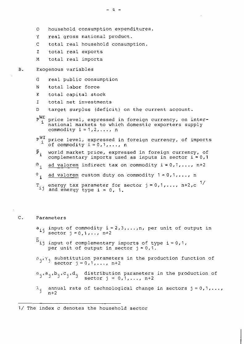
B. Exogenous variables

G real public consumption

N total labor force

K total capital stock

I total net investments

D target surplus (deficit) on the current account.

pWf price level, expressed in foreign currency, on inter- national markets to which domestic exporters supply commodity i = 1,2, ..., n

P? price level, expressed in foreign currency, of imports of commodity i=0,1, ..., n

- Pi world market price, expressed in foreign currency, of

complementary imports used as inputs in sector i=0,1

0 ad valorem indirect tax on commodity i=0,1, ..., n+2 i

ad valorem custom duty on commodity 1 = 0,1, ..., n i

T. energy tax parameter for sector j = 0,1, ..., n+2,c 1 / lj and energy type i = 0, 1.

C. Parameters

a input of commodity i=2,3 ,... ,n, per unit of output in ij sector j = 0, 1 , .. , n+2

iJ ij input of complementary imports of type i = 0,1, per unit of output in sector j =0,1.

pj,yj substitution parameters in the production function of sector j = 0,1, ..., n+2

ajfaj,b..c.,d distribution parameters in the production of j sector j = 0.1 ,. . . , n+2

X annual rate of technological change in sectors j = 0,1, ..., j n+2

-

1 / The index c denotes the household sector

' j annual rate of depreciation in sector j = 0,1, ..., n+2

0 annual rate of change of world market trade with com- j modity i=1,2, ..., n

w index of the relative wage rate in sector j =0,1, ..., j n+2

' j index of the relative rate of return on capital in sector j = 0,1, ..., n+2

'-ti, rlij expenditure and price elasticity paraneters in the household demand for commodity i = 0,1, ..., n+l

€idi price elasticity parameters in the export and import demand for commodity i = 0,1,. . . , n. l/ O O O constants in the production household demand, A.,Bi,Zi,X.,Mi

3 3 export and import functions.

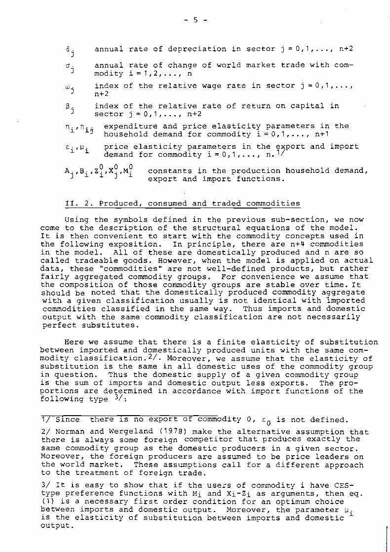
11. 2. Produced, consumed and traded commodities

Using the symbols defined in the previous sub-section, we now come to the description of the structural equations of the model. It is then convenient to start with the commodity concepts used in the following exposition. In principle, there are n+4 commodities in the model. All of these are domestically produced and n are so called tradeable goods. However, when the model is applied on actual data, these "commodities" are not well-defined products, but rather fairly aggregated commodity groups. For convenience we assume that the composition of those commodity groups are stable over time.It should be noted that the domestically produced commodity aggregate with a given classification usually .is~not identical with imported commodities classified in the same way. Thus imports and domestic output with the same commodity classification are not necessarily perfect substitutes.

Here we assume that there is a finite elasticity of substitution between imported and domestically produced units with the same com- modity classification.2/. Moreover, we assume that the elasticity of substitution is the same in all domestic uses of the commodity group in question. Thus the domestic supply of a given commodity group is the sum of imports and domestic output less exports. The pro- portions are determined in accordance with import functions of the following type 3 1 :

1/ Since there is no export ot commodity 0, E~ is not defined.

2/ Norman and Wergeland (1978) make the alternative assumption that there is always some foreign competitor that produces exactly the same commodity group as the domestic producers in a given sector. Moreover, the foreign producers are assumed to be price leaders on the world market. These assumptions call for a different approach to the treatment of foreign trade.

3/ It is easy to show that if the users of commodity i have CES- type preference functions with Mi and Xi-Zi as arguments, then eq. (1) is a necessary first order condition for an optimum choice between imports and domestic output. Moreover, the parameter pi is the elasticity of substitution between imports and domestic output.

Thus, there are three different commodity aggregates with index i : imported, domestically produced (and exported) and domestically consumed commodities of type i. Since the modelled economy is not assumed to be big enough to affect world market prices, these are taken as exogenously determined. The price of domestic output is determined by domestic production costs, while the price of domes- tically consumed units of commodity group i is determined in accordance with the following expression I / .

11. 3. Technolo~v and production costs

The production technology is characterized by constant returns to scale in all sectors. Labor, capital, fuel and electricity are substitutable factors of production, while the use of non-energy intermediate inputs is proportional to the level of gross output. The input of imported primary energy resources in the energy sectors is also proportional to the output levels in these sectors.

The description of the technology starts by the definition of a composite capital-labor input, Fj, and a composite fuel-electricity input, Hj, in accordance with the following equations:

Thus the elasticity of substituion between capital and labor is unity,while the elasticity of substitution between fuel and electricity is defined by (1 - yi)-1 where yi is a finite non-zero number different from unity. The composite factors of production Fj and Hj can be combined to yield gross output in accordance with

1

-.- DT 1/ For i=n+l,n+2 it nolds that Pi= Pi

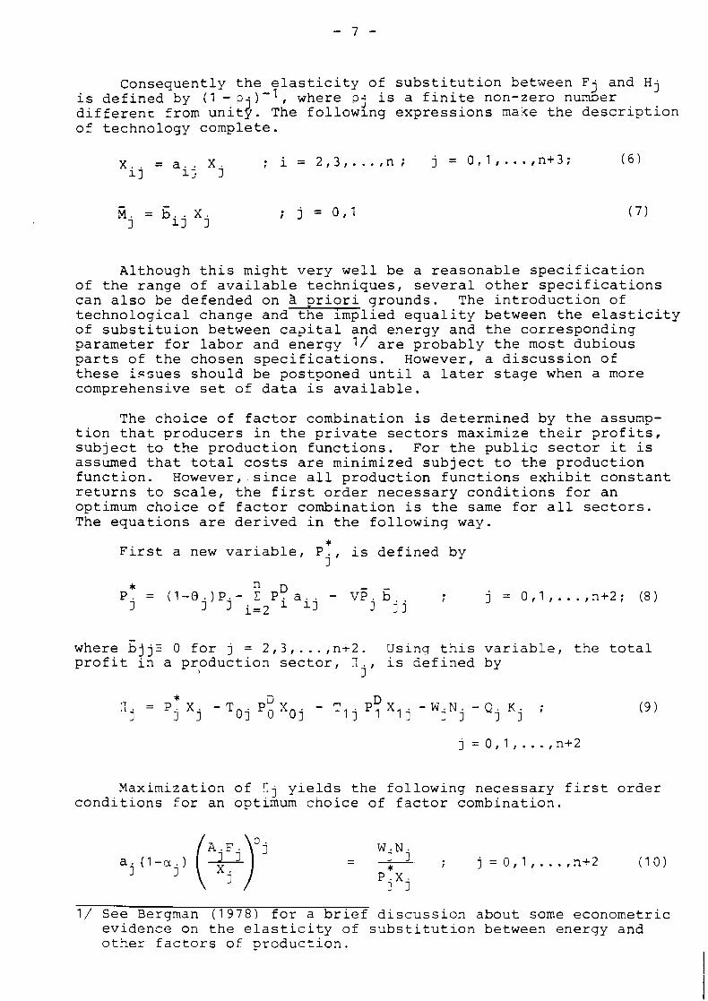
Consequently the elasticity of substitution between F and Hj is defined by (1 - pj)-l, where g j is a finite non-zero number different from unity. The following expressions make the description of technology complete.

Although this might very well be a reasonable specification of the range of available techniques, several other specifications can also be defended on a priori grounds. The introduction of technological change and the implied equality between the elasticity of substituion between cagital and energy and the corresponding parameter for labor and energy are probably the most dubious parts of the chosen specifications. However, a discussion of these issues should be postponed until a later stage when a more comprehensive set of data is available.

The choice of factor combination is determined by the assump- tion that producers in the private sectors maximize their profits, subject to the production functions. For the public sector it is assumed that total costs are minimized subject to the production function. However,.since all production functions exhibit constant returns to scale, the first order necessary conditions for an optimum choice of factor combination is the same for all sectors. The equations are derived in the following way.

* First a new variable, P is defined by

1,

where b j j ~ 0 for j = 2,3, . . . , nt2. Using this variable, the total profit in a production sector, 7 is defined by

b j'

Maximization of Cj yields the following necessary first order conditions for an optimum cnoice of factor combination.

1/ See Bergman (1978) for a brief discussion about some econometric evidence on the elasticity of substitution between energy and other factors of production.

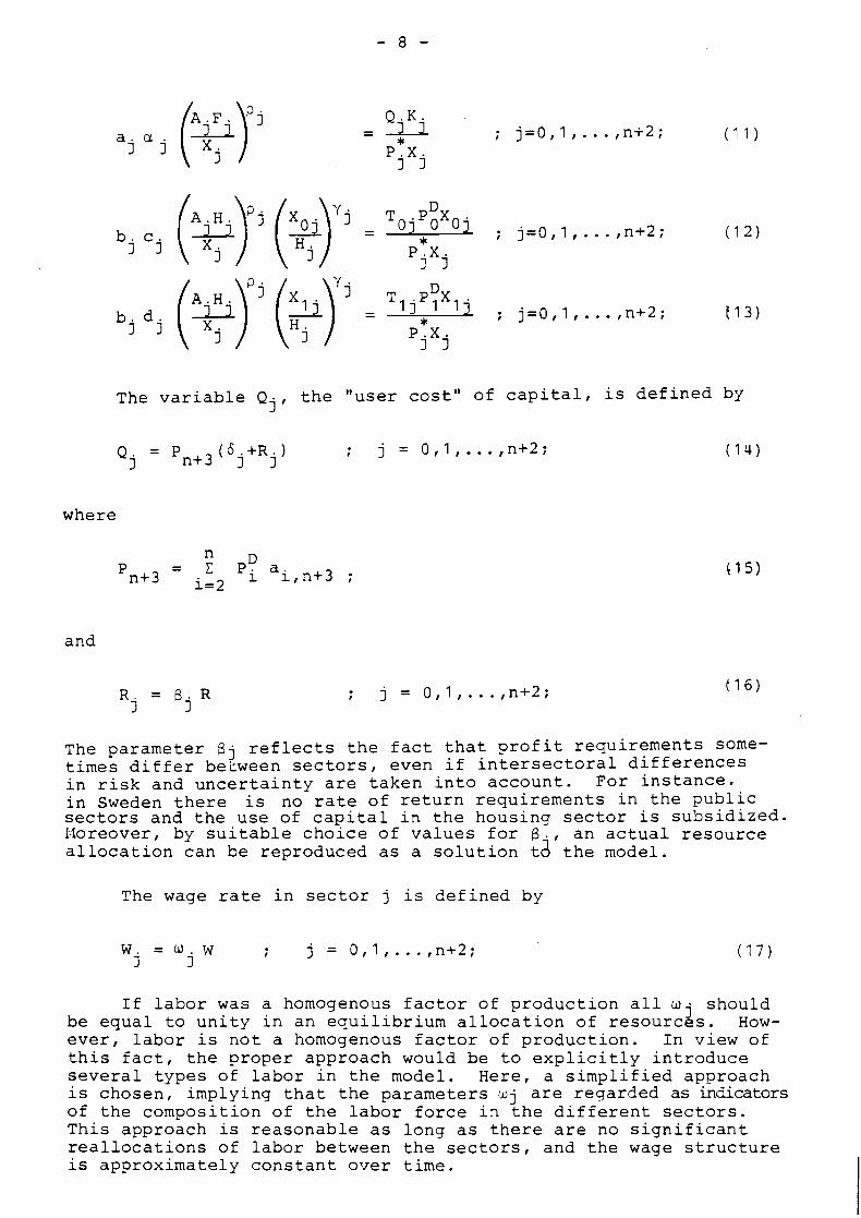
The v a r i a b l e Q j , t h e " u s e r c o s t ' o f c a p i t a l , i s d e f i n e d by

where

and

The p a r a m e t e r 3 j r e f l e c t s t h e f a c t t h a t p r o f i t r e q u i r e m e n t s some- t i m e s d i f f e r between s e c t o r s , e v e n i f i n t e r s e c t o r a l d i f f e r e n c e s i n r i s k and u n c e r t a i n t y a r e t a k e n i n t o a c c o u n t . F o r i n s t a n c e , i n Sweden t h e r e i s no r a t e o f r e t u r n r e q u i r e m e n t s i n t h e p u b l i c s e c t o r s and t h e u s e o f c a p i t a l i n t h e h o u s i n g s e c t o r i s s u b s i d i z e d . l ~ l o r e o v e r , by s u i t a b l e c h o i c e o f v a l u e s f o r B . , a n a c t u a l r e s o u r c e a l l o c a t i o n c a n b e r e p r o d u c e d a s a s o l u t i o n t d t h e model.

The wage r a t e i n s e c t o r j i s d e f i n e d by

I f l a b o r was a homogenous f a c t o r o f p r o d u c t i o n a l l w s h o u l d j b e e q u a l t o u n i t y i n a n e q u i l i b r i u m a l l o c a t i o n o f r e s o u r c e s . How- e v e r , l a b o r i s n o t a homogenous f a c t o r o f p r o d u c t i o n . I n v iew o f t h i s f a c t , t h e p r o p e r a p p r o a c h would b e t o e x p l i c i t l y i n t r o d u c e s e v e r a l t y p e s o f l a b o r i n t h e model . Here, a s i m p l i f i e d a p p r o a c h i s c h o s e n , i m p l y i n g t h a t t h e p a r a m e t e r s w j a r e r e g a r d e d a s indicators o f t h e c o m p o s i t i o n o f the l a b o r f o r c e i n t h e d i f f e r e n t s e c t o r s . T h i s a p p r o a c h i s r e a s o n a b l e a s l o n g a s t h e r e a r e no s i g n i f i c a n t r e a l l o c a t i o n s o f l a b o r be tween t h e s e c t o r s , and t h e wage s t r u c t u r e i s a p p r o x i m a t e l y c o n s t a n t o v e r t i m e .

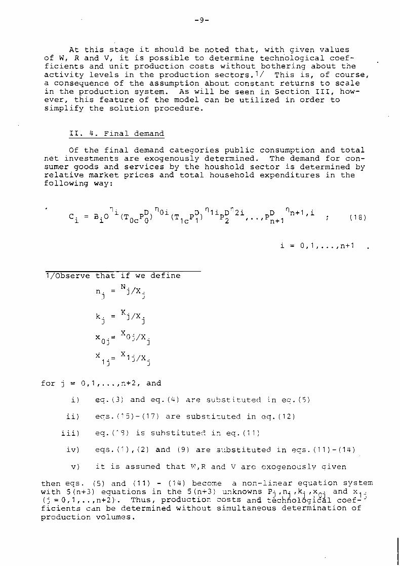
At this stage it should be noted that, with given values of W, R and V, it is possible to determine technological coef- ficients and unit production costs without bothering about the activity levels in the production sectors.l/ This is, of course, a consequence of the assumption about constant returns to scale in the production system. As will be seen in Section 111, how- ever, this feature of the model can be utilized in order to simplify the solution procedure.

11. 4. Final demand

Of the final demand categories public consumption and total net investments are exogenously determined. The demand for con- sumer goods and services by the houshold sector is determined by relative market prices and total household expenditures in the following way:

l/Observe that if we define

for j = 0, 1 , . . . ,n+2, and i) eq. (3) and eq. ( 4 ) are substituted in eo. (5)

ii) eqs. (15)- (17) are substituted in eq. (12)

iii) eq. (13) is substitute6 in eq. (1 1)

iv) eqs.(1),(2) and ( 9 ) are substituted. ineqs.(11)-(14)

v) it is assumed that V , R and V are exogenously qiven

then eqs. (5) and (1 1 ) - (1 4) become a non-linear equation system with 5 (n+3) equations in the 5 (n+3) unknowns P, ,-n, ,kj , xo j and x

1 j (1 =OI1..n+2). Thus, production costs and technological coef- ficients can be determined without simultaneous determination of production volumes.

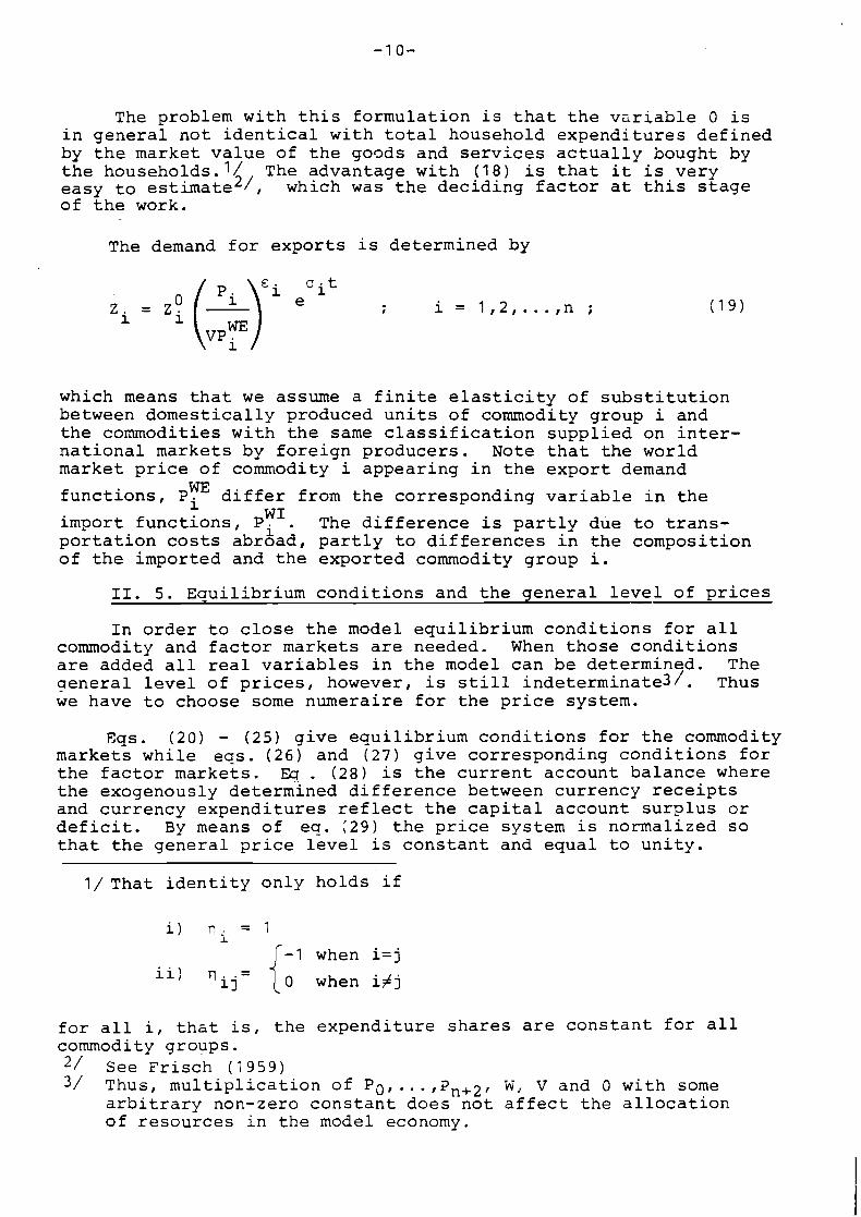
The problem with this formulation is that the variable 0 is in general not identical with total household expenditures defined by the market value of the goods and services actually bought by the households.l/ The advantage with (18) is that it is very easy to estimate2/, which was the deciding factor at this stage of the work.

The demand for exports is determined by

which means that we assume a finite elasticity of substitution between domestically produced units of commodity group i and the commodities with the same classification supplied on inter- national markets by foreign producers. Note that the world market price of commodity i appearing in the export demand

functions, PY differ from the corresponding variable in the WI import functions, Pi . The difference is partly due to trans-

portation costs abroad, partly to differences in the composition of the imported and the exported commodity group i.

11. 5. Equilibrium conditions and the general level of prices

In order to close the model equilibrium conditions for all commodity and factor markets are needed. When those conditions are added all real varLables in the model can be determined. The general level of prices, however, is still indeterminate31. Thus we have to choose some numeraire for the price system.

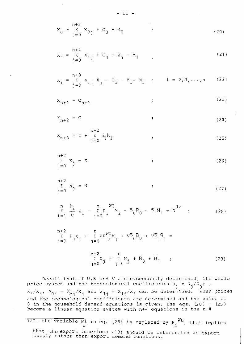
Eqs. (20) - (25) give equilibrium conditions for the commodity markets while eqs. (26) and (27) give corresponding conditions for the factor markets. Eq . (28) is the current account balance where the exogenously determined difference between currency receipts and currency expenditures reflect the capital account surplus or deficit. By means of eq. (29) the price system is normalized so that the general price level is constant and equal to unity.

I/ That identity only holds if

i) q i = 1

-1 when i=j ii) q i j 0 wheni#j

for all if that is, the expenditure shares are constant for all commodity groups. 2 / See Frisch (1959) 3 1 Thus, multiplication of PO, ...,P,+2f W, V and 0 with some

arbitrary non-zero constant does not affect the allocation of resources in the model economy.

n+3 - Xi - L a . . X + ci + zi- M ; i = 2,3, . . . , n

11 j i (22)

j=O

Recall that if W I R and V are exogenously determined, the whole price system and the technological coefficients n = N./X I I j ' k./X x . = X . / X i a n d x I jr 01 1 j = Xlj/xj

can be determined. When prices 01 -

and the technological coefficients are determined and the value of 0 in the nousehold demand equations is given, the eqs. (20 ) - (25 become a linear equation system with n+4 equations in the n+4

1/If the variable Pi in eq. (28) is replaced by piWE, that implies v

that the export functions (19) should be interpreted as export supply rather than export demand functions.

variables X U , j = O , l , ..., n+3. A solution to this system together with eqs. ( 3 6 ) - ( 2 9 ) yields measures of the, positix-e or negative. excess demands on the markets for capital, labor and foreign currency. This set of excess demands corresponds to the given values for R , W and V. By systematic revision of these values, a general equilibrium can be reached.

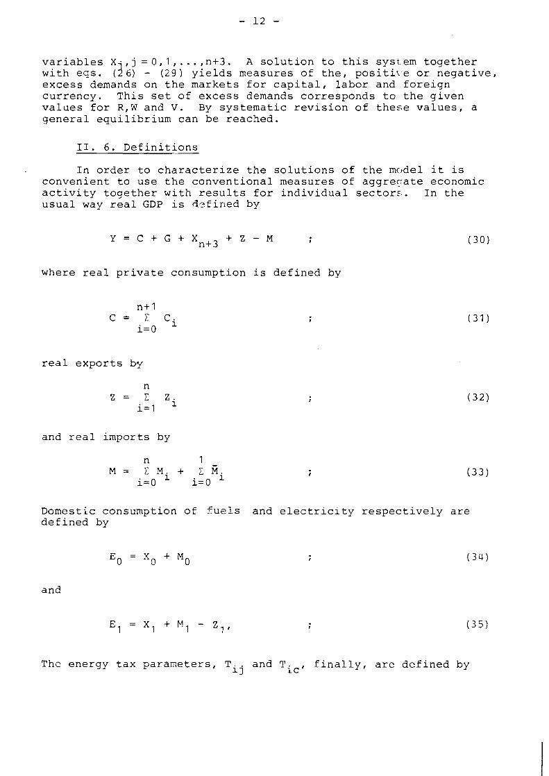
11. 6. Definitions

In order to characterize the solutions of the model it is convenient to use the conventional measures of agqre~~ate economic activity together with results for individual sectors. In the usual way real GDP is defined by

where real private consumption is defined by

real exports by

and real imports by

Domestic consumption of fuels and electricity respectively are defined by

and

El = XI + M I - Z1, I ( 3 5 )

The energy tax parameters, Tij and Tic, finally, are defined by

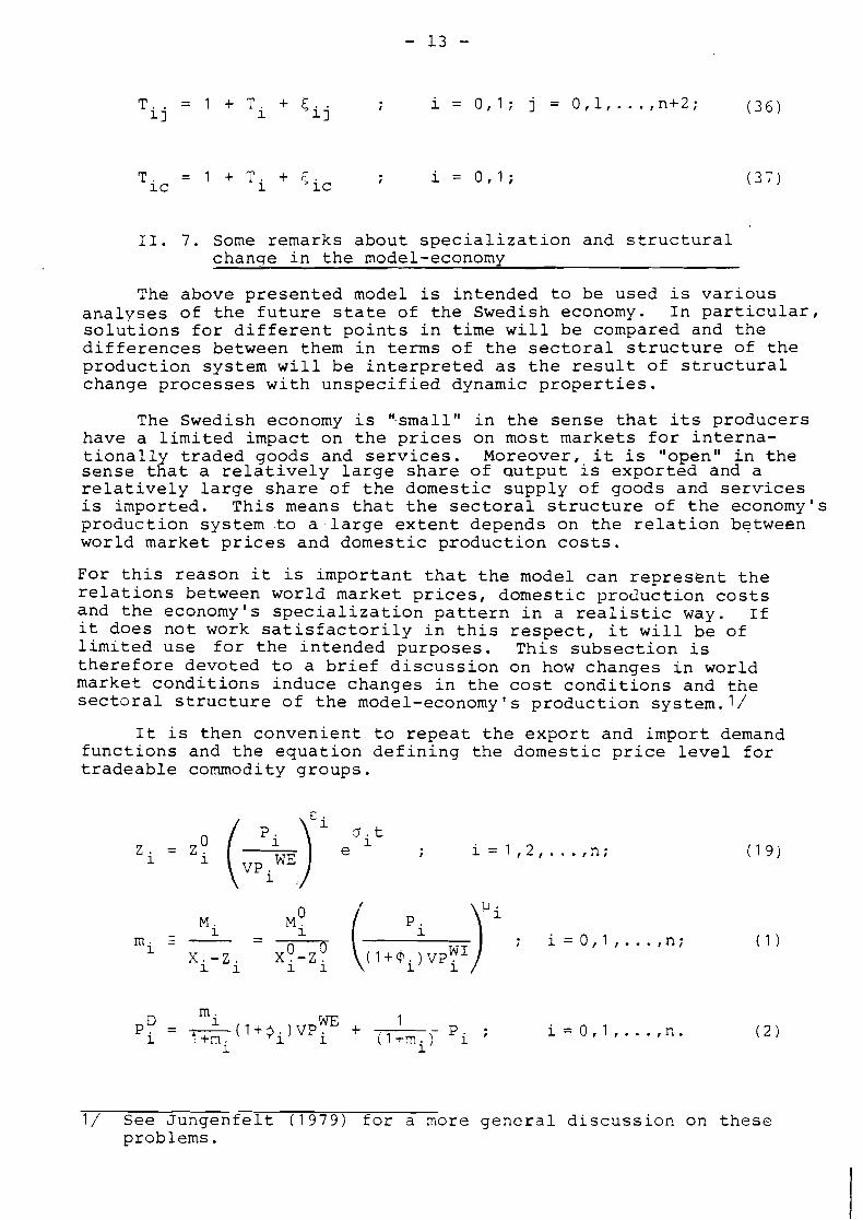
11. 7. Some remarks about specialization and structural change in the model-economy

The above presented model is intended to be used is various analyses of the future state of the Swedish economy. In particular, solutions for different points in time will be compared and the differences between them in terms of the sectoral structure of the production system will be interpreted as the result of structural change processes with unspecified dynamic properties.

The Swedish economy is small" in the sense that its producers have a limited impact on the prices on most markets for interna- tionally traded goods and services. Moreover, it is "open" in the sense that a relatively large share of ~utput is exported and a relatively large share of the domestic supply of goods and services is imported. This means that the sectoral structure of the economy's production system to a large extent depends on the relation between world market prices and domestic production costs.

For this reason it is important that the model can represent the relations between world market prices, domestic production costs and the economy's specialization pattern in a realistic way. If it does not work satisfactorily in this respect, it will be of limited use for the intended purposes. This subsection is therefore devoted to a brief discussion on how changes in world market conditions induce changes in the cost conditions and the sectoral structure of the model-economy's production system.l/

It is then convenient to repeat the export and import demand functions and the equation defining the domestic price level for tradeable commodity groups.

1/ See Jungenfelt (1979) for a more general discussion on these problems.

First, consider a case without aggregation over commodities. In such a case a distinction between domestically produced com- modities and the corresponding imported commodities cannot be maintained, provided transportation costs are properly taken into account. Thus, the absolute values of the parameters Ei and pi should approach infinity. This means that whenever the relative price variables in the foreign trade functions differ from unity, the set of tradeable goods can be partitioned into two subsets, one with the domestically produced and exported commodities and

. one with the imported commodities. The domestic commodity price system will coincide with world market prices expressed in the domestic currency unit. Moreover, in equilibrium the number of produced and exported tradeable goods will not be greater than the number of exogenously given factors of production, which is two in the present model. l/

It follows thatit is the assumptions that the parqmeters E~ and pi have finite values that prevents complete specialization in the model-economy. However, it is not an unreasonable assumption. In fact, in an empirical analysis it seems to be the-only reason- able assumption; even in very detailed commodity classification systems, commodities within the same cell on the most disaggre- gated level often exhibit differences in quality, etc.

Given that imported and domestically produced commodities with the same classification are not perfect substitutes, the equilibrium specialization pattern in the model-economy reflects international differences in unit production costs. As long as the domestic economy and "the rest of the world" grows at the same rate and cost conditions develop in a uniform way, the market shares of domestic producers on domestic and international markets remain unaffected. Thus, a price-cost equilibrium is maintained as long as there is a fixed relation between domestic production costs and world market prices. A ceteris paribus decrease in the world market price of an internationally traded commodity, or an increase in the domestic production cost for that commodity, will always result in decreased market shares at home and abroad for the domestic producers of the commodity in question.

However, this is not the whole story. If we continue to consider the case where the world market price of a given commodity decreases, it is clear from eq. (2) that the domestic price of that commodity will also decrease. This price decrease will work through the input-output system and result in lcwer production costs, and thus increase international competitiveness, in all domestic pro- duction sectors. This mechanism is reasonable and realistic, but unlike in the real world it is the only direct link between world market prices and domestic production costs in the model- economy at given factor prices. 21

In the real world there is an additional link between these two sets of variables, related to the zero or limited inter- sectoral mobility of real capital. At the planning, or ex ante, stage investments can be allocated between the sectors in accor- dance with profitability criteria. Once an investment is made,

1/~his is askandard result in international trade theory. 2/In order to attain an equilibrium, factor prices have to be ad- justed so that the exogenously given current account constraint can be satisfied.

the resulting capital equipment is %ore or less tied to the pro- duction unit in which the investment was made. Moreover, the ex post substitutability of the factors of production is usually lower than the corresponding ex ante figure.

Thus, if factor prices change over time and/or there is technological change, a production sector will at any point in time contain a set of production units representing a range of cost conditions at the prevailing factor prices. By a suitable ordering of the production units, the supply conditions of the sector can be described by an increasing supply curve. If the world market price of the commodities produced by a sector with these features is reduced, the demand for its output will, ceteris paribus, decrease. In the same way as in the model- economy the reduction of the sector's international competitiv- ness will be somewhat counteracted by reduced prices on inter- mediate inputs. In addition, it will be counteracted by a reduction of the sector's average production costs, as a direct result of the reduction of output. This is because it is the least efficient production units that will be closed down first when the world market price of the commoditygroup in question is re- duced. This mechanism is not incorporated in the constant returns to scale description of the production system in the present model.

To sum up, the model treats the impact of changes in world market conditions on the domestic allocation of resources in a realistic but somewhat incomplete way. The mechanisms that operate in the model-economy also operate in the real world, but not all mechanisms that operate in the real world are incorporated in the model. The consequence of this incompleteness of the model is that it tends to overestimate the impact of changes in world market con- ditions on the sectoral allocation of resources in the economy.This is because the lacking mechanism is one that dampens the impact on the sectoral structure rather than the opposite.

111. THE SOLUTION P?OCEDURE

In solving equilibrium models, one must find solutions for excess-demand equations in two sets of markets: commodity markets and factor markets. Various techniques have been developed tc solve such a system, but all are based essentially on one of two different approaches. The first approach is to reformulate the economic specification so that it can be treated as an optimization problem, which is then solved by means of mathematical programming methods. The second approach is to solve the equation system directly.

Within the general strategy of directly solving the system of nonlinear equations, we can further distinguish between two general approaches. The first is to reduce the problem to one of finding a fixed point of equations and then using a fixed point algorithm for numerical solutions. For example, the Scarf fixed point algorithm.l/ The other approach, which we have also partly taken, tries to attack the equation system in its

I / See Scarf ( 1973).

original form by using relatively simple nunerical techniques. For a survey of various methods within this approach, see Adelman and Robinson (1978).

Within the general strategy of directly attacking the equation system describing an equilibrium model, one has essentially a choice of two solution strategies. The first strategy is to solve for excess-demand equations in the factor markets and so sub- stitute out the commodity markets. This approach is called the

' factor-market strategy. This approach is efficient if the inner cycle of our numerical procedure for clearing the commodity market (including a price adjustment mechanism) is relatively sinple and the numberof factors is relatively smaller than the Lumber of commodities.

The second approach is to find the solution to the excess- demand equations in the commodity markets and so substitute out the factor markets. This approach is called the commodity-market strategy. In this approach one must first clear the factor markets in the inner cycle of the procedure and then clear the commodity -

markets in the outer cycle.

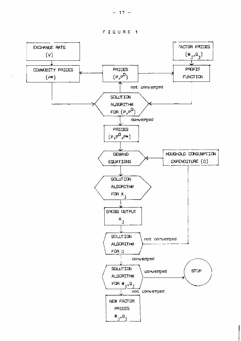
We have chosen the factor-market strategy F i g . . Our approach is to solve numerically the two equilibrium conditions in the factor markets (eqs. (26) and (27) ) as a function of factor prices We and Qj. As a subproblem, however, we must solve for market-clearing prices in the commodity markets with given factor prices Wj and Qj. Observe that all wage rates (Wj) depend only on the unknown W. Further, note that assuming prices are given, all "user-costsVof capital (Qj) depend only on unknown R. To equilib- riate conditions (26) and (27) in the factor markets, we have only to adjust variables W and R.

it is easy to see that our system is homogenous in exchange rate (V) and all prices. Therefore, we can fix unknown V to any reasonable value and solve the system for unique market-clearing prices in both markets. At the end of the solution procedure, the price system can be normalized by means of eq. (29) so that the general price level is constant and equal to unity.

We come now to the details of exactly how we derive the factor excess demands given initial values for variables W, R and V. We shall first consider the price adjustment mechanism and indicate how, given an initial set of variables W, R and V, we derive the prices p*, p and pD (Part I), then discuss com- modity demand and current account balance (Part 2) and finally, examine the excess-demand equation in the factor markets (Part 3 1 , along with the solution procedure.

EXCHANGE RATE

(v l

- 1 7 -

F I G U R E 1

I &

COMMOOITY PRICES 1 PRICES A

(+I (p,pD) FUNCTION I m

not converged

A L G W I T W

\ f

1 converged

d / DEMAND FH~OC-1

& SOLUTION

ALGORITHM

FOR X j

GROSS M P U T

I

i not covc rged - - - 1

\ FOR 0 / I 1 converged /'-1,

ALGORITHM

FWW. Q \ . J 9 j ) not converged 47 ( NEW FACTOR I

I PRICES I

P r i c e Adiustment: P a r t 1

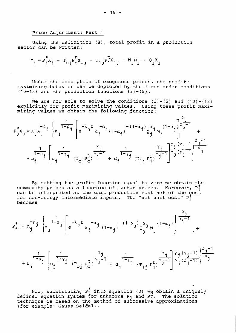
Using t h e d e f i n i t i o n (8), t o t a l p r o f i t i n a p r o d u c t i o n s e c t o r can be w r i t t e n :

Under t h e assumption o f exogenous p r i c e s , t h e p r o f i t - maximizing behav io r can be d e p i c t e d by t h e f i r s t o r d e r c o n d i t i o n s (10-13) and t h e p r o d u c t i o n f u n c t i o n s ( 3 ) - ( 5 ) .

W e are now a b l e t o s o l v e t h e c o n d i t i o n s ( 3 ) - ( 5 ) and ( 1 0 ) - ( 1 3 ) e x p l i c i t l y f o r p r o f i t maximizing v a l u e s . Using t h e s e p r o f i t maxi- mizing v a l u e s we o b t a i n t h e f o l l o w i n g f u n c t i o n :

By s e t t i n g t h e p r o f i t f u n c t i o n e q u a l t o z e r o w e o b t a i n t h e * commodity p r i c e s a s a f u n c t i o n o f f a c t o r p r i c e s . Moreover, Pj can be i n t e r p r e t e d a s t h e u n i t p r o d u c t i o n c o s t n e t o f t h e c o s t f o r non-energy i n t e r m e d i a t e i n p u t s . The " n e t u n i t c o s t " P: be comes

* Now, s u b s t i t u t i n g P a i n t o e q u a t i o n ( 8 ) we o b t a i n a un ique ly

d e f i n e d e q u a t i o n system $or unknowns P j and P ~ . The s o l u t i o n t echn ique i s based on t h e method of s u c c e s s i v d approximat ions ( f o r example: Gauss -Se ide l ) .

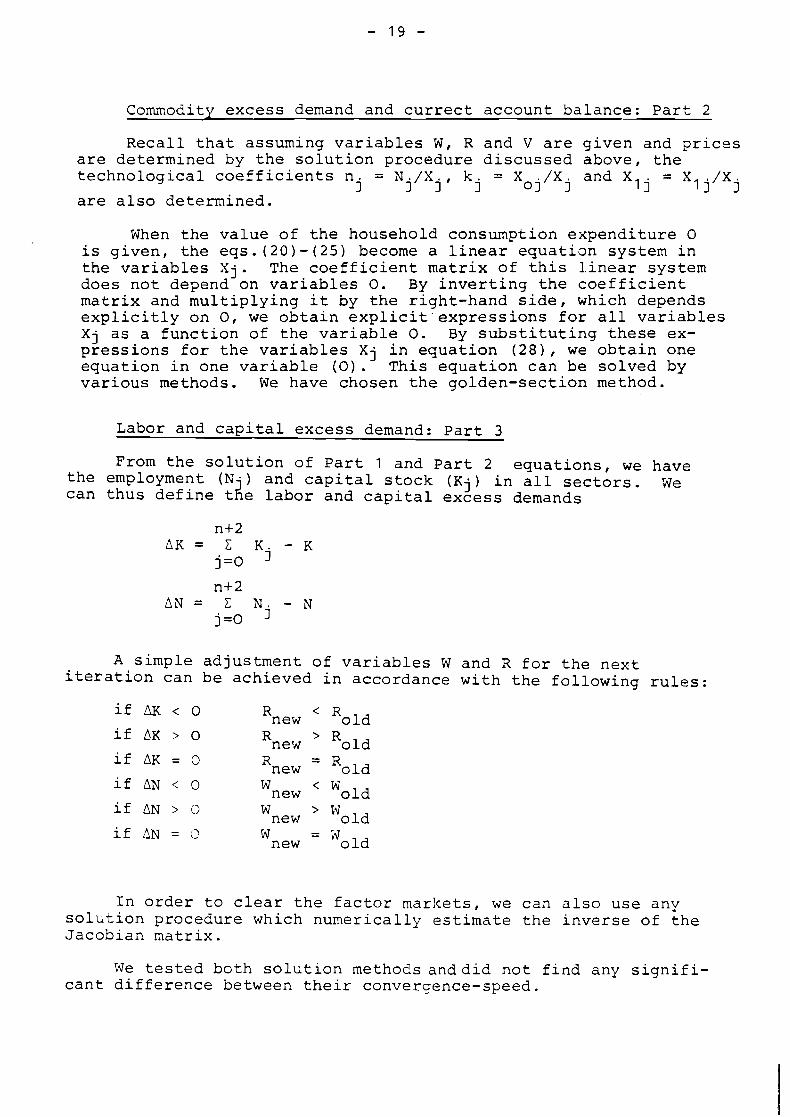
Commodity excess demand and currect account balance: Part 2

Recall that assuming variables W, R and V are given and prices are determined by the solution procedure discussed above, the technological coefficients n = N ./X k = X ./X and X = X ./X

j I jf j 01 j 1 j 1 1 j are also determined.

When the value of the household consumption expenditure 0 is given, the eqs.(20)-(25) become a linear equation system in the variables Xj. The coefficient matrix of this linear system does not depend on variables 0 . By inverting the coefficient matrix and multiplying it by the right-hand side, which depends explicitly on 0, we obtain explicit'expressions for all variables Xj as a function of the variable 0. By substituting these ex- pressions for the variables Xj in equation (28), we obtain one equation in one variable (0). This equation can be solved by various methods. We have chosen the golden-section method.

Labor and capital excess demand: Part 3

From the solution of Part 1 and Part 2 equations, we have the employment (N-) and capital stock (Kj) in all sectors. We can thus define tie labor and capital excess demands

A simple adjustment of variables W and R for the next iteration can be achieved in accordance with the following rules:

if AN > O W new > if AN = L1 W -

new - Wold

In order to clear the factor marlcets, we can also use any sol~tion procedure which numerically estimate the inverse of the Jacobian matrix.

We tested both solution metho2s anddid not find any signifi- cant difference between their convergence-speed.

IV. SOME PRELIMINARY RESULTS

In this section some preliminary results are prc.sented. After a brief discussion of the data base in sub-seciion IV.1, the following sub-section deals with a comparison of the actual allocation of resources in Sweden 1975 and an equilibrium allo- cation, as determined by the model. In sub-section IV.3 results from some comparative-statics experiments where the supply of capital and labor are varied, are presented. This means that, for the moment, we refrain from using the model for long term projection; instead we concentrate on computing equilibria under various conditions for a given point in time.

IV. 1. The data base

The bulk of the data base is obtained from an (unpublished) input-output table for Sweden. The data refers to the inter- sectoral flows in 1975.* The original table had 34 sectors, of which were industrial sectors. For this study some indus- trial sectors were disaggregated, while some nonindustrial sec- tors were aggregated. The resulting sectoral break-down can be seen in Table 1. The sectors 2-15 can be characterized as "industrial sectors." In addition the data base comprises estimates of the capital stock and the employment (measured in man-hours) in each of the production sectors. From this data the input coefficients for (non-energy) intermediate in- puts can be obtained from the input-output data. Moreover, given assumptions about the elasticity of substitution between types of energy and between energy and primary factors of production, and using the neoclassical theory of distribution, all the parameters of the production functions can be derived fror, the distribution data contained in the input-output table. Coupled with employment and capital stock data the same source can be used for derivation of the depreciation rates as well as the sector specific wage and profitability parameters (oj and Bj , respectively) .

The parameters of the household demand equations were ini- tially estimated in the way proposed by Frisch (1959). However, the fact that this type of demand system does not satisfy the budget constraint identically (see p.10) turned out to create problems; the comparative static analysis was disturbed by substantial variations in the error term.l/ For this reason it was simply assumed that all own-price elasticities were minus unity and all cross-price elasticities were equal to zero.

*The author is grateful to Mr. Bengt Rostr6nl at the Swedish Central Bureau of Statistics for providing the input-output data for this study. 1/By "error term" is meant the difference between the expendi- ture variable, 0, in the demand equations, and the market value of the consumer goods basket actually bought 5y the households, lpici. i

T a b l e 1 . The p r o d u c t i o n s e c t o r s .

Number

0 mergya/ 1 A g r i c u l t u r e , f i s h i n g , b a s i c f o o d

2 F o r e s t r y , wood, p u l p and p a p e r

3 Mining and q u a r r y i n g

4 O t h e r f o o d , b e v e r a g e s , l i q u o r a n d t o b a c c c ,

5 T e x t i l e , c l o t h i n g and l e a t h e r

6 P a p e r p r o d u c t s

7 C h e m i c a l

8 N o n - m e t a l l i c m i n e r a l p r o d u c t s e x c e p t p e t r o l e u m a n d c o a l

9 M e t a l s

10 F a b r i c a t e d m e t a l p r o d u c t s

1 1 N o n - e l e c t r i c a l m a c h i n e r y , i n s t r u m e n t s , p h o t o g r a p h i c a l

a n d o p t i c a l e q u i p m e n t a n d w a t c h e s 12 T r a n s p o r t e q u i p m e n t e x c e p t s h i p s and b o a t s

1 3 E l e c t r o t e c h n i c a l p r o d u c t s

1 4 S h i p y a r d s

1 5 P r i n t i n g and m i s c e l l a r ~ e o u s p r o d u c t s

1 6 H o t e l and r e s t a u r a n t s e r v i c e s , r e p a i r s , l e t t i n g o f

p r e r n i s e s o t h e r t h a n d w e l l i n q s , a n d p r i v a t e s e r v i c e s

o t h e r t h a n b a n k , i n s u r a n c e and b u s i n e s s s e r v i c e s

17 C o n s t r u c t i o n

18 W h o l e s a l e a n d r e t a i l t r a d t t , c o m m u n i c a t i o n s

19 T r a n s p o r t and s t o r a g e

20 F i n a n c i a l and i n s u r a n c e s e r v i c e s

2 1 Hous ing s e r v i c e s

22 P u b l i c s e r v i c e s

2 3 c / C a p i t a l goods-

a / I n t h i s s t u d y f u e l s and e l e c t r i c i t y a r e a g g r e g a t e d t o o n e s i n g l e - e n e r g y c o n n o d i t y . S e e p .

b / E x c l u d i n g p e t r o l e u m r e f i n e r i e s a n d a s p h a l t and c o a l p r o d u c t s . - c /The c a p i t a l g o o d s s e c t o r i s n o t a p r o d u c t i o n s e c t o r b u t a "book- -

k e e p i n g " s e c t o r wh ich a g g r e g a t e s d i f f e r e n t k i n d s o f c a ~ i t a l g o o d s , p r i m a r i l y m a c h i n e r y and b u i l d i n g s , i n f i x e d p r o p o r t i o n s t o a n a g g r e g a t e c a p i t a l good u s e d i n a l l " r e a l " p r o d u c t i o n s e c t o r s .

As was mentioned above (p.10) the budget constraint is satisfied identically in this case. In a later version of the model, the system of household demand equations will be replaced by a system with "better" properties.

The parameters in the import functions, i.e. the elasticities of substitution between imported and domestically produced com- modities with the same classification, was calculated on the basis of a study by Hamilton (1979). In that study import equa- tions of the same type as those in this study were estimated, but the commodity classifications in the two studies were not identical. Accordingly Hamilton's results could be used only after some aggregation and, in some cases, disaggregation. One can say that the estimates finally arrived at have some empirical ground, but very little can be said about the estimates in terms of conventional statistical criteria.

The export price elasticities were calculated on the basis of the impolrt price elasticities in accordance with the following reasoning: "If domestically produced and imported commodities with the same classification are substitutes on the Swedish market, that should also be the case on other national markets. Moreover, in view of the fact that Sweden primarily trades with other highly industrialized countries, the price elasticities in the export functions should not differ much from those in the import functions. However, since Swedish producers can be expected to have a relatively stronger position on the domestic than on the international market, the absolute values of the price elasticities should be somewhat lower in the import than in the export functions." The problem is, of course, to deter- mine the magnitude of "somewhat!'. This is obviously deep water, but some"guesstimation" was carried out, the result of which can be seen in Table 2.

As could be seen in the presentation of the model, it treats the demand for energy in a fairly elaborated way. For the moment we are not primarily concerned with energy demand, and in order to reduce the number of parameters to be estimated, fuels and electricity are aggregated into one single type of energy, pro- duced by an aggregated energy sector.

Formally this means that the variable H. in eq. (4) is re- placed by the aggregated energy input, made ap by fuels and elec- tricity in sector-specific fixed proportions. The elasticity of substitution between the aggregated energy input and primary factors of production was assumed to be .25 in all sectors.

This assumption is somewhat crude, but defendable on the basis of the econometric literature in this field. l/ Moreover, the assumption about the elasticity of substitution between energy and primary factors of production turned out to have an insignificant impact on sections.

the results presented in the following

Since we, at the moment, only are concerned with the situ- ation in 1975, we do not have to worry abo~t the time-dependent parameter^.^/ The data base contains estimates of all exogenous

1/See Bergr,an (1978) for a brief review. 2/That is, the rates of productivity increase and the growth of world market trade.

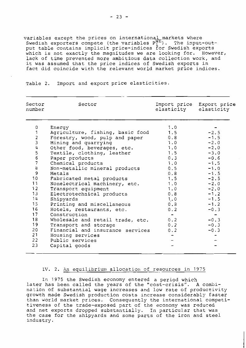
v a r i a b l e s e x c e p t t h e p r i c e s o n i n t e r n a t i o n a l m a r k e t s where Swedish e x p o r t e r s compete ( t h e v a r i a b l e s pYE) . The i n p u t - o u t - p u t t a b l e c o n t a i n s i m p l i c i t p r i c e - i n d i c e s f o r Swedish e x p o r t s which i s n o t e x a c t l y t h e m a g n i t u d e s w e a r e l o o k i n g f o r . However, l a c k o f time p r e v e n t e d more a m b i t f o u s d a t a c o l l e c t i o n work, and it was assumed t h a t t h e p r i c e i n d i c e s o f Swedish e x p o r t s i n f a c t d i d c o i n c i d e w i t h t h e r e l e v a n t w o r l d m a r k e t p r i c e i n d i c e s .

T a b l e 2 . Impor t and e x p o r t p r i c e e l a s t i c i t i e s .

S e c t o r number

S e c t o r Impor t p r i c e E x p o r t p r i c e e l a s t i c i t y e l a s t i c i t y

Energy A g r i c u l t u r e , f i s h i n g , b a s i c food F o r e s t r y , wood, p u l p and p a p e r Mining and q u a r r y i n g O t h e r f o o d , b e v e r a g e s , e t c . T e x t i l e , c l o t h i n g , l e a t h e r P a p e r p r o d u c t s Chemical p r o d u c t s N o n - m e t a l l i c m i n e r a l p r o d a c t s Metals F a b r i c a t e d m e t a l p r o d u c t s N o n e l e c t r i c a l m a c h i n e r y , e t c . T r a n s p o r t equ ipment E l e c t r o t e c h n i c a l p r o d u c t s S h i p y a r d s P r i n t i n g and m i s c e l l a n e o u s H o t e l s , r e s t a u r a n t s , e t c . C o n s t r u c t i o n Wholesa le and r e t a i l t r a d e , e t c . T r a n s p o r t and s t o r a g e F i n a n c i a l and i n s u r a n c e s e r v i c e s Housing s e r v i c e s P u b l i c s e r v i c e s C a p i t a l goods

-

I V . 2 . An e q u i l i b r i u m a l l o c a t i o n o f r e s o u r c e s i n 1 9 7 5

I n 1975 t h e Swedish economy e n t e r e d a p e r i o d which l a t e r h a s been c a l l e d t h e y e a r s o f t h e " c o s t - c r i s i s " . A combi- n a t i o n of s u b s t a n t i a l wage i n c r e a s e s and low r a t e o f p r o d u c t i v i t y g rowth made Swedish p r o d u c t i o n c o s t s i n c r e a s e c o n s i d e r a b l y f a s t e r t h a n wor ld m a r k e t p r i c e s . C o n s e q u e n t l y t h e i n t e r n a t i o n a l compet i - t i v e n e s s o f t h e t r a d e - e x p o s e d p a r t o f t h e economy was r e d u c e d and n e t e x p o r t s d r o p p e d s u b s t a n t i a l l y . I n p a r t i c u l a r t h a t was t h e c a s e f o r t h e s h i p y a r d s and some p a r t s of t h e i r o n a n d s t ee l i n d u s t r y .

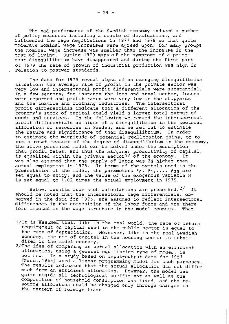
The bad performance of the Swedish economy induc:ed a number of policy measures including a couple of devaluations, and influenced the wage negotiations in 1977 and 1978 so that quite moderate nominal wage increases were agreed upon; for many groups the nominal wage increase was smaller than the increase in the cost of living. During 1979 many o f the symptoms of a price- cost disequilibrium have disappeared and during the first part of 1979 the rate of growth of industrial prodaction was high in relation to postwar standards.

The data for 1975 reveal signs of an emerging disequilibrium situation; the average rate of profit in the private sector was very low and intersectoral profit differentials were substantial. In a few sectors, for instance the iron and steel sector, losses were-reported and profit rates were very low in the shipyards and the textile and clothing industries. The intersectoral profit differentials indicate that a different allocation of the economy's stock of capital could yield a larger total output of goods and services. In the following we regard the intersectoral profit differentials as signs of a disequilibrium in the sectoral allocation of resources in Sweden, and we set out to estimate the nature and significance of that disequilibrium. In order to estimate the magnitude of potential reallocation gains, or to get a rough measure of the degree of disequilibrium in the economy, the above presented model can be solved under the assumption that profit rates, and thus the marginal productivity of capital, is equalized within the private sectorl/ of the economy. It was also assumed that the supply of labor was 2% higher than actual employment in 1975. In terms of the symbols used in the presentation of the model, the parameters 80, Bit..., f320 are set equal to unity, and the value of the exogenous variable N is set equal to 1.02 times the actual employment in 1975.

Below, results from such calculations are presented.2/ It should be noted that the intersectoral wage differentials, ob- served in the data for 1975, are assumed to reflect intersectoral differences in the composition of the labor force and are there- fore imposed on the wage structure in the model economy. That

1/It is assumed that, like in the real world, the race of return requirement on capital used in the public sector is equal to the rate of depreciation. Moreover, like in the real we dish economy, the use of capital in the housing sector is subsi- dized in the node1 economy.

2/The idea of comparing an actual allocation with an efficient allocation, using a general equilibrium type of model, is not new. In a study based on input-output data for 1957 Prierin, 19651 used a linear programming model for such purposes. The results indicated that the actual allocation did not differ inwh from an efficient allocation. However, the model was quite rigid; all technological coefficient as well as the composition of household consumption was fixed, and the re- source allocation could be changed only through changes in the pattern of foreign trade.

is, the observed values of the parameters w j are taken as given. In the same way the actual 1975 system of indirect taxes and subsidies is kept unchanged in the model calculations. However, the 1 9 7 5 data reveal a deficit on the current account but the model calculations are carried out under the assumption of a zero current account deficit.

Table 3 contains the results for some macro-economic variables as well as for factor prices and the exchange rate. According to these results an allocation where the marginal productivity of capital is equalized within the private sector of the economy and total employment is 2% higher than it was in 1975 would yield a 4 % largerGNP than the actual 1 9 7 5 allo- cation. Since public consumption and net investments are exogenously determined in the model and assumed to be equal to actual 1975 values, the incremental GNP is divided between household consumption and net exports. The division between these final demand componentsis such that the share of house- hold consumption in GNP is equal in both allocations.

Table 3. Actual and computed values for selected macroeconomic variables, factor prices and the exchange rate 1975 .

Actual value ~quilibrium value ( 2 ) : ( 1 ) ( 1 ( 2 ( 3 )

GNP * 2 7 8 . 9 Household consumption* 1 4 4 . 7 Industrial production* 2 3 4 . 3 Wage rate** 1 . O O Profit rate ( X ) * * * . 0 3 8 Exchange rate**** 1 . O O

*Expressed in l o 9 skr in actual purchasers' prices in 1975 . **Index of the wage level at a given sectoral wage structure. ***Net profits in the private sector in relation to the replace- ment value of the total capital stock in the private sector. ****Index. Domestic currency per unit of foreign currency.

It was mentioned above that the symptoms of a marked price- cost disequilibrium which became apparent during 1976 and 1977 induced devaluations of the Swedish currency and insignificant or negative real wage increases. The model results give some support for such a strategy; in comparison with an equilibrium allocation, wages were too high and the currency over valued. in Swede.2 already in 1975 .

According to these results it seems that the material stan- dard of living in Sweden in 1975 could have been significantly higher if the available real capital had been distributed over the production sectors in such a way that the marginal produc- tivity of capital had been equalized within the private sector of the economy. This conclusion also holds if the assumption that employment could be increased by 2% is relaxed. In that case, the increase in GTJP is, however, reduced to 2 . 5 % . It should also be noted that equalization of the marginal productivity

of labor in the economy, that is, relaxation of the assumption of a fixed wage structure, only led to a GKP-increase Sy a~proxi- mately 1 % . Moreover, variations in the assumption aboat the elas- ticity of substitution between energy and primary factors of production did not affect the results very much. Thcs, diffzrent sectoral allocations of capital seem to be the crucial difference between the actual and the equilibrium allocations.

However, there is an income distribution problem connected ' with the evaluation of the equilibrium allocation. As can be seen in Table 3, the more efficient allocation of the capital stock leads to a higher rate of' profit and at the saxe time a lower wage rate. Since factor supplies are given and constant, this means that the share of capital in the national income is considerably higher in the equilibrium allocation than in the actual allccation. Since capital incomes tend to be more un- evenly distributed than labor incomes, the equilibrium alloca- tion is not necessarily preferable to the actual allocation from a social welfare point of view.

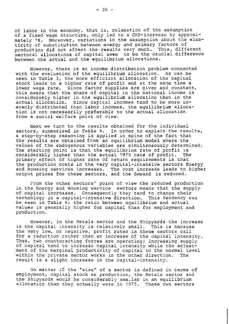
Next we turn to the results obtained for the individual sectors, summarized in Table 4. In order to explain the results, a step-by-step reasoning is applied in spite of the fact that the results are obtained from an equilibrium model where the values of the endogenous variables are simultaneously determined. The starting point is that the equilibrium rate of profit is considerably higher than the actual 1 9 7 5 rate of profit. The primary effect of higher rate of return requirements is that the production costs in the very capital-intensive sectors Energy and Housing services increases. The cost increase leads to higher output prices for these sectors, and the demand is reduced.

From the other sectors' point of view the reduced production in the Energy and Housing service sectors means that the supply of capital increases. Consequently they tend t.o change their technology in a capital-intensive direction. This tendency can be seen in Table 4; the ratio between equilibrium and actual values is generally higher for capital than for employment and product ion.

However, in the Metals sector and the Shipyards the increase in the capital intensity is relatively small. This is because the very low, or negative, profit rates in these sectors call for a reduction rather than an increase of the capital intensity. Thus, two counteracting forces are operating; increasing supply of capital tend to increase capital intensity while the adjust- ment of the marginal productivity of capital to the normal level within the private sector works in the other direction. The result is a slight increase in the capital-intensity.

No matter iE the "size" of a sector is defined in terms of employment, capital stock or production, the Netals sector and the Shipyards would be considerably smaller in an equilibrium allocation than they actually were in 7 9 7 5 . These two sectors

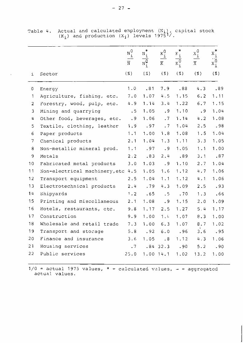
Table 4 . Actual and calculated employment (Ni) capital stock ( K ~ ) and production ( X j ) levels 1 9 7 5 1 ) .

i Sector

Energy 1 . 0 . 8 1 7 . 9 . 8 8 4 . 3 . 8 9

Agriculture, fishing, etc. 7 . 0 1 . 0 7 4 . 5 1 . 1 5 6 . 2 1 . 1 1

Forestry, wood, pulp, etc. 4 . 9 1 . 1 4 3 . 4 1 . 2 2 6 . 7 1 . 1 5

Mining and quarrying . 5 1 . 0 5 . 9 1 . 1 0 . 9 1 . 0 4

Other food, beverages, etc. . 9 1 . 0 6 . 7 1 . 1 4 4 . 2 1 . 0 8

Textile, clothing, leather 1 . 9 . 9 7 - 7 1 . 0 4 2 . 5 . 9 8

Paper products 1 . 1 1 . 0 0 1 . 8 1 . 0 8 1 . 5 1 . 0 4

Chemical products 2 . 1 1 . 0 4 1 . 3 1 . 1 1 3 . 3 1 . 0 5

Non-metallic mineral prod. 1 . 1 . 9 7 . 9 1 . 0 5 1 . 1 1 . 0 0

Metals 2 . 2 - 8 3 2 . 4 . 8 9 3 . 1 . 8 7

Fabricated metal products 3 . 0 1 . 0 3 . 9 1 - 1 0 2 . 7 1 . 0 4

Non-electrical machinery,etc 4 . 5 1 . 0 5 1 . 6 1 . 1 2 4 . 7 1 . 0 6

Transport equipment 2 . 5 1 . 0 4 1 . 1 1 . 1 2 4 . 1 1 . 0 6

Electrotechnical products 2 . 4 . 7 9 4 . 3 1 . 0 9 2 . 5 . 9 3

Shipyards 1 . 2 . 6 5 . 5 . 7 0 1 . 3 . 6 6

Printing and miscellaneous 2 . 1 1 . 0 8 . 9 1 . 1 5 2 . 0 1 . 0 9

Hotels, restaurants, etc. 9 . 8 1 . 1 7 2 . 5 1 . 2 7 5 . 4 1 . 1 7

Construction 9 . 9 1 . 0 0 1 . u 1 . 0 7 8 . 3 1 . 0 0

Wholesaleandretail trade 7 . 3 1 . 0 0 6 . 3 1 . 0 7 8 . 7 1 . 0 2

1 9 Transport and storage 5 . 8 . 9 2 6 . 0 . 9 6 3 . 6 - 9 5

20 Finance and insurance 3 . 6 1 . 0 5 . 8 1 . 1 2 4 . 3 1 . 0 6

21 Housing services . 7 - 8 4 3 2 . 3 - 9 0 5 . 2 - 9 0

22 Public services 2 5 . 0 1 - 0 0 1 4 . 1 1 . 0 2 1 3 . 2 1 - 0 0

~ -p -- - - - - - -- -- -- - - - - -

1 / 0 = actual 1 9 7 5 values, * - calculated values, - - - aggregated actual. values.

have in fact had great difficulties during the last few years and are now in a period of contraction. This result indicates that in spite of many far-reach3ng simplifications a.1~ weaknesses in its empirical basis, the model is able to elucidate some important aspects of reality.

However, Table 4 also contains some less satisf~ctory re- sults. Thus, the calculated production levels in Agriculture, Forestry and, to some extent, Mining and quarrying, are consider- ably higher than the corresponding actual values. S ~ n c e no sig- nificant expansion of these sectors has taken place since 1975, this result seems to be questionable.

In a narrow sense the reason is that the actual rates of profit in Agriculture and Forestry were quite high in 1975. Thus, in spite of the increase in the average rate of profit in the private sector, the profit rate equalization within that sector tends to reduce the rate of return requirement in Agri- culture and Forestry. Consequently, the production costs in these sectors tend to decrease, which, in turn, induce a demand expansion.

There is, however, reason to believe that the profit rates revzaled by the 1975 data are deficient for sectors highly de- pendent on natural resources. In these sectors there is a sub- stantial amount of land rents in total capital income, while the capital stock estimates refer to physical capital and neglect natural resources. Thus, the capital income and the capital stock measures are not compatible, and if land rents are not excluded from the capital income measure, the rate of profit will be overestimated. Since no such adjustment of the capital income data was made when the data base used in this study was prepared, we have probably seriously overestimated the actual 1975 profitability of the natural resource based sectors.

In Table 5 the results for domestic production costs, im- port prices expressed in the domestic currency unit and the do- mestic price level for each of the commodity groups can be seen. It should be noted that the corresponding actual 1975 values were all unity. The most marked differences between actual and calculated values are found for Energy, Metals, Housing services, Transport, Forestry, Hotels and restaurants and Finance. In the cases of Energy, and Housing services the basic reason is the high capital intensity in conjunction with substantially increased rate of return of capital, while the cost increase in the transkoyc sector partly depend on that factor, partly on the energy price increase. For the remaining of the somewhat extreme sectors, the major factor behind the production cost difference is the profit rate equalization within the private sector. 11 1/I:, Finance and insurance "unallocated bank services" were treated as capital income in the banking sector. This led to a very high profit rate for this sector in the data base.

T a b l e 5 . C a l c u l a t e d p r o d u c t i o n c o s t s , i m p o r t p r i c e s and d o m e s t i c p r i c e s f o r d i f f e r e n t commodity g r o u p s .

Commodity p roduced by s e c t o r

P r o d u c t i o n c o s t

I m p o r t Domes t i c p r i c e p r i c e

Energy

A g r i c u l t u r e , f i s h i n g , e t c .

F o r e s t r y , wood, p u l p , e t c .

Mining and q u a r r y i n g

O t h e r f o o d , b e v e r a g e s , e t c .

T e x t i l e s , c l o t h i n g , l e a t h e r

P a p e r p r o d u c t s

C h e ~ u i c a l p r o d u c t s

N o n - m e t a l l i c p r o d u c t s

M e t a l s

F a b r i c a t e d m e t a l p r o d u c t s

N o n - e l e c t r i c a l m a c h i n e r y , e t c .

T r a n s p o r t equ ipmen t

E l e c t r o t e c h n i c a l p r o d u c t s

S h i p y a r d s

P r i n t i n g and m i s c e l l a n e o u s

H o t e l s , r e s t a u r a n t s , e t c .

C o n s t r u c t i o n

Wholesa l e and r e t a i l t r a d e

T r a n s p o r t and s t o r a g e

F i n a n c e and i n s u r a n c e

Housing s e r v i c e s

P u b l i c s e r v i c e s

C a p i t a l goods

The results presented in Table 5 should also be inter2reted with an eye on the estimates, or the assumptions nade, of the price elasticity parameters in the import and export functions. If the ratio between the domestic cost and the import price is close to unity, the numerical value of the price-elasticity pa- rameter is fairly unimportant. The same applies for the corres- ponding parameter in the export functions when the relation between domestic production cost and the price, expressed in the domestic currency unit, on international markets where domestic exporters compete is close to unity. It should be noted that as a conse- quence of the assumptions made, import prices coincide with the prices charged by the domestic exporters' foreign competitors.

The results indicate that the price elasticity parameters are quite important in Forestry and Electrotechnical products. Together these sectors accounted for 21% of total exports and 9% of total imports in 1975, and the ratio between calculated production costs and world market prices (expressed in the do- mestic currency unit) is much different from unity. However, for several important foreign trade sectors, the import and export price elasticities are not that important. That is the case for Transport equipment (11% of exports, 8% of imports), Non-electrical machinery (17% of exports, 14% of imports) and Chemical products (6% of exports, 11% of imports).

It is quite obvious that the model gives a very simplified picture of the Swedish economy. Nevertheless it seems to be able to elucidate some important aspects of the.economic situation in 1975; an overvaluated currency, a somewhat too high wage level and too much resources tied to a couple of sectors with signifi- cantly reduced international competitiveness. Some of the results are dubious, but at least part of the problem can be overcome if land rents are treated in a more satisfactory way.

IV. 3. Some comparative statics

Clearly the assumptions made about the supply of capital and labor are quite strategic for the results obtained from the model. In order to indicate how sensitive the results are to these assumptions some comparative statics experiments were carried out. Thus, the assumptions about the supply of capital and labor were both varied +1C%. The resulting impact on GDP and relative factor prices can be seen in Diagrams 1 and 2. The diagrams indicate that the GDP-estimate is not very sensitive to the assumptions about capital snd labor; when the supply of capital or labor was varied between 90% and 110% of the original values, the GNP-estimate only varied between 93% and 107% of the value obtained in the solu- tion presei--ted in the preceding sub-section.

However, variations in the supply of capital and labor had a significant impact on relative, and to some extent also absolute, factor prices. These variations were'then reflected in the com- modity prices, but it was only for Energy and ~ousing services that the variations in capital and labor supply had a significant impact on production costs.

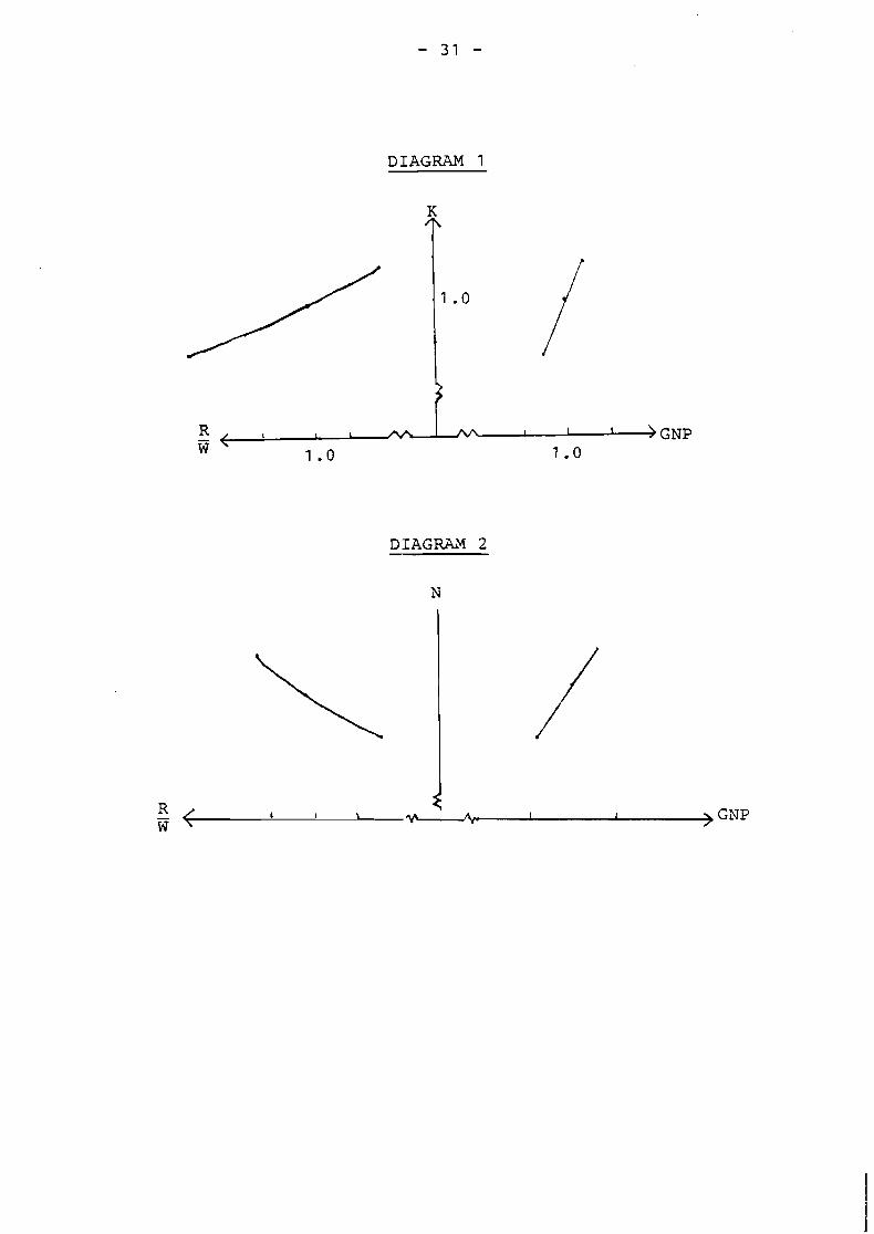
DIAGRAM 1

DIAGRAM 2

As was briefly mentioned in the preceding sub-section, the sensitivity of the solution with respect to the elasticity of substitution between energy and primary factors of ~roduction as well as to the wage-structure was investigated. In both cases the impact on GDP, private consumption and the sectoral structure was rather limited. Of course the elasticity of substitution between energy and primary factors of production turned out to be an important determinant of energy demand and thereby the size of the energy sector, but within reasonable limits the values of these parameters did not have a significant influence on the main features of the solution. In the same way, a complete wage equalization between the production sectors lead to increased production costs and reduced demand in some low-wage sectors, but again the main conclusians from the model simulation remained unaffected.

V. SOME FUTURE DIRECTIONS OF RESEACH

It seems reasonable to conclude that the model in its pre- sent version works satisfactorily, although a lot more work has to be put into the estimation of parameters. In that work it is quite possible that less restrictive functional forms for the description of technology and household demand will be chosen. The nested CES-Cobb-Douglas production functions used inthe pre- sent version imply a number of restrictions on the substitutability of various inputs. In light of empirical evidence these restric- tions might turn out to be unrealistic.

A rather attractive alternative approach to the specification of technology is to use cost rather than production functions. By using, for instance, a generalized Leontief cost functionl the restrictions on the elasticities of substitution, implied by the conventional production functions, can be relaxed.11 I-Iowever, it is reasonable to let the final choice of technology representation be determined by econometric considerations.

As was mentioned in connection with the presentation of the model, the fact that the constant-elasticity househcld demand equations do not satisfy the budget constraint led to problems which were overcome with some very heroic assumptions about the parameters in the equations. This is reason enough to replace the demand system with a system with "better" properties, but again the final choice of specification should be governed by econometric considerations.

More fundamental changes of the model would be related to the treatment of capital and capital formation. In the present version of the model, capital is malleable, and accordingly the model car, only highlight the properties of alternative long-run

'1 In a modern variant of the Norwegian MSG-model, focused on the energy flows in the economy, the production structure is represented by generalized Leontief cost functions. See

equilibrium allocations of a given amount of capital. However, in many cases one is interested in how the economy can move from a given short-run equilibrium, or even disequilibrium, to some kind of long-run equilibrium. A malleable capital model cannot say very much about such problems.

In order to improve the model in this respect, the capital stock should be regarded as tied to the sectors in which the investments were made. Moreover, a distinction between the ex ante and the ex post substitutability of inputs would also - represent an improvement of the model. Once such a development of the model is made, it is a natural step to distinguish between different vintages of capital, and to include investment functions and explicit intertemporal links. That would, however, require that sectoral investments are determined within the model. This can be done either by incorporating explicit investment functions for the production sectors, or by turning the model into an opti- mization model for determination of preferred multi-sectoral growth paths.

A methodology for estimating the properites of the production technology in such a way that ex ante and ex post elasticities of substitution can be distinguished has been developed by Fuss [1977]. In an extended version of the present model Fuss' approach could very well be incorporated. The basic econometric problem in the estimation of production structures with ex ante substitutability differing from ex post substitutability seems to be that explicit expressions for the formation of investors' expectations are required. In addition,the total capacity in the production sectors has to be decomposed into "vintages", and the use of inputs has to be assigned to these vintages. Such data is not easily available, and it thus seems that the practical problems connected with a more realistic treatment of capital are significant.

However, if a vintage capital approach could be implemented in a model with explicit intertemporal links, the treatment of the relation between world market prices, domestic production costs and structural change in the model would be considerably improved. (See the discussion on p 13f.). Moreover, with a model elaborated along these lines the comparison of actual and hypothetical equilibrium resource allocations would be focused on investments rather than the allocation of the entire capital stock. This means that results from calculations in the same spirit as those presented in this paper might become more useful from an economic policy point of view.

REFERENCES

Adelman, I. and S. Robinson (1978) Income Distribution Policy in Developing Countries: A Case Study of Korea. Published for the World Bank, Stanford University Press.

Bergman, L. (1978) Energy policy in a small open economy: The case of Sweden, RR-78-16 International Institute for Applied Systems Analysis, Laxenburg, Austria.

Frisch, R. (1959) A complete scheme for computing all direct and cross demand elasticities in a model with many sectors, Econornetrica 27:177-196.

Fuss, M.A. (1977) The structure of technology over time: A model for testing the putty-clay hypothesis. Econornetrica 45: 1797-1821.

F~rsund, F. (1977) Energipolitikk og ~konomisk vekst, DS I:16 Ministry of Industry, Stockholm, Sweden

Hamilton, C. (1979) Import penetration and import price elasticities with special reference to dynamic LIIC export commodities: The case of Sweden 1960-75. Seminar paper No.116, Institute for International Economic Studies, Stockholm, Sweden.

Johansen, L. (1959) A Multisectoral study of economic growth, North-Holland, Amsterdam, Holland.

Johansen, L. (1974) A multisectoral study of economic growth: Second enlarged edition, North-Zolland, Amsterdam, Holland.

Jungenfelt, K-G. (1979) Industrins strukturomvandling i en dppen ekonomi, Stockholm School of Economics (mimeographed).

Longva, S., Lorentsen, L. and 0. Olsen (1979) Energy in a multi- sectoral growth model, Research Department, Central Bureau of Statistics and the Norwegian Research Council (mimeo- graphed).

Norman, V. and T. Wergeland (1977) TOLMOD - a dual, general equilibrium model of the Norwegian economy, teknisk rapport, Senter for Anvendt Forskning, Norges Handelsh6yskole.

Restad, T. (1976) Modeller for sarnh~llsekonomisk planering, Liber FBrlag, Stockholm, Sweden.

Scarf, H. (1973) Computation of Economic Equilibrium, Newhaven, London, Yale University Press.

Werin, L. (1965) A Study of Production, Trade and Allocation, Uppsala.