Using Topography Statistics to Help Phase Unwrapping

A. Monti GuarnieriDipartimento di Elettronica e Informazione - Politecnico di Milano

Piazza Leonardo da Vinci, 32 - 20133 Milano - Italy

fax: +39-02-23993413, e-mail: monti@elet.polimi.it

Abstract

Conventional techniques approach Phase Unwrapping (PU) as an optimization problem, where figures of meritlike the total branch-cut length, the number of cuts, etc, is to be minimized. They disregard the properties of thefield to be unwrapped: the topography, i.e. the DEM, projected in the SAR reference. The purpose of the paper isto fill in this gap by providing statistics of the “fringe maps”. We first exploit the Woodward theorem to link theinterferogram Power Spectrum Density (PSD) with the Probability Density Function (PDF) of the Phase Gradientthat would result in a likely topography. A parametric model of the expected, unwrapped PG PDF is then derivedby exploiting the fractal properties of topography. Its parameters can be accurately estimated given the wrappedPG. This model provides useful statistic information for phase unwrapping. It is then possible, for example: (a)to estimate the number of residuals; (b) to find the best azimuth presumming factor and, (c), to find the optimalinterferogram range demodulation. Finally, we exploit the second order statistics of the PG field (as a fractal) toderive a suitable approximation for the expected length of the branch cuts.

Introduction

In this paper we provide hints in phase unwrapping intended mainly for DEM generation, where the final productis a medium resolution DEM, let us say sampled at 20 × 20 m. We will then refer mainly to the current and futurespace-borne SAR sensors like ERS, ENVISAT, TERRASAR, etc. An example of such interferometric systems isprovided in the simplified Interferometric SAR geometry of Fig. 2. As is widely known, an interferogram, like theone shown in Fig. 1 is achieved be taking the Hermitian product of the images acquired, either simultaneously bytwo sensors, or in by the same sensor in two repeat passes and properly coregistered [1, 2, 3, 4]. The phase of theinterferogram, shown in the figure, depends locally on the sensor-path distance: ψ(x, y) = 4π

λ

∣∣∣−−−−→S1 − P −−−−−→S2 − P

∣∣∣, andprovides information on the pixel elevation, hence the topography.

The generation of a Digital Elevation Model (DEM ) is then possible, on a pixel-by-pixel basis, provided that thephase ambiguity is solved. The aim of Phase Unwrapping (PU ) consists in recovering the integer number of cycles nto be added to the ambiguous, wrapped phase φ, to obtain the unambiguous phase ψ: ψ = φ+ 2πn, henceforth thepixel location. In a general case, where no a priori information on ψ is available, phase unwrapping is an ill-posedinverse problem: an infinite number of different solutions can be found, all honouring the data. The problem hasoriginated a very wide literature, where PU algorithms have been developed, basing on some a-priori assumptionsand trying to condition the problem in order to reconstruct a smooth phase field. A comprehensive summary of thesetechniques is provided in reference [5].

Even though some effort has been made to link the solution of PU to the properties of earth topography, [6], thespecific features of the actual signal to be unwrapped, i.e. the DEM projected in the SAR reference, are usuallyignored. As a matter of fact, any phase field is assumed ”reasonable”, provided that it is smooth [5].

This paper motivates from this assert, and shows how the properties of earth topography, that are known sinceearly fifties ([7], 1951), and more recently captured into statistics by Multi-Fractal Fields (MFF ) provides stringentconstraints in the solution of PU that would prevent ”any” smooth field to be a consistent solution.

This paper is based on the results achieved in reference [8], where it is shown that the MFF can be exploited toprovide a robust and quite accurate parametric model of the probability density of the unwrapped phase gradientin a SAR interferogram (PG-PDF ): these results are summarized in section 1. The model is then applied to phaseunwrapping by extending it to the realistic case of a noisy interferogram. Thereafter, it is shown how such model

1

can be exploited to estimate: (a) the density of singular points and, (b) the average cut length. This statistics are ofprimary importance in PU as they condition the solution. The role of the paper is to show that a proper PU shouldachieve an average number of singular points (and cut length) consistent with them local topography, opposite to thecommon assumptions that tends to minimize both cut length and residues. The force of the proposed approach reliesin the robustness of the parametric fractal model that provides an accurate estimate of unwrapped phase gradientstatistics even though the data explored are noisy and wrapped.

Finally, it is shown how two optimize two pre-processing steps, namely the interferogram flattening and multi-looking. In practice the multi-look factor and the flattening frequency are optimized to minimize the probabilityof aliasing that can be estimated basing on the fractal model. As a quite interesting result, it is shown that thenumber of singular points can be halved if the optimal flattening is exploited. Not surprisingly, it comes out that thisflattening imposes the most likely phase gradient to be different from zero in many cases of mountainous topography,or for large baselines.

Figure 1: Above: simulated interferogram of Mt. Vesuvius, by assuming ERS-ENVISAT geometry. Below: (left) theDEM used for the simulation, (right) the DEM can be approximated locally as a complex sinusoid.

A list of acronyms used throughout the whole paper is in table 1.

2

Figure 2: Simplified InSAR geometry.

3

Name DefinitionDEM Digital Elevation ModelInSAR Interferometric SARPRF Pulse Repetition FrequencyPDF Probability Density FunctionPG Phase GradientPSD Power Spectrum DensityPU Phase UnwrappingSNR Signal to Noise RatioUMF Universal Multi Fractal

Table 1: Acronyms and parameters adopted in the paper.

1 Ground slopes versus SAR PG

Our proposed approach is definitely to provides statistics information to PU that varies on a local scale: we mayexploit, for example, patches1 no larger than 10 × 10 km. Within such extent, we may well ignore the earth curvatureand assume parallel orbits, like in the simplified InSAR geometry of Fig. 2. We will ignore squint angles and assumeperfect yaw steering (ERS, ENVISAT etc). The figure introduces the definition of:

-the ground reference, used to define the topography, and identified by the coordinate (x, y) oriented with xparallel to the orbit (azimuth), and y cross-track (ground range),

- the SAR reference (x, r) where azimuth is parallel to the ground, that defines the space of the complex inter-ferogram,

- the ”normal baseline” Bn ' ∆θ/R0, i.e. the displacement of the two sensors normal to the view angle, wereθ, θ + ∆θ are the incidence angles of the two sensors.

We furthermore assume that, within the extents of a few pixels, the terrain slope is approximately constant, sothat we get a linear phase contribution to the complex interferogram, as shown in Fig. 1. The interferogram is then astationary frequency modulated process [9], whose local frequencies are related to the ground slopes by the followingexpressions (derived in [8]):

∆fx =∆φx

2π= − kBvsdx

sin θ − cos θdy(1)

∆fr =∆φr

2π= −hB

1 + dy tan θtan θ − dy

(2)

where kB =2f0c

Bn

R0and hB =

f0Bn

R0

where dx, dy are the two components of the height gradient. For such frequency modulated processes we can invokeWoodward’s theorem [10, 11], that links the interferogram PSD to the instantaneous frequencies PDF by:

S(∆f) = S(∆φ/ (2π)) ∝ f∆fx,∆fr(∆fx,∆fr) (3)

where ∆f and ∆φ represents the vectors of local frequencies and phase gradients.

1.1 Phase gradient probability distributions

Woodward theorem (3), can be exploited both in range and in azimuth to provide the PDF of the gradient as afunction ground slopes PDF. We recall here the expressions derived in reference [8].

1This approach is commonly adopted in literature (see for example [6]).

4

For the range case, the range frequency PDF is the following:

f∆fr (∆fr) = k1 + tan2 θ

(∆fr/hB − tan θ)2

· fdy(dy) |sin(θ − atan(dy)| (4)

where dy(∆fr) =1 + ∆fr/hB tan θ∆fr/hB − tan θ

k being a proportionality constant, computed by imposing unitary area. The range PG PDF is then obtained bythe linear transformation (2)

f∆φr (∆φr) = f∆fr

(∆φr

2π/fs

)fs

2π(5)

An example achieved by simulating an interferogram from a real DEM is provided in Fig. 3 that shows the PGhistogram, measured on the non-wrapped interferogram phase, and compared with the PDF of the ground slopesstretched by the transformation (4,5). The two plots fit quite well, except for the contributes layovered or shadowed(indeed a minor number of pixels in the image), that were not handled by the model (4).

-8 -7 -6 -5 -4 -3 -2 -1 0 1 210

-4

10-3

10-2

10-1

100

101

bn = 150 mbn = 200 mbn = 250 m

��

rgf ��

Range PG

Figure 3: Comparison between the range PG PDF, measured on a synthetic (non wrapped) interferograms phase(area of Naples) and its approximation, derived by transforming the range slope PDF.

5

The azimuth case is quite more complicated to handle, as the azimuth components of the slopes in the SARreference depend both on the along track and the across track slope on the ground. This is due to the foreshortening,that shifts an azimuth sloped terrain in the direction of the sensor (for ascending slopes). The azimuth frequencyPDF is the following:

f∆fx(∆fx) =∫fdx,dy (dx, dy) |sin θ − arctan dy| ·

· |dy(∆fx,W )− tan θ| dW (6)where W = kBvs cos θ (dy − tan θ)

This expression, like that of the range frequency PDF, needs to be computed numerically, basing on the 2D histogramof ground slopes, fdx,dy

(dx, dy). The azimuth PG PDF (non-wrapped) is obtained by applying a transformationidentical to (5).

1.2 Multi-Fractal Modelling

The capability of fractals in modelling topography is due to their feature of capturing the scale invariance of theheight gradient:

∆hnd=

(λ−n

)H ∆h0 (7)

where d= means equal in probability, H is constant, and λ−n is the resolution at which the gradient ∆h is measured.As the integer n increases, the scale λ−n gets finer and finer, however the gradient at that scale ∆hn = h(x +∆x/λ−n) − h(x) conserves its statistics, hence accounting for roughness in topography. This self-scaling, or selfsimilarity, is responsible of the power-law shape of the field PSD : Sε(f) ∝ f−β , already assessed by Kolmogorv inthe case of turbulence.

A generalization of such mono-fractals is provided by Multi-Fractal-Fields (MFF ), first introduced in [12], wherethe scale invariance property (7) is admitted to change its behaviour at different scales, or, in other words, thelogarithm of gradient PDF, log(Sε(f)) may have different slopes. Synthetic DEM can be generated by integratinga stocastic gradient, a MFF , as shown in Fig. 4. The MFF is supposed to be generated by a large numberof independent multiplicative stages (cascade process), each of them acting at a different scale. We expect, for thecentral limit theorem for products [10], that the MFF (see Fig. 4), is log-Normal distributed. Shertzer demonstratedthat the MFF PDF is log-Levy: a family of PDF that generalize the log-Normal one:

fh(h) = logLα,n,µ(h) (8)

=Lα,n,µ(x)|x=log h

hh > 0 (9)

Lα,n,µ(x) being the Levy PDF, whose characteristic function is known in closed form expression [13]:

L(ω) = exp(−n |ω|α exp

(j1− |1− α|

4sign(ω)

))· (10)

· exp(jωµ), 0 ≤ α ≤ 2, n ≥ 0

The close resemblance between a MFF and the topographic height gradient leads to the assumption that this lastis log-Levy distributed [14]:.

f|d|(∆h) = logLα,n,µ(∆h)

It is shown in [8] that this is indeed the case, and the link between the parameters α, n, µ and the local topographyis discussed there.

1.3 Ground slopes PDF

The MFF model of gradient has been exploited to derive the model of the PG-PDF in range and azimuth in [8].

6

Figure 4: Universal Multi Fractal Field (above), and the result after fractional integration (below). This stochasticfractal provides a realistic DEM resemblance.

7

The distribution of ground slopes along any direction, e.g. the projection of the gradient on the generic axis:d = |d| cos θ, has been derived in [8]:

fd(d) =∫ ∞

|d|logLα,n,µ(y)

1

π√y2 − d2

dy (11)

This expression is to be used in (4) for modelling range PG-PDF, just e.g. by inserting (11) into (4).

The azimuth PG-PDF, in (6) requires the 2D PDF of ground terrain slopes, (see [8]):

fdx,dy(dx, dy) = logLα,n,µ

(√d2

x + d2y

) √d2

x + d2y

2π(12)

1.4 Parametric model for PG-PDF

The expressions (4,6) of the PG PDF need to be combined with the fractal models of terrain slopes, (11, 12) toprovide a parametric model of PG PDF. The simplest way to estimate the values of the parameters involved: (α, n, µ),is just by imposing a fit of the model with the estimated interferogram PSD, i.e. the Woodward theorem (3) asdiscussed in [8]. As an example, Fig 7 plots the PG PDF retrieved by a (wrapped) synthetic interferogram andcompared with the true one, estimated by the known unwrapped fringes (area of Mt. Vesuvius).

It is quite important to stress the fact that the interferogram PSD is known up to the Nyquist frequency (withsome alias), whereas the parametric model is capable to predict the probability of unwrapped PG values. Thecapability of the model to fit the real case for a very wide dynamic range is essential for the application proposed,since the error probabilities are influenced by the tails of the distributions shown in the figure.

2 Phase unwrapping

Let us come back to the PU problem already introduced: we need to recover the integer number of cycles n to beadded to the wrapped phase φ to get the unambiguous phase value ψ: ψ = φ + 2π · n. We already stated that,in absence of a priori information about φ, we get an ill-posed inverse problem (infinite solutions). Almost all thePU algorithms assume smooth phases, hence the neighbouring the uwrapped field is supposed to varies less than πradians form one pixel to another. Though this hypothesis is often valid for most of the image pixels, the presenceof phase discontinuities (i.e. absolute phase variations between neighbouring pixels greater than π radians) preventsone from using the most straightforward PU procedure: a simple integration of the phase differences, starting froma reference point. In fact, phase discontinuities generate inconsistencies, since integration yields different resultsdepending on the path followed. This feature is evident whenever the sum of the wrapped phase differences (theintegral of the estimated phase gradient) around a closed path differs from zero. To be consistent a gradient fieldmust be irrotational; i.e. the curl of ∇φ should be zero everywhere [5]. Whenever this condition is verified all overthe interferogram we face the “trivial PU problem”. Unfortunately, this is never the case in InSAR data processing.

The rotational component of the gradient field can be easily estimated summing the wrapped phase differencesaround the closed paths formed by each mutually neighbouring set of four pixels. Whenever the sum is not zero aresidue is said to occur [1]. Its value is usually normalized to one cycle and it can be either positive (+1) or negative(-1). The summation of the wrapped phase variations along an arbitrary closed path equals the algebraic sum of theresidues enclosed in the path. An example is provided in Fig.5: notice that the residues, marked in Fig. 5.c, markthe endpoints of the “discontinuities lines”.

The true problem is then their complete identification. Discontinuities are essentially due to two independentfactors: (1) phase noise; (2) steep terrain slopes. In Fig. 5, only a pair of residues is due to ”topography”, whereas allthe other, due to noise, are quite distinguishable are they are close together. The most demanding problem in phaseunwrapping is to find out the correct ”ghost line” that connect each pair of residues. In usual phase unwrappingscheme, different strategies have been followed and different algorithms have been developed. In practice, almost allPU algorithms seek to minimize the following cost function:

8

Figure 5: Residues due to noise and phase unwrapping. The pyramid in (a) has been converted into wrapped phases,and then noise was superimposed. The resulting interferogram has then been filtered, giving the phases in (b). Theresidues have then been identified and marked as black / white pixels in (c) (depending on the sign). The sole tworesidues due to topography are evidenced by arrows, all the other residues are due to noise and appear in close pairs(one of these pairs has been marked by a white circle).

9

C =∑i,j

w(r)i,j

∣∣∣∆(r)ψi,j −∆(r)w φi,j

∣∣∣p (13)

+∑i,j

w(a)i,j

∣∣∣∆(a)ψij −∆(a)w φi,j

∣∣∣pwhere 0≤p≤2, ∆ indicates discrete differentiation along range (r) and (a) azimuth direction respectively, w

are user-defined weights and the summations including all appropriate rows i and column j. The suffix w to thedifferentiation operator ∆ indicates that the phase differences are wrapped in the interval +π−π.

We stress that this objective function has not been obtained from a theoretical analysis or a statistical descriptionof a topographic phase signal in SAR coordinates. It is just a reasonable translation in mathematical terms of ourbasic assumption: ∆ψ = ∆wφ almost everywhere.

2.1 Phase unwrapping and topography statistics

The fundamental expression (13) turns the PU problem into an optimization problem, where the cost to minimized(C), can be either the total length of ghost lines (norm p = 0), or the total ”charge”, amount of 2π (norm p=1). Inthis sense, it is common assumption in PU that several solutions can be obtained, all consistent with the wrappeddata, and, apparently none of them ”better” than the other. We will show here that this assumption is untrue, asthe local topography constraints the admissible solution. In particular, we will derive here: (1) the total number ofresiduals, and (2) the expected length of ghost lines. None of these two figures is to be minimized at any cost, butrather dimensioned according to the ”fractal” parameters.

As an example, Fig. 6 shows the residues in an interferogram simulated by exploiting a DEM of Mt. Etna, andthe correct location of the ghost lines. In a ”blind” PU approach, like the one derived from (13), the correct solutionwould not be found as it does not minimize the total cut length, nor the total charge.

Figure 6: (Left): the circles mark residues (or group of residues) measured on an interferogram simulated form thetrue DEM of Mt. Etna. (Right): the correct location of the ghost lines, as would appear on the unwrapped phase.The correct direction and length of ghost lines can be found only by accounting for topography statistics.

Let us first compute the occurrence of residues in the noiseless case, e.g. in presence of topographic effects only.We need to compute the probability:

P (|∆φ−∆φf | > π) or (14)P (∆φ−∆φf > π) + P (∆φ−∆φf < −π)

by integrating the PG-PDF: (5) for azimuth and (4) for range. The term ∆φf , in (14), have been inserted toaccount for the proper ”flattening”, in range direction, that will be discussed later: we may assume here that ∆φf

corresponds to the PG of flat terrain. An example of the PG-PDF is shown in Fig. 7, that compares the histogram ofthe unwrapped phase gradient, achieved by exploiting the DEM of Mt. Vesuvius, and the model fitted by exploitinga highly correlated interferogram (may be multi-look averaged). The model is enough robust to provide a good fit ofthe histogram tails, hence an estimate of the aliasing probability (the shaded areas in the figure). This area providesthe number of residuals due to topography, to account for in the cost C of (13).

10

Figure 7: Plots of the PG PDF measured on a synthetic fringe pattern of the Mt. Vesuvius (ERS InSAR geometry),compared with its parametric estimate derived by the (wrapped) interferogram, continuous line. The PG in thehorizontal axis has been compensated for flat earth. The shaded areas measure the probability of aliasing. The PGvalues on the far left corresponds to layover.

11

2.2 The noisy case

Up to now, we have assumed that the interferogram SNR is enough large that the residues due to noise can be easilyremoved, like in the example shown in 5. In that case, all those residues appears in pairs of opposite sign closetogether. Notice however that the only two residues depending on topography (evidenced by the arrow), are quitefar apart. We will estimate in the following section the average of that distance in a topographic context.

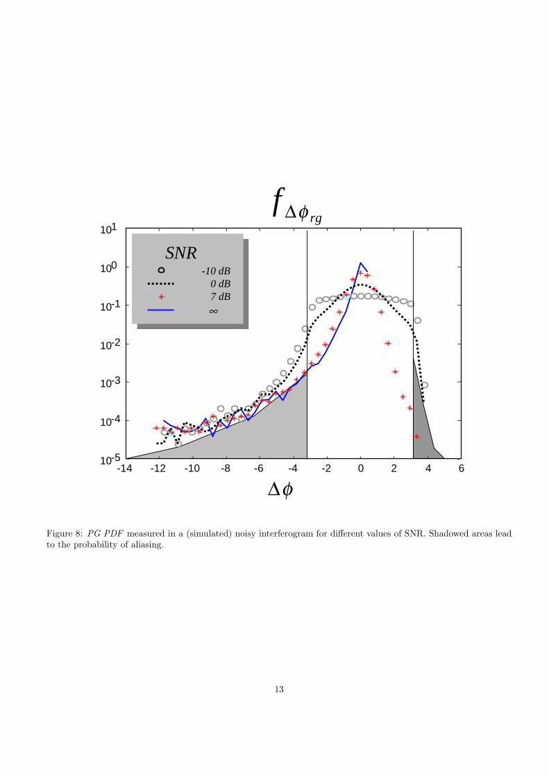
In the case or repeat pass interferometry we have to accounts for decorrelation sources, mostly due to temporalchanges. The effect of such noise on the phase of the interferogram has been studied under the assumption of aconstant slope[3]: we approximate the PDF there drawn as Normal PDF: N(o,σn), where σn is the variance of phasenoise and can be estimated from the coherence. The superposition of phase noise due to decorrelation and phasecontribution due to the topography results in the convolution of the two PDF. This convolution smears the peakof the PG-PDF in Fig. 7, hence increases the probability of aliasing, particularly in correspondence of the steepestgradients. As an example the PG PDF for different SNRs has been computed by adding noise to a set of simulatedInSAR acquisition, and is plotted in Fig. 8. Notice how the effect of noise is much more sensitive for the small andmedium PG values, depending also on the peakedness of the PDF, hence on the baseline. The PG-PDF derived insuch noisy environment, can be exploited to estimate the average number of residues, according to (14), and theninserted into the kernel of PU by providing the best estimate of the cost C in (13).

2.3 Interferogram flattening

Flattening is commonly implemented as a preliminary step to phase unwrapping (see for reference [1, 5, 3, 4]). Therationale of such approach lies in the statement that the most probable gradient in topography is zero. The aim offlattening is definitely to reduce the probability of aliasing, P (|∆φ−∆φf | > π) in (14). Unfortunately two misleadingassumptions make such approach not at all optimal: (1) it is not true that the most probable topographic gradientis zero (it is demonstrated in [8] for mountainous topographies); (2) the mapping between ground slopes and slopesin the SAR slant range reference is not linear, but rather strongly asymmetric. This mapping causes an asymmetryin the shape of the PG − PDF , and moreover shifts its center in the direction of the backslopes as appears fromFig. 7.

The optimal flattening, in the noisy environment just discussed, consists in finding the value ∆φf , that minimizesthe aliasing probability (14), the shaded areas in Figs. 7 and 8. This would require in turn the proper parametricmodel of the unwrapped PG-PDF, discussed in section 1.4. The marked asymmetry of the plots makes flatteningto be variant basing on the local topography, besides the baseline and noise, whose mean power can be retrieved bycoherence measures.

An example of the improvements that can be achieved by the optimal flattening is drawn in Fig. 9 that plotsthe probability of aliasing in the case of “conventional” flat earth compensation and for the optimal flattening hereproposed. Notice that the conventional approach may be optimal in some cases, however, the proper “flattening”can reduce the aliasing probability up to 50%.

2.4 Optimal azimuth averaging

Conventionally, interferograms are averaged in azimuth (complex multi-look), as azimuth resolution is finer thanrange. The main intent of averaging is to improve SNR, thus reducing the probability of PG aliasing. However, thereduction of azimuth sampling will proportionally scale the PG PDF, leading to a possible increase in the aliasingprobability. Clearly, an optimal azimuth “presumming” ratio is to be found, depending on the average topography,the acquisition geometry and the SNR. Here again, an optimization can be performed once that the azimuth PGPDF can be suitable modelled. The result of such optimization is plotted in Fig. 10 that shows the probability of PGaliasing as a function of azimuth presumming ratio: a SNR=0 dB was assumed and different baselines were tested(area of Naples). Notice that the proper presumming of a factor 2-5 is quite effective in reducing the PG PDF.

2.5 Average cut length and direction

Current PU techniques are designed to provide the minimal cut length or the minimal average cut height (L0, L1norm respectively). However, there are expected local cut lengths and directions, that depend on the topographyand the acquisition geometry. The knowledge of the cut statistics helps PU techniques. So far, the parametric model

12

-14 -12 -10 -8 -6 -4 -2 0 2 4 610-5

10-4

10-3

10-2

10-1

100

101rg

f φ∆

φ∆

SNR-10 dB

0 dB7 dB

∞

SNR-10 dB

0 dB7 dB

∞

Figure 8: PG PDF measured in a (simulated) noisy interferogram for different values of SNR. Shadowed areas leadto the probability of aliasing.

13

50 100 150 200 250 300 3500.01

0.02

0.03

0.04

0.05

Baseline [m]

�������������������

�������������������

� ���������������

� ���������������

PG: aliasing probability

SNR=0SNR=0

Figure 9: PG aliasing probability for the case of flat earth compensation and for the optimized flattening proposedin the paper.

14

1 3 5 7 90

0.005

0.01

0.015

0.02

0.025

# of range lines averaged

���������� Baseline:

100 m150 m200 m

Baseline:100 m150 m200 m

PG PDF

Figure 10: Azimuth PG aliasing probability for different presumming ratios and baselines. Simulated ERS interfer-ometry in the area of Naples.

for PG PDF is suited to compute the average number of cuts, here we will find a suitable approximation for theexpected cut length and direction.

Let ∆φ be the component of PG along a specific direction. The average cut length, Lm is the ratio between theprobability of aliasing: P (|∆φ| > π), and the spatial density λπ of π crossings:

Lm =E [P (∆φ > π)]

2λπ+E [P (∆φ < −π)]

2λπ

=E [P (|∆φ| > π)]

2λπ(15)

The computation of the density of π crossings is a rather complicated task in a general case. However for a Normal,zero mean process it is possible relate λπ to the second order statistics of the process [10]:

λπ =1π

√−r′′(0)r(0)

exp(− π2

2r(0)

)(16)

where the PG autocorrelation and its second order derivative in the origin, r(0) and r′′(0) can be computed byassuming the proper fractal power-law for the PG PSD. The average cut length that results by combining (15) and(16) can be estimated in different directions, hence providing information on the average cut direction.

As an example, Fig. 11 shows the cuts (values for which |∆φr| > π or |∆φa| > π) in a synthetic interferogram ofMt. Vesuvius (Bn=400 m).

The average cut length has been computed, for each direction, by applying (15) and (16) and compared withthat measured starting from the absolute PG values: the result is plotted in Fig. 12. The predicted value is alwayswithin the estimate one ±σL/2 (σL being the variance of the cut length): despite the approximations involved, themodel and the data crossings statistics fit well with the proper spectral estimate.

15

Figure 11: Wrapped synthetic phases simulating an ERS interferogram (Bn=400 m, 4 azimuth looks) achieved byexploiting the DEM of Mt. Vesuvius. The cuts, e.g. the values for which the range or the azimuth PG is in absolutevalue > π, have been marked in black.

16

0 10 20 30 40 50 60 70 80 900

1

2

3

4

5

6

7

Direction (deg)

Average cut length

Lm (

pixe

l)

Predicted Measured +σ/2Measured −σ/2

Figure 12: Average cut length predicted by the multi-fractal model as a function of the direction. The circles marksthe measures of the average cut length ± an interval equal to half its variance.

17

3 Acknowledgments

The author would thanks Dr. Alessandro Ferretti (Tele-Rilevamento Europa), who provided the introduction to PUtechniques and motivated the paper, and M. Ronchi who provided the computer simulations.

4 Conclusions

The modelling of earth topography by stochastic multi-fractal fields provides valuable information on the interfero-gram statistics. At a first instance, a parametric model for the PG PDF has been derived. Once that the parametersare retrieved by fitting the interferogram (the wrapped phase) PSD, the model is capable to predict the PDF ofthe unwrapped PG. This model has been exploited for simple and useful applications, like the determination of theoptimal interferogram flattening and the best azimuth presumming. Notice that the optimal flattening does notcorrespond to the compensation of flat earth, due to the highly asymmetric feature of the PG PDF. The use of anoptimal flattening can lead up to a 50% reduction is the number of singular points for some topographies / baselines.

Furthermore, the statistic of cuts, namely its mean length and direction has been derived and partly validated.The ultimate goal is an optimal phase unwrapping technique, not based on the minimization of any specific norm.

It should be based on a characterization of the reflectance model, dependent on topography statistics, and also onlocal reflectivity, vegetation, height, geological structure of rocks, and in general geomorphology.

18

References

[1] Andrew K Gabriel and Richard M Goldstein. Crossed orbit interferometry: theory and experimental resultsfrom SIR-B. Int.J. Remote Sensing, 9(5):857–872, 1988.

[2] Fuk K Li and R M Goldstein. Studies of multibaseline spaceborne interferometric synthetic aperture radars.IEEE Transactions on Geoscience and Remote Sensing, 28(1):88–97, January 1990.

[3] Richard Bamler and Philipp Hartl. Synthetic aperture radar interferometry. Inverse Problems, 14:R1–R54,1998.

[4] Paul Rosen, Scott Hensley, Ian R Joughin, Fuk K Li, Søren Madsen, Ernesto Rodrıguez, and Richard Goldstein.Synthetic aperture radar interferometry. Proceedings of the IEEE, 88(3):333–382, March 2000.

[5] Dennis C Ghiglia and Mark D Pritt. Two-dimensional phase unwrapping: theory, algorithms, and software.John Wiley & Sons, Inc, New York, 1998.

[6] C W Chen and H A Zebker. Phase unwrapping for large SAR interferograms: statistical segmentation andgeneralized network models. IEEE Transactions on Geoscience and Remote Sensing, 40(8):1709 –1719, August2002.

[7] F A Vening Meinesz. A remarkable feature of the earth’s topography, origin of continents and oceans. ProceedingsKoninklijke Nederlandse Akademie Van Wetenschappen Series B Physical Science, 54:220–229, 1951.

[8] Andrea Monti Guarnieri. SAR interferometry and statistical topography. IEEE Transactions on Image Pro-cessing, 40(12):2567–2581, December 2002.

[9] Umberto Spagnolini. 2–D phase unwrapping and instantaneous frequency estimation. IEEE Transactions onGeoscience and Remote Sensing, 33(3):579–589, May 1995.

[10] Athanasios Papoulis. Probability, Random variables, and stochastic processes. McGraw-Hill series in ElectricalEngineering. McGraw-Hill, New York, 1991.

[11] Andrea Monti Guarnieri, Paolo Biancardi, Davide D’Aria, and Fabio Rocca. Accurate and robust baselineestimation. In Second International Workshop on ERS SAR Interferometry, ‘FRINGE99’, Liege, Belgium,10–12 Nov 1999. ESA, 1999.

[12] D Schertzer and S Lovejoy. On the dimension of atmospheric motions. In Turbulence and Chaotic phenomenain fluids, chapter 5, page 505. Ed. T. Tatsumi, Elsevier North Holland, New York, 1984.

[13] W Feller. An introduction to probability theory and its applications. New York, 1971.

[14] Daniel Lavallee, Shaun Lovejoy, Daniel Schertzer, and Philippe Ladoy. Nonlinear variability of landscape topog-raphy: multifractal analysis and simulation. In L De Cola and N Lam, editors, Fractals in Geography, chapter 8,pages 158–192. Prentice Hall Englewood Cliffs NJ, 1993.

19

FIGURE CAPTIONS

Fig. 1. Above: simulated interferogram of Mt. Vesuvius, by assuming ERS-ENVISAT geometry. Below: (left)the DEM used for the simulation, (right) the DEM can be approximated locally as a complex sinusoid.

Tab. 1. Acronyms and parameters adopted in the paper.Fig. 2. Simplified InSAR geometry.Fig. 3. Comparison between the range PG PDF, measured on a synthetic (non wrapped) interferograms phase

(area of Naples) and its approximation, derived by transforming the range slope PDFFig. 4. Universal Multi Fractal Field (above), and the result after fractional integration (below). This stochastic

fractal provides a realistic DEM resemblance.Fig. 5. Residues due to noise and phase unwrapping. The pyramid in (a) has been converted into wrapped

phases, and then noise was superimposed. The resulting interferogram has then been filtered, giving the phases in(b). The residues have then been identified and marked as black / white pixels in (c) (depending on the sign). Thesole two residues due to topography are evidenced by arrows, all the other residues are due to noise and appear inclose pairs (one of these pairs has been marked by a white circle).

Fig. 6 (Left): the circles mark residues (or group of residues) measured on an interferogram simulated form thetrue DEM of Mt. Etna. (Right): the correct location of the ghost lines, as would appear on the unwrapped phase.The correct direction and length of ghost lines can be found only by accounting for topography statistics.

Fig. 7. Plots of the PG PDF measured on a synthetic fringe pattern of the Mt. Vesuvius (ERS InSARgeometry), compared with its parametric estimate derived by the (wrapped) interferogram, continuous line. The PGin the horizontal axis has been compensated for flat earth. The shaded areas measure the probability of aliasing.The PG values on the far left corresponds to layover.

Fig. 8. PG PDF measured in a (simulated) noisy interferogram for different values of SNR. Shadowed areas leadto the probability of aliasing.

Fig. 9. PG aliasing probability for the case of flat earth compensation and for the optimized flattening proposedin the paper.

Fig. 10. Azimuth PG aliasing probability for different presumming ratios and baselines. Simulated ERS inter-ferometry in the area of Naples.

Fig. 11 Wrapped synthetic phases simulating an ERS interferogram (Bn=400 m, 4 azimuth looks) achieved byexploiting the DEM of Mt. Vesuvius. The cuts, e.g. the values for which the range or the azimuth PG is in absolutevalue > π, have been marked in black.

Fig. 12. Average cut length predicted by the multi-fractal model as a function of the direction. The circles marksthe measures of the average cut length ± an interval equal to half its variance.

20