Uncertain Candidates, Voters with Valence, and the Dynamics of Candidate Position-Taking

Michael Bruter London School of Economics

Robert S. Erikson

Columbia University

Aaron Strauss Princeton University

March 19. 2007

Work on this paper is supported by an LSE-Columbia University Alliance grant. Prepared for the Conference on the Dynamics of Partisan Position Taking, Binghamton University, March 22-23, 2007.

Preliminary and Incomplete Draft

This paper introduces our project to model candidate positions where the following

conditions hold:

1. Candidates are uncertain about the median voter position

2. Candidates care about both winning and policy.

3. There exists candidate valence: One is more favored on non-policy grounds.

This set of assumptions can be recognized as a takeoff on Groseclose’s (2001) model of

candidate choice. The quest is for models of candidate equilibrium where the candidates

do not necessarily converge at the median voter position. .

Part 1 of this paper introduces the general problem of starting with the Downs

model but adding assumptions that are realistic, helpful, and tractable. Part 2 introduces

the Groseclose model. Part 3 discusses our variations in the model, a task that is largely

set in the future. Part 4 introduces some illustrations of equilibrium plots, found in the

eight figures at the end of this paper. Following Part 4 is a technical appendix further

describing our work.

1. Spatial Models of Two-Party Competition.

Elections are often modeled as a game between competing parties (or candidates) vying

for the allegiance of voters in ideological space. Typically the game involves two

candidates fighting over voters whose positions array on a single policy dimension.

However, voters can have non-policy motivations and candidates can care about policy as

well as election. And policy choices might involve more than one dimension

The standard starting point begin the discussion is the Downs (1957) model of

two-candidate competition. The two candidates are solely concerned about winning

elections. Voters are arrayed on a single left-right policy dimension and vote on the basis

1

of which candidate is closest to their views. The result, is that the candidates will

converge toward the center—toward the median voter. If each candidate is at the

median, the election is a tie. This result is also the Nash equilibrium, which means that if

either candidate departs from the median position, they lose the election.

Despite the unassailable Downsian logic that candidates gain (general election)

votes by moving to the center, the Downs model is obviously incomplete. Let us

describe the ways:

1. Voters vote on the basis of other things besides positions on a dominant policy (or

ideological) dimension. The result is that adopting the median voter position is no

necessary guarantee of electoral success.

2. Second, like voters, candidates are motivated (at least in part) by policy. Thus

they are motivated both by policy plus winning and holding office. Their

attraction to policy provides them with the incentive to risk diverging from the

median voter position.

3. Third, with voters caring about other things besides policy issues, it may be that

one candidate holds a net advantage apart from issues. This advantage could be

due to vestigial party loyalties or candidate charisma, or something else. The

theoretical literature describes this asymmetry of candidate popularity as a

“valence” advantage. A candidate’s valence advantage means that the median

position not only does not assure at least a tie. It also means that the median voter

position may not be the best position for a candidate.

4. Fourth, there may be uncertainty in the minds of the actors—so that voters might

not know candidate positions and candidates may be unsure of the electorates’

2

positions. Uncertainty by voters about candidates (e.g., Alvarez, 1997) will not

concern us here. But uncertainty by candidates about voters will.

5. Fifth, voters can be motivated by policy on more than one dimension, a situation

which according to theory can provoke all hell to break loose. With multiple

dimensions, Downs’s orderly median voter theorem breaks down in favor of

unruly indeterminacy and the specter of endless cycling.

All these considerations add complications and spice to the voting game.

Real-world candidates typically diverge from the median voter position And they

tend to be ideologically rigid, without the instability that non-equilibrium results might

seem to imply. Yet variations on the Downs model typically project the counterfactual

persistence of candidate convergence to the median or similar location. And they often

lead to at least the possibility of no candidate equilibrium.

Most post-Downsian theoretical treatments of the two-candidate game involve

trying to undo the likely lack of equilibrium in multiple dimensions or to convincingly

model candidate divergence. As discussed below, the present paper deals with both the

equilibrium problem and the convergence problem. The ideal is to present a model that

provides an equilibrium solution involving candidates who diverge ideologically rather

than the usual counterfactual prediction of convergence.

Probabilistic Voting

Under what conditions does the candidate game have an equilibrium? That is,

under what conditions is there a Nash equilibrium joint location in policy space from

which neither candidate has an incentive to depart? The alternative is no equilibrium—

no solution to the game and no particular prediction about candidate behavior. With

3

voters voting solely based on issues but with relevant issue preferences arrayed on more

than one dimension , the game generally lacks an equilibrium. Equilibrium in this case

can be restored via the realistic assumption that vote choice is a (sufficiently)

probabilistic rather than deterministic function of the voter’s position in ideological

space. The new equilibrium is a weighted mean of voter positions on the various issue

dimensions where voters are weighted by their perceived marginality, or the degree to

which candidates are uncertain of their vote choice (see, e.g., Erikson and Romero 1990).

Interestingly, while models of probabilistic voting increase the likelihood of

equilibrium in multidimensional models, they do so by taking away the preferred position

of one-dimensional models in terms of imposing order. Just as probabilistic voting

greatly expands the likelihood of an equilibrium in multiple dimensions if the voters’

error terms are sufficiently large, it also creates the likelihood of non-equilibrium in one-

dimensional models if the voters’ error terms are sufficiently small (but not zero). With

one dimension and candidate certainty about voter positions (and no valence imbalance),

the median voter position triumphs. With a small amount of candidate uncertainty about

individual positions, there is no equilibrium. With sufficiently large uncertainty about

individual positions, there is an equilibrium at the weighted mean.

Note that while the candidates know individual voter choices only with error, they

know the aggregation of the voters’ verdict. Thus, with probabilistic voting candidates

converge to a weighted mean that provides their best response to their opponent’s best

position. But if one candidate enjoys a “valence” ad vantage due to non-policy

considerations, they are the certain winner. Thus, unsatisfyingly, the losing candidate

moves to his best position in terms of vote share that happens to be their certain loss. It is

4

an irony that probabilistic models have too much certainty in that they imply that valence

rather than candidate behavior (at equilibrium) determines the winner.

Candidate Motivation, Uncertainty, and Convergence

Why in fact do not candidates converge as the simple Downs model predicts?

Instead of always competing for the median voter, the US Democratic and Republican

parties (and the UK Labor and Conservatives) are polarized with competing left and right

positions (of course to degrees that vary over time and geographical space) Subsequent

models to Downs have made important modifications. Some models allow candidates to

pursue policy and as well as electoral goals plus allow some uncertainty about the

outcome. But this by itself does not result in a prediction of divergent candidate

positions. Models that include candidate policy goals still leave the puzzle of why

candidates don’t move toward the center where they increase their chances of winning

rather than accepting a lottery between two competing ideological candidates.

One might expect a candidate with both policy and office-holding goals to edge

toward her preferred ideological position. However an important consideration is the

adverse policy consequence if an ideologically distasteful opponent is elected. The costs

of losing include not only losing office but also suffering under the opposition party’s

ideological regime.

As Calvert (1985) has shown, if there exists an equilibrium in the game with

uncertainty about the median voter position plus mixed motives by the candidates, it

remains in the close vicinity of the median voter position. And once uncertainty about

the median voter location is introduced, even in one dimension there is no guarantee of

5

the existence of an equilibrium location. Thus, the added realism of candidate

uncertainty plus policy motivated candidates leaves us unsatisfied..

Valence

In the Calvert-type model, no bias exists, so that at equilibrium each candidate has

an equal chance of election. The convenience of this assumption is that maximizing the

expected vote margin is identical to maximizing the chance of victory. Suppose we

introduce the complication of bias in the form of a valence advantage to one candidate.

Now, maximizing victory is different from maximizing the expected vote. The payoff is

a set of interesting results.

“Valence” refers to the candidate advantage where one candidate is more popular

than the other, Without valence (bias), when the candidates are similar in their policy

positions or at some other joint equilibrium, the expected outcome is a tie. With non-zero

valence (one candidate favored), uncertainty about the location of the median voter, plus

candidates who care only about winning, there is an absence of equilibrium even in one

dimension.

The intuition is simple. The underdog knows with certainty that he will lose if he

copies the advantaged candidate. Consequently the underdog seeks a more extreme

position in order to create an ideological opening between him and the advantaged

candidate. This allows the possibility, perhaps slim, that the underdog is close enough to

the uncertainly located median voter to offset the leading candidate’s valence advantage.

Meanwhile, no matter where the underdog goes in one-dimensional ideological space, the

leader will chase him and copy his position so that with the same ideological positions,

the leader’s valance advantage ensures the leader’s victory. The net result is an endless

6

game with one candidate forever chasing the other. There exists an analogy to yacht

racing. As the race’s end approaches, the leader does not want to see the lagger take a

different and possibly more successful course to the finish line. If they are on the same

course, the leader will stay ahead. (For a general discussion of pursuit theory, see Nihan,

2007 forthcoming). In this game with an uncertain median voter location and valence

asymmetry plus election-seeking candidates, the only equilibrium that can be achieved is

from the unsatisfying artifice of a mixed strategy (Aragones and Palfrey, 2002).1

Suppose, however, we add a dose of policy-seeking on the part of the candidates

so that they want to win but also care about policy. Now our model includes candidates

who are both office-seeking and policy-seeking, asymmetrical candidate valence, and

candidate uncertainty about the location of the decisive median voter.

A key here is the presence of a decisive median voter who is decisive even though

individual voters’ decisions presumably are known only probabilistically. This can be

accomplished at the sacrifice of assuming a one-dimensional model where the voters to

the left of the median voter appear as the symmetrical opposite of the voters on the

median voter’s right. In this instance, the decisive median voter is also the (weighted)

mean voter as well.2

2. The Groseclose Model

In an important article, Groseclose (2001) has elaborated on the properties of the

candidate game with non-zero valence (one candidate favored), uncertainty about the

1 See also Ansolahebere and Snyder, 2000. 2 Since we are concerned with the valence as it affects the median voter, the source of the valence advantage need not simply be perceptions of candidate competence or charisma, as is usually presented. The valence could be simply party identification, as when one candidate has an advantage due to the district being favorable to the candidate’s party in terms of long-standing partisanship.

7

location of the median voter, and candidates who care about both policy and winning, the

following is now known. The highlights are:

1. If there exist an equilibrium, the disadvantaged candidate will move away from

the center toward his preferred position, while the advantaged candidate will

move toward the center from her preferred position.

2. There may not be an equilibrium. Even in one dimension, the game may not have

a solution (except possibly involving the artifice of allowing mixed strategies—as

if candidates roll dice simultaneously). As the uncertainty about the median voter

declines toward zero, the game reverts to the Aragones and Palfrey game where

the leader chases the underdog,

By the first point, less attractive candidates may have little hope of winning, but their

only hope may be that the median voter, whose position is uncertain, may by some slim

chance share their position. In effect the loser throws a “hail Mary,” which under some

conditions is expected to lose votes but does maximize the slim chance of victory. If,

contrarily, the disadvantaged candidate mimics the position of the dominant candidate,

the disadvantaged candidate will lose with greater certainty.

The second point is that as uncertainty shrinks the equilibrium is lost. This

absence of an equilibrium means that no matter how one candidate responds (in terms of

ideological positioning) to the opponent’s positioning, the opponent can improve his or

her electoral outlook by moving. This would be followed by the first candidate re-

positioning, etc. In short, there could be no set of dominant candidate and dominated

candidate positions whereby neither candidate has an incentive to move.

8

Groseclose’s model assumes voters and candidates’ issue loss functions are

concave, and more specifically the usual quadratic loss function. He draws his rich set

of conclusions with a stylized model where the candidates’ preferred policy positions are

equidistant from the median voter and where except for contrasting policy preferences,

the candidates’ objective functions and perceptions of the median voter are identical.

Although seemingly restrictive, these assumptions are useful simplifications for obtaining

comparative statics.3

3. The Bruter-Erikson-Strauss Agenda

The intent of our project is to generalize Groseclose’s result. At this juncture, we

have prepared various illustrations of equilibrium (or its absence) under various

conditions. The appendix to this paper contains the derivation of our model along with

our methodology for searching for equilibria in our examples. We plan to derive further

analytical results beyond Groseclose’s version of the model in several ways. Following

Groseclose, we plan to vary the error variance of candidate perceptions and vary the

candidates’ relative preferences for office-holding versus policy. We use Groseclose’s

starting point whereby the candidates weight the two goals identically and believe the

identical error variance. In other words we start by making the same varying adjustments

for each candidate.

We plan to eventually try variations where we eliminate symmetries—for instance,

modifying candidate policy preferences so they are different distances from the median

voter. Sometimes the valence-favored candidate is closer to the median voter and

sometimes farther. We also plan to vary the candidates’ relative preference for policy

3 For extensions to multiple parties and dimensions, see Schofield, 2004,

9

versus governing when a favorite and when the underdog.. And we plan to vary the

variance of the error with which they see the median voter position and allow candidates

to view the median voter with varying expectations rather than a common perceptions.

Adding uncertainty about valence

We also intend to explore models where the uncertainty is over the valance rather

than over the median voter position. This alternative model could yield different

predictions. One intuition is that a quite different result would obtain, that the underdog

would move toward the center and the favorite would move away toward her ideal point.

For a final level of realism, we intend to model contests where uncertainty exists about

both candidate valence and the median voter position.

Modeling electorates rather than the median voter

A further enrichment would be to relax the assumption that the median voter is

pivotal. (The median voter is pivotal if the electorate is distributed symmetrically on one

ideological dimension or in multiple dimensions with radial symmetry). Here we would

model not only the probable vote of one pivotal median voter but rather integrate over a

density of voters at various policy positions with individual variation in valence.

Modeling the vote response of an electorate instead of a median voter would also allow

the search for possible equilibrium properties when issue-space is multidimensional and

or there exist peculiar asymmetrical densities of voters in issue space..

4. Illustrations

Our simulations are performed computationally over grids involving policy

choices of two candidates, the Democrat with a preferred policy position to the left of the

median voter and the Republican whose preferred policy position is to the median voter’s

10

right. The simulations will work as follows. For each set of assumptions, we first set the

Democrat’s platform at a discrete set of positions, separated by small regular intervals.

For each possible platform position, we determine the Republican candidate’s best

response. Then we repeat the procedure, estimating the Democrat’s best responses to the

Republican’s possible positions. When the two sets of best responses are graphed against

each other (on separate axes), where the lines cross is the equilibrium point. When the

lines fail to cross, there is no equilibrium. See also the technical appendix.

For most of the illustrations that follow, the Democrat’s preferred position is at - 1

while the Republican’s is at +1. The median voter’s position always has an expectation of

zero. Our starting point regarding the variance of the median voter position is that the

variance is .01 (a standard deviation of .10). This assumption is imposed in order to make

the model plausible. Given today’s plethora of polls, one might argue with some

conviction that candidates can learn the median voter’s location has little error variance.

But if the variance were zero, candidates would be observed to converge as a dominant

strategy. . Relative to the gap between the preferred positions of ideologically polarized

Republican and Democratic candidates, the variance of the candidate’s uncertainty about

the median voter position is greater than epsilon.

Following is commentary on eight illustrative equilibrium plots, In the annotation,

please note an inconsistency in our notation. In the model in the appendix, we set the

weight for policy to 1.0 and vary the weight for winning office. In our annotations, we

assume the weight for winning is 1.0 and vary the weight for policy. This of course

presents no loss of generality.

11

Figure 1. A close race. No valence advantage. Candidates care about policy (mostly).

Perfectly symmetrical, small deviation from median voter for both candidates. Outcome

is a coin flop.

Figure 2. A Democratic advantage. The Democrat has a decent valence advantage and

has a large probability of winning (95%). Moving closer to the center does not help the

Republican as they don’t gain much chance of winning and lose “policy” utility. As

predicted by Groseclose, the valence advantaged candidate is closer to the median voter.

Figure 3. No equilibrium. The Democrat again has a valence advantage, but this time

the candidates only care about winning.; note the discontinuity at 0 of the Republican

candidate’s best response. The Democrat simply wants to “shadow the Republican”.

Figure 4. Large Democratic Advantage. Similar to the case where the Democrat had

the smaller valence advantage, the Democrat is almost assured victory. The candidates

have now diverged farther from the median, as the Democrat is able to move closer to

his/her ideal point.

Figure 5. High Uncertainty. Similar to the “close race” plot, but now the candidates

have diverged further away from the median, as they are uncertain where the median

actually is. They diverge only because they care about policy.

Figure 6. A mixed bag. Idealistic Democratic incumbent against moderate GOP

challenger. The Democrat enjoys a slight valence advantage, and lower uncertainty of

median voter. The Democrat is a liberal idealist with an extreme ideal point (-1) and cares

mostly about policy. The challenger is moderate (+0.1 ideal point) who cares mostly

about winning. The Democrat’s chance of survival: 62%.

12

Figure 7. _Moderate Republican Favored. A moderate Republican with a valence

advantage is more certain about median voter than the opponent, and cares about winning

more than the opponent. Note that the Republican heads right for the median voter voter

and has a large chance of success: 84%

Figure 8. Introducing Valence Uncertainty. This is a symmetric election, but this

time with uncertainty about valence and no uncertainty about the median voter position..

Again, we find divergence.

Appendix In this technical appendix, we first describe the candidate model, which is a general

version of the Groseclose model given quadratic loss as the functional form of candidate

and voters’ issue loss. Candidates care about policy and winning. The median voter

cares about policy but also has a valence (relative attractiveness) toward the candidates

apart from policy.

Second, we describe how we transport the model to graph the equilibrium location under

varying scenarios.

Legend: U=Utility of the Democratic Candidate B=bliss point (ideal point) of the Democratic candidate X=the Democratic candidate’s public policy position, the object of our attention R=the Republican candidate’s public policy position 0=zero=expectation of the median voter position P=probability of a Democratic victory 1=one=Democratic Candidate’s Policy Weight W=value of winning to Dem. Candidate (relative to Policy weight) u=error in estimate of the median voter position s=standard deviation of the median voter position (M) M=0+u = median voter position where standard deviation of u=s a=valence or intercept term for the median voter, the median voters’ relative liking for the Democrat over the Republican..

13

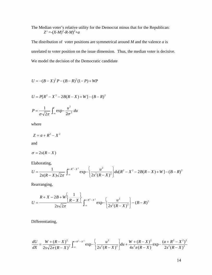
The Median voter’s relative utility for the Democrat minus that for the Republican: Z’ =-(X-M)2-R-M)2+a The distribution of voter positions are symmetrical around M and the valence a is

unrelated to voter position on the issue dimension. Thus, the median voter is decisive.

We model the decision of the Democratic candidate

WPPRBPXBU +−−−−−= )1()()( 22

222 )(])(2[ RBWXRBXRPU −−+−−−=

∫ ∞−−=

Z uP 2

2

2exp

21

σπσdu

where

22 XRaZ −+=

and

)(2 XRs −=σ Elaborating,

22222

2

)(])(2[)(2

exp2)(2

1 22

RBWXRBXRduXRs

uXRs

UXRa

−−+−−−⎭⎬⎫

⎩⎨⎧

−−

−= ∫

−+

∞−π Rearranging,

222

2

)()(2

exp22

1222

RBXRs

us

XRWBXR

UXRa

−−⎭⎬⎫

⎩⎨⎧

−−⎭

⎬⎫

⎩⎨⎧

−+−+

= ∫−+

∞−π

Differentiating,

22

222

2

2

22

2

2

2

)(2)(exp

)(4)(

)(2exp

)(22)( 22

XRsXRa

XRsXRWdu

XRsu

XRsXRW

dXdU XRa

−−+

−−−+

+⎭⎬⎫

⎩⎨⎧

−−

−−+

= ∫−+

∞− ππ

14

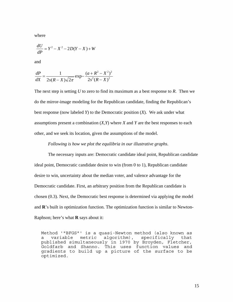
where

WXYDXY

dPdU

+−−−= )(222

and

22

222

)(2)(exp

2)(21

XRsXRa

XRsdXdP

−−+

−−

=π

The next step is setting U to zero to find its maximum as a best response to R. Then we

do the mirror-image modeling for the Republican candidate, finding the Republican’s

best response (now labeled Y) to the Democratic position (X). We ask under what

assumptions present a combination (X,Y) where X and Y are the best responses to each

other, and we seek its location, given the assumptions of the model.

Following is how we plot the equilibria in our illustrative graphs.

The necessary inputs are: Democratic candidate ideal point, Republican candidate

ideal point, Democratic candidate desire to win (from 0 to 1), Republican candidate

desire to win, uncertainty about the median voter, and valence advantage for the

Democratic candidate. First, an arbitrary position from the Republican candidate is

chosen (0.3). Next, the Democratic best response is determined via applying the model

and R’s built in optimization function. The optimization function is similar to Newton-

Raphson; here’s what R says about it:

Method '"BFGS"' is a quasi-Newton method (also known as a variable metric algorithm), specifically that published simultaneously in 1970 by Broyden, Fletcher, Goldfarb and Shanno. This uses function values and gradients to build up a picture of the surface to be optimized.

15

This “best response” position is assigned to the Democratic candidate. The “best

response” for the Republican candidate (given this Democratic position) is then

determined in the analogous way. This iterative process is repeated 100 times or until

both candidate positions do not change by more than 10^-4. If this convergence condition

is not met after 100 iterations, we assume there is no equilibrium.

For the plots themselves, the “best response” procedure is applied to both

candidates, letting their opponent’s position vary from -2 to 2 at intervals of 0.05. The

Democrat’s best response at each of the Republican’s positions is plotted with a blue

dashed line connecting each of these best response points. The Republican’s best

response is plotted using a solid red line.

In the lower right, the equilibrium positions of the Democratic and Republican

candidates are reported (if an equilibrium exists). The Democratic probability of winning

at equilibrium (the Democrat’s uncertainty—if it differs from the Republican’s—taken as

given) is also reported.

16

References

Alvarez, Michael. 1997. Information and Elections. Ann Arbor: University of Michigan Press. Ansolahebere, Stephen D.and James M. Snyder, Jr. 2000. “Valence Politics and Equilibrium in Spatial Election Models.” Public Choice. `03: 327-336. Aragones, Enriqueta and Thomas R. Palfrey. 2002. “Mixed Equilibrium in a Downsian Model with a Favored Candidate.” Journal of Economic Theory 103: 131-161. Calvert, Randall L. 1985. “Robustness of the Multidimensional Voting Model: Candidate Motivations, Uncertainty, and Convergence. American Journal of Political Science 29:69-95. Downs, Anthony. 1957. An Economic Theory of Democracy. New York: Harper & Row Erikson, Robert S. and David W. Romero. 1990. “Candidate Equilibrium and the Behavioral Model of the Vote.” American Political Science Review 84 (December): 1103-1125. Groseclose, Tim. 2001. “A Model of Candidate Location When One Candidate Has a Valence Advantage.”American Journal of Political Science.” 45 (October): 862-886. Nabin, Paul J. 2007, forthcoming. Chases and Escapes: The Mathematics of Pursuit and Evasion Princeton: Princeton University Press. Schofield, Norman. 2004. “Equilibrium in the Spatial Valence Model of Politics.” Journal of Theoreetical Politics. 16: 447-481. .

17

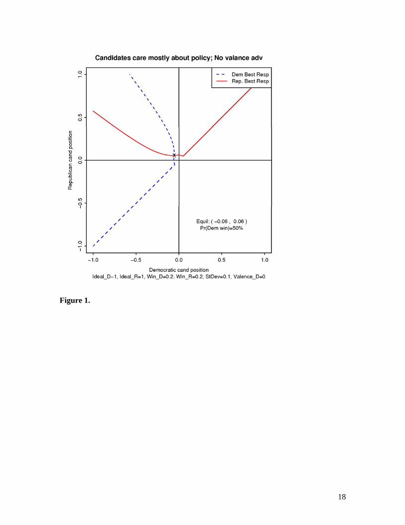
Figure 1.

18

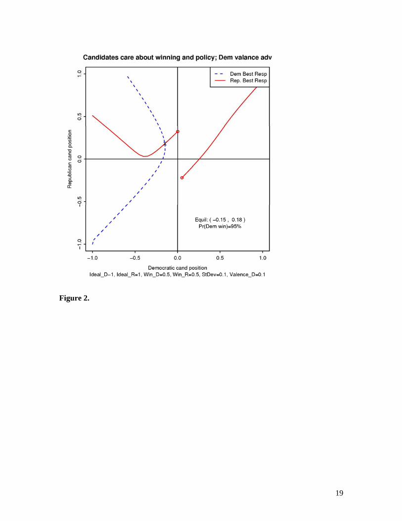
Figure 2.

19

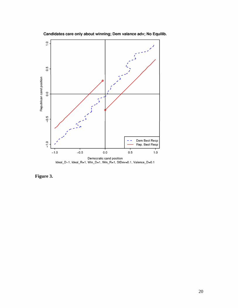
Figure 3.

20

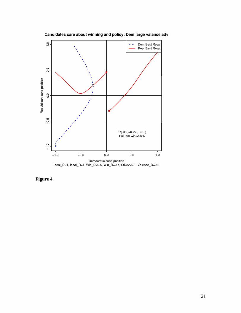
Figure 4.

21

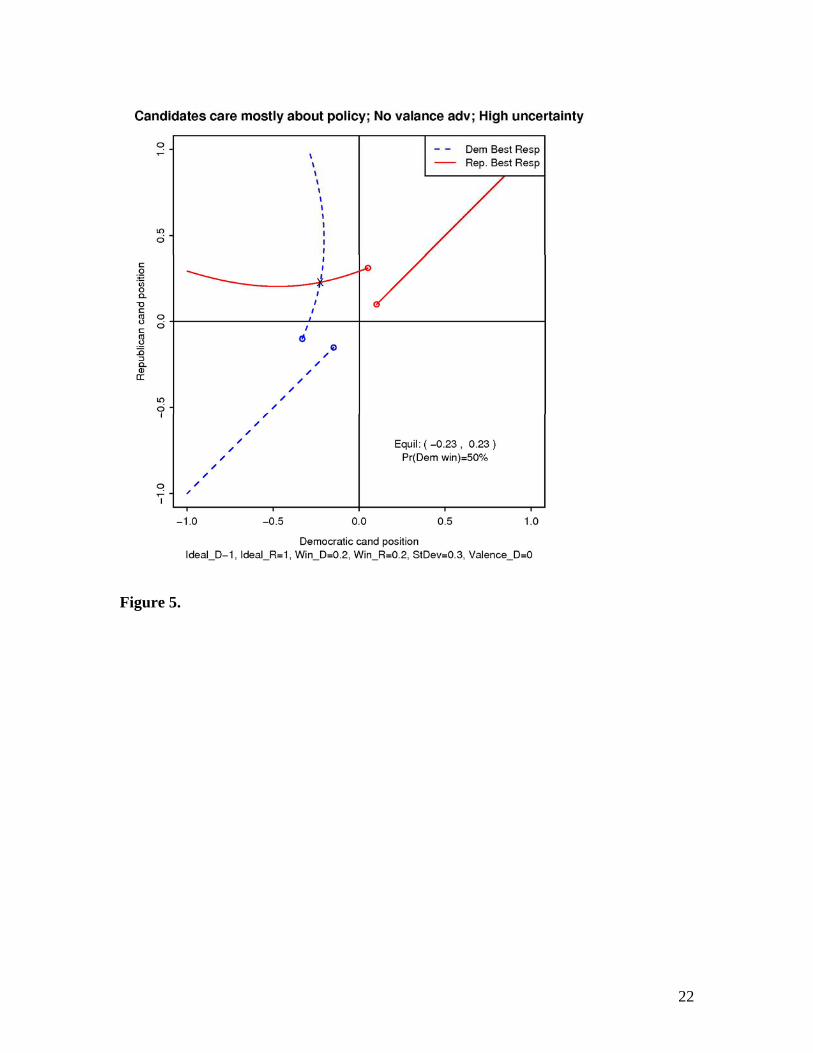
Figure 5.

22

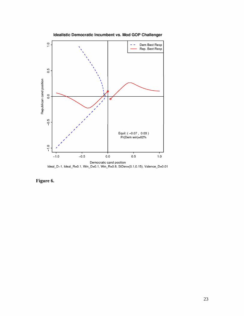
Figure 6.

23

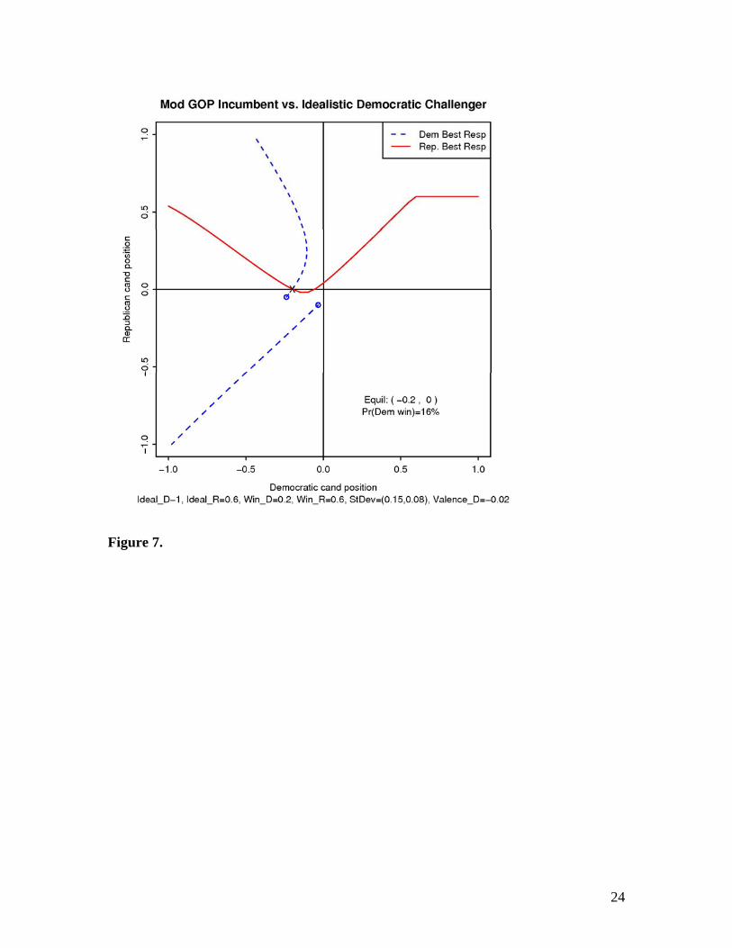
Figure 7.

24

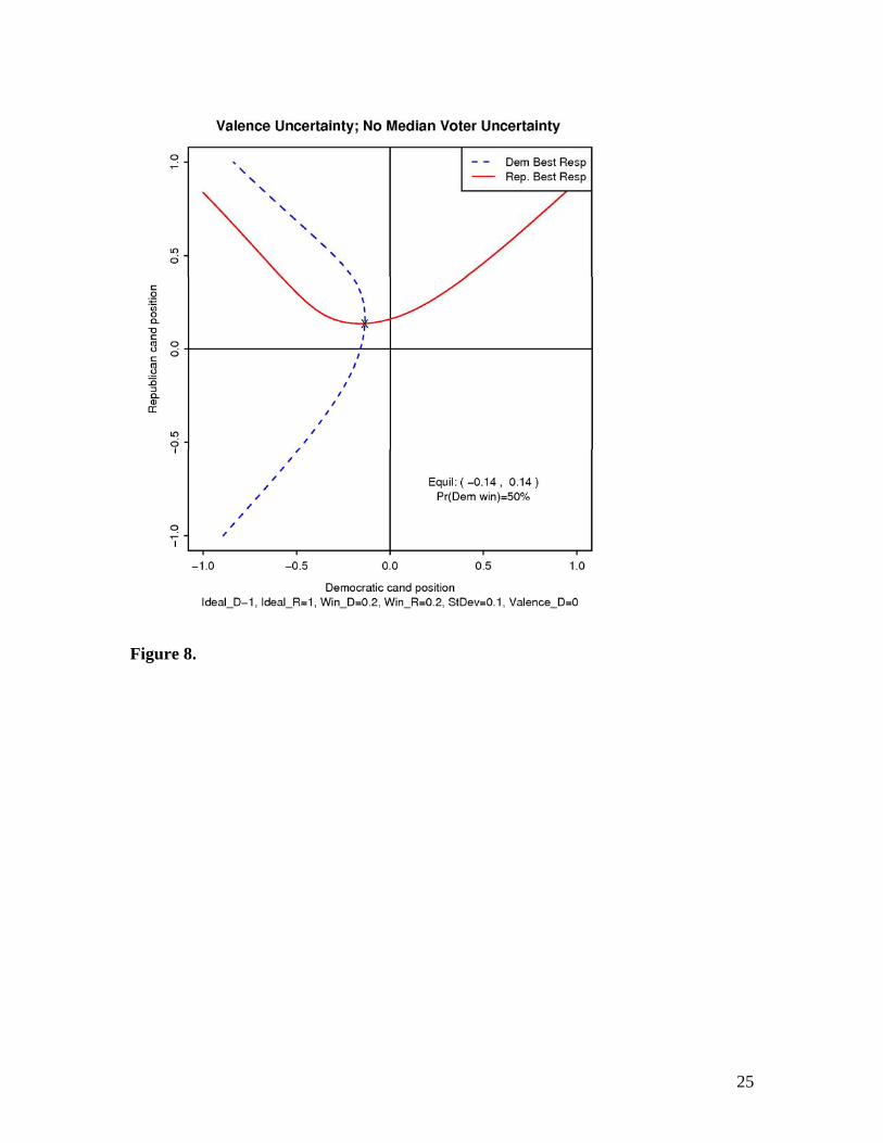
Figure 8.

25