the twelve lectures in the (non)commutative geometry …preprints.ihes.fr/2012/m/m-12-13.pdf · the...

The twelve lectures in the (non)commutative geometryof differential equations

Arthemy KISELEV

Institut des Hautes Etudes Scientifiques

35, route de Chartres

91440 – Bures-sur-Yvette (France)

Juillet 2012

IHES/M/12/13

THE TWELVE LECTURES

IN THE (NON)COMMUTATIVE GEOMETRY OF

DIFFERENTIAL EQUATIONS

ARTHEMY V. KISELEV

Abstract. These notes follow the twelve-lecture course in the geom-etry of nonlinear partial differential equations of mathematical physics.Briefly yet systematically, we outline the geometric and algebraic struc-tures associated with such equations and study the properties of thesestructures and their inter-relations. The lectures cover the standard ma-terial about the infinite jet bundles, systems of differential equations(e.g., Lagrangian or Hamiltonian), their symmetries and conservationlaws (together with the First and Second Noether Theorems), and theconstruction of the nonlocalities. Besides, in the lectures we introducethe calculus of variational multivectors — in terms of the Schouten bra-cket, or the antibracket — on the (non)commutative jet spaces and pro-ceed with its applications to the variational Poisson formalism and theBRST- or BV-approach to the gauge systems.

The course differs from other texts on the subject by its greater em-phasis on the physics that motivates the model geometries. Simultane-ously, the course attests to the applicability of the algebraic techniquesin the analysis of the geometry of fundamental interactions. These lec-tures could be a precursor to the study of the (quantum) field and stringtheory.

Date: July 2, 2012.2010 Mathematics Subject Classification. 37K05, 37K10, 53D55, 81T13, 81T75; also 17B80, 35Q53,

35Q61, 37K30, 37K35, 53D17, 58D15, 81T30, 81T70; general 51P05, 53Z05, 58E30.Key words and phrases. Jet bundles, symmetries, conservation laws, Noether theorems, gauge sys-

tems, Poisson structures, deformation quantisation, noncommutativity, Lie algebroids, BRST- andBV-differential.

Address : Johann Bernoulli Institute for Mathematics and Computer Science, University of Gronin-gen, P.O. Box 407, 9700 AK Groningen, The Netherlands. E-mail : [email protected].

1

2 ARTHEMY KISELEV

Contents

Foreword 4

Introduction 5

Part I. Lagrangian theory 8

1. Jet space and structures on it 91.1. Vector fields on J∞(π) 131.2. Differential forms on J∞(π) 15

2. Differential equations E∞ ⊆ J∞(π) 20

3. Symmetries of differential equations 273.1. Classical symmetries of the Burgers equation 333.2. Symmetry-invariant solutions of the Liouville equation 37

4. Conservation laws 404.1. Generating sections of conservation laws 424.2. The homotopy formula 46

5. Euler–Lagrange equations 545.1. First Noether Theorem 56

6. Gauge symmetries 606.1. Maxwell’s equation 62

7. Nonlocalities 677.1. Nonlocal symmetries 707.2. Recursion differential operators 727.3. Nonlocal recursion operators 73

Part II. Hamiltonian theory 77

8. The calculus of noncommutative multivectors 788.1. Noncommutative multivectors 828.2. Noncommutative Schouten bracket 83

9. Noncommutative Poisson formalism 879.1. Poisson brackets 879.2. Completely integrable systems 899.3. Deformation quantisation 91

10. Lie algebroids over jet spaces 9710.1. Classical Lie algebroids 9710.2. Variational Lie algebroids 10110.3. Homological evolutionary vector fields 108

THE TWELVE LECTURES 3

11. BRST- and BV-formalism 114

12. Deformations of nonlocal structures 12012.1. Backlund (auto)transformations 12012.2. Gardner’s deformations 12412.3. Zero-curvature representations 127

References 134

4 ARTHEMY KISELEV

Foreword

Every block of stone has a statue inside it andit is the task of the sculptor to discover it.

Michelangelo

This course is aimed to teach. Any other goals, such as: to bring more rigour into thetreatment, to make the calculus more axiomatic, to reveal the possibilities of a furthergeneralization, to reformulate the setup in coordinate-free algebraic terms, to broadenthe horizons, and to bridge the gaps — or similar pontific activities — are secondary.

These notes do not contain any previously unknown, unpublished facts. The authorrather faced the task of selection and systematization of the set of basic definitions,properties, and algorithms. The course communicates the bare minimum of the geo-metric theory in the amount which is practically useful for a mathematical physicist.The lectures indicate the applicability and limitations of this theory. Simultaneously,they prepare the curious scholar to a deeper study of the subject: the book [100], whichhas become the standard reference, and the book [79], which describes the applicationof the advanced algebraic techniques to differential equations, are highly recommendedas the follow-up reading. The lectures also facilitate the understanding of the contextand results in the current journal publications on this subject.

These notes are based on the lectures which were read by the author in the springsemesters in 2009 (at Utrecht University) and 2012 (at the University of Groningen).In the present form, the twelve chapters schedule the full-week course, lasting for sixdays with two standard lectures and one exercise class on each; on the seventh day, theaudience experiences the shift of the paradigm.

The author declares his sole responsibility for the selection (resp., omission) of the ma-terial and its presentation. The arrangement of the topics reflects the author’s personalview how the geometry of differential equations could be taught to the prepared novices.Each example or illustration, whenever quoted here for the educational purposes, is tobe acknowledged as a token of gratitude to its author(s). Any discrepancies, instancesof the incompleteness, factual errors (if any), or any mismatches in the notation areunintentional and should be promptly reported to the author.

Acknowledgements. A part of the research which contributed to this text was performedby the author at the IHES (Bures-sur-Yvette); the financial support and hospitality ofthis institution are gratefully acknowledged. The author’s research was also support-ed in part by NWO VENI grant 639.031.623 (Utrecht) and JBI RUG project 103511(Groningen1 ). The author is grateful to M. Kontsevich and to B. A. Dubrovin andYu. I. Manin for illuminating discussions and also thanks J. Krasil’shchik, J. W. vande Leur, P. J. Olver, and A. Verbovetsky for discussions, stimulating remarks, andconstructive criticisms.

1The author thanks R. van Breukelen, J. Dooper, P. Helminck, M. Hoekstra, G. Senden, andM. Soeten for TEXnical assistance and also S. Ringers who read and commented on the first draft ofthis manuscript.


Introduction

These lectures in the geometry of nonlinear partial differential equations are devised forthe students of mathematical and physical specializations who learn this discipline forthe first time. The course acquaints the audience with the main notions and concepts;it neither fully covers the vast set of geometries nor reports all the modern methodsand techniques. However, we believe that the familiarity with the language of jetbundles, which are ambient to differential equations, is indispensable to the specialistsin classical mathematical physics (such as the General Relativity) and its quantisation(e. g., QED, QCD, or string theory[38, 102]). It must be noted that the techniques andstatements from the traditional paradigm of smooth manifolds, be they Poisson or bethey the configuration spaces of the Euler–Lagrange systems, may no longer fully graspthe geometries of those models from QED, QCD, etc.

The course unveils the relations between the models of physical phenomena and thegeometry behind such models. It outlines the limits of the applicability of the models.It then becomes possible to focus on the sets of initial axioms and sort out the adhoc assumptions from the conceptual hypotheses such as the gauge invariance or thepresence of infinitely many integrals of motion.

The course communicates the following skills:

• finding particular (classes of) solutions of nonlinear partial differential equations,and propagation of the already known solutions to families;• finding the integrals of motion (more generally, finding the conserved currents);• finding the variational Poisson structures and verification that a given (non)com-

mutative bi-vector is Poisson;• by using the same calculus of variational multivectors and involving the struc-

tures which are pertinent to the gauge systems, the introduction of the BRST-and BV-differentials and the construction of the extended BV-action that sat-isfies the classical variational master equation;• inspecting whether the “spectral” parameter in a given zero-curvature represen-

tation is or is not removable by the gauge transformations.

In the narration, we balance between the coordinate-independent reasonings andthe operation in local coordinates. To motivate and illustrate the main notions andconstructions, we restrict ourself to the reasonable set of model equations. Never-theless, these examples are multi-faceted so that they fit for all purposes. Such arethe kinematic-integrable, bi-Hamiltonian Korteweg–de Vries equation (i. e., the Drin-feld–Sokolov equation[22] associated with the root system A1), the Darboux-integrableLiouville equation (i. e., the nonperiodic 2D Toda chain associated with the root sys-tem A1), and the Maxwell equation (i. e., the Yang–Mills equation with the abeliangauge group U(1)).

At the same time, we balance between the maximal generality and the concreterealization of the abstract structures: for instance, we consider the homological equationQ2 = 0 on the jet super-spaces and from it we derive the (non)commutative variationalPoisson formalism and the BRST- and BV-techniques.

6 ARTHEMY KISELEV

The examples often indicate the branching point of theories and mark the exits fromthe main road to other concepts,[12] geometries,[23] and methods such as the supersym-metry, inverse scattering,[27] Hirota’s tau-function,[96] (Poisson) vertex algebras,[46] theYang–Baxter associativity equation,[104] or homotopy Lie structures[84] — to name onlya few.

The superposition of mathematics and physics in this text makes it different fron ei-ther a traditional treatise on the formal geometry of differential equations or the reviewson gauge fields or Poisson mechanics. For a working mathematician, our approach mayseem not entirely axiomatic. A theoretical physicist who waits to apply the new calculusin the own models will first face the great multitude of preliminary concepts which aredeclared to be the pre-requisites. We also note that we by-pass the detailed considera-tion of the finite jet spaces;[105] instead, we spend an extra time on the nonlocalities overthe infinite jet spaces. Likewise, we study the “generic,” higher-order Hamiltonian op-erators and thus, again, pass over the geometry of the hydrodynamic-type evolutionarysystems.[24]

Summarizing, in these lectures we substantiate the key facts and mark the links toother domains of science.

Let us make several technical but important assumptions about the class of geometrieswhich we are going to consider. The ground field will always be R and the real dimensionn ∈ N of the base manifold Mn in the fibre bundles can be arbitrary positive integer(unlike n = 1 in CFT or in many surveys on the KdV-type systems). We study the non-graded setup of purely even manifolds and bundles. The odd neighbours will appearin due course: the parity reversion Π will be performed by hands, which will be statedexplicitly. We do not develop on the plurality of the quantisation techniques (e. g., thedeformation- or the BRST/BV-quantisation) which become available as soon as the jetbundle formalism is elaborated. Nor do we track the relation between the geometryof jets and the quantum groups, quantum integrable systems, and the classical Yang–Baxter equation. Although we introduce the calculus of variational multivectors in thenoncommutative setup ab initio, the analysis stays at the non-quantum level (i. e., thePlanck constant ~ almost never appears, with two important exceptions).

Unless it is stated otherwise, all maps (including those which define the smoothnessclasses of manifolds) are assumed to be infinitely smooth yet possibly not analytic.We emphasize that the power series “solutions” of the formally integrable differentialequations can diverge outside the central point. This subtlety projects (1) onto ourchoice of the classes of sections of the bundles (so that we shall sometimes assume, forthe vector bundles, that either the supports are finite, or the sections rapidly decay atthe infinity, or are periodic but the period is not known in advance), and also projects(2) onto our hypotheses about the topology of the base manifolds (always assumedoriented) and of the total spaces of the bundles. Namely, the local triviality assumptioncan become insufficient whenever one attempts to integrate by parts or calculate thevalue of a functional at a given section by taking the integral over the entire base. Thus,the choice of the section classes versus the compactness of the base is correlated withthe analytic integrability of the functionals. Usually, we shall discard the aspects of


topology. Likewise, we consider the spaces of jets of sections for the (vector) bundlesbut not the jets of submanifolds.

Lie groups and algebras are of course present, but their role is not emphatic (c. f. [22,104]). On the same grounds, we exploit the geometric roots of the (non)commutativePoisson structures but avoid their study via the Fourier transform that converts theminto the W -algebras and a suitable analog of the quantum BRST.[13]

The geometry of spaces of infinite jets for sections of vector bundles admits theimmediate generalizations to the Z2-graded setup of supermanifolds,[77] to the jetspaces for maps of manifolds, and to noncommutative geometry. The calculus of(non)commutative variational multivectors has its renowned applications in the Hamil-tonian formalism and in the geometry of the Euler–Lagrange gauge-invariant systems;both concepts are intimately related to the quantum string theory. The formalism alsoserves the following three model descriptions of the scattering: the Kontsevich defor-mation quantisation[68] (governed by the associativity equation[118] |1〉 ⋆ (|2〉 ⋆ |3〉) =(|1〉 ⋆ |2〉) ⋆ |3〉 for the in-coming states |i〉), the pairwise-interaction factorization inHirota’s tau-function, and the inverse spectral transform. The correlation between thejet bundle formalism and Feynman’s path integral approach to the quantum world isyet to be explored: there is more about it than meets the eye.

8 ARTHEMY KISELEV

Part I. Lagrangian theory

While studying classical mechanics,[2, 85] we considered[51] the static, kinematics, anddynamics of material points: respectively, we analysed the structure of the configurationspaces, the non-relativistic motion along the true trajectories, and the interaction ofmassive particles in space (or in any suitable curved manifold). Special relativity theoryallows us to approach the speed of light in the description of the motion of such points.Yet in both cases the objects were not stretched in space (e. g., they were like theelectron — alternatively, the finite size of the objects could be neglected, such as inKepler’s problem problem for the attracting spheres). Besides, the objects did notcontain any internal, hidden degrees of freedom which would determine the hypotheticfifth and, possiblly, higher dimensions that stay invisible for us.

However, the high-energy scattering experimentally confirms that the first not-yet-considered option is manifestly the case for the spatially-extended elementary particlessuch as the proton or the neutron, whereas the second option of a geometry with thehidden extra dimensions leads to the string theory (or the Kaluza–Klein formalism).The common feature of these geometries is the (implicit) presence of the maps ΣD,1 →M3,1 from the manifolds that carry some information about the interactions to thevisible space-time where the measurements take place.

On the other hand, it is now generally accepted that the elementary particles of allsorts (whatever be their hidden structure) interact via the fields: primarily, the gaugefields, which are the connections in the principal fibre bundles over the Minkowskispace-time with the structure groups such as U(1) for Maxwell’s electromagnetism,SU(2) for the weak force, possibly SU(3) for the strong force, and the pseudogroup oflocal diffeomorphisms for the gravity. This class of geometries is opposite to the formerin the sense that the extra structures (the matter field ψ(x), that is, the wave function,and the gauge field A(x), or the connection one-form) are sections of the appropriatebundles π : E →M3,1 over the space-time.

Our analysis covers the following set of model geometries:

• (graded-)commutative and noncommutative gauge fields over the space-timeM3,1;• the configuration spaces for strings Σ1,1 → M3,1 or higher-dimensional discs

DD,1 → M3,1;• closed, (non)commutative string-like quantum objects S1

A that carry the non-

commutative fields A and propagate as sections of the bundles πnC : ES1A−→M3,1

over the space-time.

Whichever class of such geometries, or a combination of these classes be involved in aspecific model, the motion (kinematics) and the interaction (dynamics) are describedthrough partial differential equations. By construction, the concept of a differentialequation reflects the idea that the unknowns satisfy a certain constraint (indeed, theequation itself) but we do not know in advance which particular solution we are havingat our disposal. In other words, the formalism treats all the solutions (e.g., continuouspaths) simultaneously. Let us study the geometric properties of such systems and thenapproach the techniques for their quantisation.[8, 10]


1. Jet space and structures on it

Let π : Em+n →Mn be a vector bundle. Let x ∈Mn be a point2 and u ∈ π−1(x) be apoint in the fibre over x.

We now iteratively construct the infinite jet space J∞(π) which – locally over Mn –carries all the information about the local sections Γ(π) at each point of the base Mn.

Remark 1.1. We treat the admissible sections as if they were infinitely smooth. How-ever, let us bear in mind that such sections serve us to approximate those continuoussections which are possibly no more than (α, c)-Lipschitz with the coefficient α = 1 andthe constant c being the speed of light.

We notice that the equality of the values of two continuously differentiable sectionsat a point x0 ∈ M

n is equivalent to the statement that their difference, also being asection, has a zero at x0:

s1 − s2 ∈ µx0Γ(π)def= s ∈ Γloc(π) | ∃ r ∈ Γloc(π), ∃µ ∈ C∞

loc(Mn)

such that µ(x0) = 0, s = µ · r.

Indeed, this holds due to the following lemma.

Lemma 1.1 (Hadamard). Let f ∈ C1(R) and x0 ∈ R, then there exists g ∈ C1(R)such that f(x) = f(x0) + (x− x0) · g(x) for every x ∈ R.

Exercise 1.1. Write the Taylor–McLaurent expansion in the Hadamard form nearx0 ∈ R for a real-valued function f ∈ Ck+1(R), k ∈ N.

We say that two (sufficiently smooth) sections s1, s2 ∈ Γloc(π) are tangent at x0 ∈Mn

with tangency order k > 0 if (s1 − s2)(x) ∼ o(|x − x0|k) for all x near x0 in Mn. By

convention, the sections are tangent of order zero if only their values coincide at x0.

Remark 1.2. The Hadamard lemma implies that the partial derivatives of s1 and s2

at the point x0 coincide at all orders up to and including k whenever the sections aretangent of order k at that point. Because the tangency of order k is preserved underany C∞-smooth reparametrizations x = x(x) of the domain V ⊆ Mn containing x0

(prove!), the analytic interpretation of the tangency is independent of the choice of localcoordinates.

Consider the equivalence classes of (local) sections at a point,

[s]kx0

def= Γ(π)/

(µk+1x0

Γ(π)), k > 0.

Each element s of this class marks the set of sections s1 ∈ Γloc(π) such that s − s1 =o(|x− x0|

k).

Definition 1.1. The space Jk(π) of k-th jets of sections for the vector bundle π is theunion

Jk(π)def=

⋃

x∈Mn

s∈Γloc(π)

[s]kx.

2In what follows we also let x = (x1, . . . , xn) be the n-tuple of local coordinates on a simplyconnected domain V ⊆ Mn, while u = (u1, . . . , um) denotes the coordinates in π−1(V ). We recallfurther that the vector spaces π−1(x) can themselves be the charts Uα ⊆ Nm in the target manifold.

10 ARTHEMY KISELEV

For example, let k = 0. Each point θ0 = [s]0x ∈ J0(π) carries the information about

the base point x ∈Mn and the value u = s(x) which is common for all the sections swhich mark that equivalence class. Consequently, J0(π) ≃ Em+n, i. e., the total spaceof the bundle.

By Remark 1.2, the coordinates x0 of the base points and the values ∂|τ |

∂xτ

∣∣∣x0

(s′) of

the derivatives for any representative s′ ∈ [s]kx0and all multi-indices τ such that |τ | 6 k

comprise the entire set of parameters which uniquely determine a point θk = [s]kx0∈

Jk(π).

Exercise 1.2. Calculate the dimension Jk(π) for π : Em+n →Mn with m-dimensionalfibers.

From now on, we denote by u, ux, . . . , uσ the jet fibre coordinates in π−1k,−∞(x); here

|σ| 6 k and u∅ ≡ u for the empty multi-index.

Exercise 1.3. Prove that πk,−∞ : Jk(π)→Mn is a vector bundle if π was.

Exercise 1.4. Prove that the forgetful map πk+1,k : Jk+1(π) → Jk(π) which discardsthe values of the topmost (the (k + 1)-th order) derivatives at each point x ∈ Mn

determines a vector bundle over Jk(π) for all k > 0.

Unfortunately, the finite-order jet spaces Jk(π) are very inconvenient for our practicalpurposes (with the only exceptions for the point geometry of J0(π) and the contactgeometry of J1(π), which we do not study here in further detail). This is because mostof the objects in differential calculus always reach the ceiling of the k-th derivativesat finitely many steps and then stop (e. g., consider an attempt of finding a formalpower series solution for a given differential equation at a given point of the manifoldMn). The passage to the projective limit of Jk(π) as k → +∞ radically improves thesituation.

Definition 1.2. The infinite jet space J∞(π) is the projective limit

J∞(π)def= lim←−

k→+∞

Jk(π),

that is, the minimal object such that there is the infinite chain of the epimorphismsπ∞,k : J∞(π) → Jk(π) for every k > 0 and there is the vector bundle structureπ∞,−∞ : J∞(π)→Mn such that the diagram with all admissible compositions of πk+1,k,

π∞,k and π∞def= π∞,−∞ is commutative. A point θ∞ ∈ J∞(π) is the infinite sequence

θ∞ = (x,u,ux, . . . ,uσ, . . . ) of (collections of) real numbers; here |σ| > 0 and u∅ ≡ u.The set J∞(π) is an infinite-dimensional manifold with the projective-limit topology.

Our choice of the fibre coordinates u, ux, . . . , uσ, |σ| > k, in the finite jet spacesJk(π) permits the identification of the points θ∞ ∈ J∞(π) with the formal Taylor-McLaurent series on neighborhoofd of the points x of the base Mn. However, there isusually no hope that a given formal power series would converge to a local section of πat any point of Mn but the center of its expansion. For example, let n = 1 and m = 1and set θ∞ = (0, 0!, 1!, 2!, 3!, . . . , k!, . . . ) ∈ J∞(π).

Therefore, the following result may seem very surprising.[105]


Lemma 1.2 (Borel). Every point θ∞ in the infinite jet space J∞(π) does encode – upto the sections which are C∞-flat at the central point x = π∞(θ∞) ∈ Mn – a genuineinfinitely smooth local section with the values of its derivatives at x prescribed by θ∞

(although that section can be desperately non-analytic).

For the sake of brevity, let us consider the scalar case n = 1 and m = 1 with oneindependent variable x and the dependent variable u. We leave the extension of theproof to the setup n > 1 and m > 1 as an elementary exercise.

Proof. Let (aσ | σ ∈ N ∪ 0) = (a0, a1, a2, . . . , aσ, . . . ) be a sequence of real numbers.We now solve the problem of constructing an infinitely smooth (but not necessarily an-alytic) real-valued function f ∈ C∞(R) such that the values of its derivatives ∂σ

∂xσ

∣∣x=0

ftaken at the origin are equal to the respective real constants aσ for all σ > 0 (thederivative of zeroth order is of course the function itself).

Let η ∈ C∞(R) be a smooth cut function such that η(x) ≡ 1 for all |x| 6 12

andη(x) ≡ 0 for all |x| > 1. By definition, set

tσ(x) := xσ · η(x) so that t(τ)σ (0) = t! · δτσ

(here δτσ is the Kronecker delta) and put

λσ := max(2σ, |aσ|, ‖t(τ)σ ‖(σ)) for all σ > 0; (1.1)

note that the support |x| < 1 of tσ lies inside a compact in R and hence the supremum

‖t(τ)σ ‖(σ)def= max

τ6σsupx∈R

|t(τ)σ |

is finite3 for each σ.Consider the functions

fσ(x) :=aσ

σ!(λσ)σ· tσ(λσx) (1.2)

and compose them to the functional series f(x) :=+∞∑σ=0

fσ(x), which obviously equals a0

at x = 0.We notice that our choice of the lower bound 2σ for λσ (see (1.1)) produces the nested

family of the cut functions η(λσx) whose supports supp η(λσx) = |x| < 2−σ shrinkto an arbitrarily small neighbourhood of the origin after a sufficient number of steps.

Therefore, at each x 6= 0 the series f(x) =+∞∑σ=0

fσ(x), as well as the functional series

f (τ)(x) :=

+∞∑

σ=0

f (τ)σ (x), 0 < τ <∞,

of the term-wise derivatives, contains only finitely many nonvanishing summands.4 Be-cause all of them are infinitely smooth on R, we conclude that the series f (τ) with0 6 τ <∞ (here f (∅) ≡ f by the usual convention) converge at all x 6= 0 and are infin-itely smooth at all such points. This shows that the only point of possible discontinuity

3and attained: Note also that there may be no global bound upon the suprema of all the derivativesof tσ on its support.

4The integer part of 1− log2 |x| is the upper bound for such number at |x| > 0.

12 ARTHEMY KISELEV

for either the sum itself or for the sums f (τ) of the termwise derivatives is the originx = 0. We claim that all the series f (τ) converge uniformly on x 6 1 for all τ <∞ andhence these sums, including also f ≡ f (∅) which converges at x = 0, are continuous (inparticular, at x = 0, which was the only point of our concern).

Indeed, let us apply the Weierstrass majorant test: if

sup|x|61

|f (τ)σ (x)| < M (τ)

σ = const(σ, τ) ∈ R

and the real number series∑σ>0

M(τ)σ converges for each τ , then the functional series f (τ)

uniformly converges on |x| 6 1 (so, to the respective continuous function in each case,τ > 0).

To this end, for every τ > 0 and σ > 0, let us estimate the norms

‖f (τ)σ ‖sup

def= sup

|x|61

|f (τ)σ (x)|.

We have that+∞∑

σ=0

‖f (τ)σ ‖sup 6

τ+1∑

σ=0

|aσ|

σ!·

(λσ)τ

(λσ)σ· ‖t(τ)σ ‖sup +

+∞∑

σ=τ+2

1

σ!·

1

(λσ)σ−(τ+2)·|aσ|

λσ·‖t

(τ)σ ‖sup

λσ. (1.3)

The first summand in the right-hand side is a finite real number (depending on τ whichis fixed); in the second term, the factors are nonnegative, and specifically,

• the power σ − (τ + 2) > 0 for all σ so that 0 < (λσ)−(σ−(τ+2)) 6 1 for λσ > 2σ;• the ratio |aσ|/λσ 6 1 holds by the definition of λσ;• the norm

‖t(τ)σ ‖sup = supx61|t(τ)σ (x)| 6 max

ρ6σsupx∈R

|t(ρ)σ (x)| = ‖tσ‖(σ)

because σ > τ , which implies that ‖t(τ)σ ‖sup/λσ 6 ‖tσ‖(σ)/λσ 6 1 by the defini-

tion of λσ;

• the series+∞∑

σ=τ+2

1/σ! converges (in fact, its sum does not exceed e− 2).

We conclude that the entire second summand in the right-hand side of inequality (1.3)

does not exceed e − 2, whence the series f (τ)(x) =∑σ>0

f(τ)σ (x) converges uniformly on

|x| 6 1. Therefore, its sum is a continuous function of x (in particular, at x = 0) forevery τ > 0, which implies also that the initial sum f(x) =

∑σ>0

fσ(x) is continuous on

the entire disc |x| 6 1 and continuously differentiable at all orders τ . We finally notethat the –now legitimate– term-wise differentiation of f at x = 0 yields the prescribedvalues a0, a1, . . . , aσ, . . . of its derivatives. This completes the construction of aninfinitely smooth local section for a given point θ∞ ∈ J∞(π).

Exercise 1.5. Using the semi-logarithmic scale (± log2 |x|, f(x)), for all x ∈ R suchthat |x| > 2−10 draw the left (x < 0) and the right (x > 0) components of the graphof an infinitely smooth section f ∈ Γ(π : R1 × R1 → R1) whose (divergent) Taylor

expansion would be+∞∑k=0

k! xk.


Remark 1.3. By the Borel lemma, each point θ∞ ∈ J∞(π) determines the class[s]∞x0

of local sections s ∈ Γloc(π) of the initial bundle π such that for θ∞ =

(x0,u,ux, . . . ,uσ, . . . ) and all multi-indices |σ| > 0, the derivatives ∂|σ|

∂xσ

∣∣∣x0

(s) = uσ

are equal to the given constants uσ at the given point x0 = π∞(θ∞) ∈Mn and remaincontinuous in a finite neighborhood Ux0 ⊆ Mn of x0. This yields the local sectionj∞(s) : Ux0

⊆Mn → J∞(π) of the bundle π∞ : J∞(π)→ Mn for all x ∈ Ux0:

j∞(s)(Ux0) =

u = s(x),ux =

( ∂∂xs)(x), . . . ,uσ =

( ∂|σ|∂xσ

s)(x), . . .

.

Obviously, (π∞ j∞(s)) (x) ≡ x ∈ Ux0 . The lift j∞ : s ∈ Γ(π) 7→ j∞(s) ∈ Γ(π∞) iscalled the infinite jet of s. In these terms, the Borel lemma substantiates the name ofthe infinite jet space J∞(π) for indeed, it is the space of the infinite jets [s]∞x = j∞(s)(x)for sections s of π. The locus j∞(s)(Mn) ⊂ J∞(π) is the graph Γs of the infinite jet ofthe section s ∈ Γ(π).

Let us continue the definition of basic algebraic structures on the infinite jet spaceJ∞(π).

Because the space J∞(π) is infinite-dimensional and contains enough room to carrythe information about the Taylor-McLaurent expansions of all sections of π, it wouldbe incautious to define the ring of smooth functions on that space “as is.” Namely, the

right-hand side of the relation s(x+∆x) =+∞∑k=0

(∆x)k

k!s(k)(x) depends smoothly (moreover,

is linear) on the coordinates of the point [s]∞x that defines the class of sections containings itself. But whenever the equality holds (i.e., s is locally analytic), its left-hand sidebreaks the locality with respect to the points of the base Mn ∋ x, which can violatethe causality principle in physical models.

Instead, we consider the infinite chain of the natural inclusion

F−∞ = C∞(Mn) → C∞(En+m) = C∞(J0(π)) → C∞(J1(π)) → . . .

. . . → Fk(π) = C∞(Jk(π)) → Fk+1(π) → . . . ,

where the underlying manifolds Jk(π) are finite-dimensional for all k > 0.

Definition 1.3. Let the ring F(π) of smooth functions on J∞(π) be the direct limit

F(π)def= lim−→

k→+∞

Fk(π),

i. e., f ∈ F(π) if and only if there exists k = k(f) < ∞ such that f ∈ Fk(π). Thedifferential order k(f) can be arbitrarily high but always finite. We denote f(x, [u]) =f(x,u,ux, . . . ,uσ) for |σ| 6 k(f).

This agreement endows F(π) with the filtration by k ∈ N ∪ 0 ∪ −∞ which, wepostulate, survives for all F(π)-modules that appear in the sequel.

1.1. Vector fields on J∞(π). Unlike it is on the finite jet spaces Jk(π), there are twocanonical classes of vector fields on J∞(π): the total derivatives d

dxi , which are horizontal

with respect to the projection (π∞)∗ that maps ddxi 7→

∂∂xi without degeneration, and

14 ARTHEMY KISELEV

the evolutionary derivations ∂(u)ϕ , which are π∞-vertical. Both constructions stem from

the intuitive idea of the chain rule and respect our choice of the jet variables uσ suchthat the higher-order derivatives remain the descendants of the lower-order ones.

Definition 1.4. Let 1 6 i 6 n = dimMn. The total derivative ddxi : F(π) → F(π) is

the lift onto J∞(π) of the partial derivative ∂∂xi on Mn and is defined by the formula

(d

dxif

)(j∞(s)

)(x) =

∂

∂xi

(j∞(s)∗(f)

)(x), f ∈ F , s ∈ Γ(π).

In other words, the derivation ddxi is determined by its application to the infinite jets

j∞(s)(Uα) of local sections on Uα ⊆Mn.

Exercise 1.6. Show that locally,

d

dxi=

∂

∂xi+

m∑

j=1

∑

|σ|>0

ujσ+1i·∂

∂ujσ,

and explain why this field admits no restrictions to Jk(π) at finite k > 0.

Exercise 1.7. Show that the lift : ∂∂xi 7→

ddxi is a flat connection.

The lift : D1(Mn)→ D1(J∞(π)) is the Cartan connection in the infinite jet bundleπ∞ : J∞(π) → Mn. We denote by C = spanF(π)

⟨d

dxi

⟩⊂ D1(J∞(π)) the distribution

of the n-dimensional horizontal planes spanned by the total derivatives in the tangentspaces for J∞(π) at all its points. This distribution is Frobenius: [C, C] ⊆ C.

We are now interested in the construction of the vector fieldsX on J∞(π) which wouldbe symmetries of the Cartan distribution [X, C] ⊆ C, but which would not belong toit: X /∈ C. We note that it is always possible to remove the horizontal part of anysuch field by adding to it a suitably chosen linear combination of the total derivativeswith appropriate coefficients from F(π). Consequently, without any loss of generalitywe assume that the sought-for field X is π∞-vertical (i.e., its application to any f ∈C∞(Mn) gives zero). We thus reduce the condition for X to be a symmetry of C to thesystem of n equations [

X,d

dxi

]= 0, 1 6 i 6 n. (1.4)

Exercise 1.8. Solve these equations for X =m∑j=1

∑|σ|>0

ajσ · ∂/∂ujσ, where ajσ ∈ F(π) in

a given coordinate chart, by reducing them to the recurrence relation(s) between thecoefficients ajσ.

Solution, m = 1. We have that[∑

σ

aσ∂

∂uσ,∂

∂xi+∑

τ

uτ+1i·∂

∂uτ

]

=∑

σ

∑

τ

aσ · δστ+1i·∂

∂uτ−∑

σ

d

dxi(aσ)

∂

∂uσ=∑

|τ |>0

(aτ+1i

−d

dxi(aτ )

)·∂

∂uτ= 0,

whence aσ+1i= d

dxi(aσ) for each σ with |σ| > 0.


Definition 1.5. The field

∂(u)ϕ =

m∑

j=1

∑

|σ|>0

d|σ|

dxσ(ϕj)

∂

∂ujσ

is the evolutionary derivation along the fibre of the infinite jet bundle J∞(π) → Mn

over the vector bundle π with the fibre variable u. The m-tuple ϕ = t(ϕ1, . . . , ϕm) ∈

Γ(π)⊗C∞(M) F(π) is the generating section of ∂(u)ϕ .

Remark 1.4. By construction, the generating section of ϕ is a section of the inducedvector bundle π∗∞(π) : E ×Mn J∞(π) → J∞(π); here we implicitly use the fact thatπ : Em+n → Mn is a vector bundle and hence the tangent spaces at the points of itsfibres are the fibres themselves (otherwise, the construction would be ϕ ∈ Γ(π∗∞(Tπ))for a fibre bundle π).

We denote κ(π) ≡ Γ(π∗∞(π)) for brevity. Also, we shall often identify the evolutionary

vector fields ∂(u)ϕ ∈ Γ(TJ∞(π)) with their generating sections ϕ ∈ κ(π), and denote by

the usual commutator [ , ] the Lie algebra structure which is induced on κ(π) by thebracket of such vector fields.

Exercise 1.9. Show that the commutator of any two evolutionary vector fields ∂(u)ϕ1

and ∂(u)ϕ2 is again an evolutionary vector field:

[∂(u)ϕ1, ∂(u)

ϕ2

]= ∂

(u)[ϕ1,ϕ2]

, where [ϕ1, ϕ2] = ∂(u)ϕ1

(ϕ2)− ∂(u)ϕ2

(ϕ1)

with the component-wise application of the evolutionary vector fields to the elementsof κ(π).

Remark 1.5. In applications, it is very convenient to identify the generating sectionϕ ∈ κ(π) of evolutionary derivations with the right-hand sides of the (now introduced)autonomous evolutionary differential equations u = ϕ(x, [u]). The structure of the

evolutionary field ∂(u)ϕ essentially states that uσ = d|σ|

dxσ (u). The only drawback ofthis –very intuitive– identification is that it is illegal because the Cauchy–Kovalevskayatheorem for the existence of the integral trajectories of such fields is not available. So,there are no integral trajectories and hence there is no “time,” the derivative withrespect to which we would be eager to denote by that dot.

1.2. Differential forms on J∞(π). By using the Cartan connection ∂/∂xi 7→ d/dxi,we lift the de Rham differential ddR(Mn) on the base Mn of the vector bundle π : Em+n →Mn to the horizontal differential

d =

n∑

i=1

dxi ·d

dxi

on the infinite jet space J∞(π). By convention, the horizontal differential (specifically,the vector fields d/dxi contained in it) acts on its arguments by the Lie derivative.

On the infinite jet space J∞(π), the de Rham differential ddR(J∞(π)), which we under-stand as the derivation which respects the filtered F(π)-module structure for the directlimit of the infinite chain of algebras of differential forms on Mn and on the finite jet

16 ARTHEMY KISELEV

spaces Jk(π), splits into the horizontal component d and the vertical part dC, which is

the Cartan differential. We have that ddR(J∞(π)) = d + dC so that d2

= 0, d2C = 0, and

dC d + d dC = 0.The space Λ1(π) of differential one-forms inherits from

⋃+∞k=0 Λ1(Jk(π))∪Λ1(Mn) the

filtration by the orders k of the jet bundle variables that occur in the differentials, andis also endowed by the filtered F(π)-module structure under the left multiplication offorms by smooth functions on J∞(π). Moreover, the space Λ1(π) splits as the directsum of two F(π)-modules,

Λ1(π) = Λ1(π)⊕ C1Λ(π),

where Λ1(π) is the space of horizontal forms with the differentials dxi along the base

Mn, and we choose the other summand as follows: C1Λ(π) = Ann(C) so that ω(X) = 0for any horizontal vector field X ∈ C and a one-form ω ∈ C1Λ(π).

The Cartan differential dC produces a basis in C1Λ: to each fibre variable ujσ it assigns

the Cartan form ωjσ = dujσ −n∑i=1

ujσ+1idxi. The convention that the fields d/dxk act via

the Lie derivative implies that

d

dxk(ωjσ) = ωjσ+1k

for all |σ| > 0, 1 6 k 6 n, and 1 6 j 6 m.

The filtered F(π)-modules of differential r-forms on J∞(π) are also split for all r > 1:

Λr(π) =⊕

p+q=r

Λp(π)⊗ CqΛ(π),

where Λp(π) consists of the purely horizontal p-forms (note that Λ

p(π) = 0 whenever

p > n), and CqΛ(π) is the ideal of q-forms which vanish on their q arguments X1, . . . ,Xq whenever at least one of the vector fields Xj ∈ D1(J

∞(π)) is horizontal: Xj ∈ C.


The horizontal differential d and the Cartan differential dC generate the bi-complex:5

0 0

Λn(Mn) - Λn(π)

6

dC- Λn(π)⊗ C1Λ(π)

6

- · · ·

Λn−1(Mn)

ddR(Mn)

6

- Λn−1

(π)

d6

dC- Λn−1

(π)⊗ C1Λ(π)

d6

- · · ·

...

6

...

d6

...

d6

Λ1(Mn)

6

- Λ1(π)

6

dC- Λ1(π)⊗ C1Λ(π)

6

- · · ·

C∞(Mn)

ddR(Mn)

6

- F(π)

d6

dC - C1Λ(π)

d6

- · · · .

R

6

0

6

(1.5)

The bi-complex is obviously finite (it consists of n + 1 lines) with respect to the ap-plication of the horizontal differential d that adds to its argument one dxi along thebase. At the same time, the complex extends infinitely to the right because there areinfinitely many fibre coordinates ujσ, |σ| > 0, on the infinite jet space J∞(π).

Let us now suppose that both the topology of the total space E for the bundle πand the choice of the class of the sections are such that the integration by parts makessense. We then pass to the horizontal cohomology

Hp(π) =

ker d : Λp(π)→ Λ

p+1(π)

im d: Λp−1

(π)→ Λp(π)

with respect to the differential d, in all the entries of the bi-complex above. Thisproduces the elements

Ep,q1 =

ker d: Λp⊗ CqΛ

im d: Λp−1⊗ CqΛ

5Traditionally and mainly due to the typographical reasons, the horizontal differential d is drawn asthe vertical arrow pointing upward, while the vertical differential dC is –of course– drawn horizontally,in the direction from left to right.

18 ARTHEMY KISELEV

of the diagram0 0 0

Hn(π)

6

δ - En,11

6

- En,21

6

- · · ·

Hn−1

(π)

d6

- En−1,11

d6

- · · ·

d6

...

d6

...

6

F(π)

d

6

- C1Λ(π)/ ∼

6

- · · · .

(1.6)

This diagram will be one of the main objects of our further study. The elementsof its upper-left corner H

n(π) are called the Lagrangians or the Hamiltonians. Each

Lagrangian L =∫L dx or, equivalently, a Hamiltonian H is the equivalence class of

n-th horizontal forms. Such classes determine the nonlinear differential operators, alsocalled functionals, on the space Γ(π) of sections of the bundle π, i.e.,

H : Γ(π) ∋ s 7→

∫

Mn

j∞(s)∗(L)(x) dvol(Mn).

Exercise 1.10. Show that the arrow δ(·)def= :dC(·):, which is the restriction of the

Cartan differential onto the horizontal cohomology classes such that the normalizationthrows all the derivatives off the Cartan forms by the multiple integration by parts,determines the usual variational derivative δ/δu (the Euler operator).

Remark 1.6. The geometry which we have outlined in this lecture admits the immediategeneralizations to

• the Z2-graded setup of vector superbundles (π0|π1) : E(m0+n0|m1+n1) → M (n0|n1)

over supermanifolds,• the infinite jet spaces for smooth maps of smooth (super)manifolds, and• the spaces of infinite jets of maps from manifolds to noncommutative associative

algebras with m generators (see Lecture 8).

Problem 1.1. Prove this formulation of the Hadamard lemma: For a function f whichis piecewise continuously differentiable on an open set U ⊆ R and for any x0, x ∈ Uthere is a function g defined on U such that

f(x) = f(x0) + (x− x0) · g(x).

Problem 1.2. Establish the Leibniz rule for the total derivative ddxi (f1 f2) of the

product of any two differential functions f1, f2 ∈ F(π).


Problem 1.3. Express ∂∂uk

( ddxf) in terms of ∂f/∂uℓ and total derivatives of such partial

derivatives.

Problem 1.4. Explain why the Leibniz rule fails for ∂(u)f ·ϕ, where f ∈ F(π), ϕ ∈ κ(π).

Problem 1.5. Show that generally, f · ∂(u)ϕ is not an evolutionary vector field.

Problem 1.6. For an object f , define (whenever that formula makes sense)

ℓ(u)f (δu)

def=

d

dε

∣∣∣ε=0

f(u+ εδu).

Prove that ∂(u)ϕ (f) = ℓ

(u)f (ϕ).

• Show that

ℓ(u)d

dxi (f)=

d

dxi ℓ

(u)f .

Problem 1.7. Construct a queer example of a “function” on J∞(π) such that at eachx ∈Mn its differential order is <∞ but globally over the base Mn it is not.

Problem 1.8. Lift the vector field X = A(x,u) ∂/∂x+B(x,u) ∂/∂u from J0(π : R2×R2 → R2) to J∞(π).

Problem 1.9. Derive the identity ℓ(u)w = ℓ

(m)w ℓ

(u)m for w = w

[m[u]

].

Problem 1.10. Prove that δδu d

dxi ≡ 0 for a trivial vector bundle π over Rn and hence

deduce that δ d ≡ 0, where δ is the restriction of the Cartan differential dC onto theupper-left corner H

n(π) in Diagram (1.6).

Problem 1.11 ([54]). Prove the identity

W

(1,x

1!,x2

2!, . . . ,

xk

k!, . . . ,

xN

N !

)=

xN−k

(N − k)!, 0 6 k 6 N,

for the Wronskian determinant W .

20 ARTHEMY KISELEV

2. Differential equations E∞ ⊆ J∞(π)

Let us accept that systems of differential equations are specified by the collectionsE = F (x, [u]) = 0 of r differential constraints F = t(F 1, . . . , F r) upon the unknownsu and their derivatives uσ up to arbitrarily high but always finite order |σ| 6 k(j) foreach F j.

Remark 2.1. Neither the number of equations not their differential orders are well-defined invariants for a given system E (except for the case m = r = k = 1). Thenumber r of equations and m of unknowns are in general not correlated in any way.Moreover, it can be that infinitely many equations are imposed on one function u ininfinitely many variables xi: e.g., consider the Kadomtsev–Petviashvili hierarchy[96] (seealso [99]).

Exercise 2.1. Rewrite the scalar hyperbolic Liouville equation uxy = exp(2u) as anevolutionary system.

Remark 2.2. The equivalence problem for partial differential equations, i. e., the taskof checking whether two given systems can be transformed one into another by a dif-ferential substitution or the like –and if they can be, finding these transformations–seems unsolvable without extra assumptions. A certain progress in this direction hasbeen recently achieved after the introduction of the fundamental Lie algebras,[42] whichare the jet-bundle realizations of the concept of fundamental groups (and those allowus to distinguish between the topological spaces). The fundamental Lie algebras tendto be infinite-dimensional and by now they are calculated for relatively few nonlinearsystems (primarily, for several important evolution equations).

The r-component left-hand side F of the given system E is a section of the bun-dle π∗∞(ξ) : N r+n ×Mn J∞(π) → J∞(π) induced by the map π∞ : J∞(π) → Mn froma suitable vector bundle ξ : Nn+r → Mn with the r-dimensional fibres (along whichF 1, . . . , F r will be coordinates). We denote by P the left F(π)-module of sections ofthe induced bundle:6

Pdef= Γ(π∞, ξ) = Γ(ξ)⊗C∞(M) F(π)

Differential equations impose the constraints F (x, [u]) = 0 upon the sections of thebunde π. However, these constraints may not all be differentialy independent. Forexample, consider the (overdetermined) system E = F 1 = ux = 0, F 2 = u · uxx = 0such that F 2 − u · d

dx(F 1) ≡ 0 irrespective of the choice of a section u = s(x).

Let us consider the horizontal infinite jet bundle J∞(π∗∞(ξ)) ≡ J∞(ξπ)def= J∞(ξ)×Mn

J∞(π) → J∞(π) and introduce the ring F∞(π, ξ) of the smooth functions in [u] and[F ] on the total space J∞(ξπ). Suppose that the system E admits nonlinear differentialconstraints Φ(x, [u], [F ]) ≡ 0 that hold for all s ∈ Γ(π). (We emphasize that Φ doesdepend on the equation F and still can depend on the variables uσ with |σ| 6 k(j),that is, on points θ∞ ∈ J∞(π).) Then Φ itself is a section of yet another bundle inducedby the projection J∞(ξπ)→ J∞(π)→Mn over the horizontal jet space J∞(ξπ) from asuitable vector bundle ξ1 with fibre cordinates Φ1, . . . ,Φq over Mn. We denote by P1

6The construction of P makes the componentwise application of the total derivative d/dxi to thesections of F ∈ P legitimate.


the F∞(π, ξ)-module P1 = Γ(ξ1)⊗C∞(M)F∞(π, ξ) of sections of the new induced bundleso that Φ ∈ P1.

Arguing as above, we inductively obtain the collection ξ, ξ1, ξ2, . . . , ξi, . . . of the aux-iliary vector bundles over Mn. Likewise we get the chain of the horizontal jet spaces

Mn ← J∞(π)← J∞(ξπ)← J∞(ξ1ξπ)← . . . ,

and the sequence of the horizontal modules of sections of the induced bundles, P ∋ F ,P1 ∋ Φ, . . . , Pi ∋ Φi such that Φi(x, [u], [Φ], . . . , [Φi−1]) ≡ 0 for all θ∞ ∈ J∞(π),[F ]∞x ∈ J

∞(ξ), . . ., [Φ]∞x ∈ J∞(ξi−1).

Example 2.1. Consider the system of three differential equations upon three un-knowns,

F 1 = u3y − u

2z + u2u3

t = 0,

F 2 = u1z − u

3x + u3u1

t = 0,

F 3 = u2x − u

1y + u1u2

t = 0.

This system is the Frobenius integrability condition dω∣∣ω=0

= 0 for the three-

dimensional distribution determined in the four-space R4 with the coordinates (x, y, z, t)by the one-form ω = dt− u1 dx− u2 dy − u3 dz (see [79, §V.2.6]). The constraint(

d

dx+ u1 d

dt− u1

t

)(F 1) +

(d

dy+ u2 d

dt− u2

t

)(F 2) +

(d

dz+ u3 d

dt− u3

t

)(F 3) ≡ 0

(2.1)holds for all sections u = s(x, y, z, t) of the trivial bundle π : R3 × R4 → R4; note thatthe coefficients of the linear differential relation Φ([u], [F ]) ≡ 0 between the equationsF = 0 do depend on the jet variables for J∞(π).

Exercise 2.2. Verify formula (2.1).

Definition 2.1. The [(non)linear differential constraints between the, recursively] equa-tions F = 0 are called the Noether identities (e. g., in the mathematical physics litu-rature on gauge fields), Bianchi identities (in differential geometry) or syzygies (in theformal geometry of differential equations).

The Yang–Mills equations (e. g., Maxwell’s equations for the electromagnetic field)or the Einstein equations for gravity are the best-known examples of the (non)linearsystems that admit one generation of Noether’s identities. We adress the geometryof such models in more detail in Lecture 6, where we relate gauge symmetries to theNoether identities for the systems at hand.

Exercise 2.3. Prove that the evolutionary systems ut = (t,x, [u]) never possess anyNoether identities.

Remark 2.3. The labelling by the index i = 1, . . . , r for the equations F i = 0 in asystem E = F = 0 originates from the enumeration by i for the r components ofthe fibres of the auxiliary bundle ξ such that F ∈ Γ(π∗∞(ξ)) = P . This shows thatany (re)parametrizations of the unknowns u and the equations F are in general notcorrelated at all. They can be performed entirely independently: e. g., we can swap twoequations in a system and this makes no effect — neither on the unknowns nor on the

22 ARTHEMY KISELEV

class of solutions. Still there are two convenient identifications which are brought inper force.• For determined (r ≡ m) systems of autonomous evolution equations

u1t = f 1(x, [u]), . . . , umt = fm(x, [u]),

it is possible to identify ξ ≃ π′ so that P = κ(π′) and the equation E = F i = uit−fi =

0 determines the evolutionary vector field ∂(u) on the smaller bundle R × J∞(π′) →R× (M ′)n−1 ∋ (t,x) in which the time variable t is decoupled;• By the definition of Euler’s variatonal derivative,

~δL =

−→δ L

δu· δu ∼= dCL, L ∈ H

n(π), (2.2)

the module P containing the Euler–Lagrange equations EEL = Fi = δL/δui = 0 has

the structure of the F(π)-module κ(π) = HomF(π)(κ(π),Λn(π)).

In the above notation, we have that the bundle ξ = π : E → Mn is the dual bundlewith the dual vector spaces π−1(x) = (π−1(x))∗ chosen as the m-dimensional fibres overthe points x ∈Mn, so that P = Γ(π∗∞(π)).

Remark 2.4. However, by default a reparametrization of cordinates on J∞(π), — e. g.,a reciprocal transformation, a hodograph transformation, or an invertible change u =u[u] of the unknowns — produces no echo on the equations: F = 0 7→ F (x, [u[u]]) = 0.

Any transformation F = F [F ] of the equations (e. g., transcribing them again in the

evolutionary notation uit = f i(t,x, [u]) if the original symstem E was evolutionary) isthen the act of our will.

Suppose that a partial differential equation F = 0 is given and that it defines anonempty locus E = F = 0 ⊆ Jk(π). We assume further that E is a submanifold inthat jet space.

Exercise 2.4. Find an example of the differential equation of order k > 0 that doesnot contain even a single point of Jk(π). What could be the set of solutions of such anequation?

Definition 2.2. A section s ∈ Γ(π) is a solution of an equation E if the graph of itsk-th jet jk(s) is entirely contained in the equation manifold E ⊆ Jk(π):

jk(s)(Mn) =⋃

x∈Mn

u = s(x),uxi =∂s

∂xi(x), . . . ,uσ =

∂|σ|s

∂xσ(x), |σ| 6 k ⊆ E .

In the remaining part of this lecture, we motivate and state the assumptions thatcharacterize the class of formally integrable differential equations. These are the systemswhich admit the formal power series solutions, regardless of any convergency, at allpoints x ∈ Mn. However, our present reasoning is not aimed at the construction oftrue solutions for such systems; we postpone this till the next lecture.

So, we now attempt the iterative construction of the better and more better ap-proximations to a solution of E ∈ Jk(π) at a point x0 ∈ Mn. Namely, let us takethe Taylor–McLaurent polynomials sk+ℓ =

∑06|σ|6k+ℓ

uσ · (x− x0)σ of higher and higher


degrees as ℓ → +∞. We are going to construct these approximations by using thesequence of points [s]k+ℓx0

∈ Jk+ℓ(π) in such a way that the discrepancy between the

penalty function F (x, sk+ℓ) and zero has the order o(|x− x0|ℓ) near x0.

First, we suppose that the manifold E ⊆ Jk(π) is projected onto the total spaceE = J0(π) of the bundle π under the map πk,0 = π1,0 · · · πk,k−1. In other words, letthe equation E contain no sub-equations F (x,u) = 0 of differential order zero.

Example 2.2. The system ux+u = 0, ux+sin u = f(x) does contain the non-differentialequation sin u = u+ f(x).

Such non-differential equations should be eliminated in advance by shrinking thegeometry of the initial bundle π (during this procedure the system E can turn into thetautology 0 = 0 or become incompatible).

Pick any x0 ∈ Mn and consider a point θk ∈ E ⊆ Jk(π) such that πk,−∞(θk) = x0;

such θk ∈ E exists because we assumed that E → J0(π) is epi and π : E → Mn is alsoan epimorphism.

The relation θk = (x0,u,ux, . . . ,uσ | |σ| = k) ∈ E for θk = [s]kx0essentially states

that there is the Talyor–McLaurent polynomial sk =∑

06|σ|6k

uσ · (x − x0)σ ∈ [s]kx0

of

degree k whose coefficients u,ux, . . . ,uσ satisfy the algebraic equation F (x0, [s]kx0

) = 0at the point x0 (but not necessarily satisfy the equation F (x, sk(x)) = 0 at any x 6= x0

from any finite neighbourhood of x0 ∈Mn.

Thus, a reformulation of our first assumption about the class of “admissible” equa-tions is the postulated existence of a solution θk for F (x0, θ

k) = 0 at every pointx0 ∈M

n for all Cauchy data θk−1 = πk,k−1(θk) = 0, i. e., for any values of the unknown

function(s) and the derivatives of all orders strictly less than the differential order k

of E . To establish the equivalence between our earlier hypothesis Eepi−→ E = J0(π) and

the epimorphism Eepi−→ Jk−1(π) it suffices to note that every differential equation can

be written as a system of first-order equations so that k − 1 ≡ 0. In turn, the presentreformulation is a particular case of a more general statement which will be our nextrestriction upon the class of E , see below.

The possibility to match the coordinates uσ of θk over one point x0 ∈Mn recalls us

that the set E is not empty but does not imply that the Taylor–McLaurent polynomialsk(x) is a solution of E = F = 0 at all x0 ∈M

n near x0. Usually, there is no reasonwhy it should be so, for indeed, we obtained the local section sk ∈ Γloc(π) by matchingits derivatives at one point (x0 ∈ M

n) only instead of doing so at all points x ∈ Mn.Consequently, F (x, sk(x)) = o(1) that need not be zero except only at x0.

We now use the freedom in the choice of the still unfixed values of the (k+ 1)-th andhigher-order derivatives at x0, aiming to suppress the deviation F (x0, [s]kx0

) entirely by

making it o(|x− x0|ℓ) at the ℓ-th step in the ascent along the tower

x0 ← any θ0 = (x0,u0)← any Cauchy data θk−1 ← θk = [s]kx0←

← θk+1 = [s]k+1x0← . . .← θk+ℓ = [s]k+ℓx0

← . . .← θ∞ = [s]∞x0∈ J∞(π).

Namely, consider a point θk+1 ∈ Jk+1(π) such that πk+1,k(θk+1) = θk from our previous

reasoning; the new point θk+1 carries all the information from θk and the values of the

24 ARTHEMY KISELEV

(k+1)-th order derivatives at x0 for the class [s]k+1x0

of local sections. We plug the pointθk+1 in the equation: the values of the lower-order (i. e., not exceeding k and alreadycontainied in θk) derivatives were enough to verify F (x0, [s]k+1

x0) = 0 but, taken alone,

could produce the discrepancy o(1) at x 6= x0. We now use the (k + 1)-th order “top”of [s]k+1

x0in order to lessen the deviation:

F (x, [s]kx0) = o(1) → F (x, [s]k+1

x0) = o(|x− x0|), x ∈Mn.

To this end, we solve together the algebraic equations

F (x, sk+1(x))∣∣∣x=x0

= 0 and∂

∂xi

∣∣∣x=x0

F (x, sk+1(x)) = 0, 1 6 i 6 n.

We suppose that there exists a solution to this system (which is not automatic andwhich again restricts the class of “admissible” differential equations, see Example 2.4below).

Remark 2.5. We assume further that the equation E is such that the attempt to correlatethe values uσ at |σ| = k + 1 between themselves and the lower-order coefficients doesnot alter the previously found values uτ at |τ | 6 k. Geometrically, this means thatthe differential consequences of the equation in the system E never combine to anylower-order constraints that would overdetermine the initial system.

Example 2.3. The system X(u) = 0, Y(u) = 0, which is given by two vector fields

X =n∑i=1

Xi · ddxi and Y =

n∑i=1

Yj · ddxj , has order k = 1 but its solutions must necessarily

satisfy the extra compatibility condition [X,Y](u) = 0. Being of differential order one,this consequence X(Y(u))−Y(X(u)) = 0 of the initial two equations is in general linearlyindependent from them and hence restricts the system.

We proceed by induction over ℓ ∈ N and keep on solving the algebraic systems

F (x, sk+ℓ(x))∣∣∣x=x0

= 0, . . . ,∂|τ |

∂xτ

∣∣∣x=x0

F (x, sk+ℓ(x)) = 0,

where |τ | 6 ℓ and sk+ℓ =∑

06|σ|6k+ℓ

uσ · (x − x0)σ, with respect to the values uiσ ∈ R

of the fibre coordinates of the points θk+ℓ = [s]k+ℓx0. We thus construct the sequence

θk+ℓ = [s]k+ℓx0∈ Jk+ℓ(π) of the points that raise –to ℓ at the least– the order of

tangency between the manifold E = F (x, [u]) = 0 ⊆ Jk(π) and the graph Γ ksk+ℓ

=

jk(sk+ℓ)(x), x ∈ Ux0 ⊆ Mn ⊆ Jk(π) over the neighbourhood Ux0 ∋ x0. (Thediscrepancy o(1) near x0 meant just the intersection, which is the tangency of orderzero by convention.)

Definition 2.3. The ℓ-th prolongation E (ℓ) ⊆ Jk+ℓ(π) of a differential equation E ⊆

Jk(π) is the locus E (ℓ) def= θk+ℓ = [sk+ℓ]

k+ℓx0| x0 ∈M

n, sk+ℓ ∈ Γloc(π), and jk(sk+ℓ)(Mn)

is tangent7 to E at θℓ = [sk+ℓ]kx0

with order 6 ℓ. In the sequel, we require that the set

E (ℓ) is nonempty and it is a submanifold in Jk+ℓ(π).

7By Lecture 1 and the implicit function theorem, the property of two submanifolds to be tangentof order ℓ at their touch point x0 is independent of the choice of local coordinate x near x0 on eitherof the manifolds.


Example 2.4. The first prolongation E (1) for the system E = uxz = y, uyz = −x isempty because the third derivative of uxyz of any solution of E must be equal simulta-neously to two distinct real numbers at all values of the arguments x, y, and z. Indeed,the first equation implies that uxyz = (uxz)y = +1, whereas the other equation yieldsuxyz = (uyz)x = −1. This contradiction shows that E (1) = ∅.

Besides, we extend the assumption in Remark 2.5 onto the tower

Mn epi←− J0(π)

epi←− Jk−1(π)

epi←− E

epi←− E (1) epi

←− . . .epi←− E (ℓ) epi

←− E (ℓ+1) epi←− . . .

of (hence, presumed existing) prolongations E (ℓ) for E at all orders ℓ ∈ N: let it be thatno differential consequences of the equation E may retro-act and shrink the set of thepreviously found approximations [s]ℓ

′

x0at all ℓ′ < ℓ.

We finally pass to the nonempty projective limit as ℓ → +∞ and reach the infinite

prolongation

E∞ = lim←−ℓ→+∞

E (ℓ) ⊆ J∞(π)

for the equation E . Reading backwards the definition of the total derivative, we can seethat the object E∞ is described by the infinite system of differential equations

E∞ ≃

F (x, [u]) = 0,

d

dxF (x, [u]) = 0, . . . ,

d|σ|

dxσF (x, [u]) = 0, . . . | |σ| > 0

.

Each point θ∞ = [s]∞x0∈ E∞ determines the class of sections s which are infinitely

smooth near x0 and satisfy the equation E exactly at that point x0 ∈Mn. The existence

of such sections is guaranteed by the entire set of assumptions which we imposed onthe class of formally integrable systems E ; those do possess the nonempty infiniteprolongation. However, the situation with our ability to find a global solution of Eremains exactly where it was when we started. This is because our reasoning wasattached to a point x0 and does not suggest any technique for glueing such pointwise-defined sections by a proper choice of the representatives from the infinite classes [s]∞x0

(see Borel’s lemma). The great convenience of dealing with the infinite prolongations E∞

rather than with the systems E ⊆ Jk(π) will reveal itself in the next lecture, permittingthe effective search for the genuine exact solutions of E by using the symmetries of E∞.

Remark 2.6. Suppose that a system E = F = 0 is not normal, whence there existsa differential relation between the equations. Moreover, assume that this constrain islinear: ∆(F ) = 0 on J∞(π) for some ∆ ∈ CDiff(P0, P1). It then follows in a standardway that, whatever be ϕ ∈ κ(π) in the Leibniz formula

∂(u)ϕ

(∆(F )

)= ∂(u)

ϕ (∆)(F ) + ∆(∂(u)ϕ (F )

),

the equality 0 = ∂(u)ϕ

(∆(F )

) .= ∆

(∂

(u)ϕ (F )

)holds on E∞. This yields the on-shell

equality ∆ ℓ(u)F

∣∣∣E∞

.= 0 on E∞.

Definition 2.4. The equation E = F = 0 such that

∆ ℓ(u)F

∣∣∣E∞

.= 0 on E∞ implies ∆

.= 0 on E∞

is called ℓ-normal.

26 ARTHEMY KISELEV

We conclude that the presence of a Noether identity for E breaks the ℓ-normality ofthis system.

Problem 2.1. Find the profile of the travelling wave solution u = f(x − ct) for theKorteweg-de Vries equation ut + uxxx + 6uux = 0.

Problem 2.2. Find the value of the constant α such that the Cole–Hopf substitutionu = αvx

vtransforms the Burgers equation ut = uxx + uux to the heat equation vt = vxx.

Problem 2.3. Show that the Legendre transform (discovered in 1787) L = Φ =xux + yuy − u, p = ux, q = uy brings the nonlinear equation EminΣ = (1 + u2

y)uxx −

2uxuyuxy + (1 + u2x)uyy = 0 for minimal area surfaces x, y, z = u(x, y) ⊂ E3 to the

linear form L(EminΣ) = (1 + p2)Φpp + 2pqΦpq + (1 + q2)Φqq = 0.• Find the parametric form of a general solution to EminΣ.

Problem 2.4. Prove that the quantities[112] w = u2x − uxx and w = u2

y − uyy are such

that ddy ELiou

(w).= 0 and d

dx

∣∣ELiou

(w).= 0 on ELiou = uxy = exp (2u).

• Let w = f(x) and w = g(y) and (as Liouville did in 1854) derive the general solu-

tion(s) u = 12

ln X ′(x)Y ′(y)Q2(X (x)+Y(y))

of the Liouville equation by a straightforward integration.

What are the admissible mappings Q? (Hint: There exists a map f(x) 7→ X (x) andg(y) 7→ Y(y).)

Problem 2.5. Write down explicitly the Noether relations between the components ofthe Yang–Mills equations with the structure Lie group U(1), SU(2), or SU(3); showthat there is no second generation of the identities between the known ones.

Problem 2.6 ([96, 58]). Let kℓ ∈ R be the wave number, αℓ > 0 be an arbitrary phase

shift; set A ≡ 2 and Aℓm = (kℓ−km)2

(kℓ+km)2for the future pairwise interactions for any two

waves. By definition, put ωℓ = −k3ℓ (which is the frequency) and ηℓ = kℓx + ωℓt (the

phase). Consider the tau-function

τk1,...,kN(ηℓ) =

∑

µℓ=0,116ℓ6N

exp

(N∑

ℓ=1

µℓ · (ηℓ + log(αℓ)) +∑

16ℓ6m6N

µℓµm logAℓm

).

in other words,

τk1,...,kN(ηℓ) = 1 + α1 exp η1 + . . .+ αN exp ηN +

+ α1α2A12 exp(η1 + η2) + . . .+ αN−1αNAN−1,N exp(ηN−1 + ηN) + . . . .

Show that

uk1,k2,...,kN(x, t) = A

d2

dx2log τk1,...,kN

(ηℓ) (2.3)

is the N -soliton solution of the Korteweg–de Vries equation ut + uxxx + 6uux = 0.


3. Symmetries of differential equations

In this lecture we study the geometric algorithm for finding the infinitesimal symmetriesof the infinite prolongations E∞ for systems E of differential equations. This techniquemakes it possible to classify partial differential equations with respect to their sym-metry properties. Also, it allows us to find exact solutions of the systems E and thenpropagate them to families. For example, the multi-soliton solutions of the KdV-likeequations can be obtained as the stationary points of the linear combinations of higherflows in the hierarchies for such equations. The classification of the models by theirsymmetries can go both ways: we either arrange a given set of systems into classesor postulate the invariance group for the equations of motion (possibly, for their La-grangian functional). In the latter case, the further symmetry reductions produce newmodel equations which are also interesting (e. g., the 2D Toda chains emerge via thecylindric symmetry reduction[88] of the Yang–Mills equations).

Although we discard the presence of the boundary from our reasoning, we recall thatthe construction of the infinitesimal symmetries, which satisfy the linear determiningrelations irrespective of the nonlinearity degree in the equations E , also arises in the ho-motopy approach to the solution of boundary value problems for differential equations.The symmetries are also interesting per se, as the geometric objects. In particular, to-gether with the generating sections of conservation laws (see next lecture) they appearin the nonlocal terms of the weakly nonlocal recursion and Hamiltonian or symplecticoperators (see Lecture 7). In other words, the knowledge of such structures hints us theansatz for the yet unknown operators. Furthermore, the search for the recursion andHamiltonian operators (more generally, Noether operators, see Lectures 7 and 9, re-spectively) for differential equations can also be reformulated in terms of the techniquewhich we outline here.

We finally remark that some symmetries stand apart from all the other types ofinvariance, e. g., the supersymmetry that couples the even and odd fields in the Z2-gra-ded models.

The main advantage in the transition from the equations E ⊆ Jk(π) to their infiniteprolongations E∞ ⊆ J∞(π) is the existence of the total derivatives d/dxi and evolution-

ary derivations ∂(u)ϕ on J∞(π) and on E∞ ⊆ J∞(π) in particular; these two fields do not

exist in general on Jk+ℓ(π) at any ℓ <∞. The use of these structures now allows us toconvert the problem of finding the symmetries of a given formally integrable equationE to a purely algorithmic procedure.

From the very beginning we pass to the infinitesimal standpoints and consider thevector fields instead of the diffeomorphisms. (Note that by doing this on J∞(π) we maylose the control over the existence of those diffeomorphisms of the infinite-dimensionalmanifolds, see Remark 1.5 on p. 15.)

Secondly, we are interested only in those transformations of E∞ ⊆ J∞(π) which

respect the correspondence d|τ |

dxτ (uσ) = uσ+τ between the jet variables. That is, thesought-for vector fields must map sections j∞(s) of π∞ : J∞(π) → Mn to sectionsagain, and for that purpose, preserve the distribution C of the Cartan planes spannedby the total derivatives, see Eq. (1.4). In Lecture 1 we learned that such fields are

X =∑n

i=1ai · d/dxi + ∂(u)

ϕ (3.1)

28 ARTHEMY KISELEV

with arbitrary ai ∈ F(π), ϕ ∈ κ(π).

Exercise 3.1. Prove that the equality

n∑

i=1

ai∂

∂xi+

m∑

j=1

bj∂

∂uj+ . . . =

n∑

i=1

aid

dxi+ ∂(u)

ϕ

where ai, bj ∈ F(π) and ϕj = bj −n∑i=1

ai · ujxi, determines the proper rule for the

reconstruction of the missing terms in the left-hand side such that the entire vectorfield is a symmetry of the Cartan distribution on J∞(π).

We claim that the fields X = ai · d/dxi ∈ C induce the trivial transformations on thespace Γ(π) of sections: namely, each graph Γs = j∞(s)(Mn) of s ∈ Γ(π) glides alongitself. Indeed, under the usual hypothesis that all the sections at hand are continuouslydifferentiable, the restriction of the horizontal field X = ai ∂/∂xi + ai uj

xi ∂/∂uj + . . .

onto the graph Γs = u = s(x), uxi = ∂s∂xi (x), . . . | x ∈ Mn yields the velocities

xi = ai(x, [s]∞x ) · 1 and uj = ai ·∂sj

∂xi(x), which amounts to the definition of a derivative

and of a vector field and therefore holds tautologically on Γs. The integral form ofsuch transformations is s(x) 7→ s(x+ ∆x(x, s)) for some nonlinear operators ∆x; thissimply means that the values of ear section s ∈ Γ(π) are recalculated at the new pointsafter the application of a section-dependent local diffeomorphism to the base Mn ∋ x,while the section s itself remains unchanged.

Conversely, the π∞-vertical evolutionary vector fields ∂(u)ϕ on J∞(π) leave the points

of the base Mn intact, but transform the sections s. Therefore, it is logical to considerthe classes (3.1) of infinitesimal transformations of the jets of sections and mark these

classes by the π∞-vertical representatives ∂(u)ϕ . (We notice that in practical situations

this convention may result in not the shortest possible formulas, see section 3.1 below.)We note further that we are interested in the construction of the distribution-

preserving transformations which are defined on the space of all sections at once. Indeed,we operate with the jet variables uσ instead of the derivatives of the sections, whichbrings the flavour of operads into the jet bundle paradigm. In what follows, we do notconsider the transformations which (even locally) are defined for only a subset of theset of all sections for π. Nevertheless, the maximal generality nourishes the ever-presentrisk of obtaining the zero denominators when the expressions are evaluated at a givenlocal section at the end of the day.

We now consider the space of evolutionary vector fields which preserve the Cartandistribution on J∞(π) and, in the sense which is explained immediately below, preservethe infinite prolongation E∞ ⊆ J∞(π) of a given system E . Such fields transform intoitself the a priori unknown set of solutions of E and propagate them to the families sε

whenever the Cauchy problems

sε = ϕ(x, [sε(x)]), sε|ε=0 = s0 ∈ Sol E = s ∈ Γ(π) | jk(s)(Mn) ⊆ E

can be integrated.


We recall that the infinite prolongation E∞ ⊆ J∞(π) of an equation E = F = 0 isdescribed by the infinite system of differential relations

F = 0, ddxF = 0, . . . , d|σ|

dxσ (F ) = 0, . . . , |σ| > 0. (3.2)

Consider the ring F(π) of smooth functions on J∞(π) and take the ideal I(E∞) ⊆ F(π)

generated by the functions d|σ|

dxσFj , 1 6 j 6 r or, equivalently, differentially generated in

F(π) by the components F 1, . . ., F r of the left-hand sides F ∈ P = Γ(ξ)⊗C∞(M) F(π)for E . We have that F(π)·I(E∞) ⊆ I(E∞). Note that the proper part (in fact, a subringin F(π)) of the ideal I(E∞) ⊆ F(π) is the pull-back of the ring F(ξ) on J∞(ξ) underthe evaluation F = F (x, [u]).

Definition 3.1. An infinitesimal symmetry of a formally integrable differential equa-

tion E = F = 0 is the evolutionary vector field ∂(u)ϕ that preserves the ideal

I(E∞) ⊆ F(π) in the ring of smooth functions on J∞(π).

Being a derivation, the field ∂(u)ϕ acts by the Leibniz rule; being an evolutionary

derivation, this field dives under the total derivatives. Therefore, for ∂(u)ϕ to be a

symmetry of the equation E = F = 0 it is not only necessary, but also sufficient that

∂(u)ϕ (F j) ∈ I(E∞), 1 6 j 6 r.

However, we note that there still remain (constituting yet another ideal — prove !) thesymmetries whose generating sections ϕ ∈ κ(π) ≡ Γ(π)⊗C∞(Mn)F(π) are composed byarbitrary elements of the ideal I(E∞) ⊆ F(π). Such evolutionary vector fields inducethe nontrivial transformations of the Cartan distribution on J∞(π) and preserve theideal I(E∞) but they identically vanish at all points of E∞.

Exercise 3.2. State the converse: the components of the generating section ϕ for asymmetry which vanishes on E∞ belong to the equation’s ideal I(E∞).

We remark that the symmetries which vanish on-shell are abundant in the commu-tation tables for the nontrivial symmetries of the gauge systems. We say that the

symmetries ∂(u)ϕ

∣∣E∞

= 0 are improper. Let us introduce an important concept that willallow us to get rid of the improper symmetries.

Definition 3.2. The set of internal coordinates on the infinite prolongation E∞ of asystem E is the maximal subset of the set of variables x, u, ux, . . ., uσ, . . ., |σ| > 0,possessing the following two properties:• at all points of E∞ and for each i = 1, . . ., n, the derivative d

dxi (ujσ) of an internal

coordinate ujσ can be expressed as a differential function in the internal coordinates;• there are no differential-functional relations Ψ = 0 between the internal coordinates.

Note that the equation E = F = 0 imposes at least one such constraint uponthe set of all variables on J∞(π), so that the maximal set of the independent ones is“strictly less than everything.” We also note that the internal coordinates exist becausewe required that the prolongations E (ℓ) are submanifolds in Jk+ℓ(π) at all ℓ ∈ N ∪ 0;for the same reason, the set of internal coordinates is filtered by ℓ.

Example 3.1. The list (t, x, u, ux, uxx, . . . , uk, . . .) is a convenient set of internal coor-dinates on the infinite prolongation of the Burgers equation ut = uxx + uux. The set

30 ARTHEMY KISELEV

(t, x, u, ux, ut, utx, utxx, . . ., utx···x, . . .) is an inconvenient set of internal coordinatesfor the same equation. The set (t, x, u, ux, ut, uxx, utx, utt) is not a set of the internalcoordinates for the Burgers equation.

Exercise 3.3. Show that the sections ϕx = ux and ϕt = uxx + uux yield the propersymmetries of the Burgers equation. Next, show that ϕF = ut − uxx − uux determinesa symmetry of the Burgers equation but it is improper; can ϕF be expressed only viathe internal coordinates and remain nonzero, whatever be your choice of that set ?

Exercise 3.4. Prove that the substitution of the functions which calculate the deriva-tives of the internal coordinates by virtue of E∞ for such derivatives in any functionfrom the ideal I(E∞) yields the zero function.

Together with Exercise 3.2, the statement above helps us to quotient out the impropersymmetries of any formally integrable equation. From now on, we assume that at all

points of E∞ the generating section ϕ of a symmetry ∂(u)ϕ for E is written by using

the internal coordinates. So, we take the following theorem for the definition of properinfinitesimal symmetries of E .

Theorem 3.1. Under all the above assumptions, the restriction of the evolutionary

vector field ∂(u)ϕ onto E∞ is a proper infinitesimal symmetry of the equation E = F =

0 if and only if the determining equation

∂(u)ϕ

∣∣E∞

(F ).= 0 (3.3)

holds by virtue of system (3.2); we denote by the symbol.= the equality which is valid

on-shell.• Besides, there is a linear total differential operator ∇ = ∇ϕ (moreover, linear alsoin ϕ) such that

∂(u)ϕ (F ) = ∇ϕ(F ) on J∞(π).

• The space of proper infinitesimal symmetries ∂(u)ϕ retains the Lie algebra structure

[ , ] from the Lie algebra of vector fields ; we denote by sym E the Lie algebra of (proper)infinitesimal symmetries for E .

Proof. Only the second statement needs a brief comment.8 When the restriction onto

E∞ of the evolutionary derivation ∂(u)ϕ , the components of whose section are already

expressed through the internal coordinates, acts on the function F j ∈ F(π) by theLeibniz rule, it encounters either the internal coordinates or the first total derivativesof the internal coordinates; this can always be achieved by rewriting the entire initialsystem E in a larger bundle. In the latter case (i. e., when a total derivative of aninternal coordinate is met), the evolutionary field dives under the total derivatives andthere it produces the functions which depend on the internal coordinates only. In turn,each of those total derivatives then itself acts by the Leibniz rule onto the argument.9

We now notice that the external (i. e., not internal) variables may appear duringthat second action linearly. This implies that the equation F = 0 or its differential

8At this point, an ox-eye daisy was drawn on the blackboard, its yellow centre indicating theinternal coordinates and the white petals depicting those derivatives of the internal coordinates whichare themselves not the internal coordinates.

9The reasoning that follows also works in the equality (4.1).


consequences d|σ|

dxσF = 0 are used at this point only once. But by definition, an expressionwhich vanishes on-shell and which is linear in F or, possibly, its higher-order differentialconsequences is the value of a linear differential operator in total derivatives appliedto F : we have that ∇ = ∇ϕ ∈ CDiff(P, P ). The linearity of ∇ϕ in ϕ is obvious.

Remark 3.1. The determining equation ∂(u)ϕ (F )

.= 0 on E∞ for ϕ ∈ sym E is linear and

homogeneous: Its right-hand side vanishes by virtue of the equation which does notchange, it is only the sections of π∞ which experience the infinitesimal transformation.Nevertheless, the inhomogeneous generalization of the determining equation appearnaturally in the construction of Gardner’s deformations mε : Eε → E

∣∣ε=0

for completelyintegrable systems (see Lecture 12). The section ϕ then describes the infinitesimalvariation of the contraction map mε, whereas the infinitesimal modification of the systemEε = F (ε) = 0 contributes to the nonhomogeneity.

How can any solution ϕ ∈ sym E of the determining equation (3.3) be found or, inbroader terms, where can we take the symmetries from ? Let us note in passing that ifthe equation E is linear (or can be transformed to a linear system, see Problem 3.5),then the store of its symmetries is immense: any shift –infinitesimal or finite– by asolution of that equation is its symmetry. However, for true nonlinear models thistrick is impossible, so the straightforward solution of the determining equation (3.3)must be performed (see below). Retrospectively, when sufficient experimental evidenceallows us to detect the existence of symmetries and study their distribution along theirdifferential orders or any other weights or degree (see Exercise 3.9 on p. 36), we checkwhether the system admits a master-symmetry ϕM : ϕi 7→ ϕi+1 = [ϕM , ϕi] that yieldsthe (in)finite sequence (see Problem 3.5). Likewise, we could try to find a recursion,e. g., a linear differential operator R : ϕi 7→ ϕi+1 and guess its seed symmetry ϕ0 (seeLecture 7). Finally, field theory models admit gauge symmetries. These are the mostpowerful: to find them, we do not even need to solve any determining equations (seeLecture 6).

The practical algorithm for the search of proper infinitesimal symmetries of a formallyintegrable differential equation E = F = 0 is as follows.

(1) Introduce the internal coordinates on the infinite prolongation E∞.(2) Restrict the differential order of the sections ϕ which are expressed via the

internal coordinates. If this order equals one,10 the symmetry –whenever it existsand is found– is called classical. If the section ϕ of a classical symmetry is linearwith respect to the first-order derivatives of the unknowns (c. f. Exercise 3.1 onp. 28), then the symmetry at hand is a point symmetry. Otherwise, this classicalsymmetry is contact. However, if the section ϕ essentially depends on the jetvariables uσ of orders |σ| > 1 for all choices of the internal coordinates on E∞,then this is a higher symmetry of E .

(3) Write the determining equation

∂(u)ϕ (F )

.= 0 on E∞.

10Consider the Burgers equation ut = uxx + uux. The generating section ϕ(t, x, u, ux, ut) has orderone and is expressed using the set of internal coordinates (t, x, u, ux, ut, utx, utxx, . . .). The same sectionwould in general depend on the variables t, x, u, ux, and uxx when expressed via the internal coordinates(t, x, u, ux, uxx, uxxx, . . .) on the infinite prolongation.

32 ARTHEMY KISELEV

and solve it for ϕ (e. g., see section 3.1 below). Usually, the solutions are obtainedby inspecting how their dependence on the highest-order derivatives uσ showsup in the determining equation in the coefficients of the jet variables uσ+σ′ whichwere not present initially, neither in the section ϕ nor in the differential functionsF j of positive differential order |σ′|.

(4) Calculate the table of commutators [ϕi, ϕj ] for the already known solutionsof (3.3) or estimate the dependence on the top-order derivatives for the entriesof this table by using the intermediate estimates for the would-be solutions (seeabove); the second option sometimes helps us to demonstrate the non-existenceof a partially “found” solution with a given top-order dependence.

(5) Inspect whether a master-symmetry ϕM ∈ sym E is available so that by takingthe commutator with ϕM one propagates symmetries to sequences.

(6) Inspect whether a (non)local recursion differential operator R : sym E → sym Eis available for the symmetry algebra sym E , and prove that the sequences ofsymmetry generators which it produces from the “seed” sections ϕ0 remain local.

(7) Find ϕ-invariant solutions sϕ(x) of E = F = 0 by solving11 the systemsF = 0, ϕ = 0.

(8) Integrate the classical symmetries of E to the finite transformations of the solu-tion set by solving the systems

x = a(x,u,ux), u = b(x,u,ux), ux = (c(a, b))(x,u,ux)

of ordinary differential equations on J1(π). By the implicit function theorem,this yields the families sε(x) of solutions for the Cauchy data u

∣∣ε=0

= s(x) ∈Sol (E) and sufficiently small |ε| ∈ R.

(9) If necessary, solve the given boundary value problem for E either by matchingthe already known classes of exact solutions of E to the boundary data or byperforming the homotopy from known solutions of E to a solution satisfying thegiven conditions. Note that the π-vertical velocity sε = ϕ(x, [sε(x)]) satisfiesthe equation (3.3) at all ε ∈ (0, 1) during the homotopy. However, one has tosubstantiate it separately that the auxiliary linear boundary value problems dohave the solutions for all the intermediate configurations, c. f. [57].

(10) If applicable, analyse the obstructions to the existence of the symmetries for Eor recursion differential operators for sym E and resolve those obstructions byintroducing the nonlocalities (see Lecture 7).

(11) If applicable, track the correspondence between the symmetries of E and theconservation laws for it (e. g., using the First Noether Theorem, see Lecture 5),and write down the conserved charges.

(12) If applicable, derive the gauge symmetries of E from the Noether identitiesbetween the equations in the system E by using the the Second Noether Theorem(see Lecture 6).

This is enough. We do not advise the immediate reconstruction of the conserved cur-rents that correspond to the Noether gauge symmetries.

11It is nontrivial that for ϕ ∈ sym E the new system which contains the extra constraint ϕ = 0 re-mains solvable (see [44]). We note further that there are other techniques to consistently overdeterminea given differential equation, see [82].


3.1. Classical symmetries of the Burgers equation. The Burgers equation

ut = uxx + uux (3.4)

is a model equation that describes weakly-nonlinear dissipative phenomena such as thebehaviour of rarified interstellar dust or plasma. The quadratic term in the nonlineartransfer equation ut = uux suggests that the velocity is proportional to the densityu(x, t), which results in the shock waves; the dissipative term in the right-hand sideof (3.4) resolves the gradient catastrophe by taking the collisions into account.

Let us choose the standard set of internal coordinates on the infinite prolongationE∞ of (3.4):

t, x, u, ux, uxx, uxxx, u4x, . . . ,

and let ϕ be the generating section of an evolutionary vector field ∂(u)ϕ on E∞; we assume

that ϕ is expressed in terms of the internal coordinates. For ϕ to be symmetry of (3.4),it must satisfy the determining equation

d

dt(ϕ)

.=

d2

dx2(ϕ) + ϕ · ux + u ·

d

dx(ϕ) on E∞. (3.5)

We now aim at finding the classical symmetries so we restrict the set of arguments ofϕ to ϕ(t, x, u, ux, uxx). Under this assumption, the linearized equation upon ϕ becomes

∂ϕ

∂t+∂ϕ

∂u(uxx + uux) +

∂ϕ

∂ux(uxxx + u2

x + uuxx) +∂ϕ

∂uxx(u4x + 3uxuxx + uuxxx)

.=

.= ϕ · ux + u

(∂ϕ

∂x+∂ϕ

∂uux +

∂ϕ

∂uxuxx +

∂ϕ

∂uxxuxxx

)+

(∂2ϕ

∂x2+ 2

∂2ϕ

∂x∂uux+

+2∂2ϕ

∂x∂uxuxx + 2

∂2ϕ

∂x∂uxxuxxx

)+

(∂2ϕ

∂u2u2x + 2

∂2ϕ

∂u∂uxuxuxx+

+2∂2ϕ

∂u∂uxxuxuxxx +

∂ϕ

∂uuxx

)+

(∂2ϕ

∂u2x

u2xx + 2

∂2ϕ

∂ux∂uxxuxxuxxx +

∂ϕ

∂uxuxxx

)+

+

(∂2ϕ

∂u2xx

u2xxx +

∂ϕ

∂uxxu4x

)on E∞. (3.6)

Exercise 3.5. Express ddt

(ux) and ddt

(uxx) by virtue of the Burgers equation and rec-ognize the corresponding terms in (3.6).

We notice that equation (3.6) contains the (powers of) internal coordinates uxxxand u4x which were not initially present — neither in the Burgers equation nor in thelist of arguments of ϕ. Therefore, condition (3.6) determines the system of equations:each coefficient of that polynomial in uxxx and u4x, including the free term which candepend only on (t, x, u, ux, uxx), vanishes separately. Let us inspect the coefficients ofthe respective monomials:

u4x:∂ϕ∂uxx≡ ∂ϕ

∂uxxis satisfied identically (c. f. Problem 4.3 on page 52);

u2xxx: ∂2ϕ/∂u2

xx = 0, which implies that

ϕ = A(t, x, u, ux) · uxx +B(t, x, u, ux);

uxxx:∂ϕ∂ux

+A · u = u ·A+ 2∂A∂x

+ 2ux ·∂A∂u

+ 2uxx ·∂A∂ux

+ ∂ϕ∂ux

. We easily recognize

the total derivative ddx

(A) and then from 2 · ddx

(A) = 0 we deduce that A = A(t).

34 ARTHEMY KISELEV

To eliminate the risk of error in calculations, we substitute the ansatz

ϕ = A(t) · uxx +B(t, x, u, ux) (3.7)

back in (3.5) instead of inspecting the free term of (3.6) “as is.” We thus obtain a moremanageable expression,

Auxx + A(u4x + 3uxuxx + uuxxx)+

+

(∂B

∂t+∂B

∂u(uxx + uux) +

∂B

∂ux

(uxxx + u2

x + uuxx)) .

=

.= Auxuxx +Bux + Auuxxx + u

(∂B

∂x+∂B

∂uux +

∂B

∂uxuxx

)+

+ Au4x +

(∂2B

∂x2+ 2

∂2B

∂x∂uux + 2

∂2B

∂x∂uxuxx +

∂2B

∂u2u2x + 2

∂2B

∂u∂uxuxuxx+

+∂B

∂uuxx +

∂2B

∂u2x

u2xx +

∂B

∂uxuxxx

). (3.8)

Again, let us look at the top-order derivatives in (3.8):

u2xx: ∂2B/∂u2

x = 0 implies that

B = C(t, x, u) · ux +D(t, x, u). (3.9)

uxx: A+ 2Aux = 2 ∂2B∂x∂ux

+ 2 ∂2B∂u∂ux

ux = 2∂C∂x

+ 2∂C∂uux, where we use formula (3.9).

The equality which appears at uxx splits further because it is polynomial in ux:

ux: A(t) = Cu,

1: A = 2Cx; we denote by the subscripts the partial derivatives with respect tox and u, respectively, and by the dot the time-derivative.

Resolving the equations for C, we conclude that

C = A(t)u+ 12A(t)x+ Z(t),

and therefore,

B = A(t)uux + 12A(t)xux + Z(t)ux +D(t, x, u).

One more time we substitute everything back in (3.8). Because we have already pro-cessed the coefficients of all positive powers of uxx and higher-order derivatives and madethose coefficients identically equal to zero, we now omit them while rewriting (3.8).There only remains

(Auux + 12Axux + D) + (Auu2

x + 12Axu2

x) + (Zux + Zu2x)

.=

(Auu2x + 1

2Axu2

x +Dux + Zu2x) + (1

2Auux + uDx) +Dxx + 2Dxuux +Duuu

2x. (3.10)

As before, we inspect the coefficients of the polynomial in the top-order derivatives:

u2x: Duu = 0, so that

D = E(t, x) · u+ F (t, x);

ux:12Au+ 1

2Ax + Z = D + 2Dxu = Eu+ F + 2Ex.


This equality itself splits with respect to the first and zeroth powers of u, yielding thecoefficients of

u: 12A = E, whence

E = 12A(t);

1: 12Ax+ Z = F .

This combines to

D = 12Au+ 1

2Ax+ Z.

There remains the free term in (3.10):

1: D = uDx +Dxx, which is

12Au+ 1

2

...Ax + Z = u ·

1

2A.

The equality splits in the powers of x:

x:...A = 0,

1: Z = 0.

We conclude that

A = αt2 + βt+ γ,

Z = δ · t+ ε.

Having expressed the functions A, B, C, D, E, F , and Z via arbitrary constants α, β,γ, δ, and ε, we obtain the solution

ϕ = α · (t2ut + txux + tu+ x) + β · (2tut + xux + u) + γ · ut + δ · (tux + 1) + ε · ux.

It determines the five-dimensional vector space of classical symmetries of the Burgersequation. We claim that their physical sense is as follows:

• the β-term is the scaling-invariance under the correlated dilation of all variables;• the γ-term and the ε-term are the translations;• the δ-term is the Galilean symmetry which induces a change of variables such

that the new coordinate system moves uniformly and rectilinearly along the oldone.

Exercise 3.6. Calculate the commutation table for these five symmetries.

Remark 3.2. The Burgers equation ut = uxx + uux admits not only the five classicalbut also infinitely many higher symmetries whose generating sections are of the formϕ = tℓ · uk + . . . for all integers k > 1 and 0 6 ℓ 6 k.

Exercise 3.7. Find all third-order symmetries ϕ(t, x, u, ux, uxx, uxxx) with ∂ϕ∂uxxx

6≡ 0

for the Burgers equation (3.4).

Finally, let us support our claim about the physical sense of the classical symmetriesfor (3.4) by integrating them to finite transformations of the variables. We recall that

the evolutionary vector fields ∂(u)ϕ mark the equivalence classes (3.1) of infinitesimal

transformations of the Cartan distribution, which means that any linear combination

of the total derivatives with arbitrary functional coefficients can be freely added to ∂(u)ϕ .

36 ARTHEMY KISELEV

Moreover, if ∂(u)ϕ is a symmetry of a given differential equation, then the resulting vector

fields (3.1) are also its symmetries.Consider first the generator ϕ5 = ux of a symmetry of the Burgers equation. By

adding −d/dx to this field, we infer that ∂(u)ϕ ∼ −∂/∂x, which is the translation:

x = −1, t = 0, u = 0.

Indeed, the elementary integration yields the mapping

x 7→ x− τ, t 7→ t, u 7→ u, τ ∈ R,

of the variables so that each solution u = s(x, t) is shifted along x:

s(x, t) 7→ s(x− τ, t).

Exercise 3.8. Show that the infinitesimal symmetry ϕ3 = ut of (3.4) produces thetime-shift s(x, t) 7→ s(x, t− τ) in the solutions.

The dilation ϕ2 = 2tut + xux + u belongs to the same class (3.1) as the vector field

−2t∂

∂t− x

∂

∂x+ u

∂

∂u+ . . . ,

which is the scaling of the variables. Indeed, the system

x = −x, t = −2t, u = u

has the solution

x(τ) = x · exp(−τ) = x · λ−1, t(τ) = t · exp(−2τ) = t · λ−2, u(τ) = u · exp(τ) = u · λ.

Exercise 3.9. Derive the scaling-invariance of the Burgers equation ut = uxx + uuxfrom the fact that it is homogeneous with respect to the weights if one sets [x] = −1⇔[

ddx

]= 1, [t] = −2⇔

[ddt

]= 2, and [u] = 1 (the weights sum up under the multiplication

of variables and/or the action upon them by the total derivatives, c. f. [65]).

Exercise 3.10. Is the Korteweg–de Vries equation wt = −12wxxx + 3wwx homogeneous

with respect to any set of weights ascribed to x, t, and w ? If yes, find the scalingsymmetry for the KdV equation without solving the determining equation (3.3).

Next, consider the symmetry ϕ4 = tux+1 of the Burgers equation (3.4). By subtract-

ing t· ∂∂x

from the evolutionary vector field ∂(u)ϕ4 , we obtain the vector field −t ∂

∂x+ ∂∂u

+. . . .Consider the system

x = −t, t = 0, u = 1.

Its solution,

x(τ) = x− τt, t(τ) = t, u(τ) = u+ τ,

determines the Galilean transformation of the variables at each time t.

Exercise 3.11. Integrate the infinitesimal symmetry ϕ1 = t2ut + . . . of the Burgersequation to a finite transformation of the variables x, t, and u.


3.2. Symmetry-invariant solutions of the Liouville equation. The hyperbolicLiouville equation is

uxy = exp(2u). (3.11)

Let us first find its finite symmetries and then, taking their infinitesimal counterparts,construct a class of exact solutions for (3.11). To match the notation used in the liter-ature on conformal field theory (CFT) where the Liouville equation plays a prominentrole, we complexify the independent variables and let x = z and y = z be the respective(anti)holomorphic coordinates on C.

Exercise 3.12. Show that under an arbitrary chiral transformation z 7→ ζ(z), z 7→ ζ(z)the field U(ζ, ζ) is a solution of the Liouville equation Uz,z = exp(2U) if and only if

u(z, z) = U(ζ(z), ζ(z)) + log

(dζ

dz

) 12(

dζ

dz

) 12

(3.12)

solves the same equation uz z = exp(2u).

Remark 3.3. The exponents 12

of the (anti)holomorphic derivatives in (3.12) are the

conformal weights (or dimension[102]) (∆,∆) =(

12, 1

2

)of the Liouville field u (or exp(u)).

Now let us take a close-to-identity chiral transformationz 7→ ζ(z) = z − εf(z) + o(ε),

z 7→ ζ(z) = z − εg(z) + o(ε),

which induces the mapping of the field

u 7→ U = u− 12

log

∣∣∣∣dζ

dz·

dζ

dz

∣∣∣∣∣∣∣∣z=z(ζ),z=z(ζ)

+ o(ε) =

= u− 12

log |1− εf ′(z) + o(ε)| − 12

log |1− εg′(ζ) + o(ε)|+ o(ε) =

= u+ε

2f ′(z) +

ε

2g′(z) + o(ε).

The infinitesimal version of such reparametrization (as ε→ 0) is

z = −f(z), z = −g(z), u = 12f ′(z) + 1

2g′(z).

By adding f(z) · ddz

+ g(z) · ddz

to the vector field at hand, we obtain the evolutionary

vector field ∂(u)ϕ with the generating section

ϕ = uz · f(z) + uz · g(z) + 12f ′(z) + 1

2g′(z) =

(f(z)

)+

(g(z)

),

here f and g are arbitrary functions of their arguments. This yields the classical infini-tesimal symmetries of the Liouville equation whose full Lie algebra of higher symmetriesis immense (c. f. Problem 3.1).

Let us construct the ϕ-invariant solutions of the Liouville equation uxy = exp(2u) byoverdetermining it with the constraint ϕ = 0; from now on, we return to the notationx, y for the independent variables. We first solve the linear first-order partial differentialequation

ux · f(x) + uy · g(y) + 12

(f ′(x) + g′(y)) = 0

38 ARTHEMY KISELEV

upon u(x, y) by using the method of characteristics. We have that

dx

f(x)=

dy

g(y)= −

du12

(f ′(x) + g′(y))=f ′ · dx

f+ g′ · dy

g

f ′(x) + g′(y).

The first equality gives us the integral∫dx

f(x)−

∫dy

g(y)= C1 = const;

using the last equality, we deduce that

u+ 12

ln |f(x) · g(y)| = C2 = const,

whence Π(C1, C2) = 0 with arbitrary Π implicitly determines the solutions u(x, y).Because Π can be resolved with respect to u, we conclude that the general solution ofthe equation ϕ = 0 is

u(x, y) = Φ(X(x) + Y(y)

)+ 1

2ln |X′(x) · Y′(y)|,

where Φ is an arbitrary function of its argument v = X(x) + Y(y) and we put X(x) =∫dx/f(x) and Y(y) = −

∫dy/g(y) so that f(x) = 1/X′(x) and g(y) = −1/Y′(y).

Second, we plug this ansatz for u in the Liouville equation uxy = exp(2u) and obtainthe ordinary differential equation

Φ′′ = exp(2Φ).

Noting that it does not contain the argument v of Φ explicitly, we perform the standardorder reduction Φ′(v) := h(Φ) and integrate the equation h′ ·h = exp(2Φ), which finallyyields the first-order ordinary differential equation

(Φ′)2 = C + exp(2Φ). (3.13)

The analytic form of its solutions depends on the choice of the sign for the integrationconstant C. If C = 0, we have that Φ = − ln |v − v0|, but v0 ∈ R is absorbed by aredefinition of X(x) or Y(y).

Exercise 3.13. Integrate Eq. (3.13) whenever C > 0 or C < 0.

We thus obtain the general solution(s) of the Liouville equation uxy = exp(2u):

uC=0(x, y) = 12

ln|X′(x)Y′(y)|

(X(x) + Y(y))2,

uC>0(x, y) = 12

ln|X′(x)Y′(y)|

sinh2(X(x) + Y(y)),

uC<0(x, y) = 12

ln|X′(x)Y′(y)|

sin2(X(x) + Y(y)).

Note that v(x, y) = X(x)+Y(y) is itself a general solution of the wave equation vxy = 0.

Exercise 3.14. Find the substitutions between the functions v = X(x) + Y(y) whichtransform each of the three formulas (with C = 0, C < 0, and C > 0) into any of theother two (so that it suffices to remember only the first formula at C = 0).


Problem 3.1. Prove that ϕ = (ux + 12ddx

)f(x, [w]) + (uy + 12ddy

)g(y, [w]) is a (higher)

symmetry of ELiou = uxy = exp (2u) for all smooth f and g, here w = u2x − uxx and

w = uy2 − uyy.• Find the commutator relations between such symmetries.

• Set f := w and g ≡ 0. Calculate the induced velocity ∂(u)ϕ (w) and compare it with

−12d3

dx3 (w) + 3w ddx

(w), see also Problems 9.5–9.6 on p. 95.• Show that the evolution

X = X′ · X(x), x ≡ X′′′ −3

2

(X′′)2

X′,

Y = 0

yields the evolution u = (w) by virtue of the already known general solution u(x, y) =12

ln |X′(x)·Y′(y)|(X(x)+Y(y))2

of ELiou (the evolution X = X′ · X(x), x is the Krichever–Novikov

equation, or Schwarz-KdV; X(x), x is the Schwarzian derivative).• Is the space of general solutions of ELiou arcwise connected ?

Problem 3.2. Find the classical symmetries of the Korteweg-de Vries equation wt =−1

2wxxx + 3wwx and integrate them to finite transformations of the variables.

Problem 3.3. Find five classes of solutions for the Burgers equation ut = uxx + uuxwhich are invariant with respect to its five classical symmetries.

Problem 3.4. Find three solutions of the boundary-value problem

∆u = exp(2u)

u|r=1 = 0

0 6 r < 1; 0 6 α 6 2π.

and show that these solutions exhibit very different behaviour as r → 0.

Problem 3.5. Using the generator of exact solutions in parametric form for the minimalsurface equation (see [52]), plot two graphs of such surfaces.

Problem 3.6 ([54]). Calculate the conformal dimension of the Wronskian determinant

W (f1, . . . , fN)

of N functions fj : R → R (by definition, a function is a scalar field of conformaldimension zero). Is the Wronskian of N functions itself a function ? a vector ? a tensor ?

40 ARTHEMY KISELEV

4. Conservation laws

We now formalize the language that will allow us to find, classify, and use the conservedcurrents associated with systems of differential equations. The currents reflect thecontinuity properties and manifest the presence of conserved integral values, or charges,for all solutions of the system at hand. In this lecture we explain in precisely whatsense the equivalence classes of conserved currents are dual to the notion of nontrivialproper infinitesimal symmetries for differential equations; also, we outline the practicaltechnique for the search of the equivalence classes of the currents, or conservation laws.The two Noether theorems, which we prove in Lectures 5 and 6, correlate the symmetriesand conservation laws for the Euler–Lagrange models.

The origins of various types of conserved currents for partial differential equationsare slightly more diverse than those for the symmetries (which necessarily preserve theCartan distribution). Firstly, the currents stem from a nontrivial topology of the bundleπ and so reveal the presence and the structure of the bundle’s (co)homology groups re-gardless of any differential equations imposed on the sections. Second, if the equation athand admits gauge symmetries, then there appears the class of non-topological improp-

er conserved currents, which on one hand, carry the information about the gauge groupbut, nevertheless, vanish on-shell. Thirdly, we study the nontrivial proper currents thatare conserved by virtue of the given system E and its differential consequences. Thepresence of sufficiently many non-topological, non-trivial, proper conservation laws forthe system at hand is the most serious argument in favour of its integrability (e. g.,via the inverse scattering). In turn, the kinematic integrability technique reveals thedirection for the non-abelian generalization of the notion of conservation laws (see Lec-ture 12). Retrospectively, conservation laws produce the abelian contributions to thenon-abelian zero-curvature representations for nonlinear systems (see Example 12.5 onp. 131).

Let us also note that the knowledge of conserved currents for a system E under studyis highly practical in the numerical modelling: it allows one to control the stabilityand precision of the algorithms or, alternatively, raise the accuracy by inserting thecontinuity constraints into the scheme and thus preventing the leakage of energy orother conserved values. Finally, the generating sections ψη of conservation laws

∫η for

equations E are interesting per se. In particular, these sections appear in the nonlocalterms of the recursion and symplectic operators (see Lecture 7), which hints us a partof the ansatz for such structures.

In the previous lecture we first introduced the infinitesimal symmetries; likewise, wenow pass to the local setup and study the continuity equations of form div η

.= 0 on E∞.

The transition to the global picture will require some assumptions about the topology,which we discuss below.

Definition 4.1. A conserved current η for a system E is the continuity equation

n∑

i=1

d

dxi

∣∣∣∣E∞

(ηi).= 0 on E∞,


where ηi(x, [u]) are the coefficients of the horizontal (n− 1)-form

η =n∑

i=1

(−1)i+1ηi · dx1 ∧ . . . ∧ dxi ∧ . . . ∧ dxn ∈ Λ

n−1(π).

The conservation of η is the equality

d∣∣E∞

η.= 0 on E∞,

i. e., the form η is d-closed on-shell.

Example 4.1 (n = 1). Consider a system of ordinary differential equations E and afunction C(t,u,u′, . . . ,u(k)) ∈ Fk(π) → Λ0(π) such that d

dtC(t, [u])

.= 0 by virtue of E

and its consequences. This means that C(t, [s]) = const(s) for every solution s of E ; inother words the conserved quantity C is the first integral12 of the equation E . The valueof the constant is determined by the Cauchy data that uniquely specify the solution s.The conservation of energy, momentum, angular momentum, and the Runge–Lentzvector in Kepler’s problem for the orbital motion is an illustration of this concept inmechanical models.

Though it is immediate to check whether a given horizontal form η is d-closed ona given equation, there are several independent ways for the form η to be exact or toemerge from the topology of the bundle π. We set the intermediate goal to describethe d-cohomology group of the non-trivially conserved non-topological currents that dono vanish identically on-shell. Therefore, let us examine the nature of those excessiveelements. First, we recall that each globally defined d-exact q-form on J∞(π) is d-closed off-shell. For instance, the equality d

dt(t) = d

dx(x) holds regardless of the Burgers

equation ut = uxx + uux. Let us pass to the horizontal cohomology on J∞(π):

Hq(π) =

η ∈ Λq| dη = 0

η ∈ Λq| η = dγ

.

Definition 4.2. A conservation law∫η ∈ H

n−1(E) for an equation E is the equivalence

class of conserved currents,d∣∣E∞

(η).= 0 on E∞,

modulo the globally defined exact currents d ξ ∈∫

0.

Still if the topology of the bundle π is nontrivial for some q, 0 6 q 6 n, there arethe q-cocycles which are not coboundaries, that is, which are off-shell closed but arenot equal to the differential of a globally defined (q − 1)-form. Let us consider themodel situation: the form dϕ on the circle S1 with the local coordinate ϕ is closed butis not the differential of any globally defined (zero-degree) form because the angularcoordinate ϕ is not uniquely defined at all points of the circle at once. Likewise, thetotal space E of the bundle π –or the equation E in Jk(π), which is topologicallyindistinguishable from J0(π) = E because πk,0 : Jk(π) → J0(π) is a vector bundle

12This example reveals an interesting approach to Riemannian surfaces: Consider a two-componentsystem of first-order ordinary differential equations upon the unknowns x(t) and y(t), and let C(t, x, y)be a first integral. Whenever C is a cubic, the equality C = const determines the elliptic curve for eachvalue of the constant, c.f. [66].

42 ARTHEMY KISELEV

and the projection E → J0(π) is an epimorphism– can contain such cocycles. Theyconstitute the group Hq(E) at 0 6 q 6 n; in particular the space Hn−1(E) consists of thetopological conservation laws. The corresponding continuity equations are independentof the solutions of E . Let us quotient out such topological contribution and considerthe group of non-topological conservation laws

c.l.(E) = Hn−1

(E)/Hn−1(E).

For the sake of pedagogical transparency, we postulate that the topology of the bundleπ is trivial: Hq(π) = 0 for 0 < q < n. This convention, which we accept for the rest

of the course, allows us to continue denoting by Hn−1

(E) the space of non-topologicalconservation laws for E .

Example 4.2. The continuity relation ddt

(u).= d

dx(ux + 1

2u2) determines the nontrivial

non-topological conserved current for the Burgers equation ut = uxx + uux.

4.1. Generating sections of conservation laws. We now describe the two-stepmethod for the systematic search of conservation laws for systems E = F = 0 ofdifferential equations. Within this approach, to each conserved current η we assign its

generating section ψη that satisfies the linear determining equation (ℓ(u)F )†(ψη)

.= 0 on

E∞. Solving the latter for ψη (here we use the techniques which are also applicablein the search of symmetries, see the previous lecture) and filtering out the irrelevant

solutions –whose possible existence in a new phenomenon in the contrast with the one-to-one correspondence between the solutions of (3.3) and symmetries of E ,– we thenreconstruct the currents η by using the homotopy13 which is based on the constructiveproof of the Poincare lemma. Let us repeat that from now on we discard the topologyof the bundle π and, on top of this, operate with the classes of sections that respect theGreen formula for the integration by parts.

Suppose that the current η ∈ Λn−1

(π) is conserved on the equation E = F = 0 |F ∈ P = Γ

(π∗∞(ξ)

): we have that d

∣∣E∞η.= 0 on E∞. Let us express the coefficients

ηi(x, [u]) of η via the internal coordinates on E∞; this quotients out the improper termsthat are “invisible” on-shell. Now repeating for the derivation d the reasoning whichwas used in the proof of Theorem 3.1 (see footnote 9 on p. 30), we conclude that foreach η there exists the linear total differential operator : P → Λ

n(π) such that

dη = (F ) on J∞(π). (4.1)

Let us introduce the notation Ber(π)def= Λ

n(π) for the F(π)-module of the highest, n-th

degree “horizontal volume” forms on J∞(π) and consider the F(π)-module Ber(π) =

HomF(π)

(Ber(π),Λ

n(π))

dual to Ber(π) with respect to the coupling 〈 , 〉 : Ber(π) ×

Ber(π)→ Λn(π); by construction, Ber(π) ≃ F(π). We take the equality

dη = 〈1,(F )〉, here 1 ∈ Ber(π),

13Likewise, the homotopy formula for the upper line of Diagram 1.6 permits the reconstruction ofthe Lagrangian functionals L ∈ H

n(π) for the systems E = F = δL/δu = 0 of Euler–Lagrange

equations.


and project it to the horizontal cohomology group Hn(π); we continue denoting by 〈 , 〉

the coupling that now takes its values in Hn(π). Integrating by parts, we establish the

equivalence

dη ∼= 〈†(1),F 〉,

where † : Ber(π)→ P = HomF(π)

(P,Λ

n(π))

is the adjoint operator.

Definition 4.3. The section

ψηdef= †(1) ∈ P = Γ(π∗∞(ξ )) = Γ(ξ )⊗C∞(Mn) F(π)

is the generating section of the conservation law∫η for the equation

E = F = 0 | F ∈ P = Γ(π∗∞(ξ)) = Γ(ξ)⊗C∞(Mn) F(π).

Exercise 4.1. Prove that neither the operator nor the generating section ψη, withtheir coefficients expressed in the internal coordinates on E∞, depend on the choice ofa current η from the equivalence class

∫η.

Remark 4.1. By their definition, the generating sections ψη belong to the F(π)-module

P which is 〈 , 〉-dual to the module P of equations. Therefore, there is in general nowell-defined coupling between the modules of such sections ψη and generating sectionsϕ ∈ κ(π) of evolutionary vector fields.

Exercise 4.2. Let L ∈ Λn(π). Prove that δ

δu(L) = (ℓ

(u)L )†(1), where 1 ∈ Ber(π) and

ℓ(u)†L : Ber(π)→ κ(π) = HomF(π)

(κ(π),Λ

n(π)).

From Problem 1.10 we know that under a suitable assumption about the topology ofthe bundle π we have

δ

δu(dη) ≡ 0 ∈ κ(π).

Using the equivalence dη ∼= 〈ψη, F 〉 in Hn(π), we continue the equality and combine

Exercise 4.2 with the Leibniz rule:

0 = ℓ(u) †〈ψη ,F 〉

= ℓ(u)ψη

†(F ) + ℓ

(u)F

†(ψη), where

ℓ(u)F : κ(π)→ P ; ℓ

(u)F

†: P → κ(π),

ℓ(u)ψη

: κ(π)→ P ; ℓ(u) †ψη

: P → κ(π).

Restricting this equality onto E∞, we obtain

Theorem 4.1. The generating section ψη ∈ P of a conservation law∫η for a system

E = F = 0 | F ∈ P satisfies the determining equation

(ℓ(u)F )†(ψη)

.= 0 on E∞. (4.2)

Its structure explains why its solutions are sometimes called cosymmetries.

Remark 4.2. There is an abundant store of special-type solution for the determiningequation (4.2) if the system E = F = 0 | F ∈ P = Γ(π∗∞(ξ)) admits a Noetherrelation Φ ∈ P1. Indeed, suppose that

Φ(x, [u], [F (x, [u])]) ≡ 0 on J∞(π), (4.3)

44 ARTHEMY KISELEV

in other words, the identical-zero value in the right-hand side does not alter under any(e. g., infinitesimal) shifts of sections of π∞. This means that for any ϕ ∈ κ(π), the

induced velocity of the left-hand side along ∂(u)ϕ vanishes:

∂(u)ϕ (Φ(x, [u], [F ])) +

(ℓ(F )Φ ℓ

(u)F

)(ϕ) = 0,

where we have passed to the infinite horizontal jet bundle J∞(πξ) → J∞(π) so that uand F become independent jet variables, see Lecture 2. Let us couple this identity with

any element p of the dual module P1 and integrate by parts. We obtain the equality

〈ℓ(u)Φ

†(p) +

(ℓ(u)F

† ℓ

(F )Φ

†)(p), ϕ〉 ∼= 0,

which holds for all ϕ ∈ κ(π) simultaneously. Therefore,

ℓ(u)F

†(ℓ(F )Φ

†(p))

+ ℓ(u)Φ

†(p) = 0.

Now let us note that the system E = F = 0 exhausts the set of relations between theunknowns u so that there can be no extra equations upon these variables. On the otherhand, we notice that the Noether identity (4.3) holds, in particular, at all points ofE∞ ⊆ J∞(π), at which we replace the generators (3.2) of the ideal I(E∞) by the zeroes.Consequently, the constraint Φ(x, [u], [0]) may not contain any terms which would not

depend on F , whence we conclude that the linearization ℓ(u)Φ vanishes on-shell. We thus

establish the on-shell equality

ℓ(u)F

†(A(p))

.= 0 on E∞, p ∈ P1,

where we put A = ℓ(F ) †Φ . This shows that the on-shell defined section ψ = A(p) is

a solution of (4.2) for each p ∈ P1. However, there is no guarantee that a nontrivialconservation law will be available on E∞ for such cosymmetry ψ = A(p) or (anotheroption) that even if existing, the current will not vanish everywhere on E∞. The latteris typical for the gauge-invariant models; we study this in further detail in Lectures 5and 6.

Remark 4.3. The determining equation (4.2) can admit irrelevant solutions ψ that donot correspond to any non-trivial conserved current for the system E . Let us establisha convenient verification procedure for ψ to be the genuine generating section of aconservation law for an evolutionary system E ; we refer to [79, §V.2.6-7] for the generalcase.

In contrast with the gauge models, the evolutionary systems never admit any Noetheridentities between the equations. Let us examine the correspondence between the con-servation laws and their generating sections that appears in the evolutionary case.14

Proposition 4.2. Let E = ut = f (t,x, [u]) be an evolutionary system and let the

current η = ρ dx+n−1∑i=1

(−1)i ηi dt∧ dx1 ∧ . . .∧ dxi ∧ . . .∧ dxn−1, where ρ, ηi ∈ C∞(E∞),

be conserved:ddt

∣∣E∞ (ρ) +

∑

i

ddxi

∣∣E∞ (ηi)

.= 0 on E∞.

14The proof of Proposition 4.2 states the assertion in any fixed system of local coordinates.


Then its generating section is equal to

ψη = ℓ(u)ρ

†(1) = δ

δu(ρ);

because of this, the section ψη is sometimes called the (variational) gradient of η forthe evolutionary system E .

Proof. Let us represent the time-derivative on-shell in two different ways. First we havethat

d

dt

∣∣∣∣E∞

.=

∂

∂t+ ∂

(u)f

∣∣∣E∞

, whence∂ρ

∂t+ ∂

(u)f (ρ) +

n−1∑

i=1

d

dxi(ηi)

.= 0 on E∞.

At the same time,

d

dt=

∂

∂t+ ∂(u)

uton J∞(π).

Expressing the flux from the previous formula, we deduce that

dρ

dt+

n−1∑

i=1

d

dxi(ηi)

.=∂ρ

∂t+ ∂(u)

ut(ρ)−

(∂ρ

∂t+ ∂

(u)f (ρ)

)= ∂

(u)ut−f (ρ) = ℓ(u)

ρ (ut − f ).

This yields the operator = ℓ(u)ρ that ensures the on-shell conservation of the current η,

so that its generating section ψη equals †(1) = (ℓ(u)ρ )†(1) = δρ/δu by Exercise 4.2.

Remark 4.4. For evolutionary systems, Proposition 4.2 suggests us to discard thosesolutions ψ of the determining equation (4.2) which do not belong to the image of thevariational derivative; the latter is checked by using Theorem 5.1 on p. 55. Still, fora generic non-evolutionary system there is no analog of Proposition 4.2 that wouldprescribe some “canonical” shape of the generating sections for conservation laws.

Finally, let us parameterize the velocities of the conservation laws under the infini-tesimal symmetries of differential equations.

Proposition 4.3. Let ϕ ∈ κ(π) be the generating section of a symmetry of an equationE = F = 0 so that

∂(u)ϕ (F ) = ∇ϕ(F ).

Suppose that a current η ∈ Λn−1

(π) is conserved on E∞, which means that d = (F ),and we set ψη = †(1). Then

• the current η = ∂(u)ϕ (η) ∈ Λ

n−1(π) is also conserved on E∞;

• its generating section equals ψη = ∂(u)ϕ (ψη) +∇†

ϕ(ψη).

Proof. By construction, the evolutionary fields dive under the total derivatives, whencethe on-shell conservation of η implies the on-shell conservation of η because the deriva-

tion of ∂(u)ϕ preserves the ideal I(E∞) (again, see the proof of Theorem 3.1 on p. 30).

We see that

d(∂(u)ϕ (η)

)= ∂(u)

ϕ (dη) = ∂(u)ϕ ()(F ) +

(∂(u)ϕ (F )

)=(∂(u)ϕ ()

)(F ) +

(∇ϕ(F )

).

46 ARTHEMY KISELEV

Let us multiply this equality in Λn(π) by 1 ∈ Ber(π) and integrate by parts:

ψη =(∂(u)ϕ ()

)†(1) +∇†

ϕ

(†(1)

).

Finally, instead of letting the evolutionary derivation dive under the total derivatives inthe adjoint operator †, we take it out and then extend its application to the argument

1 ∈ Ber(π) of † by the Leibniz rule, which of course alters nothing. We thus obtain

ψη = ∂(u)ϕ

(†(1)

)+∇†

ϕ

(†(1)

),

whence the assertion follows.

4.2. The homotopy formula. Having introduced the machinery of generating func-tions ψη for conservation laws

∫η, we now consider the second step in the construction

of conserved currents η for differential equations. Namely, we shall derive the homotopyformula that yields the inverse mapping ψη 7→ η. We emphasize that this reconstruc-tion is itself iterative: we first reduce the problem on the jet space J∞(π) to a smallerproblem on its base Mn by contracting the fibres of π∞, and then the Poincare lem-ma works by further contraction of star-shaped domains in Mn to one point. Let ustherefore study this geometry “bottom-up”; a formula for finding the Lagrangian Lof a given Euler–Lagrange equation δL/δu = 0, also applicable to the reconstructionof the conserved densities for evolutionary systems (see Proposition 4.2), will be theintermediate output of this reasoning.

4.2.1. Poincare’s lemma. The principle which we are going to study sounds as follows,provided that we forget about the devil who hides in the details. Let Nm be a manifold(which could be the fibre over Mn in the bundle π) and d be the de Rham differentialon it. Suppose that there is a homotopy operator s such that ω = d (s(ω)) + s (d(ω))for any differential form ω (the construction of such s will be somewhat special forzero-forms ω ∈ Λ0(Nm) = C∞(Nm), i. e., functions). Then the de Rham complex

0→ R → C∞(Nm)d−→ Λ1(Nm)

d−→ . . .

d−→ Λm(Nm)→ 0 (4.4)

is locally exact: im di = ker di+1 for i < m. Indeed, if dω = 0, then the homotopyamounts to ω = d (s(ω)) ∈ im d. The locality of this statement means that from nowon we operate only on star-shaped domains Vα ∋ u0 in the manifold Nm where u isa local coordinate system; by definition of a manifold, it is legitimate to think thatVα ⊆ Rm with u0 = 0 and Vα is such that for each point u ∈ Vα the entire segmentλu | 0 6 λ 6 1 is contained in Vα.

To construct the homotopy operator s on Vα ⊆ Nm explicitly, let us recall some basicproperties of the Lie derivative.

Exercise 4.3. Show that the Lie derivative LX(ω) of a differential form ω along avector field X is

LX(ω) = d(iX(ω)) + iX(dω), (4.5)

where iX ≡ X is the insertion of the vector field in the differential form (by convention,the insertion lands on the first, leftmost slot whenever the form is regarded as a multi-linear mapping of several arguments).


Exercise 4.4. Show that the de Rham differential d commutes with mappings f ofmanifolds: f ∗(dω) = d(f ∗ω) for any differential form ω on the target space of f .

Let X be a vector field on Vα ⊆ Nm such that its integral trajectories u 7→exp(µX)(u) are defined for all µ ∈ [0, ε) by virtue of the Cauchy–Kovalevskaya the-orem for some ε ∈ R and suppose that a given differential form is regular along thosepieces of the integral trajectories (see Remark 4.5 below). Let us integrate (4.5) alongthe trajectories, always transporting the velocities to the initial point u ∈ Vα by thecontravariant mapping of differential forms. We obtain that

exp(εX)∗(ω|exp(εX)(u)

)− ω|u =

∫ ε

0

exp(µX)∗(

LX(ω)|exp(µX)(u)

)dµ,

which is the Newton–Leibniz formula. Using Exercises 4.3 and 4.4, we continue theequality:

=

∫ ε

0

(d(

exp(µX)∗(

iX(ω)|exp(µX)(u)

))+ exp(µX)∗

(iX(dω)|exp(µX)(u)

))dµ.

It is important that first, the field X is inserted into the forms ω or dω, respectively,and strictly after that, the resulting forms of smaller degree are evaluated at the pointexp(µX)(u) of the integral trajectory containing u at µ = 0. By definition, we put

sεX(ω)|u

def=

∫ ε

0

exp(µX)∗(

(X ω)|exp(µX)(u)

)dµ.

Using this notation, we conclude that

exp(εX)∗(ω|exp(εX)(u)

)− ω|u = d sεX(ω)|u + s

εX(dω)|u . (4.6)

Now it is almost obvious what vector field on Vα ∋ u one should take in order toconnect by a straight line the given point u with the centre of the star-shaped domain,and what will be the limits for variation of ε.

Lemma 4.4 (Poincare). Let Vα ⊆ Rm be a star-shaped domain centered at the origin.Then the de Rham complex (4.4) on Vα is exact.

Remark 4.5. The proof[107] (see below) reveals that the assertion of Poincare’s lemmais extremely sensitive to the analytic class of forms which we deal with. Specifically,the proof is unable to detect (without inversion) that −du/u2 = d(1/u) for all u > 0or even that ln u du = d (u · (−1 + lnu)), although the primitive of ln u du is boundedand continuous at 0 6 u 6 umax <∞ and is continuously differentiable at u > 0.

Proof. Choose XD =∑

i ui · ∂/∂ui so that the flow of XD is the dilation centered

at the origin: it is u 7→ exp(εXD)(u) = eε · u ∈ Vα for all ε ∈ (−∞, 0]; note thatexp(εXD)(u) → 0 as ε → −∞. Let ω =

∑|I|=k

αI(u) · duI be a k-form (we first letk > 0), whence for all ε 6 0 we have that

exp(εXD)∗(ω|exp(εXD)(u)

)= exp(εXD)∗

(∑

I

αI(eεu) · duI

)=∑

|I|=k

αI(eεu) · ekεduI .

Let us introduce the convenient notation ω[eεu] = exp(εXD)∗ω[u]. Then from (4.6) weinfer that

ω[eεu]− ω[u] = d sεXD(ω) + s

εXD

(dω),

48 ARTHEMY KISELEV

where

sεXD

(ω) =

∫ ε

0

(XD ω)[eµu] dµ.

Let us change the variables via µ = lnλ; the limits |−∞0 for ε imply that (eµ = λ)|01.Therefore,

sεXD

(ω) = −

∫ 1

e2(XD ω)[λu]

dλ

λ.

In order to regularize the behaviour of the integrand as λ → 0 whenever ε→ −∞, weappropriately restrict the class of admissible differential forms ω. (We also emphasizethat the coefficients of ω may not vanish at the origin but attain some finite nonzerovalues, c. f. Problem 4.7.) Finally, let us pass to the limit ε→ −∞ and put

s(ω) = −

∫ 1

0

(XD ω)[λu]dλ

λ,

which determines the required homotopy for that restricted sub-class of forms.The case k = 0 of zero-forms (i. e., functions ω|u = f(u), f ∈ C∞(Nm)), which

contain no differentials that would regularize the integrand, leads to the equality

f(0)− f(u) = ds−∞XD(f)(u) + s

−∞XD

(df)(u) = 0 + s−∞XD

(df)(u)

(the first term vanishes because XD f ≡ 0). Consequently, if df = 0, then f(0) = f(u)for any u ∈ Vα, that is, the function f is a constant. This confirms the exactness of

the de Rham complex 0→ R → C∞(Nm)d−→ . . . in the term C∞(Nm): the inclusion

corresponds to the constant functions. The proof is complete.

Our goal is to extend the homotopy formula from the geometry of usual manifoldsNm to the spaces J∞(π) of infinite jets of sections for the vector bundles π with m-dimensional fibres over Mn. Under such generalization, de Rham complex (4.4) splitsas it is shown in Diagram (1.5) on p. 46.

Let us first regard the coordinates x along the base Mn as formal parameters; si-multaneously, we pay no attention to the presence of the differentials dxi1 ∧ . . . ∧ dxip ,0 6 p 6 n, but we focus on the sub-complexes which are generated by the Cartandifferential dC.

Under all suitable assumptions about the topology of the spaces at hand (note thatat the moment the star-shaped domains stand vertically along the fibres) and aboutthe admissible smoothness classes of sections, the Poincare lemma works for the never-ending complex

0→ C∞(Mn) → F(π)dC−→ C1Λ(π)

dC−→ C2Λ(π)dC−→ . . . (4.7)

and also for the remaining n complexes which are obtained via the tensor multiplicationover F(π) by Λ

p(π), here 0 6 p 6 n. In particular, the upper line in (1.5) is

0→ Λn(Mn) → Λn(π)

dC−→ Λn(π)⊗ C1Λ(π)

dC−→ Λn(π)⊗ C2Λ(π)

dC−→ . . . .

We recall that the underlined term contains the Lagrangians and the horizontal coho-mology classes for elements in its image under dC encode the Euler–Lagrange equations.


By repeating the constructive proof of Poincare’s lemma and now using the dilation

XD =∑|σ|>0

uσ ·∂/∂uσ = ∂(u)u in the fibre over each point x ∈Mn of the base, we obtain

the homotopy

s(ω) =

∫ 1

0

(∂(u)u ω

)(x, [λu])

dλ

λ(4.8)

such that (notice the signs in these two formulas!)

ω(x, [u])− ω(x, [0 · u]) = dC s(ω) + s(dC(ω))

for any Cartan q-form ω ∈ Λp(π) ⊗ CqΛ(π) with q > 0. (The special case Λp(Mn) →

Λp(π) at q = 0 is covered by the pointwise reasoning over Mn: it corresponds to the

inclusion R → C∞(Nm) for the fibres.)

Corollary 4.5. The Lagrangian L of the Euler–Lagrange equation EEL = F =δL/δu = 0 is obtained via the homotopy formula

δL(x, [u]) = δ

∫dx

∫ 1

0

Fi(x, [λu]) · ui dλ = F δu, (4.9)

which we deduce from (4.8) for the corner p = n, q = 0.

Remark 4.6. However, it is a priori not obvious whether the Poincare lemma on J∞(π)states that each d-closed q-form is locally d-exact. Indeed, the definition of the totalderivatives, the condition j∞(s)∗(dη) ≡ 0, and the usual Poincare lemma on the star-shaped domains in the base Mn of the bundle π imply that for each s ∈ Γloc(π)and ddR(Mn)(j∞(s)∗(η)) = 0 there exists a (q − 1)-form ξ(s) ∈ Λq−1

loc (Mn) such thatj∞(s)∗(η) = ddR(Mn)ξ(s). Yet at this moment it is entirely unclear why and underwhich extra assumptions should such section-dependent forms ξ(s) on Mn glue to the

section-independent horizontal form ξ ∈ Λq−1

(π) on J∞(π). We now address thissubtlety.

4.2.2. Reconstruction of conserved currents: ψη 7→ η. The nontriviality of this recon-struction problem is clear because now the horizontal differential forms (or the hori-zontal differential d) and the differential-functional coefficients which depend on u orthe derivatives co-exist along two different directions along the jet space J∞(π) (respec-tively, the horizontal and π∞-vertical directions specified by the Cartan distribution).Therefore, we have two simultaneous tasks which are

(1) to find a way for returning from the divergences dη ∈ Λn(π) to the currents

η(x, [u]) ∈ Λn−1

(π);

(2) to find a way for planting the currents η(x, [u]) ∈ Λn−1

(π) from η0(x) ∈

Λn−1(Mn) → Λn−1

(π).

For indeed, if we obtain a p-form h(x) dpx with p < n at some stage of our reasoning,then it is d-exact by the usual Poincare lemma. We fulfill the first task by re-introducingthe Koszul differential s, and then we perform the homotopy which reinstates the de-pendence on [u], thus accomplishing the other task.

We now aim at the construction of the operator s that yields the homotopys d + d s = 1 between the last two terms in the zeroth column 0 → R → F(π) →

50 ARTHEMY KISELEV

. . .→ Λn(π)→ 0 of Diagram (1.5). The following reasoning is not canonical, its result

is non-unique and depends on the choice of local coordinates (and the volume form) sothat at the end of the day one glues the objects by the partition of unity. Again, weassume that the topology and the choice of admissible classes of sections are such thatthe integration by parts makes sense.

First let us describe an auxiliary algebraic structure. Instead of the spaces CDiff(F(π)-module, Λ

p(π))

of form-valued total differential operators15

dxi1 ∧ . . . ∧ dxip ·d|σ|

dxσ,

we consider an isomorphic (as vector spaces) algebra A generated by

• n even symbols D1, . . .,Dn which identically correspond to the n total derivativesd/dx1, . . . , d/dxn on J∞(π) under the isomorphism, and also by• n odd symbols ξ1, . . ., ξn which anticommute between themselves and which are

the placeholders for the n one-forms dx1, . . . , dxn, that is, the odd symbols ξiindicate the absence of the respective differentials dxi:

ξj1 · . . . · ξjn−p·Dσ ≃ ±dxi1 ∧ . . . ∧ dxip ·

d|σ|

dxσ, (4.10)

where

j1, . . . , jn−p ∪ i1, . . . , ip = 1, 2, . . . , n.

(In fact, we have introduced the Hodge structure ∗; the proper choice of the signs in theisomorphism (4.10) is prescribed by the requirement that the operator d is a derivationand a differential; this will be discussed later, c.f. Problem 4.6.)

The interpretation of the horizontal differential d on CDiff(·,Λ

p(π))

in the new lan-guage of the algebra A is as follows. On one side of the isomorphism, we have

CDiff(·,Λ

p(π)) d−→ CDiff(·,Λ

p+1(π)),

which is given by the formula

d

(dxi1 ∧ · · · ∧ dxip ·

d|σ|

dxσ

)=

n∑

i=1

dxi ∧ dxi1 ∧ · · · ∧ dxip ·d|σ|+1

dxσ+1i.

At the same time, in the algebra A the operator d remains a derivation (i. e., it worksby the Leibniz rule) and a differential (for this, let us bear in mind that d(dxα) ≡ 0).The understanding of ξi’s as placeholders for the absent dxi’s implies that d on A is theodd derivation whose action on the generators is

d(ξi) = Di, d(Di) = 0.

Note that the disappearance of the placeholder ξi for dxi in the image of ξi under dmeans that the differentials dxi and the total derivatives d/dxi emerge in pairs, whichmust be expected for d =

∑ni=1 dxi · d/dxi on J∞(π). In other words, the placeholder

15The module which we shall actually use is κ(π); such operators will be provided by taking the

linearizations ℓ(u)〈F,·〉.


withdraws when the owner of that place returns, but also vice versa. Namely, let usdefine another odd operator on A,

s(Di) = ξi, s(ξi) = 0,

for which we postulate the Leibniz rule. This odd derivation is not quite, but almostwhat we need to build the homotopy.

Exercise 4.5. Show that

(s d)(ξτ ·Dσ) = (|τ |+ |σ|) ξτ ·Dσ,

which means that the derivation [s, d]+ is the weight counting operator (instead of thedesired identity mapping).

Finally, we put

s(ξτ ·Dσ)def=

±

|τ |+ |σ|s(ξτ ·Dσ).

Because we shall apply this formula only to the upper-left corner of bi-complex (1.5),where |τ | = 0, we again postpone the discussion about the proper choice of the signs. Inthe meantime, we constatate that s generally stops being a derivation after the divisionby |τ |+ |σ|.

We now write the homotopy formula ψη 7→ η for conserved currents on a givendifferential equation E = F = 0. Let ψη be a relevant generating section (i. e.,suppose η exists for a solution of (4.2)), and set

ω = 〈ψη,F 〉 = ψηF dx2 ∧ . . . ∧ dxn ∈ Λn(π).

By definition, we have that d(η) = ∇(F ) and ψη = ∇†(1). We now project to the

highest horizontal cohomology Hn(π) — that is, the integration by parts is declared

admissible — and take any ϕ ∈ κ(π), c. f. section 4.2.1. We have that

∂(u)ϕ (dη) ∼= ∂(u)

ϕ (〈ψη,F 〉) = 〈1, ℓ(u)ω (ϕ)〉 = 〈ℓ(u)†

ω (1), ϕ〉+ d(G(ℓ(u)

ω )(ϕ)),

where the underlined term vanishes for ω ∼= dη in view of Exercise 4.2 and Problem 1.10,and where the avatar G of the Koszul differential (here the notationG stands for Green’sformula for integration by parts) is

G : CDiff(κ(π),Λ

n(π))→ Hom

(κ(π),Λ

n−1(π)),

G(∑

|σ|>0

aiσdx ·d|σ|

dxσ

)=∑

|σ|>0

∑

j∈σ

(−)|σ|−1

|σ|

d|σ|−1

dxσ−1j(aiσ) · ω(−j),

where

ω(−j) = (−)j+1dx1 ∧ . . . ∧ dxj ∧ . . . ∧ dxn

and the exclusion σ − 1j is the subtraction of unit from the strictly positive σj in themulti-index σ = (σ1, . . . , σn).

Now it is almost obvious what evolutionary vector field on J∞(π) one should take

in order to contract the fibres of π∞. Namely, take ϕ = u so that ∂(u)u is the dilation

whose flow is

Aε : (x,uσ) 7−→ (x, eεuσ), |σ| > 0,

52 ARTHEMY KISELEV

and let ε ∈ (−∞, 0]. Note that

d

dεA∗ε(ω) = A∗

ε

(∂(u)ϕ (ω)

)= A∗

ε

(ℓ(u)ω (ϕ)

)

and recall from the previous paragraph that ℓ(u)ω (ϕ) = d

(G(ℓ

(u)ω )(ϕ)

). We finally obtain

〈ψη,F 〉 − (ψηF )(x, [0 · u])dx = A∗0(ω)− A∗

−∞(ω) =

∫ 0

−∞

d

dε(A∗

ε(ω)) dε =

= d

∫ 1

0

G(ℓ(u)〈ψη ,F 〉

)(u)∣∣∣(x,[λu])

dλ

λ= d(η + . . .). (4.11)

The underlined top-form is locally exact by the usual Poincare lemma for Λn(Mn) andhence it contributes with trivial terms to the current η, but this is of course inessential.In conclusion, the last line of (4.11) establishes the mapping ψη 7→ η of generatingsections to conserved currents, which solves the reconstruction problem.

Problem 4.1. In a complete parallel with Lecture 3, introduce the definition of theimproper conserved currents which vanish on-shell and analyse the properties of theirgenerating sections.

The globally-defined non-trivial but improper conserved currents may still beinteresting,[109] e. g., if they correspond to the Noether gauge symmetries of the Eu-ler–Lagrange models (see Lectures 5 and 6).

Problem 4.2. Express the (i, j)-th entry of the adjoint operator A† for a matrix, linear

total differential operator A = ‖∑σ

aijσ ·d|σ|

dxσ ‖j=1,...,qi=1,...,p , where aijσ ∈ F(π).

Problem 4.3. Prove that a scalar evolution equation ut = u2λ+ . . . of even differentialorder 2λ upon u(t, x) can not admit arbitrarily high order (k ≫ 2λ) solutions ψ =ψ(t, x, u, . . . , uk) of the determining equation (4.2) and hence such evolution equationcan not have any nontrivial conserved currents of differential orders ≫ λ.• Find the estimate upon max k such that ∂ψ/∂uk 6≡ 0.

Problem 4.4. Find the generating function of the conservation law∫η =

∫w dx for

ELiou = uxy = exp (2u); here w = u2x − uxx.

Problem 4.5. Show that the linearization ℓ(u)F for ELiou = F = uxy − exp(2u) = 0 is

self-adjoint.• Prove that ψ = (ux + 1

2ddx

) f(x) + (uy + 12

ddy

) g(y) is a cosymmetry for ELiou for allsmooth functions f and g.• Reconstruct a conserved current η for ELiou if f is given but g ≡ 0 and if g is givenand f ≡ 0. (Have you encountered the resulting quantities before ?)

Problem 4.6. Establish the proper choice of the signs in the correspondence

ξj1 · . . . · ξjn−q·Dσ ≃ ±dx

i1 ∧ . . . ∧ dxiq ·Dσ

(so that the differential d is indeed the one).

Problem 4.7. Reconstruct the Lagrangian of the Liouville equation.


Problem 4.8. Find at least five inequivalent conservation laws for the Korteweg–deVries equation wt = −1

2wxxx + 3wwx.

Problem 4.9 ([55]). Find the classical symmetries of the equation uxy = exp (−uzz).• Find the (classes of) solutions which stay invariant with respect to these symmetries.• Find five conservation laws for the equation uxy = exp (−uzz).

Problem 4.10. Show that the heavenly equation[106] uxyzz = (exp (−uzz))zz is Euler–Lagrange.• Which of its classical symmetries preserve its Lagrangian ?

54 ARTHEMY KISELEV

5. Euler–Lagrange equations

The hour has come when we bring together the concepts of symmetry and conservation:this fundamental relation of Nature is expressed in the First and the Second NoetherTheorem, both of which we will have proven by the end of the next lecture.

Let L ∈ Hn(π) be a Lagrangian functional. We recall that the map

L : Γ(π) → k,s 7→

∫Mn j∞(s)∗L

takes each section of the bundle π to the ground field k (or to a noncommutativeassociative algebra, see Lectures 8–9). The value L(s) can be used further, for instanceto determine the contribution exp

(i~L(s)

)of the section s to the path integral over the

space of sections (possibly satisfying given boundary conditions).In the meantime, we are interested in finding the stationary points of the functional L.

Because the derivation of the Euler–Lagrange equations is standard, let us focus on thegeometric origin of this procedure. Consider diagram (1.6); we notice16 that it remainsin our power to pick the representatives of the cohomology classes in the image of therestriction :dC: of the Cartan differential dC to the highest horizontal cohomology H

n(π).

Let us establish the following convention: we integrate by parts in the image of dC and,by using another convention —the total derivatives (hence d) act on the Cartan forms

via the Lie derivative so that dCuσ = dC

(d|σ|

dxσ (u))

= d|σ|

dxσ (dCu∅)— we transform the

Cartan differentials dCuσ of the jet variables uσ to the differentials dCu∅ of the m fibrevariables u1, . . . , um in the bundle π. This convention yields the variation δ = :dC:,

−→δL =

−→δL

δu· δu,

where the arrow indicates the direction along which the differentials δu are transported.(This indication matters in the Z2-graded and non-commutative theories, see Part II ofthis course.)

Exercise 5.1. Show that−→δL

δu=∑

σ

(−)σd|σ|

dxσ

( −→δL

δuσ

), where L =

∫L(x, [u]) dnx.

Exercise 5.2. Establish the isomorphism

En,10 = C1Λ(π)⊗F(π) Λ

n(π) ≃ CDiff

(κ(π),Λ

n(π)).

16Variational bi-complex (1.5) is the zeroth term Ep,q0 |0 6 p 6 n, q ∈ N∪0,−∞ of Vinogradov’s

C-spectral sequence; Diagram (1.6) with Ep,q1 |0 6 p 6 n, q > 0 its first term so that, in particular,

Hn(π) = En,0

1 and κ(π) ≃ En,11 . The modules

P0 = P ∋ F , P1 ∋ Φ, P2, . . . , Pλ,

containing the equations, the Noether identities, and higher generations of the syzygies determine howfast the spectral sequence’s cohomology groups Ep,q

r+1 with respect to differentials dp,qr at the points

(p, q) converge to the limit Ep,q∞ (here dp,q

0 = d and dp,q1 = :dC :).


Exercise 5.3. Verify the horizontal cohomology class equivalence⟨ψ dCuσ, ∂

(u)ϕ

⟩∼=⟨:ψ dCuσ:, ∂(u)

ϕ

⟩=⟨∑

σ

(−)σ d|σ|

dxσ (ψ), ϕ⟩. (5.1)

Remark 5.1. As soon as the integration by parts is allowed, the term En,11 acquires the

structure of the F(π)-module κ(π) = HomF(π)

(κ(π),Λ

n(π))

which is 〈 , 〉-dual to κ(π).

Omitting the differentials dCu and the derivatives ∂/∂u in their coupling (5.1), weconclude that the stationary-point condition δL(s) = 0 upon the sections s ∈ Γ(π)amounts to the system of the Euler–Lagrange equations

EEL =F = δL/δu = 0 | L ∈ H

n(π)⊆ Jk(π). (5.2)

This also reveals the important isomorphism P ≃ κ(π) for the module of left-handsides of Euler–Lagrange equations F ∈ P (c. f. Remark 2.3 on p. 21).

Remark 5.2. The isomorphism P ≃ κ(π) remains, although it stops being canonical,

under those reparametrisations F = F [F ] of the equations F = 0 which are not inducedby a change u = u[u] of the unknowns. In principle, such uncorrelated procedures arepossible, but they are not geometric.

Likewise, homotopy formula (4.9) on p. 49,

F δu = Fi(x, [u]) dCui − Fi(x, [0 · u]) dC(0 · ui) =

−→δ

∫dnx

∫ 1

0

Fi(x, [λu])ui dλ,

is fragile and fails to reconstruct the Lagrangian L =∫

dnx∫ 1

0Fi(x, [λu])ui dλ if the

canonical transcript F = δL/δu of the Euler–Lagrange equations is lost.Therefore, we need a working criterion that allows us to check whether a given system

E = F = 0 has the form F = δL/δu for some L ∈ Hn(π).

Exercise 5.4. Suppose that all arguments θ∞ are restricted to a star-shaped do-main in J∞(π). From the identity d2

C = 0 deduce the (very convenient) condition

dC(∇(dCu∅))?= 0 which verifies whether a given total differential operator ∇ is in fact

the linearisation of some element f in an F(π)-module: ∇ = ℓ(u)f .

Theorem 5.1 (Helmholtz). The following two statements are equivalent :

• The cohomology group En,12 vanishes with respect to the restriction :dC: of the

Cartan differential dC to the horizontal cohomology groups in the upper line ofDiagram (1.6);

• The left-hand side F ∈ κ(π) of the equation E = F = 0 has the form F =δL/δu for some L ∈ H

n(π) if and only if the linearisation of F with respect to

the unknowns u is self -adjoint :

F =δL

δu⇐⇒ ℓ

(u)F = ℓ

(u) †F .

(Note that ℓ(u)F : κ(π) → P ≃ κ(π) and ℓ

(u)†F : P = HomF(π)

(P,Λ

n(π))≃ κ(π) →

κ(π) ≃ P so that the operator equality makes sense.) In fact, the second clause of theHelmholtz criterion is a reformulation of the empty-cohomology first statement.

56 ARTHEMY KISELEV

Proof. The Cartan differential dC maps∫F dCu∅ dnx 7−→

∫dCF ∧ dCu∅ dnx =

∫ℓ(u)F (dCu∅) ∧ dCu∅ dnx,

where we define the application of the linearization to the Cartan one-forms (insteadof the application to κ(π), which was defined earlier) by the rule

ℓ(u)F (dC∆u) =

d

dε

∣∣∣∣ε=0

dCF (x, [u+ ε∆u]).

Let us split the first wedge factor into two halves and integrate by parts:

dC

∫F dCu∅ dnx ∼=

1

2

∫ (ℓ(u)F (dCu∅) ∧ dCu∅ + dCu∅ ∧ (ℓ

(u)F )†(dCu∅)

)dnx

=1

2

∫ (ℓ(u)F − (ℓ

(u)F )†

)(dCu∅) ∧ dCu∅ · d

nx.

If the term∫F dCu∅dnx ∈ En,1

1 is exact (that is, if it equals δL for L ∈ Hn(π)),

then dC(δL) = 0 because d2C = 0, and the linearization is self-adjoint. Conversely, the

vanishing of the cohomology group En,12 means the existence of the element L ∈ H

n(π)

for each closed element∫F dCu∅ · d

nx ∈ En,11 .

Remark 5.3. The generating sections ϕ of symmetries and the generating sections ψof conservation laws for the Euler–Lagrange equations, written in canonical form (5.2),satisfy the same determining equation on-shell: compare (3.3) and (4.2) in view ofTheorem 5.1. Hence each section ψ is a symmetry of the system EEL, c. f. Remark 4.2.

5.1. First Noether Theorem.

Definition 5.1. The evolutionary vector field ∂(u)ϕ is a Noether symmetry of the La-

grangian L ∈ Hn(π) if the derivation preserves the horizontal cohomology class of the

functional:

∂(u)ϕ (L) =

∫dξ on J∞(π), ξ ∈ Λ

n−1(π).

Exercise 5.5. Prove that the commutator of two Noether symmetries is again aNoether symmetry, so that they constitute the Lie algebra symL.

Lemma 5.2. Let L ∈ Hn(π) and ϕ ∈ κ(π). Then

δ

δu

(∂(u)ϕ (L)

)= ∂(u)

ϕ

(δL

δu

)+ ℓ(u)†

ϕ

(δL

δu

)on J∞(π). (5.3)

In particular, if En,02 = 0, that is, if δω = 0 implies ω = dξ, ξ ∈ Λ

n−1(π), then the

search for the Noether symmetries of a Lagrangian L ∈ Hn(π) can be performed by

solving the equation δδu

(∂(u)ϕ (L)) = 0 on J∞(π) for ϕ ∈ κ(π).

Proof. Let ∆ ∈ CDiff(κ(π),Λ

n(π)). Integrating by parts, we obtain that ∆(ϕ) ∼=

∆0(ϕ) + d(∆′(ϕ)), where the differential order of ∆0 is zero and ∆′ ∈ CDiff(κ(π),

Λn−1

(π)). Then the linearization of ∆(ϕ) is ℓ

(u)∆(ϕ) = ℓ

(u)∆0(ϕ)+dℓ

(u)∆′(ϕ). From Exercise 4.2

we have thatδδu

(∆(ϕ)) = ℓ(u)†∆(ϕ)(1) = ℓ

(u)†∆0(ϕ)(1)− ℓ

(u)∆′(ϕ)(d(1)),


where d†

= −d and 1 ∈ Ber(π). The subtrahend vanishes because d(1) ≡ 0, whence byusing the Leibniz rule we conclude that

δδu

(∆(ϕ)) = ℓ(u)†∆0

(ϕ) + ℓ(u) †ϕ (∆0).

Finally, let us take ∆ := ℓ(u)L , which implies that ∆0(ϕ) = 〈δL/δu, ϕ〉. Taking into

account the Helmholtz criterion

ℓ(u)†δL/δu = ℓ

(u)δL/δu

(see Theorem 5.1), we obtain

δδu

(∂(u)ϕ (L)) = ℓ

(u)δL/δu(ϕ) + ℓ(u)†

ϕ (δL/δu) ,

whence the assertion follows.

Corollary 5.3. Each Noether symmetry ϕL ∈ symL of a Lagrangian L ∈ Hn(π) is a

symmetry of the corresponding Euler–Lagrange equation EEL = δL/δu = 0:

symL ⊆ sym EEL. (5.4)

Indeed, the left hand side in (5.3) is identically zero on J∞(π) because ϕL is a Noethersymmetry, whereas the last term in the right hand side of the same formula vanishes

on-shell because ℓ(u) †ϕ is a total differential operator applied to F .

By permitting ourself a minimal abuse of language, we shall say that such a sectionϕL is a Noether symmetry of the Euler–Lagrange equation EEL = δL/δu = 0 insteadof the rigorous attribution to the Lagrangian functional L.

Remark 5.4. Lemma 5.2 explains us why the inverse statement to (5.4) is in general

false: If ∂(u)ϕ (F ) = ∇ϕ(F ) on J∞(π) for F = δL/δu, the operator ∇ϕ may not be equal

to ℓ(u) †ϕ . For example, consider the scaling symmetry of Newton’s equations in Kepler’s

problem of orbital motion.

Remark 5.5. To find the Noether symmetries of an Euler–Lagrange equation E = F =0 it is not obligatory to know the Lagrangian. It suffices to know only of the existenceof that functional. Moreover, the system E need not be written in the canonical wayδL/δu = 0: We may have that E is equivalent to it under some reparametrisation ofthe equations. This justifies a great flexibility in our dealings with the Euler–Lagrangeequations. For instance, it becomes legitimate to diagonalise their symbols (if possible).

Theorem 5.4 (First Noether Theorem). Let EEL = F = δL/δu = 0 ∈ P ≃ κ(π) |L ∈ H

n(π) be a system of Euler–Langrange equations.

• A section ϕ ∈ κ(π) is a Noether symmetry of the Lagrangian L if and only if

ϕ ∈ κ(π) ≃ P is the generating section of a conserved current η ∈ Λn−1

(π) forthe Euler–Lagrange equation EEL:

ϕ ∈ symL ⇐⇒ ∃ η ∈ Λn−1

(π) : dη = 〈1,∇(F )〉, ϕ = ∇†(1),

where ∇ ∈ CDiff(P,Λ

n(π))

and 1 ∈ Ber(π).

58 ARTHEMY KISELEV

• If, moreover, the system EEL = F = 0 is normal (that is, it admits no non-trivial syzygies Φ ∈ P1: the identity Φ(x, [u], [F (x, [u])]) = 0 on J∞(π) forcesΦ ≡ 0 and P1 = 0), then the current η is nontrivial and proper (η

∣∣E∞EL6≡ 0)

for every ϕ(x, [u]) 6≡ 0.

Reciprocally, the kernel of the map ϕL → η∣∣E∞EL

from the space of Noether symmetries ϕL

of L to the space of currents on E∞EL that are conserved by virtue of the equation EEL =

δL/δu = 0 consists of the Noether gauge symmetries ϕL = A(p), where p ∈ P1 and

A : P1 → κ(π). Stemming from the nontrivial linear Noether identities Φ = A†(F ) = 0on J∞(π) between the equations F = 0, such symmetries yield the improper currents ηwhich vanish on-shell : η

∣∣E∞EL

.= 0.

Proof. Let η ∈ Λn−1

(π) be a conserved current (here we do not exclude the possibilitythat η is trivial or vanishes on-shell):

dη = 〈1,∇(F )〉 = 〈∇†(1),F 〉+ dγ on J∞(π), γ ∈ Λn−1

(π).

Denote by ϕ the generating section ∇†(1) ∈ P of the current η. Recalling that P ≃ κ(π)

and P ≃ κ(π) for the Euler–Lagrange equation EEL = F = δL/δu = 0, we swap theterms, 〈ϕ,F 〉 = 〈F , ϕ〉 so that now the variational covector 〈

∫F dCu · d

nx| stands on

the left and the vector |∂(u)ϕ 〉 is on the right. From Exercise 4.2 we deduce that

〈F , ϕ〉 =⟨ℓ(u)†L (1), ϕ

⟩∼=⟨

1, ℓ(u)L (ϕ)

⟩+ dβ,

where 1 ∈ Ber(π) and β ∈ Λn−1

(π). Inspecting the equalities back to the starting

point, we conclude that ∂(u)ϕ (L) = d(η − γ − β) on J∞(π), that is, ϕ is a Noether

symmetry of L. By reading the formulas backwards, we establish for ϕ ∈ symL the

existence of the current (η− γ) ∈ Λn−1

(π) which is conserved (at least) on-shell so thatd(η − γ) = 〈F , ϕ〉.

The second statement of the First Noether Theorem heralds the Second NoetherTheorem and reveals the following property of the current η − γ: it can be improper,that is, vanish identically17 at all points of the infinite prolongation E∞EL.

Namely, suppose that A†(F ) = 0 ∈ P1 on J∞(π) is a linear Noether identity betweenthe equations F = 0 (this is indeed the case whenever ϕ = A(p) ∈ κ(π) is a Noether

symmetry of the Lagrangian L for every p ∈ P1; we show this in the next lecture).Then

d(η − γ) = 〈F , A(p)〉 ∼= 〈p, A†(F )〉+ dλ = dλ on J∞(π)

because A†(F ) = 0 on J∞(π). Therefore, η − γ = λ + dξ for some ξ ∈ Λn−2

(π).But let us notice that the current λ, which emerged during the integration by parts,〈F , A(p)〉 ∼= 〈p, A†(F )〉, does contain F or its descendants (3.2) inside all the terms ofall its components. In other words, the current λ, which can only differ from the sought-for current η − γ by a trivial element dξ, identically vanishes on E∞. The restriction

17We recall that we had to quotient out the improper symmetries of equations by passing to theinternal coordinates.


j∞(s)∗λi of each component λi in λ =n∑i=1

λi dxi equals zero for every solution s of the

system EEL.

Remark 5.6. This paradoxical ‘invisibility’ of the improper currents did in fact lead tothe understanding of gauge symmetries.[109] We shall consider them in the next lecture.

Problem 5.1. Show that the operator ∇ = xu2x + 2xuux

ddx

is the linearization of some

f , ∇ = ℓ(u)f , and find that f .

Problem 5.2. Show that the equations

m · ddt

(r2 · φ) = 0, mr −mrφ2 + α/r2 = 0

upon φ(t) and r(t) are Euler–Lagrange, and reconstruct the Lagrangian.

Problem 5.3. Prove that the two-component Toda systems

EToda = uixy = exp(Kijuj) | 1 6 i, j 6 2

are Euler–Lagrange if K is the Cartan matrix of one of the rank two semi-simple Liealgebras A2, B2 ≃ C2, D2 ≃ A1 ⊕ A1, or G2. Find the Lagrangians of those systems.

Are the linearisations ℓ(u)F of the left-hand sides of these equations E = F = 0 always

self-adjoint ?

Problem 5.4 ([62]). Prove that ϕL =(ux + 1

2ddx

)(δH(x, [w])/δw

), where w = u2

x − uxx,is a Noether symmetry of the Liouville equation uxy = exp (2u) for each H, and identifythe bundles which are involved in this construction.

Problem 5.5. Establish the conservation of energy, angular momentum, and theRunge–Lentz vector for Newton’s equations of motion in the central potential V (r) =−α/r, α = const.• Find the respective contact Noether symmetries; is the scaling-invariance a Noethersymmetry ?

Problem 5.6. Find five classical Noether symmetries of the heavenly equation[106]

uxyzz = d2

dz2

(exp (−uzz)

).

Problem 5.7. Prove Ibragimov’s identity:

∂(u)ϕ = ϕ ·

δ

δu+

n∑

i=1

d

dxiQϕ,i,

where

Qϕ,i =∑

τ

∑

ρ+σ=τ

(−1)σd|ρ|

dxρ(ϕ) ·

d|σ|

dxσ

∂

∂uτ+1i

.

60 ARTHEMY KISELEV

6. Gauge symmetries

We recall that every Euler–Lagrange system EEL =Fi := δL/δqi = 0 | L ∈ H

n(π)

contains as many equations as there are unknowns qi in it. In Remark 2.3 on p. 21we pointed out that usually the equations in Euler–Lagrange systems are convenientlyenumerated (more precisely, labelled) by the respective unknowns qi which explicitlyoccur in the left-hand sides; let us remember that the horizontal module P0 = Γ(π∗∞(ξ))

of the sections F is then P0 ≃ κ(π). Because of this, the generating sections ψ ∈ P0

of conservation laws for EEL acquire the nature of Noether symmetries ϕL ∈ sym EEL,which is indeed the case by virtue of the First Noether Theorem (up to, possibly, the

non-identical Noether maps P0 → κ(π), see [56, 62]).However, we emphasize that the admissible reparametrizations of the fields q and

of the equations F = 0 are entirely unrelated. This produces its due effect on thetranscription of the infinitesimal symmetries q = ϕ

(x, [q]

)in the former case and, in

the latter, on the objects that lie in or are dual to the horizontal module P0 ∋ F ofthe equations, e. g., on the generating sections ψ of conservation laws or the objectssuch as the antifields q† (thus, more appropriately denoted by F †) or the ghosts γ andthe antighosts γ† (we shall address them in Lecture 11). The 2D Toda chains (seeProblem 5.3) offer us an example of such discorrelation between ϕL and ψ, which isbrought in by force due to a purely æsthetic tradition of writing hyperbolic systemswith their symbols cast into diagonal shape.

Although the Euler–Lagrange systems EEL are never overdetermined, there may ap-pear the differential constraints (also called syzygies or the Noether identities) betweenthe equations of motion,

Φ(x, [u], [F (x, [u])]

)≡ 0 on J∞(π), Φ ∈ P1 = Γ

(π∗∞(ξ1)

).

The relations Φi+1

(x, [u], [F ], . . . , [Φi]

)≡ 0 between the relations, valid identically for

all x, u, . . ., Φi−1 (here Φ0 = F ∈ P0) give rise to possibly several but finitely manygenerations of the horizontal modules Pi ∋ Φi for i > 0. In this course, let us assumethat the given action functional L ∈ H

n(π) determines the system EEL = F = 0 of

equations of motion with one generation of the constraints Φ(x, [u], [F ]

)= 0 and that

there are no further relations between the already known ones. For example, such isthe case of the Maxwell equations or, more generally, Yang–Mills equations for whichonly the modules P0 and P1 are nontrivial (see below).

Theorem 6.1 (Second Noether Theorem). Let EEL = F = δL/δu = 0 | L ∈ Hn(π)

be an Euler–Lagrange system that admits the Noether identities Φ = t(Φ1, . . ., Φλ

)∈ P1

such that

Φi(x, [u], [F (x, [u])]

)= 0 on J∞(π), 1 6 i 6 λ. (6.1)

Then relations (6.1) between the equations Fj = 0, 1 6 j 6 m, yield the linear total

differential operator A : P1 → sym EEL that generates the symmetries of the system EEL.

By definition, an Euler–Lagrange system of differential equations whichadmits a nontrivial Noether identity is called a gauge system. Its symme-

tries of the form ϕ = Ai(pi) are gauge symmetries. The module P1 ∋ pi


is then constituted by the field-dependent gauge parameters pi(x, [u]

),

which are the even neighbours of the odd ghosts bi (see Lecture 11).

Suppose further that the gauge symmetry generator A ∈ CDiff(P1, sym EEL) can be ex-tended by using the improper symmetries to an operator (which we continue denotingby A) that takes values in the Lie algebra g(π) =

(κ(π), [ , ]

)of evolutionary vector fields

on the entire jet space J∞(π) ⊇ E∞EL. Then the following two conditions are equivalent :

• For each p ∈ P1, the evolutionary vector field ∂(u)A(p) is a Noether symmetry of

the Lagrangian L ∈ Hn(π),

∂(u)A(p)(L) ∼= 0 ∈ H

n(π);

• The operator A : P1 → κ(π) determines the linear Noether relations

Φ(x, [u], [F (x, [u])]

)= A†(F ) = 0 on J∞(π)

between the equations of motion.

Remark 6.1. Generally, the constraints Φi need not be linear. Furthermore, in the casesof a very specific geometry of E there may appear the symmetry-producing operatorswhich do not issue from any differential relations between the equations of motion. Theapproach which we have formulated so far treats all such structures in a uniform way.

Proof. Suppose that the identity Φ(x, [u], [F [x, [u])]

)≡ 0 holds on J∞(π) irrespec-

tive of a section u = s(x). Consequently, this identity is indifferent to the arbitrary

infinitesimal shifts, which are given by the π∞-vertical evolutionary vector fields ∂(u)ϕ

on J∞(π). The chain rule implies that18

∂(u)ϕ (Φ(x, [u], [F ])) +

(ℓ(F )Φ ℓ

(u)F

)(ϕ) = 0 ∈ P1,

where the composition yields the linear map from κ(π) to P1. Take any p ∈ P1 andcouple it with both sides of the above equality in P1; this gives us

⟨p, ℓ

(u)Φ

(ϕ) +(ℓ(F )Φ ℓ

(u)F

)(ϕ)⟩

= 0 on J∞(ξπ).

Next, let us integrate by parts, staying in the equivalence class of the zero in thehorizontal cohomology. We obtain the equality

⟨ℓ(u)†Φ

(p) +(ℓ(u)†F ℓ

(F )†Φ

)(p), ϕ

⟩∼= 0 for any ϕ ∈ κ(π).

Therefore, the 〈 , 〉-dual factor from κ(π) itself vanishes off-shell, that is,

ℓ(u)†Φ

(p) +(ℓ(u)†F ℓ

(F )†Φ

)(p) = 0 on J∞(ξπ).

Let us recall that the linearization ℓ(u)F : κ(π)→ P0 ≃ κ(π) and the adjoint linearization

ℓ(u)†F : P0 ≃ κ(π)→ κ(π) ≃ P0 coincide for the Euler–Lagrange system EEL =

F = 0

due to the Helmholtz criterion (see Theorem 5.1 on p. 55; we assume that the topologyof the bundle π fits):

ℓ(u)F =

(ℓ(u)F

)†⇐⇒ ∃ L ∈ H

n(π) | F = δL/δu.

18In the beginning of the proof of the first claim we repeat our earlier reasoning from Remark 4.2on p. 43.

62 ARTHEMY KISELEV

This implies that

ℓ(u)†Φ

(p) + ℓ(u)F

(ℓ(F )†Φ

(p))

= 0 on J∞(ξπ). (6.2)

As before, the system EEL = F = 0 exhausts the set of equations which are imposedon the sections of the bundle π, whence the linearization with respect to u of theNoether identities Φ vanishes on-shell: indeed, all its coefficients contain [F ] in all theterms and thus equal zero whenever we restrict the syzygies Φ

(x, [u], [0]

) .= 0 on E∞EL

and pass to the internal coordinates. We finally deduce the equality

ℓ(u)F

(ℓ(F )Φ

†(p)).= 0 on E∞EL,

which states that the on-shell defined section ϕ =(ℓ(F )Φ

)†(p) is a symmetry of the

Euler–Lagrange system for each p ∈ P1. By definition, put

A :=(ℓ(F )Φ

)†: P1 → sym E∞EL.

This matrix differential operator is the sought-for generator of the infinitesimal gaugesymmetries of the equations of motion.

Second, under the additional assumption that the symmetries obtained in the imagesof the operators are Noether, the existence of the respective sections Φ is justified easily(besides, these constraints appear to be linear). Actually, suppose that the image of

the extended operator A : P1 → κ(π) preserves the cohomology class L ∈ Hn(π) of

the action, that is, ∂(u)A(p)(L) ∼= 0 ∈ H

n(π) on J∞(π). The construction of the Euler–

Lagrange equation EEL = F = δL/δu = 0 from the action L implies that ∂(u)A(p)(L) ∼=⟨

δL/δu, A(p)⟩∼=⟨p, A†(F )

⟩∼= 0 ∈ H

n(π) for all sections p ∈ P1. Therefore, A†(F ) =

0 on J∞(π); in other words, the Noether identity Φ(x, [u], [F (x, [u])]

)= 0 amounts to

the linear differential relation between the equations of motion so that the linearizationof the syzygies Φ with respect to F coincides with the adjoint to the generator ofthe Noether symmetries. Obviously, the converse is also true: whenever the equality

A†(F ) = 0 holds on J∞(π), the evolutionary vector field ∂(u)A(p) preserves the action L

for all p ∈ P1.

6.1. Maxwell’s equation. Let us illustrate how the Second Noether Theorem works:we now study the geometry of Maxwell’s equation for the electromagnetic field.[25, 97]

Denote by M3,1 the space-time with the Minkowski metric gµν , which one can alwaysbring locally to the form diag(c2 · +,−,−,−). Construct the auxiliary vector bundleζ of complex dimension one over the base M3,1 and then declare that the complexvalues ψ(x) ∈ C at x ∈ M3,1 for its sections ψ ∈ ΓC(ζ) are equivalent if one value isobtained from the other after the multiplication by an element g = eiΛ ∈ G = U(1),here i2 = −1 and Λ is a real-valued function of its arguments (see footnote 19 on p. 65)so that |g| = 1. In other words, the transformation g ∈ G determines the pointwiseequivalence ψ ∼ gψ of sections for arbitrary ψ ∈ ΓC(ζ) and all g ∈ G. The Lie group Gis called the structure group for the bundle ζ ; the section ψ = s(x) is the scalar massivefield. (The way in which we parametrized G = g = exp(iΛ) fixes the isomorphismg = TeG ≃ iR for the —here, commutative— Lie algebra g of the Lie group G: thefactor i is brought in by hand.)


The tangent vectors ∂/∂xµ on M3,1, 1 6 µ 6 n = 3+1, lift to the covariant derivatives∇µ in the bundle ζ by the rule

∇µ|x =∂

∂xµ

∣∣∣∣x

+ iAµ(x), iA|x ∈ g. (6.3)

Under a shift x 7→ x + ε∆x + o(ε) of the base point x ∈ U ⊆ M3,1, the linearpart of the respective change of a section ψ = s(x) first, acquires the contributionfrom the pointwise change of its values (this is the first term in the right-hand sideof (6.3)) and second, experiences the infinitesimally close-to-unit transformation gε =1 + εiA(x) + o(ε) ∈ G, ε > 0.

The reparametrization rule for the G-connection one-form

iA =

3∑

µ=0

iAµ dxµ

under the gauge transformations ψ 7→ gψ in the fibres of ζ is obtained by a standardgeometric reasoning. Namely, let us denote by iAe the initially given connection one-form and by ∇e

µ the covariant derivatives (6.3) for the transformed section gψ, and wedenote by iAg the (yet unknown) connection one-form that serves for the derivation ofthe initial section ψ. We now require that the following diagram is commutative:

Ae↔∇eµ

gψ −−−−−−−−−→ ∇eµ(gψ)

g↑ g↑↓g−1

ψ − − − − → ∇gµ(ψ).

Ag↔∇g

µ

(6.4)

So, we postulate that(

∂

∂xµ+ iAeµ

)(eiΛψ

)(x) = eiΛ

(∂

∂xµ+ iAgµ

)(ψ)(x).

This implies the equality(

∂

∂xµ+ iAgµ

)ψ = e−iΛ

[eiΛ

∂

∂xµ+ iAeµe

iΛ

]ψ + e−iΛ d

dxµ(eiΛ)ψ,

where ddxµ is the total derivative. We thus obtain the (non-tensorial) transformation

rule

iAgµ = e−iΛ iAeµ eiΛ + e−iΛ ·

d

dxµ(eiΛ)

for the U(1)-connection one-form. Obviously, diagram (6.4) determines the universalformula[87, 103]

A 7→ g−1A g + g−1 dg, A ∈ Λ1(Mn)⊗ g, (6.5)

where the element g ∈ G generates the local gauge transformation of the field ψ at apoint x ∈Mn.

Remark 6.2. The gauge transformations of the field ψ, as well as the inducedreparametrization (6.5) of the connection one-form A, are performed independentlyover different points of the base manifold Mn. However, let us suppose that the “field”

64 ARTHEMY KISELEV

g|x∈Mn ∈ G of the gauge group elements is (piecewise) continuously differentiable sothat the application of the de Rham differential on Mn makes sense.

Second, the value g|x may nontrivially depend on the jet j∞(A)(x), i. e., not onlyon the value of the connection field but also on its derivatives up to some finite butarbitrarily high order (see the definition of C∞(J∞(π)) in Lecture 1). Moreover, weclaim that g : (x, [A])→ g|x ∈ G is a nonlinear integro-differential operator with respectto A (see below). Still we leave the theory to be local with respect to the points x ofthe base manifold: it always suffices to know the values of a section A in an arbitrarilysmall neighbourhood of x ∈ Mn in order to determine the effective value g|x at thatpoint.

We recall that the component A0 of A is the scalar potential of the electric field andthe triple (A1,A2,A3) is the vector potential of the magnetic field. Let us introducethe curvature tensor

F = dA + A ∧A ∈ Λ2(Mn)⊗ g, (6.6)

where the multiplication in the right-hand side is the wedge product of the one-formscombined with the commutator in g. Because the Lie algebra u(1) ≃ iR is commutative,we have F = dA for Maxwell’s electromagnetic field strength tensor:

Fµν =∂

∂xµ(Aν)−

∂

∂xν(Aµ) ≡ Aν;µ −Aµ;ν .

Exercise 6.1. Find the transformation law for the g-valued two-form (6.6) under thegauge transformations g|x ∈ G.

From now on, we suppose that some gauge of A is fixed, see (6.5), and instead, let usstudy the geometry of the equations of motion upon the unknowns A. To this end, weconstruct the infinite jet bundle J∞(π) for the bundle π : T ∗M3,1 ⊗ g→ M3,1. (Underthe slightly misleading isomorphism g ≃ iR which appears in Maxwell’s abelian case,the part of the fibres that comes from the Lie algebra g drops out and there remains onlythe cotangent bundle; however, the full setup is manifest for the Yang–Mills theorieswith other structure groups G.)

Exercise 6.2. Show that κ(π) ≃ Λ1(π) ⊗ g whenever the gauge of A is fixed in the

Maxwell field.

From a phenomenological reasoning we know that the Lagrangian of the Maxwellfield is

L = const ·

∫FµνFµν = const ·

∫〈∗F ∧ F〉 ∈ H

n(π), (6.7)

where the Hodge star ∗ maps the elements of a basis in g to the respective elementsof the dual basis in g∗ (which is followed by the coupling 〈 , 〉) and the mapping of thehorizontal differential forms under ∗ is such that ∗η ∧ η = dvol(M3,1). We also recallthat the action L ∼

∫tr〈∗Fa∧Fa〉 of the Yang–Mills equations with a structure group

G of dimension greater than one contains the sum over the elements, which are indexedby a, of a basis in the Lie algebra g.

Maxwell’s equations are the Euler–Lagrange equations δL/δA = 0:

d ∗ dA = 0 ⇐⇒ EEL = F j =d

dxiF ij = 0. (6.8)


Exercise 6.3. Using the Cartesian coordinates in space, verify that these Euler–Lagrange equations are indeed the Maxwell equations upon the electric field E andmagnetic field H .

Exercise 6.4. Show that the left-hand sides F j of Maxwell’s equations of motion (6.8)

with the Lagrangian (6.7) belong to the horizontal module P0 = Λ3(π)⊗g∗ of g∗-valued

horizontal three-forms.For semisimple complex Lie algebras g it is customary to identify g∗ with g by using

the nondegenerate Killing form (in fact, for g = u(1) ≃ iR this duality is practicallyinvisible).

The Noether relation between Maxwell’s equations is obvious:

d2≡ 0 =⇒ −d(d ∗ dA) = −dF ≡ 0 on J∞(π)

(the overall minus sign is chosen by intention). We have thus reached the top-degreehorizontal four-forms in the bundle over the Minkowski space-time M3,1:

Φ[F ] = −dF ∈ P1 ≃ Λ4(π)⊗ g∗.

Now take any section p(x, [A]) ∈ P1 ≃ F(π) ⊗ g from the 〈 , 〉-dual module and also

note that d†

= −d. Then the Second Noether Theorem states that the generatingsection

ϕ = d(p(x, [A])

of the evolutionary vector field ∂(A)ϕ is an infinitesimal gauge symmetry of Maxwell’s

equations (6.8). Moreover, the extension of this evolutionary field as is from the equa-tion E∞EL onto J∞(π) is a Noether symmetry: indeed, it preserves the Lagrangian off-shell.

By integrating such infinitesimal deformations of the dependent variable A over afinite interval ε ∈ [0, ε0) of values of the natural parameter along the would-be integraltrajectories, we obtain the finite transformation

Aµ∣∣ε=07→ Aµ +

d

dxµΛ(x, [A]

∣∣ε∈[0,ε0)

)

of the electromagnetic potential.19

Remark 6.3. The scalar massive complex field ψ in the auxiliary bundle ζ over M3,1

itself satisfies the relativistic-invariant Klein–Gordon equation

(−m2)ψ = 0, (6.9)

where is the D’Alembertian for the Minkowski metric gµν on M3,1. This equationencodes the equality E2 = p

2c2+m2c4, which relates the full energy E to the momentump and the mass m (the system of units in (6.9) is such that the speed of light is c := 1and also ~ := 1).

19In a major part of the vastest literature devoted to the gauge freedom in Maxwell’s electromag-netism it is proclaimed that the finite gauge transformations of the potential depend on the pointx ∈ M3,1 of space-time. In the remaining part of the sources, the dependence on the initial valueA|ε=0 is also anticipated.

66 ARTHEMY KISELEV

We shall continue the study of gauge systems in Lecture 11. Before that, we have tolearn first the concept of nonlocalities (which we do in the next lecture) and then, usingthe techniques of the calculus of variational multivectors in the horizontal jet bundlesover the space J∞(π), we introduce the concept of Lie algebroids over the spaces of jetsand represent those structures in terms of the homological evolutionary vector fields(see Lectures 8 and 10).

Problem 6.1. Show that the Klein–Gordon equation (6.9) is Euler–Lagrange withrespect to the action (we raise the indexes in the derivatives by using the metric on thespace-time M3,1)

S =

∫(1

2ψ;µψ

;µ− 1

2m2ψψ) dvol(M3,1).

• Observing that the density L of S contains only the bilinear real combinations ofcomplex-conjugate factors, deduce that the gauge transformation ψ 7→ exp(iΛ)ψ of thefield leaves the action S invariant (and thus, this mapping is a finite local Noethersymmetry).• Demonstrate that the four components of the corresponding conserved current J ,

d

dxµ

∣∣∣∣E

(Jµ).= 0 on Eq. (6.9),

are equal to

Jµ = i

(∂L

∂ψ;µ

ψ −∂L

∂ψ;µψ

), µ = 0, 1, 2, 3.

By definition, the integral

Q :=

∫

x0=const

J0 d3x

is called the electric charge. The baryon charge, strangeness, or the charm are definedin precisely the same way for the now multi-component fields ψ from the isotopy oraroma symmetries etc. Remarkably, the electric charge Q and its SU(2)- or SU(3)-analogs are always quantised.

Problem 6.2. How does the number of relations in the Noether identity for the Yang–Mills equation upon the G-connection depend on the dimension of the structure Liegroup G ?

Problem 6.3. Calculate the operators that produce the gauge symmetries for theYang–Mills equations with the structure groups U(1), SU(2), or SU(3) and show thatsuch symmetries produce improper conservation laws although they do preserve theLagrangian (prove !).

Problem 6.4. Find all the Noether relations between the Yang–Mills equations withthe simple complex structure Lie group G.


7. Nonlocalities

This lecture concludes the first part of the course: we now study the natural classesof vector bundles τ : E → E∞ over the infinite prolongations of differential equationsE ⊆ Jk(π), provided that the total spaces E are differential equations as well andthus carry the Cartan distribution.20 In particular, we address the jet-bundle analogsof the —canonically existing— tangent and cotangent bundles for smooth manifolds.More generally, we reveal the way to introduce the nonlocalities, i. e., the variableswhich are nonlocal with respect to the differential calculus on the jet space J∞(π)over the base Mn. This geometric picture brings together the theory of coservationlaws (if n = 2), recursion operators for (co)symmetries, Hamiltonian and symplecticoperators (which we define in the noncommutative setup in Lecture 9), but not only:the non-abelian nonlocalities that determine zero-curvature representations for partialdifferential equations, or Backlund (auto)transformations between systems of PDE (seethe last Lecture 12) do belong to the same class of nonlocal geometries.

It is important that the approach and the arising techniques convert various clas-sification and reconstruction problems of the geometry of differential equations intopractical algorithms.

Definition 7.1. Let E ⊆ Jk(π) be a formally integrable differential equation in the jetspace over the n-dimensional manifold Mn.

A covering over the equation E is the triad (E , C, τ : E → E∞), where the covering

equation E is endowed with the n-dimensional Cartan distribution C and τ is such that

the tangent map τ∗,θ at each point θ ∈ E is an isomorphism of the Cartan plane C θ to

the Cartan plane Cτ(θ) at the point τ(θ) ∈ E∞. The dimension of the fibre in the bundle

τ : E → E∞ is the dimension of the covering.

In practice, the construction of a covering over E means the introduction of newnonlocal variables such that the compatibility conditions for their mixed derivatives withrespect to the base variables lie inside the initial system E∞. Whenever the coveringis indeed realized as the vector bundle τ : E → E∞, the forgetful map τ discards thenonlocalities.

Example 7.1. Consider the Korteweg–de Vries equation EKdV = ut = −12uxxx +

3uux and extend the set (x, t, u, ux, . . . , uk, . . .) of its internal coordinates with thenonlocality v such that

vx = u, vt = −12uxx + 3

2u2, and

d

dt

∣∣∣∣EKdV

(vx).=

d

dt

∣∣∣∣EKdV

(vt) on E∞KdV.

We see that the new variable v ∈ R satisfies the potential Korteweg–de Vries equationvt = −1

2vxxx + 3

2v2x and u = vx is the substitution which transforms the solutions to the

solutions.

The coverings over differential equations are realized in coordinates as follows. Asfar as the local topological properties are concerned, the manifold E is the product

20The definition of a covering τ over E∞, see below, makes sense for the empty equation E = 0 = 0such that E∞ ≃ J∞(π).

68 ARTHEMY KISELEV

E∞ ×M W , where W ⊆ Rm is an open domain and 1 6 m 6 +∞, so that the mappingτ : E∞ ×W → E∞ is the projection. The distribution C on E is the extra structure, itis described by the vector fields

d

dxi=

d

dxi

∣∣∣∣E∞

+m∑

j=1

Nji ·

∂

∂vj, i = 1, . . . , n,

where v1, . . . , vm are the local coordinates on W and the coefficients Nji ∈ C

∞(E) =⋃ℓ∈N∪0

C∞(E (ℓ))⊗C∞(M) C∞(W ) are smooth “nonlocal” differential functions.

Exercise 7.1. Show that the Frobenius integrability condition [C, C] ⊆ C for the dis-

tribution C is equivalent to the set of relations[

ddxi ,

ddxj

].= 0 on E for i, j = 1, . . . , n.

In turn, these relations are equivalent to the flatness equation ddxi (N

kj )

.= d

dxi (Nki ) on

E for the connection ∂∂xi 7→

ddxi and 1 6 k 6 m, here i, j as above.

The coordinates vk are called the nonlocal variables. The covering equation E isdescribed in the chosen system of coordinates xi, ujσ, and vk as follows:

E =

F = 0, . . . , d

|ρ|

dxρ (F ) = 0, . . . , |ρ| > 0,d

dxi (vk) = N

ki (x, [u], v),

which is the combination of the infinite prolongation E∞ and the rules to differentiatethe nonlocalities, respectively. The underlying equation E ensures the compatibility of

the mixed derivatives of the nonlocal variables:(

ddxi

ddxj

)(vk) −

(d

dxj d

dxi

)(vk)

.= 0

by virtue of E∞.

Example 7.2 (n = 2). The dimension n = 2 of the base manifold Mn matches theCartan connection one-forms with the conserved currents, which are horizontal formson E∞ of degree n− 1. This is why the geometry of differential equations is so rich atn = 2 in comparison with the higher dimensions of the base.

If n = 2, each conserved current η = η1dx1 + η2dx

2 for an equation E yields thecovering τη : Eη → E

∞. Namely, let Eη = E∞ ×M R with the local coordinate v alongR, and set

d

dxi(v) := (−)i+1η3−i(x, [u]), i = 1, 2. (7.1)

Then the compatibility condition for the mixed derivatives of v is equivalent to theconservation of η by virtue of E∞:

d

dxi

d

dxj(v)

.=

d

dxj

d

dxi(v) on Eη ⇐⇒ d

∣∣E∞

(η).= 0 on E∞.

Simultaneously, we notice that the current η becomes trivial on Eη even if this was not

so on E∞: indeed, we have that η =2∑i=1

dxi · ddxi (v) because ηi = (−)i+1 d

dx3−i (v), i = 1, 2.

In other words, we thus obtain the method of trivializing the conservation laws for agiven system E .


Remark 7.1. It is readily seen from (7.1) that the total derivatives of the new variablesin Eη do not depend on those new variables; such nonlocalities are called abelian (seeLecture 12).

We finally notice that in any dimension n, the covering equation E may acquire newconservation laws that do not amount to any local conserved currents for the underlyingsystem E∞ alone. The equivalence classes of such continuity relations (up to the image

of the horizontal differential d =n∑i=1

dxi · ddxi in Λ

n−1(E)) are the τ -nonlocal conservation

laws for the system E . However, we recall from the example above that a nontrivialconserved current for E can become trivial in the nonlocal setup.

The shortcut from the conserved currents for E to the coverings over E∞ is specificfor n = 2 only. Nevertheless, over every equation in any dimension there exist twocanonical coverings (by default, infinite-dimensional) which play the role of the tangentand cotangent bundles over smooth manifolds. These are the ℓ-covering and the ℓ†-covering, respectively; here the symbol “ℓ” refers to the linearization operator and tothe linear determining equations (3.3) for symmetries versus (4.2) for cosymmetries.

Let E = F = 0 be a formally integrable system of r differential equations uponsections of the bundle π with m-dimensional fibres; by definition, the projection E∞ →Mn is an epimorphism.

Tangent covering T over E∞. First, consider the tangent bundle Tπ : En+m × Rm →Mn to the (vector) bundle π over the base Mn, here Rm ≃ Tθ(π

−1(x)) for all x ∈Mn and θ ∈ π−1(x); by definition, the sections of Tπ transform as vectors under thereparameterizations in the total space En+m of π. Construct the infinite jet spaceJ∞(Tπ) for this bundle: Whenever U is the m-tuple of coordinates along the tangentspace Rm, the jet variables along the corresponding part of Tπ∞ : J∞(Tπ) → Mn areU∅ ≡ U , Ux, . . . , Uσ, . . . for all |σ| > 0. (Note that the horizontal jet bundleJ∞(π∗∞(π)) → J∞(π) → Mn yields exactly the same construction for vector bundlesπ, see Lecture 3.) Let us take the infinite prolongation E∞ ⊆ J∞(π) and, at all pointsθ∞ ∈ E∞, canonically restrict the new jet variables U by the linear equations

V = ℓ(u)F (U) = 0 (3.3′)

and take its infinite prolongation V∞. We thus obtain the covering T : TE∞ → E∞,where

TE∞ = E∞ ∩ V∞ ⊆ J∞(Tπ)

and in coordinates we have

TE∞ =

d|σ|

dxσ(F ) = 0,

d|ρ|

dxρ(ℓF (U)) = 0

∣∣∣∣ |σ| > 0, |ρ| > 0

.

By definition, this is the ℓ-covering over E∞. The new variables U are called thelinearized variables associated with the m-tuple u for the bundle π; the new variables

imitate the symmetries of E , c. f. (3.3). We denote by ddxi the restrictions of the total

derivatives ddxi on J∞(Tπ) to the covering equation TE∞.

The construction of the tangent covering will be used further in the definition ofrecursions for symmetry algebras of differential equations.

70 ARTHEMY KISELEV

Cotangent covering T∗ over E∞. We now consider the auxilliary vector bundle ξ of rank

r over Mn such that F ∈ Γ(π∗∞(ξ)), see Lecture 2. Let us take the dual bundle ξ over

Mn and construct the infinite jet space J∞(π×M ξ); we denote by p = (p1, . . . , pr) the

r-tuple of fibre coordinates in ξ so that pσ become the jet variables, here |σ| > 0 andp∅ ≡ p. For a given formally integrable equation E = F = 0, we impose upon p theequation

W = ℓ(u)†F (p) = 0 (4.2′)

and take its infinite prolongation W∞. The system

T∗E = E∞ ∩W∞ ⊆ J∞(π ×M ξ)

is the total space in the cotangent covering (ℓ†-covering) T∗ over E∞. The coordinatenotation reads

T∗E =

d|σ|

dxσ(F ) = 0,

d|ρ|

dxρ(ℓ

(u)†F (p))) = 0

∣∣∣∣ |σ| > 0, |ρ| > 0

. (7.2)

The fibre variables p imitate the cosymmetries for E , c. f. (4.2). We denote by ddxi the

restrictions of the total derivatives ddxi on J∞(π ×M ξ) to the covering equation T∗E .

Exercise 7.2. Prove that the cotangent covering equation (7.2) is the infinite prolon-gation of the Euler–Lagrange equation with the action S =

∫p · F dx.

Remark 7.2. If the equation E = 0 = 0 is empty, we label the m copies of it bythe unknowns u1, . . . , um and thus identify ξ ≃ π so that the m-fold zero becomes0 ∈ Γ(π∗∞(ξ)) and the objects p transform as the coefficients of Cartan’s one-forms.Then the covering equation T∗E over E∞ = J∞(π) is the horizontal jet space J∞(ππ),see Lecture 4 and [83].

Remark 7.3. The neighbour of the space J∞(π ×M ξ) is the horizontal jet superspace

J∞(Πξπ) with the reversed Z2-parity of the fibre variables bσ = Πpσ; the prolongationE∞ ⊆ J∞(π) remains intact. The parity reversion Π: p b is well-defined because thedetermining equation(4.2) is linear and hence it does not feel the parity of the adjointlinearization’s argument.

This technique, which is the transition to the odd neighbours of vector spaces (here,

the fibres in ξ) will be crucial for us in the entire Part II of this course.

7.1. Nonlocal symmetries.

Definition 7.2. Let τ : E → E∞ be a covering. A local symmetry of the coveringequation E is a τ -nonlocal symmetry of the system E .

Suppose first that the evolutionary field ∂(u)ϕ with ϕ(x, [u]) ∈ Γ

(π∗∞(π)

)is a symmetry

of the underlying equation E = F = 0 upon sections of a vector bundle π,

ℓ(u)F (ϕ)

.= 0 on E∞.

Two substantially different cases are possible:

(1) the restriction of the field ∂(u)ϕ onto E∞ can be extended to a symmetry X of

the covering equation E ≃ E∞ ×W ,


(2) the converse: there is no such lift, which means that the field ∂(u)ϕ at hand

preserves E∞ but propagates the total space to the one-parametric family E t ≃E∞ ×Wt of equations that cover E∞ at all t.

Lecture 12 is devoted to the deformation theory of nonlocal structures over differentialequations. In the meantime, we focus on the first option.

Let E = F = 0 be the underlying equation and

W =

d

dxi(vj) = N

ji (x, [u], v), 1 6 i 6 n, 1 6 j 6 m

be the rules to differentiate the nonlocalities v in the covering τ : E∞ ×W → E∞. It is

readily seen that, for the field ∂(u)ϕ to be a part of the infinitesimal symmetry X acting

on E∞ and the nonlocalities, the determining equation

X (F ).= 0, X

(d

dxi(vj)−N

ji

).= 0 on E

must have a solution (which is not always the case). The composition of the would-be

lifting X for the given fragment ∂(u)ϕ is clear:

X = ∂(u)ϕ(x,[u]) +

m∑

j=1

φj(x, [u], v)∂

∂vj,

where the coefficients φj belong to the ring C∞(E) and transform appropriately underthe changes of coordinates.

From now on, we study the symmetries of E which are truly nonlocal: we allow thedependence of the components ϕi in ϕ = t(ϕ1, . . . , ϕm) on the nonlocalities,

ϕ = ϕ(x, [u], v) so that ∂(u)ϕ =

m∑

j=1

∑

|σ|>0

d|σ|

dxσ(ϕj) ·

∂

∂ujσ.

Otherwise speaking, we let ϕ ∈ Γ((π∞|E∞ τ)∗(π)) for the vector bundle π.

Proposition 7.1. The full generating section t(ϕ, φ) ∈ Γ((π∞ τ)∗(π ×Mn (π∞ τ)))of the τ -nonlocal symmetry

X = ∂(u)ϕ +

m∑

=1

φ ·∂

∂v

for E = F = 0 satisfies the determining equations

ℓ(u)F (ϕ)

.= 0 on E ,

d

dxi(φ)

.= X (N

i ) on E ,

here 1 6 i 6 n, 1 6 6 m.

By definition, the first component ϕ(x, [u], v) of the pair t(ϕ, φ) is called the τ -shadow

of a τ -nonlocal symmetry for the underlying equation E in the covering τ : E → E∞.

72 ARTHEMY KISELEV

Remark 7.4. In general, not all τ -shadows ϕ satisfying the determining equation

ℓ(u)F (ϕ)

.= 0 on E can be extended —in the same covering τ— to the pair t(ϕ, φ) that

yields a τ -nonlocal symmetry of E . Nevertheless, the τ -shadows present an independentinterest because, for a specific class of coverings over the initial system E and underextra assumptions about the sections ϕ (see below), these objects appear in the prac-tical problem of finding recursion or Hamiltonian differential operators for the systemat hand.

7.2. Recursion differential operators. Consider the infinite-dimensional tangentcovering TE → E∞ over a formally integrable differential equation E : we have that

F (x, [u]) = 0, ℓ(u)F (U) = 0.

The linearized variables U imitate the local symmetries of E in the sense that theybelong to the kernel of the linearization for F but do not have any internal structure, incontrast with the solutions ϕ(x, [u]) of (3.3). However, we notice that every expressionR[U ] which is linear in the nonlocal variables Uσ, |σ| > 0, tautologically defines thelinear differential operator R on the space sym E . We are now interested in finding thelinear mappings whose values are again symmetries of the same equation E = F = 0,

that is, the values stay in the kernel of the linearization ℓ(u)F

∣∣∣E∞

with respect to u.

Definition 7.3 (provisional). A total differential operator R : sym E → sym E is a local

differential recursion operator for the system E .

Remark 7.5. Most of the recursions which one encounters in practice are nonlocal. InLecture 12 we formulate a more general definition of the recursions for the symmetryalgebras; that concept properly grasps the introduction of the nonlocalities.

Exercise 7.3. Prove that R(U) is a T-shadow for E whenever R : sym E → sym E is alocal differential recursion operator for E .

Exercise 7.4. Establish the converse to the previous exercise: If a T-shadowR(x, [u], [U ]) is linear in Uσ, then it determines the linear total differential operator Rwhich is a local recursion on the Lie algebra sym E .

Corollary 7.2. Finding local differential recursion operators R for an equation Eamounts to finding the T-shadows which are linear in the linearized variables alongthe fibre in the tangent covering TE → E∞.

Remark 7.6. With just elementary modifications, the same reasoning allows us to in-terpret the Noether operators A : cosym E → sym E (in particular, the Hamiltoniandifferential operators, see Lecture 9) as those T-shadows for the equation E which arelinear in the variables pσ along the fibre of the cotangent covering T∗E → E∞.

Yet even more: let us notice that every linear differential equation is obtained by theapplication of some linear differential operator to the unknowns. We also note that, onthe other hand, the linearization of the left-hand sides for such linear equations withrespect to the unknowns canonically coincide with those linear operators:

W = L(U) = 0 ⇒ ℓ(U)L(U) = L. (7.3)


We finally observe that the isomorphism of the Cartan distributions works in both waysin the construction of a covering over a differential equation.

Summarizing, for a given system E = F (x, [u]) = 0 we let the associated linearized

system W = ℓ(u)F (U) = 0 be the equation containing the formal parameters uσ,

|σ| > 0, and then we consider the covering over it,

τ : W∞ × E∞ →W∞, (7.4)

which reinstates the “parameters” uσ as the genuine derivatives of u and also prescribesthe substitution rules for some of such variables by virtue of the system E∞.

Remark 7.7. The upside-down covering (7.4) is such that the Uσ-linear τ -shadowsR = R(x, [u], [U ]) satisfy the determining equation (see (7.3))

L(R) = ℓ(U)L(U)(R)

.= 0 on TE , here L = ℓ

(u)F .

But let us recall that the calculation of the linearization operator L for E = F = 0is equivalent to Step 3 in the algorithm for the calculation of symmetries of a givensystem, e. g., by using any suitable software (see p. 31 in Lecture 3).

Corollary 7.3 (see [48]). If a computer program is capable of finding higher infini-tesimal symmetries for differential equations, then the same program suits well for thesearch of recursion operators.• If the computer program is also capable of writing the determining equation for thecosymmetries, see (4.2), then that program fits for finding linear differential operatorswhich propagate the cosymmetries.• Under the above assumptions and after minimal efforts, the same program is readyto the search for Noether operators cosym E → sym E and also the symplectic operators(subject to some further restriction by their definition) sym E → cosym E .

Indeed, we view the former as the shadows for the linearized system ℓ(u)F (U) = 0 and

the latter as the shadows for the adjoint linearized system ℓ(u)†F (p) = 0; in both cases

we assume that the shadows are linear in pσ and Uσ, respectively.

7.3. Nonlocal recursion operators. It is habitual for important equations of math-ematical physics to have no nontrivial (i. e., other than the identity id : ϕ 7→ ϕ) localrecursion operators. Instead, they often admit the nonlocal recursions which involve theintegration such as taking the inverse of d/dxi. To describe such nonlocal structures,we combine the approaches which we already know: (1) the introduction of “some”nonlocalities in a covering τ : E → E∞ (e. g., by trivializing the conserved currents ifn = 2), and (2) the construction of the tangent covering TE → E∞ and then, finding

those TE-shadow solutions ϕ of the determining equation ℓ(u)F (ϕ)

.= 0 on TE which are

linear in the linearized variables along the fibre in the tangent covering.

Example 7.3. Consider the Korteweg–de Vries equation EKdV = F = ut + 12uxxx −

3uux = 0. It admits the local Noether operators

AKdV1 =

d

dxand AKdV

2 = −12

d3

dx3+ 2u

d

dx+ ux : cosym EKdV → sym EKdV.

74 ARTHEMY KISELEV

Consequently, if we find a well-defined way to invert the first operator AKdV1 , their

composition R = AKdV2 (AKdV

1 )−1 will — possibly! — produce new local symmetriesfor some previously known symmetries of this equation.

We note that the skew-adjoint operator AKdV1 and AKdV

2 are the renowned first andsecond Hamiltonian operators for the KdV equation (see Lecture 9). Moreover, theyare compatible, and besides, the first Poisson cohomology vanishes for the restriction ofthe Gerstenhaber–Poisson differential, arising from AKdV

1 , to the space span〈Hi, i > 0〉

of descendants from the Casimir H0 =∫u dx for AKdV

1 . These properties of the twostructures make the Magri scheme work for EKdV, producing the infinite tower of theHamiltonians Hk in involution and the commutative hierarchy of the higher symmetries

ϕk = AKdV2 (δHk/δu) = AKdV

1 (δHk+1/δu) for EKdV, here k > 0. This will be discussed infull detail in Lecture 9 (see also Lecture 12). Meanwhile, we observe that the symmetries

ϕk =(AKdV

2 (AKdV1 )−1

)k(ux) remain local for all k ∈ N (i. e., they stay in sym EKdV),

and this can be rigorously proved.21

The empiric construction of the recursion R for the KdV equation is justified asfollows. Obviously, the equation d

dx(u) = d

dx(−1

2uxx+ 3

2u2) is itself the continuity relation

for the current with the density h0 = u. Let us trivialize this current by introducingthe nonlocality v such that

vx = u, vt = −12uxx + 3

2u2 and (vt)x

.= (vx)t on EKdV.

Next, we double the number of unknowns by the introduction of the linearized variablesU for u and V for v on TE → E → E∞, satisfying the system

Ut = −12Uxxx + 3Uux + 3uUx,

Vx = U, Vt = −12Uxx + 3uU.

It is instructive to compare this system with Eq. (3.3) for the covering equation Eover EKdV.

In this nonlocal setup, the determining equation

ℓ(u)F (R)

.= 0 on TE

does acquire the nontrivial (i. e., R 6= U) solution

R = −12Uxx + 2uU + uxV,

which is linear with respect to the linearized variables Uσ and V over E .The correspondence between the solution R and the mapping R = −1

2d2

dx2 + 2u +

ux(

ddx

)−1is informally stated as follows. Because the linearized variables Uσ faithfully

imitate the local symmetries for EKdV (i. e., the solutions of (3.3)), the matching of thelocal parts in R and in R defined on sym EKdV is trivial. To interpret the nonlocality, we

21We remark that, just the way they are, the nonlocal recursions map τ -shadows (in particular, truelocal symmetries) to τ ′-shadows in some coverings τ and τ ′ over the underlying system E . One hasto inspect whether the nonlocal mappings still can produce local symmetries of E for some classes ofthe seed symmetries. (For example, this is not the case for the scaling symmetry xux + 3tut + 2u ofEKdV and the recursion for it as above.) If such locality is experimentally observed, it remains to proveit. This can be a nontrivial algebro-arithmetic problem; its solutions often involve ad hoc techniqueswhich are specific to the equation at hand, see [76].


deduce from the covering relation Vx = U that the object V is such that its derivativestands for the local symmetry of EKdV.

The general approach patterns upon the all-encompassing Example 7.3 with theconstruction of a recursion for the KdV equation. If the nontrivial (R 6= U ⇔ R 6= id)recursion operators are not available, one keeps on covering the system at hand by thelayers of abelian nonlocal variables (e. g., by trivializing the conserved currents if n = 2).We note that the covering equations E can gain the conserved currents which did notinitially show up for the underlying system because their density and/or flux explicitydepend on the new, nonlocal variables; the general situation with the coverings overE versus E is analogous in all dimensions n. It is this dependence which arranges theabelian nonlocalities along the layers

W(ℓ) = d

dxi(v(1)) = N

(1)i (x, [u]),

d

dxi(v(2)) = N

(2)i (x, [u], v(1)), . . . ,

d

dxi(v(ℓ+1)) = N

(ℓ+1)i (x, [u], v(1), . . . , v(ℓ)), 1 6 i 6 n, ℓ ∈ N

.

Having attained each successive layer W(ℓ) of the nonlocal variables, one checks whether

there appears a nontrivial solution R for the determining equation ℓ(u)F (R)

.= 0 on the

tangent covering over the system E∞ × W(ℓ).The correspondence between the linearized variables and the operators which apply

to the symmetries of E is recursively obtained by resolving the linearizations

d

dxi(V(ℓ+1)) = ℓ

(u,v(1),...,v(ℓ))N i

(t(U ,V (1), . . . ,V (ℓ)))

of the relations W(ℓ) with respect to the linearized nonlocal variables

V (ℓ+1),V (ℓ), . . . ,V (1). At each step, this procedure is analogous to the definition ofnegative numbers from the set of natural numbers and zero.

We conclude that the practical search for the (shadows of nonlocal) recursion op-erators for symmetry algebras of differential equations is sufficiently algorithmic. Thesoftware [65] for Z2-graded evolutionary systems was developed to pursue exactly thisgoal (see the on-line companion [59]); many other packages are also available for vari-ous analytic environments (e.g., [93]). They greatly facilitate the philatelistic activityof producing many symmetries for various classes of differential equations.

Problem 7.1. Find the first-order nonlocal recursion operator for the Burgers equationut = uxx + uux in the covering where a unique local conservation law for that equationis trivialized.

Problem 7.2. Let n = 2 and E be an evolution equation upon the unknown u(x, t).Suppose that one layer of abelian nonlocalities (whose derivatives are local differentialfunctions on E∞) is enough to find a nontrivial τ -nonlocal recursion. Prove that theassociated nonlocal differential recursion operator always admits the decomposition

R = 〈local part〉+∑

α

ϕα ·

(d

dx

)−1

· ψα,

76 ARTHEMY KISELEV

where ϕα is a τ -shadow and ψα is the generating section of a local conservation lawfor E .

By definition, such recursion operators are called weakly nonlocal. The weak nonlo-cality of the recursions is often helpful in the proofs of the locality of the symmetrieswhich these operators produce from the given seed symmetries for the equation E .

(Check whether the known recursions for the KdV and Burgers equations, see above,are indeed weakly nonlocal.)


Part II. Hamiltonian theory

All science is either physics or stamp collecting.

Ernest Rutherford

The second part of this course is oriented towards theoretical physics: we describethe pre-requisites to the BRST/BV- and deformation quantisation techniques. In fact,both concepts realize the fundamental construction of the differential, i. e., the parity-reversing evolutionary vector field Q that squares to zero on the appropriate odd hor-izontal jet superbundles J∞(Πξπ) over the infinite jet space J∞(π) for the bundle πof the physical fields.[50] The arising Q-cohomology theories are the Becchi–Rouet–Stora–Tyutin (BRST) or the Batalin–Vilkovisky (BV) and the Poisson–Lichnerowiczcohomologies, respectively.

The presence of the odd fibre bundles over J∞(π), the use of the parity-reversingdifferential Q, and the introduction of the odd Poisson bracket (the Schouten bracket,or the antibracket) means that from now on, we let the entire geometry be Z2-graded.One could view the content of Part I as its 0-component with respect to the parity,which takes the values 0 or 1.

Moreover, we abandon the cradle category of smooth manifolds and smooth fibrebundles.[17, 21, 111] We pass instead to the spaces J∞(πnC) of maps from the source man-ifolds (primarily, from the space-time) to free associative algebras factored by the rela-tions of equivalence under the cyclic permutations in words of any length;[49, 71, 101] thisgeneralization of the “smooth” geometry is furthered to the setup of purely noncom-mutative sources and targets. Nevertheless, we shall explain why such noncommutativepicture is still not the full description of the quantum world but only a component of it.

Our reasoning will be essentially based on the postulated existence of just one func-tional, the Hamiltonian H ∈ H

n(πnC) and/or the master-action S ∈ H

n(ΠξnC

π ) thatspecifies the entire dynamics via the (odd) Poisson bracket.

78 ARTHEMY KISELEV

8. The calculus of noncommutative multivectors

In this lecture we outline the notions and concepts of the calculus of (non)commutativevariational multivectors over the spaces of infinite jets of mappings from commutative(non)graded smooth manifolds Mn to the factors A of associative algebras (possibly,noncommutative or without unit) over the equivalence under the cyclic permutationsof the letters in the words. This setup[49] is the proper noncommutative generalizationof the jet bundle geometry for manifolds, which we studied in Part I of the course;simultaneously, the definitions and concepts of the calculus can be easily extended tothe purely noncommutative geometry of the sources and targets of the mappings.

We formulate the basics of the theory over such noncommutative jet bundles; this di-rection of research was pioneered in [101]. If, at the end of the day, the target algebra A

is proclaimed (graded-)commutative (and if it satisfies the “smoothness” assumptions),we restore the standard, Gel’fand–Dorfman’s calculus of variational multivectors.[100, 78]

Alternatively, under the shrinking of the source manifold Mn, which may be our space-time, to a point (or by postulating that the image of Mn in A is a given elementwhenever the map Mn → A is constant), we reproduce the noncommutative symplecticgeometry of [71]. Here, we observe the parallel between the formalism at hand and theconcept of closed strings.

We follow all our earlier conventions and preserve the notation. However, let usdenote by a the m-tuples of unknowns in order to emphasize their attribution to theassociative algebras.

This lecture is structured as follows. We first rephrase — in the noncommutativesetup — the notion of the cotangent covering TJ∞(π) over the noncommutative jetspace J∞(Mn → A), and then we formulate the definition of the noncommutativeSchouten bracket [[ , ]] as the odd Poisson bracket[101] (see also [6, 16]). We relate theodd evolutionary vector fields Qξ to the operations [[ξ, ·]], where ξ is a noncommutativevariational multivector.[75] In these terms, we debate the hamletian “presence” or “ab-sence” of the Leibniz rule for the Schouten bracket [[ , ]]. We affirm the shifted-gradedskew-symmetry of [[ , ]] and directly verify the Jacobi identity, which stems from theusual Leibniz rule for the derivations Qξ acting on the bracket [[η,ω]].

The spectral approach Nm ↔ C∞(Nm) to smooth manifolds Nm views certain alge-bras as the (non)commutative analogs of the rings of smooth functions on Nm (here,along the m-dimensional fibres of the bundles π : Em+n → Mn). Adopting this pointof view, we extend the jet bundle formalism to noncommutative geometry.

Let Free (a1, . . . , am) be a free associative algebra over R with the m generatorsa1, . . . , am; in the meanwhile, let this algebra be not graded. We deal with all thegenerators uniformly, in the spirit of operads, even if one of these elements is the unit.In what follows, the algebras we deal with could be noncommutative and non-unital.

By definition, the multiplication · in Free (a1, . . . , am) obeys the identity (a1 ·a2) ·a3 =a1 · (a2 · a3) for the concatenation of any words a1, a2 and a3 written in the alphabeta1, . . . , am. For pedagogical reasons, we discard all other relations (if any) in the algebrasat hand, leaving them free, except for the following rule: We postulate that all wordsa ∈ Free (a1, . . . , am) of length λ(a) determine the equivalence classes under the cyclic


permutations t of the letters:[71]

a ∼ t(a) ∼ . . . ∼ tλ(a)−1(a) ∼

1

λ(a)

λ(a)∑

i=1

ti−1(a).

Otherwise speaking, for any words a1, a2 ∈ Free (a1, . . . , am) we set

a1 · a2 ∼ a2 · a1

(no Z2-grading in the free associative algebra !) and denote

A = Free (a1, . . . , am)/ ∼ .

If a word consists of just one letter, its equivalence under the cyclic permutations istrivial. If both words a1 and a2 are some generators of Free (a1, . . . , am), then theequivalence encodes the commutativity. However, at the length three the true noncom-mutativity starts and it then does not retract to the commutative setup. For instance,we have that

xxyzz ∼ xyzzy ∼ yzzxx ∼ zzxxy ∼ zxxyz ≁ xyxzz

for any x, y, z ∈ Free (a1, . . . , am).The cyclic invariance for the classes in A is fundamental. On one hand, the Leibniz

rule is invariant under the cyclic permutations. On the other hand, the main construc-tions of the calculus of variational multivectors, which we introduce in this lecture, sur-vive under the transition from the (graded-)commutative world to the cyclic-invariantnoncommutative world; in fact, the proof of the basic properties of the Schouten bracketdoes not refer to the commutativity. Thirdly, we note that the arising structures havea striking similarity with the topological closed string theory (in its unusual formula-tion over the space-time M3,1): Namely, the operations — such as the multiplication offunctions, the commutation of vector fields, or the Schouten bracket of multivectors andthe Poisson bracket of the Hamiltonian functionals — amount to the pairs of topologicalpants S1 × S1 → S1.

Remark 8.1. By convention, the oriented circles S1 which carry the letters from thealphabet of A also carry the marked point which is denoted by∞∞∞. Thus, each cyclic-invariant word is a necklace such that the infinity∞∞∞ is its lock; finitely many symbolsare thread on the circle and are always read from the infinity on their left to the infinityon their right. The elements of the vector space A are formal sums over R of suchwords. The non-graded letters a1, . . . , am can freely pass through the point∞∞∞ withoutcontribution to the sign of the coefficient in front of a word.

The natural multiplication × on the space A of cyclic words is as follows:

a1 × a2 =1

λ(a1)λ(a2)

λ(a1)∑

i=1

λ(a2)∑

j=1

ti−1(a1) · t

j−1(a2), a1, a2 ∈ A. (8.1)

Namely, by taking the sum over all possible positions of the infinity ∞∞∞ between theletters in each of the words, we detach the locks at∞∞∞ and, preserving the orientation,join the loose ends of the first string that carries the word a1 with the two ends of theother string for a2. We thus endow the space A with the structure of an algebra over

80 ARTHEMY KISELEV

the ground field R. The normalization by (λ(a1)λ(a2))−1 matches the setup with the

purely commutative world.

Example 8.1. Consider the free algebra Free (a1, . . . , a4) and let the two words be a1a2

and a3a4. Then we have that

a1a2 × a3a4 = 14(a1a2a3a4 + a2a1a3a4 + a3a1a2a4 + a3a2a1a4) = a3a4 × a1a2.

Exercise 8.1. Show that this multiplication × in A is commutative but in general notassociative.

Remark 8.2. Instead of the circles S1, one could proceed by the Leibniz rule while takingthe extra sum over the generators of the fundamental group π1(Σ) for less primitiveoriented topological spaces, other than the necklace S1. This generalization of thegeometry can be obviously continued from the shifts along the loops in π1(Σ) to thehigher homotopy groups πi(Σ) and the symmetries of their generators.

Remark 8.3. The physical model that involves this (non)commutative geometry is asfollows. Each cyclic word describes the string-like field a(x) which co-exists in thestates a, t(a), . . . , t

λ(a)−1(a) at the points of the space-time M3,1. The interaction|a1〉 ⊗ |a2〉 7→ |a1 × a2〉 is such that it does not matter whether |a1〉 scatters on |a2〉or vice versa because the multiplication × in A is commutative. Then the new worda1 × a2 simplifies under the factorization over the extra relations in the algebra (let usrepeat that we do not address them here, leaving A = Free (a1, . . . , am)/ ∼). It is thuspossible that several synonyms describe the same particle; this picture patterns uponGamov’s DNA-alphabet and his concept of synonyms for the gene code. Independently,the pure states a1(x), . . . , am(x) are borrowed from the quark model.

In this and next lectures we pursue the goal of restoring the associativity of thescattering, i. e., the independence of the out-going state from the order of two pairwisecollisions. The deformation quantisation technique[10] is the key to the solution of thetriangle equation (9.6) on p. 92. Thus the origin of the matching for the two channelsin the associative scattering[118] is purely quantum.

The presence of the space-time Mn (and thus, the possibility to encounter the deriva-

tives aσ = d|σ|

dxσ (a) of the m pure states a) motivates the introduction of the noncom-mutative jet bundles J∞(Mn → A).

Consider the set of smooth maps from the oriented n-dimensional real manifold Mn

to the algebra A, which is a vector space of suitable (possibly, infinite) dimension.Constructing the infinite jet space J∞(Mn → A) =: J∞(πnC) as in Lecture 1, weenlarge the alphabet a1, . . . , am of A by the jet variables22 aσ of all finite orders |σ|,here aj∅ ≡ aj for 1 6 j 6 m, and by the base variables x (but we expect the theory tobe invariant w.r.t. translations along Mn). We denote by F(πnC) the C∞(Mn)-algebraof the cyclic-invariant words written in such alphabet. For example,

a1a2xxa

1x ∼ a2

xxa1xa

1 ∼ a1xa

1a2xx ≁ a1a1

xa2xx ∈ F(πnC).

22A more expansive notation would be

a1σ1·~e1 + . . . + am

σm·~em,

where for each i we have that aiσi∈ R are the coordinates with |σi| > 0 and ~ei is the vector in a basis;

for the sake of brevity, we shall not write those vectors explicitly.


Remark 8.4. We leave the domain Mn of the maps to be a usual smooth manifold ofdimension n. However, one could easily pass to the purely noncommutative geometryof the underlying space-time in πnC by taking n (commuting) derivations D1, . . . , Dn ofthe algebra A and extending the alphabet of A by the symbols Dσ(aj) for 1 6 j 6 mand all multi-indexes σ, here D∅(aj) ≡ aj . The crucial observation is that, due tothe Leibniz rule, every derivation of A does respect the postulated cyclic invariance.Therefore, the latter appears as the weakest but the most natural hypothesis in the(non)commutative differential calculus (c. f. Problem 9.2 on p. 95).

We now upgrade the definitions from Lecture 1 to the noncommutative jet spaceJ∞(πnC); we emphasize that all the constructions and the statements which we establishin what follows for the new, wider setup obviously remain true under the stronger, morerestrictive assumptions of the (graded-)commutativity.

The total derivative w.r.t. xi, 1 6 i 6 n, on J∞(πnC) is

−→d /dxi =

−→∂ /∂xi +

∑

|σ|>0

aσ+1i

−→∂ /∂aσ;

the evolutionary derivation ∂(a)ϕ =

∑|σ|>0

(−→d |σ|/dxσ

)(ϕ) ·

−→∂ /∂aσ acts from the left by the

Leibniz rule.23

Denote by Λn(πnC) the space of horizontal forms of the highest (n-th) degree and by

Hn(πnC) the respective cohomology w.r.t. the horizontal differential d =

n∑i=1

dxi ·−→d /dxi;

the Cartan differential on J∞(πnC) is dC = ddR−d; by convention, the volume form dxplays the role of the marked point on the rings which carry the highest horizontalforms h

(x, [a]

)dx ∈ Λ

n(πnC). Denote by 〈 , 〉 the Λ

n(πnC)-valued coupling between the

spaces of variational covectors p and evolutionary vectors ∂(a)ϕ . By default, we pass to

the cohomology and, using the integration by parts, normalize the (non)commutativecovectors as follows, p

(x, [a]

)=∑m

j=1〈word〉 · dCaj · 〈word〉; one then can freely push

dCa left- or rightmost using the cyclic invariance. (Due to the structure of ∂(a)ϕ , the

value 〈p, ϕ〉 is well-defined irrespective of the normalization, the value 〈p, ∂(a)ϕ 〉 is well

defined irrespective of the normalization of the multi-index (which becomes empty) ofdCa

j∅ in p.) We note that the derivatives ∂/∂ajσ and the differentials dCa

jσ play the

role of the marked points∞∞∞ in the cyclic words ∂(a)ϕ and p, respectively. The coupling

〈p, ∂(a)ϕ 〉 of the two oriented circles S1 carrying p and ∂

(a)ϕ goes along the usual lines of

detaching the locks at the marked points and then joining the loose ends, preservingthe orientation. (Again, this constitutes the pair of topological pants S1 × S1 → S1.)

Let A : p → ∂(a)A(p) be a Noether noncommutative linear matrix operator in total

derivatives, containing –apart from the total derivatives– the operators (a·) and (·a) ofleft- and right-multiplication by open words a ∈ A that are always read from left to

right. The adjoint operator−→A † is defined from the equality 〈p1, A(p2)〉 = 〈p2,

−→A †(p1)〉,

in which we first integrate by parts and then transport the even covector p2 aroundthe circle. Let us remark that the operators are “measured from the comma” in the

23By construction, the noncommutative evolutionary derivations determine the flat deformations ofthe sheafs of the algebras A on the base manifolds Mn.

82 ARTHEMY KISELEV

coupling 〈 , 〉: namely, the right multiplication in the counterclockwise-acting operator−→A † corresponds to the left multiplication in the clockwise-acting

←−A †, and vice versa.

Lemma 8.1. For each evolutionary vector field ∂(a)ϕ , the induced velocity p = L

∂(a)ϕ

(p)

equals p = ∂(a)ϕ (p) + (p)

←−−−−(ℓ(a) †ϕ

), where ℓ

(a) †ϕ is the adjoint to the linearization, which is

ℓ(a)ϕ (δa) = d

dε

∣∣ε=0

ϕ(x, [a+ ε

−→δa]), and where ∂

(a)ϕ acts on p componentwise.

The proof is straightforward.

8.1. Noncommutative multivectors. The covectors p(x, [a]

)were even. We re-

verse their parity, Π: p 7→ b(x, [a]

), preserving the topology of the bundles but pos-

tulating that all objects are at most polynomial in finitely many derivatives of b.Next, we consider the noncommutative variational cotangent superspace J∞

(ΠπnC

π

)=

J∞(ΠπnC) ×Mn J∞(πnC), see [100, 78] and [50]. In effect, we declare that b, bx, bxx,. . ., bτ are the extra, odd jet variables on top of the old, even aσ’s. The total deriva-

tives−→d /dxi obviously lift onto J∞

(ΠπnC

π

)as well as d that yields the cohomology

Hn(

ΠπnCπ

)= Λ

n(ΠπnC

π

)/(im d). The two components of the evolutionary vector fields

Q = ∂(a)ϕa + ∂

(b)

ϕb now begin with a = ϕa(x, [a], [b]

)and b = ϕb

(x, [a], [b]

), c. f. Lem-

ma 8.1.The definition of noncommutative variational k-vectors, their evaluation on k co-

vectors, the definition of the noncommutative variational Schouten bracket, and itsinductive calculation are two pairs of distinct concepts.

We would like to define a noncommutative k-vector ξ, k > 0, as a cohomologyclass in H

n(ΠπnC

π

)whose density is k-linear in the odd b’s or their derivatives. This

is inconsistent because for every k the given k-vector can in fact be cohomologicallytrivial. There are two ways out: either by the direct inspection of the values of themultivectors on all k-tuples of the covectors (the calculation is defined in formula (8.2)below, but this option is inconvenient) or by using the normalization of ξ.

Definition 8.1. A noncommutative k-vector ξ is the horizontal cohomology class ofthe element

ξ = 〈b, A(b, . . . , b)〉/k! ,

where the noncommutative total differential operator A depends on (k− 1) odd entriesand may have a-dependent coefficients.

Integrating by parts and pushing the letters of the word ξ along the circle, we inferthat 〈b1, A(b2, . . . , bk)〉

∣∣bi:=b

= 〈b2, A†(b3, . . . , bk, b1)〉

∣∣bi:=b

; note that, each time anodd variable bτ reaches a marked point ∞ on the circle, it counts the k − 1 other oddvariables whom it overtakes and reports the sign (−)k−1 (in particular, A†

= A† = −Aif k = 2).

Definition 8.2. The value of the k-vector ξ on k arbitrary covectors pi is

ξ(p1, . . . ,pk) =1

k!

∑

s∈Sk

(−)|s|〈ps(1), A(ps(2), . . . ,ps(k))〉 . (8.2)

We emphasize that, in contrast with [47], we shuffle the arguments but never swap theirslots, which are built into the cyclic word ξ.


8.2. Noncommutative Schouten bracket.

Exercise 8.2. Show that the commutative concatenation (8.1) of the densities of twomultivectors provides an ill-defined product in H

n(ΠπnC

π

).

The genuine multiplication in the algebra Hn(

ΠπnCπ

)is the odd Poisson bracket (the

antibracket). We fix the Dirac ordering δa∧ δb over each x in J∞(ΠπnC

π

)→Mn; note

that δa is a covector and δb is an odd vector[2, §37] so that their coupling equals +1 ·dx.

Definition 8.3. The noncommutative variational Schouten bracket of two multivectorsξ and η is

[[ξ,η]] = 〈−→δξ ∧

←−δη〉. (8.3)

In coordinates, this yields

[[ξ,η]] =[−→δξ/δa ·

←−δη/δb −

−→δξ/δb ·

←−δη/δa

],

where (1) all the derivatives are thrown off the variations δa and δb via the integrationby parts, then (2) the letters aσ, bτ , δa, and δb, which are thread on the two circles δξand δη, spin along these rosaries so that the variations δa and δb match in all possiblecombinations, and finally, (3) the variations δa and δb detach from the circles andcouple, while the loose ends of the two remaining open strings join and form the newcircle.

Lemma 8.2. The Schouten bracket is shifted-graded skew-symmetric: if ξ is a k-vectorand η an ℓ-vector, then [[ξ,η]] = −(−)(k−1)(ℓ−1)[[η, ξ]].

Proof. It is obvious that the brackets [[ξ,η]] and [[η, ξ]] contain the same summandswhich can differ only by signs; now it is our task to calculate these factors and showthat the same signs appear at all the summands simultaneously. Let us compare theterms

−→δξ

δa〈δa, δb〉

←−δη

δband −

−→δη

δb〈δa, δb〉

←−δξ

δa

containing the variation of a k-vector ξ with respect to the even variables a and thevariation of an ℓ-vector η with respect to the odd entries b. We first note that the left-to-right transportation of the differential δb along the queue of ℓ−1 odd elements bτ inthe variation of η produces the sign (−)ℓ−1. The variations disappear in the coupling

〈δa, δb〉 = +1, so it remains to carry, via the infinity ∞, the object−→δη/δb of parity

(−)ℓ−1 around the object←−δξ/δa, which remains k-linear in the odd variables after the

variation with respect to the even a. This yields the sign (−)(ℓ−1)·k. Therefore, the

overall difference in the sign between the terms−→δξ/δa ·

←−δη/δb and

−→δη/δb ·

←−δξ/δa equals

−(−)ℓ−1 · (−)(ℓ−1)·k = −(−)(k+1)(ℓ−1) = −(−)(k−1)(ℓ−1).

Due to the (k ↔ ℓ)-symmetry of the exponent, the same sign factor matches the other

pair of summands in the Schouten bracket, namely,−→δξ/δb ·

←−δη/δa and

−→δη/δa ·

←−δξ/δb.

The proof is complete.

84 ARTHEMY KISELEV

Define the evolutionary vector field Qξ on J∞(ΠπnC

π

)by the rule Qξ(η) = [[ξ,η]],

whence Qξ = −∂(a)−→δ ξ/δb

+ ∂(b)−→δ ξ/δa

. The normalization ξ =⟨b, A(b, . . . , b)

⟩/k! determines

Qξ = −(−)k−1 1(k−1)!

∂(a)A(b,...,b) + (−)k−1 1

k!∂

(b)−→ℓ

(a) †A(b2,...,bk)

(b1)

∣∣bi:=b

.

Exercise 8.3. Show that Q12〈b,A(b)〉 = ∂

(a)A(b) −

12∂

(b)−→ℓ

(a) †A(b)

(b), see [50, 78].

Remark 8.5 (Is [[ , ]] a bi-derivation ?). Freeze the coordinates, fix the volume form onMn, and choose any representatives ξ and η of the cohomology classes in H

n(ΠπnC

π

).

The derivation Qξ acts on the word η by the graded Leibniz rule, inserting−→d |σ|

dxσ

(Qξ(q)

)

instead of each letter qσ (here q is a or b). Next, promote the letter q to the zero- orone-vector q · dx ∈ Λ

n(ΠπnC

π

)and use the Leibniz rule again to expand the entries

[[ξ, q]] = (ξ)←−Qq + trivial terms.

This argument shows that the Schouten bracket

[[ , ]] : Λn(

ΠπnCπ

)× Λ

n(ΠπnC

π

)→ Λ

n(ΠπnC

π

)

is always a derivation of any of the two arguments but, in general, is not a bi-derivationof its two arguments simultaneously.

Besides, the normalization of the final result is a must in order to let us compare anygiven multivectors; for example, the usual commutator of one-vectors is always trans-

formed to⟨b,−

(∂

(a)ϕ1 (ϕ2) − ∂

(a)ϕ2 (ϕ1)

)⟩= [[〈b, ϕ1〉, 〈b, ϕ2〉]], with no derivatives falling

on b. At this point, the Leibniz rule — under the multiplication × of the densities byelements from F(πnC) — is in general irreparably lost.

Proposition 8.3. The equality[Qξ,Qη

]= Q[[ξ,η]] (8.4)

correlates the graded commutator of the graded evolutionary vector fields with the thenoncommutative variational Schouten bracket of two multivectors.

Proof. To verify Eq. (8.4), it suffices to inspect the composition of the variations

−→δ ([[ξ,η]]) =

−→δ ([[ξ,η]])

δa· δa +

−→δ ([[ξ,η]])

δb· δb.

They determine the two terms in Q[[ξ,η]] and, moreover, contain the variations δa andδb standing at the right of the variational derivatives (which may themselves bear thetotal derivatives at their left due to the integration by parts).

Suppose that initially the k-vector ξ was written in red ink and η in black. Let usalso agree that the colour of the ink is preserved in all the formulas which involve ξand η (say, the red vector field Qξ inserts, by the Leibniz rule, the red sub-words in

the black word η). It is readily seen that some of the variations δa or δb in−→δ ([[ξ,η]])

are red and some are black; for indeed, they stem from the argument [[ξ,η]] by theLeibniz rule, whereas some letters in the argument are red and some are black. We

now study the superposition of the two Leibniz rules: one for the variation−→δ , which

drags the differentials to the right, and the other rule for the evolutionary fields Qξ

and Qη, which act on the arguments from the left. Consider first the application of


Qξ to (without loss of generality) the a-component−→δη/δb of the generating section

for Qη in the left-hand side of (8.4). The field Qξ is evolutionary, so it dives underall the total derivatives and acts, by the Leibniz rule, on the letters of the argument.That argument is “almost” η from which, by a yet another Leibniz rule for the Cartandifferential, the black variation δηb of one b is taken out and transported to the right.Consequently, the graded derivation Qξ never overtakes that odd object δηb, hence

no extra sign is produced (for the even variation δηa in−→δη, no signs would appear

at all, but such permutations also never occur). The red field Qξ acts on the blackcoefficient of δηb: on one hand, it differentiates — one after another — all letters in allthe terms. (Note that, in particular, by the Leibniz rule it replaces the black variablesbτ by their velocities, except for the variables which turned into the variations δηb.But such elements are duly processed in the other summands of the Leibniz formula,in which other odd letters bτ yield the variations.) On the other hand, none of the redb’s from ξ in Qξ shows up in the form of the differential at the right. To collect thered variations δξb, which contribute to the rest of the a-component of the generatingsection of the evolutionary field

[Qξ,Qη] = Qξ Qη − (−)(k−1)(ℓ−1)Qη Qξ,

we repeat the above reasoning for the term Qη Qξ in the graded commutator (c. f.Lemma 8.2).

It only remains to notice that the variations δb of all the letters b (red or black) arenow properly counted. Comparing the object

Qξ(−→δη/δηb)− (−)(k−1)(ℓ−1)Qη(

−→δξ/δξb)

with−→δ (Qξ(η))/δηb− (−)(k−1)(ℓ−1)−→δ (Qη(ξ))/δξb =

−→δ ([[ξ,η]])/δb,

we conclude that the two expressions coincide. The same holds for the variation of[[ξ,η]] with respect to a, which is also composed by the sum of red variations δξa andblack δηa. This implies equality (8.4).

Corollary 8.4. The Leibniz rule Qξ([[η,ω]]

)= [[Qξ(η),ω]] + (−)(k−1)(ℓ−1)[[η,Qξ(ω)]],

where ω ∈ Hn(

ΠπnCπ

), is the Jacobi identity

[[ξ, [[η,ω]]]] = [[[[ξ,η]],ω]] + (−)(k−1)(ℓ−1)[[η, [[ξ,ω]]]] (8.5)

for the noncommutative variational Schouten bracket [[ , ]].

Problem 8.1. Prove Lemma 8.1.

In the following two problems we analyse the possibility to generalize —to the(non)commutative jet bundle setup— the equivalent definitions of the Schouten bracketfor ordinary manifolds. (Throughout this course, we accept the odd Poisson brack-et (8.3) as the standard definition, and also use its reformulation as in (8.4).)

Problem 8.2. Prove that the space Dk(πnC) of the variational (non)commutative

k-vectors is not equal to the exterior power∧k D1(π

nC) of the spaces of one-vectors

86 ARTHEMY KISELEV

for k > 1. In other words, in presence of the base Mn which yields the horizontalcohomology, the variational multivectors no longer split.

Consequently, the formula

[[X1 ∧ . . . ∧Xk, Y1 ∧ . . . ∧ Yℓ]] =

=∑

16i6k16j6ℓ

(−)i+j[Xi, Yj] ∧X1 ∧ . . . ∧ Xi ∧ . . . ∧Xk ∧ Y1 ∧ . . . ∧ Yj ∧ . . . ∧ Yℓ,

which was one of the equivalent definitions of the Schouten bracket [[ , ]], becomes ob-solete (here Xi, Yj ∈ D1(N

m)).What was the value of the Schouten bracket

[[X1 ∧ . . . ∧Xk, f ]]

in terms of the values Xi(f) for a smooth function f ∈ C∞(Nm), i. e., a zero-vector ?

Let ξ be a k-vector and, for the time being, p be a true covector. Denote by ξ(p) the(k − 1)-vector which, whenever it is evaluated on its k − 1 arguments, amounts to thevalue of ξ on the same (k−1)-tuple with p inserted in the rightmost slot. We have thatξ(pk)(pk−1) . . . (p1) = ξ(p1, . . . ,pk), where the value of the right-hand side is definedin (8.2).

Another definition of (almost) the value of the variational (non)commutativeSchouten bracket Dk(π

nC)×Dℓ(πnC)→ Dk+ℓ−1(π

nC) on its arguments is recursive.[78]

Problem 8.3. Let ξ be a k-vector and η an ℓ-vector, and let p be the even fibrecoordinate in the horizontal jet bundle J∞(πnC

π ) so that p imitates the true covector.Set

[[ξ,η]](p) =ℓ

k + ℓ− 1[[ξ,η(p)]] + (−)ℓ−1 k

k + ℓ− 1[[ξ(p),η]],

also putting [[∂(a)ϕ ,H]] = ∂

(a)ϕ (H) for H ∈ H

n(πnC).

Prove that the object [[ξ,η]](p1, . . . ,pk+ℓ−1), defined recursively in this way, is almost

the value of the odd Poisson bracket (8.3) on k+ℓ−1 covectors: the calculation produces

the expression in which the applications of the evolutionary fields ∂(a)ϕ , for any ϕ, to the

variables pi must be first replaced by zero, and only then the genuine sections pi(x, [a])plugged in.

On top of that, inspect whether the two constructions (the standard Definition 8.3in contrast to this recursive procedure) match identically or the respective values[[ξ,η]](p1, . . . ,pk+ℓ−1) in the two cases differ by the factorial coefficients k!ℓ!

(k+ℓ−1)!(due to

the normalization in Definition 8.1 by the volume |Sk|). (Hint: Consider the Schoutenbracket of two bi-vectors and evaluate it on three covectors.)


9. Noncommutative Poisson formalism

In this lecture we consider the (non)commutative variational Poisson bi-vectors P ,which satisfy the classical master-equation[33] [[P ,P]] = 0 and determine the Poissonbrackets , P on the spaces H

n(πnC) of the Hamiltonian functionals. With the Poisson

structures we associate the class of Hamiltonian evolution differential equations andformalize the complete integrability of such (non)commutative systems. Finally, wereturn to the problem of restoring — at the quantum level, regarding a given Poissonstructure as the linear correction term in the expansion in the Planck constant ~ for thecommutative nonassociative multiplication × on A, see (8.1), — the associative product⋆ on the space H

n(πnC) of A-valued functionals for the bundle πnC. We conclude that

the three parts of the current exposition correspond to the static, kinematics, anddynamics in the physical model which we introduced in the previous lecture. However,we do not yet derive the full set of equations which govern the interactions of thenoncommutative closed string-like fields.

9.1. Poisson brackets. Let us endow the space Hn(πnC) of the functionals for the

jet space J∞(πnC) with the variational Poisson algebra structure. For this we notice

that each skew-adjoint noncommutative linear total differential operator A : p 7→ ∂(a)A(p)

yields the bivector P = 12〈b, A(b)〉. Let H1, H2, H3 be zero-vectors, i. e., Hi =∫

hi(x, [a]) dx ∈ Hn(πnC). By definition, put

Hi,HjP := P(−−→δHi/δa,

−−→δHj/δa

), (9.1)

which equals⟨−−→δHi/δa, A

(−−→δHj/δa

)⟩= ∂

(a)

A(−−→δHj/δa)

(Hi) (mod im d).

The bracket , P is bilinear and skew-symmetric by construction.

Exercise 9.1. Represent the calculation of the bracket , P as the consecutive con-struction of two pairs of topological pants, and draw the graphical interpretation of thebracket’s skew-symmetry.

Exercise 9.2. Show that, in general, the bracket , : Hn(πnC)×H

n(πnC)→ H

n(πnC)

does not restrict as a bi-derivation to the horizontal cohomology with respect to d.

Definition 9.1. Bracket (9.1) is Poisson if it satisfies the Jacobi identity24

∑

H1,H2A,H3

A

= 0, (9.2)

which also is∑

s∈S3

(−)|s|∂(a)

A(−→δHs(3)/δa)

(12

⟨−→δHs(1)/δa, A

(−→δHs(2)/δa

)⟩)= 0;

the operator A in P = 12〈b, A(b)〉 is then called a Hamiltonian operator.

24By its origin, the Jacobi identity (9.2) is the slice proportional to ~ in the scattering equation (9.6)when the full quantum geometry is restored[68] (see below).

88 ARTHEMY KISELEV

Remark 9.1. The tempting notation ∂(a)A(b)(P)

(⊗3−→δ Hi/δa)

= 0 is illegal by Lemma 8.1

that forbids us to set p ≡ 0 at will so that the vector field ∂(a)ϕ would be ill-defined on

J∞(ΠπnC

π

).

Exercise 9.3. Show that the Jacobi identity (9.2) is equivalent to the classical (non)-commutative master-equation

QP(P) = [[P ,P]] = 0

upon the Poisson bi-vector P .

Let us consider several examples[15] of Hamiltonian differential operators and Poissonbi-vectors.

Exercise 9.4. Prove that every skew-adjoint linear total differential operator A : p 7→

∂(a)A(p) whose coefficients belong to the ground ring C∞(Mn) –in particular, with constant

coefficients– is always a Hamiltonian operator.

Continuing the line of reasoning from Example 7.3 on p. 73 in Lecture 7, let us brieflyreturn to the commutative setup and recognize the first and second Poisson structuresfor the commutative KdV equation wt = −1

2wxxx + 3wwx.

Exercise 9.5. Prove that the operatorsAKdV1 = d

dxandAKdV

2 = −12

d3

dx3 + ddxw+w· d

dxare

Hamiltonian, and also prove that their arbitrary linear combinations are Hamiltonianoperators as well.[89]

• Represent the commutative KdV equation in the form

wt = AKdV1

(δH2

δw

)= AKdV

2

(δH1

δw

)

and find the Hamiltonian functionals H1 and H2.• Calculate the odd evolutionary vector fields Q which correspond to the first and

second Poisson structures for the Korteweg–de Vries equation.

Let us note that the compatibility condition for two Poisson structures is nontrivialbecause the Jacobi identity is quadratic with respect to the bracket.

Definition 9.2. Two (non)commutative Poisson bi-vectors are (Poisson)-compatible

— and are said to constitute a Poisson pencil — if their arbitrary linear combinationremains Poisson.

Exercise 9.6. Show that two Poisson bi-vectors P1 and P2 are compatible if and onlyif they satisfy the equation [[P1,P2]] = 0.

Next, we consider the noncommutative KdV equation, which we encode by the evo-lutionary vector field as follows:

at = ∂(a)ϕ (a) =

((−1

2axxx + 3

2(axa + aax)

) ∂∂a

+ . . .

)(a). (9.3)

Example 9.1 ([101]). The noncommutative differential operators AncKdV1 =

−→ddx

and

AncKdV2 = −

1

2

−→d 3

dx3+

1

2

([a,

−→d

dx(·)]+

+

−→d

dx [a, ·]+

)+

1

2

[a,(−→d

dx

)−1

[a, ·]],


where [ , ] is the commutator, [α, β] = α · β − β · α, and [ , ]+ is the anticommutator,[α, β]+ = α · β + β · α, are compatible Hamiltonian operators.

Exercise 9.7. Represent the noncommutative KdV equation (9.3) by using the evolu-tionary vector field in the images of these two operators,

∂(a)ϕ = ∂

(a)

AncKdV1 (

−→δHnC

2 /δa)= ∂

(a)

AncKdV2 (

−→δHnC

1 /δa),

and find the Hamiltonians HnC1 and HnC

2 .• Does equation (9.3) possess any conserved densities of higher orders, other than

the densities of HnC1 and HnC

2 ?

Remark 9.2. The extension of a given commutative differential equation to the non-commutative (e. g., the cyclic-invariant) setup is a nontrivial problem if one requiresthat the richness of the original equation’s geometry must be preserved. Meaningfulnoncommutative generalizations are known for the Burgers, KdV, modified KdV, thenonlinear Schrodinger equation (NLS), and for several other commutative integrablesystems. Nevertheless, we stress that this transition between the two worlds may notbe appropriately called a “quantisation.”

9.2. Completely integrable systems.

Exercise 9.8. From the Jacobi identity (8.5) for the Schouten bracket deduce that,whenever P is a Poisson bi-vector, the corresponding odd evolutionary vector field QP

is a differential: (QP)2 = 0.• Reformulate the compatibility of the Poisson structures in terms of the graded

commutators of the respective differentials.

Exercise 9.9. Prove that the odd evolutionary vector fields QPi for the Korteweg–deVries equation (i = 1, 2), see Exercise 9.5, are indeed the differentials.

The Poisson differentials QP give rise to the Poisson(–Lichnerowicz) cohomology[34]

groups HkP , k > 0. The group H0

P is composed by the Casimirs H0 ∈ Hn(πnC) such

that [[P ,H0]] = 0. The first Poisson cohomology group H1P consists of the Hamilton-

ian evolutionary vector fields ∂(a)ϕ without Hamiltonian functionals: [[P , ∂

(a)ϕ ]] = 0 but

∂(a)ϕ 6= [[P ,H]] for any H ∈ H

n(πnC). The second group H2

P contains the nontrivial de-formations of the Poisson bi-vector P , i. e., those shifts P 7→ P +ε ·ω+o(ε) preservingthe classical master equation [[P ,P ]] = 0 which are not generated by the bi-vector P

itself: ω 6= [[P , X ]] for any one-vector X .The calculation of the Poisson–Lichnerowicz cohomology groups, which is a yet an-

other nontrivial problem, is performed[18, 35] by catching them in between the knownde Rham cohomologies of the jet bundles J∞(πnC). However, if some cohomologicalobstructions vanish (see below) and the cocycles are coboundaries, then this implies theexistence of infinitely many Hamiltonians in involution and the presence of hierarchiesof commuting flows. This is the renowned (Lenard–)Magri scheme.[89]

Theorem 9.1. Let P1 and P2 be two (non)commutative variational Poisson bi-vectorson the jet space J∞(πnC), suppose that they are compatible: [[P1,P2]] = 0, and assumethat the first Poisson–Lichnerowicz cohomology group H1

P1with respect to the differential

QP1 = [[P1, · ]] vanishes. Let H0 ∈ H0P1⊆ H

n(πnC) be a Casimir of P1.

90 ARTHEMY KISELEV

Then for any integer k > 0 there is a Hamiltonian functional Hk ∈ Hn(πnC) such

that

[[P2,Hk−1]] = [[P1,Hk]]. (9.4)

Moreover, let H(α)0 and H

(β)0 be any two Casimirs (generally, distinct) for the bi-vector

P1 and construct the two infinite sequences of the functionals H(α)i and H

(β)j by us-

ing (9.4), here i, j > 0. Let ∂(a)

ϕ(α)i

:= [[P1,H(α)i ]] and similarly, ∂

(a)

ϕ(β)j

:= [[P1,H(β)j ]]. Then

for all i, j and α, β,

• the Hamiltonians H(α)i and H

(β)j Poisson-commute with respect to each of the

Poisson brackets, , P1 and , P2;

• the evolutionary derivations ∂(a)

ϕ(α)i

and ∂(a)

ϕ(β)j

commute;

• the density of Hα)i is conserved by virtue of each evolution equa-

tion at(β)j

= ∂(a)

ϕ(β)j

(a).

Existence proof. The main homological equality (9.4) is established by induction on k.Let us recall that specifically for any bi-vectors P1,P2 and P3, Jacobi identity (8.5)for the Schouten bracket [[ , ]] acquires the form

[[[[P1,P2]],P3]] + [[[[P2,P3]],P1]] + [[[[P3,P1]],P2]] = 0. (9.5)

Hence we start with a Casimir H0 for P1 and obtain that

0 = [[P2, 0]] = [[P2, [[P1,H0]]]] = −[[P1, [[P2,H0]]]] mod [[P1,P2]] = 0,

using Jacobi identity (9.5). The first Poisson cohomology H1P1

= 0 is trivial by anassumption of the theorem, hence the closed element [[P2,H0]] in the kernel of [[P1, ·]]is exact: [[P2,H0]] = [[P1,H1]] for some H1. For k > 1, we have

[[P1, [[P2,Hk]]]] = −[[P2, [[P1,Hk]]]] = −[[P2, [[P2,Hk−1]]]] = 0

using (9.5) and by [[P2,P2]] = 0. Consequently, by H1P1

= 0 we have that [[P2,Hk]] =[[P1,Hk+1]], and we thus proceed infinitely.

Remark 9.3. We emphasize that the inductive step, which is the existence of the next,(k + 1)-th Hamiltonian functional in involution with all the preceding ones, is possibleif and only if the seed H0 is a Casimir,25 and therefore the Hamiltonian operators Ai inthe bi-vectors P i = 1

2〈b, Ai(b)〉 are restricted onto the linear subspace which is spanned

in the space of variational covectors by the Euler derivatives of the descendants of H0,i. e., of the Hamiltonians of the hierarchy. We note that the image under A2 of a genericsection from the domain of operators A1 and A2 can not be resolved w.r.t. A1 by (9.4).

For example, the image imAKdV2 of the second Hamiltonian operator for the Korte-

weg–de Vries equation is not entirely contained in the image of the first structure forthe generic values of the arguments. But on the linear subspace of descendants Hk ofthe Casimir

∫w dx for AKdV

1 , the inclusion imAKdV2 ⊆ imAKdV

1 is attained.

25The Magri scheme starts from any two Hamiltonians Hk−1,Hk ∈ Hn(π) that satisfy (9.4), but

we operate with the maximal subspaces of the space of functionals such that the sequence Hk cannot be extended with any local quantities at k < 0.


Exercise 9.10. Prove that the descendants H(α)i and H

(α)j of the same Casimir H

(α)0

Poisson-commute with respect to the bracket , P1 or , P2 for any i, j > 0. (Hint:

Consider separately the two cases, i− j ≡ 0 mod 2 and i− j ≡ 1 mod 2.)

Exercise 9.11. Derive the commutation of the evolutionary fields ∂(a)

ϕ(α)i

for a fixed α

and all i > 0 from the Jacobi identity for the Poisson bracket , P1.

Definition 9.3. The bi-Hamiltonian evolutionary differential equations which satisfythe hypotheses of Theorem 9.1 and possess as many non-extendable sequences of localHamiltonians in involution as the number of the unknowns are called the (infinite-di-mensional) completely integrable systems.

The (non)commutative Korteweg–de Vries equation is the best-known example[15] ofa completely integrable partial differential equation.

9.3. Deformation quantisation. Before we address the problem of deformation ofthe non-associative commutative multiplication × to an associative non-commutativeproduct ⋆, let us clarify a fine geometric aspect which itself determines two distinctconcepts in the problem of transition from manifolds to jet spaces. This will also bevery important in the next lecture.

Remark 9.4. We have by now generalized many notions and constructions of differentialcalculus, taking them in the world of usual smooth manifolds Nm and adapting themto the world of the jet spaces for maps Mn → Nm of (non)commutative manifolds. Weobserve that, in the apparent absence of the source manifold Mn, the ring C∞(Nm) offunctions coincides with the space of highest (but now n = 0) horizontal forms, whencethe Hamiltonians on Poisson manifolds are often treated as “functions” in the literature.

However, let us point to the two approaches to manifolds (on top of the spectralapproach Nm ↔ A = C∞(Nm) which we employ in Part II of the course). Namely,one can view a manifold Nm as the set of points. Alternatively, one can view the samemanifold as the set of maps of a point to it, i. e., as the space of sections for the bundleπ : Nm → pt over the zero-dimensional manifold with Nm at hand as the fibre; ineffect, the points of Nm mark the sections and simultaneously are the graphs of suchsections.

This alternative provides two different interpretations for the algebra of functionsof points a ∈ Nm: Under the blow-up of the base point pt in π : Nm → pt tothe n-dimensional manifold Mn with n > 0, which yields the jet bundle J∞(Mn →Nm), the old functions can either remain the A-valued functions of points of the totalspace, i. e., the elements h ∈ F(πnC) of the C∞(Mn)-algebra of differential functionson J∞(πnC), or become the functions of sections of the bundle πnC, i. e., the functionalsH =

∫h(x, [a])dx ∈ H

n(πnC) from the n-th horizontal cohomology group of J∞(πnC)

so that the evaluation of the integral26 H(s) =∫Mn(j∞(s)∗h)(x) dx gives the element

of A for each s ∈ Γ(πnC). In other words, the sections s ∈ Γ(πnC) play the role ofpoints and the functionals are their A-valued functions.

26The integral converges under the proper assumptions about the classes of sections Γ(πnC); theobservations of the short-range nuclear force hint us to consider, e. g., the sections with finite supports.

92 ARTHEMY KISELEV

We notice that the first option is local in the space-time: the reference to a pointx ∈ Mn is preserved after the plugging of the jet j∞(s)(x) of a section s ∈ Γ(πnC) atx in the function h ∈ F(πnC), which determines the A-valued function on the manifoldMn. Conversely, the second option is space-time nonlocal: it involves the integrationover the base Mn, thus losing the information about its points.27 We see that it is thenmeaningless to inspect the value H(s) ∈ A at a point x ∈Mn.

In what follows, we consider both concepts and formulate the respective problems ofthe deformation quantisation for

(1) the multiplication ×, which is (f × g)(θ∞nC) = f(θ∞nC)× g(θ∞nC) for f, g ∈ F(πnC),in the algebra F(πnC) of the A-valued differential functions on the jet spaceJ∞(πnC) ∋ θ∞nC, and for

(2) the multiplication ×, which is (F × G)(s) = F (s) × G(s) for F,G ∈ Hn(πnC),

in the space Hn(πnC) of the A-valued integral functionals on the space Γ(πnC)of sections.28

We keep on studying the second option because the expansion (9.7) in ~ for the as-sociative product ⋆ contains the Poisson bracket (9.8) in the ~-linear term. Whereasthe definition of a Poisson bracket makes no difficulty for the functionals F and G(see (9.1–9.2) above), the introduction of the Poisson structure on the space F(πnC)of functions is new. This is a purely noncommutative effect which shows up only inthe quantisation; in the (graded-)commutative setup, which we analysed in Part I, thisPoisson bracket was always equal to zero, whence it was never taken into account.

The multiplication × in the algebra A is commutative but not associative; it in-duces the product (f × g)(θ∞nC) = f(θ∞nC) × g(θ∞nC) on the space F(πnC) ∋ f, g, hereθ∞nC ∈ J∞(πnC). We now pose the problem[10, 28, 68] of the construction of the newmultiplication ⋆ in the algebra F(πnC) of differential functions on the noncommuta-tive jet space J∞(πnC): We expect the (non)commutative non-symplectic variationalgeneralization of the Moyal star-product to be associative[118] (though in general notcommutative) at all points θ∞nC ∈ J

∞(πnC):

f ⋆ (g ⋆ h) = (f ⋆ g) ⋆ h (9.6)

for all f, g, h ∈ F(πnC). To this end, for any f, g ∈ F(πnC) we allow

⋆ : (f ⊗ g)(θ∞nC) 7→ (f ⋆ g)(θ∞nC) = f(θ∞nC)× g(θ∞nC) + const ·~B1(f, g)(θ∞nC)+

+ ~2B2(f, g)(θ∞nC) + . . . , (9.7)

where the Planck constant ~ appears as the deformation parameter.29

27The second option looks less physical because the integral over the space-time Mn involves thevalues at the points which are very remote in the past and future. On one hand, the observed valuesof the physical fields s(x) at those times must be zero (indeed, before the birth and after the possibledecay of the particle in a reaction), but this would mean the ‘memory” of the Universe and the fulldeterminism for its future states, including all collisions.

28It is a priori not obvious why the object F ×G exists for all s ∈ Γ(πnC) and if so, that it is localand belongs to Hn(πnC).

29The normalization of the constant in front of ~ · B1 by the unit (as in [68]) corresponds to theimaginary time in the metric tensor. Perhaps, the convention of [16] with i~

2 is more appropriate (here

i2 = −1 and the deformation’s ground field is C).


Remark 9.5. As soon as the entire setup is based on the formal power series A[[~]] withrespect to the Planck constant, the “gauge” reparametrizations

a 7→ a+ ~∆1(a) + ~2∆2(a) + . . . , 1 6 i 6 m,

of the generators of the algebra A induce the transformations

f(θ∞nC) 7→ f ′ = f(θ∞nC) + ~∇1(f)(θ∞nC) + ~2∇2(f)(θ∞nC) + . . .

of the values of the functions f ∈ F(πnC) at the points θ∞nC ∈ J∞(πnC). Let us usethis ambiguity in order to eliminate the symmetric part of the bilinear term B1(·, ·) inexpansion (9.7).

Exercise 9.12. Decompose B1 = B+1 + B−

1 to the symmetric and, respectively, an-tisymmetric parts. Using the commutativity of the multiplication × in the algebraA, show that the antisymmetric component B−

1 stays invariant under the “gauge”reparametrizations, whereas the symmetric part B+

1 can always be trivialized.(Hint: For convenience, restrict the operation B+

1 on the even diagonal f = gand denote by r the variable along it (c. f. Lecture 8 where the odd variables b wereintroduced). By using induction over the order of the derivatives along the m generatorsof A, show that the equation

B+1 (r, r)− 2r · ∇1(r) +∇1(r · r) = 0

admits a solution ∇1(·) at all orders.)

Consequently, we may assume ab initio that the term B1(·, ·) in (9.7) is skew-symmetric.

Lemma 9.2. Whenever the multiplication ⋆ is associative, the bracket

, ⋆ : f ⊗ g 7→1

const ·2~(f ⋆ g − g ⋆ f)

∣∣~:=0

= B−1 (f, g) (9.8)

is Poisson.

Proof. The bracket , ⋆ is obviously bilinear and antisymmetric. Taking six times theassociativity equation (9.6) for f , g, and h ∈ F(πnC) (evaluated at θ∞nC ∈ J

∞(πnC); herewe omit the argument θ∞nC), we obtain that

f ⋆ (g ⋆ h) = (f ⋆ g) ⋆ h, g ⋆ (h ⋆ f) = (g ⋆ h) ⋆ f, h ⋆ (f ⋆ g) = (h ⋆ f) ⋆ g,

f ⋆ (h ⋆ g) = (f ⋆ h) ⋆ g, g ⋆ (f ⋆ h) = (g ⋆ f) ⋆ h, h ⋆ (g ⋆ f) = (h ⋆ g) ⋆ f.

Let us now subtract the second line from the first, divide the difference by const ·2~

and then set ~ := 0. This yields that∑

f, g, h⋆⋆ = 0,

which is the Jacobi identity for , ⋆ at all θ∞nC ∈ J∞(πnC).

Consequently, the associative noncommutative multiplications ⋆ on the space F(πnC)of functions are marked at least by the Poisson brackets standing at the first order in ~;it is still possible that there are some extra free parameters at the higher powers of ~.

94 ARTHEMY KISELEV

Conjecture 9.3. The commutative but not associative multiplication × in the alge-bra F(πnC) of differential functions can be deformed via (9.7) at all orders in the Planckconstant ~ to the associative but not commutative star-product ⋆.

We remark that the would-be expansion in ~ for the product f ⋆ g is independent ofeither a section s ∈ Γ(πnC) or a pair s1⊗ s2 of sections in the evaluations (f ⋆ g)(s)(x)and (f ⋆g)(s1⊗s2)(x), respectively. In a sense, formula (9.7) deals with all the sectionssimultaneously.

We now consider the second option which we stated in Remark 9.4. Let us notice thatthe entire set of properties and assertions which we accumulated so far for the problemof deformation of the product × in the algebra F(πnC) of differential functions can beliterally transferred to the other operation, × : (F ⊗G)(s) 7→ (F ×G)(s) = F (s)×G(s)in the space Hn(πnC) ∋ F,G of the A-valued integral functionals on the space of sectionss ∈ Γ(πnC). So, suppose that P is a variational Poisson bi-vector and , P is thePoisson bracket which it determines on Hn(πnC).

Conjecture 9.4. For every Poisson bi-vector P , the commutative nonassociative mul-tiplication × on the space A of values of the functionals F,G,H ∈ Hn(πnC) at thesections s ∈ Γ(πnC) can be deformed to the associative,

(F ⋆ G) ⋆ H = F ⋆ (G ⋆ H), (9.9)

but not commutative multiplication ⋆ which is

⋆ : (F ⊗G)(s) 7→ F (s)×G(s) + const ·~

∫

Mn

F,GP(s)(x) dx+ o(~), (9.10)

meaning that the bi-differential terms at all higher powers of the Planck constant ~

exist and are expressed in terms of the bi-vector P and/or its (variational) derivatives(and, moreover, the formulas for such terms do not depend on the choice of a sections ∈ Γ(πnC)).

For Mn = pt and A = R for the algebra C∞(Nm) of real-valued functions on asmooth manifold Nm, this conjecture was proven in the paper [68], c. f. [67].

Remark 9.6. The canonical formulation of the Formality Conjecture was motivatedby the Mirror symmetry.[69] In this course we have developed the toy model of thenoncommutative closed string-like fields in which the deformation quantisation problemappears naturally. We expect that the graph technique,[70] which was used in the originalproof of the conjecture for the explicit calculation of the terms Bk(·, ·) at all orders k > 0in the series (9.10), can be carried over to the geometry of noncommutative jet spaces.

We also recall that the graph technique admits an interpretation in terms of theFeynman path integral for a Poisson sigma-model ([16], see also [1, 117]). In the nextlecture we further the formalism of homological evolutionary fields Q, bearing in mind,in particular, the cohomological approach to this class of nonlinear systems.

Problem 9.1. Derive the transformation rule for Hamiltonian differential operatorsunder the changes of coordinates on the jet space J∞(πnC).


Problem 9.2 (The substitution principle). Let the vector bundle π over Mn be com-mutative.

• Show that locally, each covector p whose coefficients pi(x) ∈ C∞(Mn) aresmooth functions on the base Mn of the jet bundle J∞(π) can always be repre-sented as the variational derivative δH/δa of a functional H ∈ H

n(π).

• Prove that, whenever some identity in total derivatives involves the variationalcovectors p and holds if their components belong to the ground ring C∞(Mn)— instead of the full ring F(π), — then this identity is valid for all covectorswith arbitrary coefficients.• Deduce from the above that it suffices to check the identities in total derivatives

involving the variational covectors on the exact sections p = δH/δa only.

Under which assumptions on the bundle πnC does this substitution principle remainvalid for the noncommutative jet bundle ?

(Hint: The base of the bundle πnC can also be a noncommutative manifold, seeRemark 8.4 on p. 81.)

Problem 9.3. Let P = 12〈b, A(b)〉 be any Poisson bi-vector. By inspecting the co-

efficient of ∂/∂a in the evolutionary vector field (QP)2 prove that the image of theHamiltonian operator A is closed under commutation, [imA, imA] ⊆ imA, and calcu-late the Lie algebra structure [ , ]A which is induced on the domain of A. (This conceptwill be central in the next lecture.)• Show that the commutator

[[[P ,H1]], [[P ,H2]]

]of two Hamiltonian vector fields is

again a Hamiltonian vector field and find its Hamiltonian functional.(The bracket [[H2, [[P ,H1]]]], which equals H1,H2P , is called the derived bracket[72]

for H1 and H2.)

Problem 9.4. Prove that the Hamiltonian functionals H(α)i and H

(β)j which belong to

the sequences of descendants from two different Casimirs H(α)0 6= H

(β)0 in the Magri

scheme Poisson-commute with respect to both Poisson brackets, and show that the

evolutionary vector fields [[Pk,H(α)i ]] and [[P ℓ,H

(β)j ]] also commute, here k, ℓ = 1, 2.

We now unveil the geometry of the completely integrable Drinfel’d–Sokolovhierarchies[22] which are related to the nonperiodic 2D Toda chains associated withthe root systems of semi-simple complex Lie algebras (see [62]; we also refer to [64]for a pedagogical exposition of the rank two cases). In the following three problemswe bring together many examples and exercises scattered in this course. (Also, theseproblems shed more light on the geometry of the Darboux-integrable Liouville-type2D Toda chains;[112, 119] we continue their study in the next lecture.)

Problem 9.5. Suppose that two evolutionary systems ut = ϕ(x, [u]) and mt =Ψ(x, [m]) are related by a differential substitution m = m(x, [u]) so that mt =

∂(u)ϕ (m(x, [u])). Suppose further that the substitution is itself such that adjoint lin-

earization ℓ(u)†m is a Hamiltonian operator for the equation mt = −(ℓ

(u)m )†

(δH(x,[m])

δm

).

Derive the representation[19, 56]

ut =δ

δmH(x, [m]), mt = −

δ

δuH(x, [m[u]])

96 ARTHEMY KISELEV

for the dynamics of the pair (u,m) of canonically conjugate coordinates.• Consider (1) the Korteweg–de Vries equation upon the momentum w = −1

2vx and

the potential KdV equation upon the coordinate v;(2) the modified KdV equation upon the momentum m = −1

2ux and the potential

modified KdV equation ut = (ux + 12

ddx

)(u2x − uxx) upon the coordinate u (see Prob-

lems 3.1–3.1 on p. 39).

Problem 9.6 (correlated Magri’s schemes). Consider the potential modified Korteweg–de Vries equation

ut = (ux + 12

ddx

)(u2x − uxx)

and the KdV equationwt = −1

2wxxx + 3wwx,

and check that they are related by the Miura substitution[95] w = u2x − uxx.

• Show that the potential KdV equation upon v such that w = −12vx is bi-Hamil-

tonian. (Hint: Both structures are nonlocal.)• Show that the (potential) modified KdV equation is bi-Hamiltonian (we put

m = −12ux and denote by BmKdV

1 , BmKdV2 the Poisson pencil for the modified KdV

equation and by BpmKdV1 , BpmKdV

2 the pencil of nonlocal structures for the potentialmodified KdV equation).• Show that the (potential) modified KdV hierarchy with the coordinate u and the

momentum m (see Problem 9.5) and the (potential) KdV hierarchy upon the canonicallyconjugate pair (v, w) share the Hamiltonian via the Miura substitution w = w[m] sothat

H(p)mKdVi+1 [u] = H

(p)KdVi [w[m[u]]],

with the only exception for the lowest level in the mKdV hierarchy, the Casimir

H(p)mKdV0 =

∫u dx.

• Show that the junior structure BmKdV1 for the mKdV hierarchy induces the second

Hamiltonian operator AKdV2 via the factorization[56]

AKdV2 = ℓ(m)

w BmKdV1 (ℓ(m)

w )†. (9.11)

In this setup, recognize and interpret the operator = ux + 12

ddx

which generates theNoether symmetries of the Liouville equation. (We remark that identity (9.11) fixesthe nonlocalities and prescribes the factorization of the nonlocal second Hamiltonianoperator BmKdV

2 for the modified KdV hierarchy.)

Problem 9.7. The potential modified KdV hierarchy starts with the translation ϕ0 =ux along x. Construct the nonlocal recursion operator

RpmKdV = BpmKdV2 (BpmKdV

1 )−1 : ϕk 7→ ϕk+1

and apply it to the right-hand side ϕ−1 of the nonlocal transcription uy =(

ddx

)−1exp(2u)

for the hyperbolic Liouville equation uxy = exp(2u). Compare the seed section ϕ0 andthe image RpmKdV(ϕ−1).

Problem 9.8. What are the hypotheses on the bundle πnC and the class Γ(πnC) ofthe admissible sections under which the multiplication (F × G)(s) = F (s) × G(s) onHn(πnC) ∋ F,G does not depend on the choice of a section s ∈ Γ(πnC) ?


10. Lie algebroids over jet spaces

Let us further the concept of homological evolutionary vector fields Q on the horizontaljet superspaces J∞(ΠξnC

π ), creating a uniform approach to, e. g., the Poisson differentialsQP , which we began to study in the previous lecture, or the BRST- and BV-differentials,which are used in the quantisation of gauge systems (see the next lecture). Namely, wenow define the Lie algebroids over the infinite jet spaces J∞(πnC) and represent thesestructures in terms of the differentials Q. We extend — in a nontrivial way — theclassical notion of Lie algebroids over smooth manifolds; this transition from the worldof manifolds Nm to the world of jet spaces J∞(Mn → Nm) is not immediate becausethe old definition stops working whenever Mn 6= pt, c. f. Remark 9.4.

We note in passing that the construction of Lie algebroids appears — often in disguise— in various models of differential geometry and mechanics on manifolds (particularly,in Poisson geometry[91]). Firstly, Lie algebras are toy examples of Lie algebroids over apoint. The other standard examples are the tangent bundle and the Poisson algebroidstructure of the cotangent bundle to a Poisson manifold.[73]

We also duly recall that Lie algebroids over the spaces of finite jets of sections for thetangent bundle π : TM →Mn were defined in [81]. However, here we let the bundle bearbitrary: we analyse the general case when the base and fibre dimensions may be notrelated. Hence we illustrate the concept not only by the Poisson–Lie algebroids whichare specified by (non)commutative Hamiltonian operators, but also recognizing theLie algebroid structure of the hyperbolic 2D Toda systems associated with semisimplecomplex Lie algebras. The third example of Lie algebroids is contained in the nextlecture, where we address the BRST- and BV-differentials for the gauge models.

This lecture is organized as follows. We first review the classical definition of Liealgebroids and analyse its properties. It then becomes clear why it is impossible totransfer these structures literally from the usual smooth manifolds to the infinite jetbundles. Namely, it is the Leibniz rule which is lost in the commutators for the (almostnever used explicitly) F(πnC)-module structure of the space of generating sections forthe evolutionary vector fields. Because of this, we find an appropriate consequence ofthe now-obsolete classical definition and take it as the new definition. Here we analysethe geometry of involutive distributions of operator-valued evolutionary vector fields (inparticular, we establish the properties of the bi-differential Christoffel symbols whichemerge from the structure constants for the closed algebras). Next, we represent thevariational Lie algebroids over jet spaces J∞(πnC) in terms of the differentials Q onthe associated superspaces. Finally, by using the Q-structure over the space J∞(πnC)also endowed with a bi-vector P , we derive a yet another convenient criterion for theverification whether a given differential operator is Hamiltonian.

We remark that in this lecture the constructions of the induced bundles π∗∞(ξ) andthe horizontal jet superbundles J∞(ΠξnC

π )→ J∞(πnC) reveal their full strength.

10.1. Classical Lie algebroids. Let Nm be a smooth real m-dimensional manifold(1 6 m 6 +∞) and denote by F = C∞(Nm) the ring of smooth functions on it. Thespace κ = Γ(TN) of sections of the tangent bundle TN is an F -module. Simultane-ously, the space κ is endowed with the natural Lie algebra structure [ , ] which is the

98 ARTHEMY KISELEV

commutator of vector fields,

[X, Y ] = X Y − Y X, X, Y ∈ Γ(TN). (10.1)

As usual, we regard the sections of the tangent bundle as first order differential operatorswith zero free term.

The F -module structure of the space Γ(TN) manifests itself for the generators of κ

through the Leibniz rule

[f X, Y ] = (f X) Y − f · Y X − Y (f) ·X, f ∈ F . (10.2)

The coefficient −Y (f) of the vector field X in the last term of (10.2) belongs againto the prescribed ring F . (We use the parentheses in such a way that the Leibnizrule (10.2) matches formula (10.10) for evolutionary vector fields.)

Let ξ : Ωm+d → Nm be another vector bundle over N and suppose that its fibres ared-dimensional. Again, the space ΓΩ of sections of the bundle ξ is a module over thering F of smooth functions on the manifold Nm.

Definition 10.1 ([113]). A Lie algebroid over a manifold Nm is a vector bundleξ : Ωd+m → Nm whose space of sections ΓΩ is equipped with a Lie algebra structure[ , ]A together with a morphism of the bundles A : Ω → TN , called the anchor, suchthat the Leibniz rule

[f · X,Y]A = f · [X,Y]A −(A(Y)f

)· X (10.3)

holds for any X,Y ∈ ΓΩ and any f ∈ C∞(Nm).

Essentially, the anchor in a Lie algebroid is a specific fibrewise-linear mapping froma given vector bundle over a smooth manifold Mm to its tangent bundle.

Lemma 10.1 ([41]). The anchor A maps the bracket [ , ]A for sections of the vectorbundle ξ to the Lie bracket [ , ] for sections of the tangent bundle to the manifold Nm.

Remarkably, the assertion of Lemma 10.1 is often postulated (for convenience, ratherthan derived) as a part of the definition of a Lie algebroid, e. g., see [113, 115] vs [41, 73].

Proof. This property is a consequence of the Leibniz rule (10.3) and the Jacobi identityfor the Lie algebra structure [ , ]A in ΓΩ. Let X,Y,Z ∈ ΓΩ and f ∈ FΩ be arbitrary.Then, by definition, we have the Jacobi identity

[[X,Y]A, f · Z]A + [[Y, f · Z]A,X]A + [[f · Z,X]A,Y]A = 0.

Now using (10.3), we obtain

A([X,Y]A)(f) · Z + f · [[X,Y]A,Z]A + [A(Y)(f) · Z,X]A + [f · [Y,Z]A,X]A

− [A(X)(f) · Z,Y]A + [f · [Z,X]A,Y]A = 0,

whence we obviously deduce that

f · ([[X,Y]A,Z]A + [[Y,Z]A,X]A + [[Z,X]A,Y]A)

+ (A([X,Y]A)(f)−A(X)(A(Y)(f)) + A(Y)(A(X)(f))) · Z = 0,

and the assertion easily follows by using the Jacobi identity for [ , ]A one more time.


Corollary 10.2. The anchors A are the Lie algebra homomorphisms:

X⊗R Y[ , ]A−−−→ [X,Y]AyA×A

yA

A(X)⊗R A(Y)[ , ]−−−→ [A(X), A(Y)], X,Y ∈ ΓΩ.

The push-forward of the bracket [ , ]A does not produce30 any new bracket in the spaceof sections Γ(TN). Indeed, the Lie algebra (ΓΩ, [ , ]A) is isomorphic to the quotient ofa Lie subalgebra in g = (Γ(TN), [ , ]) over the kernel kerA of the homomorphism A.

Corollary 10.3. In the above notation, the Leibniz rule (10.3) is the following com-mutative diagram:

f · X⊗R Y[ , ]A−−−→ [fX,Y]A = Eq. (10.3)yA×A

yA

f · A(X)⊗R A(Y)[ , ]−−−→ [fA(X), A(Y)] = Eq. (10.2),

where the matching with (10.2) is X = A(X) and Y = A(Y). Consequently, thestructure of a Lie algebroid over Nm does not extend the set of endomorphisms f · : g→g, f ∈ C∞(Nm) for the Lie algebra g of vector fields on the manifold Nm. Indeed,the multiplication of a section X ∈ ΓΩ by a ring element f ∈ F corresponds to themultiplication of the vector field X = A(X) by the same ring element f .

Lemma 10.4 ([113]). Equivalently, a Lie algebroid structure on Ω is a homologicalvector field Q on ΠΩ (take the fibres of Ω, reverse their parities, and thus obtainthe new super-bundle ΠΩ over Nm). These homological vector fields, which are thedifferentials on C∞(ΠΩ) = Γ(

∧• Ω∗), equal

Q = Aαi (q)bi∂

∂qα−

1

2bi ckij(q) b

j ∂

∂bk, [Q,Q] = 0 ⇐⇒ 2Q2 = 0, (10.4)

where

• (qα) is a system of local coordinates near a point q ∈ Nm,• (pi) are local coordinates along the d-dimensional fibres of Ω and (bi) are the

respective coordinates on ΠΩ, and• [ei, ej ]A = ckij(q)ek gives the structure constants for a d-element local basis (ei)

of sections in ΓΩ over the point q, and A(ei) = Aαi (q) · ∂/∂qα is the image of eiunder the anchor A.

Sketch of the proof. The anti-commutator [Q,Q] = 2Q2 of the odd vector field Q withitself is a vector field. Its coefficient of ∂/∂qα vanishes because A is the Lie algebrahomomorphism by Lemma 10.1. The equality to zero of the coefficient of ∂/∂bq isachieved in three steps. First, we notice that the application of the second term in(10.4) to itself by the graded Leibniz rule for vector fields yields the overall numeric

30This scheme, which underlies the Inonu–Wigner contractions of Lie algebras,[45, 98] is still ableto generate new, non-isomorphic Lie algebras from a given one by passing to the limits ǫ → +0 inparametric families Aǫ, ǫ ∈ (0, 1], with a nontrivial analytic behaviour at ǫ = 0, see Example 10.1.

100 ARTHEMY KISELEV

factor 14, but it doubles due to the skew-symmetry of the structure constants ckij. Second,

we recognize the right-hand side of Leibniz rule (10.3), with ckij(q) for f ∈ C∞(Nm), inthe term

1

2

∑ijnbibjbn

(−Aαn

∂

∂qα(cqij(q)

)+ cℓijc

qℓn

)·∂

∂bq. (10.5)

Third, we note that the cyclic permutation i → j → n → i of the odd variables bi,bj , bn does not change the sign of (10.5). We thus triple it by taking the sum over thepermutations (and duly divide by three) and, as the coefficient of ∂/∂bq , obtain theJacobi identity for [ , ]A,

12· 1

3·∑

[[ei, ej]A, en

]A

= 0. (10.6)

The zero in its right-hand side calculates the required coefficient. Thus, Q2 = 0.

Let us consider two examples of classical Lie algebroids (we shall later discuss theiranalogs in the jet bundle framework). These examples will motivate our definition ofvariational Lie algebroids.

Example 10.1 (Tangent bundle). Consider a fibrewise-acting diffeomorphismA : TN → TN whose restriction onto Nm is the identity and which thus acts byan isomorphism in the fibre over each point q ∈ Nm. Endow the space of sectionsΓ(TN) for the copy ξ : TN → Nm of the tangent bundle, which will be the domainof A, with the Lie algebra structure by the formula31 [X,Y]A := A−1

[A(X), A(Y)

], here

X,Y ∈ Γ(TN). Setting Ω = TN and choosing A for the anchor, we obtain the Liealgebroid over Nm. Indeed, the Leibniz rule (10.3) holds due to the C∞(N)-linearityof the anchor: A(f(q) · X) = f(q) · A(X). Obviously, the new Lie algebra (ΓΩ, [ , ]A)is isomorphic to g. However, a non-isomorphic structure on ΓΩ can be obtained by acontinuous contraction32 of this Lie algebra:[45, 98] suppose further that there is a fami-ly Aǫ, ǫ ∈ (0, 1], of such anchors with a nontrivial analytic behaviour as ǫ→ +0. In thefibre over each point of Nm define the bracket [X,Y]0 := limǫ→+0A

−1ǫ

[Aǫ(X), Aǫ(Y)

].

Now, the resulting Lie algebra (ΓΩ, [ , ]0) can be non-isomorphic to the initial algebra g,see [98] for further details.

Example 10.2 (Cotangent bundle). Let P ∈ Γ(∧2(TN)

)be a nondegenerate Poisson

bi-vector field with the Schouten bracket [[P ,P ]] = 0 vanishing on the manifold Nm.Using the coupling 〈 , 〉 : Γ(T ∗N)× Γ(TN)→ C∞(N) and the bi-vector P , we transferthe Lie algebra structure [ , ] on Γ(TN) to the bracket [ , ]P on Γ(T ∗N) ∋ p1,p2 andobtain the Koszul–Dorfman–Daletsky–Karasev bracket[20]

[p1,p2]P = LPp1(p2)− LPp2

(p1) + ddR

(P(p1,p2)

), (10.7)

here L is the Lie derivative and ddR is the de Rham differential on Nm.

31It is highly instructive to derive the standard three-term decomposition (10.15) of the bracket [ , ]Aby noting that each vector field from g acts on the image of the anchor A by the Leibniz rule.

32Of course, not only Lie algebras g of vector fields can be contracted. Still, we recall that thephysical origin for this procedure is taking the Galilean limit c → +∞ for the speed of light c in theLie algebra of Poincare group of Lorentz transformations at each point of the Minkowski space-time.


Exercise 10.1. By definition, set Ω = T ∗N and determine the anchor A : T ∗N → TNby using the bi-vector P as follows: 〈p1, A(p2)〉 = P(p1,p2). Prove that the triad(T ∗N, [ , ]P , A) is the (Poisson–)Lie algebroid (in particular, show that bracket (10.7)satisfies the Jacobi identity).

Remark 10.1. The de Rham differential ddR on Nm is defined in the complex over theLie algebra g =

(Γ(TN), [ , ]

)by using the Cartan formula. If the Poisson bi-vector P

has the inverse symplectic two-form P−1 such that

P−1[X, Y ] = [P−1X,P−1Y ]P , (10.8)

then the differential ddR is correlated by ddR = [[P−1, ·]]P with the shifted-gradedKoszul–Schouten–Gerstenhaber bracket[73] [[ , ]]P , which extends (10.8) by the Leib-niz rule to

∧•(T ∗N) from [[ddR(h1), h2]]P = h1, h2P and [[ddR(h1), ddR(h2)]]P =ddR

(h1, h2P

), here h1, h2 ∈ C∞(Nm). The differential ddR on

∧•(T ∗N) isintertwined[75] with the Poisson differential dP = [[P , ·]] on

∧•(TN) by the formula

(∧k+1P)(

[[P−1,Ψ]]P)

+ [[P ,(∧k

P)(Ψ)]] = 0, ∀Ψ ∈ Γ

(∧k(T ∗N)

). (10.9)

Unfortunately, this magnificent correlation does not have an immediate analog on thejet bundles because neither the variational multivectors nor the variational k-formssplit, whence the componentwise action of the k copies of P becomes ill-defined.

10.2. Variational Lie algebroids. For consistency, we first summarize some notation.Let Mn be an n-dimensional orientable smooth real manifold, and let π : Em+n −−→

NmMn

be a vector bundle over it with m-dimensional fibres Nm; in this and next lecture wedenote by q = (q1, . . . , qm) them-tuples of fibre coordinates.33 We denote by qσ, |σ| > 0,

the fibre coordinates in the infinite jet bundle J∞(π)π∞−−→ Mn. The notation [q] stands

for the differential dependence on q and its derivatives up to some finite order. Weintroduce the ring F(π) := C∞(J∞(π)) of differential functions in a standard way (seeLecture 1).

Exercise 10.2. Show that, in contrast with classical formula (10.2), the Leibniz ruleover the ring F(π) of functions (other than the constants) does not hold for the

space κ(π) of generating sections ϕ for evolutionary vector fields ∂(q)ϕ on J∞(π).

Remark 10.2. Nevertheless, we recover the analog of (10.2) by introducing the left F(π)-module structure on g(π) =

(κ(π), [ , ]

)for the new ring F(π) of differential recursion

operators (see Lecture 7). Namely, for ∂(q)[ϕ1,ϕ2]

=[∂

(q)ϕ1 , ∂

(q)ϕ2

], where ϕ1, ϕ2 ∈ κ(π), and

a recursion f ∈ F : κ(π)→ κ(π) we have that[f (ϕ1), ϕ2

]= ∂

(q)f(ϕ1)(ϕ2)− f

(∂(q)ϕ2

(ϕ1))−(∂(q)ϕ2

(f))(ϕ1), (10.10)

which goes in parallel with (10.2). Yet we emphasize that the ring F = C∞(Nm) offunctions extends to the ring F(π) of recursion differential operators under the transitionfrom the manifold Nm to the jet space J∞(π) over Mn, whereas in the Poisson formalism

33For pedagogical reasons, we deal with the bundle π as if it were purely commutative and not

graded, c. f. Lectures 8–9; likewise, we let π be a vector bundle.

102 ARTHEMY KISELEV

the same ring F becomes the space Λn(π) of the highest horizontal differential forms

(see Lecture 9).

Let ξ : K → Mn be another vector bundle over the same base Mn and take itspull-back π∗∞(ξ) : K ×Mn J∞(π) → J∞(π) along π∞. We recall that by definition,the F(π)-module of sections Γ

(π∗∞(ξ)

)= Γ(ξ) ⊗C∞(Mn) F(π) is called horizontal, see

Lectures 2–3. Three horizontal F(π)-modules are canonically associated with every jetspace J∞(π): these are the modules of sections κ(π) (ξ = π for the evolutionary vector

fields), κ(π) (ξ = π for the space of variational covectors), and Ber(π) (ξ =∧n T ∗Mn

for the space of n-th horizontal forms on J∞(π)).

Remark 10.3. The structure of the fibres in the bundle ξ can be composite and theirdimension infinite. With the following canonical example we formalize the 2D Todageometry.[62] Namely, let ζ : Ir+n −−→

W rΣn be a vector bundle with r-dimensional fibres

in which w = (w1, . . ., wr) are local coordinates. Consider the infinite jet bundleξ∞ : J∞(ξ) → Mn and, by definition, set either ξ = ζ∞ ζ

∗∞(ζ) : κ(ξ) → Mn or ξ =

ζ∞ ζ∗∞(ζ) : κ(ξ)→Mn.

To avoid an inflation of formulas, we shall always briefly denote by ΓΩ(ξπ)

thehorizontal F(π)-module at hand.

The main objects of our study are the total differential operators (i. e., matrix, lineardifferential operators in total derivatives) that take values in the Lie algebra g(π) =(κ(π), [ , ]

)of evolutionary vector fields on J∞(π). Consider a total differential operator

A : ΓΩ(ξπ)→ κ(π) whose image is closed under the commutation in g(π):

[imA, imA] ⊆ imA ⇐⇒[A(p1), A(p2)

]= A

([p1,p2]A

), p1,p2 ∈ ΓΩ

(ξπ). (10.11)

The operator A transfers the Lie algebra structure [ , ]∣∣imA

in a Lie subalgebra of g(π)

to the bracket [ , ]A in the quotient ΓΩ(ξπ)/ kerA.

Definition 10.2 ([60]). Let the above assumptions and notation hold. The triad(ΓΩ(ξπ), [ , ]A

) A−−→

(κ(π), [ , ]

)(10.12)

is the variational Lie algebroid A over the infinite jet space J∞(π), and the Lie algebrahomomorphism A is the variational anchor.

Essentially, the variational anchor in a variational Lie algebroid is a specific linearmapping from a given horizontal module of sections of an induced bundle over theinfinite jet space J∞(π) to the prescribed horizontal module of generating sections forevolutionary derivations on J∞(π).

Example 10.3 (Tangent bundle). In [63] we demonstrated that the dispersionlessthree-component Boussinesq system of hydrodynamic type admits a two-parametricfamily of finite deformations [ , ]ǫ for the standard bracket [ , ] of its symmetries sym E .For this, we used two recursion differential operators Ri : sym E → sym E , i = 1, 2,the images of which are closed under commutation and which are compatible in thissense, spanning the two-dimensional space of the operators Rǫ with involutive im-ages. We obtain the new brackets [ , ]ǫ via (10.11) (c. f. [45, 98] and references therein):[Rǫ(p1), Rǫ(p2)

]= Rǫ

([p1,p2]ǫ

)for p1, p2 ∈ sym E and ǫ ∈ R2 \ 0.


Example 10.4 (Cotangent bundle). Consider the second Hamiltonian operator AKdV2 =

−12

d3

dx3 +w ddx

+ ddx w for the Korteweg–de Vries equation wt = −1

2wxxx + 3wwx. The

image of AKdV2 is closed under commutation: the bracket [ , ]AKdV

2is (c. f. Problem 9.3)

[p1, p2]AKdV2

= ∂AKdV2 (p1)(p2)− ∂AKdV

2 (p2)(p1) + ddx

(p1) · p2 − p1 ·ddx

(p2). (10.13)

Example 10.5 (The ‘heavenly’ Toda equation). The generators of the Lie algebra ofpoint symmetries for the (2+1)-dimensional ‘heavenly’ Toda equation uxy = exp(−uzz)

are ϕx = x(p(x)

)or ϕy = y

(p(y)

), where p and p are arbitrary smooth functions

and x = ux + 12z2 d

dx, y = uy + 1

2z2 d

dy. The image of each operator is closed under

commutation such that [p1, p2]x = ∂x(p1)(p2)− ∂

x(p2)(p1) + p1 ·

ddx

(p2)− ddx

(p1) · p2 for

any p1(x) and p2(x), and similarly for y.

Example 10.6. Two distinguished constructions of variational Lie algebroids emergefrom the variational (co)tangent bundles over J∞(π), see Remark 10.3 and Exam-ples 10.3–10.4 above. These two cases involve an important intermediate component,which is the Miura substitution (c. f. Problem 9.6).

Namely, consider the induced fibre bundle π∗∞(ζ) and fix its section w. Making noconfusion, we continue denoting by the same letter w the fibre coordinates in ζ and thefixed section w

(x, [q]

)∈ Γ(π∗∞(ζ)

), which is a nonlinear differential operator in q.

Obviously, the substitution w = w(x, [q]

)converts the horizontal F(ζ)-modules to

the submodules of horizontal F(π)-modules.34 By this argument, we obtain the modules

κ(ζ)∣∣w(x,[q]) : J∞(π)→Γ(ζ)

and κ(ζ)∣∣w(x,[q]) : J∞(π)→Γ(ζ)

,

where the latter is the module of sections of the pull-back by π∗∞ for the Λn(ζ)-dual

to the induced bundle ζ∗∞(ζ). We emphasize that by this approach we preserve the

correct transformation rules for the sections in κ(ζ) or κ(ζ) under the (unrelated !)reparametrizations of the fibre coordinates w and q in the bundles ζ and π, respectively.

We say that the linear operators A : κ(ζ)∣∣w(x,[q])

→ κ(π) and A : κ(ζ)∣∣w(x,[q])

→ κ(π)

subject to (10.11) are the variational anchors of first and second kind, respectively.The recursion operators with involutive images are examples of the anchors of firstkind. All Hamiltonian operators on jet spaces and, more generally, Noether operatorswith involutive images are variational anchors of second kind (c. f. the next lecture). Theoperators , that yield symmetries of the Euler–Lagrange Liouville-type systems arealso anchors of second kind; they are ‘non-skew-adjoint generalizations of Hamiltonianoperators’ [119] in exactly this sense.

Exercise 10.3. Show that under differential reparametrizations q = q[q] : J∞(π) →Γ(π) and w = w[w] : J∞(ζ) → Γ(ζ), the operators A of first kind are transformed

according to the formula A 7→ A = ℓ(q)q A ℓ

(w)w

∣∣∣w=w(x,[q])q=q[q]

, whereas the operators of

34For instance, we have ζ = π for the recursion operators κ(π) → κ(π), see Example 10.3. The

domains of Hamiltonian operators on the empty jet spaces are κ(π), c. f. Example 10.4. Here we setw = id: Γ(π)→ Γ(ζ) in both cases.

104 ARTHEMY KISELEV

second kind obey the rule A 7→ A = ℓ(q)q A

(ℓ(w)w

)†∣∣∣w=w(x,[q])q=q[q]

. (The symbol † denotes

the adjoint operator.)

Let us analyse the standard structure of the induced bracket [ , ]A on the quotientof ΓΩ

(ξπ)

by kerA. By the Leibniz rule, two sets of summands appear in the bracketof evolutionary vector fields A(p1), A(p2) that belong to the image of the variationalanchor A:[A(p1), A(p2)

]= A

(∂

(q)A(p1)(p2)−∂

(q)A(p2)(p1)

)+(∂

(q)A(p1)

(A)(p2)−∂(q)A(p2)

(A)(p1)). (10.14)

In the first summand we have used the permutability of evolutionary derivations andtotal derivatives. The second summand hits the image of A by construction. Conse-quently, the Lie algebra structure [ , ]A on the domain of A equals

[p1,p2]A = ∂(q)A(p1)(p2)− ∂

(q)A(p2)

(p1) + p1,p2A. (10.15)

Thus, the bracket [ , ]A, which is defined up to kerA, contains the two standard sum-mands and the bi-differential skew-symmetric part , A ∈ CDiff

(ΓΩ(ξπ)×ΓΩ(ξπ)→

ΓΩ(ξπ)). For any pi,pj ,pk ∈ ΓΩ(ξπ), the Jacobi identity for (10.15) is

0 =∑

[[pi,pj ]A,pk

]A

=∑

[∂

(q)A(pi)

(pj)− ∂(q)A(pj)

(pi) + pi,pjA,pk]A

=∑

∂

(q)

A(∂(q)A(pi)

(pj)−∂(q)A(pj)

(pi))(pk)− ∂(q)

A(pk)

(∂

(q)A(pi)

(pj)− ∂(q)A(pj)

(pi))

+ ∂(q)A(pi)

(pj)− ∂(q)A(pj)

(pi),pkA

+ ∂(q)

A(pi,pjA

)(pk)− ∂(q)A(pk)

(pi,pjA

)+ pi,pjA,pkA

. (10.16)

The underlined summand contains derivations of the coefficients of , A, which be-

long to F(π). Even if the action of evolutionary fields ∂(q)ϕ = ϕ ∂

∂q+ . . . on the the

arguments of A is set to zero (which makes sense, see section 10.3), these summandsmay not vanish. Note that the Jacobi identity for [ , ]A then amounts to

∑

(−∂

(q)A(pk)

(pi,pjA

)+ pi,pjA,pkA

)= 0. (10.16′)

Formulas (10.11) and (10.15), formula (10.16), and (10.16′) will play the same role inthe proof of Theorem 10.6 (see below) as Lemma 10.1 and, respectively, formulas (10.6)and (10.3) [or (10.5)] did for the equivalence of the two classical definitions.

Let us, as it may seem, generalize the notion of Lie algebroids over infinite jet spacesby replacing the variational anchors with the N -tuples of differential operators whoseimages are subject to collective commutation closure. The linear spaces of such opera-tors become the algebras with bi-differential structure constants. Whereas the Poissonformalism yields the canonical examples of Poisson–Lie algebroids in which the anchorsare determined by the Hamiltonian operators, the construction of many “anchors,”N > 1, is central for gauge theory. Namely, it is then known as the Berends–Burgers–van Dam hypothesis of the collective commutation closure for the images of the gaugesymmetry generators,[14] resulting in the closed algebras of field transformations. In this


sense, the next lecture contains another canonical example of variational Lie algebroids,which are called the gauge algebroids.[3]

Suppose that Ai : Γ(π∗∞(ξi)

)→ κ(π) are linear total differential operators that take

values in the space of evolutionary vector fields for each i = 1, . . . , N . That is, thedomains of the N operators may be different but the target space is common to allof them. Assume further that the images of the N operators Ai are subject to thecollective commutation closure,

[imAi, imAj] ⊆

N∑

k=1

imAk. (10.17)

The sum of the images in the right-hand side is not direct because in effect they canoverlap (see Remark 9.3 on p. 90).

Exercise 10.4. The setup of many operators and their individual domains can alwaysbe reduced to one operator on the large domain as follows. Namely, take the Whitneysum over J∞(π) of the induced bundles π∗∞(ξi), which in down-to-earth terms meansthat we compose the new “tall” sections

p = t(p1 | p2 | . . . | pN

)∈ Γ( N⊕

J∞(π)k=1

π∗∞(ξi))

=: ΓΩ(ξπ), (10.18a)

and understand the sections p as the arguments of the new “wide” matrix operator

A =(A1 | A2 | . . . | AN

). (10.18b)

Show that property (10.17) implies that condition (10.11) is satisfied, whence opera-tor (10.18b) is the variational anchor in the variational Lie algebroid whose total spaceis the quotient of the sum over J∞(π) of the initial domains for Ai by the kernel

kerA =p ∈ ΓΩ

(ξπ)|∑N

i=1Ai(pi) = 0

.

Remark 10.4. The operator A transfers the commutator [ , ] in the Lie algebra of evolu-tionary vector fields to the Lie algebra structure [ , ]A on the quotient of its domain bythe kernel. It is obvious that for a given collection A1, . . ., AN of the operators with acommon domain (and not necessarily involutive images, but this does not matter) theinduced bracket [ , ]A may not determine a well-defined Lie structure on a single copyof that common domain: Indeed, it is the “tall” concatenations p of the N elements pifrom the same space for which the new bracket actually appears.

Assumption (10.17) gives rise to the bi-differential structure constants via

[Ai(pi), Aj(pj)

]=

N∑

k=1

Ak(ckij(pi,pj)

); (10.19)

each ckij is the equivalence class of bi-differential operators (possibly, with nonconstant,field-dependent coefficients) with both its arguments and its values taken modulo (atleast, see Exercise 10.4) the kernels of the operators Ai, Aj and Ak, respectively. (Thekernels can be sufficiently large unless the extra nondegeneracy assumptions are made;for the sake of brevity, we shall not emphasize the presence of such kernels in all formulasbut rather in few ones, c. f. [60].)

106 ARTHEMY KISELEV

Using the permutability of the evolutionary vector fields with the total derivativesand taking into account the Leibniz rule that always holds for the evolutionary deriva-

tions ∂(q)Aℓ(pℓ)

, we obtain the canonical decomposition of the bi-differential structure con-stants,

ckij(pi,pj) = ∂(q)Ai(pi)

(pj) · δkj − ∂

(q)Aj(pj)

(pi) · δki + Γkij(pi,pj). (10.20)

Obviously, the convention

Γ111 = , A1

holds if N = 1. The symbols Γkij absorb the bi-linear action of ckij by total differentialoperators on the arguments; the notation is justified by Theorem 10.5, see below. Weemphasize that generally speaking, the symbols Γkij alone –that is, without the first twostandard terms in (10.20)– do not determine any Lie algebra structure: the true Jacobiidentity is given by (10.25) where the standard terms are taken into account properly.35

Remark 10.5. In general, we have that ckii 6= 0 (mod kerAk) if k 6= i, that is, the imageof an operator alone may not be involutive even if the operator (in particular, its domainof definition) is well defined regardless of the entire collection A1, . . ., AN . Also, wenote that for only one operator (N = 1) the Lie algebra of evolutionary vector fieldsin its image is, generally, non-abelian, which must not be confused with the abeliangauge theories (e. g., Maxwell’s electrodynamics) corresponding to one-dimensional Liegroups, which are always commutative.

It is remarkable that the Yang–Mills theories with either abelian or non-abeliangauge groups constitute a regular class of examples with the field-independent (andat most constant, whenever nonzero) coefficients in the bi-differential Christoffel sym-bols Γkij(·, ·). On the other hand, gravity produces the drastically more involved struc-ture of these symbols with the explicit dependence on the unknown fields in theircoefficients. This is immanent also to the Liouville-type systems.

Exercise 10.5. Show that for any i, j, k ∈ [1, . . . , N ] and for any pi,pj ∈ ΓΩ(ξπ) wehave that

Γkij(pi,pj) = −Γkji(pj ,pi) (10.21)

due to the skew-symmetry of the commutators in (10.19).

The method by which we introduced the symbols Γkij suggests that under reparamet-rizations g : pi 7→ g pi invoked by a differential change of the jet coordinates (whencethe g’s are linear operators in total derivatives) these symbols obey a proper analog ofthe standard rule (6.5) for the connection one-forms (see p. 63). This is indeed so.[61]

35It is likely that the restoration of the standard component in (10.20) for known bi-differentialsymbols Γk

ij is the cause of a fierce struggle in the modern double field theory and in the theories whichare based on Courant-like brackets. We notice further that the bi-differential Christoffel symbolsintroduced in (10.20) must not be misunderstood as any connections A = Ai dxi in principal fibrebundles in gauge theories.


Theorem 10.5 (Transformations of Γkij). Let g be a reparametrization36 p1 7→ p1 =

gp1, p2 7→ p2 = gp2 of the tall sections p1,p2 ∈ ΓΩ(ξπ) in the domain (10.18a)

of operator (10.18b). In this notation, the operators A1, . . ., AN are transformed by

the formula Ai 7→ Ai = Ai g−1∣∣q=q(x,[q])

. Then the bi-differential symbols Γkij ∈

CDiff(ΓΩ(ξπ)× ΓΩ(ξπ)→ ΓΩ(ξπ)

)are transformed according to the rule

Γkij(p1i ,p

2j) 7→ Γkı

(p

1ı , p

2

)

=(g Γkı

)(g−1p

1ı , g

−1p2

)+ δkı · ∂

(q)

A(p2 )

(g)(g−1p

1ı

)− δk · ∂

(q)

Aı(p1ı )

(g)(g−1p

2

). (10.22)

Proof. Denote A = Ai and B = Aj ; without loss of generality we assume i = 1 and j = 2and put p = p1

i and r = p2j . Let us calculate the commutators of vector fields in

the images of A and B using two systems of coordinates in the domain. We equatethe commutators straighforwardly, because the fibre coordinates in the images of theoperators are not touched at all. So, we have, originally,

[A(p),B(r)

]= B

(∂

(q)A(p)(r)

)− A

(∂

(q)B(r)(p)

)+ A

(ΓAAB(p, r)

)+B

(ΓBAB(p, r)

)

+N∑

k=3

Ak(ΓkAB(p, r)

).

On the other hand, we substitute p = gp and r = gr in[A(p), B(r)

], whence, by the

Leibniz rule, we obtain[A(p),B(r)

]= B

(∂

(q)

A(p)(g)(r)

)+(B g

)(∂

(q)

A(p)(r))

− A(∂

(q)

B(r)(g)(p)

)−(A g

)(∂

(q)

B(r)(p))

+(A g−1

)(ΓAAB

(gp, gr))

+(B g−1

)(ΓBAB

(gp, gr))

+N∑

k=3

(Ak g

−1)(

ΓkAB

(gp, gr)).

Therefore,

ΓAAB(p, r) =(g−1 ΓA

AB

)(gp, gr)−

(g−1 ∂B(r)(g)

)(p),

ΓBAB(p, r) =(g−1 ΓB

AB

)(gp, gr) +

(g−1 ∂A(p)(g)

)(r),

ΓkAB(p, q) =(g−1 Γk

AB

)(gp, gr) for k > 3.

Acting by g on these equalities and expressing p1 = g−1p1, p2 = g−1p

2, we ob-tain (10.22) and conclude the proof.

We finally notice that the nature of the arguments pi is firmly fixed by the reparame-trization rules pi 7→ g pi. Therefore, the isolated components of the sections pi, which

36Under an invertible change q = q(x, [q]

)of fibre coordinates, the variational covectors are trans-

formed by the inverse of the adjoint linearization g =[(

ℓ(q)q

)†]−1, whereas for variational vectors,

g = ℓ(q)q

is the linearization.

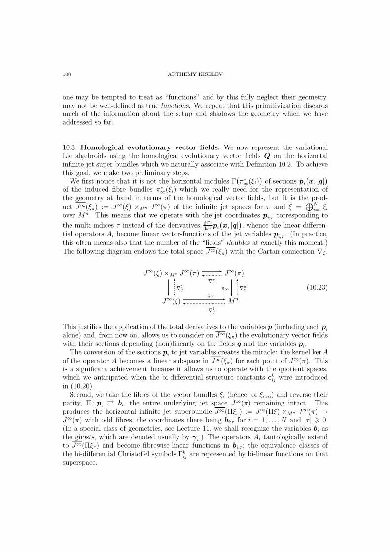
108 ARTHEMY KISELEV

one may be tempted to treat as “functions” and by this fully neglect their geometry,may not be well-defined as true functions. We repeat that this primitivization discardsmuch of the information about the setup and shadows the geometry which we haveaddressed so far.

10.3. Homological evolutionary vector fields. We now represent the variationalLie algebroids using the homological evolutionary vector fields Q on the horizontalinfinite jet super-bundles which we naturally associate with Definition 10.2. To achievethis goal, we make two preliminary steps.

We first notice that it is not the horizontal modules Γ(π∗∞(ξi)

)of sections pi

(x, [q]

)

of the induced fibre bundles π∗∞(ξi) which we really need for the representation ofthe geometry at hand in terms of the homological vector fields, but it is the prod-uct J∞(ξπ) := J∞(ξ) ×Mn J∞(π) of the infinite jet spaces for π and ξ =

⊕Ni=1 ξi

over Mn. This means that we operate with the jet coordinates pi;τ corresponding to

the multi-indices τ instead of the derivatives d|τ |

dxτ pi(x, [q]

), whence the linear differen-

tial operators Ai become linear vector-functions of the jet variables pi;τ . (In practice,this often means also that the number of the “fields” doubles at exactly this moment.)The following diagram endows the total space J∞(ξπ) with the Cartan connection ∇C,

J∞(ξ)×Mn J∞(π)-

.....∇πC

....... J∞(π)

J∞(ξ)?

∇ξC

6........ ξ∞ -

..................∇ξC

......... Mn.

π∞

?∇πC

6........

(10.23)

This justifies the application of the total derivatives to the variables p (including each pialone) and, from now on, allows us to consider on J∞(ξπ) the evolutionary vector fieldswith their sections depending (non)linearly on the fields q and the variables pi.

The conversion of the sections pi to jet variables creates the miracle: the kernel kerAof the operator A becomes a linear subspace in J∞(ξπ) for each point of J∞(π). Thisis a significant achievement because it allows us to operate with the quotient spaces,which we anticipated when the bi-differential structure constants ckij were introducedin (10.20).

Second, we take the fibres of the vector bundles ξi (hence, of ξi,∞) and reverse theirparity, Π: pi bi, the entire underlying jet space J∞(π) remaining intact. Thisproduces the horizontal infinite jet superbundle J∞(Πξπ) := J∞(Πξ) ×Mn J∞(π) →J∞(π) with odd fibres, the coordinates there being bi;τ for i = 1, . . . , N and |τ | > 0.(In a special class of geometries, see Lecture 11, we shall recognize the variables bi asthe ghosts, which are denoted usually by γi.) The operators Ai tautologically extendto J∞(Πξπ) and become fibrewise-linear functions in bi;τ ; the equivalence classes ofthe bi-differential Christoffel symbols Γkij are represented by bi-linear functions on thatsuperspace.


Theorem 10.6 ([50]). Whatever representatives in the equivalence classes of the bi-differential symbols Γkij be taken, the odd-parity evolutionary vector field

Q = ∂(q)∑N

i=1 Ai(bi)−

1

2

N∑

k=1

∂(bk)∑N

i,j=1 Γkij(bi,bj)

(10.24)

is homological :

Q2 = 0 (mod

N∑

k=1

∂(bk)ϕk(b⊗b⊗b) |

N∑

k=1

Ak(ϕk) = 0).

Example 10.7. Let us give at once a minimally possible nontrivial illustration. Theoperator = ux+ 1

2ddx

for the Liouville equation uxy = exp(2u) specifies the differential

Q = ∂(u)(b) + ∂

(b)bbx

;

the equality of the even velocity bbx of the odd variable b to the respective velocity inthe field (see Exercise 9.5 on p. 88)

Q = ∂(w)

AKdV2 (b)

+ ∂(b)bbx

for the Korteweg–de Vries equation wt = −12wxxx + 3wwx is no coincidence !

We prefer to prove the theorem straightforwardly, not passing from many arguments ofmany operators to the tall sections of wide operators, see (10.18). This attests that thenature of the variables bi at different i’s may be entirely uncorrelated.

Proof. The halved anticommutator 12[Q,Q] = Q2 of the odd vector field Q with itself

is an evolutionary vector field. In this anticommutator, the coefficient of ∂/∂q, whichdetermines the coefficients of ∂/∂qσ at all |σ| > 0, is equal to

∂(q)∑N

i=1Ai(bi)

( N∑

j=1

Aj(bj))−

1

2

N∑

k,ℓ=1

δℓk · Aℓ

( N∑

i,j=1

Γkij(bi, bj))

;

the evaluation (8.2) of this coefficient at any two “tall” sections p1 and p2 gives zeroby the definition of the symbols Γkij.

Second, let us consider the Jacobi identity for the Lie algebra of evolutionary vectorfields with the generating sections belonging to the images of the operators A1, . . ., ANviewed as the fibrewise-linear functions on the total space of the bundle J∞(ξπ) →J∞(π):

0 =∑

(imn)

[Ai(pi),

∑

k

Ak(Γkmn(pm,pn)

)]

=∑

(imn)

∑

k

Ak

∂

(q)Ai(pi)

(Γkmn(pm,pn)

)+∑

ℓ

Γkiℓ(pi,Γ

ℓmn(pm,pn)

),

110 ARTHEMY KISELEV

where we have relabelled the indices ℓ k in the second sum,

= −∑

(imn)

∑

k

Ak

−∂

(q)Ai(pi)

(Γkmn(pm,pn)

)+∑

ℓ

Γkℓi(Γℓmn(pm,pn),pi

). (10.25)

Thirdly, the velocity of each odd variable bk induced by the (for convenience, not halved)anticommutator [Q,Q] = 2Q2 is obtained as follows,

−∂(q)∑N

i=1Ai(bi)

(∑

m,n

Γkmn(bm, bn))

+1

2

N∑

ℓ=1

∂(bℓ)∑m,n

Γℓmn(bm,bn)

(∑

j,i

Γkji(bj , bj))

= −∂(q)∑N

i=1Ai(bi)

(∑

m,n

Γkmn(bm, bn))

+1

2

∑

ℓ,i

Γkℓi

(∑

m,n

Γℓmn(bm, bn), bi

)−

1

2

∑

i,ℓ

Γkiℓ

(bi,∑

m,n

Γℓmn(bm, bn))

=∑

i,m,n

−∂

(q)Ai(bi)

(Γkmn(bm, bn)

)+

N∑

ℓ=1

Γkℓi(Γℓmn(bm, bn), bi

).

We notice that the extra sum over the three cyclic permutations of each fixed set ofthe indices i, m, and n does not produce any change of the signs because the cyclicpermutations (of the respective three odd b’s) are even. Consequently, by taking thesum of all possible Jacobi identities (10.25), we conclude that the sought-for coefficientis equal to

=1

3

∑

i,m,n

∑

(imn)

. . .

= 0 (mod ϕ = (ϕ1, . . . , ϕN) |N∑

k=1

Ak(ϕk) = 0).

This completes the proof.

Remark 10.6. The above construction of the homological vector field Q in absence ofthe equations of motion but with an a priori given collection A1, . . ., AN of genera-tors (10.24) for the infinitesimal transformations of the model patterns upon the con-struction of nontrivial gauge theories with the zero action functional and the prescribednontrivial gauge group, see [9, 110].

In the next lecture we shall consider the general case of gauge models[5] with a possiblynontrivial action S(x, [q]) and associate the evolutionary BRST-differentials Q and theBV-differentials D with such systems; these homological vector fields D are themselvesHamiltonian with respect to the full BV-action S = S + . . . such that D = [[S, · ]].

Likewise, the correspondence QP = [[P , ·]] between the (non)commutative variationalPoisson bi-vectors P satisfying the classical master-equation [[P ,P ]] = 0 is a regularsource of the homological vector fields (see Lectures 8–9). Let us notice further thatthese fields are Hamiltonian: indeed, the bi-vector P = 1

2〈b, A(b)〉 then stands as the

Hamiltonian functional that specifies the dynamics via the odd Poisson bracket [[ , ]].


We conclude this lecture with a convenient criterion[49] which states whether a givendifferential operator A is Hamiltonian and endows the space H

n(π) of functionals on

J∞(π) with a Poisson bracket.

Theorem 10.7. A skew-adjoint linear total differential operator A : p ∈ P 7→ ∂(q)A(p)

with involutive image is Hamiltonian if and only if

QA(P) = 0 ∈ Hn(Πππ),

where QA is the odd-parity vector field (10.4) on J∞(Πππ) and P = 12〈b, A(b)〉 is the

bi-vector.

Remark 10.7. The equality A = −A† of the mappings A : P → κ(π) and A† : κ(π)→ P

uniquely determines the domain P = κ(π) of A. We now see that the “only if” part ofthe assertion is Exercise 9.3 on p. 88 combined with Problem 9.3.

Proof. Because the operator A is skew-adjoint, the bi-vector P = 12〈b, A(b)〉 is well

defined. By definition, put QA = ∂(q)A(b)−

12∂

(b)b,bA

, where the Christoffel symbol , A

is such that ∂(q)A(p1)(A)(p2) − ∂

(q)A(p2)(A)(p1) = A(p1,p2A) for any sections p1,p2 ∈

κ(π). We note that if , A ≡ 0, there is nothing to prove (see Exercise 9.4 on p. 88).From now on, we suppose that , A 6≡ 0.

Using the Leibniz rule, we deduce that

0 = QA(P) = 12〈−1

2b, bA, A(b)〉 − 1

2〈b, ∂

(q)A(b)(A)(b)〉+ 1

2〈b, 1

2A(b, bA)〉,

where we integrate by parts in the first term of the right-hand side and obtain

∼= 12·(−1

2〈b, A(b, bA)〉+ 〈b,−∂

(q)A(b)(A)(b) + 1

2A(b, bA)〉

).

The evaluation (8.2) of the underlined factor in the second coupling at any two covectorsyields zero so that there only remains

= (−12) · 〈b, A(1

2b, bA)〉.

By the hypothesis of the theorem, the value of this tri-vector at any three covectors p1,

p2, and p3 ∈ κ(π) is equal to

−1

2·∑

〈p1, A(p2,p3A)〉 = 0 ∈ Hn(π). (10.26)

We claim that the sum (10.26) is zero if and only if A is a Hamiltonian operator (i. e.,whenever it induces the Poisson bracket , A which satisfies the Jacobi identity).

Indeed, define a bi-linear skew-symmetric bracket , A for any Hi,Hj ∈ Hn(π) by

the rule

Hi,HjA :=⟨δHi/δq, A(δHj/δq)

⟩∼= ∂

(q)A(δHj/δq)(Hi).

112 ARTHEMY KISELEV

Now let H1, H2, and H3 ∈ Hn(π) be three arbitrary functionals and put pi(x, [q]) =

δHi/δq for i = 1, 2, 3. Then the left-hand side of the Jacobi identity for the brack-et , A is, up to a nonzero constant, equal to∑

∂(q)A(p1)〈p2, A(p3)〉

=∑

(〈∂

(q)A(p1)(p2), A(p3)〉+ 〈p2, ∂

(q)A(p1)

(A)(p3)〉+⟨p2, A

(∂

(q)A(p1)(p3)

)⟩). (10.27)

Let us integrate by parts in the last term of the right-hand side; at the same time,

using the property ℓ(q)p2

= ℓ(q)†p2

of the exact covector p2 = δH2/δq (we assume thatthe topology of the bundle π matches the hypotheses of the Helmholtz theorem 5.1 onp. 55), we conclude that the first term in the right-hand side of (10.27) equals

〈ℓ(q)p2

(A(p1)

), A(p3)〉 = 〈ℓ(q)†

p2

(A(p1)

), A(p3)〉 ∼= 〈ℓ(q)

p2

(A(p3)

), A(p1)〉 =

= 〈∂(q)A(p3)(p2), A(p1)〉.

Continuing the equality from (10.27), we have

∼=∑

(〈p2, ∂

(q)A(p1)(A)(p3)〉+ 〈∂

(q)A(p3)(p2), A(p1)〉 − 〈∂

(q)A(p1)(p3), A(p2)〉

).

The 3 + 3 underlined terms cancel in the sum, whence we obtain the equality

=∑

〈p1, ∂(q)A(p3)(A)(p2)〉 =

1

2

∑

〈p1, ∂(q)A(p3)

(A)(p2)− ∂(q)A(p2)(A)(p3)〉

= −1

2·∑

⟨p1, A

(p2,p3A

)⟩.

By (10.26), this expression equals zero.37 Therefore, the Jacobi identity for the brack-et , A holds, whence the operator A is Hamiltonian. The proof is complete.

Remark 10.8. Theorem 10.7 converts the quadratic equation [[P ,P]] = 0⇔ (QP)2 = 0to the bi-linear condition QA(P) = 0 upon the bi-vector P and the Q-structure for theinfinite jet superspace J∞(Πππ), which is endowed with the odd Poisson bracket [[ , ]],c. f. [1].

Problem 10.1 ([20]). Prove that the variational derivative δ/δq and a Hamiltoniandifferential operator A establish the Lie agebra homomorphisms

(Hn(π), , A

)−→

(κ(π), [ , ]A

)−→

(κ(π), [ , ]

).

Problem 10.2. By a direct calculation — i. e., not appealing to formula (9.11) andthe property (QP)2 = 0 of the Poisson bi-vectors P induced by that factorization, —demonstrate that the odd-parity evolutionary vector fields Q are the differentials for

37By the substitution principle (which is Problem 9.2), if such an expression vanishes for the exact

covectors pi = δHi/δq, then it vanishes for all sections pi ∈ κ(π).


each root system of a semisimple complex Lie algebra of rank two and the generator of symmetries for the associated nonperiodic 2D Toda chain. (The formulas for theanchors and the Christoffel symbols , are contained in [64].)

Problem 10.3. Consider the generator DA = d + [A, · ] of the gauge symmetriesfor the Yang–Mills equations DA ∗ DA(A) = 0, where A = Ai dx

i is the connectionone-form (containing the fields Ai) in the principal G-bundle over M3,1 and ∗ is theHodge structure on the Minkowski space-time M3,1 (e. g., let G = U(1), G = SU(2), orG = SU(3)). Assume that the Lie algebra g of the Lie group G is complex semi-simple.

Suppose first that the image of DA is involutive and, were it indeed so, show that

• the total differential order of the bi-differential Christoffel symbol , DAmust

be equal to zero;• the differential order of the coefficients of the Christoffel symbol must be equal

to zero;• moreover, the coefficients of , DA

can not depend on the unknown vari-ables A;• but also, in view of the invariance of the Yang–Mills theory under translations

along the base M3,1, those coefficients can not depend on the points x ∈M3,1.

Recall further that, by construction, the gauge parameters p ∈ P1 belong to the hor-

izontal module P1 ≃ g ⊗C∞(M3,1) F(π), where π is the fibre bundle over M3,1 for theconnection fields A, but let us identify g∗ ≃ g by using the Killing form of the semi-simple complex Lie algebra g.• Prove that the image of the gauge symmetry generator DA is closed under com-mutation and the entries of the Christoffel symbol , DA

are equal to the structureconstants of the Lie algebra g.

114 ARTHEMY KISELEV

11. BRST- and BV-formalism

In this lecture we study the geometry of the Becchi–Rouet–Stora–Tyutin[11] (BRST) andBatalin–Vilkovisky[8] (BV) approach to the quantisation of the Euler–Lagrange gaugemodels with the action S and the structure group G. The main element of this techniqueis the representation of Lie algebroids over infinite jet spaces J∞(π) in terms of thehomological evolutionary vector fields Q, which we introduced in the previous lecture.The BRST technique resolves[4, 39] the algebra of gauge-invariant observables (i. e., thefunctions or functionals which remain unchanged under the gauge transformations) asthe zero cohomology of the complex endowed with the differential Q. In turn, the BV-formalism extends the domain of definition for the differential Q to the Whitney sumover J∞(π) of the induced fibre (super-)bundles containing not only the unknowns q(which are the gauge fields) and the field-dependent gauge parameters p, but also theequations of motion, the (higher generations of the) Noether identities, and the elementsof the modules which are dual to the equations and all such syzygies (see Lecture 2).By reversing the parity of the fibres in, roughly speaking, a half of the horizontal jetspaces for these induced bundles, we complete the classical BV-zoo[7, 29, 108] which isinhabited by the (anti)fields, (anti)ghosts, and possibly, the extra pairs of the variableswhich stem from the higher generations of the syzygies.

It is now clear that the gauge systems carry the excessive degrees of freedom which arenot essential in the study of the physics described by such models. Firstly, all objects arelittered with the identically-zero elements that contain the Noether identities. Second,it is the motion along the gauge orbits that yields the physically equivalent states.Neither of the two factors contributes to the values of the observables from F(π)G orHn(π)G. (Again, the two emerging sub-theories for the differential functions and the

integral functionals do and, respectively, do not distinguish between the points of thesource manifold Mn. But we are free to choose the right concept: a field theory over thespace-time votes for the first option while the theory of strings within the space-timesets the preference for the other.) It is our intermediate goal to introduce a cohomologytheory whose zeroth term would be the space of the observables of our choice. Sucha theory will allow us to deal with the on-shell defined gauge-invariant objects stayingoff-shell in the jet space and not taking care about fixing the gauge.[36, 94]

For consistency, let us recall from Lecture 6 some basic facts about the Euler-Lagrangegauge systems. We know that every Euler–Lagrange system EEL =

F = δS/δq = 0 |

S ∈ Hn(π)

contains as many equations as there are unknowns q. By convention,such equations Fi = 0 are labelled by the respective fields qi; let us remember that the

horizontal module P0 of the sections F is then P0 ≃ κ(π).The gauge systems do admit the differential constraints (the syzygies or the Noether

identities) between the equations of motion,

Φ(x, [q], [F (x, [q])]) ≡ 0 on J∞(π), Φ ∈ P1 = Γ(ξ1ξπ

).

The relations Φi+1(x, [q], [F ], [Φ], . . . , [Φi]) ≡ 0 between the relations, whenever validfor all sections s ∈ Γ(π) identically in q, F , . . ., Φi−1 (here Φ0 = F ∈ P0), give rise topossibly several but always finitely many generations of the horizontal modules Pi ∋ Φi

for i > 0.


As in Lecture 6, we assume that the given action functional S determines the sys-tem EEL = F = 0 of equations of motion with one generation of the constraintsΦ(x, [q], [F ]) = 0 and that there are no further relations between the already knownones. However, if a given model is reducible — i. e., there is at least one more gen-eration of the syzygies Φ2

(x, [q], [F ], [Φ]

)≡ 0 ∈ P2 between the Noether identities

Φ ≡ 0 ∈ P1, — then each new generation of the relations, which are stored in the

suitable horizontal modules Pi, i > 2, gives rise to the four neighbours:38 Pi, ΠPi, Pi,

and ΠPi.By the Second Noether Theorem 6.1, the relations Φ

(x, [q], [F ]

)= 0 between the

equations Fj = 0, 1 6 j 6 m, yields the linear total differential operator A : P1 →sym EEL that generates the gauge symmetries of the Euler–Lagrange system EEL. Suchsymmetries are parametrized by arbitrary field-dependent gauge parameters p

(x, [q]

)∈

P1.We assume further that the operator A can be extended to the operator that takes

values in the larger space κ(π) ⊇ sym EEL; such extensions could in principle involvethe improper symmetries which vanish on-shell. (However, let us emphasize that somegauge symmetries may be Noether and some Noether symmetries may be gauge, still

the two concepts are distinct in general.) Let the columns A1, . . ., AN : P1 → κ(π)of the operator A be the entire collection of the gauge symmetry generators for thesystem EEL. For the sake of clarity, we assume the off-shell validity of the Berends–Burgers–van Dam hypothesis[14] about the collective commutation closure for the imagesof these operators, see (10.11). In other words, we postulate that the extensions of thegauge symmetry generators, which take their values in sym EEL, are such that the im-proper symmetries do not occur explicitly in the off-shell involutivity condition (10.17).

Then the parity-reversed arguments b ∈ ΠP1 = Γ(π∗∞(Πξ1)

)are known as the ghosts,

usually denoted by γ. The even elements of the dual module P1 are39 the antighosts γ†.In the following diagram we summarize the notation and interpret the objects at handin terms of the BRST- and BV-theory:[8, 26]

ghosts - γ = b ∈ ΠP1 γ† ∈ P1 antighosts

gauge parameters - ǫ = p ∈ P1

Π6

? ∗

〈 , 〉- Φ[F ] ∈ P1

id

?

6

Noether identities

q† ∈ ΠP0 antifields

Noether symmetries - ϕL.= ψ ∈ κ(π) ≃ P0

∗

〈 , 〉- F ∈ P0 ≃ κ(π)

Π6

? usual identification.

38Thus, each generation yields the canonically conjugate, 〈 , 〉-dual pair of the higher ghosts ci ∈

(Π)Pi and the higher antighosts c†i ∈ (Π)Pi of opposite parity, see the diagram below.

39We do not fix any metric on the base manifold Mn and therefore not grasp the subtle differencebetween the commonly accepted transcripts q† vs q∗ for the antifields and γ† vs γ∗ for the antighosts(see, e. g., [16]). For the same reason, in this course we do not pay any particular attention to theupper or lower location of the indices.

116 ARTHEMY KISELEV

Passing to the horizontal jet bundle J∞(π∗∞(Πξ1)

)over J∞(π), we then apply Theo-

rem 10.6 and construct the odd evolutionary vector field Q. This is the Becchi–Rouet–

Stora–Tyutin (BRST-) differential.[11] The variational Lie algebroid which is encodedby the evolutionary differential Q is the gauge algebroid.

This generalization of the odd cotangent covering ΠT∗J∞(π) over the initial jet spaceJ∞(π) is again endowed with the odd Poisson bracket [[ , ]] (i. e., the Schouten bracketor the antibracket, see Lecture 8). Likewise, the action S(x, [q]) for the equation ofmotion E∞EL ⊆ J∞(π) can be extended to the full BV-action S = S+. . . that satisfies theclassical master equation [[S,S]] = 0. The new functional induces the BV-differentialD = [[S, · ]] that incorporates Q as the “longitudinal” component along the gaugeorbits.

Let us first inspect the (co)vectorial nature of the objects at hand (by definition,

the evolutionary fields ∂(q)ϕ are vectors). This is essential for the future use of Dirac’s

convention about the bra- covectors 〈 | and -ket vectors | 〉 in the definition of theantibracket by using the full set of the BV-variables which are now at our disposal.

Exercise 11.1. Consider the pair of variables q ←→ q† = F †, where Π: F F †; theodd objects q† are called the antifields. Show that under a reparametrization40 of thevariables q, the variation δq† is an odd vector (c. f. [2, §37]).• Second, let Φ ∈ P1 be the column of the Noether identities and consider the corre-sponding pair γ ←→ γ†. Show that the even antighost γ† transforms as the coefficientsof a vector, whence δγ† is a covector, and that the variation δγ is a vector for the〈 , 〉-dual odd ghost γ.

This yields the odd-parity symplectic structure

ω = δq ∧ δq† + δγ† ∧ δγ

on the Whitney sum of the respective horizontal jet (super-)spaces and fixes the choiceof the signs in the antibracket (see [120] and, e. g., [37, 116])

[[ξ,η]] =⟨−→δξ ∧

←−δη⟩,

which straightforwardly extends to all the generations i = 1, . . . , λ of the ghost-antighostpairs.41

40We remark that this exercise is concerned with the identification of the left-hand sides of the Euler–Lagrange equations as variational covectors F δq; the variables q could describe, e. g., the coefficientsof the connection one-form in a principal fibre bundle over the manifold Mn so that the vector bundle πinvolves as the unknowns the components of a covector !

41Likewise, the odd Laplacian is

∆BV =

−→δ

δq

←−δ

δq†+

−→δ

δγ†

←−δ

δγ.


We have that [[ξ,η]] =

(−→δξδq〈δq, δq†〉

←−δη

δq†−

−→δξ

δq†〈δq, δq†〉

←−δη

δq

)+( −→δξδγ†〈δγ†, δγ〉

←−δη

δγ−

−→δξ

δγ〈δγ†, δγ〉

←−δη

δγ†

)

=

[−→δξ

δq·

←−δη

δq†−

−→δξ

δq†·

←−δη

δq

]+

[ −→δξ

δγ†·

←−δη

δγ−

−→δξ

δγ·

←−δη

δγ†

].

The main miracle of the Batalin–Fradkin–Vilkovisky theory is the existence of themaster-action[40, 74]

S = S + 〈q†, Ak(γk)〉 −1

2

⟨Γkij(γi,γj),γ

†k

⟩+ 〈correction terms〉 (11.1)

that

(1) extends the action S(x, [q]) ∈ Hn(π) for the equations of motion and

(2) satisfies the classical master equation

[[S,S]] = 0. (11.2)

The possible necessity to introduce the correction terms of higher polynomial orders inthe odd variables q† and γ or their derivatives —with an also possible dependence on[γ†] and the higher ghost–antighost pairs— is legitimate whenever the coefficients ofthe bi-differential Christoffel symbols Γkij explicitly depend on the fields q.

Exercise 11.2. Show that no correction terms appear in the BV-action (11.1) for theYang–Mills equations with S = const ·

∫〈∗F ∧ F〉, see Problem 2.5 and 10.3, and then

verify the classical master equation (11.2) by a direct calculation.

Remark 11.1. The theory guarantees the existence of a solution S to the classical masterequation (11.2) in the form of a power series in the (derivatives of the) BV-variables q†,γ ↔ γ†, and the higher ghost–antighost pairs cα ↔ c†α. Such solution S = S + . . . canbe obtained perturbatively because no obstructions appear at each step from a degreeℓ to ℓ+ 1. In this sense, equation (11.2) is formally integrable.

Let us notice, however, that the series S truncates after a finite number of stepsfor many relevant systems (see Exercise 11.2). At the same time, we emphasize thata possible presence of infinitely many derivatives of unbounded orders, which is incontrast with our earlier convention about the differential functions (see Lecture 1) stilldoes not imply that the theory becomes nonlocal, i. e., that it involves the values ofcertain sections at more than one point of the base Mn. Indeed, the formal powerseries (11.1) can be divergent almost everywhere.

Definition 11.1. The Batalin–Vilkovisky differential is the evolutionary vectorfield DBV which acts by the rule

DBV( · ) ∼= [[S, · ]];

the domain of definition of the right-hand side is the space of functionals that dependon all the BV-variables.

Exercise 11.3. Show that DBV = Q+ . . . (in fact, the dots stand for the Koszul–Tate

differential, which captures the Noether identities and the higher generations of thesyzygies, plus the correction terms).

118 ARTHEMY KISELEV

By construction, the functionals F and F+ε[[S,G]] now describe the same physics forany G: indeed, we place both functionals in the same cohomology class within H0

[[S, · ]].

Remark 11.2. Strictly speaking, the homological evolutionary vector field DBV and thedifferential [[S, · ]] are defined on non-coinciding spaces. Indeed, the domain of definitionof DBV is the category of all modules of sections of the induced bundles whose base isthe total space for the Whitney sum of the horizontal jet spaces over J∞(π) with theBV-coordinates along their fibres. For example, the application of DBV to a function

qxq†(γ†)2γxxx is well defined but the differential [[S, · ]] can act only on the functional∫

qxq†(γ†)2γxxx dx.

Remark 11.3. The BRST-field Q and the BV-field DBV were introduced formally bypostulating that they are differentials. Unfortunately, it follows from nowhere thatthese evolutionary vector fields should at the same time be geometric, i, e., why thevalues of the velocities of the BV-coordinates (such as the ghosts γ) on true sectionsγ = Πp

(x, [q]

)of the horizontal bundles over J∞(π) do coincide — up to the necessity

to recover the standard summands in (10.20) — with the velocities

L∂(q)A(Πp(x,[q]))

(Πp(x, [q])

)

of those sections, induced by the evolution q = A(γ) on the fields q, c. f. Lemma 8.1on p. 82.

Exercise 11.4. Show that the formal evolutionary vector fields (10.24) are geometricfor all Hamiltonian operators (and from this deduce that Lemma 8.1 calculates therespective bi-differential Christoffel symbols).

Exercise 11.5. Suppose that the above conjecture is true and thus, all the homologi-cal evolutionary vector field realizations Q of variational Lie algebroids are geometric.Prove that every skew-adjoint linear total differential operator with involutive image ing(π) = (κ(π), [ , ]) is a Hamiltonian operator (c. f. Theorem 10.7).

The Batalin–Fradkin–Vilkovisky method is a tool for the quantisation of gaugesystems.[37] As usual, all the dependent variables become formal power series in thePlanck constant ~; in particular, the full BV-action is now the formal power series S~.

Exercise 11.6. List, count their number, and classify the conceptual difficulties of thetheory which one encounters during the derivation of the quantum master-equation

i~∆BVS~ −12[[S~,S~]] = 0

from the equality

∆BV

(exp

(i

~S~

))= 0,

which itself follows from the postulate

〈1〉 =

∫exp

(i

~S~(x, [q])

)[Dq]

for the Feynman path integral.


Finally, let us recall from [16] a remarkable link between the application of the Batal-in–Vilkovisky method to a nonlinear Poisson sigma model (c. f. [1, 117]) and to thecalculation of Feynman’s path integrals and, on the other hand, the Kontsevich defor-mation quantisation of the Poisson brackets on usual manifolds,[68] which we addressedin Lecture 9.

Let D be a disc in R2 and Nm be a Poisson manifold endowed with the Poisson bi-vector P ij . The fields in this model are the mappings X : D → Nm and the differentialone-forms η on D taking values in the pull-back under X of the cotangent bundle overNm; it is also supposed that at the boundary ∂D of the disc those forms vanish on allvector fields which are tangent to the boundary.

The action of the model is

S ([X], [η]) =

∫

D

(ηi(u) ∧ dXi(u) + 1

2P ij∣∣X(u)

(ηi(u) ∧ ηj(u)) du). (11.3)

Let 0, 1, and ∞ be any three cyclically ordered points on the boundary ∂D and f, g ∈C∞(N) be functions (i. e., the Hamiltonians). Then the star-product f ⋆ g is the semi-classical expansion of the path integral:

(f ⋆ g)(x) =

∫

X(∞)=x

f(X(1))g(X(0)) exp

(i

~S([X], [η])

)[DXDη]. (11.4)

Problem 11.1. Calculate the Noether identities Φ, gauge symmetry generators A, bi-differential Christoffel symbols , A, the BRST evolutionary vector field Q, the fullBV-action S, and the Batalin–Vilkovisky differential DBV for the Poisson sigma modelwith action (11.3) (see also [30]).• Calculate the path integral (11.4) and re-derive the Kontsevich formula for the star-product f ⋆ g as the sum over graphs.

Problem 11.2. Inspect the induced transformation of the (BRST-) homological vectorfield Q under the cylindric symmetry reduction of the Yang–Mills equation to thenonpreriodic 2D Toda chains (c. f. [88]), and reveal the origin of the integrals w1, . . .,wr for these exponential-nonlinear hyperbolic equations[112] in terms of the geometry ofthe full Yang–Mills models.

120 ARTHEMY KISELEV

12. Deformations of nonlocal structures

This is the last lecture in the course: in it we bring together the concepts of gaugeinvariance and nonlocalities. Namely, we analyse the geometry of non-abelian coveringsover differential equations and study the deformations of these structures. Our attentionis focused on finding parametric families of

• Backlund (auto)transformations between equations, and• Lie-algebra valued zero-curvature representations for nonlinear systems.

Backlund transformations allow us to produce new –e. g., multi-soliton– solutions fromknown ones (for instance, starting from very simple sections or from the solutions whichdescribe a smaller number of solitons). On the other hand, the technique of Lax pairs,which is furthered to the notion of zero-curvature representations, allow us to solvethe Cauchy problems for nonlinear partial differential equations by using the inversescattering transform. A detailed exposition of the kinematic integrability approachwould go far beyond the frames of our first acquaintance with it; indeed, here we onlyhighlight its most prominent elements, placing them in the context of the already knownmaterial.

The notion of covering, which was introduced in Lecture 7, is omnipresent here. Inthe first part of this lecture we study Backlund (auto)transformations, which are thecorrelated pairs of coverings. Next, we address Gardner’s deformations from a similarperspective and inspect how they are naturally generalized to the construction of gaugecoverings in terms of flat connections in the principal fibre bundles over differentialequations.

12.1. Backlund (auto)transformations. Intuitively, a Backlund transformation be-

tween two equations E1 ⊆ Jk1(π1) and E2 ⊆ Jk2(π2) is a system E of differential relationswhich are imposed on the respective unknowns u1 and u2 in E1 and E2 and which aresuch that if a section s1 ∈ Γ(π1) solves the first equation E1 and two sections s1 and s2

satisfy those relations E simultaneously, then s2 ∈ Γ(π2) is a solution of the equationE2, and vice versa.

Example 12.1. The Cauchy–Riemann equations v1y = v2

x, v1x = −v2

y determine the

Backlund autotransformation for the Laplace equation on R2 (here E1 = ∆v1 = 0and E2 = ∆v2 = 0 are two copies of the Laplace equation).

Definition 12.1. Let Ei ⊆ Jki(πi), i = 1, 2, be two formally integrable differential

equations, E∞i be their prolongations, and τi : E → E∞i be the coverings with the same

total space E . Then the diagram B(E ; τi; Ei)

Eτ1ւ

τ2ց

E∞1 E∞2

(12.1)

is called a Backlund transformation between the equations E1 and E2. Diagram (12.1)is called a Backlund autotransformation for the system E if E∞1 ≃ E

∞2 ≃ E

∞.

Exercise 12.1. Consider the covering τ+ of the Korteweg–de Vries equation w+t =

−12w+xxx + 3w+w+

x by the modified KdV equation mt = −12mxxx + 3m2mx, where the


projection τ+ is determined by the Miura substitution w+ = 4m2 + 2mx. Notice thatthe modified KdV equation EmKdV admits the discrete symmetry µ : m 7→ −m. Denoteby τ− = τ+ µ : EmKdV → E

∞KdV another covering over the second copy of the Korte-

weg–de Vries equation EKdV upon the unknown w−. Then B(EmKdV; τ+, τ−; EKdV) isa Backlund autotransformation for the equation EKdV. By eliminating the variable maltogether, derive the relations between the unknowns w+ and w− and their derivatives.

Remark 12.1. We shall consider only those pairs of fibre bundles π1 and π2 which alsohave the common base Mn, assuming that it remains intact under the morphisms ofbundles. We thus exclude from the further consideration those transformations whichswap or mix the independent variables on the base with the unknowns along the fibres(e. g., as it happens in the reciprocal transformations).

Exercise 12.2. Show that every dispersionless two-component system ut = f(u) · uxwith two independent variables can be made linear by the hodograph transformationu1(t, x), u2(t, x) 7→ t(u1, u2), x(u1, u2).

Remark 12.2. A Backlund autotransformation B(E ; τi; E) for an equation E = F = 0

induces the tangent Backlund autotransformation TB(TE ; τi ⊗ Tτi; TE) between thetangent coverings TE over the two copies of E (the definition of TE , see Lecture 7, isbased on the introduction of the “linearized” variables U on top of the unknowns u so

that the linearized equations ℓ(u)F (U) = 0 hold).

Definition 12.2. The recursion transformation for symmetries ϕ ∈ ker ℓ(u)F

∣∣∣E

of an

equation E = F = 0 is a Backlund autotransformation for the linearized system

ℓ(u)F (U) = 0.

We conclude that an equation E does admit a recursion transformation for its sym-metries if there is a Backlund autotransformation for solutions of E .

Let us now study the construction of Backlund (auto)transformations in more detail.

Let τi : Ei → E∞i be two coverings (i = 1, 2) and µ : E1 → E2 be a diffeomorphism of

manifolds with distributions (i. e., the tangent mapping µ∗ : Cτ1 → Cτ2 is an isomorphism

of the Cartan distribution at all points of E1), though not necessarily a morphism ofthe coverings which would transform the underlying equations one into another andpreserve the structure of the nonlocal fibres over them. Rather, the diffeomorphismµ could swap the fibre variables in π1 with the nonlocal variables along the fibre of

τ1 : E → E∞1 ; this guarantees that the resulting transformation of solutions to E1 does

not amount to a mere finite symmetry.[43] Then the diagram B(E1; τ1, τ2 µ; Ei) is aBacklund transformation between the equations E1 and E2.

Example 12.2. Consider the Liouville equation ELiou = uxy = exp(2u) and construct

the family of one-dimensional coverings τλ : Eλ → E∞Liou over it: let us extend the total

derivatives

d

dx=

d

dx

∣∣∣∣ELiou

+ ux∂

∂u,

d

dy=

d

dy

∣∣∣∣ELiou

+ uy∂

∂u,

[d

dx,

d

dy

]= 0

122 ARTHEMY KISELEV

by setting the derivatives of the nonlocal variable u = u(λ) as follows:

ux = ux + exp(−λ) · exp(u+ u),

uy =− uy + 2 exp(λ) · sinh(u− u).(12.2)

Let the diffeomorphism µ be the swapping u u of the fibre variable u in ELiou and thenonlocality u combined with the involution x 7→ −x and y 7→ −y. Then the diagram

B(Eλ; τλ, τλ µ; ELiou) is a Backlund autotransformation for the Liouville equation. The

relations in Eλ are, obviously,

(u− u)x = exp(−λ) · exp(u+ u),

(u+ u)y = 2 exp(λ) · sinh(u− u).(12.3)

For each λ ∈ R, the unknown u satisfies the equation uxy = exp(2u) whenever u solvesuxy = exp(2u), and vice versa.

Exercise 12.3. Construct the one-parametric families of Backlund (au-to)transformations for all possible choices of a pair from the following list:

• the Liouville equation uxy = exp(2u),• the wave equation vxy = 0, and• the scal+-Liouville equation Υxy = exp(−2Υ) that describes the conformal met-

rics42 of positive constant Gauss curvature K = +1.

Backlund (auto)transformations become the powerful generators of exact solutions to

nonlinear systems when they appear in families Bλ(Eλ; τλi ; Ei). In Lecture 7 we revealed

a mechanism for the construction of families of coverings over differential equations:Suppose that ϕ is a τ1-shadow that preserves E1 for all values of the nonlocalities butdoes not lift to a true τ1-nonlocal symmetry of the equation Eλ=λ0 in the coveringτ1. Consequently, this shadow spreads the Cartan differentials of the nonlocalities toa one-parametric family, which determines the law of deformation for the coveringequations Eλ.

Exercise 12.4. Show that it is the scaling symmetry

X = −x∂

∂x+ y

∂

∂y+ . . . (find this lifting explicitly !)

of the Liouville equation that generates the one-parametric family of coverings (12.2);here λ is the natural parameter along the flow Aλ = exp(λX).

Exercise 12.5. By noticing that the Galilean symmetry of the Korteweg–de Vriesequation does not lift to the modified KdV equation (see Exercise 12.1), construct aone-parametric family of Backlund autotransformations for the KdV equation.

Remark 12.3. In the literature, the natural parameter λ along such integral trajectoriesoften appears in disguise in the resulting families of the Backlund transformations: it

is k = exp(λ) but not λ itself which is taken to mark the relations Bλ(Eλ; τλi ; E∞i ).

42Backlund (auto)transformations were historically first discovered for the sine–Gordon equation inthe context of propagation of the pseudospherical surfaces of negative Gauss curvature K = −1.


Exercise 12.6. Rescale the Korteweg–de Vries equation to wt + wxxx + 6wwx = 0and potentiate it by using the substitution w = vx. Consider the family of Backlundautotransformations

vx + vx = 12k − 1

2(v − v)2,

vt + vt = (v − v)(vxx − vxx)− 2(v2x + vxvx + v2

x)

for the potential KdV equation vt + vxxx + 3v2x = 0. Now take v = 0, which obviously is

a solution, plug it into the Backlund autotransformation, fixing a value k1 ∈ R of theparameter, and integrate for v. Then take the solution v(x, t) which is bounded at thezero of its argument(s) and construct w(x, t) = vx(x, t). Compare the outcome withthe one-soliton solution of the KdV equation (see Problem 2.6 on p. 26).

Exercise 12.7. Let k1, . . . , kN ∈ R be the wave numbers. Take an N -soliton solutionwk1,...,kN

(x, t) of the KdV equation and plug it into the Backlund autotransformation(see the previous exercise) at the value kN+1 ∈ R of the parameter, and integrate. Isthe new solution of the KdV equation a multi-soliton solution and if so, how manynonlinearly-interacting solitons does it describe and what are their wave numbers ?

Another important property of the parametric families of Backlund (auto)transfor-mations for equations E1 and E2 is the construction of the Lamb diagrams. Namely,the requirement that for any two values λ1, λ2 of the parameter the two consecutivetransformations are permutable leads to a compatible system of differential relations

u ∈ Sol(E1)λ1−→ u1 ∈ Sol(E2)

λ2 ↓ ↓ λ2

u2 ∈ Sol(E2) −→λ1

u12 ∈ Sol(E1),(12.4)

which is a highly nontrivial fact. Moreover, the resulting solution u12 can be alge-braically expressed in terms of the three previously found sections u,u1, and u2. Suchrelations are called the nonlinear superposition formulas.

Exercise 12.8. Let u(x, y) be a solution of the Liouville equation uxy = exp(2u) and letu1 and u2 be the solutions which are related to the initial section u(x, y) via Backlundautotransformation (12.3) as in Diagram (12.4) for some λ1, λ2 ∈ R. Show that thereexists a unique solution u12(x, y) which makes the diagram commutative and moreover,that the section u12 satisfies the nonlinear superposition relation

exp(u12) = exp(u) ·k2 exp(u1)− k1 exp(u2)

k2 exp(u2)− k1 exp(u1),

where we put ki := exp(λi).

Exercise 12.9. Derive the nonlinear superposition formulas for solutions of the Kor-teweg–de Vries equation by using the one-parametric family of Backlund autotransfor-mations for it (see Exercise 12.6).

Exercise 12.10. Derive all the nine nonlinear superposition formulas for solutions ofthe Liouville, scal+-Liouville, and the wave equations (see Exercise 12.3) by consideringthe six one-parametric families of Backlund (auto)transformations between these threeequations.

124 ARTHEMY KISELEV

12.2. Gardner’s deformations. The definition of an infinite-dimensional integrablesystem — such as the Korteweg–de Vries equation — is based on the presence of infinite-ly many integrals of motion which are in involution and which are arranged according to

the Magri scheme (see Lecture 9). The Hamiltonian functionals H(j)i determine the hi-

erarchy of commuting flows; in Lecture 7 we described the construction of the recursiondifferential operators that propagate the symmetries even without knowing the Hamil-tonians themselves. (In fact, the presence of infinitely many commuting symmetries isa strong evidence, though of course not a guarantee, that the system at hand may alsopossess infinitely many conservation laws.) However, the technique of recursion differ-ential operators is not capable of finding any reasonable recurrence relation between theHamiltonians of the hierarchies. This shows that the recurrence relations between theHamiltionians are much more informative than any recursions for the (co)symmetries.In what follows, we address this problem from a classical but almost forgotten perspec-tive; not only the solution but the way for attaining it will have sound repercussions inthe geometry of integrable systems.

Namely, we consider the technique of Gardner’s deformations of completely integrablebi-Hamiltonian evolutionary systems. The essence of this procedure is that the gener-ating vector-functions u(ε) for the Hamiltonians of the hierarchies satisfy the auxiliaryevolution equations that obey certain restrictions (see Lemma 12.1 below). Gardner’sdeformations yield the recurrence relations for densities of the Hamiltonians and alsodetermine the parametric extensions of known systems, which serves as a generator ofnew integrable models.

Having advanced that far, we shall review the link between Gardner’s deformationsof completely integrable systems and the deformations of zero-curvature representationsfor kinematic-integrable systems. This link between the Poisson world of Magri schemesand the gauge world of flat connections in the principal fibre bundles over differentialequations relies on the high-energy scattering governed by the Schrodinger equation.[90]

Let us start with a motivating example of the remarkable nonlinear substitution thatsignalled the beginning of the KdV-boom.

Example 12.3 (Gardner’s deformation of the KdV equation). Let ε ∈ R be a param-eter. Consider the family of Gardner’s equations[95]

Eε = wt = −12wxxx + 3wwx + 3ε2w2wx (12.5)

which extend the Korteweg–de Vries equation

E0 = wt = −12wxxx + 3wwx

at ε = 0 in such a way that at all ε ∈ R there is the Miura contraction

mε = w = w ± εwx + ε2w2 : Eε → E0.

Suppose that w =+∞∑k=0

εkwk is the formal power series expansion of the fibre variabes w =

w(ε) in the family of vector bundles πε over R2 ∋ (t, x). Because the Gardner equationsEε express the conservation of some currents, the coefficients wk of the expansion aretermwise conserved. Now, using the Miura contraction mε and equating the formal


power series in its right-hand side to w = w · 1 + 0 · ε + 0 · ε2 + . . ., we obtain therecurrence relation

w0 = w, w1 = ∓wx, wk = ∓d

dx(wk−1)−

∑

i+j=k−2

wiwj , k > 2,

upon the integrals of motion wk[w] for the Korteweg–deVries equation.

Exercise 12.11. Show that the densities w2k+1[w] with odd indexes are trivial but allthe conserved densities w2k[w] are nontrivial (and determine the Hamiltonians Hk ofthe KdV hierarchy).

Definition 12.3 (provisional). The pair (Eε,mε : Eε → E0), where Eε is a continuityequation, is called the Gardner deformation of the evolutionary system E0.

Exercise 12.12. Find Gardner’s deformations of

• the Kaup–Boussinesq system ut = uux + vx, vt = (uv)x + uxxx, and• the Boussinesq equation ut = vx, vt = uxxx + uux (or utt = uxxxx + (1

2u2)xx).

Derive the recurrence relations for densities of the Hamiltonians in the respective hier-archies and check that they are indeed nontrivial.

Let us note further that the bi-Hamiltonian hierarchies share the functionals with themodified hierarchies which are correlated with the former by the Miura substitutions(see Lecture 9): the integrals of motion are the same up to, possibly, finitely manylowest-order Casimirs for the modified hierarchies. This suggests a generalization[53] ofthe provisional definition.

Definition 12.4. The Gardner deformation for a system E ′ is the diagram

E ′ Eετ ց ւ mε

E0

(12.6)

in which τ is a substitution43 and mε is the Miura contraction at all ε.

This understanding of the Gardner deformation problem extends the class of de-formable systems (in particular, it now includes the systems which are not written ascontinuity relations, such as the potential KdV equation or the potential modified KdVequation).

Exercise 12.13. Find Gardner’s deformations for the Kaup–Broer system

ut = uxx + uux + wx, wt = (uw)x − wxx,

which is mapped by the substitution w = v − ux to the Kaup–Boussinesq equation.

43For example, τ can be an invertible reparametrization of the unknowns which destroys the formu = u + ε · (. . .) of the contraction mε; alternatively, it can be the Miura-type transformation of thehierarchies for E ′ and E0 that induces the senior Poisson structures for E0 via the junior structures forE ′, see (9.11) on p. 96.

126 ARTHEMY KISELEV

We observe that Gardner’s deformations (12.6) are dual to the notion of Backlundtransformations (12.1). Moreover, discrete symmetries µ of the extensions Eε induce

Backlund autotransformations E0mε←− Eε

mεµ−−−→ E0 for the equation E0. For example, a

reversion of the sign of the parameter ε in the contraction mε for the KdV equation(see (12.5)), followed by the elimination of the variable u(ε), provides the one-parametricfamily of Backlund autotransformations for the Korteweg–de Vries equation.

Furthermore, we claim that Gardner’s deformations are the inhomogeneous general-izations of the infinitesimal symmetries for differential equations.

Lemma 12.1. Let I ⊆ R be an open set such that for each ε ∈ I there is the Miuracontraction mε : Eε = F ε = 0 → E0 = F = 0. Let u(ε) be the derivative of theformal power series u = u(ε) with respect to ε. Then for every ε0 ∈ I we have that

(i) the equality

ℓ(u(ε0))F ε0

(u(ε0)) +∂F ε

∂ε

∣∣∣∣ε=ε0

([u(ε0)]).= 0 on Eε0

is the inhomogeneous generalization of the determining equation (3.3) for symmetriesu = ϕ(x, [u]);

(ii) the evolution equation Eε0 = F ε0 = 0 and the Miura contraction satisfy theequality

ℓ(u)F

( ∂mε

∂ε

∣∣∣∣ε0

).= ∂

(u(ε0))∂F ε/∂ε|ε=ε0

(mε0),

which holds by virtue of any of the two equations E0 = F (x, [u]) = 0 or Eε =F ε(x, [u(ε)]; ε) = 0 at ε = ε0 because the understanding of u(ε) as a formal powerseries with coefficients depending on [u] and of u as the image of u(ε) under mε identifiesthe times t in both systems.

Remark 12.4. The construction of the extensions Eε is a generator of a new, adjoint

completely integrable systems; we refer to Problem 12.3 for their definition.

We finally recall that the integrals of motion can be found alternatively, via thecalculation of the residues of fractional powers of the Lax operators (see below), that is,by using the formal calculus of pseudodifferential operators.[32] Still we note that sucha calculation of the (k + 1)-th residue does not take into account the already knownresidues at smaller indexes. On the other hand, when using Gardner’s deformations, ateach inductive step we can use all the previously obtained conserved densities. (Besides,there is no need to multiply the pseudodifferential operators by applying the Leibnizrule an always increasing number of times.) By this argument we understand Gardner’sdeformations as the transformation in the space of integrals of motion that maps theresidues to the coefficients uk of the generating functions u(ε).

Still there is a deep intrinsic relation between Gardner’s deformations and the eigen-value problems for the Lax operators (or, more generally, nontrivial deformations ofLie-algebra valued zero-curvature representations for nonlinear systems). Namely, bothapproaches involve the vector field- and, respectively, matrix representations of Lie alge-bras, whereas the deformation parameter ε is inverse-proportional to the wave numberk (the eigenvalue in the Sturm–Liouville problem LΨ = EΨ is then E = ~k2). Let usdiscuss these aspects in more detail.


12.3. Zero-curvature representations. Let us convert Gardner’s deformation (12.5)to a very famous non-abelian covering over the Korteweg–de Vries equation wt =−1

2wxxx+3wwx; in what follows, we capture the transformations of the x-derivatives for

the nonlocalities and leave the control over the nontrivial correspondence of the timeevolutions as an obligatory exercise. So, we have that

±wx =1

ε(w − w)− εw2.

The auxiliary formal power series F = ε · w (the Stieltjes function) satisfies the Riccatiordinary differential equation

±Fx = w −1

εF − F 2. (12.7)

Let us fix the plus sign in (12.7) and use the projective substitution

F = Px/P =d

dx(logP ), (12.8)

whence we obtain that

−Pxx −1

εPx + w · P = 0. (12.9)

Let the wave function beΨ = exp(ikx) · P,

where k = 2π/λ is the wave number for a wave length λ. From (12.9) we conclude thatthe wave function Ψ satisfies the stationary Schrodinger equation

(−~2 d2

dx2+ w(x, t)

)Ψ = ~k2 ·Ψ,

where the system of units is such that ~ = 1 and we put ε = 12ik

: the limit ε → 0 inthe Miura contraction mε corresponds to the short waves, λ→ 0 and k →∞, and thescattering on the potential w at high energies.

Exercise 12.14. Restore the time-components in all the coverings and show that thewave function Ψ(x, t) satisfies the system

LΨ = ~k2 ·Ψ, Ψt = AΨ,

where L = −~2 d2

dx2 + w(x, t) is the Hill operator and (~ := 1)

A = (−L)32+ = −1

2d3/dx3 + 3

4w · d/dx + 3

8wx

is the nonnegative part of the formal fractional power of (−L); by a mere coincidencethe operator A is a Hamiltonian operator yet it is not the second structure for the KdVequation upon w(x, t).

The crucial postulate is kt = 0, i. e., the time evolution is isospectral (hence theeigenvalues that correspond to the bound states are the integrals of motion).

Exercise 12.15. Derive the Lax equation[86]

(Lt + [L,A]) Ψ = 0

upon the L-A-pair (the Lax pair).

128 ARTHEMY KISELEV

Our next step is very logical: when the Riccati equation (12.7) and the projectivesubstitution (12.8) appear on-stage, sl2(C) joins them. This opens the way from aconcrete example of Gardner’s deformation for the KdV equation to the general conceptof g-valued zero-curvature representations for nonlinear systems E and Lie algebras g.

By definition, put λ = k2 and, instead of the single variable Ψ, consider the two-dimensional covering over the KdV equation. Namely, let us denote Ψ by ψ0 and setψ1 = Ψx (note that the derivative d

dx(ψ1) is then expressed from the Lax equation

LΨ = λΨ). Hence we obtain(ψ0

ψ1

)

x

=

(0 1

w − λ 0

)(ψ0

ψ1

).

Exercise 12.16. Derive the formula for the time-derivative t(ψ0, ψ1)t and conclude thatboth (2 × 2)-matrices in the right-hand sides of the equations upon the nonlocalitiesbelong to the tensor product sl2(C)⊗F(E∞KdV).

Remark 12.5. As soon as the Lie algebra g at hand is recognized and its structureconstants are known, we are able to pass freely between any representations of thatalgebra (for example, choosing its matrix representations or encoding its generatorsby using vector fields). The first option is traditional, whereas the use of vector fieldrepresentations for g in the fibres of the bundles over differential equations permits thefollowing interpretation of the Lax pairs in terms of coverings.

Namely, let us recall that it is not the wave function itself but the structure Lie groupG and its Lie algebra g which are involved in the construction of the Lax equations uponthe curvature and in the gauge transformations (c. f. Lecture 6 where we addressed theMaxwell and the Klein–Gordon equations).

Example 12.4. Choose the standard basis 〈e, f, h〉 in g = sl2(C) so that the commu-tation relations in the Lie algebra are

[e, h] = −2e, [f, h] = 2f, [e, f] = h.

Consider the representations of g

ρ : g→ M ∈ Mat(2, 2) | trM = 0 : ρ(e) = ( 0 10 0 ) , ρ(f) = ( 0 0

1 0 ) , ρ(h) =(

1 00 −1

)

and

: g→ Der(C, poly) : (e) =∂

∂z, (f) = −z2 ∂

∂z, (h) = −2z

∂

∂z.

Then the L-A-pair for the KdV equation specifies the family (λ ∈ R) of the one-dimensional non-abelian coverings with the nonlocal variable z.

Exercise 12.17. Show that ddx

(z) = 1 + (λ− w) · z2, where λ ∈ R.

• Calculate the derivative ddt

(z) and check that the mixed derivatives of z are equalby virtue of the equations of motion.

Remark 12.6. The transition from a finite-dimensional matrix Lie algebra g ⊆ glk(C)to the covering whose structure is determined by a vector field representation of g relieson the following general construction.


Namely, we first let V := Ck (it is possible that V is a local chart for a k-dimensionalk-manifold; as usual, the choice of the ground field k = R or C does not matter here).Let v = (v1, . . . , vk) be the coordinates on V and put ∂v = t(∂/∂v1, . . . , ∂/∂vk). Forany element g ∈ g ⊆ glk(C) we define by the formula r(g)

def= vg∂v its representation in

the space of linear vector fields on V .

Exercise 12.18. Verify the equality [r(g), r(h)] = r([g, h]) for all g, h ∈ g.

Second, at all points of the subset v1 6= 0 we consider the projection p : vi 7→ ωi =κvi/v1, κ ∈ k. We thus obtain the new coordinates ω = (κ, ω2, . . . , ωk); the differential

dp yields the basis ∂ω = t(− 1κ

k∑i=2

ωi · ∂/∂ωi, ∂/∂ω2, . . . , ∂/∂ωk) at each point of the two

loci v1 6= 0. Now consider the vector field

(g)def= dp(r(g));

in coordinates, we have (g) = ω g ∂ω.

Exercise 12.19. Inspect that the commutation relations in the matrix Lie algebrag ⊆ glk(C) remain valid for the respective nonlinear vector fields:

[(g), (h)] = ([g, h])

for g, h ∈ g.

Summarizing, it is a matter of agreement or convenience whether the standard ma-trix arithmetic is used for the calculation of the commutators or true vector fields arecommuted. In any case, the g-valued zero-curvature represrntations (which are an im-mediate generalization of the Lax pairs and which we study right now) belong to aparticular class of coverings over differential equations so that all the concepts andtechniques from the theory of nonlocalities, see Lecture 7, remain applicable.

Let G be a finite-dimensional matrix Lie group over C, g be its Lie algebra, andE∞ ⊆ J∞(π) be a differential equation. Consider the principal G-bundle over E∞:we denote by ψ the wave function and by g ∈ G the elements of the structure groupthat acts in the fibres by gauge transformations.44 Endow the total space of the G-bundle over E∞ with the structure of a covering by introducing in it the flat connectionthat restricts to the Cartan connection on E∞ under the projection to that base of theG-bundle. Namely, let

α =

n∑

i=1

αi dxi

be a g-valued connection one-form with the coefficients αi ∈ F(E∞) ⊗C∞(Mn) g. Werequire that the connection ∇α is flat, i. e., its curvature equals zero.

Proposition 12.2. The following four statements are equivalent:

• the G-connection ∇α determined by the g-valued one-form α is flat;

44This construction was discussed in Lecture 6 in a simpler setup of the G-bundles over the basemanifold Mn but not over the infinite prolongation E∞ which itself fibres over Mn. As in Lecture 6,we recall that the generators of (in)finite gauge transformations are the functions of their arguments.

130 ARTHEMY KISELEV

• the system of equations

d

dxj(αi)−

d

dxi(αj) + [αi, αj] = 0

holds for all i, j such that 1 6 i < j 6 n;• the connection one-form α satisfies the Maurer–Cartan equation

dα.= 1

2[α,α] on E∞, (12.10)

where the horizontal differential d acts by the Leibniz rule and the commutatorof g-valued differential forms is the bracket in g tensored with the wedge productin the space of forms;• the mixed derivatives ψxixj

.= ψxjxi coincide by virtue of E∞ for any covariantly

constant45 wave function ψ such that ψxi = αiψ.

Exercise 12.20. Prove Proposition 12.2.

Definition 12.5. The G-bundle over E∞ endowed with the g-valued horizontal one-form α that satisfies the Maurer–Cartan equation (12.10) by virtue of E∞ — and thusdetermines the flat connection — is called the zero-curvature representation for thedifferential equation E .

Exercise 12.21. Derive the reparametrization formulas for the g-valued connectionone-form α under the gauge action of the structure Lie group G along the fibres (c. f.Eq. (6.5) on p. 63 and Theorem 10.5 on p. 106; pay due attention to the choice of thesigns in the definition of the covariant derivatives and to the direction in which theelements g or g−1 ∈ G act).

Exercise 12.22. Instead of using a matrix representation for the Lie group G and itsLie algebra g, supose that the same covering is given in a traditional way — in termsof vector fields — by using the construction from Remark 12.6. Describe the action ofthe group G by gauge transformations in that covering.

Our experience with the application of Backlund autotransformations to multi-solitonsolutions of nonlinear models hints us that a greater profit is gained from the nonlocalstructures when they appear in families. This remains true with zero-curvature repre-sentations. Suppose that α(λ) is an analytic family of solutions to the Maurer–Cartanequation (12.10) at all λ ∈ I for a given system E and some open set I ⊆ R.

Definition 12.6. The parameter λ is removable if the zero-curvature representationsα(λ) are gauge-equivalent under the action of the Lie group G at all values λ ∈ I ofthe parameter. Otherwise, the parameter λ is non-removable.

By definition, put α(λ0) = ∂∂λ

∣∣λ=λ0

α(λ).

Theorem 12.3 ([92]). The parameter λ is removable if and only if for each λ ∈ I thereis a matrix Q(λ) ∈ F(E∞) ⊗C∞(Hn) g, piecewise continuously differentiable in λ, suchthat

∂

∂λαi(λ) =

d

dxiQ(λ)− [αi(λ), Q(λ)], 1 6 i 6 n.

45The non-standard choice of the minus sign in the definition ∇i = ddxi − αi of the covariant

derivative is widely accepted in the literature on zero-curvature representations.


(In other words, the evolution αλ = ∂α(λ)Q(λ) does not leave the gauge cohomology

class of αλ0 for any λ0 ∈ I with respect to the differential ∂α(λ) = d − adα(λ); two g-valued horizontal one-forms are gauge-equivalent if and only if they belong to the samegauge cohomology class.)

This theorem is the most effective instrument for checking whether the parameter λin a given family α(λ) of zero-curvature representations is or is not removable. How-ever, the next step is much more subtle: if the parameter λ is already known to benon-removable, then this in general does not imply that a meaningful inverse scatteringproblem can be posed for E by using this family α(λ) of connection one-forms. Namely,let us consider the most popular case of differential equations with two (n = 2) indepen-

dent variables; recall that the conserved currents η ∈ Λn−1

(E) are horizontal one-formson the equation E . It then can happen that the classes of gauge-equivalent solutionsα to the Maurer–Cartan equation are mixed — in a way which is hard to control oreven recognize — with the conserved currents η which are tensored by some elements t

of the Lie algebra g (provided that the obvious compatibility conditions hold for α, η,and t).

Exercise 12.23. Derive the compatibility condition upon g-valued zero-curvature rep-resentations α, conserved currents η, and elements t ∈ g such that α+λ ·η · t remains asolution of the Maurer–Cartan equation (12.10) at all λ ∈ I from an open subset I ⊆ R.

Intuitively, the picture is analogous to the structure of Galilei’s group of motion forE3: the translations are almost everywhere transversal to the orbits of subgroups ofrotations around any point. Let us give an “extreme” example[80] when there is nozero-curvature representation at all.

Example 12.5. Consider the KdV equation wt +wxxx + 6wwx = 0 and two conservedcurrents d

dt(Xi)

.= d

dx(Ti) for it: let X1 = w, T1 = −3w2 − wxx and X2 = w2, T2 =

−4w3 − 2wwxx + w2x. Note that [e, e] = 0, where e = ( 0 1

0 0 ) is the upper-triangularelement in the basis for the matrix representation of g = sl2(C). Therefore, for eachλ ∈ R we formally conclude that the one-form

α(λ) = (X1 + λ ·X2) · e dx+ (T1 + λT2) · e dt (12.11)

belongs to the one-parametric family of sl2(C)-valued zero-curvature representationsfor the Korteweg–de Vries equation.

Exercise 12.24. Show that the parameter λ in family (12.11) is non-removable underthe gauge transformations by elements g ∈ SL(2,C).

We say that a non-removable parameter λ in the family α(λ) of g-valued zero-curvature representation for E is spectral if the Cauchy problem for the equation Ecan be solved by the inverse scattering on the basis of the given spectral problem∇α(λ)ψ = 0. The method relies on the analysis of the evolution of the reflectionand transition coefficients and the behaviour of the eigenvalues for the bound, nega-tive-energy states; when it works, this technique is one of the most powerful tools forsolving nonlinear models of mathematical physics.

132 ARTHEMY KISELEV

Problem 12.1. Construct a one-parametric family of Backlund autotransformationsfor the sine–Gordon equation zxy = sin z, explore which effect such transformationsproduce on its multi-soliton solutions, and derive the nonlinear superposition formulasby verifying that the Lamb diagrams are indeed commutative.

Problem 12.2. Find the Poisson pencil consisting of the local first and nonlocal secondHamiltonian operators for Gardner’s extension Eε of the Korteweg–de Vries equation,see (12.5); note that the second structure explicitly depends on the deformation param-eter ε.

Problem 12.3 (adjoint hierarchies). Assume that Gardner’s extension Eε for a systemE0 is polynomial in ε. Suppose further that for every ε ∈ R the equation Eε belongsto the hierarchy of (higher) flows (this can be achieved, for example, by plugging the

Miura contraction mε : Eε → E0 for u in the Hamiltonians H(j)i [u] for the hierarchy

of E0) and let the higher flows also be polynomial in ε.• Show that the flows which stand as the top-degree coefficients of those polynomialsin ε pairwise commute.

This determines the adjoint hierarchy.• For example, the adjoint Korteweg–de Vries equation is w = w2wx. Find its bi-Hamiltonian structure.• Find the Poisson pencil of local Hamiltonian operators for the adjoint Kaup–Bous-sinesq equation

u = uuxx + u2x + uxv + uvx,

v = vvx − 2uxuxx − uuxxx − uxvx − uvxx.(12.12)

Note further that the dispersionless adjoint KdV equation, which we rescale tow = 3w2 · wx, is extended to the dispersionless bi-Hamiltonian modified KdV equationw = −1

2wxxx + 3w2wx.

• Can the adjoint Kaup–Boussinesq system (12.12) be extended to a completely inte-grable system of higher order?• Consider the Boussinesq equation utt = uxxxx+

(12u2)xx

and explore the integrabilityof the adjoint Boussinesq systems and their dispersionful extensions.

Problem 12.4. Prove Lemma 12.1.

Problem 12.5. Prove Theorem 12.3.• Reformulate the assertion and the proof of Theorem 12.3 in terms of not matrix butvector field representations of the Lie algebra g.

Problem 12.6. By introducing the covariant derivatives Di = ddxi − adαi

and inter-preting the Maurer–Cartan equation as the definition of conservation for non-abeliancurrents, develop — in the full parallel with the technique of generating sections forconservation laws, see Lecture 4 — the machinery of generating sections (or character-

istic elements) for zero-curvature representations (see [92] and references therein).• Recover the homotopy formula for the reconstruction of the g-valued connectionone-forms α from their characteristic elements.

Problem 12.7. Take the N -soliton solution of the Korteweg–de Vries equation,[96]

see (2.3), and calculate the reflection and transition coefficients taking the profile


w(x, t0) at any fixed time t0 as the potential in the Schrodinger equation.• Solve the Cauchy problem for the Korteweg–de Vries equation for this initial datumby using the inverse spectral transform.[27, 31]

Problem 12.8. Construct the homological evolutionary vector field Q that capturesthe gauge degrees of freedom in the non-abelian setup of the “empty” principal G-bundle over a differential equation E∞, i. e., when the Cartan connection is specified inthe total space of such covering by the solutions of the Maurer–Cartan equation (12.10)and there are no other restrictions upon the sections of the G-bundle over E∞.

134 ARTHEMY KISELEV

References

[1] Alexandrov M., Schwarz A., Zaboronsky O., Kontsevich M. (1997) The geometryof the master equation and topological quantum field theory, Int. J. Modern Phys.A12:7, 1405–1429.

[2] Arnol’d V. I. (1996) Mathematical methods of classical mechanics. Grad. Texts inMath. 60, Springer–Verlag, NY.

[3] Barnich G. (2010) A note on gauge systems from the point of view of Lie algebroids,AIP Conf. Proc. 1307 XXIX Workshop on Geometric Methods in Physics (June 27– July 3, 2010; Bia lowieza, Poland), 7–18. arXiv:math-ph/1010.0899

[4] Barnich G., Brandt F., Henneaux M. (1995) Local BRST cohomology inthe antifield formalism. I., II. Commun. Math. Phys. 174:1, 57–91, 93–116.arXiv:hep-th/9405109

[5] Barnich G., Brandt F., Henneaux M. (2000) Local BRST cohomology in gaugetheories, Phys. Rep. 338:5, 439–569.

[6] Barnich G., Henneaux M. (1996) Isomorphisms between the Batalin–Vilkoviskyantibracket and the Poisson bracket, J. Math. Phys. 37:11, 5273–5296.

[7] Batalin I. A., Fradkin E. S., Fradkina T. E. (1990) Generalized canonical quanti-zation of dynamical systems with constraints and curved phase space, Nucl. Phys.B332:3, 723–736.

[8] Batalin I., Vilkovisky G. (1981) Gauge algebra and quantization, Phys. Lett.B102:1, 27–31;Batalin I. A., Vilkovisky G. A. (1983) Quantization of gauge theories with linearlydependent generators, Phys. Rev. D29:10, 2567–2582.

[9] Baulieu L., Singer I. M. (1988) Topological Yang–Mills symmetry. Conformal fieldtheories and related topics (Annecy-le-Vieux, 1988), Nuclear Phys. B Proc. Suppl.5B, 12–19.

[10] Bayen F., Flato M., Fronsdal C., Lichnerowicz A., Sternheimer D. (1978) Defor-mation theory and quantization. I, II. Deformations of symplectic structures, Ann.Phys. 111:1, 61–110, 111–151.

[11] Becchi C., Rouet A., Stora R. (1976) Renormalization of gauge theories, Ann.Phys. 98:2, 287–321;Tyutin I. V. (1975) Gauge invariance in field theory and statistical mechanics,Preprint Lebedev FIAN no. 39.

[12] Beilinson A., Drinfeld V. (2004) Chiral algebras. AMS Colloq. Publ. 51, AMS,Providence, RI.

[13] Belavin A. A. (1989) KdV-type equations and W -algebras, in: Integrable systemsin quantum field theory and statistical mechanics. Adv. Stud. Pure Math. 19, Acad.Press, Boston, MA, 117–125.

[14] Berends F. A., Burgers G. J. H., van Dam H. (1985) On the theoretical problemsin constructing interactions involving higher-spin massless particles, Nucl. Phys.B260:2, 295–322.

[15] B laszak M. (1998) Multi-Hamiltonian theory of dynamical systems, Springer,Berlin.

[16] Cattaneo A. S., Felder G. (2000) A path integral approach to the Kontsevichquantization formula, Commun. Math. Phys. 212:3, 591–611.


[17] Connes A. (1994) Noncommutative geometry. Acad. Press, San Diego, CA.[18] De Sole A., Kac V. G. (2011) The variational Poisson cohomology, 130 p. Preprint

arXiv:math-ph/1106.0082; De Sole A., Kac V. G. (2011) Essential variationalPoisson cohomology, 30 p. Preprint arXiv:math-ph/1106.5882

[19] Dirac P. A. M. (1967) Lectures on quantum mechanics. Belfer Grad. School ofScience Monographs Ser. 2. Acad. Press, Inc., NY;De Donder Th. (1935) Theorie invariantive du calcul des variations (Nuov ed.)Gauthier–Villars, Paris.

[20] Dorfman I. Ya. (1993) Dirac structures, J. Whiley & Sons.[21] Douglas M. R., Nekrasov N. A. (2001) Noncommutative field theory, Rev. Mod.

Phys. 73:4, 977–1029.[22] Drinfel’d V. G., Sokolov V. V. (1985) Lie algebras and equations of Korteweg–de

Vries type, J. Sov. Math. 30, 1975–2035.[23] Dubrovin B. A. (1996) Geometry of 2D topological field theories, Lect. Notes in

Math. 1620 Integrable systems and quantum groups (Montecatini Terme, 1993),Springer, Berlin, 120–348.

[24] Dubrovin B. A., Novikov S. P. (1983) Hamiltonian formalism of one-dimensionalsystems of the hydrodynamic type and the Bogolyubov–Whitham averagingmethod, Sov. Math. Dokl. 27:3, 665–669; Dubrovin B. A., Novikov S. P. (1984)Poisson brackets of hydrodynamic type, Sov. Math. Dokl. 30:3, 651–654.

[25] Dubrovin B. A., Novikov S. P., Fomenko A. T. (1986) Modern geometry. Methodsand applications (2nd ed.) Nauka, Moscow.

[26] Dubois-Violette M. (1987) Systemes dynamiques contraints: l’approche ho-mologique, Ann. Inst. Fourier (Grenoble) 37:4, 45–57.

[27] Faddeev L. D., Takhtajan L. A. (2007) Hamiltonian methods in the theory ofsolitons. Classics in Math. Springer, Berlin.

[28] Fedosov B. (1994) A simple geometric construction of deformation quantization,J. Diff. Geom. 40(2), 213–238.

[29] Fradkin E. S., Vilkovisky G. A. (1975) Quantization of relativistic systems withconstraints, Phys. Lett. B55:2, 224–226.

[30] Fulp R., Lada T., Stasheff J. (2003) Noether’s variational theorem II and theBV formalism. Proc. 22nd Winter School “Geometry and Physics” (Srnı, 2002),Rend. Circ. Mat. Palermo (2) Suppl. No. 71, 115–126.

[31] Gardner C. S., Greene J. M., Kruskal M. D., Miura R. M. (1967) Method forsolving the Korteweg–de Vries equation, Phys. Rev. Lett. 19, 1095–1097.

[32] Gelfand I. M., Dikiı L. A. (1975) Asymptotic properties of the resolvent of Sturm–Liouville equations, and the algebra of Korteweg–de Vries equations, Russ. Math.Surveys 30:5, 77–113.

[33] Gel’fand I. M., Dorfman I. Ja. (1981) Schouten bracket and Hamiltonian opera-tors, Functional Anal. Appl. 14:3, 223–226.

[34] Gerstenhaber M., Schack S.D. (1988) Algebraic cohomology and deformation the-ory. Deformation theory of algebras and structures and applications (M. Gersten-haber and M. Hazelwinkel, eds.) Kluwer, Dordrecht, 11–264.

[35] Getzler E. (2002) A Darboux theorem for Hamiltonian operators in the formalcalculus of variations, Duke Math. J. 111:3, 535–560.

136 ARTHEMY KISELEV

[36] Gitman D. M., Tyutin I. V. (1990) Quantization of fields with constraints. SpringerSer. Nucl. Part. Phys., Springer-Verlag, Berlin.

[37] Gomis J., Parıs J., Samuel S. (1995) Antibracket, antifields and gauge-theoryquantization, Phys. Rep. 259:1-2, 1–145.

[38] Green M. B., Schwarz J. H., Witten E. (1988) Superstring theory. 1, 2. 2nd ed.Cambridge Monographs on Math. Phys. CUP, Cambridge.

[39] Henneaux M., Teitelboim C. (1992) Quantization of gauge systems. Princeton Uni-versity Press, Princeton, NJ.

[40] Henneaux M. (1985) Hamiltonian form of the path integral for theories with agauge freedom, Phys. Rep. 126:1, 1–66.

[41] Herz J.-C. (1953) Pseudo-algebres de Lie. I, II. C. R. Acad. Sci. Paris 236, 1935–1937, 2289–2291.

[42] Igonin S. (2006) Coverings and fundamental algebras for partial differential equa-tions, J. Geom. Phys. 56:6, 939–998.

[43] Igonin S., Krasil’shchik J. (2002) On one-parametric families of Backlund transfor-mations. Lie groups, geometric structures and differential equations — one hundredyears after Sophus Lie (Kyoto/Nara, 1999), Adv. Stud. Pure Math. 37, Math. Soc.Japan, Tokyo, 99–114.

[44] Igonin S., Verbovetsky A. (2012) Symmetry-invariant solutions of PDEs and theirgeneralizations (unpublished);Kruglikov B. (2011) Symmetry, compatibility and exact solutions of PDEs,Preprint arXiv:1111.5856 [math.DG]

[45] Inonu E., Wigner E. P. (1953) On the contraction of groups and their represen-tations, Proc. National Acad. Sci. USA 39, 510–524.Saletan E. J. (1961) Contraction of Lie groups, J. Math. Phys. 2, 1–21 (errat. 742).Segal I. E. (1951) A class of operator algebras which are determined by groups,Duke Math. J. 18, 221–265.

[46] Kac V. (1998) Vertex algebras for beginners (2nd ed.) Univ. Lect. Ser. 10, AMS,Providence, RI.

[47] Kassel C. (1995) Quantum groups. NY, Springer–Verlag.[48] Kersten P., Krasil’shchik I., Verbovetsky A. (2004) Hamiltonian operators and

ℓ∗-coverings, J. Geom. Phys. 50:1–4, 273–302.[49] Kiselev A. V. (2012) On the noncommutative variational Poisson geome-

try, Physics of Elementary Particles and Atomic Nuclei n. 5 (in press), 4 p.arXiv:math-ph/1112.5784

[50] Kiselev A. V. (2012) Homological evolutionary vector fields in Korteweg–de Vries,Liouville, Maxwell, and several other models / J. Phys. Conf. Ser. 343, Proc.7th Int. workshop QTS-7 ‘Quantum Theory and Symmetries’ (August 7–13, 2011;CVUT Prague, Czech Republic), 012058, 20 p. arXiv:math-ph/1111.3272

[51] Kiselev A. V., Geometry of interaction, I: Classical mechanics (Lecture notes, inRussian), ISPU Press, Ivanovo (2011), 128 p.

[52] Kiselev A. V. (2008) Minimal surfaces associated with nonpolynomial contactsymmetries, J. Math. Sci. 151:4 ‘Hamiltonian & Lagrangian systems and Liealgebras,’ 3133–3138 (transl. from: Fundam. Appl. Math. (2006) 12:7, 93–100).arXiv:math.DG/0603424


[53] Kiselev A. V. (2007) Algebraic properties of Gardner’s deformations for integrablesystems, Theor. Math. Phys. 152:1, 963–976. arXiv:nlin.SI/0610072

[54] Kiselev A. V. (2007) Associative homotopy Lie algebras and Wronskians, J. Math.Sci. 141:1, 1016–1030 (transl. from: Fundam. Appl. Math. (2005) 11:1, 159–180).arXiv:math.RA/0410185

[55] Kiselev A. V. (2006) Methods of geometry of differential equations in analysisof integrable models of field theory, J. Math. Sci. 136:6 ‘Geometry of IntegrableModels,’ 4295–4377 (transl. from: Fundam. Appl. Math. (2004) 10:1, 57–165).arXiv:nlin.SI/0406036

[56] Kiselev A. V. (2005) Hamiltonian flows on Euler-type equations, Theor. Math.Phys. 144:1, 952–960. arXiv:nlin.SI/0409061

[57] Kiselev A. V. (2004/5) Geometric methods of solving boundary–value problems,Note di Matematica 23:2, 99–111.

[58] Kiselev A. V., Hussin V. (2009) Hirota’s virtual multi-soliton solutions ofN = 2 supersymmetric KdV equations // Theor. Math. Phys. 159:3, 832–840.arXiv:nlin.SI/0810.0930

[59] Kiselev A. V., Krutov A. (2009) Computing symmetries and recursion opera-tors of evolutionary super-systems: a step-by-step informal introduction. Preprinthttp://lie.math.brocku.ca/twolf/papers/cookbook.ps, 10 p.

[60] Kiselev A. V., van de Leur J. W. (2011) Variational Lie algebroids andhomological evolutionary vector fields, Theor. Math. Phys. 167:3, 772–784.arXiv:math.DG/1006.4227

[61] Kiselev A. V., van de Leur J. W. (2011) Involutive distributions of operator-valued evolutionary vector fields and their affine geometry, Proc. 5th Int. workshop‘Group analysis of differential equations and integrable systems’ (June 6–10, 2010;Protaras, Cyprus), 99–109. arXiv:math-ph/0904.1555

[62] Kiselev A. V., van de Leur J. W. (2010) Symmetry algebras of La-grangian Liouville-type systems, Theor. Math. Phys. 162:3, 149–162.arXiv:nlin.SI/0902.3624

[63] Kiselev A. V., van de Leur J. W. (2009) A family of second Lie algebra struc-tures for symmetries of dispersionless Boussinesq system, J. Phys. A: Math. Theor.42:40, 404011 (8 p.) arXiv:nlin.SI/0903.1214

[64] Kiselev A. V., van de Leur J. W. (2009) A geometric derivation of KdV-typehierarchies from root systems, Proc. 4th Int. workshop ‘Group analysis of differ-ential equations and integrable systems’ (October 26–30, 2008; Protaras, Cyprus),87–106. arXiv:nlin.SI/0901.4866

[65] Kiselev A. V., Wolf T. (2007) Classification of integrable super-systems us-ing the SsTools environment, Comput. Phys. Commun. 177:3, 315–328.arXiv:nlin.SI/0609065

[66] Kontsevich M. (2011) Noncommutative identities, Mathematische Arbeitsta-gung 2011 (MPIM Bonn, Germany), 9 p.

[67] Kontsevich M. (1999) Operads and motives in deformation quantization. MosheFlato (1937–1998). Lett. Math. Phys. 48:1, 35–72.

[68] Kontsevich M. (2003) Deformation quantization of Poisson manifolds. I, Lett.Math. Phys. 66:3, 157–216. arXiv:q-alg/9709040

138 ARTHEMY KISELEV

[69] Kontsevich M. (1995) Homological algebra of mirror symmetry. Proc. ICM, Zurich,1994. Vol. 1, Birkhauser, 120–139.

[70] Kontsevich M. (1994) Feynman diagrams and low-dimensional topology, First Eu-ropean Congress of Mathematics II (Paris, 1992), Progr. Math. 120, Birkhauser,Basel, 97–121.

[71] Kontsevich M. (1993) Formal (non)commutative symplectic geometry, TheGel’fand Mathematical Seminars, 1990-1992. (L. Corwin, I. Gelfand, and J. Lep-owsky, eds) Birkhauser, Boston MA, 173–187.

[72] Kosmann-Schwarzbach Y. (2004) Derived brackets, Lett. Math. Phys. 69, 61–87.[73] Kosmann-Schwarzbach Y., Magri F. (1990) Poisson–Nijenhuis structures, Ann.

Inst. H. Poincare, ser. A: Phys. Theor. 53:1, 35–81.[74] Kostant B., Sternberg S. (1987) Symplectic reduction, BRS cohomology, and infi-

nite-dimensional Clifford algebras, Ann. Phys. 176:1, 49–113.[75] Koszul J.-L. (1985) Crochet de Schouten–Nijenhuis et cohomologie. The mathe-

matical heritage of Elie Cartan (Lyon, 1984), Asterisque, hors serie, 257–271.[76] Krasil’shchik I. S. (2002) A simple method to prove locality of symmetry hierar-

chies, Preprint DIPS-9/2002, 4 p.[77] Krasil’shchik I. S., Kersten P. H. M. (2000) Symmetries and recursion operators

for classical and supersymmetric differential equations, Kluwer, Dordrecht etc.[78] Krasil’shchik I., Verbovetsky A. (2011) Geometry of jet spaces and integrable sys-

tems, J. Geom. Phys. 61, 1633–1674. arXiv:math.DG/1002.0077,[79] Krasil’shchik I. S., Vinogradov A. M., eds. (1999) Symmetries and conserva-

tion laws for differential equations of mathematical physics. (Bocharov A. V.,Chetverikov V. N., Duzhin S. V. et al.) AMS, Providence, RI.

[80] Krutov A. O. (2012) Deformations of equations and structures on them in theproblems of mathematical physics. PhD dissertation (ISPU, Ivanovo, Russia), inprogress.

[81] Kumpera A., Spencer D. (1972) Lie equations. I: General theory. Annals of Math.Stud. 73. Princeton University Press, Princeton, NJ; University of Tokyo Press,Tokyo.

[82] Kunzinger M., Popovych R. O. (2009) Is a nonclassical symmetry a symmetry ?Proc. 4th Int. workshop ‘Group analysis of differential equations and integrablesystems’ (October 26–30, 2008; Protaras, Cyprus), 107–120.

[83] Kupershmidt B. A. (1980) Geometry of jet bundles and the structure of Lagrangianand Hamiltonian formalisms. Geometric methods in mathematical physics (Proc.NSF–CBMS Conf., Univ. Lowell, Mass., 1979), Lecture Notes in Math. 775,Springer, Berlin, 162–218.

[84] Lada T., Stasheff J. (1993) Introduction to SH Lie algebras for physicists, Internat.J. Theoret. Phys. 32:7, 1087–1103.

[85] Landau L. D., Lifshitz E. M. (1976) Course of theoretical physics 1. Mechanics(3rd ed.) Pergamon Press, Oxford–New York–Toronto, Ontario, Canada.

[86] Lax P. (1968) Integrals of nonlinear equations of evolution and solitary waves,Commun. Pure Appl. Math. 21, 467–490.

[87] Lee J. M. (2003) Introduction to smooth manifolds. Grad. Texts in Math. 218,Springer–Verlag, NY.


[88] Leznov A. N., Saveliev M. V. (1979) Representation of zero curvature for thesystem of nonlinear partial differential equations xα,zz = exp(Kx)α and its inte-grability, Lett. Math. Phys. 3, 489–494;Leznov A. N., Saveliev M. V. (1992) Group-theoretical methods for integration ofnonlinear dynamical systems. Progr. in Phys. 15. Birkhauser Verlag, Basel.

[89] Magri F. (1978) A simple model of the integrable equation, J. Math. Phys. 19:5,1156–1162.

[90] Manin Yu. I. (1978) Algebraic aspects of nonlinear differential equations. Currentproblems in mathematics 11, AN SSSR, VINITI, Moscow, 5–152 (in Russian).

[91] Marsden J. E., Ratiu T. S. (1999) Introduction to mechanics and symmetry. Abasic exposition of classical mechanical systems (2nd ed.) Texts in Appl. Math. 17Springer–Verlag, NY.

[92] Marvan M. (2004) Reducibility of zero curvature representations with applicationto recursion operators, Acta Appl. Math. 83:1-2, 39–68.

[93] Marvan M. (2003) Jets. A software for differential calculus on jet spaces and diffi-eties, Opava. http://diffiety.org/soft/soft.htm

[94] McCloud P. (1994) Jet bundles in quantum field theory: the BRST-BV method,Class. Quant. Grav. 11:3, 567–587.

[95] Miura R. M. (1968) Korteweg–de Vries equation and generalizations. I. A remark-able explicit nonlinear transformation, J. Math. Phys. 9:8, 1202–1204.

[96] Miwa T., Jimbo M., Date E. 2000 Solitons. Differential equations, symmetries andinfinite-dimensional algebras. Cambridge Tracts in Math. 135. CUP, Cambridge,UK.

[97] Monastyrsky M. (1993) Topology of gauge fields and condensed matter. PlenumPress, NY & Mir Publ., Moscow.

[98] Nesterenko M., Popovych R. (2006) Contractions of low-dimensional Lie algebras,J. Math. Phys. 47:12, 123515, 45 pp.

[99] Okounkov A. (2000) Toda equations for Hurwitz numbers, PreprintarXiv:math.AG/0004128

[100] Olver P. J. (1993) Applications of Lie groups to differential equations, Grad. Textsin Math. 107 (2nd ed.), Springer–Verlag, NY.

[101] Olver P. J., Sokolov V. V. (1998) Integrable evolution equations on associativealgebras, Comm. Math. Phys. 193:2, 245–268.

[102] Polyakov A. M. (1987) Gauge fields and strings. Harwood Acad. Publ., Chur,Switzerland.

[103] Postnikov M. (1989) Smooth manifolds. Lectures in geometry. Semester III. Mir,Moscow;Postnikov M. M. (1988) Differential geometry. Lectures in geometry. Semester IV.Nauka, Moscow.

[104] Reyman A. G., Semenov–Tian-Shansky M. A. (1994) Group-theoretical methodsin the theory of finite dimensional integrable systems, in: Dynamical systems VII(V. I. Arnold and S. P. Novikov, eds.), Encyclopaedia of Math. Sci. 16, Springer,Berlin, 116–225;Reyman A. G., Semenov–Tian-Shansky M. A. (2003) Integrable systems: group-theoretic approach. Inst. Comp. Stud., Moscow etc. (in Russian).

140 ARTHEMY KISELEV

[105] Saunders D. J. (1989) The geometry of jet bundles. London Math. Soc. Lect.Note Ser. 142. CUP, Cambridge.

[106] Saveliev M. V. (1993) On the integrability problem of a continuous Toda system,Theor. Math. Phys. 92:3, 1024–1031.

[107] Schouten J. A., Struik D. J. Einfuhrung in die neueren Methoden der Differen-tialgeometries 1, P. Nordhoff N. V., Groningen–Batavia, 1935.

[108] Schwarz A. (1993) Geometry of Batalin–Vilkovisky quantization, Commun. Math.Phys. 155:2, 249–260.

[109] Schwarz A. S. (1993) Quantum field theory and topology. Fundam. Principles ofMath. Sci. 307. Springer–Verlag, Berlin.

[110] Schwarz A. S. (1979) The partition function of a degenerate functional, Commun.Math. Phys. 67:1, 1–16.

[111] Seiberg N., Witten E. (1999) String theory and non-commutative geometry, JHEP9909:032.

[112] Shabat A. B. (1995) Higher symmetries of two-dimensional lattices, Phys. Lett.A200:2, 121–133; Shabat A. B. (1996) First integrals of the infinite Toda lattice.Symmetries and integrability of difference equations (D. Levi, L. Vinet and P. Win-ternitz, eds.; Esterel, PQ, 1994), CRM Proc. Lecture Notes 9, AMS, Providence,RI, 345–351.

[113] Vaintrob A. Yu. (1997) Lie algebroids and homological vector fields, Russ. Math.Surv. 52:2, 428–429.

[114] Vinogradov A. M. (1984) The C-spectral sequence, Lagrangian formalism, andconservation laws. I. The linear theory, II. The nonlinear theory, J. Math. Anal.Appl. 100:1, 1–40, 41–129.

[115] Voronov T. (2002) Graded manifolds and Drinfeld doubles for Lie bialgebroids,in: Quantization, Poisson brackets, and beyond (Voronov T., ed.) Contemp. Math.315, AMS, Providence, RI, 131–168.

[116] Witten E. (1990) A note on the antibracket formalism, Modern Phys. Lett. A5:7,487–494.

[117] Witten E. (1988) Topological sigma models, Commun. Math. Phys. 118:3, 411–449.

[118] Zamolodchikov A. B., Zamolodchikov Al. B. (1979) Factorized S-matrices in twodimensions as the exact solutions of certain relativistic quantum field theory mod-els, Ann. Physics 120:2, 253–291.

[119] Zhiber A.V., Sokolov V.V. (2001) Exactly integrable hyperbolic equations of Li-ouvillean type, Russ. Math. Surveys 56:1, 61–101.

[120] Zinn-Justin J. (1975) Renormalization of gauge theories. Trends in ElementaryParticle Theory (Lect. Notes in Phys. 37 H. Rollnick and K. Dietz eds), Springer,Berlin, 2–39;Zinn-Justin J. (1976) Methodes en theorie des champs / Methods in field theory.

(Ecole d’Ete de Physique Theorique, Session XXVIII, tenue a Les Houches, 28Juillet–6 Septembre, 1975; R. Balian and J. Zinn-Justin, eds) North-Holland Publ.Co., Amsterdam etc.

the twelve lectures in the (non)commutative geometry …preprints.ihes.fr/2012/m/m-12-13.pdf · the...

Documents