phase structure of fuzzy field theories and … · 1.2 non-commutative spaces in physics the idea...
TRANSCRIPT

acta physica slovaca vol. 65 No. 5, 369 – 468 October 2015
PHASE STRUCTURE OF FUZZY FIELD THEORIESAND MULTITRACE MATRIX MODELS
Juraj Tekel1Department of Theoretical Physics, Faculty of Mathematics, Physics and Informatics,
Comenius University, Bratislava, Slovakia
Received 30 October 2015, accepted 10 November 2015
We review the interplay of fuzzy field theories and matrix models, with an emphasis on thephase structure of fuzzy scalar field theories. We give a self-contained introduction to thesetopics and give the details concerning the saddle point approach for the usual single trace andmultitrace matrix models. We then review the attempts to explain the phase structure of thefuzzy field theory using a corresponding random matrix ensemble, showing the strength andweaknesses of this approach. We conclude with a list of challenges one needs to overcomeand the most interesting open problems one can try to solve.
PACS: 11.10.Nx, 11.10.Lm, 02.10.Yn
KEYWORDS:Multitrace matrix models, Noncommutative geometry, Fuzzy field the-ory, Phase diagram of fuzzy field theory
Contents
1 Introduction 3711.1 Fuzzy field theory and random matrices . . . . . . . . . . . . . . . . . . . . . . 3711.2 Non-commutative spaces in physics . . . . . . . . . . . . . . . . . . . . . . . . 3721.3 Random matrices in physics and matrix models . . . . . . . . . . . . . . . . . . 373
2 Fuzzy scalar field theory 3752.1 Fuzzy and noncommutative spaces . . . . . . . . . . . . . . . . . . . . . . . . . 375
2.1.1 An appetizer - The Fuzzy Sphere . . . . . . . . . . . . . . . . . . . . . . 3752.1.2 Construction of fuzzy CPn . . . . . . . . . . . . . . . . . . . . . . . . 3772.1.3 Limits of CPn
F → R2n . . . . . . . . . . . . . . . . . . . . . . . . . . . 3802.1.4 Quantization of Poisson manifolds . . . . . . . . . . . . . . . . . . . . . 380
2.2 Scalar field theory on noncommutative spaces . . . . . . . . . . . . . . . . . . . 3812.2.1 Formulation of the scalar field theory . . . . . . . . . . . . . . . . . . . 3812.2.2 The UV/IR mixing . . . . . . . . . . . . . . . . . . . . . . . . . . . . . 383
2.3 Phases of noncommutative scalar fields . . . . . . . . . . . . . . . . . . . . . . 3842.3.1 Description of the phases of the theory in flat space . . . . . . . . . . . . 3852.3.2 Numerical simulations for the fuzzy sphere . . . . . . . . . . . . . . . . 385
1E-mail address: [email protected]
369

370 Phase structure of fuzzy field theories and matrix models
3 Matrix models 3873.1 General aspects of the matrix models . . . . . . . . . . . . . . . . . . . . . . . . 387
3.1.1 Ensembles . . . . . . . . . . . . . . . . . . . . . . . . . . . . . . . . . 3873.1.2 Planar limit as the leading order in the limit of large matrices . . . . . . . 389
3.2 Saddle point approximation (for symmetric quartic potential) . . . . . . . . . . . 3913.2.1 General aspects of the saddle point method . . . . . . . . . . . . . . . . 3913.2.2 One cut and multiple cut assumptions . . . . . . . . . . . . . . . . . . . 3933.2.3 The Wigner semicircle distribution . . . . . . . . . . . . . . . . . . . . . 3973.2.4 The quartic potential . . . . . . . . . . . . . . . . . . . . . . . . . . . . 3983.2.5 Lessons learned . . . . . . . . . . . . . . . . . . . . . . . . . . . . . . . 406
3.3 Saddle point approximation for asymmetric quartic potential . . . . . . . . . . . 4063.4 Saddle point approximation for multitrace matrix models . . . . . . . . . . . . . 414
3.4.1 General aspects of multitrace matrix models . . . . . . . . . . . . . . . . 4153.4.2 Second moment multitrace models . . . . . . . . . . . . . . . . . . . . . 4163.4.3 The fourth moment multitrace models . . . . . . . . . . . . . . . . . . . 4233.4.4 Asymmetric multitrace model . . . . . . . . . . . . . . . . . . . . . . . 428
4 Matrix models of fuzzy scalar field theory 4314.1 Fuzzy scalar field theory as a matrix model . . . . . . . . . . . . . . . . . . . . 431
4.1.1 The free theory case and the persistence of the semicircle . . . . . . . . . 4324.2 Fuzzy scalar field theory as a multitrace matrix model . . . . . . . . . . . . . . . 436
4.2.1 Perturbative angular integral via the character expansion computation . . 4364.2.2 Perturbative angular integral via the bootstrap . . . . . . . . . . . . . . . 4394.2.3 Non-perturbative angular integral via the boostrap . . . . . . . . . . . . 441
4.3 Phase structure of the second moment multitrace model . . . . . . . . . . . . . . 4464.3.1 Perturbative and nonperturbative symmetric regime . . . . . . . . . . . . 4464.3.2 Perturbative asymmetric regime . . . . . . . . . . . . . . . . . . . . . . 4484.3.3 Non-perturbative asymmetric regime . . . . . . . . . . . . . . . . . . . 4514.3.4 Interplay of the symmetric and the asymmetric regime . . . . . . . . . . 454
4.4 Phase structure of the fourth moment multitrace model . . . . . . . . . . . . . . 4564.4.1 The symmetric regime . . . . . . . . . . . . . . . . . . . . . . . . . . . 4564.4.2 The asymmetric regime . . . . . . . . . . . . . . . . . . . . . . . . . . . 4584.4.3 The interplay of the perturbative symmetric and asymmetric regimes . . . 459
5 Conclusions and outlook 461
Acknowledgement 462
A Description of the numerical algorithm 463
References 464

Introduction 371
1 Introduction
This text tells a story of the connection between fuzzy field theories and matrix models, withan emphasis on the phase structure of both. It is an interesting connection, since both thesefields have a long standing place among the concepts in the theoretical physics. Their connectionprovides an interesting bridge for ideas to migrate from one side to the other and help to provideinsight. We will investigate, how such migration can help to understand the phase structure offuzzy field theories by looking at the phase structure of a particular matrix model.
In the rest of this introduction we briefly summarize the appearance of matrix models in thefuzzy field theory and give some very basic feeling for the role of noncommutative spaces andmatrix models in physics.
Section 2 then gives a more thorough and complete overview of the construction of the fuzzyand noncommutative spaces, of the scalar field theory defined on them and of the current under-standing of their phase structure.
In the section 3 we review the matrix models, with the basic notions and the technique of thesaddle point approximation. We also review the multitrace matrix models, a more complicatedmatrix models which will turn out to be essential in the last section. We elaborate on severalexamples of matrix models, so that the reader can get good grip on the basic techniques, whichwill be used as well as hopefully better understand the concepts.
In the last section 4 we first review and describe more thoroughly how the matrix modelsarise in the study of the fuzzy field theory. We then put the machinery of matrix models to workin a study of two different models which approximate the fuzzy field theory on the fuzzy sphere,in an effort to explain analytically the phase structure obtained by numerical computations.
1.1 Fuzzy field theory and random matrices
Both fuzzy spaces and random matrices have a firm place in modern theoretical physics. Theyarise as object of interest in many areas or are often used as a very useful computational tool.Since fields on fuzzy spaces have a finite number of modes, observables are naturally definedas matrices and there is a straightforward connection to the random matrix theory. Computingexpectation values of observables in the fuzzy field theory and in the random matrix theory withcertain probability measure is essentially the same calculation. This was first observed in [1,2,3].
Indeed, the fuzzy fields very naturally define a wide class of new random matrix ensembles,as was pointed out in [4]. The new feature is the presence of a kinetic term in the measure.This term couples the random matrix to a set of fixed external matrices, which are related tothe underlying fuzzy space of the corresponding field theory. The new term also introduces newobservables of interest, given by various commutators of the external matrices and the randommatrix, and their products.
The computational problem is clear. The new term in the measure does not reduce upondiagonalization to an expression involving only the eigenvalues of the random matrix and theintegral over the angular degrees of freedom, which has to be done in order to compute theaverages, is not trivial anymore. Therefore the standard approach of saddle point approximationwhich is used to obtain the results in the limit of large matrices is not usable. Some furtherinvestigation into the structure of angular integral revealed that the fuzzy field theory is describedby a particular multitrace model [5]. The generalization of the saddle point approximation to

372 Phase structure of fuzzy field theories and matrix models
multitrace models is known, so we have hope to analyze the fuzzy field theory via this matrixmodel.
But to be able to do that, we have a long way to cover.
1.2 Non-commutative spaces in physics
The idea of the non-commutative geometry arises in the correspondence of commutative C∗ al-gebras and differentiable manifolds. Every manifold comes with a naturally defined algebra offunctions and every C∗ algebra is an algebra of functions on some manifold. One then definesnon-commutative spaces as spaces that correspond to a non-commutative algebra [6, 7]. Oneintroduces a spectral triple of a C∗ algebra A, a Hilbert space H on which this algebra can berealized as bounded operators and a special Dirac operator D, which will characterize the geom-etry. Using these three ingredients, it is possible to define differential calculus on a manifold.
More specifically, in a finite dimensional case one arrives at a notion of a fuzzy space, whichwill be central for this presentation. Here, the Hilbert space H is finite dimensional and algebraA can be realized as an algebra of N ×N matrices. This can be thought of as a generalizationof a well-known notion from quantum mechanics. With large number of quanta the quantumtheory is well approximated by the classical theory, with the functions on the classical phasespace representing the linear Hermitian operators. The fuzzy space defined by (A,H,∆N ), with∆N the matrix Laplacian, are finite state-approximation to the classical phase space manifold.The finite dimensionality ofH amounts for compactness of the classical version of the manifold.
The original motivation for considering non-commutative manifolds in physics dates back tothe early days of quantum field theories. It was suggested by Heisenberg and later formalizedby Snyder [8] that the divergences which plague the qft’s can be regularized by the space-timenoncommutativity. Opposing to other methods, non-commutative space-time keeps its Lorentzinvariance. However, since renormalization proved to be effective in providing accurate numeri-cal results, this idea was abandoned.
More recently, it has been shown that putting the quantum theory and gravity together intro-duces some kind of nontrivial short distance structure to the theory [9]. Noncommutative spaces,as we will see in the next section, yield such structure without breaking the symmetries of thespace.
In the spirit of the original motivation for non-commutative spaces, there has been work doneto formulate the standard model of particle physics solely in the terms of the spectral triple andthe framework of the non-commutative geometry [10,11,12], for a recent review see [13]. Therehave also been attempts to formulate the theory of gravity purely in the terms of the spectraltriple [14, 15].
Fuzzy spaces arise also in the description of the Quantum Hall Effect, i.e. dynamics ofcharged particles in the presence of magnetic field. Originally, the problem was consideredin the plane, but fuzzy spaces allow for a natural generalization to higher dimensional curvedspaces. When the field is strong enough, particles are confined to the lowest Landau level and theprojections of the Hermitian operators on this one level no longer commute, with the magnitudeof the magnetic field being related to the noncommutativity parameter [16]. The lowest Landaulevel states form the Hilbert space H and considering particle dynamics on a general manifoldreproduces the fuzzy version, with the corresponding Hilbert space. We can explore the geometry

Introduction 373
of the fuzzy space considering the behavior of the electron liquid and even study the case of non-Abelian background field [17, 18, 19].
Something similar happens when considering D-branes in string theory and the effectivedynamics of opened strings is described by the non-commutative gauge theory and the D-braneworldvolume becomes a non-commutative space [20, 21], see [22, 23] for a review. Finally,fuzzy spaces arise in the M -theory and related matrix formulations of the string theory as branesolutions [24, 25], see [26] for a review of M -theory and [27] for a review of fuzzy spaces asbrane solutions.
And last, but not least, fuzzy spaces are useful as a regularization method for lattice calcu-lations, their main advantage being the preservation of the symmetries of the underlying space.See [28, 29] for a review.
1.3 Random matrices in physics and matrix models
Random matrices, as the name suggests, are matrices with random entries given by some overallprobability measure, usually with some symmetry. Computing the averages in this theory thenamounts to computing matrix integrals with this probability weight.
For a very thorough overview of properties and applications of random matrices, both inphysics and beyond, see [30].
Historically, the random matrices arose in the work of Wigner [31, 32], in an attempt todescribe the energy levels of heavy nuclei. These are too dense to be described individuallyand Wigner suggested an statistical approach, where he showed that the level distribution is in agood agreement with the the eigenvalue distribution of a random matrix. This success lies in theuniversality of the statistical properties of the random matrices. See [33] for overview.
On a very different front, t’Hooft suggested an 1/Nc expansion of QCD [34]. The gluonsof the theory are Nc × Nc matrices, here Nc is the number of colors, and since the fluctuationsof these need to be integrated out, this is a theory of random matrices. t’Hooft showed, that theNc →∞ limit simplifies the theory greatly, since only planar diagrams survive, and correctionsof higher orders in 1/Nc correspond to topologically more complicated contributions.
This is related to the possibility of using the random matrix theory to discretize two dimen-sional surfaces. Diagrams are generated by the matrix integrals and when computing large matrixlimit of these integrals, we can count the possible discretizations, incorporate more complicatedstructures or obtain the continuum limit by a suitable rescaling of the parameters of the theory.This is then important in the considerations of conformal field theories and extraction of criticalexponents. Similarly in string theory, the world sheet of the string is two dimensional and con-sidering a rescaling of parameters of the theory, one can generate two dimensional surfaces of allgenera, i.e. string interactions. See [35, 36, 37, 38].
Random matrix theory has a wide application in the condensed matter physics, again mostlydue to the universality properties. The large number of electrons or other constituents that comeinto play corresponds to the limit of a large dimension of the matrix. One can either studythermodynamical properties of some closed system, then the random matrix is the HamiltonianH . Or one can study transport properties, where the matrix of interest is the scattering matrixS. See [39, 40] for review. Since level repulsion is a characteristic for both random matricesand chaotic systems, it is believed that random matrix theory will lead to the theory of quantumchaos [40, 41, 42].

374 Phase structure of fuzzy field theories and matrix models
From a pure mathematical point of view random matrices and their statistical properties haveapplications in fields as combinatorics, graph theory, theory of knots and many more. Let usmention one quite remarkable and unexpected appearance. Random matrices have a clear con-nection to Riemann conjecture. Namely, the two-point correlation function of the zeros of thezeta function ζ(z) on the critical line seems to be the same as the two-point correlation functionof the eigenvalues of a random Hermitian matrix from a simple Gaussian ensemble [43] and alsoshare other statistical properties with random matrix ensembles [44]. However, there is no trueunderstanding of the reason behind these observations.

Fuzzy scalar field theory 375
2 Fuzzy scalar field theory
2.1 Fuzzy and noncommutative spaces
In this section, we will explain what the fuzzy and noncommutative spaces are, how they areconstructed and what are their basic properties. The notions are rather abstract, so before weproceed with the full treatment, let us give the reader a taste of what is coming and what itmeans.
2.1.1 An appetizer - The Fuzzy Sphere
We will start with giving a flavor of what the idea behind the non-commutative spaces is andwhat the main features are, with emphasis on the non-commutative version of the two sphereS2
F . More details will follow in later sections.Every manifold comes with a naturally defined associative algebra of functions with point-
wise multiplication. This algebra is generated by the coordinate functions of the manifold andis from the definition commutative. As it turns out, this algebra contains all the informationabout the original manifold and we can describe geometry of the manifold purely in terms ofthe algebra. Also, every commutative algebra is an algebra of functions on some manifold.Therefore, what we get is
commutative algebras ←→ differentiable manifolds .
See [45] for details. A natural question to ask is whether there is a similar expression for non-commutative algebras, or
non-commutative algebras ←→ ???
Quite obvious answer is no, there is no space to put on the other side of the expression. Coor-dinates on all the manifolds commute and that is the end of the story. So, as is often the case,we define new objects, called non-commutative manifolds that are going to fit on the right handside. Namely we look how aspects of the regular commutative manifolds are encoded into theircorresponding algebras and we call the non-commutative manifold object that would be encodedin the same way in a non-commutative algebra.
This is going to introduce noncommutativity among the coordinates. This notion is not com-pletely new, as one recalls the commutation relations of the quantum mechanics [xi, pj ] = i~δi
j .In classical physics, the phase space of the theory was a regular manifold. However in quan-tum theory we introduce noncommutativity between (some) of the coordinates and thereforethe phase space of the theory becomes non-commutative. One of the most fundamental con-sequences of the commutation relations is the uncertainty principle. The exact position andmomentum of the particle cannot be measured and therefore we cannot specify a single partic-ular point of the phase space. Similarly, if there is noncommutativity between the coordinates,there is a corresponding uncertainty principle in measurement of coordinates. The notion of aspace-time point stops to make sense, since we cannot exactly say, where we are. This is themotivation behind the name of the fuzzy space.
In practice, we often ‘deform’ a commutative space into its non-commutative analogue. Inthis way we get non-commutative spaces that give a desired commutative limit and also writing

376 Phase structure of fuzzy field theories and matrix models
such a space from scratch is very difficult. An example of such deformation is already mentionedphase space of quantum mechanics or the more general case of non-commutative flat space R2
θ,given by
[xi, xj ] ≡ xixj − xjxi = iθij , (2.1)
for some constant, anti-symmetric tensor θij . To illustrate the procedure of deformation betterlet us consider a different example and show how this works for a two-sphere [46, 47, 48].
The regular two sphere is defined as the set of points with a given distance from the origin, i.e.∑3i=1 x2
i = R2. This comes with an understood condition on commutativity of the coordinatesxixj − xjxi = 0. Coordinate functions constrained in this way generate the algebra of all thefunctions on the sphere.2.1
Now we define the fuzzy two sphere by the coordinates xi, which obey the following condi-tions
3∑i=1
x2i = ρ2 , xixj − xj xi = iθεijkxk, (2.2)
where ρ, θ are parameters describing the fuzzy sphere, in a similar way as R did describe theregular sphere. The radius of the original sphere was encoded in the sum of the squares of thecoordinates, so we will call ρ the ’radius’ of the non-commutative sphere. We see, that such x’sare achieved by a spin-j representation of the SU(2). If we chose
xi =2r√
(2j + 1)2 − 1Li , [Li, Lj ] = iεijkLk ,
3∑i=1
L2i = j(j + 1), (2.3)
where Li’s are the generators of SU(2), we get
3∑i=1
x2i =
4ρ2
N2 − 1
(N − 1
2
)(N − 1
2+ 1)
= ρ2 , θ =2r√
N2 − 1, (2.4)
with N = 2j + 1 the dimension of the representation. Matrices xi become coordinates on thenon-commutative sphere. Note, that the limit N → ∞ removes the noncommutativity, sinceθ → 0, and we recover a regular sphere with radius r. This explains a rather strange choice ofparametrization in (2.3). Also note, that this way we got a series of spaces, one for each j (orN ). The important fact is that the coordinates still do have the SU(2) symmetry and thereforeit makes sense to talk about this object as spherically symmetric. This explains the particularchoice of deformation in (2.2).
The non-commutative analogue of the derivative is the L-commutator, since it captures thechange under a small translation, which is rotation in the case of the sphere. The integral of afunction becomes a trace, since it is a scalar product on the space of matrices. As we sill see inthe next section, both of these have the correct commutative limits.
2.1Note that this is technically not the easiest way to do so. It is easier to introduce only two coordinates θ, ϕ on thesphere and define the algebra of functions not by the generators, but by the basis, e.g. the spherical harmonics. Howeverthe two sphere defined in our way is easier deformed into the non-commutative analogue.

Fuzzy scalar field theory 377
Spherical harmonic functions Y ml form a basis of the algebra of functions on the regular
sphere. These are labeled by l = 0, 1, 2, . . . and by m = −l,−l + 1, . . . , l− 1, l and this basis isinfinite. If we truncate this algebra, namely take the following set of functions
Y ml , m = −l,−l + 1, . . . , l − 1, l & l = 0, 1, . . . , N − 1 , (2.5)
we recover a different algebra. This is obviously not the algebra of functions on the regularsphere and also to make this algebra closed, it can be seen that we need to introduce some non-trivial commutation rules [47]. And one can check, that the N2 independent matrices generatedby (2.3) are in one-to-one correspondence with this truncated set of spherical harmonics. Thismeans, that in the limit of large N the algebra we recover is truly the algebra of functions onregular commutative sphere S2.
Here we can see in a different way why the fuzzy-ness introduces short distance structure. lmeasures the momentum of the mode and cutting off the modes we have introduced the highestpossible momentum. This in turn introduces the shortest possible distance to measure.
2.1.2 Construction of fuzzy CPn
Manifolds with a symplectic structure admit construction of a fuzzy analog. In general, co-adjoint orbit of a compact semisimple Lie group enjoys being a symplectic manifold and suchspaces can be quantized in a very natural way, described towards at the end of this section. TheHilbert space which arises in this process is a unitary irreducible representation of this group andthis is in a very intimate relationship to quantization of the phase space of classical mechanics toa quantum Hilbert space mentioned in the previous section. We will now describe this procedurein some detail for CPn.
Construction of fuzzy spaces which are not derived from a co-adjoint orbit of a semisimpleLie group, for example higher dimensional spheres, is more involved. One starts from a largerspace which is a co-adjoint orbit and the irrelevant factors are projected out [49, 50]
In this section, we will present the construction of the fuzzy version of the complex projectivespaces, following [51, 52], some of the original references being [53, 54]. To do this, we willconsider CPn as SU(n + 1)/U(n). This follows from the standard definition of CPn as linesin Cn+1 which go through the origin, i.e. the identification z ∼ λz, z ∈ Cn+1 for some λ ∈ C.Since there is a natural action of g ∈ SU(n + 1) on z by z′ = gz, we get the advertised relationfor SU(n+1)/U(n). This means, that the functions on CPn are those functions on SU(n+1),which are U(n) invariant. This allows for construction of the basis of functions on CPn interms of the Wigner D-functions of SU(n + 1). We will do this and then show how these are inone-to-one correspondence with N ×N matrices, which are functions on the fuzzy CPn.
Commutative CPn and the deformationConsider the totally symmetric representation of SU(n + 1) of rank l. The dimension of this
representation is
Nl =(n + l)!
n!l!. (2.6)
Now consider the following functions on CPn
Ψlm(g) =
√NlDn
m,−l(g), (2.7)
378 Phase structure of fuzzy field theories and matrix models
Dlm,−l(g) = 〈l,m| g |l,−l〉 , (2.8)
where g is an element of SU(n+1), g is its corresponding operator in this representation, |k,−k〉denotes the lowest weight state and |k, m〉 ,m = 1, 2, . . . , Nk are the states in the representation.The fact that we consider only the lowest weight state |k,−k〉 ensures, that these functions onSU(n + 1) are correctly invariant under U(n). The D-functions can be constructed explicitlyusing the coherent state representation and the local complex coordinates for CPn [55]. Theyare completely symmetric holomorphic functions of order k, but this will not be needed for whatfollows.
The basis for functions on regular CPn is then given by the union of all the functions (2.8)for l = 0, 1, 2, . . .. These functions are eigenfunctions of the quadratic Casimir operator witheigenvalues and multiplicities given by
C2Ψlm(g) = l(l + n) , dim(n, l) =
((k + n− 1)!
)2(2l + n)
(l!)2 ((n− 1)!)2 n∼ l2n−1
(n− 1)!2n(2.9)
Now consider space of NL ×NL matrices, where NL is given by (2.6) for k = L, where Lis the cut-off on the number of the modes. These are going to form a basis of functions on thefuzzy CPn
F . We need to show, that as L → ∞ these are in one to one correspondence with thefunctions on regular CPn, that the matrix product becomes the usual commutative product inthis limit and we need to define object like derivatives and integrals.
Symbols and large N -limit of matricesWe associate an NL ×NL matrix A with a function A(g) on the classical CPn by
A(g) =∑mm′
Dnm,−n(g)Amm′D∗nm′,−n(g). (2.10)
We call this function a symbol corresponding to A and this object is going to be essential and inthe large NL, or large L, limit, the matrix A will tend to its symbol A(g). We can also define aproduct between the functions on CPn (symbols), which we will call the star product and denoteit ?, by
A(g) ? B(g) ≡ (AB)(g). (2.11)
This means that the star product of the two symbols is given by a symbol of the product of thetwo matrices. This product is not commutative and deforms the original product on CPn bycontributions that are suppressed by powers of 1/NL, see [56,57]. The symbol corresponding tothe commutator of two matrices becomes the Poisson bracket on CPn [58]
([A,B])(g) =i
LA,B+O
(1/L2
). (2.12)
This reflects the standard procedure of quantum mechanics, where the Poisson brackets of theobservables get replaced by commutators of the corresponding operators. The trace of the matrixbecomes an integral
Tr (A) =∑
i
Aii = N
∫dg Dk
m,−nAmm′D∗nm′,−n(g) = N
∫dg A(g), (2.13)

Fuzzy scalar field theory 379
where dg is the Haar measure on SU(n + 1) and we have used the orthogonality property of theWigner D functions.
Matrix-function correspondenceThe last step is to show how the matrices correspond to the functions on commutative CPn.
Functions on fuzzy CPnF are NL × NL matrices and we can identify the coordinate matrices.
These we define as
XA = − R√C2(L)
TA, (2.14)
where TA are the generators of SU(n + 1) in the symmetric rank k representation and C2(k)is the value of quadratic Casimir in this representation and R is the radius of the CPn. In thelarge L limit, the symbol of XA is SA n2+2n(g) ≡ 2Tr
(gT tAg∗tn2+2n
). Here, tA’s are the
generators of the SU(n + 1) that was used to define the CPn and tn2+2n is the generator ofthe U(1) direction in the U(n) subgroup of SU(n + 1). Moreover, for any matrix function ofthe coordinate matrices F (XA), the corresponding symbol is given given as a function of thecoordinate functions F (SA n2+2n(g)). This shows, that in the large L limit, the matrices and thefunctions coincide.
Finally, considering a general matrix M generated by the coordinate matrices (2.14), definingthe derivative operator as
−iDAM ≡ [TA,M ] ≈ − i
L
nL√2n(n + 1)
SA n2+2n,M, (2.15)
one can check that DA’s follow the appropriate SU(n + 1) algebra conditions. Also, in ex-plicit realization in terms of complex coordinates on CPn these reduce to known expressions forderivatives.
The fuzzy sphere as a special case of CP 1F
The sphere is CP 1 and the explicit formulae should also illustrate rather abstract treatmentof the previous section.
We will deal with representations of SU(2), which are given by the standard angular momen-tum theory. The spin-j representation is given by the maximal angular momentum L = j/2 andN = 2j + 1 = L + 1. Generators of the group are angular momentum matrices Li and relation(2.14) becomes (2.3). The number of spherical harmonics, which form a basis on regular sphere,up to a certain angular momentum is
∑Lj=0(2j + 1) = (L + 1)2 = N2, which is the number of
independent N ×N matrices.The basis of matrices is given by the symmetrized products of the coordinate matrices Xi,
i.e. id,Xi, X(iXj), . . .. The same is true for the spherical harmonics, which are formed by theproducts of Si3 with contractions removed, functions with up to k factors of Si3 correspond tospherical harmonics of angular momentum up to k. There is thus one-to-one correspondencebetween the matrices and spherical harmonics and as L→∞, the matrix algebra correspondingto fuzzy sphere becomes the algebra of functions on regular sphere.

380 Phase structure of fuzzy field theories and matrix models
2.1.3 Limits of CPnF → R2n
After the construction of the fuzzy CPnF , one is left with several possibilities of taking the large
N limit. Let us discuss those in some more detail.
Commutative CPn
Most of the previous section was devoted to proving that when one takes the NL →∞ limitwith a fixed radius R, we recover the commutative version of CPn. Matrices become functions,etc. However, let us stress here that this correspondence is geometrical. If we define somestructure on top of the geometry, like field theory for example, we are not guaranteed to obtainthe commutative counterpart. And as we will see, this is, as a rule, not the case.
Non-commutative R2nθ
Here, it is useful to consider the explicit realization of the fuzzy CPnF coordinates as
xi =R√
n2(n+1)L
2 + n2 L
Li , [xi, xj ] = iR√
n2(n+1)L
2 + n2 L
fijkxk , (2.16)
where fijk are the structure constants of SU(n + 1), Li are the generators of SU(n + 1) inthe corresponding representation and R is the radius of the CPn. If we now scale the radius asR2 = Lθ n
n+1 , we blow up the CPn around one point. What is left is a non-commutative R2nθ .
We will show this for the case of fuzzy sphere, more general details can be found in [53]. Forn = 1 we find
[x1, x2] = i2√
Nθ2√
N2 − 1
√Nθ
2− x1 − x2 → iθ, (2.17)
which means that x1, x2 are coordinates on the non-commutative R2θ.
Commutative R2n
If we scale radius with a power of L smaller than 12 , i.e. R2 = L1−ε, 0 > ε > 1, the
commutators of the left-over coordinates vanish and we obtain the commutative R2n.
2.1.4 Quantization of Poisson manifolds
To conclude, let us note that the presented approach was an explicit realization of a more generalconcept of quantizing a Poisson manifold [59, 60, 61]. We will not worry too much about theproper definitions and existence of what we are about to work with and will simply assume thatthe objects can be defined and behave nicely.
We start with a manifold equipped with an anti-symmetric bracket ., . satisfying the Jacobiidentity. Quantization map is then defined as a map between the algebra of functions on themanifold and a matrix algebra A(C),
I : f(x)→ F ∈ A. (2.18)

Fuzzy scalar field theory 381
Algebra A is generated by the images of the coordinate functions Xµ = I(xµ). To be a goodquantization, I has to satisfy
I(fg)− I(f)I(g) → 0,
1θ
[I(if, g)− [I(f), I(g)]
]→ 0,
as θ → 0, (2.19)
where we have defined a parameter θ by xµ, xν = θ θµν0 (x). The star product is then defined
as a pullback of the matrix product using I,
f ? g ≡ I−1(I(f)I(g)
). (2.20)
The integral of a function over the manifold then tends to the trace of the corresponding matrix∫dΩ f → Tr (I(f)) , (2.21)
where dΩ is the volume defined by the Poisson structure θ θµν0 . Finally, when we consider the
manifold to be embedded in some Rd by coordinate functions xa, images of these define thecoordinate matrices Xa ≡ I(xa). These matrices then follow the same embedding conditionsas the original coordinate functions did.
When the algebra A is finite dimensional, we refer to the resulting non-commutative spaceas a fuzzy space.
Finally, note, that (2.10) is a particular choice of the quantization map I.
2.2 Scalar field theory on noncommutative spaces
2.2.1 Formulation of the scalar field theory
As in the case of the regular space, the scalar field on a fuzzy space is a power series in thecoordinate functions and thus an element of the algebra discussed in the previous section. It isitself an N ×N matrix, which can be expressed as
M =∑l,m
cl,mTl,m , l = 0, 1, . . . , L , m = 1, 2, . . . ,dim(n, l) , (2.22)
where Tl,m are the polarization tensors, the eigenfunctions of the laplacian and the analogue ofthe spherical harmonic functions
(n+1)2−1∑i=1
[Li, [Li, Tl,m]] =l(l + n)Tl,m ,
Tr (Tl,mTl′,m′) =δll′δmm′ ,∑m
(Tl,mTl′,m′)ij =dim(n, l)
Nδll′δij , (2.23)

382 Phase structure of fuzzy field theories and matrix models
where Li the SU(n + 1) generators in the N dimensional representation. The field theory isdefined by the action. In what follows we work with the Euclidean signature.
The field theory on the fuzzy space is then defined by ”starring” all the products in the com-mutative action. The free field action is then
S0[φ] =∫
dx
(12(∂iφ) ? (∂iφ) +
12rφ ? φ
). (2.24)
The symbol r for the square of the mass is not standard in the field theory literature, but is verycommon in the matrix context and we will use it throughout the text.
By construction, this action has the desired commutative limit. As we have seen in theprevious section, in the case of fuzzy spaces, when we represent the field φ with a N ×N matrixM , the integral becomes a trace and ∂i becomes a commutator with Li and the star product isjust the regular matrix product. Therefore, this action becomes
S0 =Vn
NTr[−1
21
R2[Li,M ][Li,M ] +
12rM2
]=
=Vn
N
[12
1R2
Tr (M [Li, [Li,M ]]) +12rTr(M2)]
, (2.25)
with Vn the volume of CPn.We will denote the kinetic part of the action by K and for the standard kinetic term we get
KM = [Li, [Li,M ]] . (2.26)
Later, we will work with more general kinetic terms K. We will assume that K vanishes for theidentity mode l = 0 and that the polarization tensors are eigenfunctions of K with
KTl,m = K(l)Tl,m . (2.27)
Clearly for the standard kinetic term K(l) = l(l + n).We will rescale the fields to absorb the 1/N and the volume factors. Using the expansion
(2.22) the free field action becomes
S0 =∑l,m
12(l(l + n) + r
)(cl,m)2 (2.28)
The correlator of the two components of the field is
cl,mcl,m′ =1
l(l + n) + rδll′δmm′ (2.29)
which is an expression analogous to the usual propagator (p2 − m2)−1. Using this, one cancompute the free field correlation functions. The full interacting field action is then given asS = S0 + SI , with
SI [M ] =∑
gk
(N
Vn
)1− k2
Tr(Mk)
=∑
gkTr(Mk)
. (2.30)
Fuzzy scalar field theory 383
The field theory is defined by the functional correlations
〈F 〉 =∫
dM e−SF [M ]∫dM e−S
, (2.31)
or by the generating function for the correlators
Z(J) =1∫
dM e−S
∫dM e−S+Tr(JM) , (2.32)
or in any other usual way. One then derives the Feynman rules and Feynman diagrams [62].
2.2.2 The UV/IR mixing
The key property of the noncommutative field theories for our purposes will be the UV/IR mixing[63]. It arises due to the nonlocality of the theory and introduces an interplay of the long andshort distant processes. There is no longer a clear separation of scales and the theory becomesnonrenormalizable. Most surprisingly, this phenomenon persists in the commutative limit andthe naive ”starred” theory has a very different limit than the theory we did start with.
Let us present a short discussion of the appearance of the UV/IR mixing in the case of thenoncommutative euclidean space R2n
θ [23]. We will get to the case of the fuzzy spaces shortly.The action of the quartic scalar field on R2n
θ is given by
S(φ) =∫
d2nx
(12(∂φ)2 +
12rφ2 + gφ ? φ ? φ ? φ
), (2.33)
where we have taken into account the fact, that for the quadratic expressions∫
dx f ? g =∫dx fg. The propagators of the theory thus do not change and the vertex contribution acquires
a phase
V (p1, . . . , p4) =∏a<b
e−i2 θij(pa)i(pb)j , (2.34)
which is invariant only under cyclic permutations of the momenta. This leads to the planar self-energy diagram contribution
13
∫d2nk
(2π)2n
1k2 + r
(2.35)
and the nonplanar self-energy diagram contribution
16
∫d2nk
(2π)2n
eiθij(p)i(k)j
k2 + r. (2.36)
The planar diagram is the same as for the commutative theory and needs to be regularized byintroduction of a cutoff Λ. This introduces an effective regulator for the nonplanar diagramΛeff = 1/(Λ−2 − θij(p)i(p)j). This is finite in the large Λ limit and the nonplanar diagramis thus regulated by the noncommutativity. But then, the divergence reapers in the p → 0 limit.

384 Phase structure of fuzzy field theories and matrix models
Moreover, if we try to use such formulas for construction of the effective action, the correctedpropagator becomes a complicated nonlocal expression which cannot be considered as a massrenormalization.
As we have seen in the section 2.1.3, the noncommutative euclidean space can be obtained asa particular limit of the fuzzy CPn
F . It is not surprising that the UV/IR mixing will exhibit itselfalso here [64, 65]. There are no divergences, as all the integrals are finite, but the UV/IR mixingleads to a finite difference between the planar and the non-planar diagrams of the theory. In thecase of the fuzzy sphere, this translates into a the finite, non-vanishing difference between theplanar and the non-planar contributions to the two point functions at one loop, which is equal to
2N2 − 1
N−1∑l=0
l(l + 1)(2l + 1)l(l + 1) + r
. (2.37)
At the level of large N effective action, this introduces a non-local, momentum dependent contri-bution, which cannot be canceled by a counter term and thus is referred to as a non-commutativeanomaly [64]. When treating the sphere as an approximation of the flat space and taking thelarge R limit as in the section 2.1.3, this results into an infrared divergence in the non-planarcontribution to the above one loop divergence.
In order to remove this mixing and reproduce the expected commutative limit, we need toredefine the naive action (2.25). One possible procedure is to define a normal ordering of theinteraction term, which results into the cancellation of the extra non-commutative contribution[66]. This leads into the following modification of the action for fuzzy sphere theory
S[M ] =Vn
NTr[12
1R2
MC2Z(C2)M +12M(t− g
2R(t)
)M + gM4
], (2.38)
where C2M = [Li, [Li,M ]] is the quadratic Casimir of SU(2). Function Z(C2) is a powerseries in C2 starting with 1 + κQ(C2) and κ is related to r and g. Both Z and R are related tothe renormalization of the wave function and the mass of the theory.
For the case of R2nθ , a different approach was suggested in [67]. Here, the UV/IR mixing is
treated as an effect of the asymmetry between the high energy and the low energy regimes of thenon-commutative theory and the models is modified to restore this symmetry. This is achievedby introduction of a harmonic oscillator-like term into the action, which modifies the dispersionrelation.
2.3 Phases of noncommutative scalar fields
As was mentioned in the previous section 2.2, the commutative limit of the fuzzy scalar fieldtheory is much more complicated than one would expect. The UV/IR mixing of the non-commutative theory on the plane is related to the non-commutative anomaly on the fuzzy sphere.This, on the other hand was argued to be the source of a distinct phase in the phase diagram ofthe theory, which is classically not present and which survives the commutative limit [68, 69].
For review of the phase structure of fuzzy field theories, see [28, 29, 70].

Fuzzy scalar field theory 385
2.3.1 Description of the phases of the theory in flat space
Scalar φ4 theory on commutative R2 allows for two phases [71]. A symmetric phase, where thefield configurations oscillate around the symmetric vacuum φ = 0 and a phase which sponta-neously breaks the φ→ −φ symmetry of the theory. In this phase, the field oscillates around oneof the minima of the potential and the phase transition between these two is of the second order.Later, using the lattice techniques, the critical line of the theory has been identified [72]. Thesetwo phases are referred to as a disorder phase and non-uniform order phase.
The phase structure of the non-commutative theories [69, 73, 74] predicted existence of athird, striped phase or the uniform order phase. In this phase, the field is non-vanishing in bothof the minima of the potential, if those are sufficiently deep. Existence of this third phase isa nonlocal, non-commutative effect and the phase does not disappear in the commutative limitof the theory. This is the result of the UV/IR mixing and reflects the fact that the naive non-commutative theory does not reproduce the expected commutative counterpart. If we considermodifications of the action which remove the UV/IR mixing and reproduce the expected com-mutative limit, it is natural to expect that such modification would remove this phase.
Since non-commutative theory on the plane can be obtained from the theory on the fuzzysphere, a third phase of the theory is expected also there.
2.3.2 Numerical simulations for the fuzzy sphere
There are several numerical results for different fuzzy and noncommutative space [75, 76, 77].The simulations investigate the commutative limit of the noncommutative theory. In this work,we will concentrate on the case of the fuzzy sphere and the quartic scalar field.
In [78], the three phases of the scalar field theory on the fuzzy sphere, disordered, uniformordered and non-uniform ordered, were identified. The explicit formula for the critical linesbetween the uniform/disordered phase and the non-uniform/disordered phase was obtained, butthe non-uniform/uniform phase transition was not accessible.
The phase transition between the disorder and non-uniform order phase has been identifiedand carefully studied in [79]. The split of the eigenvalue density was observed and it was shownthat a gap around the zero eigenvalue develops for a critical value of the coupling. The coordi-nates of this critical point have been found for a range of values of g and r.
In [80, 81] the whole phase diagram of the theory was obtained. The result is shown in thefigure 2.1. All three phases of the theory are identified, with the corresponding boundaries of co-existence. This work was also able to pin down the triple point, with coordinates, in our notation,
gc = 0.13± 0.005 , rc = −2.3± 0.2 , (2.39)
A more recent work [82] used a different approached and obtained a diagram with the samequalitative features and identified the location of the triple point to be
gc = 0.145± 0.025 , rc = −2.49± 0.07 . (2.40)
We thus conclude, that the numerical simulations of the quartic scalar field theory on the fuzzysphere predict three phases in the phase diagram even in the commutative limit and the location
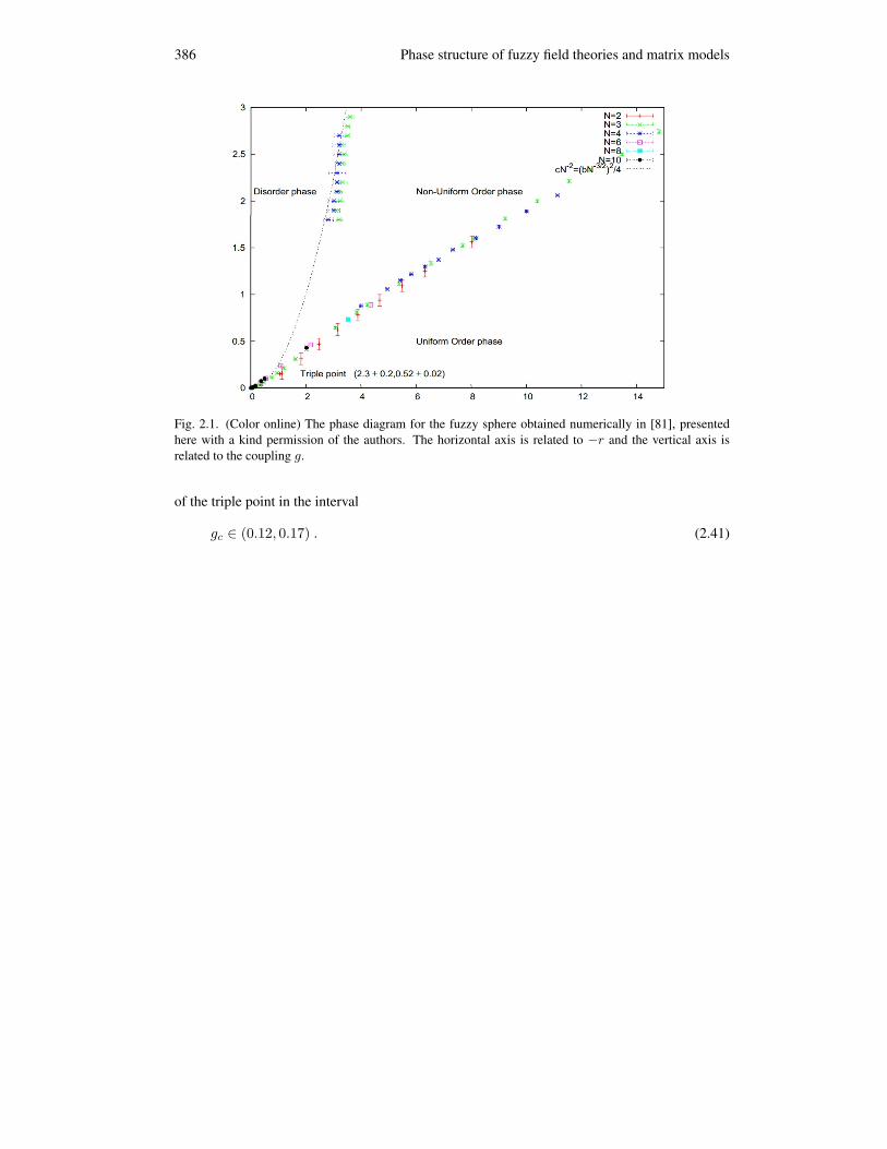
386 Phase structure of fuzzy field theories and matrix models
Fig. 2.1. (Color online) The phase diagram for the fuzzy sphere obtained numerically in [81], presentedhere with a kind permission of the authors. The horizontal axis is related to −r and the vertical axis isrelated to the coupling g.
of the triple point in the interval
gc ∈ (0.12, 0.17) . (2.41)

Matrix models 387
3 Matrix models
This sections reviews matrix models, with the most important notions and techniques. We explainthe properties of ensembles of random matrices and investigate the limit of a large matrix size.We then show computational technique of the saddle point approximation and how it can be usedto calculate the quantities of interest in this limit. In the second part of this section we studymore complicated matrix ensembles characterized by a higher power of a trace of the matrixin the probability distribution and show how to use the saddle point approximation there. Weelaborate on several examples to make the ideas as clear and understandable as possible.
A number of wonderful reviews of matrix model techniques is available. A classic, yeta mathematically minded [33], several other reviews [83, 84, 85, 86] or very readable originalpapers [87, 90]. Some of the techniques are nicely reviewed in [36, 37, 38].
3.1 General aspects of the matrix models
We start with the description of the single trace Hermitian matrix models and the treatment ofthe limit of large matrix size.
3.1.1 Ensembles
As mentioned in the introduction, random matrix theory is given by the ensemble of matrices Mwith the integration measure dM and the probability measure exp−S(M). The expected valueof a function f(M) of the random matrix is then computed as
〈f〉 =1Z
∫dMe−S(M)f(M) . (3.1)
Here, the normalization 1/Z is such that 〈1〉 = 1.The ensemble usually has some symmetry and it is assumed that the integration measure dM ,
as well as the weight S(M) and any reasonable function f(M) are symmetric also.The choice of the matrix ensemble is then dictated by the physical or mathematical setup.
Most usually, matrix M is hermitian, real symmetric or quaternionic self-dual, with SU(N),SO(N) and Sp(2N), or a sub-group, being the symmetry group. Matrix M can be also directlyan unitary, orthogonal or symplectic matrix. In some mathematical applications, such as statisticsor number theory, more complicated matrices, which need not to be square, arise, see e.g. [86].
The most general choice of the probability measure is then dictated by the choice of theensemble and the symmetry group. To be more precise, let M be a square N × N matrix withsymmetry group G, with the action M → gMg−1 with g ∈ G. We then write the measure ase−N2S(M), the factor of N2 makes it explicit that the measure is of the same order as dM andthus contributes. The action S(M) is then finite in the limit of large N . Then, the most generalinvariant measure is given by
S(M) =1N
N∑n=0
gnTr (Mn) , (3.2)
where the factor of 1/N ensures proper large N limit, as the sum of N eigenvalues is of the orderN . Any other invariant function can be re-expressed in terms of the first N traces. The constant

388 Phase structure of fuzzy field theories and matrix models
and the linear terms are usually not considered, since they can be absorbed into redefinition ofM . Also, the M2 term is usually considered separately and we write
S(M) =12r
1N
Tr(M2)
+N∑
n=3
gn1N
Tr (Mn) . (3.3)
This is because of the fact that the n ≥ 3 terms introduce “interactions” into the theory, whichmeans that this renders also some of the higher order correlation functions nontrivial. Theorywith only Tr
(M2)
term can be solved exactly and the extra terms can be considered as a pertur-bation.
We will treat the measure dM explicitly only for the case of N ×N Hermitian matrices. Inthe general case, upon the diagonalization of the matrix, the measure will become
dM = J(λ)dΛdU , (3.4)
where dΛ is the measure on the space of eigenvalues λ of M , dU is the measure of the symmetrygroup G and J(λ) is Jacobian corresponding to the change of variables from Mij to λ and U . Inthe case of Hermitian matrices, G = SU(N) and the integration measure is given by
dM =n∏
i=1
Mii
∏i<j
dReMij dImMij . (3.5)
We can diagonalize the matrix
M = UΛU† , (3.6)
where Λ = diag (λ1, . . . , λN ) is the diagonal matrix of the eigenvalues of M . The integrationmeasure then becomes
dM =
∏i<j
(λi − λj)2
( N∏i=1
dλi
)dU . (3.7)
There are number of ways how to compute the Jacobian, which turned out to be the square of theVandermonde determinant in this case. Thanks to the invariance of the measure, J depends onlyon λ’s, and we can compute it in the vicinity of U = 1. Here
dM = dUΛ + dΛ + ΛdU† = dΛ + ΛdU − dUΛ , (3.8)
where we have used dU† = −dU . This means that
dMij = dλiδij + (λi − λj)dUij , (3.9)
the change of variables is diagonal and the Jacobian is just the product of the factors (λi − λj).

Matrix models 389
Fig. 3.1. Figure shows the double-line notation of a matrix element Mij and the double line notation of aquartic vertex MabMbcMcdMda.
3.1.2 Planar limit as the leading order in the limit of large matrices
One is usually interested in the behavior of the results in the limit of a very large matrix. For thecase of N × N Hermitian matrices this means N → ∞ limit. There are many reasons for this,being mathematical, physical and also practical.
From the mathematical point of view, the quantities like eigenvalue distribution become con-tinuous in the large matrix limit. Also in this limit, certain properties of eigenvalue distributionbecome independent of the exact probability distribution and depend only on the symmetry groupof the ensemble. This notion is called universality and allows to study certain properties on thesimplest ensembles [33].
When random matrices describe a physical system, large matrix limit is the limit of largenumber of constituents. When studying the spectra of large nuclei, this means large number oflevels. In condensed matter this means large number of electrons or other particles of interest.When one uses the random matrix to describe a lattice or to discretize some surface, large Nlimit is the continuum limit. In all these cases the limit is well justified by the physics of theproblem.
When one considers field theory on a fuzzy space, large N limit is the limit of commutativetheory and if the fuzzy structure was introduced to regulate the theory, this removes the regulator.Also, if there is noncommutativity present in the nature, it is very small and this justifies the limitof large N . The subleading contributions then represent the non-commutative correction.
And lastly, the large N limit provides a considerable simplification to the calculations. As wewill see, the diagrams involved in computation of the averages give contributions with differentpowers of N and this power is related to the topology of the diagram. The leading order isgiven by the planar diagrams and this simplifies greatly the resulting combinatorial problem.The subleading corrections can then be computed systematically.
To compute expectation values of invariant functions f(M), one has to compute correlatorsof the form
⟨Tr(Mk)[W (M)]l
⟩. To compute these, we use the Wick’s theorem. One has to sum
over all possible pairing of M ’s in the expectation value, weighted by a propagator MijMkl foreach pairing. Since the contractions are done with the Gaussian, or free, measure, the propagatoris given by the inverse of the quadratic part of (3.3) and is equal to
MijMkl =1
Nrδilδjk . (3.10)
To compute the higher correlators, we use method of fat graphs due to ’t Hooft [34]. Wewill indicate the matrix M in the diagrams by a double line, which represent the double indexstructure of Mij . Since the matrix is in the adjoint representation of SU(N), indexes i and jcan be viewed as in the fundamental and anti-fundamental representation and the lines and thearrows reflect this structure. This is illustrated in the figure 3.1. Vertices are then given by a star

390 Phase structure of fuzzy field theories and matrix models
a) b)
Fig. 3.2. a) shows the planar diagram contribution to the g1 order of the two point function˙MijMklTr
`M4
´¸, b) the nonplanar contribution.
of n double lined legs. Let us illustrate this at the computation of the first order correction to thetwo point function 〈MijMkl〉 of the theory with quartic interaction gTr
(M4).
The relevant diagrams are shown in the figure 3.2. There are two possible kinds of contrac-tions, one planar 3.2a and one non-planar 3.2b. They give respective contributions
planar = Ng1
Nrδiaδjb
1Nr
δblδik1
Nrδddδic =
1N
g
(1r
)3
δikδjl (3.11)
and
non-planar = Ng1
Nrδiaδjb
1Nr
δabδcd1
Nrδdkδcl
=1
N2g
(1r
)3
δijδkl . (3.12)
Following the summation of indexes on delta functions we observe that the overall factor of Ndepends on the number of closed lines in our fat graph. Each line produces, after the summationof all but one of the indexes, factor of δii, which then gives a factor of N when summed over thelast index.
Now comes a crucial observation for a general diagram. Let it have E propagators, or edges,Vn vertices with n legs and h closed loops. The factor for this diagram is then(
1Nr
)E
NhN∏
n=3
(−Ngn)Vn , (3.13)
where V =∑
Vn is the total number of vertices. If we now consider the diagram as a Riemannsurface of genus g, we have the topological relation
2− 2g = h− E + V. (3.14)
So (3.13) can be rewritten as
N2
[(1r
)E∏(−gn)Vn
][1
N2
]g
. (3.15)
We see that the first factor is given by the type of the diagram. The second factor is given by thetopology of the diagram and diagrams of the same type, with higher genus g are all suppressedby a factor of 1/N2g . This also means that the leading order contribution is given by the g = 0,i.e. planar diagrams.

Matrix models 391
To connect the two-point functions (3.11) and (3.12) to this result, we need to realize thatthe two diagrams cannot be realized as Riemann surfaces, since they are not an average of aninvariant function of the form Tr
(Mk). In order to be able to do so, we need to contract the
two external matrices with δikδjl, i.e. to close the loops, and consider them as a new, 2-pointvertex, which brings an extra factor of N . Then, we see that the planar diagram really has N2
dependence, and the non-planar N0.
3.2 Saddle point approximation (for symmetric quartic potential)
This section introduces our main tool to analyze the matrix models, the saddle point approxima-tion.
3.2.1 General aspects of the saddle point method
In this section, we will show how to obtain the eigenvalue distribution of the random matrixwithout explicit computation of any expectation values. We will later show that doing that andcounting the diagrams leads to the same result as computed here.
We absorb the Jacobian in (3.7) into the action and obtain a theory governed by the measure
N2SV (λ) = N2
12r
1N
N∑i=1
λ2i + W (λ)− 2
N2
∑i<j
log |λi − λj |
, (3.16)
where we have denoted the n ≥ 3 part of the measure as
W (λ) =∑
k
gk1N
N∑i=1
λki . (3.17)
In some literature the notation effective in (3.16) is standard, but since we will encounter differentkind of effective quantities two more times in this text, we shall not use this notation. Since wewill need the notation for this object only rarely, we will denote it SV and reserve the termeffective action for something else.
We will assume, that the matrix and the parameters are scaled in such way, that the terms areof order 1 in the large N limit. The key feature will be the fact, that the sums in the expressionare of order N in the large N limit. The Vandermonde term is thus already of order 1 and anyscaling of the matrix ads only a constant term to it, which can be disregarded.
We further introduce scaled quantities
r = rNθr , gk = gkNθk , M = MNθx . (3.18)
The mass terms behaves like N1+θr+2θx and the k-th term of the potential part like N1+θk+kθx .And we want both these to scale as N2, so we obtain conditions
1 = θr + 2θx , 1 = θk + kθx . (3.19)
These do not fix the scaling uniquely and for the simplest choices we get
θr = 0 , θx =12
, θk = 1− k
2(3.20a)
392 Phase structure of fuzzy field theories and matrix models
θr = 1 , θx = 0 , θk = 1 . (3.20b)
We will not denote the scaled quantities by tilde and write expressions like (3.16), but we willkeep in the back of our mind that such form is achievable for example by using the scaling (3.19).
Therefore as N → ∞, the integral in (3.1) will be dominated by the saddle-point configura-tion of the eigenvalues λE
i , which extremizes the action (3.16), or in other words has the largestprobability. The average of an invariant function f(M) is then given, in the large N limit, by
〈f〉 =N∑
i=1
f(λE
i
). (3.21)
We vary the action with respect to λi to obtain
rλEi + W ′(λE
i ) =2N
∑i 6=j
1λE
i − λEj
, (3.22)
for i = 1, 2, . . . , N . This form of the equation will be very useful later, but often we will workwith the eigenvalue distribution. For the solutions of the equation λE
i , it is formally defined as
ρ(λ) =1N
N∑i=1
δ(λ− λEi ) . (3.23)
This function becomes continuous in the large N limit. For a function of the eigenvalues f(λ)we then have in the large N limit
N∑i=1
f(λi)→ N
∫C
dλ ρ(λ)f(λ) , (3.24)
where the integral is over the support of the distribution, which is a bounded interval or a boundedunion of intervals, thanks to the requirement on the scaling of the action S. Using this property,we change (3.22) to
rλ + W ′(λ) = 2P
∫dλ′
ρ(λ′)λ− λ′
. (3.25)
Here, P∫
denotes the principal value of the integral. We introduce a function, called the planarresolvent,
ω0(z) =1N
∑i
1z − λE
i
=∫
dλρ(λ)z − λ
. (3.26)
It is very important to note, that for large |z|, we have ω0 → 1/z thanks to the normalization ofρ.
Computing a square of the resolvent
ω0(z)2 =1
N2
∑i,j
(1
z − λEi
)(1
z − λEj
)=

Matrix models 393
=− 1N
ω′0(z) +2
N2
∑i,j
(1
λEi − λE
i
)1
z − λEj
. (3.27)
We neglect the second term, as it is subdominant in the large-N limit. We then rewrite thisequation using the saddle point condition (3.22) as
ω0(z)2 =(rλE
i + W ′(λEi ))ω0(z) + P (z) , (3.28)
where
P (z) =1N
∑i
rz + W ′(z)− rλEi −W ′(λE
i )z − λE
i
. (3.29)
This is a quadratic equation for the resolvent, which can be solved as
ω0(z) =12
[rz + W ′(z)−
√[rλE
i + W ′(λEi )]2 − 4P (z)
]. (3.30)
The polynomial P is not know yet, but it is much simpler to determine than ω0 directly from(3.25).
Also note, that the resolvent is not well defined on the support of the eigenvalue distribution,which is clear from both the definition (3.26) and the solution (3.30).
In terms of the resolvent function the eigenvalue distribution can be computed using thediscontinuity equation
ρ(λ) = − 12πi
[ω0(λ + iε)− ω0(λ− iε)] , (3.31)
and equation (3.25) becomes an equation for the resolvent
ω0(z + iε)− ω0(z − iε) = −rz −W ′(z) . (3.32)
3.2.2 One cut and multiple cut assumptions
To proceed further, one has to make an assumption about the topology of the support of thedistribution C. Namely on the number of the disjoint intervals on the real axis which form thissupport, which are going to be referred to as cuts.
One cut assumptionIf C is given by the interval [b, a], the equation (3.32) is solved by
ω0(z) =12
∮C
dz′
2πi
rz′ + W ′(z′)z − z′
√(z − a)(z − b)(z′ − a)(z′ − b)
. (3.33)
To see this, we first realize that from (3.30) we must have(rλE
i + W ′(λEi ))2 − 4P (z) = M(z)2(z − a)(z − b) (3.34)

394 Phase structure of fuzzy field theories and matrix models
for some polynomial M(z), given by the condition
M(z) = PolrλE
i + W ′(λEi )√
(z − a)(z − b), (3.35)
where Pol denotes the polynomial part and which is the result of dividing (3.30) and taking thelarge-N limit. It can be deduced also from
M(z) =∮
0
dz′
2πi
r/z′ + W ′(1/z′)1− zz′
1√(1− az′)(1− bz′)
, (3.36)
with contour around z = 0. Once M is known, the ends of the cut are again given by theasymptotics ω0(z)→ 1/z and∮
C
dz′
2πi
rz′ + W ′(z′)√(z′ − a)(z′ − b)
=0 , (3.37a)∮C
dz′
2πi
z′ [rz′ + W ′(z′)]√(z′ − a)(z′ − b)
=2 . (3.37b)
Once M(z) is known, these are equivalent to requiring
Pol ω0(z) = Pol12
[rz + W ′(z)−M(z)
√(z − a)(z − b)
]= 0 . (3.38)
Finally, the distribution is given by
ρ(λ) =1
2πiM(λ)
√(λ− a)(λ− b) =
12π
M(λ)√
(a− λ)(λ− b) . (3.39)
We have assumed that M(z) > 0. If this is not the case, we are clearly running into trouble. Theone cut assumption is not valid and we need to go further.
Knowing the distribution, one can now compute various expectation values of the theory. Forexample the normalized traces of powers of M are given by
1N
⟨Tr(Mk)⟩
=∫C
dλ λkρ(λ). (3.40)
Similarly, the planar free energy is given by
F0 = − 1N2
log(∫
dM e−N2S(M)
)= − 1
N2log e−N2SV [ρ(λ)] = SV [ρ(λ)] . (3.41)
Note that
SV [ρ(λ)] =12r
∫dλ λ2ρ(λ) +
∫dλ W (λ)ρ(λ)−
− 2∫
dλ dλ′ ρ(λ)ρ(λ′) log |λ− λ′| . (3.42)

Matrix models 395
This formula can however be simplified a little into a form more suitable for numerical integrationwe will do later. For this purpose, we introduce a Lagrange multiplier ξ into the action fixing thenormalization of the eigenvalue distribution
SV [ρ(λ)] =12r
∫dλ λ2ρ(λ) +
∫dλ W (λ)ρ(λ)−
− 2∫
dλ dλ′ ρ(λ)ρ(λ′) log |λ− λ′|+ ξ
(∫dλρ(λ)− 1
). (3.43)
Varying this equation with respect to the density we obtain3.1
12rλ2 + W (λ)− 2
∫dλ′ρ(λ′) log |λ− λ′|+ ξ = 0 , (3.44)
which has to hold for any value of λ. The choice is free, we will mostly chose the larges eigen-value such that we do not have to think too much about the absolute value in the logarithm butother choices are possible. Using this, the free energy can be simplified to
F0 =12
[∫dλ
(12rλ2 + W (λ)
)ρ(λ)− ξ
]. (3.45)
Often in the literature the free energy is defined without the free part
F0 = − 1N2
[log(∫
dM e−N2( 12 rλ2+W (λ))
)− log
(∫dM e−N2( 1
2 rλ2))]
. (3.46)
This is equivalent to removing the vacuum bubbles. We will not do it here, as the free energy isgoing to be a tool for determining the most probable solution at given values of parameters. Thisanswer is unaffected by this removal so we choose the simplest possible definition of F .
We should also mention that the resolvent is connected to the moments of the distribution by
zω(z) =1N
∞∑k=0
⟨Tr(Mk)⟩
zk=
∞∑k=0
ck
zk. (3.47)
This is indeed the defining relation for the full resolvent with contributions from diagrams of anytopology. The planar part is then given by the planar diagrams of
⟨Tr(Mk)⟩
, which togetherwith (3.40) gives our original definition of planar resolvent (3.26).
Two and more cutsThe situation gets more complicated when the potential has more than one minimum. If
the minima are deep enough, the gas of particles can split into two or more disjoint parts, eachlocated in one minimum. In the language of the eigenvalue density, the one cut assumption is nolonger valid and we need to assume a more complicated support of the distribution.
We illustrate the approach on the case of two minima of the potential. We will thereforeassume that the support C is given by the union of two intervals [a, b] and [c, d]. Equation (3.30)the becomes
ω0(z) =12
[rz + W ′(z)−M(z)
√(z − a)(z − b)(z − c)(z − d)
](3.48)
3.1The variation of this equation with respect to λ would yield the saddle point equation (3.25).

396 Phase structure of fuzzy field theories and matrix models
and the endpoints of the intervals are given by∮C
dz′
2πi
rz′ + W ′(z′)√(z′ − a)(z′ − b)
=0 , (3.49a)∮C
dz′
2πi
z′ [rz′ + W ′(z′)]√(z′ − a)(z′ − b)
=0 , (3.49b)∮C
dz′
2πi
(z′)2 [rz′ + W ′(z′)]√(z′ − a)(z′ − b)
=2 , (3.49c)
or by
Pol ω0(z) = Pol12
[rz + W ′(z)−M(z)
√(z − a)(z − b)(z − c)(z − d)
]= 0 . (3.50)
Recall that these are given by the 1/z asymptotics of ω0(z). There are too few conditions todetermine the endpoints! In general for s-cut case, there are s + 1 conditions but 2s unknownsto be determined. Here, we have to make some extra assumptions.
The rescue is the free energy (3.41). Note that the solution with the the lowest free energyhas the largest probability and will dominate the large-N limit.
One can show that assuming the free energy of the system to be minimal gives exactly theextra s − 1 conditions that are needed. One introduces the filling fraction xs of the eigenvaluesin the s-th cut as
xs =∫Cs
dλ ρ(λ) ,∑
s
xs = 1, (3.51)
and the variation of the free energy as a function of xs should vanish. This condition has also avery intuitive physical meaning. Recall the problem as a N particle gas of eigenvalues and letsget back to the two cut case. These now sit in two wells. If we try to move one eigenvalue fromone well to the other, this should cost us no energy in the equilibrium case. If we could gainsomething, the fluctuations of the eigenvalues would eventually make this change spontaneously.If we lose energy this process would happen the other way and at the end of the day, we wouldreach balance given by the no-work-done condition.
The force on the i-the eigenvalue is
f(λ) = −rλi + W ′(λi) +2N
∑i 6=j
1λi − λj
= −rλi + W ′(λi) + 2ω0(λi) . (3.52)
If we now fix the eigenvalues and try to move one eigenvalue from one cut to the next one, thework required is∫ b
c
dλ f(λ) = −∫ b
c
dλ M(λ)√
(z − a)(z − b)(z − c)(z − d) . (3.53)
The no-work-done condition then gives∫ c
b
M(z)√
(z − a)(z − b)(z − c)(z − d) = 0. (3.54)
For a multiple cut solution, similar condition is straightforwardly derived and has to hold betweenany two neighboring cuts.

Matrix models 397
3.2.3 The Wigner semicircle distribution
The simplest example is clearly the no potential case W (λ) = 0 and the probability measuregiven by
S(M) =12rTr(M2)
. (3.55)
The first the condition (3.37a) or (3.38) becomes
r
4(a + b) = 0 ⇒ b = −a , (3.56)
which is the expected symmetric distribution for the symmetric potential. The second condition(3.37) or (3.38) then yields
ra2
4= 1 (3.57)
and
a = 2/√
r . (3.58)
Equation (3.36) or (3.35) then yields M(z) = r and we finally obtain
ω0(z) =12
(rz − r
√z2 − 4
r
), (3.59)
and using the discontinuity equation (3.31) or the expression (3.39), we obtain the celebratedWigner semicircle law
ρ(λ) =r
2π
√4r− λ2 , λ2 <
4r
. (3.60)
Note that this distribution is normalized to 1, which is the result of the assumed scaling. To findout this scaling explicitly, we can either look at the general formulas (3.19) or do something alittle different.
We first solve the model without any rescaling. This normalizes ρ(λ) to N , which is thenumber of eigenvalues, rather than to 1. This yields an eigenvalue distribution
ρ(λ) =r
2π
√4N
r− λ2 , λ2 <
4N
r. (3.61)
Again, introducing rescaled quantities
r = rNθr , M = MNθx , (3.62)
this becomes
ρ(λ)N
= N2θx+θr−1 r
2π
√4rN1−θr−2θx − λ2 , λ2 <
4rN1−θr−2θx . (3.63)

398 Phase structure of fuzzy field theories and matrix models
So we see we obtain the same condition
1− θr − 2θx = 0 . (3.64)
for both the radius and the distribution to finite in the large N . And this is clearly equivalent tothe general formula (3.19).
Let us note, that without the scaling, the eigenvalues would spread to the infinity. This meansthat the Vandermonde repulsion would win over the potential and to include the effect of thepotential, we need to enhance it by a corresponding power of N .
On a little different front, with such scaling, the second moment of the distribution is thengiven by
c2 =ra4
16=
1r
(3.65)
and reflects the fact that the distribution is getting narrower as we increase the r. This is on theother hand very intuitive in the gas analogy, where the steeper potential confines the eigenvaluesin a smaller region. The figure 3.3 illustrates the distribution for several values of r.
3.2.4 The quartic potential
We now introduce a simple interaction potential W (λ) = gλ4, which corresponds to the termgTr
(M4)
in the measure and we have
S(M) =12rTr(M2)
+ gTr(M4)
. (3.66)
Positive rAgain, the condition (3.37a) or (3.38) yields
18(a + b)(5a2g − 2abg + 5b2g + 2r) = 0 , (3.67)
which has a clear solution a = −b =√
δ. In terms of this the second condition gives
34δ2g +
14δr = 1 . (3.68)
The radius of the distribution is then given by
δ =16g
(√r2 + 48g − r
). (3.69)
Equation (3.36) or (3.35) then yields
M(z) = 4gz2 + 2gδ + r (3.70)
and we finally obtain
ω0(z) =12
[4gz3 + rz − (4gz2 + 2gδ + r)
√z2 − δ
], (3.71)
Matrix models 399
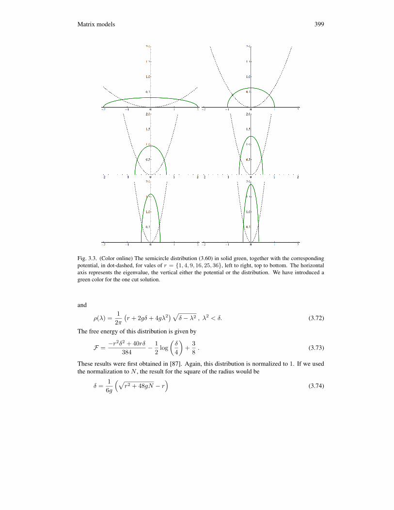
Fig. 3.3. (Color online) The semicircle distribution (3.60) in solid green, together with the correspondingpotential, in dot-dashed, for vales of r = 1, 4, 9, 16, 25, 36, left to right, top to bottom. The horizontalaxis represents the eigenvalue, the vertical either the potential or the distribution. We have introduced agreen color for the one cut solution.
and
ρ(λ) =12π
(r + 2gδ + 4gλ2
)√δ − λ2 , λ2 < δ. (3.72)
The free energy of this distribution is given by
F =−r2δ2 + 40rδ
384− 1
2log(
δ
4
)+
38
. (3.73)
These results were first obtained in [87]. Again, this distribution is normalized to 1. If we usedthe normalization to N , the result for the square of the radius would be
δ =16g
(√r2 + 48gN − r
)(3.74)

400 Phase structure of fuzzy field theories and matrix models
and it is left as an exercise, that this leads to the same scaling as the general formulas (3.19).The moments of the distribution can then be deducted from the 1/z expansion (3.47) or by
explicit integration and are
c2 =14δ3g +
116
δ2r =δ
4+
δ3g
16, (3.75a)
c4 =964
δ4g +132
δ3r =δ2
8+
3δ4g
64. (3.75b)
For positive r, this is the end of the story.
Negative rHowever if we allow for negative r, things change. Potential has then two minima and we
expect a two cut solution to emerge. However not immediately for any value of r, since thepotential price eigenvalues have to pay for being close to the origin has to be large enough toovercome the repulsion of eigenvalues. In other words, the peak that the potential develops at theorigin has to he high enough to split the eigenvalues apart.
There are two ways to treat this situation. First, we can look at the one cut distribution (3.72)and see, that for some value of r, the distribution becomes negative. This indicates that somethingis going wrong and we have to start over. Clearly, the distribution becomes negative at x = 0, sothe condition becomes M(0) = 0 and
r +13
(√r2 + 48g − r
)= 0 ⇒ r = −4
√g . (3.76)
This tells us, where the behavior of the solution should change, but does not tell us what the newsolution is.
Two cut solutionThe second approach is to directly look for this solution. To find it, we look for a symmetric
two cut solution with the support
C =(−√
D + δ,−√
D − δ)∪(√
D − δ,√
D + δ)
. (3.77)
The conditions (3.37),(3.38) become
4Dg + r =0 , (3.78a)
δ2 =1g
(3.78b)
and are trivial to solve. For the solution to be well defined, we must have D − δ > 0, whichyields
r < −4√
g , (3.79)
in agreement with (3.76). The polynomial M(z) becomes simply
M(z) = 4g|z| (3.80)
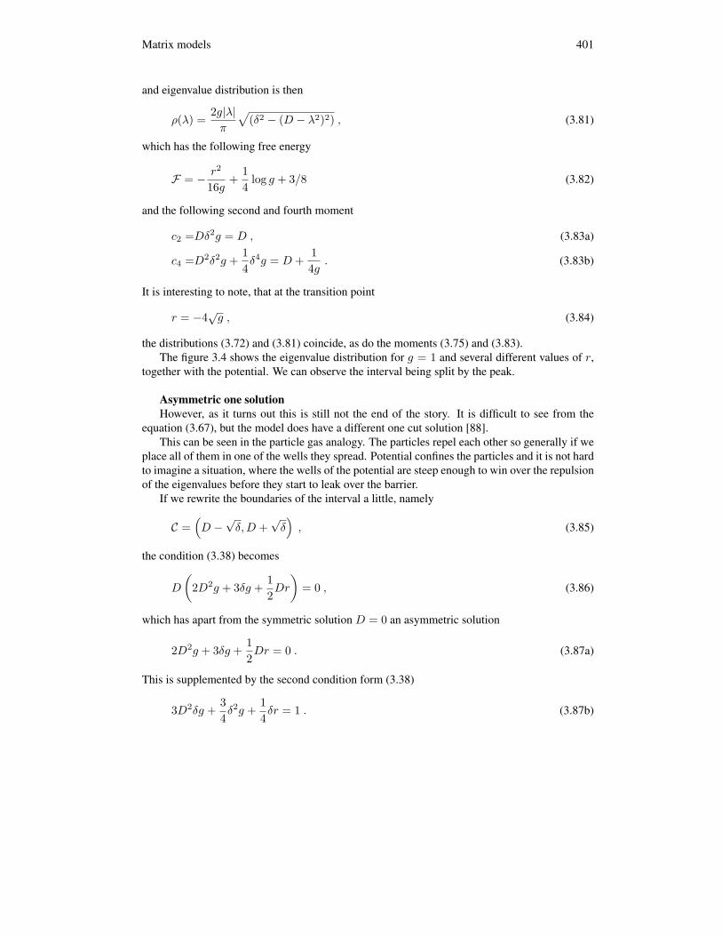
Matrix models 401
and eigenvalue distribution is then
ρ(λ) =2g|λ|
π
√(δ2 − (D − λ2)2) , (3.81)
which has the following free energy
F = − r2
16g+
14
log g + 3/8 (3.82)
and the following second and fourth moment
c2 =Dδ2g = D , (3.83a)
c4 =D2δ2g +14δ4g = D +
14g
. (3.83b)
It is interesting to note, that at the transition point
r = −4√
g , (3.84)
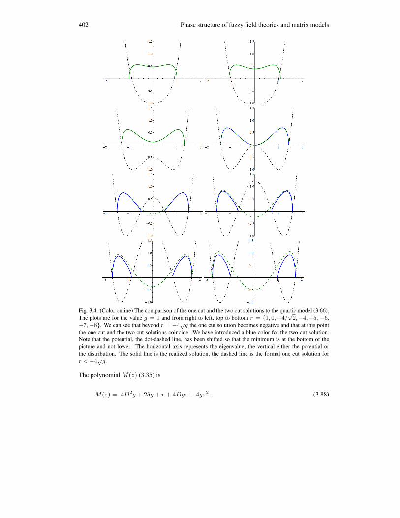
the distributions (3.72) and (3.81) coincide, as do the moments (3.75) and (3.83).The figure 3.4 shows the eigenvalue distribution for g = 1 and several different values of r,
together with the potential. We can observe the interval being split by the peak.
Asymmetric one solutionHowever, as it turns out this is still not the end of the story. It is difficult to see from the
equation (3.67), but the model does have a different one cut solution [88].This can be seen in the particle gas analogy. The particles repel each other so generally if we
place all of them in one of the wells they spread. Potential confines the particles and it is not hardto imagine a situation, where the wells of the potential are steep enough to win over the repulsionof the eigenvalues before they start to leak over the barrier.
If we rewrite the boundaries of the interval a little, namely
C =(D −
√δ, D +
√δ)
, (3.85)
the condition (3.38) becomes
D
(2D2g + 3δg +
12Dr
)= 0 , (3.86)
which has apart from the symmetric solution D = 0 an asymmetric solution
2D2g + 3δg +12Dr = 0 . (3.87a)
This is supplemented by the second condition form (3.38)
3D2δg +34δ2g +
14δr = 1 . (3.87b)
402 Phase structure of fuzzy field theories and matrix models
Fig. 3.4. (Color online) The comparison of the one cut and the two cut solutions to the quartic model (3.66).The plots are for the value g = 1 and from right to left, top to bottom r = 1, 0,−4/
√2,−4,−5, −6,
−7, −8. We can see that beyond r = −4√
g the one cut solution becomes negative and that at this pointthe one cut and the two cut solutions coincide. We have introduced a blue color for the two cut solution.Note that the potential, the dot-dashed line, has been shifted so that the minimum is at the bottom of thepicture and not lower. The horizontal axis represents the eigenvalue, the vertical either the potential orthe distribution. The solid line is the realized solution, the dashed line is the formal one cut solution forr < −4
√g.
The polynomial M(z) (3.35) is
M(z) = 4D2g + 2δg + r + 4Dgz + 4gz2 , (3.88)

Matrix models 403
and the solution of the equations (3.87) is given by
δ =−r −
√−60g + r2
15g, D = ±
√−3r + 2
√−60g + r2
20g(3.89)
and there is plenty to be noticed about it. First, there are two solutions with the same δ andopposite D, which says that the distribution can live in either well of the potential. Second, itexist only for negative r, as δ has to be positive. And since both D and δ have to be real, weobtain r < −2
√15g. Finally, for |r| very large, we get
δ = 0 , D = ±12
√−r
g, (3.90)
which is easily seen to be the location of the minima of the potential. And as expected, in thelimit r → −∞, as the walls of the potential well become very steep, the eigenvalues becomelocalized at its bottom.
And finally, the formula for the distribution itself is
ρ(λ) =12π
(4D2g + 4Dgx + 2δg + r + 4gx2
)√(D +
√δ − x
)(x−D +
√δ)
=
=12π
(4D2g + 4Dgx + 2δg + r + 4gx2
)√δ − (x−D)2 (3.91)
and the free energy of this solution is given by the rather unappealing formula
F =δ
8
[916
g2δ3 + δ2
(58gr +
272
g2D2
)+ δ
(33g2D2 +
152
grD2 +r2
8+
15g
)
+ 15g2D6 + 7grD4 +(
12g +12r2
)D2 + 3r
]+
14rD2 +
12gD4 − 1
2log(
δ
4
)− 1
(3.92)
In the figure 3.5, the asymmetric one cut solution is plotted, together with the two cut solution,for the value of g = 1.
It is interesting to compute the asymmetric eigenvalue density just when it starts to be possi-ble. We plug r = −2
√15g into (3.90) and obtain for the edges of the interval
±(
160g
)1/4
and ± 5(
160g
)1/4
. (3.93)
Note that the interval does not start at 0, but at some depth into the well. This is easily understoodin the particle gas analogy. The particle at the edge of the interval is being repelled by the rest ofthe particles. So there has to be a force acting on it in the opposite direction and thus it cannot sitat the top of the peak at x = 0.
The last question to answer is, which of the two solutions that exist in the region r < −2√
15gis eventually realized. This depends how we look at the model. We can either view the large N

404 Phase structure of fuzzy field theories and matrix models
Fig. 3.5. (Color online) Plot of the asymmetric one cut solution (3.91) to the model (3.66) for the valueg = 1 and for left to right, top to bottom r = −2
√15,−9,−12,−15,−30,−80, together with (a part
of) the potential, shown in dot-dashed. Note that the potential has been shifted so that the minimum is atthe bottom of the picture and not lower. The horizontal axis represents the eigenvalue, tho vertical eitherthe potential or the distribution. We have introduced the red color for the asymmetric one cut solution. Thedashed line is the two cut solution, which is energetically preferred.
limit as a process. Then 1/N2 plays the role of a temperature and the large N limit is the limitof freezing the particles in the well. However if we assume that this process takes some ”time”,in the sense that the fluctuations of the eigenvalues can take one state from another sufficientlymany times, the solution with the lowest free energy (3.41) is realized. Or in other words themore probable solution.
If we on the other hand assume that the system is in the N =∞ state to begin with, thereare no thermal fluctuations and the eigenvalues cannot get from one well into another even if itlowers the free energy. This is a view we are not going to take! First of all because we usuallydo have some limiting process in mind3.2 and because it just leaves room for too many solutions,as for example any two cut solution, once it exists, would be stable.
3.2In our case for example the process of taking the noncommutativity parameter to zero.

Matrix models 405
Fig. 3.6. The phase diagram of the quartic model (3.66). Above the solid line, the eigenvalue distributionis in the one cut phase. Under the solid line, the eigenvalue distribution is in the two cut case. Under thedashed line, an asymmetric one cut phase exists, but is not realized as it has higher free energy.
So we are to determine which of the two solutions, the two cut (3.81) and the asymmetric onecut (3.91) has lower free energy in the region where both exist. Without summoning any explicitformulas for the free energy, it is easy to solve the dispute. In the two cut case, eigenvalues arefurther away from each other, so the energy of the interaction lowers. They are also in region oflower potential, so the potential energy lowers. The free energy is thus lower in the two cut caseand the two cut solution is the preferred one everywhere.
So we got our first phase diagram! It is shown in the figure 3.6 and describes the phasestructure of the quartic model (3.66). The figure 3.7 shows the free energies of the two threesolutions, clearly indicating that the asymmetric one cut solution has always higher free energy.
We got only symmetric solutions as the energetically preferred solutions in this model. Wecan use the notion of freezing the solution to obtain a preferred asymmetric solution in the caseof the symmetric potential (3.66).
We first introduce a symmetry breaking term of the form Tr (M) or Tr(M3)
which lowersone of the wells of the potential. If the term is strong enough, the asymmetric solution living inthis well will become the preferred solution since its free energy will be the lowest. After wetake the large-N limit, we remove the symmetry breaking. This brings the two wells back to thesame level again. However the eigenvalues are now frozen in one well and cannot get to the otherone, obtaining an asymmetric solution.
We will not employ this strategy though. The matrix model we will need to study as adescription of the fuzzy field theory will not allow to remove the symmetry breaking term, so wewill have to study the asymmetric models completely. But before that, let us summarize what wehave learned in this section.
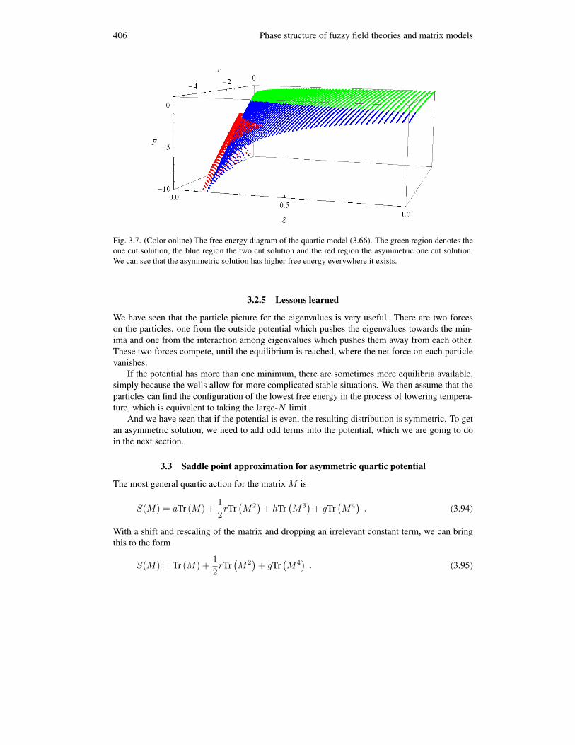
406 Phase structure of fuzzy field theories and matrix models
Fig. 3.7. (Color online) The free energy diagram of the quartic model (3.66). The green region denotes theone cut solution, the blue region the two cut solution and the red region the asymmetric one cut solution.We can see that the asymmetric solution has higher free energy everywhere it exists.
3.2.5 Lessons learned
We have seen that the particle picture for the eigenvalues is very useful. There are two forceson the particles, one from the outside potential which pushes the eigenvalues towards the min-ima and one from the interaction among eigenvalues which pushes them away from each other.These two forces compete, until the equilibrium is reached, where the net force on each particlevanishes.
If the potential has more than one minimum, there are sometimes more equilibria available,simply because the wells allow for more complicated stable situations. We then assume that theparticles can find the configuration of the lowest free energy in the process of lowering tempera-ture, which is equivalent to taking the large-N limit.
And we have seen that if the potential is even, the resulting distribution is symmetric. To getan asymmetric solution, we need to add odd terms into the potential, which we are going to doin the next section.
3.3 Saddle point approximation for asymmetric quartic potential
The most general quartic action for the matrix M is
S(M) = aTr (M) +12rTr(M2)
+ hTr(M3)
+ gTr(M4)
. (3.94)
With a shift and rescaling of the matrix and dropping an irrelevant constant term, we can bringthis to the form
S(M) = Tr (M) +12rTr(M2)
+ gTr(M4)
. (3.95)

Matrix models 407
Such ensemble can be treated by the saddle point approximation in the same way we treated thesymmetric case in the section 3.2.
One cut solutionsFirst, let us consider the one cut solution of this problem. We will discuss the two cut solution
afterward. We have already encounter an ansatz for the general one cut support (3.85)
C = (D −√
δ, D +√
δ) . (3.96)
(3.38) now leads to equations
12
+ 2D3g + 3Dδg +12Dr =0 , (3.97a)
3D2δg +34δ2g +
14δr =1 , (3.97b)
which are slightly more complicated than (3.87). We invite the reader to show, that in the freecase these equations give rise a distribution, which is the original semicircle shifted by 1/r to theleft, which is exactly what we would expect.
The polynomial M(z) (3.35) is the same as (3.88), since it depends only on the form of thecut
M(z) = 4D2g + 2δg + r + 4Dgz + 4gz2 . (3.98)
For a general coupling, because of to the extra term 1/2, the equations are not solvable any-more, as solving (3.97a) for δ turns (3.97b) into the equation of sixth order in D. The momentsof the distribution are given in terms of the solution of these equations by
c1 =3D3δg +32Dδ2g +
14Dδr , (3.99a)
c2 =3D4δg + 3D2δ2g +14δ3g +
14D2δr +
116
δ2r , (3.99b)
c3 =3D5δg +214
D3δ2g +98Dδ3g +
14D3δr +
316
Dδ2r , (3.99c)
c4 =3D6δg +334
D4δ2g +278
D2δ3g +964
δ4g +14D4δr +
38D2δ2r +
132
δ3r . (3.99d)
Every one cut solution of this model is an asymmetric one. However, we are going to distin-guish two kinds of one cut solutions, which are rather different. We are going to them almost-symmetric solution and the asymmetric solution.
As suggested by the name, the almost-symmetric solution is not going to be too differentfrom the symmetric solution (3.72). We will define it by the condition that the extremum of thepolynomial M(z) is within the supporting interval. This means that the eigenvalue distributionwill have two peaks, even though not of the same height.
The asymmetric solution will have this extremum outside of the supporting interval. Thismeans that the eigenvalue distribution will have only one peak and all the eigenvalues will belocated in one well only.

408 Phase structure of fuzzy field theories and matrix models
The extremum of M given by (3.98) occurs at z = −D/2, so in terms of the solution of(3.97), the solution is asymmetric if
32D +
√δ < 0 . (3.100)
To find the phase transition, we need to look for the moment when the asymmetric solution doesnot exists, i.e. when the distribution becomes negative. Since the extremum of the potential isoutside the interval, this will happen at the edge of the interval and we get the condition for theboundary of existence of the asymmetric solution
M(D +√
δ) = 12D2g + 12D√
δg + 6δg + r = 0 . (3.101)
For the almost-symmetric solution, the distribution becomes negative at the minimum of thepotential, so the boundary is given by
M(−D/2) = 3D2g + 2δg + r = 0 . (3.102)
These two equations, together with the conditions (3.97) determine the two boundary lines of theregions, where the two solutions exist. They cannot be solved analytically, but after some algebraD and δ can be removed for the almost symmetric case to give a condition just in terms of r andg
45√
g −√
15[4r +
√−80g + 9r2
]√−2r +
√−80g + 9r2 = 0 , (3.103)
This condition can now be solved either numerically or perturbatively.When doing the perturbative calculation for either case, we introduce a factor of ε in front
of the linear term, see where the ε propagates into (3.103) and look for the solution as a powerseries in ε. The result is
r(g) =332
+2343
8388608g+
12332768
√g− 4√
g (3.104)
for the almost symmetric solution and
r(g) =− 2√
15√
g +151/4g1/4
√2
+112
+199
5184√
2151/4g1/4+
73362208
√15√
g+
+49807
5971968√
2153/4g3/4+
243111337408g
+244091717
1393140695040√
2151/4g5/4(3.105)
for the asymmetric solution. These two lines are shown in the numerical phase diagram of thetheory in the figure 3.8. Note that they intersect and beyond this intersection there is no truedistinction between the two solutions. We will see this better once we plot the solutions a littlelater. In the empty region, only a two cut solution exists.
To obtain this phase diagram of the one cut part of the problem numerically, we have cho-sen particular values of r and g, solve the equations (3.97) with these particular values. Fromthe numerical point of view, it is rather challenging to navigate one’s way around a slew of

Matrix models 409
Fig. 3.8. (Color online) The numerical phase diagram of the asymmetric quartic model (3.95). The redregion denotes the asymmetric one cut solution and the red line the perturbative boundary line (3.105). Thegreen region denotes the almost symmetric one cut solution and the green line the perturbative boundaryline (3.104). Note the difference in the g axis.
solutions. For example figure 3.9 shows all the numerical solution one obtains for the valuesr = −12, g = 1/2. Once drawn, it is clear which solution is the correct one. It is however usefulto be able to determine the correct solution just from the values of D and δ. Once all the imagi-nary results and negative δ’s are thrown away, it is the solution with D closest to the minimumof the potential.
We have exhausted the discussion of the one cut solution and will proceed to the descriptionof the two cut solution. It has to be the solution of the model in the blank region in the figure 3.8,but as we will see it exists also outside this area.
Two cut solutionThe ansatz for a general two cut solution is
C = (D1 − δ1, D1 + δ1) ∪ (D2 − δ2, D2 + δ2) . (3.106)
The three conditions we get from (3.38), recall that it is the condition ω(z) ∼ 1/z for large z, arethen
2D21g + 2D1D2g + 2D2
2g + δ21g + δ2
2g +12r = 0 , (3.107a)
12− 2D2
1D2g − 2D1D22g + 2D1δ
21g + 2D2δ
22g = 0 , (3.107b)
2D21δ
21g −D1D2δ
21g −D2
2δ21g +
14δ41g −D2
1δ22g−

410 Phase structure of fuzzy field theories and matrix models
Fig. 3.9. All the real solutions to equations (3.97) obtained numerically at r = −12, g = 1/2. The dot-dashed line is the potential, the dashed lines are the negative solutions and are not well defined. The solidsolutions are well defined but the solution in the right well has higher free energy.
−D1D2δ22g + 2D2
2δ22g − 1
2δ21δ2
2g +14δ42g = 1 . (3.107c)
The polynomial M(z) is given by
M(z) = 4 (D1 + D2 + g) (3.108)
and the distribution becomes
ρ(λ) =2|D1 + D2 + g|
π
√(δ2
2 − (D1 − λ)2) (δ22 − (D2 − λ)2) , (3.109)
The moments of the distribution are given by
c1 =2D31δ
21g −D2
1D2δ21g −D1D
22δ
21g + D1δ
41g −D2
1D2δ22g
−D1D22δ
22g + 2D3
2δ22g −D1δ
21δ2
2g −D2δ21δ2
2g + D2δ42g , (3.110a)
c2 =2D41δ
21g −D3
1D2δ21g −D2
1D22δ
21g +
94D2
1δ41g − 1
4D1D2δ
41g
− 14D2
2δ41g +
18δ61g)−D2
1D22δ
22g −D1D
32δ
22g + 2D4
2δ22g
−D21δ
21δ2
2g − 32D1D2δ
21δ2
2g −D22δ
21δ2
2g − 18δ41δ2
2g
− 14D2
1δ42g − 1
4D1D2δ
42g +
94D2
2δ42g − 1
8δ21δ4
2g +18δ62g) , (3.110b)
c3 =2D51δ
21g −D4
1D2δ21g −D3
1D22δ
21g + 4D3
1δ41g − 3
4D2
1D2δ41g
− 34D1D
22δ
41g +
34D1δ
61g −D2
1D32δ
22g −D1D
42δ
22g + 2D5
2δ22g

Matrix models 411
−D31δ
21δ2
2g − 32D2
1D2δ21δ2
2g − 32D1D
22δ
21δ2
2g −D32δ
21δ2
2g − 12D1δ
41δ2
2g
− 14D2δ
41δ2
2g − 34D2
1D2δ42g − 3
4D1D
22δ
42g + 4D3
2δ42g − 1
4D1δ
21δ4
2g
− 12D2δ
21δ4
2g +34D2δ
62g , (3.110c)
c4 =2D61δ
21g −D5
1D2δ21g −D4
1D22δ
21g +
254
D41δ
41g − 3
2D3
1D2δ41g
− 32D2
1D22δ
41g +
52D2
1δ61g − 1
8D1D2δ
61g − 1
8D2
2δ61g +
564
δ81g
−D21D
42δ
22g −D1D
52δ
22g + 2D6
2δ22g −D4
1δ21δ2
2g − 32D3
1D2δ21δ2
2g
− 32D2
1D22δ
21δ2
2g − 32D1D
32δ
21δ2
2g −D42δ
21δ2
2g − 98D2
1δ41δ2
2g − 78D1D2δ
41δ2
2g
− 14D2
2δ41δ2
2g − 116
δ61δ2
2g − 32D2
1D22δ
42g − 3
2D1D
32δ
42g +
254
D42δ
42g
− 14D2
1δ21δ4
2g − 78D1D2δ
21δ4
2g − 98D2
2δ21δ4
2g − 132
δ41δ4
2g − 18D2
1δ62g
− 18D1D2δ
62g +
52D2
2δ62g − 1
16δ21δ6
2g +564
δ82g . (3.110d)
Finally, the condition for the minimal free energy (3.54) for the asymmetric two cut solution(3.109) becomes
0 =(− 4D5
1 + 12D41D2 − 8D3
1D22 − 8D2
1D32 + 12D1D
42 − 4D5
2 − 10D31δ
21
+ 22D21D2δ
21 − 14D1D
22δ
21 + 2D3
2δ21 + 14D1δ
41 + 2D2δ
41 − 8D3
1δ1δ2
+ 8D21D2δ1δ2 + 8D1D
22δ1δ2 − 8D3
2δ1δ2 − 28D1δ31δ2 − 4D2δ
31δ2 + 2D3
1δ22
− 14D21D2δ
22 + 22D1D
22δ
22 − 10D3
2δ22 + 16D1δ
21δ2
2 + 16D2δ21δ2
2 − 4D1δ1δ32
− 28D2δ1δ32 + 2D1δ
42 + 14D2δ
42
)E
[(D1 −D2)2 − (δ1 + δ2)2
(D1 −D2)2 − (δ1 − δ2)2
]+
+(6D5
1 − 12D31D
22 + 6D1D
42 + 6D4
1δ1 − 12D21D
22δ1 + 6D4
2δ1 + 29D31δ
21
− 12D21D2δ
21 + 15D1D
22δ
21 + 16D3
2δ21 + 29D2
1δ31 + 20D1D2δ
31 −D2
2δ31
+ D1δ41 − 4D2δ
41 + δ5
1 + 8D31δ1δ2 − 8D2
1D2δ1δ2 − 8D1D22δ1δ2 + 8D3
2δ1δ2
+ 28D1δ31δ2 + 4D2δ
31δ2 + 15D3
1δ22 + 36D2
1D2δ22 − 3D1D
22δ
22 −D2
1δ1δ22
+ 20D1D2δ1δ22 + 29D2
2δ1δ22 − 30D1δ
21δ2
2 − 28D2δ21δ2
2 − 2δ31δ2
2
+ 4D1δ1δ32 + 28D2δ1δ
32 − 3D1δ
42 + δ1δ
42
)K
[(D1 −D2)2 − (δ1 + δ2)2
(D1 −D2)2 − (δ1 − δ2)2
]+
+(− 12D4
1δ1 + 24D21D
22δ1 − 12D4
2δ1 − 58D21δ
31 − 40D1D2δ
31
+ 2D22δ
31 − 2δ5
1 + 2D21δ1δ
22 − 40D1D2δ1δ
22 − 58D2
2δ1δ22

412 Phase structure of fuzzy field theories and matrix models
Fig. 3.10. (Color online) The phase diagram of the asymmetric model (3.95) including the two cut phase.The color code is as before, green for the almost symmetric one cut, red for the asymmetric one cut andblue for the two cut solution. Note that the dots of the two cut solution have been shifted slightly to theright to the right not to overlap with the red dots. See the text for details.
+ 4δ31δ2
2 − 2δ1δ42
)Π[D1 −D2 − δ1 − δ2
D1 −D2 + δ1 − δ2,(D1 −D2)2 − (δ1 + δ2)2
(D1 −D2)2 − (δ1 − δ2)2
](3.110e)
where K is the complete elliptic integral of the first kind, E is the complete elliptic integral ofthe second kind and Π is the complete elliptic integral of the third kind.
The mission is now straightforward. Solve equations (3.110) and obtain the parametersD1,2, δ1,2. However these equations are not only beyond any chance to solve analytically, butalso their numerical treatment is extremely complicated. Available computer programs cannotbe used, since the equations are very sensitive to the starting point used as the first trial in thenumerical computation and there is very little we can do systematically here.
We have thus programed our own algorithm to deal with the equations (3.110) described inthe appendix A. It is almost surely far from being optimal both in precision and speed, but itgives results sufficiently fast and precise for our purposes.
Using this algorithm, we obtain the phase diagram shown in the figure 3.10. The first thingto notice is no overlap of the region of the symmetric one cut and the two cut solutions, i.e. greenand the blue regions, as is expected. And there is an overlap between the asymmetric one cut andthe two cut, i.e. the blue and the red regions, as expected. In this region, both the asymmetricone cut and the two cut solutions exists. And we identify a region, where only an asymmetricone cut solution exists. We see, that our algorithm did miss several points along the boundaryof this area. The numerics becomes very sensitive and it is extremely challenging to pin downthe boundary precisely. Fortunately, we will not need the exact location of the boundary for ourpurposes.

Matrix models 413
Fig. 3.11. (Color online) Plots of the eigenvalue distribution of the asymmetric quartic model (3.95). Theplots are for the value g = 0.1 and from right to left, top to bottom r = 0,−0.91,−1.19, −1.47, −1.68,−2.66, −5.04,−5.32. In dashed are shown the solutions which either do not exist or have higher freeenergy. We can see that beyond some value of r, the asymmetric one cut solution becomes the profferedone, thanks to the large enough difference between the two minima. Note that the potential has beenshifted vertically and rescaled so that it fits into the figure, so the differences between the extrema were notpreserved. But it has been not shifted horizontally, so the position of the extrema of the potential have beenpreserved.
For a better idea what happens there, we give a series of plots of the distributions in the figure3.11.
As we lower the value of r, the two wells of the potential become too deep for a solutionextending over both of the wells to exists and we obtain a two cut solution. As we go lower withr, the walls of the left well become steep enough to confine all the eigenvalues in the left well,which has a lower potential.3.3 However, such situation has a large free energy. But as we go
3.3There might be a solution living also in the right well, but it always has a higher free energy.

414 Phase structure of fuzzy field theories and matrix models
Fig. 3.12. (Color online) The free energy diagram of the asymmetric model (3.95). The free energy of thetwo cut solution is shown as a filled area to emphasize its location in the diagram. See the text for details.
even further lower with the value of r, the difference between the right and the left well becomesso large, that the energy loss for the eigenvalue when moving into from the right to the left wellis high enough to pay for the energy gain in the interaction energy. The two cut solution with thelowest free energy is the asymmetric one cut solution living in the left well.
This is shown in the free energy diagram in the figure 3.12. We can see how the free energyof the two cut solution interpolates between the energies of the two one cut solutions.
Let us note, that to our best knowledge the asymmetric quartic model has not been analyzedin this detail in the literature.
3.4 Saddle point approximation for multitrace matrix models
Up to now, we have considered only matrix models with simple polynomial action (3.16). Wewould now like to generalize our treatment for more complicated models. Recalling the formulafor the moments of the distribution (3.40) we see that (3.2) is simply
S(M) =∑
gncn , (3.111)
a linear expression in moments. A natural way to generalize such action is to include nonlinearterms into the action and consider a general action
S(M) = f(c1, c2, . . .) +12rTr(M2)
+ gTr(M4)
, (3.112)
where we have considered an addition of a new term to the original quartic action. We will referto this kind of models as multitrace models, opposing to the single trace models (3.2). Suchmodels arise when the matrix M is coupled to some external matrix A via some interactionterm Tr (MA) or Tr (MAMA) [89]. Such terms are not invariant under M → UMU† and theangular integral will not be trivial anymore. We will see an explicit example of this for the caseof the scalar field on the fuzzy sphere in the sections 4.1 and 4.2.

Matrix models 415
The integration will introduce a multitrace term of the form (3.112), with the function f givenby the form of the interaction and the eigenvalues of the matrix A [90]. We will not consider anygeneral cases here and after a swift description of the saddle point approximation we will workour way through several examples slowly building apparatus towards the matrix models whichdescribe the scalar field theory on the fuzzy spaces.
3.4.1 General aspects of multitrace matrix models
To derive the saddle point equation for the action (3.112), we need to realize that the variation of
cnm =
∑j
λmj
n
(3.113)
with respect to the i-th eigenvalue is
d(cnm) = n
∑j
λmj
n−1
∂
∂λi
∑j
λmj
dλi = ncn−1m mλm−1
i dλi (3.114)
and we get
∂cnm
∂λi= ncn−1
m mλm−1i . (3.115)
If we have more than one moment coupled to each other, we straightforwardly get
∂cm1cm2
∂λi= cm1m2λ
m2i + cm2m1λ
m1i (3.116)
and similarly for more moments coupled in a more complicated way. This way we obtain thesaddle point equation of a general form∑
n
∂f
∂cnnλn−1
i + rλi + 4gλi =2N
∑i 6=j
1λi − λj
. (3.117)
This means, that multitrace terms will introduce terms into saddle point equation, whichinclude the moments of the distribution multiplied by λi. If we view the saddle point equationas the equilibrium condition for the gas of particles, these terms generate a force on the i-theigenvalue which depends on the position of other eigenvalues. This means that they introducefurther selfinteraction among the eigenvalues. However this is not a standard pair interactionbetween two particles. Multitrace terms rather couple the eigenvalue to an overall distribution ofall the eigenvalues.
The approach we will use is based on rewriting the saddle point equation as an equation of aneffective matrix model, which has only single traces in the potential. This is the second time wehave encountered the word effective. There will be one more setting where we will use the wordeffective. To distinguish this effectivnes from the future one, we will always refer to this as an

416 Phase structure of fuzzy field theories and matrix models
effective single trace model, action of the effective single trace model, moments of the effectivesingle trace model, etc.
The form of the saddle point equation will thus be∑n
gn,effλn−1i =
2N
∑i 6=j
1λi − λj
. (3.118)
This way, appearance of cnm will be seen as a correction to the coupling constant gm → gm,eff .
We then compute the eigenvalue distribution of this effective single trace model as if these pa-rameters were constant. After that the moments of the effective distribution will be functionsof the effective couplings and thus of the moments themselves. Equations for the moments like(3.75) for example will thus turn into a set of selfconsistency conditions. Simply because
cn =∫
dλ λnρ(λ, gn,eff ) =∫
dλ λnρ(λ, c1, c2, . . .) (3.119)
the eigenvalue distribution to be used to compute the moments is a function of moments them-selves. The solution will be valid however only in the large N limit, as what we effectively do iswe rewrite
Tr (Mn)m =⟨
Tr (Mn)m−1⟩
Tr (Mn) (3.120)
which uses the factorization property valid only in the large N limit.Technically, there is really not much more to it. It is good to keep in mind the picture, where
the eigenvalues create an outside force among themselves that acts on them. With that in mind,we shall proceed to some, gradually more complicated, examples.
We will first study matrix models which have the standard quartic potential in the actionaccompanied by a multitrace part that contains even moments of the distribution
S(M) = f(c2, c4, . . .) +12rTr(M2)
+ gTr(M4)
. (3.121)
We thus expect the resulting distributions to be symmetric. Later, we will get to some simpleexamples of models involving also asymmetric moments in the multitrace.
3.4.2 Second moment multitrace models
Let us start with a very simple model which we will use to illustrate the method outlined in theprevious part. As the name of the section suggests, we will deal with models involving only thesecond moment in the multitrace.
The most simple modelLet the multitrace part be given just by the square of the second moment
S(M) = c22 +
12rTr(M2)
+ gTr(M4)
. (3.122)

Matrix models 417
According to (3.115), the saddle point equation for this model is given by
2c2λi + rλi + 4gλ2i =
2N
∑i 6=j
1λi − λj
(3.123)
and can be rewritten as
[r + 2c2]λi + 4gλ2i =
2N
∑i 6=j
1λi − λj
. (3.124)
If we now denote
reff = r + 2c2 , (3.125)
this corresponds to the well-known and by now very familiar quartic model. The one cut solution(3.72), together with the expression for the second moment (3.75a) leads to a rather unappealingunsolvable equation. However, at the phase transition, things simplify. First of all at the phasetransition
reff = r + 2c2 = −4√
g (3.126)
and as we have seen at the phase transition the second moment of the distribution is independentof reff and is equal to 1/
√g. A little surprisingly we obtain a phase transition of the line
r = −4√
g − 2√
g. (3.127)
We are tempted to conclude that for any point in the parameter space under this line, we obtain atwo cut solution but this is something not to be taken for granted. We will investigate this further.
The conditions for the two cut solution (3.78) are much simpler. reff = r + 2c2 with (3.83a)yields
c2 =−r
2 + 4g. (3.128)
This is a well-defined positive number everywhere under (3.127) and thus the solution existsin the whole region. To understand better what is happening, let us investigate how the phasediagram of the effective single trace model and the multitrace model are connected.
The strategy is as follows. We take a point in the phase diagram of the effective single tracemodel (reff , geff ) for some particular values of the parameters. The moments of the effectivedistribution as well as its free energy are then known. We then invert the relation (3.125) toobtain
r = reff − 2c2 . (3.129)
This way, we obtain a point (r, g) in the phase diagram of the original model. We then repeat thisprocedure for different values of the effective parameters, obtaining a deformation of the phasediagram of the effective single trace model.
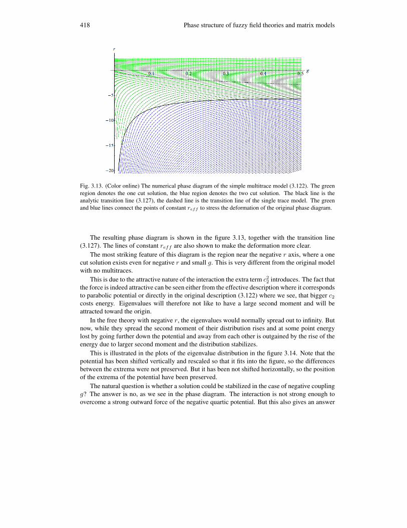
418 Phase structure of fuzzy field theories and matrix models
Fig. 3.13. (Color online) The numerical phase diagram of the simple multitrace model (3.122). The greenregion denotes the one cut solution, the blue region denotes the two cut solution. The black line is theanalytic transition line (3.127), the dashed line is the transition line of the single trace model. The greenand blue lines connect the points of constant reff to stress the deformation of the original phase diagram.
The resulting phase diagram is shown in the figure 3.13, together with the transition line(3.127). The lines of constant reff are also shown to make the deformation more clear.
The most striking feature of this diagram is the region near the negative r axis, where a onecut solution exists even for negative r and small g. This is very different from the original modelwith no multitraces.
This is due to the attractive nature of the interaction the extra term c22 introduces. The fact that
the force is indeed attractive can be seen either from the effective description where it correspondsto parabolic potential or directly in the original description (3.122) where we see, that bigger c2
costs energy. Eigenvalues will therefore not like to have a large second moment and will beattracted toward the origin.
In the free theory with negative r, the eigenvalues would normally spread out to infinity. Butnow, while they spread the second moment of their distribution rises and at some point energylost by going further down the potential and away from each other is outgained by the rise of theenergy due to larger second moment and the distribution stabilizes.
This is illustrated in the plots of the eigenvalue distribution in the figure 3.14. Note that thepotential has been shifted vertically and rescaled so that it fits into the figure, so the differencesbetween the extrema were not preserved. But it has been not shifted horizontally, so the positionof the extrema of the potential have been preserved.
The natural question is whether a solution could be stabilized in the case of negative couplingg? The answer is no, as we see in the phase diagram. The interaction is not strong enough toovercome a strong outward force of the negative quartic potential. But this also gives an answer
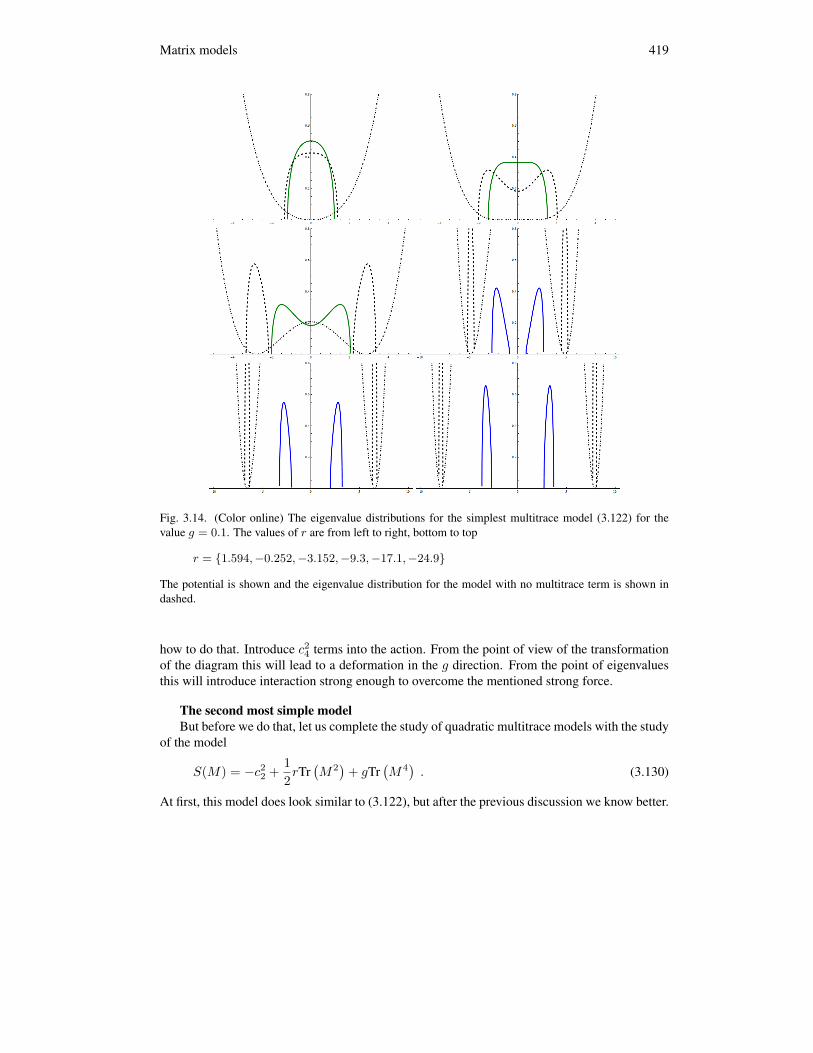
Matrix models 419
Fig. 3.14. (Color online) The eigenvalue distributions for the simplest multitrace model (3.122) for thevalue g = 0.1. The values of r are from left to right, bottom to top
r = 1.594,−0.252,−3.152,−9.3,−17.1,−24.9
The potential is shown and the eigenvalue distribution for the model with no multitrace term is shown indashed.
how to do that. Introduce c24 terms into the action. From the point of view of the transformation
of the diagram this will lead to a deformation in the g direction. From the point of eigenvaluesthis will introduce interaction strong enough to overcome the mentioned strong force.
The second most simple modelBut before we do that, let us complete the study of quadratic multitrace models with the study
of the model
S(M) = −c22 +
12rTr(M2)
+ gTr(M4)
. (3.130)
At first, this model does look similar to (3.122), but after the previous discussion we know better.

420 Phase structure of fuzzy field theories and matrix models
Fig. 3.15. (Color online) The numerical phase diagram of the multitrace model (3.130). The green regiondenotes the one cut solution, the blue region denotes the two cut solution. The black line is the analytictransition line (3.131), the dashed line is the transition line of the single trace model and the horizontal linedenotes the g = 1/2.
The force introduced pushes the eigenvalues outward, as having a high second moment lowersthe energy. The algebra is similar to the previous case and we obtain the phase transition line
r = −4√
g +2√
g(3.131)
and for the second moment of the two cut solution
c2 =−r
4g − 2. (3.132)
This formula already suggests some strange behavior. For r < 0, this expression is positive onlyfor g > 1/2. The system does not have a two cut solution for r < 0, g < 1/2! But it has areasonable two cut solution even for r > 0 if g < 1/2!
This can again be understood in the particle gas picture. The multitrace term introduces arepulsive force among the eigenvalues. They like to have a large second moment and as long asthe potential well is not too steep (which means g small enough) they will start to split. Onlywhen they get far enough from the origin, the potential becomes steep enough to provide enoughforce to tame the repulsion. And as we will see for small r and g, not even that.
And the phase diagram in the figure 3.15 confirms this. Moreover we see that there is a smallregion in the r > 0, g > 0 part of the diagram where no solution exists. And it is not clearwhether there is a two cut solution in the whole area g < 1/2 above and g > 1/2 below theline (3.131). To resolve this issue, we consider the transformation of the line reff = −x
√g for

Matrix models 421
Fig. 3.16. (Color online) The numerical free energy diagram of the multitrace model (3.130). Again, thegreen region denotes the one cut solution, the blue region denotes the two cut solution. See the text fordetailed discussion.
x > 4. This line is transformed into the line
r(g) = x
(−√g +
12√
g
). (3.133)
Therefore, the whole region r > 0, g < 1/2 is covered by some x as is the whole regionr < 0, g > 1/2.
Another question is what happens in the region of overlap between the one cut and the twocut solutions. The answer is in the free energy diagram in the figure 3.16.
The free energy diagram shows what has happened. The part close to the negative r axis hasbeen folded upwards under the part close to the positive r axis. Since the free energy of thispart is lower, the preferred solution is this ”folded” one. So apart from the usual matrix phasetransition at the line (3.131), the model exhibits a new, ”multitrace” phase transition at the lineg = 1/2, r > 0, where the usual one cut solution changes into the ”folded” two cut solution.This phase transition is of the first order, as the free energy is discontinuous.
The last unanswered question is the region where no solution is available close to the origin.To find its boundary, we again consider the transformation of lines reff = −x
√g, but now for
x < 4. After some algebra we find out that such lines transform to
r(g) = −x√
g +72x + x3 + 48
√48 + x2 + x2
√48 + x2
432√
g. (3.134)
The boundary is then given by the envelope of these curves for all values of x < 4. To find thisenvelope, we consider two curves for x and x + dx and find their intersection, which gives onepoint of the enveloping curve. We solve this equation for g and plug into the formula for r. Atthe end of the day, we find the boundary of existence of the one cut solution do be
r(g) =1
108√
2g3/2
( (±1± 24g ∓ 180g2
)√−12 + 1
g + 36g
+(1 + 6g)2√
12 + 1g + 36g
)− g < 1
6+ 1
6 < g < 12
.
(3.135)

422 Phase structure of fuzzy field theories and matrix models
Fig. 3.17. (Color online) The phase diagrams of model (3.136). The green dots denote the existence of theone cut solution, blue of the two cut solution and red of the asymmetric one cut solution.
This line nicely fits into the diagram 3.15, but is not shown to keep the figure clear. The fact thatwe have been able to find this line explicitly is due to a simple form of the multitrace term. Later,for more complicated models we will not be able to do so and the line could be found using thesame method numerically, which we will however not do.
A general c22 model
Similar model has been studied before. Namely the model with F (c2) = hc22 and a fixed
r = −1 in [91], i.e. the model given by the action
S(M) = −12
Tr(M2)
+ hTr(M2)2
+ gTr(M4)
. (3.136)
The phase structure in the (g, h) plane was then considered. It is very easy to analyze thisstructure using the outlined numerical approach.
The figure 3.17 shows the phase diagram of such model. There are three regions in the phasediagram, the green region where only the one cut solution exists, the blue region where only thetwo cut solution exists and the red region, where both the asymmetric one cut solution and thetwo cut solution exist. The three regions are separated by two parabolas, which are not difficultto compute. We take reff = −1 + 4hc2 and reff = −4
√g or reff = −2
√15g for the upper or
the lower boundary respectively. This then yields the two boundary lines
h(g) =14
(√
g − 4g) , (3.137)
h(g) =382
(√15√
g − 30g)
. (3.138)
As we can see, both these expression precisely fit into the diagram 3.17. The green region extendsall the way up for positive h. But since for the second moment we obtain
c2 =1
4(g + h), (3.139)

Matrix models 423
if h < −g the solution is not well defined and does not exist. Which is also seen in the diagram,as there is no solution under the h = −g line.
Note that the expression for the second line computed in [91] is different and does not repro-duce the line in the diagram.
3.4.3 The fourth moment multitrace models
We will now proceed further with the discussion of the multitrace matrix models which includethe powers of the fourth moment in their action. We will begin with two simple models and laterconsider a models which includes both the fourth and the second moments in the multitrace.
Very simple fourth moment multitrace modelsTo begin our study of the quartic multitrace matrix models, let us consider two very simple
models given by the action
S(M) =12rTr(M2)
+ gTr(M4)± c2
4 . (3.140)
This action leads to the saddle point equation
rλi + 4gλ3i ± 8c4λ
3i =
2N
∑i 6=j
1λi − λj
. (3.141)
Looking at the formula for the corresponding effective coupling
geff = g ± 2c4 , (3.142)
we know what to expect. Far from the r axis, the value of c4 is not substantial and we will get asmall deformation in the phase diagram. Close to the positive r axis, we still expect a finite shift,as the eigenvalue of the effective single trace model becomes the Wigner semicircle. This shiftwill be to he left for the positive sign and to the right for the negative sign.
Close to the origin this shift will become more significant and as r becomes negative, thefourth moment of the effective distribution diverges and the diagram is deformed to the infinity,in the same direction as before. This expectation is confirmed in the phase diagrams in the figure3.18.
The boundary lines are computed as follows. The upper line is given by geff = 0, with c4
the corresponding expression of the fourth moment of the semicircle distribution
c4 =132
δ3r (3.143)
and is given by
r(g) =2√∓g
. (3.144)
The lower line is given by r = −4√geff , with c4 the corresponding expression of the fourthmoment of two cut solution
c4 = D2δ2geff +14δ4geff (3.145)

424 Phase structure of fuzzy field theories and matrix models
Fig. 3.18. (Color online) The phase diagrams for the matrix model (3.140), with the positive sign on topand the negative sign on bottom. The green region denotes the one cut solution, the blue region denotes thetwo cut solution. See the text about the discussion of the boundary lines.
at the phase transition. In the case of the positive sign it is given by the expression
r(g) = −2√
2√
g +√
10 + g2 (3.146)
and in the case of the negative sign it is given by the two lines
r(g) = −2√
2√
g +√−10 + g2 , r(g) = −2
√2√
g −√−10 + g2 . (3.147)
The free energy graphs in the figure 3.19 show the following phase transitions of the models.Not much new for the model with the positive sign, the usual third order phase transition at theline (3.146). However for the negative sign we get some new behavior. At the line r = 2/
√g the

Matrix models 425
Fig. 3.19. (Color online) The free energies of the the matrix models (3.140), with a positive sign in to toprow and a negative sign in the bottom row.
models goes through a first order phase transition from a narrow to a wide one cut distribution.And then at the second line in (3.147) the third order phase transition, with some area missing inthe phase diagram even for positive g.
Not that simple fourth moment multitrace modelsAs a second step, we will consider a slightly more complicated model given by
S(M) =12rTr(M2)
+ gTr(M4)±(c4 − 2c2
2
)2, (3.148)
motivated by the kinetic term effective action of the fuzzy field theory. Deriving the saddle pointequation is now a simple exercise and from that we get the effective mass and coupling given by
reff = r ∓ 16c2(c4 − 2c22) , geff = g ± 2
(c4 − 2c2
2
). (3.149)
The extra term vanishes for the semicircle distribution and thus the points near the positive raxis in the phase diagram will not be shifted at all. It however still diverges as we approach thenegative r axis and its vicinity will be shifted dramatically.
The phase diagram of both models is presented in the figure 3.20. The diagram confirms ourexpectation. For the positive sign we get a greatly extended region of existence of the one cutsolution for negative r and small g, but the system does not have a stable solution for negativevalues of g. Interestingly, for negative sign the system has a stable solution for negative g as longas r is positive and large enough. The two cut solution is however destabilized for a large part ofthe diagram and shifted under other solutions.

426 Phase structure of fuzzy field theories and matrix models
Fig. 3.20. (Color online) The phase diagrams for the matrix model (3.148), with a positive sign on the leftand a negative sign on the right. The green region denotes the one cut solution, the blue region denotes thetwo cut solution. See the text about the discussion of the boundary lines.
The phase transition lines in the figure 3.20 have been computed as follows. Taking themoments of the two cut solution and plugging in the condition on the phase transition reff =−4√geff we obtain
D = − 4reff
, δ = − 4reff
. (3.150)
This and (3.149) yields a pair of selfconsistency conditions
c2 =1√
±2(c4 − 2c22) + g
, c4 =5
±8(c4 − 2c22) + 5g
. (3.151)

Matrix models 427
Fig. 3.21. (Color online) The free energies of the matrix models (3.148), with a positive sign on the left anda negative sign on the right.
For the positive sign these equations have two different solutions and we obtain two lines
r(g) =− 2√
2√
g −√
g2 − 6− 4√3
(g +
√g2 − 6
)3/2
(3.152a)
r(g) =− 2√
2√
g −√
g2 − 6− 4√3
(g −
√g2 − 6
)3/2
(3.152b)
For the negative sign in (3.148), the selfconsistency conditions have only one solution and weobtain the phase transition line
r(g) = −2√
2√
g +√
g2 + 6 +4√3
(√g2 + 6− g
)3/2
. (3.153)
Looking at the phase energy diagrams in the figure (3.21) we see the fold of the diagram in thecase of the negative sign. It is however very difficult to compute the line, along which the diagramis folded. What can be checked more easily is that the folded part of the diagram extends all theway to infinity. Considering the transformation of the line reff = −x
√geff for large values of
the parameter x we see that in this limit, the line is mapped to the line r = (x/2)3/4.This means that there is a blue dot under every dot in the folded region and the ”folded” two
cut case is the preferred solution almost everywhere. Apart from the small region on the left ofthe black line in the top left part of the second diagram in the figure 3.20.

428 Phase structure of fuzzy field theories and matrix models
Lessons learnedWe thus see, that the introduction of the multitrace terms into the matrix model action yields
quite dramatic changes to the phase diagram, possibly introducing new phase transitions andregions of (in)existence. The key to this drama has been the large values of the moments of thesingle trace model distribution close to the negative r axis, which diverge as g → 0.
To obtain a reasonable deformation of the phase diagram, we need to have a finite reff andgeff even as the moments diverge. We will see one such model in the section 4.3.
But before that, let us look at a simple model which introduces an asymmetry into the multi-trace action.
3.4.4 Asymmetric multitrace model
As an example of an asymmetric multitrace model, let us solve a very simple model given by
S(M) = −c21 +
12rTr(M2)
+ gTr(M4)
, (3.154)
which leads by now straightforwardly to the effective single trace model
Seff (M) = Tr (M) +12reff Tr
(M2)
+ geff Tr(M4)
, (3.155)
with
reff =r
4c21
, geff =g
16c41
. (3.156)
But since we have rescaled the matrix, we need to be careful about the relation of the effectivedistribution moments and the moments of the true distribution. The scaling involved in changing(3.154) to (3.155) was M →M/x0 = M/(−2c1), which means on one hand
reff =r
x20
, geff =g
x40
. (3.157)
and we also obtain a condition
c1 =c1,eff
x0=
c1,eff
−2c1, (3.158)
which can be easily solved
c1 = −√
12(−c1,eff ) ⇒ x0 =
√2(−c1,eff ) . (3.159)
Since we have no explicit expressions for the distributions, there is very little we can dofurther. Therefore, we will perform the same numerical procedure as before. We take the phasediagram of the effective single trace model in the figure 3.8 and by choosing particular valuesof reff and geff and inverting (3.156) with a corresponding effective moment we obtain a point(r, g) in the phase diagram of the original model. This way we obtain the phase diagram and thefree energy diagram as in the figures 3.22 and 3.23.

Matrix models 429
Fig. 3.22. (Color online) The numerical phase diagram of the asymmetric multitrace model (3.154).
Fig. 3.23. (Color online) The numerical free energy diagram of the asymmetric multitrace model (3.154).

430 Phase structure of fuzzy field theories and matrix models
We have obtained an extremely drastic transformation of the phase diagram. The asymmet-ric one cut solution is deformed only slightly, but the other one cut solution have been shiftedtowards the origin due to a small value of c1,eff .
Unfortunately there is very little we can do further. It would be interesting to analyze themodel with a faster numerical procedure, especially to see the extent of the symmetric one cutand the two cut regions in the figure 3.23. Here, we just conclude with the observation, that theasymmetric solution of the model (3.154) is the preferred solution everywhere it exists and othersolutions have a bleak chance of existing, apart from a small region close to the origin.
We leave it as an exercise for the reader to try to analyze the model (3.154) with a positivesign in the multitrace term.3.4 Both these models can be handled analytically in the case g = 0and the reader is invited to do it also.
3.4A hint. There will be no stable asymmetric solution to this model. Why?

Matrix models of fuzzy scalar field theory 431
4 Matrix models of fuzzy scalar field theory
In this last section, we will put the introduced machinery of the matrix models to work in theparticular case of the fuzzy field theory.
First, we will show why and how a fuzzy field theory can be described by a matrix modeland then we will show that this is a multitrace matrix model. We will not be able to describe itcompletely, but we will arrive at different approximations to it.
We will then consider the phase structure of two rather different models, both approximatingthe scalar field theory on the fuzzy sphere in a very different way.
The first approximation will be nonperturbative4.1, but will contain only the multitraces ofthe first and second moments of the distribution. The second approximation will be consistentlyperturbative and contain multitraces of the first four orders. Interestingly, as we will see, the firstapproximation does a pretty decent job in explaining the numerical phase diagram of the section2.3, opposing to the second one.
Before we proceed, let us comment on the connection between the phases of the fuzzy fieldtheory from the section 2.3 and the phases of the matrix model. Since the eigenvalues of thematrix correspond to the values of the field on the discretized noncommutative ”lattice”, and theeigenvalue distribution describes possible intervals for these values, it is natural to identify thesymmetric one cut phase of the matrix model with the disorder phase of the field theory. Andsimilarly the asymmetric one cut case with the uniform order phase and the two cut phase withthe non-uniform order phase.
4.1 Fuzzy scalar field theory as a matrix model
The statement that the fuzzy field theory is equivalent to a particular matrix model is at this pointrather self-evident. The field theory correlation functions (2.31) are matrix integrals (3.1). Andthe large-N limit of the matrix models corresponds to the commutative limit of the fuzzy theory,recalling (2.4).
The question is, what kind of matrix model describes the fuzzy field theory. It is not a simpleHermitian matrix model (3.3) for some set of couplings gn, since the kinetic term is not invariantunder the diagonalization of the matrix M → UΛU†. It has a very non-trivial U dependence andthe angular integral cannot be straightforwardly computed. Assuming that the function F (M) isinvariant, we can write
〈F 〉 =1Z
∫ (∏dλi
)F (Λ)e−N2[Tr(V (M))− 2
N2P
i<j log |λi−λj |]∫
dU e−N2 12 Tr(MKM) , (4.1)
where
Z =∫ (∏
dλi
)e−N2[Tr(V (M))− 2
N2P
i<j log |λi−λj |]∫
dU e−N2 12 Tr(MKM) . (4.2)
The computation of the angular integral will be the key point and we will denote it
I =∫
dU e−N2 12 Tr(MKM) . (4.3)
4.1We will see later in what precise sense we mean this.

432 Phase structure of fuzzy field theories and matrix models
Some of the results we obtain will be valid for a general kinetic term, some only for the standarddouble commutator kinetic term (2.26). We will do our best to comment on this every time aconfusion could be possible. Both in the standard or in the more complicated cases, the kineticterms couples the matrix M to some external matrices, usually the Li’s, in a way usually notconsidered in the literature.
The integral I is only a function of the eigenvalues of the matrix M . So regardless of itsstructure, we can write it as∫
dU e−N2 12 Tr(MKM) = e−N2Seff (Λ) (4.4)
for some effective action Seff to be determined. We thus came the third time across a quantitywe name effective, this time the kinetic term effective action, an effective interaction among theeigenvalues due to the coupling to the matrices Li. We have reserved the name effective actionfor this object in section 3.2.
Notice, that at this point the large-N behavior of the dU integrand is not evident and we mayhave to introduce some different scaling of the couplings and the matrix to make all the termscontribute in the large-N limit than before. This should be possible, as we have three scalingsto play with and three terms to fix. However, we expect this scaling to be unique, without anyfreedom we had before. We will return to this later.
4.1.1 The free theory case and the persistence of the semicircle
In this section, we will show that the eigenvalue distribution of the model given by the free theory
S(M) =12
Tr (MKM) +12rTr(M2)
, (4.5)
is just a rescaled semicircle. This was first realized in [1] and later in a different context in [4].Here, we will follow the latter derivation.
We will be interested in the recursion rules for the moments of the distribution, derived usingexplicit Wick contractions. Knowing the moments, we will be able to reconstruct the eigenvaluedistribution.
Looking at the distribution (4.5) and the expansion of the random matrix M in terms of thebasis Tlm (2.22) we see that the correlation of two components of the field is
clmcl′m′ = δll′δmm′G(l), (4.6)
where G(l) is the propagator given by the kinetic term G(l) = 1/[K(l) + r]. As mentionedbefore, for the standard Laplacian kinetic term, we get G(l) = 1/[(l(l +1)+ r]. This then yieldsthe two point function of the form
〈(MM)ij〉 =1N
N−1∑l=0
(2l + 1)G(l)δij ≡ fδij , (4.7)
where f is defined by this equation. We are now ready to investigate the moments of eigenvaluedistribution of M . According to (3.40), these are given by
⟨Tr(M2m
)⟩. We expect only the
Matrix models of fuzzy scalar field theory 433
even moments to be non-vanishing due to the symmetry of the measure. We now single out oneof the matrices in this trace and consider the contraction of this matrix with other matrix in theproduct, i.e.⟨
(M2m−2−p)ilMlr(Mp)rjMji
⟩= c δliδrj
⟨(M2m−2−p)il(Mp)rj
⟩, (4.8)
where the two matrices that are being contracted are connected by the usual clip. Due to theplanarity of the diagram, there are no contractions between the two groups of matrices. We cantherefore write⟨
(M2m−2−p)ilMlr(Mp)rjMji
⟩=
f
N〈Tr (Mp)〉
⟨Tr(M2m−2−p
)⟩. (4.9)
Summing over all possible contractions, i.e. over all possible values of p yields
⟨Tr(M2m
)⟩=
f
N
m−1∑p=0
⟨Tr(M2p
)⟩ ⟨Tr(M2(m−1−p)
)⟩, m ≥ 1. (4.10)
The condition on m arises from the fact that we need at least one matrix M to be able to considerany contractions. We now define the rescaled moments
F2m =1N
⟨Tr
[(M
2√
f
)2m]⟩
, (4.11)
which are going to be finite and in the terms of which the recursion rule becomes
4F2m =m−1∑p=0
F2pF2(m−1−p). (4.12)
Note that F0 enters here as an initial condition and is not given by this formula. But clearlyF0 = 〈Tr id〉 /N = 1. One could immediately recognize equation (4.12) as a property of theCatalan numbers and identify F2m with a rescaled version of these. However, to illustrate betterthe method used in [4] for further calculations, we will do something different. We will definethe function
φ(t) =∞∑
m=0
t2mF2m, (4.13)
which is the moment generating function for the distribution ρ(x), the distribution of the eigen-values of the matrix M . If we now multiply (4.12) by t2m and sum over all m, we obtain
4∞∑
m=1
t2mF2m =t2∞∑
m=1
m−1∑p=0
t2pF2pt2(m−1−p)F2(m−1−p), (4.14)
4(φ(t)− 1
)=t2φ2(t). (4.15)

434 Phase structure of fuzzy field theories and matrix models
This is an easy quadratic equation for φ(t). We chose the solution which has the correct t → 0limit and obtain
φ(t) = 21−√
1− t2
t2. (4.16)
Looking back at the definition of the resolvent (3.47) we find
ω(z) =1zφ(1/z) (4.17)
and with the discontinuity equation (3.31) we see that such generating function corresponds tothe distribution
ρ(λ) =2π
√1− λ2. (4.18)
As advertised, this is nothing else than the normalized Wigner distribution, which has Catalannumbers as the moments.4.2 From the definition of the moments (4.11) we see that the radius ofthe distribution is
R = 2√
f . (4.19)
It is not difficult to compute the factor f for the case of the usual kinetic term. We introducel = Nx and compute
f =1N
N−1∑l=0
2l + 1l(l + 1) + r
=∫ 1
0
dx2Nx
N2x2 + r=
1N
log(
1 +N2
r
). (4.20)
We obtained
R2 =4N
log(
1 +N2
r
). (4.21)
Clearly to obtain a value which includes r, we have to scale r → rN2. To obtain a finite valuefor the radius, we then need to scale M →MN−1/2, which can be checked to give a finite valuefor ρ(λ)/N . Note, that opposing to the case of the matrix models from the section 3.2, we didnot have a freedom in scaling and both the scaling of r and M are now given. This is easily seenin terms of the action, which now includes one extra term, the kinetic term. We need to fix thescaling of this term to N2 also, which uses up the freedom from before.
Note, that without any scaling, the eigenvalues would slowly come together in the large Nlimit, even faster so if we enhance the mass term. This means that the kinetic terms introducesan attractive force among the eigenvalues, which overcomes the Vandermonde repulsion.
After everything is rescaled, comparing the formula for the radius of the Wigner distribution(3.58)
R2 =4r
(4.22)
4.2More precisely the 2n-th moment of the semicircle distribution of radius R is cn(R/2)2n, with cn the n-th Catalannumber.

Matrix models of fuzzy scalar field theory 435
with the new radius
R2 = 4 log(
1 +1r
)≈ 2
r− 1
r2+ . . . (4.23)
we see, that the effect of the kinetic term is to shrink the eigenvalue distribution. We again seethat the kinetic term thus corresponds to an attractive force among the eigenvalues, competingagainst the repulsive force of the Vandermonde determinant, however now tamed by the scalingto give a finite value for the radius in the large N limit. As we have seen before, we can expecttwo new possible features of this new attraction.
First of all, we could obtain a stable solution for the values of parameters, where the purematrix model does not allow such solution, as we have seen for for example in (3.122). However,since the radius of the semicircle distribution diverges as r → 0, this is not going to happen alsoin the interacting theory, as we will see in the section 4.3.
Second, the asymmetric one cut solution of the interacting pure matrix model (3.91) couldbecome the energetically preferred solution. Recalling the results of the numerical simulationsmentioned in the section 2.3, we expect this to be happen.
The same method of explicit Wick contractions was used in [4] also to compute the eigen-value distribution of the matrix B = KM and the joint distribution of the matrices M,B. It wasshown that B follows also the semicircle law with radius given by 〈BB〉 and that the eigenvaluesof M and B are correlated as follows
ρ(x, y) = ρ(x)ρ(y)1− γ2
(1− γ2)2 − 4γ(1 + γ2)xy + 4γ2(x2 + y2), (4.24)
where
γ =〈MB〉√〈BB〉 〈MB〉
. (4.25)
In [92], this result was extended to the joint distribution of three and four matrices.In [1,2], it was proposed to take the rescaling of the radius of the distribution into account by
describing the fuzzy field theory by a matrix model with the action
12
Tr (MKM) +12rTr(M2)→ 1
21
f(r)Tr(M2)
, (4.26)
or4.3
I = e−12 ( 1
f(r)−r)Tr(M2) . (4.27)
Looking at (3.58) and (4.19), it is not difficult to see that the two models do have the sameeigenvalue distribution. Adding the interaction term gTr
(M4)
to (4.26), one can investigateconsequences of the kinetic term to the interacting theory. The following prescription for therenormalization of the theory was proposed.
4.3Note, that this is not very satisfactory, since the integral I should depend only on the matrix M . However, it is stilla good starting point for the investigation of the consequences of the kinetic term.
436 Phase structure of fuzzy field theories and matrix models
The range of the eigenvalue distribution of the model
Seff (M) =12
1f(r)
Tr(M2)
+ gTr(M4)
(4.28)
can be straightforwardly computed using (3.69) to be
δ =
√48g + 1
f2(r) −1
f(r)
6g. (4.29)
This radius can be used to define a correlation length. Since the correlation length is given bythe mass parameter, one can look for a free theory of the same correlation length and identifyits mass parameter rR as the renormalized mass. Matching the radii of the free and interactingdistributions we obtain√
48g + 1f2(r) −
1f(r)
6g= 4f(rR) . (4.30)
In [1], this formula was used in the context of regularizing the theories on non-compact R2dθ and
it has been shown that it reproduces the conventional one loop calculations in both two and fourdimensions.
The phase structure of the model (4.28) was further investigated. The conditions for theeigenvalue distribution have solution only above some critical value gc. It was then concludedthat the deformed phase transition line (3.84) terminates, reproducing the numerical results. Wewill however see, that this is not the case. When one considers a better approximation of theangular integral I , this critical point vanishes and the line extends all the way to origin. We willreturn to this point later.
4.2 Fuzzy scalar field theory as a multitrace matrix model
Even though the considerations of the previous section could explain some properties of the fieldtheory, they are not sufficient if one wants to treat the theory more precisely. We will have tofind a way how to handle the integral (4.3). We will present three different way how this can beapproached. They differ in their precision and scope and are useful in different settings.
The first two compute the integral perturbatively [5, 93, 94], order by order in the powers ofkinetic term. At higher orders, the formulas become very involved and not very practical, but atlow orders this method can capture all the features of the angular integral.
The third method approaches the integral little differently [95]. It is capable of capturingsome part of the integral 4.3) non-perturbatively, however misses a class of other terms com-pletely.
In the rest of this section we will describe the methods and their results, in the next sectionwe will analyze the resulting phase structure.
4.2.1 Perturbative angular integral via the character expansion computation
The first attempt to consider the angular integral was made in [5], where a method was developedto compute the angular integral as a perturbative expansion in the powers of the kinetic term. Thismethod was later extended in [93] to compute the terms of the first three orders.
Matrix models of fuzzy scalar field theory 437
Let us introduce a small parameter ε∫dU e−
12 εTr(MKM) =
∫dU e−
12 εTr(M [Li,[Li,M ]]) , (4.31)
where we have restricted ourselves to the the standard kinetic term (2.26).4.4 Parameter ε can bethought of as an inverse temperature in the statistical model and we are thus performing a hightemperature expansion.
If we introduce a collective index µ = 0, . . . , N2 − 1 for the polarization tensors Tl,m andwrite M = cµTµ with cµ = Tr (MTµ), we can write
12
Tr (M [Li, [Li,M ]]) = cµcν12
Tr (Tµ[Li, [Li, Tν ]]) = cµcνKµν . (4.32)
Note, that the matrix K is constant and does not depend on the matrix M . Since the kinetic termvanishes for the identity matrix, µ = 0 term can be omitted. In this notation, the argument theintegral (4.31) can be written as a series in ε∫
dU e−12 εTr(MKM) =1− ε
∫dU Kmncmcn + ε2 1
2
∫dU (Kmncmcn)2+
+ ε3 16
∫dU (Kmncmcn)3 = 1− εI1 + ε2 1
2I2 − ε3 1
6I3 ,
(4.33)
where m,n = 1, . . . , N2 − 1. Once we know the integrals I1,2,3, it is straightforward to reex-poniate and obtain
I = e−(εI1+ε2 12 (I2
1−I2)+ε3 16 (I3−3I1I2+2I3
1)) . (4.34)
The integrals I1,2,3 are computed using several group theoretic methods and identities. Afterthe separation of M into eigenvalues and angular degrees of freedom M = UΛU†, instead ofexplicitly computing integrals of the form∫
dU Up1q1 . . . U†r1s1
. . . (4.35)
one writes e.g. for I1
I1 = Km1n1
∫dU Tr
((U ⊗ U)(Λ⊗ Λ)(U† ⊗ U†)(Tm1 ⊗ Tn1)
)(4.36)
and similarly for the other two cases. We have thus rewritten the integral of product of traces asan integral of a single trace in a (tensor) product of the fundamental representation. This productcan be decomposed into irreducible representations of SU(N) and an orthogonality relation forthe Haar measure [5] can be used to compute integrals like (4.36). We then get
I1 = Km1n1
∑ρ
1dim ρ
Trρ (Λ⊗ Λ) Trρ (Tm1 ⊗ Tn1) , (4.37)
4.4The factor of N2 is to reappear shortly.

438 Phase structure of fuzzy field theories and matrix models
where the sum goes over all the irreducible representations contained in the 2 (or 4 or 6) foldtensor product of the fundamental representation of SU(N). The traces are taken in the particularrepresentation ρ, and the first trace of Λ is simply the character χρ(Λ). The computation of theother trace is more involved and will be omitted here. Interested reader is refereed to the originalwork [5,93]. As a result, one obtains rather complicated formulas for the integrals I1,2,3 involvingtraces of powers of the matrix Kmn, which are valid for any value of N . Here, we will presentonly their large-N limit, which was computed in [93] for the cases of CPn, n = 1, 2, 3.
S(n=1)eff =N2 1
2
[ε12
(c2 −
1N
c21
)− ε2 1
24
(c2 −
1N
c21
)2
− (4.38a)
− ε3 1216
N
(c3 − 3
1N
c1c2 + 21
N2c31
)2],
S(n=2)eff =N2 1
2
[ε43
1N
(c2 −
1N
c21
)− ε2 1
9N2
(c2 −
1N
c21
)2
− (4.38b)
− ε3 1405N3
(8(
c2 −1N
c21
)3
+ 5N
(c3 − 3
1N
c1c2 + 21
N2c31
)2)]
,
S(n=3)eff =N2
[ε62/33
41
N4/3
(c2 −
1N
c21
)− ε2 64/33
1601
N8/3
(c2 −
1N
c21
)2
− (4.38c)
− ε3 3400
1N4
(10(
c2 −1N
c21
)3
+ 3N
(c3 − 3
1N
c1c2 + 21
N2c31
)2)]
.
For all the terms to contribute, we have to rescale the matrix M , or equivalently the eigenvalue xsuch that the terms in the parentheses do not contain any factors of N . If we write M = MNθx,we obtain
c1 ∼ N1+θx , c2 ∼ N1+2θx . (4.39)
Note that this means that opposing to the section 3, we are defining the moments without thenormalization factor 1/N . The finite value of the moments in the large N limit will be guaranteedby the scaling of the matrix M . This condition fixes the scaling of the matrix to
θx,1 = −12
, θx,2 = 0 , θx,3 =16
. (4.40a)
This the fixes the scaling of the mass and the coupling r = rNθr , g = gNθg , such that the cor-responding terms scale as N2
θr,1 = 2 , θr,2 = 1 , θr,3 =23
, (4.40b)
and
θg,1 = 3 , θg,2 = 1 , θg,3 =13
. (4.40c)

Matrix models of fuzzy scalar field theory 439
Let us also mention that the original work [93] uses rather different notation than the pre-sented formulas. We will now present a short dictionary between the two notations, the quantitiesas in [93] denoted by a bar. The action has been
S =β Tr(M [Li, [Li, M ]] + rM2 + gM4
), (4.41)
[Li, [Li, Tlm]] = 2l(l + n)T l
m . (4.42)
To bring the kinetic term into the same form, we need to write M = M√
4β. This then meansthat r = 1
2 r and g = g16β . For the different scaling we obtain
θx =θλ + 1
2 θβ
n, θr =
θr
n, θg =
θg − θβ
n, (4.43)
where the extra factor of n is simply due to the fact that in [93], quantities were scaled with L.And finally, since the moments were not normalized, we have
cm =ln
n!(4β)m/2cm . (4.44)
4.2.2 Perturbative angular integral via the bootstrap
Recently a different method has been developed to compute the perturbative expansion of theintegral (4.3) [94]. The expressions one encounters are easier to manipulate and authors of [94]have been able to push the expansion one order further. This will be particularly interesting, aswe will encounter multitrace terms of quartic order. We will now briefly describe the idea of themethod and then state the results.
The idea is the following. We write the kinetic term effective action as a general multitraceexpression
Seff =a2Tr(M2)
+ a1,1Tr (M) Tr (M) + a4Tr(M4)
+ a3,1Tr(M3)
Tr (M) +
+ a2,2Tr(M2)2
+ a2,1,1Tr(M2)
Tr (M)2 + . . . . (4.45)
If we now find a differential operator, for which
De−Skin(M) = O(Λ)e−Skin(M) , (4.46)
where O(Λ) is an expression invariant under M → UMU†, we clearly obtain
D
∫dU e−Skin(UMU†) = O(Λ)
∫dU e−Skin(UMU†) . (4.47)
This then yields
De−Seff (M) = O(Λ)e−Seff (Λ) . (4.48)
So if we find an operator such that (4.46), we get a constraint on the coefficients in (4.45).

440 Phase structure of fuzzy field theories and matrix models
One such operator is given by the translational invariance of the kinetic term and is
D1 =∑
a
∂
∂Maa. (4.49)
Since D1e−Skin = 0 we get D1e
−Seff = 0. This yields constraints
a1,1 = − 1N
a2 , a3,1 = − 1N
4a4 ,
a1,1,1,1 = − 12N
a2,1,1 , a2,1,1 = − 12n
(3a3,1 + 4a2,2) ,
a1,1,1,1,1,1 = − 13N
a2,1,1,1,1 , a4,1,1 =1
2N(5a5,1 + 2a4,2) , (4.50)
...
Further, considering higher order differential operators of the form
∂
∂Mab
∂
∂Mba
∣∣∣∣M=0
,∂
∂Maa
∂
∂Mbb
∣∣∣∣M=0
,
∂
∂Mab
∂
∂Mbc
∂
∂Mcd
∂
∂Mda
∣∣∣∣M=0
,∂
∂Mab
∂
∂Mbc
∂
∂Mca
∂
∂Mdd
∣∣∣∣M=0
,
∂
∂Mab
∂
∂Mba
∂
∂Mcd
∂
∂Mdc
∣∣∣∣M=0
,∂
∂Mab
∂
∂Mba
∂
∂Mcc
∂
∂Mdd
∣∣∣∣M=0
,
∂
∂Maa
∂
∂Mbb
∂
∂Mcc
∂
∂Mdd
∣∣∣∣M=0
(4.51)
yields remaining conditions up to fourth order. For higher orders, similar higher order differentialoperators need to be considered.
This way, one obtains algebraic equations for the coefficients a in terms of traces of productsof matrices Li. The general formulas valid at a general N and a general CPn are again rathercomplicated. The first three expressions are, in the large N limit,
a2 =Σ1
2N2, (4.52)
a4 =βΣ1(2n(n + 1)(n + 2)N4 + N2(4− n(n + 2))Σ1)
32(n + 2)N9, (4.53)
a2,2 =− βΣ14n(n + 1)(n + 2)N6
16n(n + 2)N12+
βΣ2(−N6)16n(n + 2)N12
, (4.54)
where Σ1 is trace over the eigenvalues of the quadratic Casimir given by (in the large-N limit)
Σ1 =2L2n+2
(n + 1)!(n− 1)!. (4.55)
Thus
a2 =n
2(n + 1)(n!N)2/n
, (4.56a)

Matrix models of fuzzy scalar field theory 441
a4 =(4− n(n + 2))n2 (n!)4/n
N4n−3
8(n + 1)2(n + 2), (4.56b)
a2,2 =− n
4(n + 1)2(n + 2)(n!)4/n
N4n−2 . (4.56c)
For the case of the fuzzy sphere, after rescaling, which turns out to be the same as (4.40), theeffective action becomes in the large N limit
Seff =N2
[14t2 −
13× 16
t22 −34
135× 162t42−
− 427× 64
t23 −10
135× 162t24 +
40135× 162
t4t22
], (4.57)
where t’s are the systematized moments
tn = Tr(
M − 1N
Tr (M))
, (4.58)
or explicitly
t2 =Tr(M2)− 1
NTr (M)2 , (4.59a)
t3 =Tr(M3)− 3
1N
Tr (M) Tr(M2)
+ 21
N2Tr (M)3 , (4.59b)
t4 =Tr(M4)− 4
1N
Tr(M3)
Tr (M) + 6Tr(M2)
Tr (M)2 − 31
N3Tr (M)4 . (4.59c)
Note, that the effective action could be rewritten in the terms of t’s rather than c’s thanks to theconditions (4.50). (4.57) can then be rearranged into
Seff = N2
[12
(12t2 −
124
t22 +1
2880t42
)− 1
432t23 −
13456
(t4 − 2t22
)2 ]. (4.60)
4.2.3 Non-perturbative angular integral via the boostrap
We will now present the third method to handle the angular integral. It has been developed in [95]for the fuzzy sphere and later used in [96] for the higher projective spaces.
The starting point is the fact from the section 4.1 that the introduction of the kinetic terminto the action of the free matrix model with g = 0 does not change the shape of the eigenvaluedistribution, but only rescales its radius.
We write (4.4) again∫dU e−
12 Tr(MKM) = e−Seff (Λ) , (4.61)
the effective action being function of the eigenvalues of the matrix M and therefor can be writtenin the terms of the trace invariants cn = Tr (Mn). Moreover, since we have assumed the identity

442 Phase structure of fuzzy field theories and matrix models
matrix to have a vanishing kinetic term, the effective action is a function of the transitionallyinvariant traces
tn = Tr(
M − 1N
Tr (M))n
. (4.62)
We obtained the same result as the consequence of the translational invariance not too long agoin (4.57).
The fact, that for the free theory the solution is a semicircle again is incorporated by writingthe effective action in the following way
Seff =12F (t2)+a1t
23+(b1+b2t2)(t4−2t22)
2+c1(t6−5t32)(t4−2t22) . . . =12F (c2)+R . (4.63)
Here, F (t2) is a function to be determined and a, b, c’s are some numerical factors. The remain-der termR contains products of
t2n − Cntn2 = t2n −(2n)!
n!(n + 1)!tn2 , t2n+1 , (4.64)
Cn the n-th Catalan number, and captures the difference between the distribution given by tnand the Wigner distribution. The effective action must always contain a product of at least twosuch terms. This can be seen as follows.
The saddle point equation given by the action Seff + 12zTr
(M2)
is
(z + F ′(c2))λi +∂R∂λi
= (z + F ′(c2))λi +∑m
∂R∂tm
∂tm∂λi
= 2∑i<j
1λi − λj
. (4.65)
The semicircle distribution has to be solution of this equation. The first term rescales it’s radius,all the terms in the sum have to vanish when tm are the moments of the semicircle distribution,as they would produce higher order terms in the equation. SoR must contain product of at leasttwo terms which vanish when (4.64) vanishes.
We can see that the perturbative solution from the previous section (4.60) has precisely theform given by (4.63).
We will denote t2 = t. The function F (t) is then determined by (4.19). For a semicircledistributionR vanishes and equation (4.65) yields a solution with radius
R2 =4N
z + F ′(t)(4.66)
and the second moment
t =N2
z + F ′(t). (4.67)
Matching these with (4.19) yields after a little of algebra
F ′(t) + z =N2
t, (4.68a)

Matrix models of fuzzy scalar field theory 443
t =f(z) . (4.68b)
Using the expression (4.20) for f(z) for the case of the standard kinetic term on the fuzzy spherethen yields
FS2F(t) = N2 log
(t
1− e−t
). (4.69)
The power series expansion of this expression is
F (t) =12t− 1
24t2+
12880
t4+. . . =12(c2−c2
1)−124
(c2−c21)
2+1
2880(c2−c2
1)4+. . . , (4.70)
matching the first orders of the perturbative solution (4.60).From (4.69) we see, that we require t not to scale with N to obtain a consistent large-N limit.
This then yields the scaling of the matrix to be θx = −1/2, in agreement with the fuzzy spherecase of (4.40).
The path from here to the phase diagram is straightforward. This is a particular case of themultitrace matrix model from the section 3.4 and we will study its phase structure in the nextsection. But before we do that, let us conclude this section with the presentation of the methodfor a general kinetic term and then for the case of the the fuzzy CPn.
For a general kinetic term, let the large l dependence of K(l) be
K(l) ∼ lα . (4.71)
We then straightforwardly obtain
f(z) = N2−αf(zN−α) , (4.72)
where
f(x) =∫
dy
yα/2 + x. (4.73)
If we denote the inverse of f as g, we then get
F ′(t) =N2
t−Nαg(tNα−2) . (4.74)
Thus F has the right scaling properties if t ∼ N2−α which yields general scaling of the matrix
θx,α = 1− α
2. (4.75)
Computing the function f(z) for the case of the fuzzy CPn is straightforward. We just needto recall the section 2.1.2 and the formulas (2.9) for the eigenvalues of the standard Laplacianand for the multiplicity. We then obtain
f(z) =L∑
l=0
dim(n, l)l(l + n) + z
≈ 2nN2
∫ 1
0
dxx2n−1
L2x2 + z, (4.76)

444 Phase structure of fuzzy field theories and matrix models
where we have rescaled l = Lx and used the mentioned formulas
dim(n, l) ∼ l2n−1
(n− 1)!2n, N ∼ Ln
n!. (4.77)
The result is then
f(z) =N2
z2F 1
(1, n;n + 1,− (n!N)2/n
z
)(4.78)
where 2F 1 is the hypergeometric function. It is a little anticlimactic, as one immediately re-alizes, that we will not be able to obtain a closed formula for the effective action F (t). Theequations involved in solving (4.68) would be transcendental. The only thing we can do is aperturbative calculation of F (t) in powers of t, which can be carried out to an arbitrary order.We simply expand both f and F in (4.68) and require the equations to hold order by order.
This yields up to the seventh order
F (t) =N2
[n(n!)2/n
n + 1
(N2/n−2t
)− n(n!)4/n
2(n + 1)2(2 + n)
(N2/n−2t
)2
− 2(n− 1)n(n!)6/n
3(n + 1)3(6 + 5n + n2)
(N2/n−2t
)3
− n(12− 24n + n2 + 7n3)(n!)8/n
4(n + 1)4(n + 2)2(12 + 7n + n2)
(N2/n−2t
)4
− 2n(−24 + 92n− 77n2 − 8n3 + 17n4)(n!)10/n
5(n + 1)5(n + 2)2(60 + 47n + 12n2 + n3)
(N2/n−2t
)5
−n
(720− 3660n + 3854n2 + 1524n3−−2429n4 − 439n5 + 423n6 + 10n7
)(n!)12/n
3(n + 1)6(n + 2)3(n + 3)2(120 + 74n + 15n2 + n3)
(N2/n−2t
)6
−12n
(−720 + 5304n− 10960n2 + 5426n3 + 4521n4−3282n5 − 884n6 + 472n7 + 128n8
)(n!)14/n
7(n + 1)7(n + 2)3(n + 2)2(840 + 638n + 179n2 + 22n3 + n4)
(N2/n−2t
)7
+ . . .
]. (4.79)
This shows that we can rescale the matrix M such that all the terms are of the same order andcontribute. We namely get similarly to the previous sections
θx =12− 1
n, θr =
2n
, θg =4n− 1 . (4.80)
These scalings agree with the scalings (4.40) from [93] shown in the previous section, as well aswith the CPn laplacian α = 2/n in (4.75). Moreover, the first terms agree with the perturbnativeresults (4.56) of [94].
As we will see in the next section, the perturbative expressions like (4.79) are not sufficientto study the phase structure of the theory near the origin of the parameter space. To overcome
Matrix models of fuzzy scalar field theory 445
our inability to find a closed expression for the effective action, we will approximate (4.79) usingthe method of Pade approximants [97].
The behavior of F (t) for large and small values of t can be determined universaly [95]. Smallvalues of t correspond to large z and from (4.68) we obtain
F (t) =(∫ 1
0
dx 2xK(Nx))
t (4.81)
and we expect F ∼ t. Large values of t correspond to small z and from (4.68a) one expectsF ∼ log t. This allows us to search for the effective action in the form
F (t) = log (1 + th(t)) . (4.82a)
We now find h(t) in a form of ratio of two polynomials
h(t) =a0 + a1t
1 + . . . + aMatMa
1 + b1t + . . . + bMbtMb
(4.82b)
such that the expansion of (4.82a) in powers of t reproduces (4.79). Since we know the expansionof F (t) up to seventh order in t, we can take Ma = Mb = 3. If we need more precision, we needto find more terms in the expansion of F (t), as the known seven terms would not determinethe coefficients uniquely. At the end of the day, we obtain the effective action in the form of alogarithm of the following expressions, F (t) = log (. . .)
n = 2 ,
(−11789184402450 + 93978027360t + 5998294160460t2
+2932050372000t3 + 497642752529t4
)30(−392972813415 + 527096352132t− 197206475949t2 + 39981049252t3)
,
(4.83a)
n = 3 ,
(−824984552000 + 27276411960062/3t + 1454433162840 61/3t2
+1945660952760t3 + 167744125503 62/3t4
)560(−1473186700 + 1591968810 62/3t− 2246388516 61/3t2 + 1411751691 t3)
,
(4.83b)
n = 4 ,
(148500768040625 + 25279264566220000
√6t + 150340268216376000t2
+60165687487957760√
6t3 + 60941670673759896t4
)5(
29700153608125 + 5008332667471000√
6t
−18230533095002200t2 + 4236389020569472√
6t3
) ,
(4.83c)
n = 5 ,
159606423231255 24/5153/5 + 9098272445481450 t+6433230719486025 21/5152/5t2 + 2256395876247656 22/5154/5t3
+5382149790792650 23/5151/5t4
(
159606423231255 24/5153/5 + 1117951283918700t−1890281408310225 21/5152/5t2 + 562828122041281 22/5154/5t3
) .
(4.83d)
446 Phase structure of fuzzy field theories and matrix models
4.3 Phase structure of the second moment multitrace model
In this section, we will start with the description of the phase structure of the matrix modelsrepresenting the fuzzy scalar field theories. The following two sections are based on [96, 98].
In this section, we will investigate the phase structure of the second moment multitrace model(4.69). As it has been mentioned several times, this model includes multitrace terms of only thesecond moment, but includes it in all orders and packed in a nonperturbative way.
We will first study the symmetric regime with c1 = 0 and consider the full model afterward.
4.3.1 Perturbative and nonperturbative symmetric regime
The phase structure of the model
S =12F (c2) +
12rTr(M2)
+ gTr(M4)
(4.84)
with F (c2) given by (4.69) is now a simple exercise. It is a particular multitrace matrix model,with the phase structure described in section 3.4.
The set of conditions (3.68,3.78) determining the eigenvalue distribution of the model (4.84)in the one cut and two cut cases is
34δ2g +
14δ
(r +
1c2
+1
1− ec2
)=1 , (4.85a)
δ2 =1g
, 4Dg + r +1c2
+1
1− ec2= 0 . (4.85b)
together with the conditions on the second moment for the one cut and two cut solution (3.75a,3.83a)
c2 =δ
4+
δ3g
16, c2 = D . (4.85c)
Unfortunately this is a set of transcendental equations and cannot be solved analytically, not evenfor the two cut case. We will approach these numerically shortly, but first we will look only atthe phase transition line. At the phase transition, the condition on the second model simplifies asbefore
c2 =1√
g. (4.86)
The phase transition line between the one cut and the two cut distribution given by reff = −4√
gbecomes
r(g) = −5√
g − 11− e1/
√g
, (4.87)
first obtained in [95]. Note that this formula is also general and does not rely on any particularform of F and can be used for any kinetic term and we get for the transition line in the generalcase
r(g) = −4√
g − F ′(1/√
g) . (4.88)
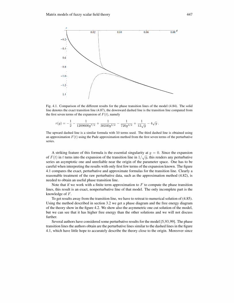
Matrix models of fuzzy scalar field theory 447
Fig. 4.1. Comparison of the different results for the phase transition lines of the model (4.84). The solidline denotes the exact transition line (4.87), the downward dashed line is the transition line computed fromthe first seven terms of the expansion of F (t), namely
r(g) = −1
2− 1
1209600g7/2+
1
30240g5/2− 1
720g3/2+
1
12√
g− 4√
g .
The upward dashed line is a similar formula with 50 terms used. The third dashed line is obtained usingan approximation F (t) using the Pade approximation method from the first seven terms of the perturbativeseries.
A striking feature of this formula is the essential singularity at g = 0. Since the expansionof F (t) in t turns into the expansion of the transition line in 1/
√g, this renders any perturbative
series an asymptotic one and unreliable near the origin of the parameter space. One has to becareful when interpreting the results with only first few terms of the expansion known. The figure4.1 compares the exact, perturbative and approximate formulas for the transition line. Clearly areasonable treatment of the raw perturbative data, such as the approximation method (4.82), isneeded to obtain an useful phase transition line.
Note that if we work with a finite term approximation to F to compute the phase transitionlines, this result is an exact, nonperturbative line of that model. The only incomplete part is theknowledge of F .
To get results away from the transition line, we have to retreat to numerical solution of (4.85).Using the method described in section 3.2 we get a phase diagram and the free energy diagramof the theory show in the figure 4.2. We show also the asymmetric one cut solution of the model,but we can see that it has higher free energy than the other solutions and we will not discussfurther.
Several authors have considered some perturbative results for the model [5,93,99]. The phasetransition lines the authors obtain are the perturbative lines similar to the dashed lines in the figure4.1, which have little hope to accurately describe the theory close to the origin. Moreover since

448 Phase structure of fuzzy field theories and matrix models
Fig. 4.2. (Color online) The phase diagram and the free energy diagram of the model (4.84) obtainednumerically. The green region denotes the one cut solution, the blue region the two cut solution and the redregion denotes the asymmetric one cut solution, which is easily seen to have higher free energy than thetwo cut solution. The green lines represent the symmetric one cut/asymmetric one cut phase transition, thered lines the symmetric one cut/two cut phase transition and the blue lines the two cut/asymmetric one cutphase transition. The blue line is the analytic transition line (4.87), the dashed line denotes the transitionline of the original model.
no odd terms have been considered in the action, the asymmetric solutions should have a higherfree energy. A region of parameters space where this is not true has been found in [93], but thisis only a relict of the perturbative treatment.
Most recently, perturbative phase structure of the model corresponding to the fuzzy discscalar field theory has been considered [100], including the odd terms. Due to the perturbativetreatment only, we expect the results to be changed in nonperturbative considerations.
4.3.2 Perturbative asymmetric regime
The first attempts to include the asymmetric solution of the matrix model corresponding to theuniform order phase of the field theory was presented in [93]. However the authors consideredonly the symmetric terms in the action, which is not satisfactory for the asymmetric regime.
In [96] a model which included asymmetric terms was analyzed perturbatively. A simple

Matrix models of fuzzy scalar field theory 449
model was considered, with asymmetry introduced by considering the complete asymmetric ver-sion of t2 = c2 − c2
1 in the perturbative expression for F (t). This yields a model
Seff =12F (c2 − c2
1) +12rTr(M2)
+ gTr(M4)
≈12A1(c2 − c2
1) +12A2(c2 − c2
1)2 +
12rTr(M2)
+ gTr(M4)
. (4.89)
The equations determining the asymmetric one cut solution (3.85) are (3.97,3.99)
0 =− 12c1
(A1 + 2A2(c2 − c2
1))
+ 2D3g + 3Dδg
+12D(r + A1 + 2A2(c2 − c2
1))
, (4.90a)
1 =3D2δg +34δ2g
14δ(r + A1 + 2A2(c2 − c2
1))
, (4.90b)
c1 =3D3δg +32Dδ2g +
14Dδ(r + A1 + 2A2(c2 − c2
1))
, (4.90c)
c2 =3D4δg + 3D2δ2g +14δ3g +
14D2δ
(r + A1 + 2A2(c2 − c2
1))+
+116
δ2(r + A1 + 2A2(c2 − c2
1))
. (4.90d)
These are supplemented by the phase transition condition (3.101)
4D2g + 2δg + r + 4Dgx + 4gx2 + A1 + 2A2(c2 − c162) = 0 . (4.90e)
As we have seen in the section 3.3, these equations are beyond any hope to solve analytically.The procedure adopted in [96] was thus to solve them perturbatively in the kinetic term contri-bution. Technically, this meant replacing A1 → εA1, A2 → ε2A2 and looking for solution ofthe equations (4.90) as a power series in ε. Obviously, if we include more terms of the expansionof F (t) in (4.89), one can go further also in the expansion of the solution. The following, ratherlengthy formula, for the transition line has been obtained for the seventh order approximation ofF
r(g) = −2√
15g +4A1
5+(
135A21 + 848A2
1500√
15
)1√
g+ (4.91)
+1g
(2025A3
1 + 11236A3 + 10170A1A2
562500
)+
+1
(√
g)3
(5740875A4
1 + 32464800A21A2 + 19805040A2
2
+29707560A1A3 + 19056256A4
)2025000000
√15
+
+1g2
(19683000A5
1 + 108172665A21A3 + 70685676A1A4 + 31561924A5
+126372150A31A2 + 106028514A3A2 + 144230220A1A
22
)113906250000
+

450 Phase structure of fuzzy field theories and matrix models
+1
(√
g)5
237487696875A6
1 + 1709468550000A41A2 + 2801052738000A2
1A22
+609290035200A32 + 1400526369000A3
1A3 + 2741805158400A1A2A3
+423995740920A23 + 913935052800A2
1A4 + 753770206080A2A4
+471106378800A1A5 + 26764511552A6
1366875000000000
√15
+
+1g3
2391484500000A7
1 + 15074840643750A41A3 + 9480160743525A1A
23
+9749822053500A31A4 + 4512250464660A3A4 + 5266755968625A2
1A5
+376020872055A1A6 + 620602111612A7 + 19049945512500A51A2
+43874199240750A21A3A2 + 16853619099600A1A4A2
+3760208720550A5A2 + 40199575050000A31A
22
+12640214324700A3A22 + 19499644107000A1A
32
192216796875000000
+
+1
(√
g)7
51778255111171875A81 + 451444780593000000A16A2
+1156207911142500000A41A
22 + 886545939600000000A2
1A32
+97520988528864000A42 + 346862373342750000A5
1A3
+1329818909400000000A31A2A3 + 877688896759776000A1A
22A3
+329133336284916000A21A
23 + 170459137959667200A2A
23
+221636484900000000A41A4 + 585125931173184000A2
1A2A4
+151519233741926400A22A4 + 227278850612889600A1A3A4
+23876085465308160A24 + 121901235661080000A3
1A5
+189399042177408000A1A2A5 + 44767660247452800A3A5
+9469952108870400A21A6 + 5969021366327040A2A6
+20891574782144640A1A7 + 4811616828772352A8
3690562500000000000000
√15
.
Note that this formula is also general and does not rely on any particular form of F and can beused for any kinetic term.
It is important to stress that this is not truly a phase transition line yet. It is just a boundaryof the region of existence of the asymmetric one cut solution. It is however not guaranteed thatsuch solution will be realized, as it is not clear where, if at all the free energy of such solution islower than of the symmetric solutions.
Moreover, the character of the expansion is not clear at the moment either. Assuming thatthe series in 1√
g is convergent, one can use the formula (4.91) to obtain an approximate locationof the triple point of the theory. The table 4.1 shows the location of the triple point for differentorders of the perturbative approximation for the fuzzy sphere.
The results for the first few CPn’s are given in the table 4.2. If however the expansion isasymptotic, it is not clear how well or if at all these values approximate the location of the triplepoint. Clearly, a non-perturbative tool is needed.

Matrix models of fuzzy scalar field theory 451
order gc rc
2 0.02091 -0.72213 0.02127 -0.72824 0.0215 -0.73265 0.02171 -0.73566 0.02185 -0.73797 0.02195 -0.73978 0.02204 -0.7412
Tab. 4.1. Comparison of the location of the triple point in the case of the fuzzy sphere for different pertur-bative orders.
n gc rc
1 0.02160 -0.73692 0.1714 -2.0483 0.9320 -5.3334 2.890 -9.7845 6.713 -15.20
Tab. 4.2. Numerical values for the CP nF triple points. The value for n = 1, i.e. the fuzzy sphere, was
obtained using the approximate phase boundary and not using the exact expression.
4.3.3 Non-perturbative asymmetric regime
To obtain the free energy diagram as well as a phase transition line reliable for all values of g,we treat the problem numerically. Starting from the action
S =12F (c2 − c2
1) +12rTr(M2)
+ gTr(M4)
(4.92)
we obtain the saddle point equation
−c1F′(c2 − c2
1) +(r + F ′(c2 − c2
1))λi + 4gλ3
i =2N
∑i 6=j
1λi − λj
. (4.93)
This corresponds to an asymmetric effective single trace model
Seff = aeff Tr (M) +12reff Tr
(M2)
+ gTr(M4)
. (4.94)
To connect it with the model (3.95) we have studied in the section 3.3, we rescale the matrix (oreigenvalues) by x0 = −c1F
′(c2 − c21). Now the model is in the desired form
Seff = Tr (M) +12reff Tr
(M2)
+ geff Tr(M4)
(4.95)
with
reff =r + F ′(c2 − c2
1)x2
0
, geff =g
x40
. (4.96)
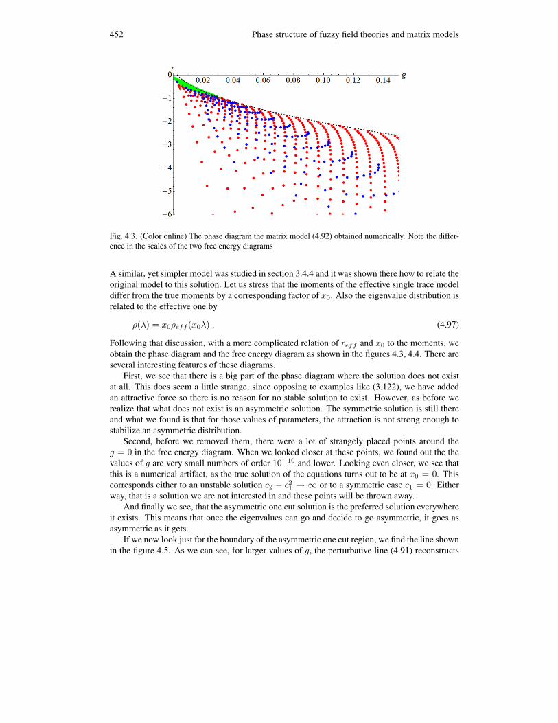
452 Phase structure of fuzzy field theories and matrix models
Fig. 4.3. (Color online) The phase diagram the matrix model (4.92) obtained numerically. Note the differ-ence in the scales of the two free energy diagrams
A similar, yet simpler model was studied in section 3.4.4 and it was shown there how to relate theoriginal model to this solution. Let us stress that the moments of the effective single trace modeldiffer from the true moments by a corresponding factor of x0. Also the eigenvalue distribution isrelated to the effective one by
ρ(λ) = x0ρeff (x0λ) . (4.97)
Following that discussion, with a more complicated relation of reff and x0 to the moments, weobtain the phase diagram and the free energy diagram as shown in the figures 4.3, 4.4. There areseveral interesting features of these diagrams.
First, we see that there is a big part of the phase diagram where the solution does not existat all. This does seem a little strange, since opposing to examples like (3.122), we have addedan attractive force so there is no reason for no stable solution to exist. However, as before werealize that what does not exist is an asymmetric solution. The symmetric solution is still thereand what we found is that for those values of parameters, the attraction is not strong enough tostabilize an asymmetric distribution.
Second, before we removed them, there were a lot of strangely placed points around theg = 0 in the free energy diagram. When we looked closer at these points, we found out the thevalues of g are very small numbers of order 10−10 and lower. Looking even closer, we see thatthis is a numerical artifact, as the true solution of the equations turns out to be at x0 = 0. Thiscorresponds either to an unstable solution c2 − c2
1 → ∞ or to a symmetric case c1 = 0. Eitherway, that is a solution we are not interested in and these points will be thrown away.
And finally we see, that the asymmetric one cut solution is the preferred solution everywhereit exists. This means that once the eigenvalues can go and decide to go asymmetric, it goes asasymmetric as it gets.
If we now look just for the boundary of the asymmetric one cut region, we find the line shownin the figure 4.5. As we can see, for larger values of g, the perturbative line (4.91) reconstructs

Matrix models of fuzzy scalar field theory 453
Fig. 4.4. (Color online) The free energy of the the matrix model (4.92) obtained numerically. Note thedifference in the scales of the two diagrams
Fig. 4.5. The boundary of the asymmetric one cut solution region from the figure 4.4, shown in solid,compared with the perturbative line (4.91), shown in dashed.

454 Phase structure of fuzzy field theories and matrix models
Fig. 4.6. (Color online) Comparison of the symmetric and the asymmetric free energies of the model (4.92).
the solution nicely. But for small values the difference is significant. And gets more significant aswe include more terms in the perturbative expansion (4.91). We thus conclude that the expansionis asymptotic in for small values of g.
We now have all the ingredients needed to obtain the full phase diagram of the theory.
4.3.4 Interplay of the symmetric and the asymmetric regime
To study the interplay of the symmetric and asymmetric regimes, we need to put the free energydiagrams 4.2 and 4.4 on top of each other, which is done in the figure 4.6. And quite to oursurprise, we see that the asymmetric regime is the preferred wherever it is possible. It is asurprise, as the perturbative treatment in [93] suggested otherwise. We thus conclude, that thiswas has probably been a relict of the perturbative approach not present in the full nonperturbativeresults. And we obtain the phase diagram of the theory as in the figure 4.7.
The intersection of the two lines occurs at a critical coupling equal to approximately
gc ≈ 0.02 . (4.98)
We see that this is a little lower than the value in the table 4.1. This is clearly the result of theasymptotic character of the perturbative expansion (4.91).
And the value is smaller roughly by a factor of 7 from the numerical values (2.41) of thenumerical works [81, 82]. To compare better, we draw our phase diagram and the numericalphase diagram in the same picture in the figure 4.8.
We see that the diagrams, together with the location of the triple point are in in a qualitativeagreement, but to claim they agree quantitatively would be a rather bold statement.
One possible source of the discrepancy is clearly the remainder term R in (4.63) which willdeform the transition lines. However there is a possible problem also on the part of the numerics.The lines in the phase diagrams are linear extrapolation of data. And looking at the originalfigure 2.1, we see that the data points are at values in the range r ∈ (0.4, 0.6). This is a littletoo far away from the triple point and the linear extrapolation does not take into account the turn

Matrix models of fuzzy scalar field theory 455
Fig. 4.7. (Color online) The complete phase diagram of the model (4.92). The black line is the numericallyobtained boundary of existence of the asymmetric one cut solution from the figure 4.5. The red line is theanalytic boundary of existence of the symmetric one cut solution (4.87).)
Fig. 4.8. (Color online) The phase transition lines, shown in dashed, which are linear fits to the data points,from the numerical work [81] compared with the phase transition lines presented here. The small rectanglein the top left corner denotes the area covered by the figure 4.7.
the transition lines make for small values of g. As long as this turn is not drastically changedby the higher terms deformation, numerical data do overestimate the triple point. After somepreliminary numerical analysis closer to the origin of the phase diagram, this seems to be thecase, however it is not clear to what extent [101].
456 Phase structure of fuzzy field theories and matrix models
4.4 Phase structure of the fourth moment multitrace model
In this last section, we will study the phase structure of a model with the perturbative effectiveaction (4.60). Moreover, as very little changes if we consider the first part nonperturbatively, wewill use the expression for F (t) rather than the perturbative part. The action includes quarticmultitrace terms, but as we will shortly see, does not explain the phase structure of the fieldtheory.
Again, we will first study the symmetric case and the asymmetric case afterward.
4.4.1 The symmetric regime
The full action for the symmetric regime is
S =12F (c2)−
13456
(c4 − 2c2
2
)2+
12rTr(M2)
+ gTr(M4)
, (4.99)
which is a combination of the nonperturbative part (4.69) obtained in [95] and the perturbativeterm obtained in [94]. The effective parameters are given by
reff = r + F ′(c2) +1
216c2(c4 − 2c2
2) , geff = g − 11728
(c4 − 2c22) . (4.100)
Approaching the problem numerically, we can find the phase diagram and the free energy dia-gram of this model by now familiar method and obtain diagrams show in the figure 4.9.
The free energy diagram has clearly features which we do not expect from the diagram ofthe fuzzy field theory. It allows for a solution for negative g, for some values of g > 0 it has nosolution and it has more than one solution elsewhere. This is the first clue that there is somethingwrong with the interpretation of the perturbative effective action (4.60) as the action of the scalarfield on the fuzzy sphere. But at the moment, let us follow the discussion.
If we are interested only in the phase transition line, the expressions simplify again and weare able to find the line analytically. Plugging (4.100) in (3.83) gives
c2 =−r + F ′(c2) + 1
216c2(c4 − 2c22)
4(g − 1
1728 (c4 − 2c22)) , (4.101a)
c4 =c2 +1
4(g − 1
1728 (c4 − 2c22)) . (4.101b)
which together with reff = −4√geff yields after some algebra
r(g) = − 1
1− e
4√
3√24g+
√1+576g2
+2
√3(24g +
√1 + 576g2
)3/2−
5√
24g +√
1 + 576g2
4√
3,
(4.102)
the line shown in the figure 4.9 together with the transition line (4.87) for the model without thequartic multitrace term. It is important to point out, that this phase transition is exact. Starting

Matrix models of fuzzy scalar field theory 457
Fig. 4.9. (Color online) The phase diagram and the free energy of the the matrix models (4.99). The greenregion denotes the one cut solution, the blue region denotes the two cut solution. The blue line is the exacttransition line (4.102).
from the action (4.99), no perturbative considerations have been made. So as long as this modelsis viewed this formula is complete.
But if the model is viewed as a representation of the fuzzy field theory, the action is a pertur-bative expansion and the given formula is just a perturbative approximation of the true transitionline. And we see again that it is not a good approximation to the true transition line, which isexpected to go through the origin. This is another clue, that the perturbative effective action(4.99), even if the part F (t) is taken nonperturbatively, is not a good starting point to the analysisof phase structure of the fuzzy field theory.
For completeness though, let us continue with the discussion of the consequences of theperturbative effective action to its bitter end with the asymmetric regime.

458 Phase structure of fuzzy field theories and matrix models
To compare with the asymmetric results we will obtain shortly, we shall compute the tran-sition line also perturbatively. We will take the expansion of F up to the fourth order (to beconsistent with the fourth order of the other term) and obtain the transition line
r = −4√
g − 12
+1
12√
g+
75760g3/2
+29
1935360g5/2. (4.103)
Note, that this formula agrees with the first terms in the 1/√
g expansion of (4.102).
4.4.2 The asymmetric regime
The full action for the asymmetric regime is again the combination of the perturbative part (4.60)and the non-perturbative part (4.69), but now with all the odd terms included
S =12F (c2 − c2
1)−1
3456
[(c4 − 4c3c1 + 6c2c
21 − 3c4
1)− 2(c2 − c21)
2]2−
− 1432
(c3 − 3c1c2 + 2c3
1
)2+
12r Tr
(M2)
+ g Tr(M4)
. (4.104)
This action leads to the following saddle point equation[1
432
(− 25c7
1 + 3c51(25c2 − 8)− 25c4
1c3 + 6c21(5c2 − 2)c3 + c3(6c2 − 2c2
2 + c4)
+c31(48c2 − 60c2
2 + 5c4) + c1(10c32 − 18c2
2 − 4c23 − 5c2c4)
)− c1F
′(c2 − c21)]+
+[
1432
(25c6
1 + c41(24− 60c2)− 4c3
2 + 20c31c3 + 4c1(3− 2c2)c3+
+c21(30c2
2 − 36c2 − 5c4) + 2c2c4
)+ F ′(c2 − c2
1) + r
]λi+
+[
1144
(− 5c5
1 + 2c31(5c2 − 2)− 2c3 − 4c2
1c3 + c1(6c2 − 2c22 + c4)
)]λ2
i +
+[
1432
(5c4
1 − 10c21c2 + 2c2
2 + 4c1c3 − c4
)+ 4g
]λ3
i =2N
∑i 6=j
1λi − λj
,
(4.105)
which we will, for the brevity of the equations, write as
X0 + (r + X1)λi + X2λ2i + (4g + X3)λ3
i =2N
∑i 6=j
1λi − λj
. (4.106)
This equation leads to an effective single trace matrix model which is not of the form (3.95),since the λ2 term leads to a Tr
(M3)
term in the action of the effective model. We can howeverget rid of such term by shifting the matrix M . By changing M → (M − a id)/x0, where
x0 =X0 +2X3
2
27(4g + X3)2− (r + X1)X2
3(4g + X3), (4.107a)

Matrix models of fuzzy scalar field theory 459
a =X2
3(4g + X3), (4.107b)
and after dropping the constant term, we obtain the effective single trace matrix model in thedesired form (3.95)
S = Tr (M) +12reff Tr
(M2)
+ geff Tr(M4)
, (4.108)
with
reff =12g(r + X1)−X2
2 + 3(r + X1)X3
3(4g + X3)x20
, (4.109a)
geff =4g + X3
4x40
. (4.109b)
Moreover, the moments of the distribution cn, which are to be used when evaluating X’s arerelated to the moments of the effective single trace matrix model distribution (3.99) by
c1 =c1,eff
x0− a
x0, (4.110a)
c2 =c2,eff
x20
− 2c1,effa
x20
+a2
x20
, (4.110b)
c3 =c3,eff
x30
− 3c2,effa
x30
+3c1,effa2
x30
− a3
x30
, (4.110c)
c4 =c4,eff
x40
− 4c3,effa
x40
+6c2,effa2
x40
− 4c1,effa3
x40
+a4
x40
. (4.110d)
Unfortunately there is little we can do with our approach in this case. If we choose particularvalues of reff and geff , the moments of the effective single trace model are known and theequations to be solved numerically are (4.107) plugged into (4.110) together with (4.109). Thissystem is way too complicated to be handled. So to include the effect of the new terms, we retreatto the perturbative calculation and repeat the procedure of [96].
This means we reintroduce the parameter ε and solve the equations determining the solutionas a series in powers of ε, later setting ε = 1. The final result we obtain is
r(g) = −2√
15√
g25− 19
18000√
15√
g+
291125000g
− 78861834374000000000
√15g3/2
. (4.111)
We stress that this formula is a perturbative one even if the model (4.104) is viewed as a completeaction. We cannot do much more here, so we continue to the comparison of the two regimes.
4.4.3 The interplay of the perturbative symmetric and asymmetric regimes
The figure 4.4.3 shows a little sad plot of the symmetric transition lines (4.103) and (4.102) withthe asymmetric transition line (4.111). These transition lines do not intersect and the perturbativemodel as it stands does not have a triple point. Also, recalling the free energy diagram of the

460 Phase structure of fuzzy field theories and matrix models
Fig. 4.10. (Color online) The phase transition lines (4.102) - the red solid line,(4.103) - the red dashed lineand (4.111) - the black line in one figure, showing the incompleteness of the perturbative description.
symmetric regime in the figure 4.9, the phase structure of such model is not clear at all and surelydoes not represent the phase structure discussed in the section 2.3.
We thus conclude, that the phase structure of the fuzzy field theory is very sensitive to theterms of the perturbative expansion. To be able to make any reasonable statements about theproperties of the phase diagram of the field theory, once we include some multitrace term, weneed to include terms of all orders in that moment. A similar result has been obtained recentlyin a Monte-Carlo study of the perturbative multitrace model (4.104) in [102], where it is shownthat the perturbative version of the model (4.99) does not reconstruct the phase structure of thefuzzy field theory. It would be interesting to see, how our results connect to this work.

Conclusions and outlook 461
5 Conclusions and outlook
We have presented an application of the matrix model techniques to the study of the phase struc-ture of the scalar field theory on the fuzzy sphere. Our goal was to reproduce the available resultsof various numerical simulations. We have analyzed two different models, which approximatethe field theory in two different ways.
One of the models did a decent job, reproducing the expected qualitative features of thediagram and giving a reasonable quantitative values of the parameters of the diagram. The secondmodel did much worse and have been neither in qualitative nor quantitative agreement with theexpectations. As we have seen, the key property distinguishing these two models and leadingto the success or the failure was the fact that the approximation used in the first model was anonperturbative. And the fact, that the second approximation was in some sense more precise, asit included several extra terms, played little role.
So the main lesson we have learned is that if one uses a matrix model to approximate thefuzzy field theory, it is very important that the terms are arranged in a nonperturbative packing.Perturbative approximations are of little use if we aim to explain the phase structure of the theory.
We will now conclude our journey with several open questions or interesting related prob-lems. We start with a short remainder, that we have left two loose ends on the numerical sideof our work. One should try to improve the algorithm for the treatment of the two cut solutionof the asymmetric quartic model and come up with a better numerical treatment of the second,perturbative approximation matrix model, capable of handling the t3 term.
The kinetic term effective actionWe do not have to go too far for the further problems. Some better, perhaps a complete
treatment of the angular integral (4.3) is desirable. Unfortunately, there are very few hints on howto approach this problem further, as the perturbative treatment seems to be way too complicated[94] and there is no hint how to generalize the nonperturbative treatment of [95] beyond thesecond moment. The reason might be that we are on a wrong track. The moments, in whichwe try to express the kinetic term effective action, might not be the most useful variable. Theeffective action is a function of the eigenvalues and the moments are perhaps a bad way how toexpress this dependence. For example if we tried to express the repulsive Vandermonde termin terms of the moments, we would very soon run into difficulties. So stopping for a while andrethinking the whole problem over might bring some new insight.
Nonperturbative approximation of perturbative approximationWe have presented a possible method how to pack a perturbative expansion into a nonper-
turbative form, yielding a nonperturbative approximation of perturbative approximation. Eventhough still an approximation, it might be useful for computations. We have very little informa-tion of about the remainder termR (4.63) so the method based on Pade approximants is not veryuseful, but we still can cook up an approximation by
R =− 1432
t23 −1
3456(t4 − 2t22
)2 ≈ log[h
(1
432, t3
)h
(1
3456, t4 − 2t22
)], (5.1)
where

462 Phase structure of fuzzy field theories and matrix models
h(α, x) ∼ −αx2 x→ 0log x x→∞ (5.2)
for example
h(α, x) =1
1 + (1 + α) x2+
x2
1 + x, (5.3)
h(α, x) =e−(1+α)x2+ x
(1− e−x
). (5.4)
It would definitely be interesting to study a matrix model with such multitrace term.
Other noncommutative spacesAs mentioned in the text, there are numerical results available for several other spaces, the
fuzzy disc [77], three dimensional case of R× S2F [75], noncommutative plane [76] to name
some. Moreover, for the first there is a perturbative analysis available also [103] and for thesecond an perturbative approximation similar to the one studied here [100]. The fuzzy disceffective action includes the linear c4 term and also does not vanish for the semicircle. It wouldbe very interesting to generalize the nonperturbative treatment of the section 4.2.3 to these spacesand see how these results compare.
Also, we could clearly do computations for different spaces, where no previous results areavailable, such as CP 2, CP 3, a general CPn or the fuzzy foursphere S4 [50]. Moreover, if oneconsiders a general φ2k theory and repeat the procedure of the section, one could look for theaspects of non-renormalizability of certain theories, like φ6 on R4 or φ4 on R6, that are reflectedin the regularized matrix versions. This was suggested in [5] and [93], but was not elaborated onneither there, nor here. Some very interesting structure of M6 matrix model is revealed in [104]and the straightforward connection of this model to the φ6 theory conjectured here makes thoseresults relevant.
Phase structure of the UV/IR free theoriesAnd finally, the most interesting problem. As mentioned in the text, there are several mod-
ifications of the naive versions of the scalar field theory which remove the UV/IR mixing phe-nomenon. Both for the fuzzy sphere and for Euclidean spaces [66, 67, 105]. The phase structureof such spaces is of prime interest, as the non-uniform order phase should be removed togetherwith the UV/IR mixing. This remains to be shown and perhaps one could learn something newfrom the way the extra phase is removed.
Beyond noncommutative field theoryUndoubtedly, there is a lot of possibility to apply the results for the asymmetric quartic model
and the multitrace models beyond the phase structure of the noncommutative field theories, asthe idea has been successfully used before [106, 107, 108]. Interestingly, a similar matrix modelappears also in the study of the random geometry on the fuzzy sphere [109].
Acknowledgement: I would like to thank Denjoe O’Connor for useful discussions. This workwas supported by the Alumni FMFI foundation as a part of the Navrat teoretikov project.
Description of the numerical algorithm 463
A Description of the numerical algorithm
In this section, we will present the algorithm used to numerically solve the equations (3.107,3.110e) for the asymmetric two cut solution of the model (3.95). Trying to use numerical methodsof the computer algebra program directly on the equation (3.110e) yields little success, so wewere forced to come up with something else.
The algorithm starts with choosing some particular values of r and g as before. Then we takethe value of D2 to be −D1(1 + x), where x is our new parameter. We chose a particular valueof x and solve the equations (3.107) numerically using standard features of the computer algebraprogram. Again, navigating our way through handful of irrelevant solutionsA.1, we check for thevalue of (3.110e) for the relevant solution (if it exists).
Doing this, we scan through a reasonable interval of x observing when does the value changesign. When we find an interval of x with different sign of (3.110e) at the endpoint, we zoomto this area and look further. We again split the interval into parts and look for the change ofsign. When we find such interval, we take a linear approximation to the function given by thevalues at the endpoints and take the root of this linear fit as the solution for x and thus for all theparameters D1,2 and δ1,2.
We have used the following values for our search. Interval of x has been (0, 0.3), whichwas first split into 500, 300, 100 or 50 parts, depending on the values of r and g. Generally, forsmall g larger number was needed to find the solution. If the solution has not been found forsmaller value of the number, the algorithm ran again with the value of 500 to make sure thereis no solution. This way we achieved a balance between precision and speed. The part wherethe value of (3.110e) has changed sign was divided further into 50 parts. We then chose for ourvalue of x the midpoint of the small interval where (3.110e) changes sign. The program hadtrouble when the edge of the first interval was too close to the zero, so if the value of (3.110e)was too close to zero (absolute value smaller than 0.5) in our program, we have narrowed downthe second interval.
The biggest problem of the algorithm was the exact location of the transition line betweenthe asymmetric one cut and the two cut solution. We did our best to tune the parameters ofthe algorithm to achieve good precision while having a reasonable speed, but there still mightbe points around the boundary which we have missed. Clearly, there is also a lot of room forimprovement of the speed of this algorithm. However for the current purposes this version didserve quite well.
A.1These are imaginary solutions, solutions with negative δ’s and solutions where the two intervals overlap.

464 Phase structure of fuzzy field theories and matrix models
References
[1] H. Steinacker, “A Non-perturbative approach to non-commutative scalar field theory,” JHEP 0503,075 (2005) [hep-th/0501174].
[2] H. Steinacker, “Quantization and eigenvalue distribution of noncommutative scalar field theory,”[hep-th/0511076].
[3] H. Steinacker, “Quantized gauge theory on the fuzzy sphere as random matrix model,” Nucl. Phys.B 679, 66 (2004).
[4] V.P. Nair, A.P. Polychronakos, J. Tekel, “Fuzzy spaces and new random matrix ensembles,” Phys.Rev. D 85, 045021 (2012) [1109.3349 [hep-th]].
[5] D. O’Connor, C. Samann, “Fuzzy Scalar Field Theory as a Multitrace Matrix Model,” JHEP 0708,066 (2007) [0706.2493 [hep-th]].
[6] A. Connes, “Noncommutative Geometry,” (Academic Press, 1994).[7] G. Landi, “An Introduction to Non-commutative Spaces and their Geometry,” (Springer-Verlag,
1997).[8] H.S. Snyder, “Quantized Spacetime,” Phys. Rev. 71 (1947) 38.[9] S. Doplicher, K. Fredenhagen, J.E. Roberts, “The quantum structure of spacetime at the Planck scale
and quantum fields,” Comm. Math. Phys. 172 (1995), no. 1, 187-220.[10] A. Connes, J. Lott, “Particle models and non-commutative geometry,” Nucl. Phys. (Proc. Suppl.)
18B (1991) 29.[11] D. Kastler, T. Schucker, “A detailed account of Alain Connes’ version of the standard model,” Rev.
Math. Phys. 8 (1996) 205.[12] A. Connes, M. Marcolli “Noncommutative Geometry, Quantum Fields and Motives,” Preliminary
version under revision.[13] W. van Suijlekom, “Noncommutative Geometry and Particle Physics,” Springer Netherlands, 2015.[14] A. Chamseddine, G. Felder and J. Frohlich, “Gravity in non-commutative geometry,” Commun.
Math. Phys. 155 (1993) 205.[15] G. Landi and C. Rovelli, “Gravity from Dirac eigenvalues,” Phys. Rev. Lett. 78 (1997) 3051.[16] D. Karabali and V. P. Nair, “Quantum Hall effect in higher dimensions,” Nucl. Phys. B 641 (2002)
533 .[17] D. Karabali and V.P. Nair, “Quantum Hall Effect in Higher Dimensions, Matrix Models and Fuzzy
Geometry,” J. Phys. A: Math. Gen. 39 (2006) 12735.[18] B. Morariu, A.P. Polychronakos, “Quantum mechanics on non-commutative Riemann surfaces,”
Nucl. Phys. B 634 (2002) 326.[19] D. Karabali, V.P. Nair, A.P. Polychronakos, “Spectrum of Schrodinger field in a non-commutative
magnetic monopole,” Nucl.Phys. B627 (2002) 565.[20] V. Schomerus, “String Theory and Noncommutative Geometry,” JHEP 09 (1999) 032, [hep-
th/9903205].[21] N. Seiberg, E. Witten, “D-branes and Deformation Quantization,” JHEP 06 (1999) 030 [hep-
th/9908142].[22] M.R. Douglas and N.A. Nekrasov, “Non-commutative field theory,” Rev. Mod. Phys. 73 (2001) 977;[23] R.J. Szabo “Quantum Field Theory on Noncommutative Spaces,” Phys. Rept. 378 (2003) 207 [hep-
th/0109162].[24] D. Kabat, W. Taylor, “Linearized supergravity from Matrix theory,” Phys.Lett.B 426 (1998) 297.

References 465
[25] V.P. Nair and S. Randjbar-Daemi, “On Brane Solutions in M(atrix) Theory,” Nucl. Phys. B 533(1998) 333.
[26] W. Taylor, “M(atrix) Theory: Matrix Quantum Mechanics as a Fundamental Theory,” Rev. Mod.Phys. 73 (2001) 419.
[27] Y. Abe, “Construction of Fuzzy Spaces and Their Applications to Matrix Models,” Ph. D. thesis,Physics Department, City College of New York (2001).
[28] M. Panero, “Quantum Field Theory in a Non-Commutative Space: Theoretical Predictions and Nu-merical Results on the Fuzzy Sphere,” SIGMA 2, (2006), 08 [hep-th/0609205].
[29] W. Bietenholz, F. Hofheinz, H. Mejıa-Dıaz, M. Panero, “Scalar fields on a non-commutative space,”[hep-th/1402.4420].
[30] “Applications of random matrix theory to condensed matter and optical physics,” The Oxford Hand-book of Random Matrix Theory, edited by G. Akemann,J. Baik, P. Di Francesco (Oxford UniversityPress, 2011).
[31] E. Wigner, “Characteristic Vectors of Bordered Matrices with Infinite Dimensions,” Ann. Math. 62(1955) 548.
[32] E. Wigner, “On the Distribution of the Roots of Certain Symmetric Matrices,” Ann. Math. 67(1958)325.
[33] M.L. Mehta “Random Matrices,” 3d edition (Elsevier 2004).[34] G. ’t Hooft, “A planar diagram theory for strong interactions,” Nucl. Phys. B 72 (1974) 461.[35] L. Alvarez-Gaume, “Random surfaces, statistical mechanics and string theory,” Lausane lectures
(1990).[36] M. Marino, “Les Houches lectures on matrix models and topological strings,” hep-th/0410165.[37] P. Di Francesco, “2D Quantum Gravity, Matrix Models and Graph Combinatorics,” math-
ph/0406013.[38] P. Ginsparg and G. Moore, ”Lectures on 2D gravity and 2D string theory”, TASI lectures (1992).[39] C.W.J. Beenakker, “Applications of random matrix theory to condensed matter and optical physics,”
The Oxford Handbook of Random Matrix Theory, edited by G. Akemann,J. Baik, P. Di Francesco(Oxford University Press, 20011).
[40] T. Guhr, A. Muller-Groeling and H.A. Weidenmuller, “Random Matrix Theories in QuantumPhysics: Common Concepts,” Phys. Rep. 299, 189 (1998).
[41] Les Houches, “Chaos and quantum systems,” (Elsevier 1991).[42] P. Bourgade and J.P. Keating, “Quantum chaos, random matrix theory, and the Riemann ζ-function,”
Seminaire Poincare XIV, 115 (2010).[43] A.M Odlyzko “The distribution of spacings between zeros of the zeta function,” Math. Comput. 48
(1987) 273.[44] J. Keating, N.C. Snaith, “Random matrix theory and ζ(1/2 + it),” Comm. Math. Phys. 214 (2000)
57.[45] J. Madore, “An Introduction to Non-commutative Differential Geometry and its Physical Applica-
tions,” (Cambridge University Press, Cambridge - 1995).[46] J. Madore, “The Fuzzy sphere,” Class.Quant.Grav. 9 (1992) 69.[47] H. Grosse, C. Klimcık, P. Presnajder, “Towards Finite Quantum Field Theory in Non-Commutative
Geometry,” Int.J.Theor.Phys. 35 (1996) 231.[48] H. Grosse, C. Klimcık, P. Presnajder, “Topologically nontrivial field configurations in noncommuta-
tive geometry,” Commun.Math.Phys. 178 (1996) 507.[49] Y. Abe, “Construction of fuzzy S4,” Phys. Rev. D 70 (2004) 126004.

466 Phase structure of fuzzy field theories and matrix models
[50] J. Medina, D. O’Connor, “Scalar Field Theory on Fuzzy S4,” JHEP 11 (2003) 051 [hep-th/0212170].[51] D. Karabali, V.P. Nair and R. Randjbar-Daemi, “Fuzzy spaces, the M(atrix) model and the quantum
Hall effect,” in From Fields to Strings: Circumnavigating Theoretical Physics, Ian Kogan Memo-rial Collection, M. Shifman, A. Vainshtein and J. Wheater (eds.) (World Scientific, 2004) [hep-th/0407007].
[52] V.P. Nair, “Noncommutative mechanics, Landau levels, twistors and Yang-Mills amplitudes,” Lec-ture Notes in Physics 698 (Springer-Verlag, Berlin, Heidelberg, 2006).
[53] H. Grosse, H. Steinacker, “Finite Gauge Theory on Fuzzy CP 2,” Nucl. Phys B 707 (2005) 145-198.[54] G. Alexanian, A.P. Balachandran, G. Immirzi, B. Ydri, “Fuzzy CP**2,” J. Geom, Phys, 42 (2002)
28[55] A.M. Perelomov “Generalized Coherent States and Their Applications,” (Springer-Verlag, 1996).[56] A.P. Balachandran, B.P. Dolan, J. Lee, X. Martin, D. O’Connor, “Fuzzy complex projective spaces
and their star products,” J. Geom, Phys, 43 (2002) 184.[57] V.P. Nair, “Gravitational fields on a non-commutative space,” Nucl. Phys B, 651 (2003) 313.[58] D. Karabali, V.P. Nair “The effective action for edge states in higher dimensional quantum Hall
systems,” Nucl.Phys. B 679 (2004) 427.[59] H. Steinacker, “Non-commutative geometry and matrix models,” Proceedings of Science (QGQGS
2011) 004.[60] M. Bordemann, E. Meinrenken and M. Schlichenmaier, “Toeplitz quantization of Kahler manifolds
and gl(N), N →∞ limits,” Commun. Math. Phys. 165 (1994) 281.[61] M. Kontsevich, “Deformation quantization of Poisson manifolds, I,” Lett. Math. Phys. 66 (2003)
157.[62] A.P. Balachandran, S. Kurkcuoglu and S. Vaidya, “Lectures on Fuzzy and Fuzzy SUSY Physics,”
[hep-th/0511114].[63] S. Minwalla, M. Van Rammsdonk, N. Seinberg, “Non-commutative perturbative dynamics,” JHEP 2
(2000) 020 [hep-th/9912072].[64] C.S. Chu, J. Madore, H. Steinacker, “Scaling limits of the fuzzy sphere at one loop,” JHEP 3 (2005)
075.[65] S. Vaidya and B. Ydri, “On the Origin of the UV-IR Mixing in Noncommutative Matrix Geometry,”
Nucl. Phys. B 671 (2003) 4.[66] B.P. Dolan, D. O’Connor, and P. Presnajder, “Matrix φ4 Models of the Fuzzy Sphere and their
Continuum Limits,” JHEP 03 (2002) 013 [hep-th/0109084].[67] H. Grosse, R. Wulkenhaar, “Renormalization of φ4-theory on noncommutative R4 in the matrix
base,” Commun.Math.Phys. 256 (2005) 305 [hep-th/0401128].[68] T.R. Govindarajan, S. Digal, K.S. Gupta, X. Martin, “Phase strucutres in fuzzy geometries,” Pro-
ceedings of Science (CORFU 2011) 058.[69] G.S. Gubser, S.L. Sondhi, “Phase structure of non-commutative scalar field theories,” Nucl. Phys. B
605 (2001) 395.[70] J. Medina, “Fuzzy Scalar Field Theories: Numerical and Analytical Investigations,” Ph. D. thesis,
Physics Department, Instituto Politecnico Nacional, Mexico City (2006)[71] J. Glimm, A.M. Jaffe, “Phase transition for φ4
2 quantum fields,” Comm. Math. Phys. 45 (1975),203-216.
[72] W. Loinaz, R.S. Willey, “Monte Carlo Simulation Calculation of Critical Coupling Constant forContinuum φ4
2,” Phys. Rev. D 58 (1998) 076003 [hep-lat/9712008].

References 467
[73] A.P. Balachandran, T.R. Govindarajan, B. Ydri, “The Fermion Doubling Problem and Non-commutative Geometry,” Mod. Phys. Lett. A15 (2000) 1279.
[74] G.H Chen, Y.S. Wu, “Renormalization group equations and the Lifshitz point in non-commutativeLandau-Ginsburg theory,” Nucl. Phys. B 6022 (2002) 189.
[75] J. Medina, W. Bietenholz, D. O’Connor, “Probing the fuzzy sphere regularization in simulations ofthe 3d λφ4 model,” JHEP 04 (2008) 041 [0712.3366 [hep-th]].
[76] H. Mejıa-Dıaz, W. Bietenholz, M. Panero, “The Continuum Phase Diagram of the 2d Non-Commutative λφ4 Model,” JHEP 1410 (2014) 56. [1403.3318 [hep-lat]].
[77] F. Lizzi, B. Spisso, “Noncommutative Field Theory: Numerical Analysis with the Fuzzy Disc,”Int.J.Mod.Phys. A27 (2012) 1250137, [1207.4998 [hep-th]].
[78] X. Martin, “A matrix phase for the φ4 scalar eld on the fuzzy sphere,” JHEP 04 (2004) 77.[79] M. Panero, “Numerical simulations of a non-commutative theory: the scalar model on the fuzzy
sphere,” JHEP 05, 082 (2007) [hep-th/0608202].[80] F. Garcıa-Flores, X. Martin, D. O’Connor, “Simulation of a scalar field on a fuzzy sphere,” Proceed-
ings of Science LAT 2005 (2006) 262 [hep-lat/0601012].[81] F. Garcıa-Flores, X. Martin, D. O’Connor, “Simulation of a scalar field on a fuzzy sphere,” Internat.
J. Modern Phys. A 24 (2009), 3917−3944 [0903.1986 [hep-lat]].[82] B. Ydri, “New Algorithm and Phase Diagram of Noncommutative Φ4 on the Fuzzy Sphere,” JHEP
03, 065 (2014) [1401.1529 [hep-th]].[83] B. Eynard, “An introduction to Random Matrices,” Saclay Lecture Notes (2001).[84] B. Eynard, T. Kimura, S. Ribault “Random matrices,” [1510.04430 [math-ph]][85] A. Guionnet, “On Random Matrices,” Lecture Notes in Mathematics (Springer, New York 2008).[86] A. Edelman, N. Raj Rao, “Random Matrix Theory,” Acta Numerica (2005), 1.[87] E. Brezin, C. Itzykson, G. Parisi, J.B. Zuber, “Planar diagrams,” Commun.Math.Phys. 59 (1978).[88] Y. Shimamune, “On the Phase Structure of Large N Matrix Models and Gauge Models,” Phys.Lett.
B 108 (1982) 407.[89] S.R. Das, A. Dhar, A.M. Sengupta, S.R. Wadia, “New Critical Behavior in d = 0 Large N Matrix
Models,” Mod.Phys.Lett. A 5 (1990) 1041-1056.[90] C. Itzykson, J.B. Zuber, “The planar approximation. II,” J. Math. Phys. 21 (1980) 411.[91] A.O. Shishanin, “Phases of the Goldstone multitrace matrix model in the large-N limit,”
Theor.Math.Phys. 152 (2007) 1258-1265.[92] J. Tekel, “Random matrix approach to scalar field on fuzzy spaces,” Phys. Rev. D 87, 085015 (2013)
[1301.2154 [hep-th]].[93] C. Samann, “The Multitrace Matrix Model of Scalar Field Theory on Fuzzy CP n,” SIGMA 6 (2010)
[1003.4683 [hep-th]].[94] C. Samann, “Bootstrapping Fuzzy Scalar Field Theory,” JHEP 04 (2015) 044 [1412.6255 [hep-th]].[95] A.P. Polychronakos, “Effective action and phase transitions of scalar field on the fuzzy sphere,” Phys.
Rev. D 88, 065010 (2013) [1306.6645 [hep-th]].[96] J. Tekel, “Uniform order phase and phase diagram of scalar field theory on fuzzy CP n,” JHEP 1410
(2014) 144 [1407.4061 [hep-th]].[97] G.A. Baker, P. Graves-Morris, “Pade Approximants,” Cambridge University Press, 1996.[98] J. Tekel, “Matrix model approximations of fuzzy scalar field theories and their phase diagrams,”
submitted to JHEP, [1510.07496 [hep-th]].[99] B. Ydri, “A Multitrace Approach to Noncommutative Φ4
2,” [1410.4881 [hep-th]].

468 Phase structure of fuzzy field theories and matrix models
[100] S. Rea, Ch. Samann, “The Phase Diagram of Scalar Field Theory on the Fuzzy Disc,” submitted toJHEP, [1507.05978 [hep-th]].
[101] D. O’Connor, private communiation.[102] B. Ydri, K. Ramda, A. Rouag, “Phase diagrams of the multitrae quartic matrix models of noncom-
mutative Φ4,” [1509.03726 [hep-th]].[103] M. Ihl, Ch. Sachse, C. Samann, “Fuzzy Scalar Field Theory as Matrix Quantum Mechanics,” JHEP
03 (2011) 091 [1012.3568 [hep-th]].[104] K. Demeterfi, N. Deo, S. Jain, Ch.I. Tan, “Multiband structure and critical behavior of matrix mod-
els,” Phys. Rev. D 42 (1990) 4105.[105] R. Gurau, J. Magnen, V. Rivasseau, A. Tanasa, “A translation-invariant renormalizable non-
commutative scalar model”, Commun.Math.Phys. 287 (2009) 275 [0802.0791 [math-ph]].[106] I. Andri, L. Jonke, D. Jurman, H.B. Nielsen, “Homolumo Gap from Dynamical Energy Levels”,
Phys. Rev. D 77 (2008) 127701.[107] N. Deo, “Glassy random matrix models,” Phys. Rev. E 65 (2012) 056115.[108] G.S. Krishnaswami, “Phase transition in matrix model with logarithmic action: toy-model for gluons
in baryons,” JHEP 03 (2006) 067.[109] J.W. Barrett, L. Glaser, “Monte Carlo simulations of random non-commutative geometries,”
[1510.01377 [gr-qc]].

Juraj Tekel has earned his master degree in the theoretical and mathematicalphysics at the Faculty of Mathematics, Physics and Informatics of the Come-nius University in Bratislava. After the doctoral studies at the City Universityof New York under the supervision of V.P. Nair he returned to his Alma mater.He works there as a research and teaching assistant and is the Alumni FMFIFoundation fellow in the Navrat teoretikov project. Apart from his main re-search interest, which is the noncommutative field theory and matrix models,
his activities include popularization of physics and science in general and work with talentedyouth.