non-commutative symplectic nq-geometry and courantalgebroids
TRANSCRIPT

UNIVERSIDAD AUTONOMA
Instituto de Ciencias Matemáticas y Departamento de MatemáticasUniversidad Autónoma de Madrid
Non-commutativesymplectic NQ-geometry
andCourant algebroids
Memoria de Tesis Doctoral presentada porDavid Fernández Álvarez
para optar al título de Doctor en Ciencias Matemáticas
Dirigida porDr. Luis Álvarez Cónsul
Noviembre 2015


A mis Padres

That long black cloud is comin’ down,I feel like I’m knockin’ on heaven’s door.
Knock, knock, knockin’ on heaven’s door,Knock, knock, knockin’ on heaven’s door.
Bob Dylan

Agradecimientos
No han sido años fáciles. Supongo que nunca los son. He conocido el sabor deldesánimo, del desaliento, de la incertidumbre, casi de la desesperación. Tambiénhe saboreado la emoción por el descubrimiento, por ir un paso más allá, en defini-tiva, por sacar lo mejor de mí mismo. Quizás haya aprendido a hacerme mayor;lo que seguro que he aprendido es que la vida iba en serio. Creo que en algunosaspectos he ganado como persona; pero me temo haber perdido en otros. Esperoque el balance salga positivo. Pero, sobre todo, estos años se han convertido en uncamino de aprendizaje y éste es el momento de recordar a las personas que me handado tanto y me han permitido completarlo.
Muchas gracias, Luis, por ser mi director, por creer en mí y por confiar en quepodíamos salir vivos de esta aventura. Gracias por tantos momentos en la pizarra,por tu entusiasmo y por tu paciencia. De ti he aprendido que hay que disfrutartrabajando, a hacerse siempre una pregunta más y a que el trabajo está acabadocuando es perfecto. A tu lado he aprendido muchas Matemáticas pero, sobre todo,he aprendido una forma de mirar la Ciencia y la Vida. A partir de ahora, creoque muchas veces me sorprenderé pensando ¿Cómo lo haría Luis? Con esta tesis,pierdo un director pero gano un amigo. Creo que no es mal cambio.
Demasiadas veces, los lugares nos determinan más de lo que nos gustaría re-conocer pues la nostalgia es pegajosa. Yo he tenido la suerte de pertenecer a dosfantásticas instituciones como la Universidad Autónoma de Madrid y el Institutode Ciencias Matemáticas que me han proporcionado el entorno ideal para desar-rollarme como matemático y quizás también como persona. En especial, quieroagradecer a la Universidad Autónoma de Madrid y al Departamento de Matemáti-cas que confiaran en mí y me concedieran una Beca FPI-UAM que me ha permi-tido cumplir mi sueño de convertirme en matemático. Durante este tiempo mehe cruzado con mucha gente y quiero creer que de todos he aprendido algo; desu inteligencia, de su actitud, de sus manías y de sus chistes on the rocks. Enespecial, agradezco a mis compañeros de despacho tantas conversaciones, confiden-cias y risas. Gracias a Juan, Carlos, Diana Carolina, Giuseppe, Marta, Diana,Eugenia, Begoña y Sebastián por haber convertido la rutina en algo placentero.En especial, gracias a Luis Daniel y a Mari Luz por aguantarme y por hacermemejor persona. También agradezco a algunos profesores que se han convertido enun ejemplo para mí: David, Ana, Carlos, Fernando, Orlando, Alberto, José Igna-
v

cio, Tomás, Amparo, Ángel, Enrique, Rafa, Ramón, Manuel, Carmen, Angélica yMario, mi hermano mayor, del que tanto me queda por aprender. En especial, migratitud a mi tutor Jesús Gonzalo quien siempre me ha apoyado durante estos añosy a Juan Luis Vázquez por dejarse embarcar en aventuras casi quijotescas y por en-señarme tanto de la vida, y de las Matemáticas y sus circunstancias. Por supuesto,tampoco me quiero olvidar de Marco Zambon, lector de esta tesis, quien siempreha estado interesado en mi trabajo y ha intentado entenderme. Siguiendo conesta cartografía sentimental, he sido feliz en Príncipe de Vergara 60 y en FrancosRodríguez 60 donde tantas tardes hemos soñado y tantas noches hemos quemado.Gracias Gonza, Javi, Sergio y Curro porque no se me ocurren mejores compañerospara este viaje que nos llevará al fin de la noche, claro.
Gracias Ágata por sacar siempre lo mejor de mí y por enseñarme que lo únicoimportante es luchar por ser feliz. Gracias Henar por ser la persona más inquietaque conozco y por involucrarme siempre en tus planes de ensueño que más prontoque tarde cumpliremos. Gracias Álvaro porque desde que nos pasábamos el balónen el García Quintana, seguimos entendiéndonos tan bien aunque ya no estemosen el recreo y nos haya encontrado el verano. Me siento afortunado por haberencontrado un amigo para toda la vida. Gracias a Miguel por ser tan buenapersona y por enseñarme a seguir adelante, sin mirar demasiado las cartas quea uno le han tocado. Pero no te olvides que la baraja nos debe reyes. GraciasMarina por tantos gin-tonics -y los que nos quedan- y por enseñarme que las ideasson más importantes que las consecuencias. Gracias Giancarlo y Elisa por vuestragenerosidad, por acogerme siempre y hacerme sentir uno más de vuestra familia.Desde luego vosotros ya formáis parte de la mía. También espero que mi ahijadoAdriano alguna vez llegue a leer esto y se sienta orgulloso por haberme ayudado consus sonrisas. Gracias a mi familia por apoyarme siempre, casi irracionalmente, enesta aventura. Gracias a mis abuelas por su infinito amor. En especial, no puedodejar de acordarme de mi abuelo Justo quien no pudo ver terminada esta tesis ya quien tanto quise y a quien todos los días echo tanto de menos. Finalmente,infinitas gracias a mis padres porque sin vosotros nunca lo hubiera conseguido,porque sin vosotros no sería nada. Espero poder devolveros algún día una mínimaparte de todo lo que me habéis dado estos años. Prometo dar lo mejor de mí.

Abstract
We propose a notion of non-commutative Courant algebroid that satisfies theKontsevich–Rosenberg principle, whereby a structure on an associative algebra hasgeometric meaning if it induces standard geometric structures on its representationspaces. Replacing vector fields on varieties by Crawley-Boevey’s double derivationson associative algebras, this principle has been successfully applied by Crawley-Boevey, Etingof and Ginzburg to symplectic structures and by Van den Bergh toPoisson structures.
Courant algebroids, introduced in differential geometry by Liu, Weinsteinand Xu, generalize the notion of the Drinfeld double to Lie bialgebroids. Theyaxiomatize the properties of the Courant bracket, introduced by Courant andWeinstein to provide a geometric setting for Dirac’s theory of constrainedmechanical systems. A direct approach to define non-commutative Courantalgebroids fails, because the Cartan identities are unknown in the calculus of non-commutative differential forms and double derivations, so in this thesis we followan indirect method.
Symplectic NQ-manifolds are non-negatively graded manifolds (the gradingis called weight), endowed with a graded symplectic structure and a symplectichomological vector field Q of weight 1. They encode higher Lie algebroid structuresin the Batalin–Vilkovisky formalism in physics, where the weight keeps track of theghost number. Following ideas of Ševera, Roytenberg proved that symplectic NQ-manifolds of weights 1 and 2 are in 1-1 correspondence with Poisson manifoldsand Courant algebroids, respectively. Our method to construct non-commutativeCourant algebroids is to adapt this result to a graded version of the formalism ofCrawley-Boevey, Etingof and Ginzburg.
We start generalizing to graded associative algebras the theories of bi-symplecticforms and double Poisson brackets of Crawley-Boevey–Etingof–Ginzburg and Vanden Bergh, respectively. In this framework, we prove suitable Darboux theoremsfor graded bi-symplectic forms, define bi-symplectic NQ-algebras, and prove a 1-1correspondence between appropriate bi-symplectic NQ-algebras of weight 1 andVan den Berg’s double Poisson algebras. We then use suitable non-commutativeLie and Atiyah algebroids to describe bi-symplectic N-graded algebras of weight2 whose underlying graded algebras are graded-quiver path algebras, in termsVan den Berg’s pairings on projective bimodules. Using non-commutative derivedbrackets, we calculate the algebraic structure that corresponds to symplectic NQ-algebras of this type. By the analogy with Roytenberg’s correspondence forcommutative algebras, we call this structure a double Courant–Dorfman algebra.
vii


Resumen
En esta tesis proponemos una noción de algebroide de Courant no conmutativoque satisface el principio de Kontsevich–Rosenberg, según el cual una estructurasobre un álgebra asociativa tiene significado geométrico si induce las estructurasgeométricas estándar sobre sus espacios de representaciones. Reemplazando loscampos vectoriales sobre variedades por las derivaciones dobles de Crawley-Boeveysobre álgebras asociativas, este principio ha sido aplicado con éxito por Crawley-Boevey, Etingof y Ginzburg para estructuras simplécticas, y por Van den Berghpara estructuras de Poisson.
Los algebroides de Courant, introducidos por Liu, Weinstein y Xu, generalizanla noción de doble de Drinfeld a bialgebroides de Lie, y axiomatizan las propiedadesdel corchete de Courant definido por Courant yWeinstein para dotar de un contextogeométrico a la teoría de Dirac de sistemas mecánicos con ligaduras. Un enfoquedirecto para definir algebroides de Courant no es posible porque las identidadesde Cartan no se conocen en el cálculo de formas diferenciales no conmutativas yderivaciones dobles, así que en esta tesis seguimos un método indirecto.
Las NQ-variedades simplécticas son variedades graduadas no negativamente (lagraduación se llama peso), dotadas con una estructura simpléctica graduada y uncampo vectorial homológico Q de peso 1. Estas estructuras codifican estructurasde algebroide de Lie de orden superior en el formalismo de Batalin–Vilkoviskyen Física, donde los pesos tienen en cuenta el número fantasma. Siguiendoideas de Ševera, Roytenberg probó que las NQ-variedades simplécticas de pesos1 y 2 están en correspondencia 1-1 con variedades de Poisson y algebroides deCourant, respectivamente. Nuestro método para construir algebroides de Courantno conmutativos consiste en adaptar este resultado a una versión graduada delformalismo de Crawley-Boevey, Etingof, Ginzburg.
Empezamos generalizando a álgebras asociativas graduadas las teorías deformas bi-simplécticas y corchetes dobles de Poisson de Crawley-Boevey–Etingof–Ginzburg y Van den Bergh, respectivamente. En este contexto, probamosteoremas de Darboux adecuados para formas bi-simplécticas, definimos NQ-álgebras bi-simplécticas, y probamos una correspondencia 1-1 entre NQ-álgebrasbi-simplécticas apropiadas de peso 1 y álgebras de Poisson dobles de Van denBergh. Entonces usamos algebroides de Lie y de Atiyah adecuados para describirálgebras N-graduadas de peso 2 cuyas álgebras graduadas subyacentes son álgebrasde caminos de carcajs graduados, en términos de emparejamientos de Van den
ix

Bergh sobre bimódulos proyectivos. Usando corchetes derivados no conmutativos,calculamos la estructura algebraica que corresponde a NQ-álgebras bi-simplécticasde este tipo. Por analogía con la correspondencia de Roytenberg para álgebrasconmutativas, llamaremos a esta estructura un álgebra de Courant–Dorfman doble.

Contents
Agradecimientos v
Abstract vii
Resumen ix
1 Introduction 11.1 Geometric structures on representation spaces . . . . . . . . . 11.2 Courant algebroids . . . . . . . . . . . . . . . . . . . . . . . . 41.3 Symplectic NQ-manifolds . . . . . . . . . . . . . . . . . . . . 61.4 Bi-symplectic NQ-algebras . . . . . . . . . . . . . . . . . . . . 71.5 Bi-symplectic NQ-algebras of weight 1 and double Poisson alge-
bras . . . . . . . . . . . . . . . . . . . . . . . . . . . . . . . . 81.6 Bi-symplectic N-algebras of weight 2 . . . . . . . . . . . . . . 91.7 Bi-symplectic NQ-algebras of weight 2 and double Courant–
Dorfman algebras . . . . . . . . . . . . . . . . . . . . . . . . . 111.8 Contents of the thesis . . . . . . . . . . . . . . . . . . . . . . 12
2 Basics on (graded) non-commutative algebraic geometry 172.1 Background on graded algebras and graded modules . . . . . 18
2.1.1 Outer and inner bimodule structures . . . . . . . . . . 242.1.2 Finitely generated projective modules . . . . . . . . . 28
2.2 Basics on Noncommutative Algebraic Geometry . . . . . . . . 292.2.1 (Graded) Non-commutative differential 1-forms . . . . 292.2.2 Graded Double Derivations and Non-commutative differen-
tial forms . . . . . . . . . . . . . . . . . . . . . . . . . 302.2.3 Smoothness . . . . . . . . . . . . . . . . . . . . . . . . 332.2.4 The (iso)morphism bidualΩ1
RA. . . . . . . . . . . . . 34
2.3 Graded double Poisson structures . . . . . . . . . . . . . . . . 352.3.1 Double Poisson algebras of weight −N . . . . . . . . . 352.3.2 Poly-vector fields and the graded double Schouten–
Nijenhuis bracket . . . . . . . . . . . . . . . . . . . . . 382.3.3 Differential double Poisson algebras . . . . . . . . . . 39
2.4 Bi-symplectic structures . . . . . . . . . . . . . . . . . . . . . 402.5 Definition of bi-symplectic associative N-algebras . . . . . . . 41
xi

Contents
2.6 The Kontsevich–Rosenberg principle for bi-symplectic forms . 43
3 Restriction Theorems of Bi-symplectic forms 473.1 The cotangent exact sequence . . . . . . . . . . . . . . . . . . 483.2 Restriction Theorem in weight 0 . . . . . . . . . . . . . . . . 523.3 Restriction Theorem in weight 1 . . . . . . . . . . . . . . . . 61
3.3.1 Background on graded quivers . . . . . . . . . . . . . 623.3.2 Differential forms and double derivations for quivers . 683.3.3 Casimir elements . . . . . . . . . . . . . . . . . . . . . 683.3.4 The bi-symplectic form for a graded double quiver . . 693.3.5 Restriction Theorem in weight 1 for double graded quivers 72
4 Bi-symplectic NQ-algebras of weight 1 774.1 Symplectic NQ-manifolds of weight 1 . . . . . . . . . . . . . . 77
4.1.1 Basics on symplectic polynomial N-algebras . . . . . . 774.1.2 Classification of symplectic polynomial N-algebras . . 804.1.3 Classification of symplectic polynomial NQ-algebras of
weight 1 . . . . . . . . . . . . . . . . . . . . . . . . . . 814.2 Classification of bi-symplectic tensor N-algebras of weight 1 . 824.3 Classification of bi-symplectic NQ-algebras of weight 1 . . . . 83
5 Bi-symplectic tensor N-algebras of weight 2 875.1 Symplectic polynomial N-algebras of weight 2 . . . . . . . . . 88
5.1.1 The symplectic polynomial N-algebra A . . . . . . . . 885.1.2 Lie–Rinehart algebras and A2 . . . . . . . . . . . . . . 885.1.3 The inner product . . . . . . . . . . . . . . . . . . . . 905.1.4 The Atiyah algebra . . . . . . . . . . . . . . . . . . . . 915.1.5 The map ψ . . . . . . . . . . . . . . . . . . . . . . . . 925.1.6 The isomorphism between A2 and At(E1) . . . . . . . 935.1.7 Construction of the symplectic form on A . . . . . . . 95
5.2 The algebra A . . . . . . . . . . . . . . . . . . . . . . . . . . . 965.3 The pairing . . . . . . . . . . . . . . . . . . . . . . . . . . . . 97
5.3.1 The family of double derivations X . . . . . . . . . . . 975.3.2 The family of double differential operators D . . . . . 975.3.3 The pairing . . . . . . . . . . . . . . . . . . . . . . . . 985.3.4 The preservation of the pairing . . . . . . . . . . . . . 99
5.4 A2 and twisted double Lie–Rinehart algebras . . . . . . . . . 1005.4.1 Definition of twisted double Lie–Rinehart algebras . . 1005.4.2 A2 as a twisted double Lie–Rinehart algebra . . . . . 101
5.5 The Double Atiyah algebra . . . . . . . . . . . . . . . . . . . 1025.5.1 The definition of double Atiyah algebra . . . . . . . . 1025.5.2 The bracket . . . . . . . . . . . . . . . . . . . . . . . . 1035.5.3 The double Atiyah algebra as a double Lie–Rinehart alge-
bra . . . . . . . . . . . . . . . . . . . . . . . . . . . . . 1045.6 The map Ψ . . . . . . . . . . . . . . . . . . . . . . . . . . . . 105
xii

Contents xiii
5.7 The isomorphism between A2 and At(E1) . . . . . . . . . . . 1075.7.1 Description of the double endomorphisms . . . . . . . 1085.7.2 Description of a basis of adBe(E1) . . . . . . . . . . . 1105.7.3 The isomorphism Ψ|E1⊗BE1 . . . . . . . . . . . . . . . 112
6 Non-commutative Courant algebroids 1156.1 Courant algebroids . . . . . . . . . . . . . . . . . . . . . . . . 115
6.1.1 A brief historical account of Courant algebroids . . . . 1156.1.2 Definition of Courant algebroids . . . . . . . . . . . . 1166.1.3 Connections and torsion on Courant algebroids . . . . 118
6.2 Courant algebroids and symplectic NQ-algebras of weight 2 . 1186.2.1 Bijection between pre-Courant algebroids and weight 3
functions . . . . . . . . . . . . . . . . . . . . . . . . . 1186.2.2 Courant algebroids and the homological condition . . 122
6.3 Non-commutative Courant algebroids . . . . . . . . . . . . . 1236.3.1 Definition of double Courant–Dorfman algebras . . . . 123
6.4 Double Courant algebroids and bi-symplectic NQ-algebras ofweight 2 . . . . . . . . . . . . . . . . . . . . . . . . . . . . . . 125
7 Conclsuions and future directions 129
8 Conclusiones y direcciones futuras 133
Bibliography 137


Chapter 1
Introduction
This thesis can be framed into a program to define geometric structures on non-commutative algebras. More precisely, the main aim is to define a structureon an associative algebra that induces a structure of Courant algebroid onits representation schemes in finite-dimensional vector spaces. Following theKontsevich–Rosenberg principle that we will now review, these structures will becalled non-commutative Courant algebroids.
1.1 Geometric structures on representation spaces
A general approach, used since the 1970s, to study the representation theoryof a (unital) finitely generated associative algebra A over a field k consists instudying the geometry of its representation schemes (see [15, 23]). By definition,the representation scheme Rep(A, V ) of A in a finite-dimensional vector space V isthe affine scheme representing the functor from the category CommAlgk of (unital)finitely generated commutative k-algebras into the category Sets of sets, given by
Rep(A, V )\ : CommAlgk −→ Sets : B 7−→ HomAlgk(A,EndV ⊗B).
The fact that this functor is representable means that there exists an affinescheme
Rep(A, V ) = Spec(AV ),
for a finitely generated commutative k-algebra AV and isomorphisms
HomCommAlgk(AV , B) ' HomAlgk(A,EndV ⊗B),
natural in B ∈ CommAlgk. A simple way to construct Rep(A, V ) is to define itscoordinate ring AV as the commutative algebra with set of generators ajl | a ∈A, 1 ≤ j, l ≤ N, for a fixed isomorphism V ∼= kN (so N = dimV ), with relations
(1.1.1) αajl = (αa)jl, ajl + bjl = (a+ b)jl,∑m
ajmbml = (ab)jl, 1jlaj′l′ = δlj′aj′l′ ,
for all a, b ∈ A and α ∈ k.
1
2 Introduction
M. Kontsevich and A. Rosenberg [59] proposed the principle that the family ofrepresentation schemes Rep(A, V ), parametrized by the finite-dimensional vec-tor spaces V , for a fixed associative algebra A, should be thought of as a substitute(or “approximation”) for a hypothetical non-commutative affine scheme “Spec(A)”.According to this principle, for a property or structure on A to have a geometricmeaning, it should naturally induce the corresponding geometric property or struc-ture on Rep(A, V ) for all V . This point of view provides a test to check the validityof the definitions to be proposed as non-commutative analogues of classical geo-metric notions.
In this introduction, we will work over a finite-dimensional semisimple asso-ciative algebra R over a field k of characteristic zero. In particular, A will be anassociative R-algebra. A proposal for the space of ‘regular functions’ on A satisfy-ing the Kontsevich–Rosenberg principle is the vector space A/[A,A] (see e.g. [41,Definition 11.3.1]). More interestingly, following J. Cuntz and D. Quillen [31],
Ω•RA := TA Ω1RA
is called the algebra of non-commutative differential forms of A (relative over R),where TA(−) means tensor algebra over A, and the A-bimodule of non-commutativedifferential 1-forms Ω1
RA, endowed with certain R-linear derivation d: A → Ω1RA
(called the de Rham differential), satisfies the following universal property: forevery A-bimodule M and R-linear derivation θ : A → M , there exists a uniqueA-bimodule morphism iθ : Ω1
RA→M making the following diagram commute:
(1.1.2) Aθ //
d
M
Ω1RA
iθ<<
Since Ω•RA does not have an interesting cohomology theory (see [41]), the non-commutative de Rham complex of A (also called the Karoubi–de Rham complex)is defined as the cochain complex DR•R (A) = Ω•RA/[Ω•RA,Ω•RA], where [−,−] de-notes the super-commutator. One can use a natural evaluation map (see §2.6) ondifferential forms that maps the Karoubi-de Rahm complex of A to the ordinaryde Rham complex of the representation schemes to conclude that the Kontsevich–Rosenberg principle holds in this case.
To address the question of which objects should be non-commutative vectorfields fulfilling the Kontsevich–Rosenberg principle, one might define them simplyas derivations A → A. However, W. Crawley-Boevey [28] showed that whenA is the coordinate ring of a smooth affine curve, the algebra of differentialoperators for A can be constructed using double derivations, i.e. derivationsΘ: A → A ⊗ A (unadorned tensor products are over the base field k), ratherthan ordinary derivations A → A. This motivates a second view point, where

1.1. Geometric structures on representation spaces 3
vector fields on A should be elements of the A-bimodule of double derivations
DerRA := DerR(A,AeAe),
where Ae := A⊗Aop is the enveloping algebra of A, Aop being the opposite algebraof A, and AeAe is Ae viewed as a (left) Ae-module by left multiplication. Then eachΘ ∈ DerRA induces matrix valued vector fields (Θij)i,j=1,...,N on all Rep(A, V ), soΘij(auv) depends on four indices (with auv as in (1.1.1)), and is explicitly given by
Θij(auv) = Θ(a)′ujΘ′′iv,
where by convention, we write an element x of A ⊗ A as x′ ⊗ x′′, dropping thesummation sign. Following Van den Bergh [96], this arrangement of indices will becalled the standard index convention. Note that the universal property in (1.1.2)applied to M = A⊗A determines a canonical isomorphism of A-bimodules
(1.1.3) DerRA∼=−→ HomAe(Ω1
RA,AeAe) : Θ 7−→ iΘ.
To develop a consistent geometric theory, we would like to have a non-commutativeanalogue of the cotangent bundle. Following an idea of W. Crawley-Boevey [28],exploited by W. Crawley-Boevey, P. Etingof and V. Ginzburg ([30], §5), we define
T∗A := TADerRA,
and view this graded algebra as the coordinate ring of the “non-commutativecotangent bundle” on the hypothetical non-commutative affine scheme “Spec(A)”.It can be shown [30] that if A is smooth in an appropriate sense (used byCuntz–Quillen [31]), the above non-commutative cotangent bundle satisfies theKontsevich–Rosenberg principle, that is, the representation functor takes the alge-bra T∗A into the cotangent bundle on the representation scheme of A.
Functions, non-commutative differential forms, double derivations and thenon-commutative cotangent bundle play a prominent role in this version ofnon-commutative algebraic geometry, but one is also interested in finding non-commutative analogues to standard geometric structures. A bi-symplectic form(in the sense of W. Crawley-Boevey, P. Etingof and V. Ginzburg [30]) is a two-form ω ∈ DR2
R (A) such that dω = 0 and
(1.1.4) ι(ω) : DerRA∼=−→ Ω1
RA : Θ 7−→ m (iΘω) = (i′′Θω)(i′Θω),
is an isomorphism, where m : A⊗R A→ A : (a, b) 7→ ab is the multiplication mapand (a⊗ b) = b⊗a, for a, b ∈ A. In §2.6, we will explain how a bi-symplectic formω ∈ DR2
R (A) induces a symplectic form on Rep(A, V ) (see [30] for more details).
Another interesting problem is to determine what kind of structure on A
induces Poisson structures on all Rep(A, V ). Recall that a Poisson structure on acommutative algebra A is a Lie bracket −,− : A×A→ A satisfying the Leibniz
4 Introduction
rule ab, c = ab, c + a, cb for all a, b, c ∈ A. For non-commutative algebras,this definition is too restrictive, because if A is a non-commutative domain (moregenerally, a prime ring), any Poisson bracket on A is a multiple of the commutator[a, b] = ab− ba ([36], Theorem 1.2). M. Van den Bergh [96] found a less restrictivenotion, which induces the usual Poisson brackets on the representation spaces.First, he defined a double bracket as an R-bilinear map −,− : A⊗A→ A⊗Athat is a double derivation in its second argument, such that a, b = −b, a
for all a, b ∈ A. If it satisfies a natural analogue of the Jacobi identity, calledthe double Jacobi identity (see (2.3.3)), then A is called a double Poisson algebra,because, if A is a smooth algebra, it satisfies the Kontsevich–Rosenberg principle:
Theorem 1.1.5 ([96], Proposition 1.2). If (A, −,−) is a double Poisson algebrathen AV is a Poisson algebra, with Poisson bracket given by
aij , buv = a, b′uj a, b′′iv .
1.2 Courant algebroids
The origins of Courant algebroids can be found in the work of T. Courant andA. Weinstein [25], who formalized certain brackets defined in physics by P. A. M.Dirac [32] in his study of constrained systems in mechanics and field theories. Itwas also implicit in contemporaneous work of I. Y. Dorfman [34]. Two years later,T. Courant defined in his thesis [26] a bracket on the direct sum T⊕T∗ of thetangent and the cotangent bundles over a fixed C∞ manifold M , given by
(1.2.1) [X + ξ, Y + η] = [X,Y ] + LXη − LY ξ −12 d(iXη − iY ξ),
for sections X + ξ and Y + η of T⊕T∗. Since the Courant bracket restricts to theusual Lie bracket [X,Y ] on vector fields X,Y , following [45] we observe that
(1.2.2) π([A,B]) = [π(A), π(B)],
for all sections A and B of T⊕T∗, where π : T⊕T∗ → T is the canonicalprojection. However (T⊕T∗, [−,−]) is not a Lie algebroid, because it only satisfiesthe Jacobi identity up to an exact term. More precisely, defining the Jacobiator asa trilinear operator that measures the failure to satisfy the Jacobi identity, i.e.,
Jac(A,B,C) = [[A,B], C] + [[B,C], A] + [[C,A], B]
for all sections A,B,C of T⊕T∗, one can show that
(1.2.3) Jac(A,B,C) = d(Nij(A,B,C)),
whereNij(A,B,C) = 1
3(〈[A,B], C〉+ 〈[B,C], A〉+ 〈[C,A], B〉)
is defined using the canonical inner product on T⊕T∗, given by
(1.2.4) 〈X + ξ, Y + η〉 := 12(ξ(Y ) + η(X)).
1.2. Courant algebroids 5
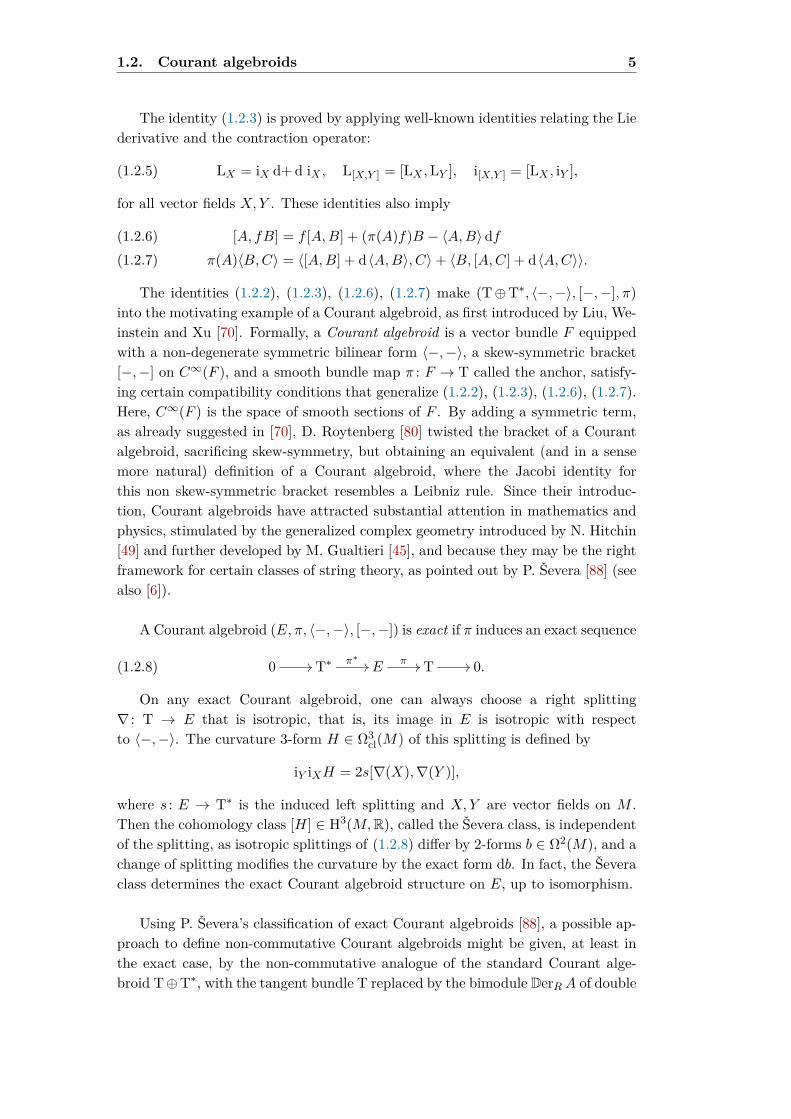
The identity (1.2.3) is proved by applying well-known identities relating the Liederivative and the contraction operator:
(1.2.5) LX = iX d+ d iX , L[X,Y ] = [LX ,LY ], i[X,Y ] = [LX , iY ],
for all vector fields X,Y . These identities also imply
[A, fB] = f [A,B] + (π(A)f)B − 〈A,B〉 df(1.2.6)π(A)〈B,C〉 = 〈[A,B] + d〈A,B〉, C〉+ 〈B, [A,C] + d〈A,C〉〉.(1.2.7)
The identities (1.2.2), (1.2.3), (1.2.6), (1.2.7) make (T⊕T∗, 〈−,−〉, [−,−], π)into the motivating example of a Courant algebroid, as first introduced by Liu, We-instein and Xu [70]. Formally, a Courant algebroid is a vector bundle F equippedwith a non-degenerate symmetric bilinear form 〈−,−〉, a skew-symmetric bracket[−,−] on C∞(F ), and a smooth bundle map π : F → T called the anchor, satisfy-ing certain compatibility conditions that generalize (1.2.2), (1.2.3), (1.2.6), (1.2.7).Here, C∞(F ) is the space of smooth sections of F . By adding a symmetric term,as already suggested in [70], D. Roytenberg [80] twisted the bracket of a Courantalgebroid, sacrificing skew-symmetry, but obtaining an equivalent (and in a sensemore natural) definition of a Courant algebroid, where the Jacobi identity forthis non skew-symmetric bracket resembles a Leibniz rule. Since their introduc-tion, Courant algebroids have attracted substantial attention in mathematics andphysics, stimulated by the generalized complex geometry introduced by N. Hitchin[49] and further developed by M. Gualtieri [45], and because they may be the rightframework for certain classes of string theory, as pointed out by P. Ševera [88] (seealso [6]).
A Courant algebroid (E, π, 〈−,−〉, [−,−]) is exact if π induces an exact sequence
(1.2.8) 0 // T∗ π∗ // Eπ // T // 0.
On any exact Courant algebroid, one can always choose a right splitting∇ : T → E that is isotropic, that is, its image in E is isotropic with respectto 〈−,−〉. The curvature 3-form H ∈ Ω3
cl(M) of this splitting is defined by
iY iXH = 2s[∇(X),∇(Y )],
where s : E → T∗ is the induced left splitting and X,Y are vector fields on M .Then the cohomology class [H] ∈ H3(M,R), called the Ševera class, is independentof the splitting, as isotropic splittings of (1.2.8) differ by 2-forms b ∈ Ω2(M), and achange of splitting modifies the curvature by the exact form db. In fact, the Ševeraclass determines the exact Courant algebroid structure on E, up to isomorphism.
Using P. Ševera’s classification of exact Courant algebroids [88], a possible ap-proach to define non-commutative Courant algebroids might be given, at least inthe exact case, by the non-commutative analogue of the standard Courant alge-broid T⊕T∗, with the tangent bundle T replaced by the bimodule DerRA of double

6 Introduction
derivations, and the cotangent bundle T∗ replaced by the bimodule Ω1RA of differ-
ential forms. Furthermore, one might define the Courant bracket combining thede Rham differential [31], certain non-commutative analogues of the Lie derivativeand the contraction operator of a double derivation with differential forms [30],and the double Schouten–Nijenhuis [96]. However, this direct attempt is not satis-factory because, to check the Kontsevich–Rosenberg principle in the representationspaces, we need non-commutative versions of the identities (1.2.5), that so far havenot been proved in this setting of non-commutative algebraic geometry.
1.3 Symplectic NQ-manifolds
An alternative approach to define non-commutative Courant algebroids is mo-tivated by graded geometry. An N-graded manifold (or N-manifold, for short)M of weight n and dimension (p; r1, ..., rn) is a smooth p-dimensional man-ifold M endowed with a sheaf C∞(M) of N-graded commutative associativeunital R-algebras, that is locally isomorphic to a (graded) polynomial ringC∞U (M)[ξ1
1 , . . . , ξr11 , ξ
12 , . . . , ξ
r22 , . . . , ξ
1n, . . . , ξ
rnn ], for open subsets U ⊂ M , where ξji
are variables of weight i (where the grading is called weight). The graded structureof C∞(M) determines a graded Euler vector field Eu on M, that acts on vectorfields and differential forms onM via the Lie derivative, whereby objects such assymplectic and Poisson structures also acquire weights. In particular, a symplecticstructure of weight n is a closed non-degenerate 2-form ω such that LEuω = nω.
Inspired by independent unpublished observations by Y. Kosmann-Schwarzbach, P. Ševera and P. Xu on the relationship of derived brackets withthe Courant brackets (see e.g. [61, §3.4]), and A. Yu. Vaintrob [94], who inter-preted Lie algebroids as odd self-commuting vector fields on a supermanifold, D.Roytenberg [81], following ideas of Ševera [88, 89], proved that Courant algebroidsare equivalent to symplectic NQ-manifolds of weight 2. Here, an NQ-manifold(M, Q) is an N-manifold M endowed with an integrable homological vector fieldQ of weight +1 (“homological” means [Q,Q] = 2Q2 = 0, where [−,−] is the gradedcommutator), and a symplectic NQ-manifold (M, ω,Q) is an NQ-manifold whosehomological vector field is compatible with a symplectic form ω, that is, LQω = 0,where LQ is the Lie derivative along the homological vector field Q.
Theorem 1.3.1 ([81], Theorem 3.3 & Theorem 4.5).
(i) Symplectic N-manifolds of weight 2 are in one-to-one correspondence withpseudo-Euclidean vector bundles.
(ii) Symplectic NQ-manifolds of weight 2 are in 1-1 correspondence with Courantalgebroids.
Symplectic NQ-manifolds are generalizations of PQ-manifolds on supermani-folds, introduced by A. Schwarz [85] as a geometric version of the formalism de-

1.4. Bi-symplectic NQ-algebras 7
veloped by I. Batalin and G. Vilkovisky [10] in physics to quantize classical fieldtheories in the Lagrangian formalism. Here, a P -structure is an odd-symplecticstructure and a Q-structure is a nilpotent vector field given by the odd-Poissonbracket with an action functional. From this view point, the N-grading can beviewed as an enhancement of the Z/2-grading to keep track of the ghost number.
We should also mention that D. Roytenberg [81] also classified NQ-manifolds ofweight 1. This result has applications in two-dimensional Topological Field Theory.
Theorem 1.3.2 ([81], Proposition 3.1 & Proposition 4.1).
(i) Symplectic N-manifolds of weight 1 are in 1-1 correspondence with ordinarysmooth manifolds. The correspondence attaches to each smooth manifold N ,the symplectic N-manifold (T∗[1]N,ω), where ω is determined by the Schoutenbracket of multivector fields.
(ii) Symplectic NQ-manifolds of weight 1 are in 1-1 correspondence with ordinaryPoisson manifolds.
1.4 Bi-symplectic NQ-algebras
Theorem 1.3.1 suggests a strategy to define non-commutative Courant algebroidssatisfying the Kontsevich–Rosenberg principle. Namely, in this thesis we will adaptD. Roytenberg’s constructions [81] — based on P. Ševera’s insights [88] — to a ver-sion of non-commutative algebraic geometry where the bi-symplectic structures [30]and the double Poisson structures [96] will be the main cornerstones replacing thecorresponding standard geometric structures. In this approach, our first aim is todefine suitable non-commutative analogues of symplectic NQ-manifolds.
A tensor N-algebra is an N-graded associative algebra that is the tensor al-gebra of a positively graded bimodule M , whose underlying ungraded bimoduleis projective and finitely generated over the weight-zero subalgebra A0 ⊂ A. Abi-symplectic NQ-algebra of weight N is a tensor N-algebra of weight N endowedwith a bi-symplectic form ω of weight N and a bi-symplectic double derivation Qof weight +1, with Q,Q = 0, where −,− is the canonical double Schouten–Nijenhuis bracket on double derivations. To construct these objects, we will needgeneralizations to graded associative algebras of tools introduced in [30, 31, 96] —these foundations are the contents of Chapter 2.
The next steps followed in this thesis to construct non-commutative Courantalgebroids will be, according to D. Roytenberg’s proof of Theorem 1.3.1, as follows:
(a) Start with a bi-symplectic NQ-algebra (A,ω,Q) of weight 2.
(b) Show that the underlying bi-symplectic tensor N-algebra A of weight 2 isdetermined by a pair (E, 〈−,−〉) consisting of a projective finitely generatedA0-bimodule E, endowed with a symmetric non-degenerate pairing 〈−,−〉.

8 Introduction
(c) Use the double derivation Q to determine a bracket [[ −,− ]] on E and ananchor ρ : E → DerR(A0).
(d) As a conclusion, from a bi-symplectic NQ-algebra of weight 2, construct anon-commutative Courant algebroid, defined a 4-tuple (E, 〈−,−〉, [[ −,− ]] , ρ).
To shorten notation, hereafter we define B = A0 — an ungraded subalgebra of A.
1.5 Bi-symplectic NQ-algebras of weight 1 and double Poissonalgebras
As in the case of manifolds, the classification of bi-symplectic NQ-algebras ofweight 1 provides a preliminary test to examine the tools introduced so far (thisclassification is carried out in Chapter 4), and furthermore, provides new insightsinto the structure of M. Van den Bergh’s double Poisson algebras.
Theorem 1.5.1 (Theorems 4.2.1 and 4.3.2).
(i) Bi-symplectic tensor smooth N-algebras of weight 1 are in 1-1 correspondence,up to isomorphism, with smooth associative R-algebras. The correspondenceassigns to each smooth associative R-algebra B, the pair (A,ω) consisting ofthe tensor N-algebra
A = T∗[1]B := TB(DerRB[−1])
and the bi-symplectic form ω determined by the double Schouten–Nijenhuisbracket of the tensor algebra of the B-bimodule of double derivations over B.
(ii) Bi-symplectic NQ-algebras of weight 1 are in 1-1 correspondence, up toisomorphism, with double Poisson algebras.
The main technical result used in the proof is a graded non-commutative versionin weight 0 of the Darboux theorem in symplectic geometry. As a similar result willbe needed for weight 2, we will show a more general result, valid for bi-symplectictensor N-algebras (A,ω) of arbitrary weight N over a smooth associative R-algebraB. By definition, A = TBM is a tensor algebra of a positively graded B-bimodule
M := M1 ⊕ · · · ⊕MN ,
where Mi = Ei[−i] ⊂ M is the homogeneous B-sub-bimodule of weight i, fori = 1, . . . , N . Here, V [−j]i := Vi−j for a graded vector space or (bi)module Vand j ∈ Z, so Ei are B-bimodules of weight 0 (see §2.1). As a bi-symplecticform ω ∈ DR2
R (A) has weight N , it determines an A-bimodule isomorphismι(ω) : DerRA
∼=−→ Ω1RA[−N ] (cf. (1.1.4)); in Theorem 3.2.2, we show that it
restricts to a B-bimodule isomorphism
(1.5.2) ι(ω)(0) : DerRB∼=−→ EN .

1.6. Bi-symplectic N-algebras of weight 2 9
1.6 Bi-symplectic N-algebras of weight 2
Our aim in Chapter 5 is to describe bi-symplectic tensor N-algebras (A,ω) of weight2 satisfying the above condition (a). On the one hand, by definition, A := TBM
with M := E1[−1] ⊕ E2[−2], for weight-zero B-bimodules E1 and E2, so A hasB-sub-bimodules of weights 0, 1, 2, given by
A0 = B, A1 = E1, A2 = (E1 ⊗B E1)⊕ E2,
and hence we have a trivial B-bimodule short exact sequence
0 // E1 ⊗B E1 // A2 // E2 // 0.
On the other hand, the bi-symplectic form ω ∈ DR2R (A) of weight 2 induces
a double Poisson bracket −,−ω of weight -2, providing a family of doublederivations and a family of double differential operators defined, respectively, as
X : A2 −→ DerRB : a 7−→ (Xa := a,−ω |B : B −→ B)D : A2 −→ EndRe(E1) : a 7−→ (Da := a,−ω |E1 : E1 7−→ E1 ⊗B ⊕B ⊗ E1) ,
where EndRe(E1) := HomRe(E1, E1 ⊗B ⊕B ⊗ E1).
Furthermore, −,−ω restricts to a pairing 〈−,−〉 on E1 (in the sense of M.Van den Bergh [97]), that is symmetric in the sense that 〈e1, e2〉 = 〈e2, e1〉 forall e1, e2 ∈ E1. Following D. Roytenberg’s method, we need to show this pair-ing is non-degenerate (i.e. it induces an isomorphism between E1 and its bidualE∨1 := HomBe(E1,BeBe)). This result is achieved using a Darboux-type theoremin weight 1, obtained in the framework of double graded quivers, whose basic struc-ture is explained in §3.3.1. A double graded quiver P is obtained from a gradedquiver P of weight |P | = N by adjoining a reverse arrow a∗ : j → i for each arrowa : i → j in P and whose weight is |a∗| = N − |a| (see Definition 3.3.4). To adouble graded quiver P (of even weight N), we can attach a bi-symplectic tensorN-algebra A of weight N , defined simply as the graded path algebra of P , with thebi-symplectic form ω =
∑a∈P1
dada∗ of weight N . In this case, A0 = B is the pathalgebra of the weight 0 subquiver of P . In Theorem 3.3.40, we prove that whenN = 2, the isomorphism ι(ω) restricts, in weight 1, to an isomorphism [ : E1 → E∨1 .This map enables us to define a symmetric non-degenerate pairing 〈−,−〉 on E1,that coincides with the restriction −,−ω |E1⊗E1 : E1 ⊗ E1 → B ⊗B.
Using the pair (E1, 〈−,−〉), we can construct a non-commutative analogueAt(E1) of the Atiyah algebroid, called the metric double Atiyah algebra, definedas the space consisting of pairs (X,D) with X ∈ DerRB,D ∈ EndRe(E1), such that
D(be) = bD(e) + X(b)e, D(eb) = D(e)b+ eX(b),
for all b ∈ B, e ∈ E, and which, in addition, preserve the pairing 〈−,−〉, that is,
σ(123)X(〈e2, e1〉) = 〈e1,D(e2)〉L + σ(132)〈e2,D(e1)〉L,
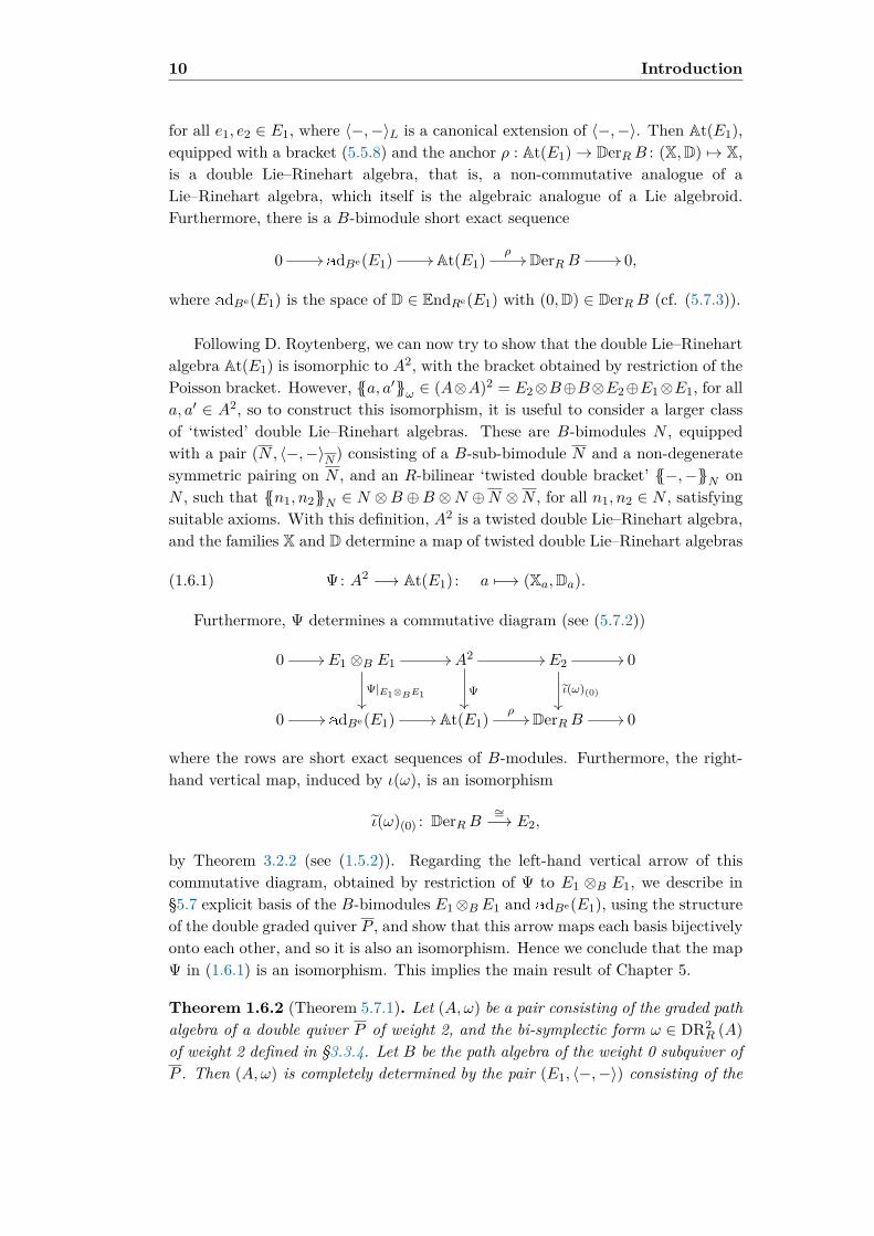
10 Introduction
for all e1, e2 ∈ E1, where 〈−,−〉L is a canonical extension of 〈−,−〉. Then At(E1),equipped with a bracket (5.5.8) and the anchor ρ : At(E1)→ DerRB : (X,D) 7→ X,is a double Lie–Rinehart algebra, that is, a non-commutative analogue of aLie–Rinehart algebra, which itself is the algebraic analogue of a Lie algebroid.Furthermore, there is a B-bimodule short exact sequence
0 //adBe(E1) // At(E1) ρ
// DerRB // 0,
where adBe(E1) is the space of D ∈ EndRe(E1) with (0,D) ∈ DerRB (cf. (5.7.3)).
Following D. Roytenberg, we can now try to show that the double Lie–Rinehartalgebra At(E1) is isomorphic to A2, with the bracket obtained by restriction of thePoisson bracket. However, a, a′ω ∈ (A⊗A)2 = E2⊗B⊕B⊗E2⊕E1⊗E1, for alla, a′ ∈ A2, so to construct this isomorphism, it is useful to consider a larger classof ‘twisted’ double Lie–Rinehart algebras. These are B-bimodules N , equippedwith a pair (N, 〈−,−〉N ) consisting of a B-sub-bimodule N and a non-degeneratesymmetric pairing on N , and an R-bilinear ‘twisted double bracket’ −,−N onN , such that n1, n2N ∈ N ⊗B ⊕B ⊗N ⊕N ⊗N , for all n1, n2 ∈ N , satisfyingsuitable axioms. With this definition, A2 is a twisted double Lie–Rinehart algebra,and the families X and D determine a map of twisted double Lie–Rinehart algebras
(1.6.1) Ψ: A2 −→ At(E1) : a 7−→ (Xa,Da).
Furthermore, Ψ determines a commutative diagram (see (5.7.2))
0 // E1 ⊗B E1 //
Ψ|E1⊗BE1
A2 //
Ψ
E2 //
ι(ω)(0)
0
0 //adBe(E1) // At(E1) ρ
// DerRB // 0
where the rows are short exact sequences of B-modules. Furthermore, the right-hand vertical map, induced by ι(ω), is an isomorphism
ι(ω)(0) : DerRB∼=−→ E2,
by Theorem 3.2.2 (see (1.5.2)). Regarding the left-hand vertical arrow of thiscommutative diagram, obtained by restriction of Ψ to E1 ⊗B E1, we describe in§5.7 explicit basis of the B-bimodules E1⊗B E1 and adBe(E1), using the structureof the double graded quiver P , and show that this arrow maps each basis bijectivelyonto each other, and so it is also an isomorphism. Hence we conclude that the mapΨ in (1.6.1) is an isomorphism. This implies the main result of Chapter 5.
Theorem 1.6.2 (Theorem 5.7.1). Let (A,ω) be a pair consisting of the graded pathalgebra of a double quiver P of weight 2, and the bi-symplectic form ω ∈ DR2
R (A)of weight 2 defined in §3.3.4. Let B be the path algebra of the weight 0 subquiver ofP . Then (A,ω) is completely determined by the pair (E1, 〈−,−〉) consisting of the

1.7. Bi-symplectic NQ-algebras of weight 2 and doubleCourant–Dorfman algebras 11
B-bimodule E1, with basis consisting of weight 1 paths in P , and the symmetricnon-degenerate pairing
〈−,−〉 := −,−ω |E1⊗E1 −→ B ⊗B.
1.7 Bi-symplectic NQ-algebras of weight 2 and double Courant–Dorfman algebras
In Chapter 6, we focus on the construction of non-commutative Courant algebroids,using the pairs (E1, 〈−,−〉) of Theorem 1.6.2. More precisely, a double pre-Courant–Dorfman algebra over the R-algebra B is a 4-tuple (E, 〈−,−〉, ρ, [[ −,− ]] )consisting of a projective finitely generated B-bimodule E endowed with asymmetric non-degenerate pairing (the inner product)
〈−,−〉 : E ⊗ E −→ B ⊗B,
a B-bimodule morphism
(1.7.1) ρ : E −→ DerRB,
called the anchor, and an operation
(1.7.2) [[ −,− ]] : E ⊗ E −→ (E ⊗B)⊕ (B ⊗ E),
called the double Dorfman bracket, which is R-linear for the left Be-module struc-ture on Be in the second argument and R-linear for the right Be-module struc-ture on Be in the first argument. These data must satisfy certain compatibilityconditions (see (6.3.4) in Definition 6.3.1). In addition, if the double pre-Courant–Dorfman algebra satisfies the “double Jacobi–Courant rule” (6.3.5), the 4-tuple(E, 〈−,−〉, ρ, [[ −,− ]] ) is called a double Courant–Dorfman algebra.
As in the commutative case, given a bi-symplectic NQ-algebra (A,ω,Q) ofweight 2, the homological double derivation can be written as Q = S,−ω, whereS ∈ A3 enables us to recover the structure of double pre-Courant–Dorfman algebrausing derived brackets in this framework (see Proposition 6.4.2) by the formulae
ρ(e1)(b) := S, e1ω, bω ,[[ e1, e2 ]] := S, e1ω, e2ω ,
for all b ∈ B and e1, e2 ∈ E1, where −,−ω = m −,−ω is the associatedbracket in A (see (2.3.5)). Then the condition Q,Q = 0 implies S, Sω = 0,whereas the latter condition implies the “double Jacobi–Courant identity” in(6.3.5), by Proposition 6.4.6, so we obtain a double Courant–Dorfman algebra(E1, 〈−,−〉, ρ, [[ −,− ]] ).
In conclusion, we obtain the main result of this thesis:

12 Introduction
Theorem 1.7.3 (Theorem 6.4.8). Let (A,ω,Q) be a bi-symplectic NQ-algebra ofweight 2, where A is the graded path algebra of a double quiver P of weight 2 en-dowed with a bi-symplectic form ω ∈ DR2
R (A) of weight 2 defined in §3.3.4 anda homological double derivation Q. Let B be the path algebra of the weight 0 sub-quiver of P , and (E1, 〈−,−〉) the pair consisting of the B-bimodule E1 with basisconsisting of the weight 1 paths in P and the symmetric non-degenerate pairing〈−,−〉 := −,−ω |E1⊗E1 → B ⊗B.
Then the triple (A,ω,Q) determines an element S ∈ A3 such that
(i) S induces a double pre-Courant–Dorfman algebra structure on (E1, 〈−,−〉)by
ρ(e1)(b) := S, e1ω, bω , [[ e1, e2 ]] := S, e1ω, e2ω ,
for all b ∈ B, e1, e2 ∈ E1, where −,−ω = m −,−ω is the associatedbracket in A.
(ii) The bi-symplectic NQ-algebra (A,ω,Q) of weight 2 induces a double Courant–Dorfman algebra (E1, 〈−,−〉, ρ, [[ −,− ]] ) over B.
1.8 Contents of the thesis
In Chapter 2, we introduce graded versions of basics notions defined in non-commutative symplectic geometry by Crawley-Boevey, Etingof and Ginzburg [30],and in non-commutative Poisson geometry by Van den Bergh [96]. To fix nota-tion, in §2.1 we start reviewing graded versions of well-known constructions forbasic objects, such as algebras and modules, and above all, we introduce the outerand inner bimodule structures on A ⊗ A, for a graded algebra A (see (2.1.21)).In §2.1.2 we present some classical results concerning isomorphisms of (projec-tive finitely generated) graded A-modules. Adapting constructions of Cuntz andQuillen [31] and Crawley-Boevey, Etingof and Ginzburg [30] to a graded algebraA over an associative algebra R, in §2.2 we define the bimodules Ω1
RA and DerRAof non-commutative relative differentials forms and double derivations §2.2.4, andthe notion of smoothness for A over R (see Definition 2.2.22). In this thesis, thekey example of a smooth algebra will be the tensor algebra satisfying suitable con-ditions specified in Proposition 2.2.23.
After the preliminary definitions and facts included in §2.1, §2.1.2, in §2.3–§2.5we introduce graded versions of basic concepts in non-commutative Poisson andsymplectic structures. First, in §2.3.1, we review Van den Bergh’s double Pois-son algebras [96], and define double Poisson graded algebras (see Definition 2.3.9).Then we define the graded double Schouten–Nijenhuis bracket (see (2.3.14)), reviewbi-symplectic forms and Hamiltonian double derivations (see Definition 2.4.1), in-troduce bi-symplectic associative graded algebras (Definition 2.5.3) and prove somebasic results about them (Lemma 2.5.5 and 2.5.6). Finally, in §2.6, we review how

1.8. Contents of the thesis 13
the Kontsevich–Rosenberg principle works for bi-symplectic forms.
In Chapter 3 we shall prove two technical results of graded bi-symplectic forms,roughly speaking corresponding to graded non-commutative versions, in weights 1and 2, of the Darboux Theorem in symplectic geometry (as explained, for in-stance, in [18], §8.1). They turn out to be essential in subsequent chapters. In§3.1, following [31], we introduce the cotangent exact sequence relating absoluteand relative differential forms, and also study its bidual (see Lemma 3.1.10). In§3.2, we introduce the crucial notion of bi-symplectic tensor N-algebra of weight N(here N ∈ N∗) which, in particular establishes an isomorphism between the spaceof double derivations and the bimodule of non-commutative differential 1-formson the tensor N-algebra given by ω, the bi-symplectic form of weight N . Thefirst technical result is Theorem 3.2.2. It states that if (A,ω), with A = TB is abi-symplectic tensor N-algebra of weight N where R is a semisimple finite dimen-sional k-algebra, B is a smooth R-algebra and M := E1[−1] ⊕ · · · ⊕ EN [−N ] forfinitely generated projective B-bimodules Ei for all 1 ≤ i ≤ N , the isomorphismι(ω) : DerRA −→ Ω1
RA[−N ] restricts, in weight 0, to the B-bimodule isomorphismι(ω)(0) : DerRB
∼=−→ EN .
The second technical result is Theorem 3.3.40 where we carry out the con-struction of the isomorphism [ : E1 → E∨1 which turns out to be the restrictionof the isomorphism ι(ω) in weight 1. This Theorem is proved in the setting ofgraded double quivers (of weight 2) whose basics are reviewed in §3.3.1 (see Defi-nition 3.3.4). In particular, since the graded path algebra of these objects can beexpressed in terms of the graded tensor algebra of the bimodule VP and as thegraded tensor of the bimodule MP (see (3.3.5) and (3.3.25)), in Lemma 3.3.7 weprove that there exists a canonical isomorphism between both descriptions. Fi-nally, in Proposition 3.3.34, we show that graded double quivers are endowed witha canonical bi-symplectic form of even weight.
D. Roytenberg [81] proved that symplectic NQ-manifolds of weight 1 are in 1-1correspondence with ordinary Poisson manifolds. In Chapter 3, we extend this re-sult to the noncommutative setting using techniques of noncommutative algebraicgeometry.
Once we review Roytenberg’s result in §4.1, we carry out the classification ofbi-symplectic tensor N-algebras of weight 1 (see §4.2), which are in 1-1 correspon-dence with smooth associative algebras. In the last section of the chapter, weintroduce the essential notion of bi-symplectic NQ-algebras (which can be regardedas the noncommutative analogues of symplectic NQ-manifolds) and in Theorem4.3.2 we classify them in weight 1: bi-symplectic NQ-algebras of weight 1 are in1-1 correspondence with double Poisson algebras.
Chapter 5 is somehow the core of this thesis. In §5.1 we sketch a result of

14 Introduction
D. Roytenberg that can be reformulated more algebraically using Lie–Rinehartalgebras (the algebraic structure corresponding to Lie algebroids) as follows: thestructure of a symplectic polynomial N-algebra of weight 2 is completely deter-mined by a finitely generated projective B-module E1 endowed with a symmetricnon-degenerate bilinear form 〈−,−〉 (see [81], Theorem 3.3). In §5.2, if B is asmooth associative algebra, given a bi-symplectic tensor N-algebra of weight 2 overB A = TB(E1[−1] ⊕ E2[−2] where E1 and E2 are projective finitely generatedB-bimodules, we calculate A0, A1 and A2, the subspaces Aw ⊂ A of weights 0,1,2,and determine the structure of the double Poisson bracket of weight -2 induced bythe bi-symplectic form. §5.4 is devoted to define a non-commutative counterpartof a Lie–Rinehart algebra (see Definition 5.4.1) and to prove in Proposition 5.4.9that A2 has this structure.
A key point in our discussion is that E1 is endowed with a pairing (in the senseof [97], §3.1), whose definition is reviewed in (5.3.3). Using the results of §3.3,we construct a non-degenerate symmetric pairing for double graded quivers (seeLemma 5.3.7). In §5.3.4, we prove that this pairing is compatible, in a suitablesense (see §5.3.4), with certain family of “double covariant differential operators”Da introduced in §5.3.2.
In §5.5 we introduce the notion of double Atiyah algebra and metric doubleAtiyah algebra At(E1) which are endowed with brackets (5.5.8), resembling Vanden Bergh’s double Schouten–Nijenhuis bracket. In Proposition 5.5.10 we provethat At(E1) is a double Lie–Rinehart algebra. Finally, §5.6 is devoted to prove thata map Ψ: A2 → At(E1), defined in (5.6.2) using the “double covariant differen-tial operators”, is a map of twisted double Lie–Rinehart algebras (see Proposition5.6.1). Furthermore, in §5.7 we demonstrate that, in the setting of double gradedquivers, Ψ is an isomorphism and, consequently, we conclude that our bi-symplectictensor N-algebra A over B of weight 2 is completely determined by E1 togetherwith its non-degenerate symmetric pairing.
In Chapter 6, we calculate the non-commutative structures that arise when weequip a graded bi-symplectic tensor algebra (A,ω) of weight 2 with a homologicaldouble derivation Q. Here, a double derivation Q on A is homological if it satisfiesthe “double Maurer–Cartan” equation Q,Q = 0, where −,− is the doubleSchouten–Nijenhuis commutator. Since our calculations will be based on results ofChapter 4, we focus on the case where (A,ω) is a bi-symplectic graded path algebraof a double graded quiver (see (3.3.4)). The new algebraic structures will be called“double Courant–Dorfman algebras”. They are non-commutative versions of theCourant–Dorfman algebras introduced by Roytenberg [83], that themselves are toCourant algebroids what Lie–Rinehart algebras are to Lie algebroids.
In §6.1, we start with a short review of the role of Courant algebroids in ge-ometry and physics (§6.1.1) and their definition §6.1.2. In §6.2 we provide an

1.8. Contents of the thesis 15
algebraic reformulation of Roytenberg’s correspondence between symplectic NQ-manifolds of weight 2 and Courant algebroids. Finally, in §6.3.1 we define thecentral object of this chapter –double Courant–Dorfman algebras–, and show thata bi-symplectic NQ-algebra (A,ω) attached to a double graded quiver P determinesa double Courant–Dorfman algebra over the path algebra of the weight 0 subquiverQ of P .
Finally, in Chapter 7, we present some questions and open directions which thisthesis gives rise.


Chapter 2
Basics on (graded) non-commutativealgebraic geometry
In this chapter, we introduce graded versions of basics notions defined in non-commutative symplectic geometry by Crawley-Boevey, Etingof and Ginzburg [30],and in non-commutative Poisson geometry by Van den Bergh [96]. To fix nota-tion, in §2.1 we start reviewing graded versions of well-known constructions forbasic objects, such as algebras and modules, and above all, we introduce the outerand inner bimodule structures on A ⊗ A, for a graded algebra A (see (2.1.21)).In §2.1.2 we present some classical results concerning isomorphisms of (projec-tive finitely generated) graded A-modules. Adapting constructions of Cuntz andQuillen [31] and Crawley-Boevey, Etingof and Ginzburg [30] to a graded algebraA over an associative algebra R, in §2.2 we define the bimodules Ω1
RA and DerRAof non-commutative relative differentials forms and double derivations §2.2.4, andthe notion of smoothness for A over R (see Definition 2.2.22). In this thesis, thekey example of a smooth algebra will be the tensor algebra satisfying appropriateconditions specified in Proposition 2.2.23.
After the preliminary definitions and facts included in §2.1, in §2.2–§2.5 weintroduce graded versions of basic concepts in non-commutative Poisson andsymplectic structures. First, in §2.3.1, we review Van den Bergh’s double Poissonalgebras [96], and define double Poisson graded algebras (see Definition 2.3.9).Then we define the graded double Schouten–Nijenhuis bracket (see (2.3.14)), reviewbi-symplectic forms and Hamiltonian double derivations (see Definition 2.4.1),introduce bi-symplectic associative graded algebras (Definition 2.5.3) and provesome basic results about them (Lemma 2.5.5 and 2.5.6). Finally, in §2.6, weillustrate how the Kontsevich–Rosenberg principle works in some cases, includingbi-symplectic forms.
17

18 Basics on (graded) non-commutative algebraic geometry
2.1 Background on graded algebras and graded mod-ules
Notation and conventions
We will work over a fixed (commutative) base field k. From now on, all unadornedtensor products are over the base field k. We denote by Z the set of integers,by N = 0, 1, 2, ... the set of natural numbers, which by convention are the non-negative integers and by N∗ = 1, 2, 3, ... ⊂ N the set of positive integers. Finally,if V and W are k-vector spaces, then an element h ∈ V ⊗W is written as h′ ⊗ h′′.This is a shorthand for
∑i h′i ⊗ h′′i . From now on, we will use Sweedler’s notation
in a systematic way which consists of dropping the summation sign.
Graded vector spaces
Following [20] by a Z-graded vector space (or simply, a graded vector space) wemean a direct sum V =
⊕i∈Z Vi of vector spaces over the field k. The Vi are
called the components of V of degree i. An element v ∈ V is called homogeneousif v ∈ Vi for some i, and homogeneous of degree i if v ∈ Vi. Finally, the degree of ahomogeneous element v ∈ V to be denoted by |v|. Moreover, we also denote by V [n]the graded vector space with degree shifted by n, namely, V [n] =
⊕i∈Z(V [n])i with
V [n]i = Vi+n. If f : V → W is a map of graded vector spaces with homogeneouscomponents fl : Vi → Wj then let f [d] : V [d] → W [d] be the map of gradedvector spaces with homogeneous components f [d]l : V [d]i → W [d]j defined byf [d]l(v) = (−1)dfl+d(v) for v ∈ V [d]i = Vi+d.
Graded rings
We say that a ring R is Z-graded if there exists a family of subgroups Rnn∈Zof R such that R =
⊕n∈ZRn as abelian groups, and Rn · Rm ⊂ Rn+m for all
homogeneous n,m ∈ Z. Observe that if R =⊕
n∈ZRn is a graded ring, then R0is a subring of R, 1 ∈ R0 and Rn is an R0-module for all n. From now on, allrings will be associative with 1. Let S be a graded ring. A map f : R → S iscalled a graded ring homomorphism if f is a ring homomorphism, f(1R) = 1S andf respects the grading, that is, f(Rn) ⊂ Sn for each n.
Graded (associative) algebras
An associative graded k-algebra A (for short, a graded k-algebra, graded algebraover k or, simply, a graded algebra) is a a graded ring A together with a morphismk → A (called the structure map) into its graded centre, Z(A) whose definition is(see [65], p. 84) z ∈ A | za = (−1)|a||z|az for all homogeneous a ∈ A. A mor-phism of graded algebras is a morphism of graded rings that forms a commutativetriangle with the structure maps over k. In a parallel way, if R is an associativeunital k-algebra, we may develop the theory in the case of graded R-algebras, that

2.1. Background on graded algebras and graded modules 19
is, graded algebras endowed with an algebra homomorphism B → A compatiblewith the identity map R→ R (in particular, it is unit preserving).
Tensor product of graded algebras
In this subsection, we fix two graded algebras: A and B. Their tensor product isthe graded algebra with underlying graded vector space A⊗B, and multiplicationgiven by
(2.1.1) (a⊗ b)(a′ ⊗ b′) = (−1)|b||a′|aa′ ⊗ bb′.
The graded opposite algebra Aop is the graded algebra with the same underlyinggraded vector space as A and product given by
(2.1.2) aopbop := (−1)|a||b|(ba)op,
for homogeneous a, b ∈ A, where the symbol (−)op is used to distinguish themultiplication rules in A and Aop. Then there exist natural isomorphisms
(2.1.3) (Aop)op ' A, (A⊗B)op ' Aop ⊗Bop.
The graded enveloping algebra of A is the graded algebra
(2.1.4) Ae = A⊗Aop.
Hence the multiplication in Ae is given by
(a1 ⊗ bop1 )(a2 ⊗ bop
2 ) = (−1)|b1||a2|(a1a2)⊗ (bop1 b
op2 )
= (−1)|b1||a2|+|b1||b2|(a1a2)⊗ (b2b1)op,
for homogeneous ai ∈ A and bopi ∈ Aop with i = 1, 2. Then there exists a natural
isomorphism of graded algebras
(2.1.5)τ : Ae −→ (Ae)op
a1 ⊗ aop2 7−→ (−1)|a1||a2|(a2 ⊗ aop
1 )op,
with inverse
(2.1.6)τ−1 : (Ae)op −→ Ae
(a2 ⊗ aop1 )op 7−→ (−1)|a1||a2|a1 ⊗ aop
2 .
It is not difficult to check that, with this definition, τ is a morphism of gradedalgebras.

20 Basics on (graded) non-commutative algebraic geometry
Modules over graded algebras
Throughout, a graded A-module will be a graded left A-module M , that is, a gradedvector spaceM endowed with a multiplication map µM : A⊗M →M : a⊗m 7→ am,of degree zero, such that the diagrams
A⊗A⊗M µA⊗1//
1⊗µM
A⊗Mµ
A⊗M µ//M
k ⊗M //
IA⊗1A
M
A⊗M µM //M
commute.
Given two graded A-modules M and N , an A-module homomorphism f : N →M of degree d is a homomorphism of k-modules, f : Ni → Mj such that j = i+ d
and f(λn) = (−1)|f ||λ|λf(n) for all λ ∈ k, n ∈ N . The set of all such f is ak-module which we denote by Homd
A(N,M) and consider
Hom•A(N,M) :=⊕d∈Z
HomdA(N,M) =
⊕d∈Z
⊕j=i+d
hom(Ni,Mj),
where hom(−,−) is the functor between (ungraded) A-modules. To shortennotation, we shall make the identification HomA(−,−) := Hom•A(−,−) for a gradedalgebra A; this should no cause confusion by the context. In general, HomA(N,M)does not have a graded A-module structure. However, HomA(M,N) has a structureof Z(A)-module by defining
(z · f)(m) := z(f(m)).
A graded right A-module M is defined as a graded Aop-module. A graded(A,B)-bimodule is a graded (A⊗Bop)-module and a graded A-bimodule is a graded(A,A)-bimodule, i.e. a graded Ae-module. The multiplication map of a rightgraded A-module M will often be denoted M ⊗ A → M : m ⊗ a 7→ ma withma := (−1)|a||m|aopm. This definition insures that aop
1 (aop2 m) = (aop
1 aop2 )m.
Graded bimodules of various types can be described in terms of variouscompatible graded module structures. For instance, a graded (A,B)-bimodulestructure on M is equivalent to a graded left A-module structure and a gradedright B-module structure on M , such that the operators of A and B commute, i.e.(am)b = a(mb), where the (graded) A-module multiplication A⊗M →M : a⊗m 7→am and the (graded) B-module multiplication M ⊗ B → M : m ⊗ b 7→ mb arerespectively given by
am := (a⊗ 1opB )m,(2.1.7a)
mb := (−1)|m||b|(1A ⊗ bop)m.(2.1.7b)
The fact that these module commute means that a(mb) = (am)b, that is,(−1)|m||b|(a⊗ 1op
B )(1A ⊗ bop)m = (−1)(|a||b|+|m||b|)(1A ⊗ bop)(a⊗ 1opB )m.

2.1. Background on graded algebras and graded modules 21
Hence, in particular, for B = A, a graded Ae-module M can be described bya pair of commuting graded left and right A-module structures, respectively givenby
am := (a⊗ 1opA )m,(2.1.8a)
ma := (−1)|m||b|(1A ⊗ aop)m.(2.1.8b)
Similarly, a graded (A ⊗ B)-module structure on M is equivalent to a gradedA-module structure and a graded B-module structure on M , such that the opera-tors of A and B commute, that is, a(bm) = b(am), with multiplication maps givenby am := (a⊗ 1B)m and bm := (−1)|b||m|(1A ⊗ b)m.
We shall change between the above equivalent descriptions of graded left/rightmodules and bimodules when it is convenient; this should no cause confusion, as(Aop)op = A. Symbols such as AM , MA, A,BM , AMB or MA,B will indicate thatM is a graded (left) A-module, a graded right A-module, a graded (A⊗B)-module,a graded (A,B)-bimodule, or a graded right (A⊗B)-module, respectively.
Graded modules as representations
It is sometimes convenient to identify the category of graded A-modules with thecategory of representations of the graded algebra A. Consider the space of gradedendomorphisms
End•M =⊕l∈Z
EndlM =⊕l∈Z
⊕j=i+l
HomA(Mi,Mj),
on a graded vector space M , with HomA(−,−) denoting the A-module of (un-graded) homomorphisms. The multiplication of two such homogeneous mapsf1, f2 : M• →M• is provided by the composition (from right to left and with the ob-vious compatibility between the involved degrees) f2f1 : M →M to be a homoge-neous element of degree |f1|+|f2|. Again, to shorten notation, End(−) := End•(−)
A graded representation of A is a (unital) morphism of graded algebras ρ : A→EndM into the graded algebra. A morphism between graded representations,namely f : ρ1 → ρ2 is a graded linear map f : M• → M ′• such that for every i
and j the diagram
(2.1.9) Mifi //
ρ1(a)
M ′i
ρ2(a)
Mjfj//M ′j
commutes for all homogeneous a ∈ A. We will often identify graded A-modulesand graded A-representations using the isomorphism between their categories thatto each graded A-module M assigns the representation
ρM : A −→ EndM

22 Basics on (graded) non-commutative algebraic geometry
given by ρM (a)m := am, and to each representation ρ : A → EndM assigns thegraded A-module M with multiplication given by am := ρ(a)m.
Right Ae-modules as A-bimodules
The category of graded right Ae-modules is isomorphic to the category of gradedA-bimodules. To show this, it is more convenient to construct the correspondingisomorphism between the category of graded representations of (Ae)op and Ae. Theisomorphism assigns to each graded (Ae)op-representation ρ : (Ae)op → EndM , itscomposite
τ∗ρ := ρ τ : Ae −→ EndM,
with the graded algebra morphism τ in (2.1.5), and to each morphism f : ρ1 → ρ2 ofgraded (Ae)op-representations ρi : (Ae)op → EndMi, the same (graded) morphismf , regarded as a morphism τ∗f : τ∗ρ1 → τ∗ρ2 of graded (Ae)op-representations (thefact that f is a morphism of graded representations of Ae follows because if thediagram (2.1.9) commutes with a replaced by u, for all homogeneous u ∈ (Ae)op,then this diagram also commutes with a replaced by τ(u), for all homogeneousu ∈ Ae).
In the language of graded modules, this isomorphism assigns to each gradedright Ae-module M , the graded A-bimodule τ∗M with underlying graded vectorspace M and multiplication
(2.1.10) Ae ⊗ τ∗M −→ τ∗M : (a1 ⊗ aop2 )⊗m 7−→ (a1 ⊗ aop
2 ) ∗m
given by
(2.1.11) (a1 ⊗ aop2 ) ∗m := τ(a1 ⊗ aop
2 )m = (−1)|a1||a2|(a2 ⊗ aop1 )opm.
As in (2.1.8), this latter graded A-bimodules structure can be described in terms ofa pair of commuting graded left and right A-module structures, respectively givenby
a1 ∗m := (a1 ⊗ 1opA ) ∗m = (1A ⊗ aop
1 )opm,(2.1.12a)
m ∗ a2 := (−1)|a2||m|(1A ⊗ aop2 ) ∗m = (−1)|a2||m|(a2 ⊗ 1op
A )opm.(2.1.12b)
We will often identify a graded right Ae-module M with the corresponding Ae-module τ∗M , dropping the symbol τ∗, and distinguish them with the lower indicesMAe and AeM , respectively. Finally, observe that for any graded right Ae-moduleM , its underlying ungraded right Ae-module is finitely generated and projective ifand only if the underlying ungraded corresponding to τ∗M so is.
Transference of operators
When two graded modules have some extra operators, it is possible to transferthem to their graded tensor product or to the space of graded homomorphisms

2.1. Background on graded algebras and graded modules 23
(when these spaces are defined). As usual, let A and B be graded algebras. Then,recall that HomA(M,N) is defined whenM and N be both graded (left) A-moduleswhile the graded tensor product M ⊗A N is defined when M is a right graded A-module and N is a left graded A-module.
For instance, for a graded (A,B)-bimodule M and a graded A-module N , thespace HomA(M,N) of graded A-module homomorphisms is a graded (left) B-module, with multiplication B ⊗HomA(M,N)→ HomA(M,N) given by
(2.1.13) (bf)(m) := (−1)|f ||b|f(mb).
It is straightforward to check the associativity property. Similarly, for a graded A-module M and a graded (A,B)-bimodule N , the space HomA(M,N) is a gradedright B-module, with multiplication given by
(2.1.14) (fb)(m) = f(m)b.
Moreover, for a graded (A,B)-bimodule M and a graded B-module N , thegraded tensor product M ⊗B N over B is graded A-module, with multiplicationmap A⊗ (M ⊗B N)→M ⊗B N given by
(2.1.15) a(m⊗ n) = (am)⊗ n,
for homogeneous a ∈ A, m ∈M , n ∈ N .
If the graded homomorphisms or graded tensor products are ‘external’, i.e.defined over the base field rather than a graded algebra, it is possible to transferall the operators in a compatible way. For example, for a graded A-module M anda graded B-module N , the space Hom(M,N) of k-linear graded maps f : M• → N•is a graded (B,A)-bimodule, with multiplication
(2.1.16) ((b⊗ aop)f)(m) = (bfa)(m) := (−1)|f ||a|b(f(am)),
for homogeneous a ∈ A, b ∈ B, m ∈ M , whereas for a graded right A-module Mand a graded right B-module N , the space Hom(M,N) of graded k-linear mapsf : M → N is a graded (A,B)-bimodule, with multiplication
(2.1.17) ((a⊗ bop)f) (m) = (afb)(m) := (−1)|f |(|a|+|b|)f(ma)b.
Similarly, for a graded right A-moduleM and a graded B-module N , the spaceHom(M,N) of k-linear maps f : M → N is a a graded (A ⊗ B)-module, withmultiplication given by
(2.1.18) ((a⊗ b)f)(m) = (−1)|f |(|a|+|b|)bf(ma).
Finally, as a final example, the graded tensor product M ⊗ N over the basefield k is a graded (A⊗B)-module, with multiplication given by
(2.1.19) (a⊗ b)(m⊗ n) := (−1)|b||m|(am)⊗ (bn).

24 Basics on (graded) non-commutative algebraic geometry
Graded modules underlying a graded algebra
The underlying graded vector space of a graded algebra A is automatically a gradedAe-module, denoted AeA, with multiplication given by
(a⊗ bop)m = (−1)|m||b|amb,
for homogeneous a ⊗ bop ∈ Ae, m ∈ AeA or, in other words, a graded A-bimodule, denoted AAA, with the left and right multiplications am and ma givenby multiplication in A, for homogeneous a ∈ A and m ∈ AAA. Then AA and AArespectively denote the graded left and right A-modules with underlying gradedvector space A, with the graded A-module structures respectively given by left andright multiplications.
2.1.1 Outer and inner bimodule structures
By the construction discussed in the previous subsection, the underlying gradedvector space of Ae becomes a graded (Ae)e-module (Ae)e(Ae), with multiplication
((a1 ⊗ bop1 )⊗ (a2 ⊗ bop
2 )op) (a⊗ bop) = ±((a1aa2)⊗ (b2bb1)op)
for homogeneous (a1 ⊗ bop1 ) ⊗ (a2 ⊗ bop
2 )op ∈ (Ae)e, a ⊗ bop ∈ (Ae)e(Ae) and where± = (−1)(|a2||a|+|b||b1|+|b1||a2|+|b1||b2|). Moreover, by the equivalent descriptions of§2.1, this graded Ae-bimodule Ae(Ae)Ae = (Ae)e(Ae) corresponds to a pair of com-muting graded left and right Ae-module structures on Ae.
Let (A ⊗ A)out be the graded A-bimodule corresponding to the graded leftAe-module structure Ae(Ae), and (A⊗A)inn the A-bimodule corresponding to thegraded right Ae-module structure (Ae)op(Ae) = (Ae)Ae via (2.1.11) and (2.1.12)applied to M = (Ae)op(Ae). In other words,
(2.1.20) (A⊗A)out := AeAe, (A⊗A)inn := τ∗(AeAe).
In the second identity, we will often drop the symbol τ∗ and use the symbol AeAe
to indicate the graded right Ae-module structure. By (2.1.8), (2.1.11) and (2.1.12)applied to m = a⊗ b, these graded bimodule structures are given by
a1(a⊗ b)b1 = (−1)(|a|+|b|)|b1|(a1 ⊗ bop1 )(a⊗ bop)
= (−1)|b||b1|(a1a)⊗ (bop1 b
op)= (a1a)⊗ (bb1) in (A⊗A)out,
On the other hand, by (2.1.11),
b2 ∗ (a⊗ b) ∗ a2 = (−1)|a2|(|a|+|b2|)(b2 ⊗ aop2 ) ∗ (a⊗ bop)
= (−1)|a2|(|a|+|b2|)τ(b2 ⊗ aop2 )(a⊗ bop)op
= (−1)|a2|(|a|+|b2|)(−1)|a2||b2|(a2 ⊗ bop2 )op(a⊗ bop)op
= (−1)(|a2||b2|+|a2||b|+|b2||a|)(aa2)⊗ (b2b) in (A⊗A)inn,

2.1. Background on graded algebras and graded modules 25
To sum up,
a1(a⊗ b)b1 = (a1a)⊗ (bb1) in (A⊗A)out,(2.1.21a)
b2 ∗ (a⊗ b) ∗ a2 = (−1)(|a2||b2|+|a2||b|+|b2||a|)(aa2)⊗ (b2b) in (A⊗A)inn,(2.1.21b)
and so it is usual to call them the outer and the inner A-bimodule structures ofA⊗A.
Dual graded modules
The graded dual of a graded A-module M is the Aop-module
(2.1.22) M∨ := HomA(M,AA),
where by (2.1.14) applied to N = AAA, the multiplication Aop ⊗M∨ → M∨ isgiven by
(2.1.23) (aopf)(m) = (fa)(m) := f(m)a,
for homogeneous f ∈ M∨, aop ∈ Aop, m ∈ M . Since (Aop)op = A andAopAop = AA, this definition applied to Aop implies that the graded dual of agraded Aop-module N is the graded A-module
(2.1.24) N∨ := HomAop(N,AopAop) = HomA(N,AA)
with multiplication determined by the graded left A-module structure AA of A.
Evaluation maps
Define canonical maps
dualM : M −→M∨∨ = HomA(M∨, AA),(2.1.25a)evalM,N : M∨ ⊗A N −→ HomA(M,N),(2.1.25b)
for graded A-modules M and N , by
(dual(m))(f) := f(m), (eval(f ⊗ n))(m) := f(m)n,
for f ∈ M∨, m ∈ M , n ∈ N . These maps are graded A-module morphisms, theyare natural in M and N and, furthermore, they are additive in the sense that
dualM = dualM1 ⊕ dualM2 , if M = M1 ⊕M2,(2.1.26a)
evalM,N =⊕i,j=1,2
evalMi,Nj , if M = M1 ⊕M2, N = N1 ⊕N2.(2.1.26b)
Next, for graded modules AM , NA, BM ′, BN ′, AM ′′B, BN ′′A, AP over gradedalgebras A, B and C, we also define maps
ϕ : HomA⊗B(M ⊗M ′,Hom(N,N ′)) −→ Hom(N ⊗AM,HomB(M ′, N ′)),(2.1.27a)
ψ : HomA(M,N)⊗HomB(M ′, N ′) −→ HomA⊗B(M ⊗M ′, N ⊗N ′),(2.1.27b)η : HomA(M ′′ ⊗B N ′′, P ) −→ HomB(M ′′,HomA(N ′′, P )).(2.1.27c)

26 Basics on (graded) non-commutative algebraic geometry
where the unadorned Hom spaces and tensor products are ‘external’, i.e. over thebase field k, so Hom(N,N ′) is a graded A⊗ B-bimodule (as in (2.1.18)), whereasM ⊗M ′ and N ⊗N ′ are graded (A⊗B)-modules (as in (2.1.19)). These maps aregiven by
((ϕf)(n⊗m))m′ = (f(m⊗m′))n,
(ψ(g ⊗ g′))(m⊗m′) = (−1)|g′||m|g(m)⊗ g′(m′),(ηh)(m′′)(n′′) = h(m′′ ⊗ n′′).
for homogeneous f ∈ HomA⊗B(M ⊗ M ′,Hom(N,N ′)), g ∈ HomA(M,N), g′ ∈HomB(M ′, N ′), h ∈ HomA⊗B(M ′′ ⊗C N ′′, P ), m ∈ M , n ∈ N , m′ ∈ M ′, n′ ∈ N ′,m′′ ∈ M ′′, n′′ ∈ N ′′. Furthermore, it is easy to see that both ϕ and η are isomor-phisms.
In the special case B = k, BM ′ = kk and M ′ = V , the map (2.1.27b) becomes
(2.1.28) ψl : HomA(M,N)⊗ V −→ HomA(M,N ⊗ V ),
for two graded A-modules M , N , and a graded k-vector space V , where
(ψl(g ⊗ v))(m) = (−1)|v||m|g(m)⊗ v,
for homogeneous g ∈ HomA(M,N), v ∈ V , m ∈M . Similarly, we obtain
(2.1.29) ψr : V ⊗HomA(M,N) −→ HomA(M,V ⊗N).
Graded Dual Bimodules
Applying the constructions of the previous subsection, with A replaced by Ae, fora graded Ae-module M , we obtain a graded right Ae-module
(2.1.30) M∨Ae = HomAe(M,AeAe) = HomAe(M, (A⊗A)out),
whose elements are graded A-bimodule morphisms
f : M −→ AeAe = (A⊗A)out,
that is, graded linear maps such that
f(a1ma2) := (−1)|f ||a1|a1f(m)a2,
for homogeneous m ∈ M , a1, a2 ∈ A, and where the (Ae)op-module structureon M∨ is induced by the right Ae-module Ae
Ae . Converting the right Ae-modulestructures Ae
Ae andM∨Ae into Ae-module structures as in §2.1, we see that the innerbimodule structure (A⊗A)inn = τ∗(Ae
Ae) given by (2.1.21b) makes τ∗(M∨) into agraded A-bimodule with multiplication
(2.1.31) (a1 ∗ f ∗ a2)(m) := (−1)|f ||a1|a1 ∗ f(m) ∗ a2,
2.1. Background on graded algebras and graded modules 27
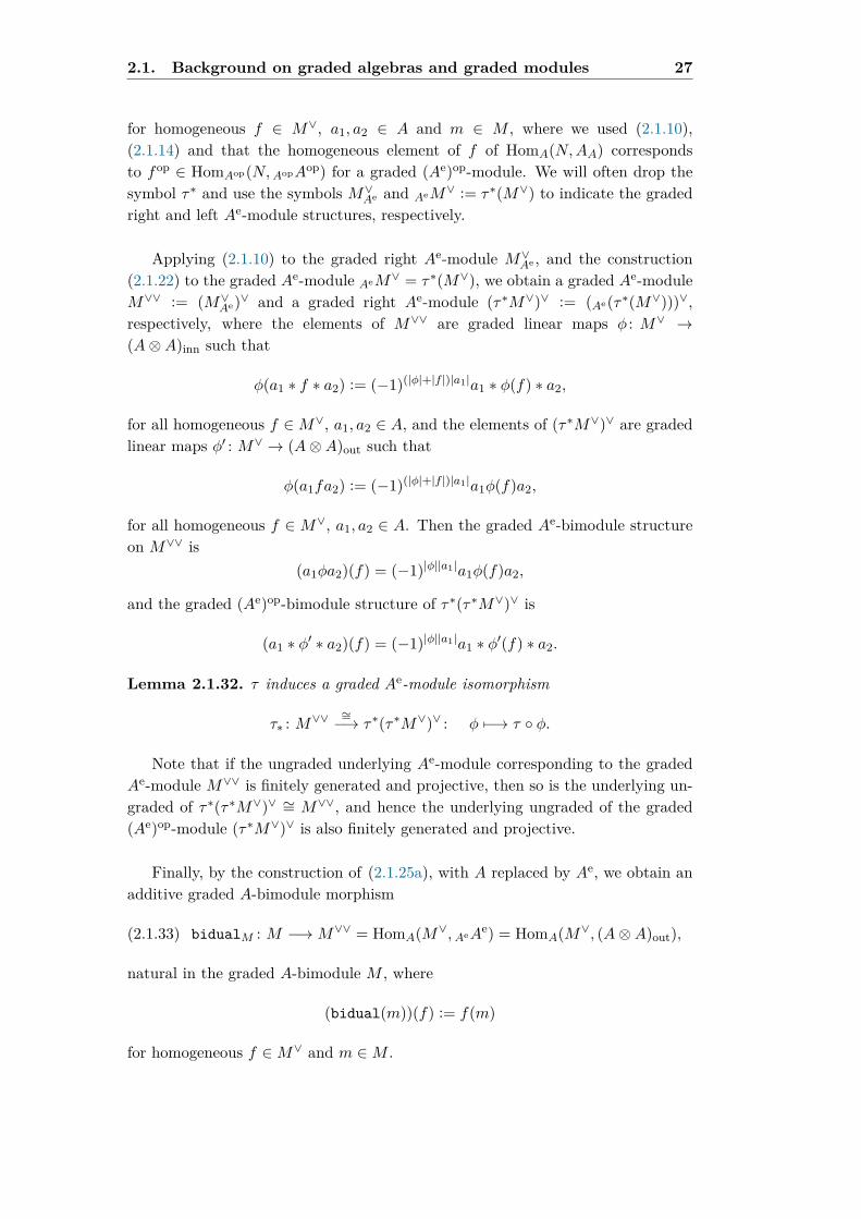
for homogeneous f ∈ M∨, a1, a2 ∈ A and m ∈ M , where we used (2.1.10),(2.1.14) and that the homogeneous element of f of HomA(N,AA) correspondsto fop ∈ HomAop(N,AopAop) for a graded (Ae)op-module. We will often drop thesymbol τ∗ and use the symbols M∨Ae and AeM∨ := τ∗(M∨) to indicate the gradedright and left Ae-module structures, respectively.
Applying (2.1.10) to the graded right Ae-module M∨Ae , and the construction(2.1.22) to the graded Ae-module AeM∨ = τ∗(M∨), we obtain a graded Ae-moduleM∨∨ := (M∨Ae)∨ and a graded right Ae-module (τ∗M∨)∨ := (Ae(τ∗(M∨)))∨,respectively, where the elements of M∨∨ are graded linear maps φ : M∨ →(A⊗A)inn such that
φ(a1 ∗ f ∗ a2) := (−1)(|φ|+|f |)|a1|a1 ∗ φ(f) ∗ a2,
for all homogeneous f ∈M∨, a1, a2 ∈ A, and the elements of (τ∗M∨)∨ are gradedlinear maps φ′ : M∨ → (A⊗A)out such that
φ(a1fa2) := (−1)(|φ|+|f |)|a1|a1φ(f)a2,
for all homogeneous f ∈ M∨, a1, a2 ∈ A. Then the graded Ae-bimodule structureon M∨∨ is
(a1φa2)(f) = (−1)|φ||a1|a1φ(f)a2,
and the graded (Ae)op-bimodule structure of τ∗(τ∗M∨)∨ is
(a1 ∗ φ′ ∗ a2)(f) = (−1)|φ||a1|a1 ∗ φ′(f) ∗ a2.
Lemma 2.1.32. τ induces a graded Ae-module isomorphism
τ∗ : M∨∨∼=−→ τ∗(τ∗M∨)∨ : φ 7−→ τ φ.
Note that if the ungraded underlying Ae-module corresponding to the gradedAe-module M∨∨ is finitely generated and projective, then so is the underlying un-graded of τ∗(τ∗M∨)∨ ∼= M∨∨, and hence the underlying ungraded of the graded(Ae)op-module (τ∗M∨)∨ is also finitely generated and projective.
Finally, by the construction of (2.1.25a), with A replaced by Ae, we obtain anadditive graded A-bimodule morphism
(2.1.33) bidualM : M −→M∨∨ = HomA(M∨,AeAe) = HomA(M∨, (A⊗A)out),
natural in the graded A-bimodule M , where
(bidual(m))(f) := f(m)
for homogeneous f ∈M∨ and m ∈M .

28 Basics on (graded) non-commutative algebraic geometry
2.1.2 Finitely generated projective modules
We will now collect the following results about finitely generated projective modulesover an associative algebra A.
(i) If M is a finitely generated and projective A-module, then M∨ is a finitelygenerated projective right A-module and the map
dualM : M −→M∨∨
of (2.1.25a) is an isomorphism of A-modules.
(ii) If M is a finitely generated projective A-module, then the map
evalM,N : M∨ ⊗A N −→ HomA(M,N)
of (2.1.25b) is an isomorphism, for any A-module N .
(iii) For modules AM , NA, BM ′ and BN′ over algebras A and B, the map ψ of
(2.1.27b) is an isomorphism, if M is a finitely generated projective A-moduleand M ′ is a finitely generated projective B-module.
(iv) For modules AM and AN and a vector space V (over k), the map
ψl : HomA(M,N)⊗ V −→ HomA(M,N ⊗ V )
in (2.1.28) is an isomorphism, provided that M is a finitely generatedprojective A-module. Similarly, if M is a finitely generated projective A-module, then the map
ψr : V ⊗HomA(M,N) −→ HomA(M,V ⊗N)
of (2.1.29) is an isomorphism.
For part (iv), note that it is a special case of part (iii), corresponding to two A-modulesM andN , for an algebra A, and a vector space V , because, in this case, themap ψl of (2.1.27b) becomes the map ψ : HomA(M,N)⊗ V → HomA(M,N ⊗ V )of (2.1.28).
Replacing now A by Ae, we obtain similar results for Ae-modules and (Ae)op-modules. In particular,
(v) If M is a finitely generated projective Ae-module, then M∨ is a finitelygenerated projective right Ae-module and the map bidualM : M → M∨∨
of (2.1.33) is an isomorphism of Ae-modules.
The proofs of these results are well-known and they can be found in a lot ofreferences (see, for instance, [64] or [66]). Finally, these formulae will be usedthroughout in this thesis for the underlying ungraded modules of graded modulesover graded algebras.

2.2. Basics on Noncommutative Algebraic Geometry 29
2.2 Basics on Noncommutative Algebraic Geometry
2.2.1 (Graded) Non-commutative differential 1-forms
In the rest of this chapter, we fix the following framework: let R be an associativek-algebra over a field of characteristic zero k, and A be a graded R-algebra, i.e. agraded algebra together with a graded algebra homomorphism R → A. Given agraded A-bimodule M , a derivation of weight n of A into M is an additive mapθ : A→M satisfying the Leibniz rule (see (2.3.10)):
(2.2.1) θ(ab) = (−1)n|a|θ(a)b+ aθ(b),
for all homogeneous a, b ∈ A, and an R-linear derivation of weight n of A into Mis a derivation of weight n, θ : A → M , which is a morphism θ : RAR → RMR ofgraded R-bimodules (equivalently, θ(R) = 0).
Based on the arguments introduced in §2.1, the space DernR(A,M) of R-linearderivations of weight n of A into M is a Z(Ae)-module. Furthermore,
DerR(A,M) :=⊕n∈Z
DernR(A,M)
is a graded Z(Ae)-module shall be called the space of graded derivations of A intoM . Note that, in particular, it is a graded k-module, because the image of k underthe structure map k → Ae is in Z(Ae).
Following [31], Section 2, and [75] for the graded setting, we define the gradedbimodule of non-commutative differential 1-forms as the graded A-bimodule Ω1
RA
endowed with an R-derivation of weight zero,
(2.2.2) d: A −→ Ω1RA : a 7−→ da,
which satisfies the following universal property: for every graded A-bimodule Mand R-linear derivation θ : A→M of weight |θ|, there exists a unique morphism ofgraded A-bimodules iθ : Ω1
RA→M such that θ = iθ d. In other words, the gradedA-bimodule Ω1
RA represents the functor DerR(A,−) from the category of gradedA-bimodules into the category of graded k-modules1 It is worthwhile to observethat |iθ| = |θ|.
Hence, by the universal property, there exists a canonical isomorphism of gradedA-bimodules,
(2.2.3) DerR(A,M)∼=−→ HomAe(Ω1
RA,M) : θ 7−→ iθ,
1 Explicitly, the bimodule Ω1RA is generated over A by the set of symbols da | a ∈ A under
the relations
(i) d(λ1a1 + λ2a2) = λ1 da1 + λ2 da2;(ii) d(a1a2) = a1(da2) + (−1)|a|(da1)a2,
for all λ1, λ2 ∈ k.

30 Basics on (graded) non-commutative algebraic geometry
whose inverse map is given by iθ 7→ θ = iθd . In particular, since iθ is a graded Ae-module morphism, iθ(a da) = (−1)|θ||a|a iθ(da) = (−1)|θ||a|aθ(a), for homogeneousa ∈ Ae, a ∈ A.
2.2.2 Graded Double Derivations and Non-commutative differen-tial forms
Let
(2.2.4) DerRA := DerR(A,AeAe) = DerR(A, (A⊗A)out)
be the graded Ae-module of double derivations, whose graded A-bimodule structurealso comes via the map (2.1.5) from Ae
Ae , or in other words, from the inner gradedA-bimodule structure (2.1.21b), i.e.,
(b ∗Θ ∗ c)(a) = (−1)|b||Θ′(a)|+|b||c|+|c||Θ′′(a)|Θ′(a)c⊗ bΘ′′(a),
for all homogeneous Θ ∈ DerRA, b ⊗ cop ∈ Ae and a ∈ A. Applying the functorHomAe(−AeAe) to Ω1
RA, we obtain a right graded Ae-module
(2.2.5) (Ω1RA)∨ = HomAe(Ω1
RA,AeAe) = HomAe(Ω1RA, (A⊗A)out),
which can be regarded as a graded A-bimodule and, as in §2.1.1, the graded A-bimodule structure comes via the map (2.1.5) (see (2.1.10)) from Ae
Ae , or in otherwords, from the inner graded A-bimodule structure (2.1.21b).
By the universal property (2.2.3) of Ω1RA, (2.2.4) and (2.2.5), we have the
canonical isomorphism:
(2.2.6)canonical : DerRA
∼=−→ (Ω1RA)∨
Θ 7−→ iΘ,
whereiΘ : Ω1
RA −→ A⊗A : α 7−→ (−1)|i′Θ(α)||i′′Θ(α)|σ(12)iΘα.
Observe that (2.2.6) is a graded Ae-module morphism because we are using thepermutation σ(12) : A ⊗ A → A ⊗ A : a1 ⊗ a2 7→ a2 ⊗ a1. The algebra ofnoncommutative differential forms of A is the tensor algebra
(2.2.7) Ω•RA := T•A Ω1RA
of the (graded) A-bimodule Ω1RA if n ≥ 0 whereas Ωn
RA = 0 if n < 0. Finally, byconvention, Ω0
RA = A.
Since A is a graded R-algebra, TA Ω1RA is a bi-complex. The grading by ‘form
degree’ will be denoted by || − || (and called the degree), whereas the gradinginduced from the A-grading shall be denoted by |−| (and called the weight). Itis important to observe that they interact by means of the so-called Koszul sign

2.2. Basics on Noncommutative Algebraic Geometry 31
convention, whereby the sign associated to two homogeneous elements a, b ∈ A ofbi-degrees ( || a || , |a|) and ( || b || , |b|) is (−1)( || a || ,|a|)·( || b || ,|b|), where
(2.2.8) ( || a || |a|) · ( || b || , |b|) := || a || · || b || +|a| · |b|.
Since Ω•R is a differential bi-graded algebra over A, we shall extend thedifferential d in (2.2.2) to a derivation in Ω•R of weight 0 and degree +1 using theLeibniz rule. Moreover, as Ω•RA is the free algebra of the graded bimodule Ω1
RA,there exists a unique extension of the map iΘ : Ω1
RA→ A⊗A to a double derivationof bi-degree (−1, |Θ|) on TA Ω1
RA with respect to the bigrading ( || − || , |−|),
(2.2.9) iΘ : Ω•RA −→⊕
(ΩiRA⊗ Ωj
RA),
where the sum is over pairs (i, j) with i+ j = • − 1.
As we wrote above, in particular, iΘ is a double derivation for a homogeneousΘ ∈ DerRA and satisfies the following Leibniz rule:
(2.2.10)iΘ(αβ) = (−1)|Θ||α|(iΘα)β + (−1) || α || || iΘ || α(iΘβ)
= (−1)|Θ||α|(iΘα)β + (−1)|| α ||α(iΘβ).
Observe that the map iΘ should be regarded as a super-derivation of the gradedalgebra Ω•RA with coefficients in Ω•RA ⊗ Ω•RA, viewed as an Ω•RA-bimodule withrespect to the outer bimodule structure. In particular, if da,db ∈ Ω1
RA, by (2.2.10),
(2.2.11)iΘ(da db) = (−1)|Θ||a|iΘ(da) db− daiΘ(db)
= (−1)|Θ||a|(Θ′(a)⊗Θ′′(a))(1⊗ db)− (da⊗ 1)(Θ′(b)⊗Θ′′(b)
= (−1)|Θ||a|Θ′(a)⊗ (Θ′′(a) db)− (daΘ′(b))⊗Θ′′(b).
Finally, we point out that for every homogeneous element a ∈ A, we have iΘ(a) = 0if Θ ∈ DerRA because |iΘ| = −1. The Lie derivative with respect to Θ ∈ DerRAis the map
LΘ : Ω1RA −→ (A⊗ Ω1
RA)⊕ (Ω1RA⊗A)
defined on generators by LΘ(a) = Θ(a) and LΘ(da) = dΘ(a), for homogeneousa ∈ A, and we extend it to Ω1
RA by imposing the Leibniz rule. By a simplecalculation on the generators, one obtains the Cartan formula in this setting(see [30, (2.7.2)]):
Lemma 2.2.12.LΘ = d iΘ + iΘ d.
Moreover, the Lie derivative LΘ extends to a degree 0 derivation and weight|Θ|,
(2.2.13) LΘ : Ω•RA→⊕(
ΩiRA⊗ Ωj
RA)⊂ (Ω•RA)⊗2,

32 Basics on (graded) non-commutative algebraic geometry
where the sum is now for pairs (i, j) with i+ j = •. A key technical point in non-commutative algebraic geometry is the fact that for every associative k-algebra A,the bi-complex (Ω•kA, d ) has trivial cohomology:
H i(Ω•kA,d) =k if i = 0,0 if i > 0.
As it is explained in [41], §11.4, we have an isomorphism ΩpkA = A⊗ (A/k)⊗p, and
the differential d corresponds to the natural projection
A⊗ (A/k)⊗p −→ (A/k)⊗ (A/k)⊗p ' k ⊗ (A/k)⊗(p+1) ⊂ A⊗ (A/k)⊗(p+1)
The kernel of the latter projection is equal to k⊗(A/k)⊗p, which is exactly the imageof the differential d: A ⊗ (A/k)⊗(p−1) −→ k ⊗ (A/k)⊗p. To obtain an interestingcohomology, we consider the commutator quotient of the complex (Ω•RA,d ). LetA be a graded R-algebra and define the non-commutative Karoubi-de Rham bi-complex of A as the bi-graded vector space
DR•R (A) := Ω•RA/[Ω•RA,Ω•RA],
where if ω, ω′ ∈ Ω•RA, their bi-graded commutator is defined as (see [98])
[ω, ω′] := ωω′ − (−1)( || ω || || ω′ || +|ω||ω′|)ω′ω,
where we denote the bi-gradation of DR•R (A) as in Ω•RA and we use the Koszulconvention (2.2.8). Finally, the differential d : Ω•RA → Ω•+1
R A descends to a well-defined differential d : DR•R (A) → DR•+1
R (A) and hence the Karoubi-de Rhambi-complex becomes a differential bi-graded vector space.
Given a graded R-algebra C and c = c1 ⊗ c2, with ci ∈ C, define
c := (−1)|c1||c2|c2 ⊗ c1,
and given a linear map φ : C −→ C⊗2, write
φ : C −→ C : c 7−→ (φ(c)).
In our case, C = Ω•RA which is bi-graded, hence we have to deal with the weightinherited from A and the degree as differential form. Thus, if Θ ∈ DerRA,
(2.2.14)iΘ : Ω•RA −→ Ω•RA⊗ Ω•RA
α 7−→ iΘ(α) := (−1) || i′Θ(α) || || i′′Θ(α) || +|i′Θ(α)||i′′Θ(α)|i′′Θ(α)⊗ i′Θ(α)
Moreover, define an operation between non-commutative differential forms:
(2.2.15)m : Ω•RA⊗ Ω•RA −→ Ω•RA
α⊗ β 7−→ m(α⊗ β) := αβ

2.2. Basics on Noncommutative Algebraic Geometry 33
Combining (2.2.14) and (2.2.15), we are able to define the desired operator; thereduced contraction operator for a homogeneous Θ ∈ DerRA and a bi-homogeneousα ∈ Ω•RA defined as
(2.2.16)ιΘ : Ω•RA −→ Ω•RA
α 7−→ ιΘα,
where
(2.2.17) ιΘα := (−1) || i′Θ(α) || || i′′Θ(α) || +|i′Θ(α)||i′′Θ(α)|i′′Θ(α)i′Θ(α).
Similarly, we define the reduced Lie derivative
(2.2.18) LΘ := LΘ : Ω•RA −→ Ω•RA.
We apply the operation (−) to the Cartan formula in Lemma 2.2.12, obtainingthe reduced Cartan identity which relates LΘ and ιΘ:
Lemma 2.2.19 ([30], Lemma 2.8.8). For every homogenous Θ ∈ DerRA,
LΘ = d ιΘ + ιΘ d.
2.2.3 Smoothness
In this subsection we shall introduce the concept of smoothness which will be usedthroughout in this thesis. Recall (see [72]) that an associative algebra A is calledformally smooth if the following lifting property holds: for every algebra B and anilpotent two-sided ideal I ⊂ B (that is, I = BIB and In = 0 for n 0), given amap A→ B/I, there is a lift A→ B such that the following diagram commutes
(2.2.20) B
A //
==
B/I
where B → B/I is the quotient map. The definition of formal smoothness viathe lifting property (2.2.20) is analogous to Grothendieck’s definition of formallysmooth algebras in the commutative case.
From now on, let R be an associative k-algebra over a field of characteristiczero and A is an R-algebra. Then to obtain a notion of nonsingularity for non-commutative algebras, W. F. Schelter proved in [84] (see also [31], Proposition 3.2)the following result:
Proposition 2.2.21 ([84], Lemma 2.3). An R-algebra A is formally smooth if andonly if the A-bimodule Ω1
RA is projective.
Motivated by this result, following [31] and [31], we make the following

34 Basics on (graded) non-commutative algebraic geometry
Definition 2.2.22. An R-algebra A is called smooth over R if it is finitelygenerated as an R-algebra and Ω1
RA is projective as an Ae-module.
Proposition 2.2.23. If A is smooth over R and M is a finitely generated andprojective A-bimodule, the algebra A = TAM is also smooth over R.
Proof. [31], Proposition 5.3(3).
2.2.4 The (iso)morphism bidualΩ1RA
Let A be a graded smooth R-algebra. Applying (v) in §2.1.2 to M = Ω1RA, we
obtain the following isomorphism of graded A-bimodules:
(2.2.24)bidualΩ1
RA: Ω1
RA∼=−→ (Ω1
RA)∨∨
α 7−→ α∨,
where
(Ω1RA)∨∨ = HomA((Ω1
RA)∨, AeAe) = HomA((Ω1
RA)∨, (A⊗A)inn),
and α∨(f) = f(α) for homogeneous f ∈ (Ω1RA)∨. Dualizing now the isomorphism
(2.2.6), we obtain
(2.2.25) (canonical)∨ : (Ω1RA)∨∨
∼=−→ (DerRA)∨ : ϕ 7→ i∨(ϕ),
where
i∨(ϕ) : DerRA −→ A⊗AΘ 7−→ i∨(ϕ)(Θ) = ϕ(iΘ).
Composing the isomorphisms (2.2.24) and (2.2.25), we obtain the followingisomorphism
(2.2.26)Bidual′ : Ω1
RA∼=−→ (DerRA)∨
α 7−→ i∨(α∨),
where
i∨(α∨) : DerRA −→ A⊗A : Θ 7−→ (−1)|i′Θ(α)||i′′Θ(α)|σ(12)iΘα
By part (iv) of §2.1.2 applied to the graded algebra Ae, given a graded A-bimodule M and a graded vector space V , we obtain an isomorphism
(2.2.27) ψl : HomAe(Ω1RA,M)⊗ V
∼=−→ HomAe(Ω1RA,M ⊗ V ),
where the graded A-bimodule structure on the ‘external’ tensor product M ⊗ Vcomes from the graded A-bimodule M , i.e. the multiplication is given by(a1 ⊗ aop
2 )(m ⊗ v) = ((a1 ⊗ aop2 )m) ⊗ v for homogeneous a1 ⊗ aop
2 ∈ Ae, m ∈ M ,

2.3. Graded double Poisson structures 35
v ∈ V . This is used in [96] when M = AeAe = (A⊗A)out and V = A. In this case,we have an isomorphism of graded A-bimodules given by
(2.2.28)τ(23) : AeAe ⊗A
∼=−→ A⊗3
(a1 ⊗ a2)⊗ a3 7−→ (−1)|a2||a3|a1 ⊗ a3 ⊗ a2,
where in the right-hand side, A⊗3 has its outer graded A-bimodule structure. Thisisomorphism induces another one, that will also be denoted τ(23):
(2.2.29) τ(23) : HomAe(Ω1RA,AeAe⊗A)
∼=−→ HomAe(Ω1RA,A
⊗3)∼=−→ DerR(A,A⊗3)
Using (2.2.27) for M = AeAe and V = A, (2.2.28) and (2.2.29),
(2.2.30)
DerRA⊗A = HomAe(Ω1RA,AeAe)⊗A
∼= HomAe(Ω1RA,AeAe ⊗A)
∼= HomAe(Ω1RA,A
⊗3)∼= DerR(A,A⊗3).
Similarly, under the same assumptions on A, M and V , and by part (iv) in§2.1.2, we obtain an isomorphism
(2.2.31) ψr : V ⊗HomAe(Ω1RA,M)
∼=−→ HomAe(Ω1RA, V ⊗M).
Taking M = AeAe = (A⊗A)out and V = A, we have the following isomorphism ofgraded A-bimodules:
(2.2.32)τ(12) : A⊗ AeAe ∼=−→ A⊗3
a1 ⊗ (a2 ⊗ a3) 7−→ (−1)|a1||a2|a2 ⊗ a1 ⊗ a3,
where in the right-hand side, A⊗3 has its outer graded A-bimodule structure. Thisisomorphism induces another one, that will also be denoted τ(12):
(2.2.33) τ(12) : HomAe(Ω1RA,AeAe)
∼=−→ HomAe(Ω1RA,A
⊗3)∼=−→ DerR(A,A⊗3).
Now, applying the isomorphisms (2.2.31) for M = AeAe and V = A, (2.2.32) and(2.2.33):
(2.2.34)
A⊗ DerRA = A⊗HomAe(Ω1RA,AeAe)
∼= HomAe(Ω1RA,A⊗ AeAe)
∼= HomAe(Ω1RA,A
⊗3)∼= DerR(A,A⊗3)
2.3 Graded double Poisson structures
2.3.1 Double Poisson algebras of weight −N
Commutative Poisson algebras appear in several geometric and algebraic contexts.As a direct non-commutative generalization, one might consider associative al-gebras that are at the same time Lie algebras under a ‘Poisson bracket’ −,−

36 Basics on (graded) non-commutative algebraic geometry
satisfying the Leibniz rules ab, c = ab, c + a, cb, a, bc = ba, c + a, bc.However such Poisson brackets are the commutator brackets up to a scalar multi-ple, provided the algebra is prime and not commutative [36, Theorem 1.2]. A wayto resolve this apparent lack of noncommutative Poisson algebras is provided bydouble Poisson structures, introduced by M. Van den Bergh in [96], §2.2.
An n-bracket on an associative algebra A is a linear map
−, · · · ,− : A⊗n −→ A⊗n,
which is a derivation A→ A⊗n in its last argument for the outer bimodule structureon A⊗n, i.e.
a1, a2, ..., an−1a′n
= an−1
a1, a2, ..., a
′n
+ a1, a2, ..., an−1 a′n
and which is cyclically anti-symmetric in the sense
τ(1···n) −, · · · ,− τ−1(1···n) = (−1)n+1 −, · · · ,− .
If A is an R-algebra, then an n-bracket is R-linear if it vanishes when its lastargument is in the image of R. Observe that a 1-bracket is a derivation. Next, let−,− be a double bracket on A, a ∈ A, and b = b1 ⊗ · · · ⊗ bn ∈ A⊗n. Then wedefine
a, bL = a, b1 ⊗ b2 ⊗ · · · ⊗ bn,a, bR = b1 ⊗ · · · ⊗ bn−1 ⊗ a, bn ,
which enables us to introduce an appropriate analogue of the Jacobi identity inthis setting:
Definition 2.3.1 (Double Poisson algebra [96]). A double bracket on A is a linearmap
−,− : A⊗A −→ A⊗A,
which satisfies, for all a, b, c ∈ A,
a, b = −σ(12) b, a ,(2.3.2a)a, bc = b a, c+ a, b c.(2.3.2b)
Furthermore, a double bracket −,− on A is a double Poisson bracket if satisfiesthe double Jacobi identity:
(2.3.3) 0 = a, b, cL + σ(123) b, c, aL + σ(132) c, a, bL .
An algebra with a double Poisson bracket (A, −,−) is a double Poisson algebra.
Remark 2.3.4. Observe that (2.3.2a) can be rewritten as
a, b = −b, a ,
where we used the operator (−) introduced in §2.2.2.

2.3. Graded double Poisson structures 37
Moreover, note that the formulas (2.3.2a) and (2.3.2b) imply that −,− isa derivation A → A ⊗ A in its first argument for the inner bimodule structure onA⊗A, that is,
ab, c = a ∗ b, c+ a, c ∗ b,
where, as usual, by ∗ we mean the inner action and a, b ∈ A.
If −,− is a double bracket, M. Van den Bergh defined in [96], §2.4, thebracket associated to −,−:
(2.3.5) −,− : A⊗A −→ A : (a, b) 7−→ a, b := m a, b = a, b′ a, b′′
Here m denotes the multiplication. It is clear that −,− is a derivation in itssecond argument. Recall (see [?]) that a left Loday algebra is a vector space Vequipped with a bilinear operation [−,−] such that the following version of theJacobi identity is satisfied:
[a, [b, c]] = [[a, b], c] + [b, [a, c]],
for all a, b, c ∈ V .
Proposition 2.3.6. Let A be a double Poisson algebra. Then
(2.3.7) a, b, c − a, b, c − b, a, c = 0,
(2.3.8) a, b, c = a, b, c+ b, a, c,
where, in (2.3.7), a,− acts on tensors by a, u ⊗ v = a, u ⊗ v + u ⊗ a, v,for all a, u, v ∈ A. In fact, (A, −,−) is a left Loday algebra.
Proof. All the statements are immediate consequences of [96], Proposition 2.4.2(in fact, (2.3.8) is [96], Corollary 2.4.4).
In [96], §2.7, M. Van den Bergh introduced the notion of double Gerstenhaberalgebra (see, for instance, [96] Theorem 3.2.2). In the last part of this subsection,we shall define double Poisson algebras of weight −N (the graded extension ofdouble Poisson algebras) in such a way that Van den Bergh’s double Gerstenhaberalgebras will be double Poisson algebras of weight -1.
Let Vi, i = 1, ..., n be graded vector spaces, a = a1 ⊗ · · · ⊗ an a homogeneouselement of V1 ⊗ · · · ⊗ Vn and s ∈ Sn be a permutation, then
σs(a) = (−1)tas−1(1) ⊗ · · · ⊗ as−1(n),
wheret =
∑i<j
s−1(i)>s−1(j)
|as−1(i)||as−1(j)|.

38 Basics on (graded) non-commutative algebraic geometry
Definition 2.3.9 (Double Poisson algebra of weight −N). Let R be an associativek-algebra over a field of characteristic zero. Let A be a graded R-algebra andN ∈ Z≥0. A double bracket of weight −N on A is a graded R-bilinear map
−,− : A⊗A −→ A⊗A
of weight −N such that the following identities hold:
a, bc = (−1)(|a|−N)|b|b a, c+ a, b c,(2.3.10)
a, b = −σ(12)(−1)(|a|−N)(|b|−N) b, a .(2.3.11)
Furthermore, a double bracket of weight −N , −,− on A, is a double Poissonbracket of weight −N if satisfies the graded double Jacobi identity:
(2.3.12)0 = a, b, cL + (−1)(|a|−N)(|b|+|c|)σ(123) b, c, aL +
+ (−1)(|c|−N)(|a|+|b|)σ(132) c, a, bL .
An algebra with a double Poisson bracket of weight −N (A, −,−) is a doublePoisson algebra of weight −N (over R).
2.3.2 Poly-vector fields and the graded double Schouten–Nijenhuis bracket
A very useful description of Poisson brackets on a commutative smooth variety Xis in terms of bivector fields, i.e., sections P of
∧2 TX , such that P, P = 0, wherethe Schouten–Nijenhuis bracket −,− determines a structure of Gerstenhaberalgebra on the graded algebra
∧• TX of poly-vector fields. Let R be an associativealgebra and A be a graded smooth R-algebra, then we will now describe the non-commutative counterpart to the Schouten–Nijenhuis bracket on TADerRA.
Proposition 2.3.13. Let homogeneous Θ,∆ ∈ DerRA. Then
Θ,∆∼l = (Θ⊗ 1)∆− (1⊗∆)Θ,Θ,∆∼r = (1⊗Θ)∆− (∆⊗ 1)Θ = −∆,Θ∼l ,
define graded derivations A → A⊗3, where the bimodule structure on A⊗3 is thegraded outer structure.
Proof. It is an adaptation to the graded setting of [96], Proposition 3.2.1.
Since A is a graded smooth R-algebra, by (iv) in §2.1.2, (2.2.30) and (2.2.34),we can define
Θ,∆l := τ(23) Θ,∆∼l , Θ,∆r := τ(12) Θ,∆∼r
as elements of DerRA⊗A and A⊗DerRA, respectively, and where τ(23) and τ(12)are given by (2.2.28) and (2.2.32), respectively.

2.3. Graded double Poisson structures 39
Finally, given homogeneous a, b ∈ A and Θ,∆ ∈ DerRA, we define
(2.3.14)a, b = 0,Θ, a = Θ(a),Θ,∆ = Θ,∆l + Θ,∆r ,
with the right-hand sides in (2.3.14) viewed as elements of (TADerRA)⊗2.The graded double Schouten–Nijenhuis bracket is the unique extension−,− : (TADerRA)⊗2 → (TADerRA)⊗2 of (2.3.14) of weight -1 to the tensoralgebra TADerRA satisfying the graded Leibniz rule (see (2.3.10)):
(2.3.15) ∆,ΘΦ = (−1)(|∆|−1)|Θ|Θ ∆,Φ+ ∆,ΘΦ,
for homogeneous ∆,Θ,Φ ∈ TADerRA.
2.3.3 Differential double Poisson algebras
Let B be an associative algebra and A be a graded smooth B-algebra. Then M.Van den Bergh [96, Proposition 4.1.2] proved that there exists an isomorphismbetween (TADerB A)n and B-linear n-brackets on A:
(2.3.16) µ : Q 7−→ −, · · · ,−Q ,
which on Q = δ1 · · · δn (δi ∈ DerB A for all i) is given by
(2.3.17) −, · · · ,−Q =n−1∑i=0
(−1)(n−1)iτ i(1...n) −, · · · ,−∼Q τ
−i(1...n),
where
a1, ..., an∼Q = δn(an)′δ1(a1)′′ ⊗ δ1(a1)′δ2(a2)′′ ⊗ · · · ⊗ δn−1(an−1)′δn(an)′′).
It is important to note that the map µ in (2.3.16) factors throughTADerB A/[TADerB A,TADerB A]. In addition, M. Van den Bergh proved in [96],Proposition 4.1.2 that if A is smooth over B, then µ is an isomorphism. Never-theless, the calculation of −, · · · ,−Q using (2.3.17) may be difficult in practice.The following result overcomes this problem:
Proposition 2.3.18 ([96], Proposition 4.2.1). For Q ∈ (TADerB A)n (an n-foldof the tensor algebra), the following identity holds
(2.3.19) a1, ..., anQ = (−1)n(n−1)
2 a1, ..., an−1, Q, anL · · · L ,
for all all a1, ..., an ∈ A.
The subsequent result will be interesting because in the right hand side we shallobtain the double Jacobi identity for the bracket −,−P :

40 Basics on (graded) non-commutative algebraic geometry
Proposition 2.3.20 ([96], Proposition 4.2.2). Let P ∈ (TADerB A)2. We havethe following identity for a, b, c ∈ A:
−12 a, b, P, P, c =
= a, b, cP P,L + τ(123) b, c, aP P,L + σ(132) c, a, bP P,L .
Hence this result enables us to introduce a new concept:
Definition 2.3.21 (DDP). We say that A is a differential double Poisson algebra(a DDP for short) over B if it is equipped with an element P ∈ (TADerB A)2 (adifferential double Poisson bracket) such that
(2.3.22) P, P = 0 mod [TADerB A,TADerB A].
By Proposition 2.3.20, it is clear that if (A,P ) is a differential double Poissonalgebra then A is a double Poisson algebra with double bracket −,−P . In thesmooth case, since µ in (2.3.16) is an isomorphism, the notions of differential doublePoisson algebra and double Poisson algebra coincide.
2.4 Bi-symplectic structures
Following [30] and [96], Appendix A, in this section we introduce the crucial notionof bi-symplectic algebras which we will extend to other settings below:
Definition 2.4.1. Let A be an associative k-algebra over a field of characteristiczero. An element ω ∈ DR2(A) is bi-non-degenerate if the map of A-bimodules (see(2.2.16))
ι(ω) : DerA −→ Ω1A : Θ 7−→ ιΘω
is an isomorphism. If in addition ω is closed in DR•(A), then we say that ω isbi-symplectic. An associative k-algebra A endowed with a bi-symplectic form ω
(A,ω) will be called a bi-symplectic algebra.
Let ω ∈ DR2(A) be a bi-symplectic form. We define the Hamiltonian doublederivation Ha ∈ DerA corresponding to a ∈ A via
(2.4.2) ιHaω = da,
and write
(2.4.3) a, bω = Ha(b) ∈ A⊗A
Since Ha(b) = iHa(db), (2.4.3) can be written in the following form:
(2.4.4) a, bω = iHaιHbω,
which is more convenient to prove that −,−ω is a double bracket on A (see[96], Lemma A.3.2). Furthermore, the following result shows that double Poissonbrackets on associative algebras and bi-symplectic algebras are closely related:

2.5. Definition of bi-symplectic associative N-algebras 41
Lemma 2.4.5 ([96], Proposition A.3.3). If (A,ω) is a bi-symplectic algebra, then−,−ω is a double Poisson bracket on A.
Finally, the following result describes how the Hamiltonian double derivationinterchanges double Poisson brackets and double Schouten–Nijenhuis brackets:
Proposition 2.4.6 ([96, Proposition 3.5.1]). The following are equivalent:
(i) −,− is a double Poisson bracket on A.
(ii) Ha, Hbl = Ha,b′ ⊗ a, b′′, for all a, b ∈ A.
(iii) Ha, Hbr = a, b′ ⊗H ′′a,b, for all a, b ∈ A.
(iv) Ha, Hb = Ha,b, for all a, b ∈ A, where Hx := Hx′ ⊗ x′′ + x′ ⊗ Hx′′ forall x = x′ ⊗ x′′ ∈ A⊗A.
2.5 Definition of bi-symplectic associative N-algebras
In this subsection, let R be an associative k-algebra, with k a field of characteristiczero. Following [30], §2.7, the weights in A give rise to the Euler derivation
Eu: A −→ A,
defined by Eu|Aj = j · Id for j = 0, 1, .... The action of the corresponding Liederivative operator
(2.5.1) LEu : DR•R (A)→ DR•R (A)
has nonnegative integral eigenvalues. As usual all canonical objects (forms, doublederivations,...) acquire weights by means of this operator.
Definition 2.5.2. Let B be an associative R-algebra.
(i) An associative N-algebra over B (shorthand for ‘non-negatively gradedalgebra’) is a Z-graded associative B-algebra A such that Ai = 0 for alli < 0. We say a ∈ A is homogeneous of weight |a| = i if a ∈ Ai.
(ii) A tensor N-algebra over B is an associative N-algebra A over B which can bewritten as a tensor algebra A = TBM , for a positively graded B-bimoduleM , so M =
⊕i∈ZM
i, where M i = 0 for i ≤ 0.
(iii) We say m ∈M is homogeneous of weight |m| = i if m ∈M i.
(iv) The weight of an associative N-algebra A is |A| := minS∈G
maxa∈S|a|, where the
elements of G are the finite sets of homogeneous generators of A.
Bi-symplectic forms over associative N-algebras will be key ingredients in thisthesis.

42 Basics on (graded) non-commutative algebraic geometry
Definition 2.5.3. Let A be an associative N-algebra over B. An elementω ∈ DR2
R (A) which is closed for the universal derivation d is a bi-symplectic formof weight N if
(i) LEuω = Nω for the operator (2.5.1), and
(ii) the following map of graded A-bimodules is an isomorphism:
ι(ω) : DerRA −→ Ω1RA[−N ] : Θ 7−→ ιΘω.
An associative N-algebra equipped with a bi-symplectic form of weight N (A,ω) iscalled a bi-symplectic associative N-algebra of weight N (over B).
Following [98], [30] and §2.4, if ω ∈ DR2R (A) is a bi-symplectic form of weight
N , using the Hamiltonian double derivation Ha ∈ DerRA corresponding to anhomogenous a ∈ A (see (2.4.2)), we can write
(2.5.4) a, bω = iHaιHbω,
The crucial point for our construction is that −,−ω just introduced is a doublePoisson bracket of weight −N (see Definition 2.3.9 and Proposition 2.4.5):
Lemma 2.5.5. If (A,ω) is a bi-symplectic associative N-algebra of weight N overB, then −,−ω is a double Poisson bracket of weight −N on A.
Proof. It is a graded version of [96], Proposition A.3.3. To determine theweight of −,−ω, observe that by (2.4.2), |Ha| + |ω| = |a| and by (2.4.3),|a, bω| = |a|+ |b| − |ω|. Thus, −,−ω = −N .
Now, if ω is a bi-symplectic form of weight k on a graded R-algebra A, wesay that an homogeneous double derivation Θ ∈ DerRA is bi-ymplectic if thereduced Lie derivative (2.2.18) of ω along Θ vanishes. In other words, LΘω = 0.Moreover, as in the commutative case, bi-symplectic forms of weight k imposestrong constrains over associative N-algebras, as the following result shows:
Lemma 2.5.6. Let ω be a bi-symplectic form of weight j 6= 0 on a associativeN-algebra A over R. Then
(i) ω is exact.
(ii) If Θ is a bi-symplectic double derivation of weight l, if j + l 6= 0, then Θ is aHamiltonian double derivation.
Proof. (i) Since ω is a bi-symplectic form of weight j 6= 0, by definition,
LEuω = jω,
where LEu is the operator LEu : DR•R (A) → DR•R (A) introduced in (2.5.1). Now,by the Cartan identity,
jω = LEuω = diEuω,

2.6. The Kontsevich–Rosenberg principle for bi-symplectic forms 43
and (i) holds. To prove (ii), using that Θ is a bi-symplectic form and Lemma 2.2.19we obtain
(2.5.7) 0 = LΘω = dιΘω.
We take H := iEuιΘω, where iEu : DR•R (A)→ DR•R (A) is the contraction operatorbecause Eu ∈ DerRA, we get
dH = d(iEuιΘω) = LEu(ιΘω) = |ιΘω|ιΘω = (l + j)ιΘω,
where in the second identity we used (2.5.7).
2.6 The Kontsevich–Rosenberg principle for bi-symplectic forms
This subsection is devoted to show how the Kontsevich–Rosenberg principle worksfor some geometric structures relevant for this thesis. We follow [30], §6.2, closely.
Let R be a semisimple finite-dimensional k-algebra over a field of characteristiczero k, and V an R-module. Observe that the action of R gives an algebra mapR → Homk(V, V ), making End(V ) := Homk(V, V ) an R-algebra. If A is a finitelygenerated associative R-algebra, Rep(A, V ) is an affine scheme of finite type overk.
For sake of simplicity, we write AV := k[Rep(A, V )]. We consider AV ⊗End(V ),a tensor product of associative algebras, which also is an R-algebra via the mapR → End(V ). Let GL(V )R be the group of R-module automorphisms of V , andGm ⊂ GL(V )R is the one-dimensional torus of scalar automorphisms of V . Wedefine G := GL(V )R/Gm. Observe that the action of G on V makes Rep(A, V ) aG-scheme. This gives a G-action on AV by algebra automorphisms. We also have aG-action on End(V ), by conjugation, and G acts diagonally on AV ⊗End(V ). Wewrite AGV and (AV ⊗ End(V ))G for the corresponding subalgebra of G-invariants.
To each element a ∈ A, we can associate the evaluation functiona : Rep(A, V ) → End(V ) : ρ 7→ ρ(a). The assignment a 7→ a gives rise an asso-ciative R-algebra homomorphism
ev : A→ (AV ⊗ End(V ))G : a 7−→ a.
If we compose the function a with the trace map Tr: End(V ) → k applied tothe second tensor factor of (AV ⊗ End(V ))G above, we obtain a G-invariant el-ement Tr a ∈ AGV . If a ∈ [A,A], then Tr a = 0 because the symmetry of thetrace. Therefore, the assignment a → Tr a gives a well-defined k-linear mapTr ev : A/[A,A] → AGV . So, due to the Kontsevich–Rosenberg principle, we canregard A/[A,A] as the space of non-commutative functions.

44 Basics on (graded) non-commutative algebraic geometry
To study this principle for differential forms, we use a natural evaluation map ondifferential forms which sends the Karoubi de-Rahm complex of A to the ordinaryde Rham complex of the representation scheme. We write
Ω•(Rep(A, V )) =∧•
AVΩ1(Rep(A, V ))
for the (ordinary) differential graded algebra of algebraic differential forms on thescheme Rep(A, V ). We have an algebra homomorphism
ev : ΩnA→ (Ωn(Rep(A, V ))⊗ End(V ))G : α = a0 da1...dan 7→ α = a0da1...d an,
defined as the following composite (observe that ΩnA = A⊗ (A/k)⊗n, see [31])
A⊗ (A/k)⊗n ev−→ (AV ⊗ End(V ))⊗ Ω1(Rep(A, V ))⊗ End(V )⊗n
−→ (∧n
AVΩ1(Rep(A, V )))⊗ (End(V ))⊗n+1
Id⊗m−→ Ωn(Rep(A, V ))⊗ End(V ).
As r is a constant function, for any r ∈ R, we have dr = 0. It follows that the mapabove induces a well defined differential graded algebra morphism
Ω•RA −→ (Ω•(Rep(A, V ))⊗ End(V ))G .
Furthermore, composing the latter morphism with the trace map Id ⊗Tr: Ω•(Rep(A, V ))⊗ End(V )→ Ω•(Rep(A, V )), we obtain a linear map
Tr ev : DR•R (A) −→ Ω•(Rep(A, V ))G : α 7−→ Tr α.
Note that the previous map commutes with the de Rham differentials.
Next, we will apply the Kontsevich–Rosenberg principle to bi-symplectic forms.We will prove that Tr ω is a symplectic form following closely [30], Theorem6.4.3(ii).
We fix ρ ∈ Rep(A, V ) and we see V = Vρ as an A-module and EndVρas an A-bimodule. Also, we denote (EndVρ)∗ := Hom(Vρ, k). Finally, ob-serve that the trace pairing (u, v) 7→ Tr(uv) gives an A-bimodule isomorphismtr : (EndVρ)∗
∼=−→ EndVρ.
Now, the Zariski tangent space to the affine scheme Rep(A, V ) (see [22]) at thepoint ρ ∈ Rep(A, V ) is
Tρ Rep(A, V ) = DerR(A,EndVρ) = HomAe(Ω1RA,EndVρ).
Therefore, we can write the cotangent space at the same point ρ ∈ Rep(A, V ):
T∗ρ Rep(A, V ) = (DerR(A,EndVρ))∗ = (HomAe(Ω1RA,EndVρ))∗.
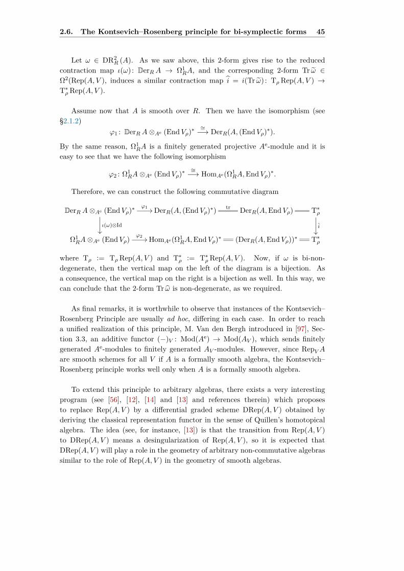
2.6. The Kontsevich–Rosenberg principle for bi-symplectic forms 45
Let ω ∈ DR2R (A). As we saw above, this 2-form gives rise to the reduced
contraction map ι(ω) : DerRA → Ω1RA, and the corresponding 2-form Tr ω ∈
Ω2(Rep(A, V ), induces a similar contraction map i = i(Tr ω) : Tρ Rep(A, V ) →T∗ρ Rep(A, V ).
Assume now that A is smooth over R. Then we have the isomorphism (see§2.1.2)
ϕ1 : DerRA⊗Ae (EndVρ)∗∼=−→ DerR(A, (EndVρ)∗).
By the same reason, Ω1RA is a finitely generated projective Ae-module and it is
easy to see that we have the following isomorphism
ϕ2 : Ω1RA⊗Ae (EndVρ)∗
∼=−→ HomAe(Ω1RA,EndVρ)∗.
Therefore, we can construct the following commutative diagram
DerRA⊗Ae (EndVρ)∗ϕ1 //
ι(ω)⊗Id
DerR(A, (EndVρ)∗) tr DerR(A,EndVρ) T∗ρ
i
Ω1RA⊗Ae (EndVρ)
ϕ2 // HomAe(Ω1RA,EndVρ)∗ (DerR(A,EndVρ))∗ T∗ρ
where Tρ := Tρ Rep(A, V ) and T∗ρ := T∗ρ Rep(A, V ). Now, if ω is bi-non-degenerate, then the vertical map on the left of the diagram is a bijection. Asa consequence, the vertical map on the right is a bijection as well. In this way, wecan conclude that the 2-form Tr ω is non-degenerate, as we required.
As final remarks, it is worthwhile to observe that instances of the Kontsevich–Rosenberg Principle are usually ad hoc, differing in each case. In order to reacha unified realization of this principle, M. Van den Bergh introduced in [97], Sec-tion 3.3, an additive functor (−)V : Mod(Ae) → Mod(AV ), which sends finitelygenerated Ae-modules to finitely generated AV -modules. However, since RepVAare smooth schemes for all V if A is a formally smooth algebra, the Kontsevich–Rosenberg principle works well only when A is a formally smooth algebra.
To extend this principle to arbitrary algebras, there exists a very interestingprogram (see [56], [12], [14] and [13] and references therein) which proposesto replace Rep(A, V ) by a differential graded scheme DRep(A, V ) obtained byderiving the classical representation functor in the sense of Quillen’s homotopicalalgebra. The idea (see, for instance, [13]) is that the transition from Rep(A, V )to DRep(A, V ) means a desingularization of Rep(A, V ), so it is expected thatDRep(A, V ) will play a role in the geometry of arbitrary non-commutative algebrassimilar to the role of Rep(A, V ) in the geometry of smooth algebras.


Chapter 3
Restriction Theorems ofBi-symplectic forms
In this chapter we shall prove two technical results of graded bi-symplectic forms,roughly speaking corresponding to graded non-commutative versions, in weights1 and 2, of the Darboux Theorem in symplectic geometry (as explained, for in-stance, in [18], §8.1). They turn out to be essential in subsequent chapters. In§3.1, following [31], we introduce the cotangent exact sequence relating absoluteand relative differential forms, and also study its bidual (see Lemma 3.1.10). In§3.2, we introduce the crucial notion of bi-symplectic tensor N-algebra of weight N(here N ∈ N∗) which, in particular establishes an isomorphism between the spaceof double derivations and the bimodule of non-commutative differential 1-forms onthe tensor N-algebra given by ω, the bi-symplectic form of weight N . The firsttechnical result is Theorem 3.2.2. It states that if (A,ω), with A = TBM , is abi-symplectic tensor N-algebra of weight N where R is a semisimple finite dimen-sional k-algebra, B is a smooth R-algebra and M := E1[−1] ⊕ · · · ⊕ EN [−N ] forfinitely generated projective B-bimodules Ei for all 1 ≤ i ≤ N , the isomorphismι(ω) : DerRA −→ Ω1
RA[−N ] restricts, in weight 0, to the B-bimodule isomorphismι(ω)(0) : DerRB
∼=−→ EN .
The second technical result is Theorem 3.3.40 where we carry out theconstruction of the isomorphism [ : E1 → E∨1 which turns out to be the restrictionof the isomorphism ι(ω) in weight 1. This Theorem is proved in the settingof graded double quivers (of weight 2) whose basics are reviewed in §3.3.1 (seeDefinition 3.3.4). In particular, since the graded path algebra of these objects canbe expressed in terms of the graded tensor algebra of the bimodule VP and asthe graded tensor of the bimodule MP (see (3.3.5) and (3.3.25)), in Lemma 3.3.7we prove that there exists a canonical isomorphism between both descriptions.Finally, in Proposition 3.3.34, we show that graded double quivers are endowedwith a canonical bi-symplectic form of even weight.
47

48 Restriction Theorems of Bi-symplectic forms
3.1 The cotangent exact sequence
From now on, we fix the following framework. Let R be a semi-simple associa-tive k-algebra, where k is a field of characteristic zero, and B is an associativeR-algebra. Consider A = TBM , where M is a graded B-bimodule and TB(−)denotes the tensor algebra. Finally, ω ∈ DR2
R (A)N will be a bi-symplectic form ofweight N , where N ∈ N := Z≥0.
Following [28] and [30], the tensor algebra T∗B := TB DerRB of the B-bimodule DerRB is called the noncommutative cotangent bundle of B. Observethat it is a graded B-algebra, T∗B =
⊕i≥0 T∗i B such that T∗0B = B, which can
be regarded as the coordinate ring of the ‘noncommutative cotangent bundle’ onthe ‘noncommutative space’ SpecB because its elements induce regular functionson the cotangent bundle T∗Rep(B, V ) of the representation scheme of B in anyvector space V (see [30]).
The justification for this point of view is that for smooth B, T∗B carries acanonical Liouville 1-form λ ∈ DR1
R ( T∗B) ([30], Proposition 5.2.4), which is anoncommutative analogue of the classical expression ‘λ = pdq’ (see [30] (5.2.7)),whose differential ω = dλ ∈ DR2
R ( T∗B) is bi-symplectic ([30], Theorem 5.1.1) andinduces the standard symplectic form on the cotangent bundles T∗Rep(B, V ) ofthe representation schemes.
Following [30] §5 and [31] §2, we shall describe a noncommutative analogue ofthe short exact sequence relating relative and absolute differential forms, some-times called the first fundamental exact sequence (see, for instance, [72, Theorem25.1]). We shall focus on a noncommutative analogue of this short exact sequencefor (bi-symplectic) tensor N-algebras.
In this subsection, R is a fixed associative k-algebra and consider B a smoothR-algebra. Throughout, an R-algebra is an associative k-algebra B equipped witha unit preserving k-algebra embedding R → B. An associative B-algebra is thenan R-algebra A equipped with an algebra homomorphism B → A compatible withthe identity map R→ R (in particular, it is unit preserving).
In this subsection, we fix that B is a graded associative R-algebra and M isa graded B-bimodule. We start by considering the relative differential forms of atensor algebra
Proposition 3.1.1. Let A = TBM . Then there exists a canonical isomorphismof graded A-bimodules A ⊗B M ⊗B A ∼= Ω1
BA : a1 ⊗m ⊗ a2 7→ a1(dm)a2, whered : A→ Ω1
RA is the universal derivation.
Proof. This result is a consequence of [31], Proposition 2.6 because the mapsinvolved preserve weights.

3.1. The cotangent exact sequence 49
The cotangent exact sequence for an arbitrary graded associative B-algebra Ais as follows.
Theorem 3.1.2. There is a canonical exact sequence of graded A-bimodules
0 // TorB1 (A,A) // A⊗B Ω1RB ⊗B A // Ω1
RA// Ω1BA
// 0.
Proof. This result is a consequence of [31], Proposition 2.6 because the mapsinvolved preserve weights.
Now, if we assume that M is a graded B-bimodule which is flat as either a leftor right graded B-module and A = TBM , we simplify the previous exact shortsequence using that TorB1 (A,A) = 0 (and Proposition 3.1.1):
Corollary 3.1.3. Let A = TBM , where M is a graded B-bimodule which is flatas either left or right graded B-module. Then we have an exact sequence of gradedA-bimodules:
0 // A⊗B Ω1RB ⊗B A // Ω1
RA// A⊗B M ⊗B A // 0
Proof. This result is a consequence of [31], Corollary 2.10 because the mapsinvolved preserve weights.
Now, with these ingredients, W. Crawley-Boevey, P. Etingof and V. Ginzburgprovided a very explicit description of the space of noncommutative relativedifferential forms on A overR. Following [30] §5.2, we define the graded A-bimodule
(3.1.4) Ω := (A⊗B Ω1RB ⊗B A)
⊕(A⊗RM ⊗R A),
and abusing the notation, for any a′, a′′ ∈ A, m ∈M , β ∈ Ω1RB, we write
a′ · m · a′′ : = 0⊕ (a′ ⊗m⊗ a′′) ∈ A⊗RM ⊗R A ⊂ Ω,
a′ · β · a′′ : = (a′ ⊗ β ⊗ a′′)⊕ 0 ∈ A⊗B Ω1RB ⊗B A ⊂ Ω.
Let Q ⊂ Ω be the graded A-subbimodule generated by the Leibniz rule in Ω. Inother words,
(3.1.5) Q = 〈〈b′mb′′ − db′ · (mb′′)− b′ · m · b′′ − (b′m) · db′′〉〉b′,b′′∈B,m∈M ,
where 〈〈−〉〉 denotes the graded A-subbimodule generated by the set (−). Clearly,the structure of graded algebra on A = TBM induces a structure of graded A-bimodule on Ω and Q ⊂ Ω is a graded A-subbimodule, because it is generatedby homogeneous elements, so the quotient Ω/Q is a graded A-bimodule. We cannow prove the following result which is a consequence of [30], Lemma 5.2.3 becauseweights are preserved:
Proposition 3.1.6. Let B be a smooth graded R-algebra, M a finitely generatedprojective graded B-bimodule and A = TBM . Then

50 Restriction Theorems of Bi-symplectic forms
(i) There exists a graded A-bimodule isomorphism
Ω1RA
'f//Ω/Q.
(ii) The embedding of the first direct summand in Ω (respectively the projectiononto the second direct summand in Ω), induces, via the isomorphism in (i),a canonical extension of graded A-bimodules
(3.1.7) 0 //A⊗B Ω1RB ⊗B A
ε //Ω1RA
//ν //A⊗B M ⊗B A //0
(iii) The assignment B ⊕M = T0BM ⊕ T1
BM → Ω, b ⊕ m 7→ db + m extendsuniquely to a graded derivation d : A = TBM → Ω/Q; this graded derivationcorresponds, via the isomorphism in (i), to the canonical universal gradedderivation d : A→ Ω1
RA. In other words, we have (see (3.1.5))
(3.1.8) f(m) = dm, f(db) = db,
for homogeneous m ∈M and b ∈ B, and the commutative diagram
A
dd!!
Ω/Q f
'// Ω1RA
Observe that under our hypothesis (B smooth and M a projective finitely gen-erated B-bimodule), Proposition 3.1.7(i) states that there exists an isomorphismof graded A-bimodules Ω1
RA ' Ω/Q. Since A = TBM , we have to define thisisomorphism (to be denoted by f) in T0
BM = B and T1BM = M and, then, apply
the universal property of tensor algebras (see, for example, [9], Lemma 1.2). Forhomogeneous m ∈M and b ∈ B, by (3.1.5),
(3.1.9) f(m) = dm, f(db) = db,
where d: A −→ Ω/Q is the graded derivation which corresponds via f to thecanonical universal derivation d: A −→ Ω1
RA. In such a way, we have thecommutative diagram
A
dd!!
Ω/Q f
'// Ω1RA
Applying the functor HomAe(−AeAe) to (3.1.7), we obtain the “bidual cotan-gent sequence":
Lemma 3.1.10. Let B be a smooth graded R-algebra, M a finitely generatedprojective graded B-bimodule and A = TBM . Then we have the following shortexact sequence:
(3.1.11) 0 // A⊗B M∨ ⊗B A ν∨ // DerRA ε∨ // A⊗B DerRB ⊗B A // 0

3.1. The cotangent exact sequence 51
Proof. Under our hypothesis, by Proposition 2.2.23, A = TBM is graded smooth.Next, by the isomorphism canonical in (2.2.5), HomAe(Ω1
RA,AeAe) is isomorphicto DerRA as graded bimodules.
Now, using (2.1.27c), (2.1.28) and (2.1.29) which are isomorphisms under ourhypothesis,
HomAe(A⊗B Ω1RB ⊗B A,AeAe) ' HomAe(Ae ⊗Be Ω1
RB,AeAe)' HomBe(Ω1
RB,BeAe)' HomBe(Ω1
RB,Be)⊗Be Ae
' (Ω1RB)∨ ⊗Be Ae
' A⊗B DerRB ⊗B A.
Similarly, we shall rely on the same kind of arguments in order to obtain thefollowing description of HomAe(A⊗B M ⊗B A,AeAe):
HomAe(A⊗B M ⊗B A,AeAe) ' HomBe(M,Be)⊗Be Ae ' A⊗B M∨ ⊗B A
Remark 3.1.12. To obtain the previous isomorphisms, we used the followingisomorphism, where W is a (Be)op-module:
h : W ⊗Be Ae ∼=−→ A⊗B W ⊗B A
w ⊗ (a1 ⊗ aop2 ) 7−→ (−1)|a2|(|w|+|a1|)a2 ⊗ g ⊗ a1,
for b1 ⊗ bop2 ∈ Be, a1 ⊗ aop
2 ∈ Ae and w ∈ W . In order to check that this map is amorphism of Be-modules, we have to show that
h (w(b1 ⊗ bop2 )⊗ (a1 ⊗ aop
2 )− w ⊗ (b1 ⊗ bop2 )(a1 ⊗ aop
2 ))
is zero in A ⊗B W ⊗B A, which is straightforward using the well-known relationsin this latter bimodule.
Proposition 3.1.13. Let B a smooth graded algebra over R and M a projectivefinitely generated graded B-bimodule. Consider the tensor algebra A = TBM
endowed with a bi-symplectic form of weight N . Then the following diagram, wherethe rows are short exact sequences, commutes:(3.1.14)
0 // A⊗B M∨ ⊗B A ν∨ //
DerRA ε∨ //
ι(ω)
A⊗B DerRB ⊗B A //
0
0 // A⊗B Ω1RB ⊗B A
ε //// Ω1RA
ν // A⊗B M ⊗B A // 0
Proof. It is an adaptation of [30], Lemma 5.4.2, whenM is an arbitrary projectivefinitely generated graded B-bimodule.

52 Restriction Theorems of Bi-symplectic forms
3.2 Restriction Theorem in weight 0
In [86], Serre characterized algebraic vector bundles over an algebraic variety asfinitely generated projective modules over the coordinate ring of the variety. Fur-thermore, Swan developed the topological counterpart of this result (see [92]): ifX is a compact Hausdorff space, the category of complex vector bundles on X
is equivalent to the category of finitely generated projective modules over C(X),the algebra of continuous complex valued functions on X. The two theorems arecollectively referred as the Serre–Swan theorem. So, if A is a not necessarily com-mutative algebra, we can think of a finitely generated projective A-module E as anon-commutative vector bundle over the non-commutative space represented by A.This point of view have turned out to be useful to develop a topological K-theory,a non-commutative Chern–Weil theory, and a Yang–Mills theory (see [57]).
If B is a (smooth) algebra, in this thesis, we will concern with Be-modulesbecause we shall consider tensor algebras A = TBM of a finitely generated projec-tive Be-module M thanks of their nice algebraic properties as we showed in §3.1.Moreover, tensor algebras can be regarded as the non-commutative counterpartsof symmetric algebras Sym•BM (M an Ae-module) whose classification, when theyare endowed with symplectic forms of weight 1 and 2, were carried out by Royten-berg in [81] (see §4.1). Hence the notion of bi-symplectic tensor N-algebra of weightN will be particularly important in this thesis.
Definition 3.2.1. Let A be a tensor N-algebra over B. An element ω ∈ DR2R (A)
of weight N which is closed for the universal derivation d is a bi-symplectic form ofweight N if
(i) LEuω = Nω (see (2.5.1)),
(ii) the following map of graded A-bimodules is an isomorphism:
ι(ω) : DerRA −→ Ω1R(A)[−N ] : Θ 7−→ ιΘω.
A tensor N-algebra equipped with a bi-symplectic form of weight N (A,ω) is calleda bi-symplectic tensor N algebra of weight N over B if the underlying tensor N-algebra can be written as A = TBM , where if M =
⊕i∈NM
i,
(a) M i = 0 for i > N , and
(b) The underlying ungraded B-bimodule corresponding to M i, with B theungraded associative algebra, is finitely generated and projective, for 0 ≤i ≤ N .
In the following key result we shall prove that if (A,ω) is a bi-symplectic tensoralgebra of weight N , the isomorphism ι(ω) : DerRA → Ω1
R(A)[−N ] restricts toanother one in weight zero:

3.2. Restriction Theorem in weight 0 53
Theorem 3.2.2. Let R be a semisimple finite-dimensional k-algebra, B a smoothassociative R-algebra and E1, ..., EN finitely generated projective B-bimodules,where N > 0. Define the tensor N-algebra A = TBM as the tensor B-algebraof the graded B-bimodule:
M := M1 ⊕ · · · ⊕MN ,
where Mi := Ei[−i], for i = 1, ..., N . Let ω ∈ DR2R (A) be a bi-symplectic form
of weight N over A. Then, the isomorphism ι(ω) : DerRA∼=−→ Ω1
RA[−N ] inducesanother isomorphism
ι(ω) : A⊗B DerRB ⊗B A∼=−→ A⊗B MN ⊗B A,
which, in weight zero, restricts to the following isomorphism:
ι(ω)(0) : DerRB∼=−→ EN .
Remark 3.2.3. We shall now sketch the strategy used in the proof. Based onProposition 3.1.13, we consider the following diagram:
(3.2.4) A⊗B M∨N ⊗B A _
0 // A⊗B M∨ ⊗B A ν∨ // DerRA ε∨ //
ι(ω)
A⊗B DerRB ⊗B A // 0
0 // A⊗B Ω1RB ⊗B A
ε // Ω1RA
ν // A⊗B M ⊗B A // 0
If we prove that the composition of maps
A⊗B M∨N ⊗B A _
A⊗B M∨ ⊗B A ν∨ // DerRA
ι(ω)
Ω1RA
ν // A⊗B M ⊗B A
is zero then, by the universal property of the kernel, we obtain the arrow makingthe diagram (3.2.4) commutes:
A⊗B M∨N ⊗B A // A⊗B Ω1RB ⊗B A
Similarly, consider the “inverse diagram” obtained by means of the isomorphismι(ω)−1:
0 // A⊗B Ω1RB ⊗B A
ε // Ω1RA
ν //
ι(ω)−1
A⊗B M ⊗B A // 0
0 // A⊗B M∨ ⊗B A ν∨ // DerRA ε∨ // A⊗B DerRB ⊗B A // 0

54 Restriction Theorems of Bi-symplectic forms
If we show that the composition
A⊗B Ω1RB ⊗B A
ε // Ω1RA
ι(ω)−1
DerRA ε∨ // A⊗B DerRB ⊗B A
is zero, using the same argument, we obtain that there exists a unique dashedarrow making the following diagram commutes,
0 // A⊗B Ω1RB ⊗B A
ε ////
Ω1RA
ν //
ι(ω)−1
A⊗B M ⊗B A // 0
0 // A⊗B M∨ ⊗B A ν∨ // DerRA ε∨ // A⊗B DerRB ⊗B A // 0
Moreover, from this morphism, we will be able to show that this dashed arrowrestricts to the following one:
A⊗B Ω1RB ⊗B A −→ A⊗B M∨N ⊗B A
Putting all together:
A⊗B M∨N ⊗B A//A⊗B Ω1
RB ⊗B Aoo
By construction, the dashed arrows are inverse to each other and so they areisomorphisms. Finally, the restriction to weight zero gives the result.
Proof. Consider the diagram (3.1.14) constructed in §3.1 and an element a′⊗σ⊗a′′ ∈ A ⊗B M∨N ⊗B A, which from now on will be seen as an element of the spaceA⊗BM∨⊗BA under the obvious injection A⊗B M∨N ⊗B A
// A⊗B M∨ ⊗B A ,and where a′, a′′ ∈ A and σ ∈M∨N . Observe that its total weight is |a′|+ |a′′| −N(in particular, |σ| = −N).
We shall write down explicitly the morphism ν∨ of Proposition 3.1.13 by meansof the isomorphisms κ and F which will be defined below. Also, these maps willmake the square in the following diagram commutes:(3.2.5)
(A⊗B M ⊗B A)∨ ν∨ // (Ω/Q)∨
F
0 // A⊗B M∨ ⊗B A //
κ
OO
DerRA // A⊗B DerRB ⊗B A // 0
Firstly, define
κ : A⊗B M∨ ⊗B A∼=−→ (A⊗B M ⊗B A)∨ : a′ ⊗ σ ⊗ a′′ 7−→ κ(a′ ⊗ σ ⊗ a′′)
given by
κ(a′ ⊗ σ ⊗ a′′) : A⊗B M ⊗B A −→ A⊗A
a(1)1 ⊗m1 ⊗ a(2)
1 7−→ ±(a′σ′′(m1)a(2)1 )⊗ (a(1)
1 σ′(m1)a′′),

3.2. Restriction Theorem in weight 0 55
where a(1)1 , a
(1)1 ∈ A and m1 ∈ M . As usual, in this proof, we use Sweedler’s
convention. In addition, we will use the sign ± to indicate the signs involved sincewe will construct a map which turn out to be zero hence signs will be unnecessaryfor this purpose. Recall that by Proposition 3.1.6, the morphism ν is the naturalprojection:
ν : Ω/Q −→ A⊗B M ⊗B A :
a(1)2 ⊗ β2 ⊗ a(2)
2+
a(1)2 ⊗m2 ⊗ a(2)
2
mod Q 7−→ a(1)2 ⊗m2 ⊗ a(2)
2 ,
where a(1)2 , a
(2)2 , a
(1)2 , a
(2)2 ∈ A, m2 ∈M and β2 ∈ Ω1
RA. Then define the map
ϕ := κ(a′ ⊗ σ ⊗ a′′)
ν a
(1)2 ⊗ β2 ⊗ a(2)
2+
a(1)2 ⊗m2 ⊗ a(2)
2
mod Q
∈ (Ω/Q)∨
= ν∨(κ(a′ ⊗ σ ⊗ a′′)
)To define F in (3.2.5), we shall write d acting on the homogeneous generators
b ∈ B = T0BM and mi ∈M = T1
BM , for all i = 1, ..., r:
da =
((1A ⊗ dBb⊗ 1A)⊕ 0)mod Q if a = b
(0⊕∑r
i=1m1 · · ·mi−1 ⊗mi ⊗mi+1 · · ·mr)mod Q if a = m1 ⊗ · · · ⊗mr
These ingredients enable us to define
F : (Ω/Q)∨ −→ DerRA
given by
F (ϕ)(a) =
0 if a = b
(ϕ(da)) otherwise,
where ϕ ∈ (Ω/Q)∨ and a ∈ A. In particular, if a = m1 ⊗ · · · ⊗mr with r > 0:
(ϕ(d a)) =r∑i=1
σ(12)((a′σ′′(mi)mi+1 · · ·mr)⊗ (m1 · · ·mi−1σ
′(mi)a′′))
=r∑i=1
(m1 · · ·mi−1σ′(mi)a′′)⊗ (a′σ′′(mi)mi+1 · · ·mr)
Claim 3.2.6. F (ϕ) ∈ DerRA.
Proof. It is a straightforward application of the (graded) Leibniz rule.
Next, we shall focus on the vertical arrow, ι(ω) : DerRA∼=−→ Ω1
RA givenby ω, the bi-symplectic form of weight N on A. Firstly, we use the canonicalisomorphism f−1 : Ω1
RA ' Ω/Q (see (3.1.9)), which induces another isomorphismΩ2RA
∼=−→ (Ω/Q)⊗R2 : β 7−→ β. In particular, for the given bi-symplectic form ω,

56 Restriction Theorems of Bi-symplectic forms
we obtain ω which using Ω = (A⊗B Ω1RB⊗B A)⊕ (A⊗RM ⊗RA) may decompose
as follows:ω = (ωMM + ωBB + ωMB + ωBM) mod Q,
and we write, dropping summation signs,
ωMM = (m1 ⊗ m2) mod Q,
ωBB = (β1 ⊗ β2) mod Q,
ωMB = (m3 ⊗ β3) mod Q,
ωBM = (β4 ⊗ m4) mod Q.
where mi := a(1)i ⊗ mi ⊗ a
(2)i ∈ A ⊗R M ⊗R A and βi := a
(1)i ⊗ βi ⊗ a
(2)i ∈
A ⊗B Ω1RB ⊗B A for i = 1, 2, 3, 4, with a
(1)i , a
(2)i , a
(1)i , a
(2)i ∈ A, mi ∈ M and
βi ∈ Ω1RB for i = 1, 2, 3, 4. Keeping in mind this decomposition and the previous
isomorphism, we can calculate:
(3.2.7) ιF (ϕ)ω = ι(ω)(F (ϕ)) = ι ((ωMM + ωBB + ωMB + ωBM) mod Q) (F (ϕ))
Claim 3.2.8. With the previous notation,
(i) ιF (ϕ)(a(1)i ⊗mi ⊗ a(2)
i ) =
0 if |mi| < N
a(1)i(a′σ′′(mi)⊗ σ′(mi)a′′)a(2)
i if |mi| = N.
(ii) ιF (ϕ)(a(1)i ⊗ β ⊗ a
(2)i ) = 0
Proof. Observe that we do not know how the operator ιF (ϕ) acts on elements ofΩ/Q but we do how it acts on elements of Ω1
RA. Keeping this in mind, we have touse the canonical isomorphism f between these objects and then apply the operatorιF (ϕ).
(i) Firstly,
ιF (ϕ)(a(1)i ⊗mi ⊗ a(2)
i ) = ιF (ϕ)(a(1)i (dAmi)a(2)
i )
= a(1)i ιF (ϕ)(dAmi)a(2)
i
= a(1)i(F (ϕ)(mi))a(2)
i
Hence, we have to distinguish two cases:
(a) Case |mi| < N : Since σ ∈M∨N , σ(mi) = 0 since (A⊗A)(j) = 0 with j < 0.Thus, ιF (ϕ)(a
(1)i ⊗mi ⊗ a(2)
i ) = 0.
(b) Case |mi| = N :
ιF (ϕ)(a(1)i ⊗mi ⊗ a(2)
i ) = a(1)i(F (ϕ)(mi))a(2)
i
= a(1)i(a′σ′′(mi)⊗ σ′(mi)a′′)a(2)
i ∈ A

3.2. Restriction Theorem in weight 0 57
(ii) This case is quite similar; by definition of F (ϕ):
ιF (ϕ)(a(1)i ⊗ βi ⊗ a
(2)i ) = ιF (ϕ)(a
(1)i (b(1)
i dAb(2)i )a(2))
= a(1)i b
(1)i(F (ϕ)(b(2)
i ))a(2)i = 0
Now, we shall use the Claim 3.2.8 to analyze each summand in (3.2.7):
• Case ωBB:
As |ωBB| = N and |β1| = |β2| = 0, |a(1)i | + |a
(2)i | = N , with a
(1)i , a
(2)i ∈ A
for i = 1, 2. Without loss of generality, in this case, we can assume that|a(1)
1 | = N . Then,
ι(ωBB)(F (ϕ)) = ιF (ϕ)(ωBB)
= ιF (ϕ)(β1 ⊗ β2)
=(ιF (ϕ)(β1)
)β2 + β1
(ιF (ϕ)(β2)
)=(ιF (ϕ)(a
(1)1 ⊗ β1 ⊗ a(2)
1 ))β2 + β1
(ιF (ϕ)(a
(1)2 ⊗ β2 ⊗ a(2)
2 ))
= 0
• Case ωMM:
As |ωMM| = N and |mi| ≥ 1, then |mi| < N for i = 1, 2. Then, using Claim3.2.8:
ι(ωMM)(F (ϕ)) = ιF (ϕ)(ωMM)= ιF (ϕ)(m1 ⊗ m2)=(ιF (ϕ)(m1)
)m2 + m1
(ιF (ϕ)(m2)
)=(ιF (ϕ)(a
(1)1 ⊗m1 ⊗ a(2)
1 ))m2 + m1
(ιF (ϕ)(a
(1)2 ⊗m2 ⊗ a(2)
2 ))
= 0.
• Case ωMB:
In this case, |β3| = 0, so N ≥ |m3| ≥ 1. Again, by the Leibniz rule and Claim3.2.8:
ι(ωMB)(F (ϕ)) = ιF (ϕ)(ωMB)
= ιF (ϕ)(m3 ⊗ β3)
=(ιF (ϕ)(m3)
)β3 + m3
(ιδ(ϕ)(β3)
)=(ιF (ϕ)(a
(1)3 ⊗m3 ⊗ a(2)
3 ))β3 + m3
(ιF (ϕ)(a
(1)3 ⊗ β3 ⊗ a(2)
3 ))
=(a
(1)3(F (ϕ)(m3))a(2)
3
)β3
Now we have to distinguish two cases depending on the weight of m3:

58 Restriction Theorems of Bi-symplectic forms
(a) Case |m3| < N : by Claim 3.2.8,
ι(ωMB)(F (ϕ)) = 0.
(b) Case |m3| = N : by the same Claim,
ι(ωMB)(F (ϕ)) =(a
(1)3(a′σ′′(m3)⊗ σ′(m3)a′′)a(2)
3
)β3
∈((A⊗B Ω1
RB ⊗B A)⊕ 0)mod Q ⊂ Ω/Q
• Case ωMB
It is quite similar to the previous case.
So, in conclusion, ι(ω)(F (ϕ)) ∈ (A ⊗B Ω1RB ⊗B A ⊕ 0) mod Q. The last step
consists of defining the map g making the following diagram commutes:
0 // A⊗B Ω1RB ⊗B A
ε // Ω1RA
ν //
'
A⊗B M ⊗B A // 0
Ω/Q
g88
By Proposition 3.1.6, we know that ν is the projection onto the second directsummand of Ω/Q so g(ι(ωMB)(F (ϕ))) is zero in A ⊗B M ⊗B A. The universalproperty of the kernel allows us to conclude the existence of the dashed maps
A⊗B M∨N ⊗B A _
0 // A⊗B M∨ ⊗B A ν∨ //
DerRA ε∨ //
ι(ω)
A⊗B DerRB ⊗B A //
0
0 // A⊗B Ω1RB ⊗B A
ε // Ω1RA
ν // A⊗B M ⊗B A // 0
making this diagram commutes. Finally, it follows that we constructed thefollowing map:
(3.2.9) A⊗B M∨N ⊗B A // A⊗B Ω1RB ⊗B A
Next, we shall consider the ‘inverse’ diagram:(3.2.10)
0 // A⊗B Ω1RB ⊗B A
ε // Ω1RA
ν //
ι(ω)−1
A⊗B M ⊗B A // 0
0 // A⊗B M∨ ⊗B A ν∨ // DerRA ε∨ // A⊗B DerRB ⊗B A // 0
In a first stage, our aim is to construct the following dashed arrow:
A⊗B Ω1RB ⊗B A // A⊗B M∨ ⊗B A

3.2. Restriction Theorem in weight 0 59
which makes the previous diagram commutative.
We begin by recalling that since Ω = (A⊗B Ω1RB ⊗B A)⊕ (A⊗RM ⊗R A), h
is the imbedding of the first direct summand in Ω (see Proposition 3.1.6), proj isthe natural projection and the isomorphism f was defined in (3.1.9),
Ω
proj
Ω/Q
f
0 // A⊗B Ω1RB ⊗B A
ε //
h
??
Ω1RA
ν // A⊗B M ⊗B A // 0
Let a′, a′′ ∈ A, b ∈ B and dBb ∈ Ω1RB. Then a′ ⊗ dBb⊗ a′′ ∈ A⊗B Ω1
RB ⊗B A.It is a simple calculation that
(3.2.11) ε : A⊗B Ω1RB ⊗B A −→ Ω1
RA : a′ ⊗ dBb⊗ a′′ 7−→ a′(dAb)a′′
Now, we focus on the vertical arrow of the diagram (3.2.10). Observe thatsince ω is a bi-symplectic form of weight N , ι(ω)−1 has weight −N . In fact,using (2.4.3), we can write this double Poisson bracket in terms of the Hamiltoniandouble derivation. Nevertheless, since −,−ω is A-bilinear with respect to theouter bimodule structure on A ⊗ A in the second argument and A-bilinear withrespect to the inner bimodule structure on A⊗A in the first argument, it is enoughto consider a′ = a′′ = 1A. Then
(3.2.12)(ι(ω)−1 ε
)(1A ⊗ dBb⊗ 1A) = b,−ω = Hb
Observe that Hb ∈ DerRA has weight −N . Finally, since inj is the imbedding ofA ⊗B Ω1
RB ⊗B A in the first direct summand of Ω, we shall determine Ψ to thesquare in the following diagram commutes: :
0 // A⊗B M∨ ⊗B A ε∨ // DerRA ν∨ //
Ψ
A⊗B DerRB ⊗B A // 0
(Ω1RA)∨
f∨
(Ω/Q)∨
proj∨
(Ω)∨ (inj)∨
// (A⊗B Ω1RA⊗B A)∨
'
OO
In this diagram, we define
Ψ: DerRA −→ (Ω1RA)∨ : Θ 7−→ Ψ(Θ)

60 Restriction Theorems of Bi-symplectic forms
given by
Ψ(Θ): Ω1RA −→ A⊗A : α 7−→ Ψ(Θ)(α) = (i∆α) = ±i′′Θ(α)⊗ i′Θ(α),
where ± := (−1)( || i′Θ(α) || || i′′Θ(α) || +|i′Θ(α)||i′′Θ(α)|) (see (2.2.14)). When we apply Ψ tothe element in (3.2.12):
(3.2.13) Ψ: DerRA −→ (Ω1RA)∨ : Hb 7−→ iHb ,
such that
(3.2.14)iHb : Ω1
RA −→ A⊗Ac1 dAc2 7−→ (c1Hb(c2))
Next, applying f∨, we obtain the following:
(3.2.15)
(f∨ Ψ)(Hb) : Ω/Q→ A⊗A a(1)2 ⊗ b
(1)1 dBb(2)
1 ⊗ a(2)2
+a
(1)2 ⊗m⊗ a
(2)2
mod Q 7→
(a
(1)2 b
(1)1 Hb(b
(2)1 )a(2)
2
)+(
a(1)2 Hb(m)a(2)
2
)
To shorten the notation, we make the following definition:
L :=(proj∨ f∨ Ψ
)(Hb).
Finally, since
inj∨ L : A⊗B Ω1RA⊗B A −→ A⊗A
a(1)2 ⊗ b
(1)1 dBb(2)
1 ⊗ a(2)2 7−→
(a
(1)2 b
(1)1 Hb(b
(2)1 )a(2)
2
)The key point is to observe that since b, b(2)
1 ∈ B, |b| = |b(2)1 | = 0. Thus,
|Hb′′(b(2)1 )| = −N < 0. Thus, Hb(b
(2)1 ) = 0 because A is a bi-symplectic tensor
N-algebra so, in particular, it is non-negatively graded. By the universal propertyof the kernel, we conclude the existence of the dashed arrows which makes thefollowing diagram commutes
0 // A⊗B Ω1RB ⊗B A
ε //
Ω1RA
ν //
ι(ω)−1
A⊗B M ⊗B A //
0
0 // A⊗B M∨ ⊗B A ν∨ // DerRA ε∨ // A⊗B DerRB ⊗B A // 0
In special, we are interested in the map
(3.2.16) A⊗B Ω1RB ⊗B A // A⊗B M∨ ⊗B A
Finally, in (3.2.15), we point out that(a
(1)2 Hb(m)a(2)
2
)= 0 unless m ∈MN since
|Hb| = |m| −N . Hence, as a consequence of this discussion and using (3.2.16), weobtain:
(3.2.17) A⊗B Ω1RB ⊗B A // A⊗B M∨N ⊗B A

3.3. Restriction Theorem in weight 1 61
By construction, (3.2.9) and (3.2.17) are inverse to each other. So, we provedthe existence of the following isomorphism:
A⊗B Ω1RB ⊗B A ' A⊗B M∨N ⊗B A
Or, equivalently using the fact that, by hypothesis, B is a smooth associativeR-algebra,
(3.2.18) A⊗B DerRB ⊗B A ' A⊗B MN ⊗B A
For reasons that we will clarify below, we make precise this isomorphism:
Claim 3.2.19. Let (A,ω) be a bi-symplectic tensor N-algebra of weight N . Thenι(ω)−1 restricts to a B-bimodule isomorphism
(3.2.20) EN ' DerRB.
Proof. Observe that in the commutative diagram
0 // A⊗B Ω1RB ⊗B A
ε //
Ω1RA
ν //
ι(ω)−1
A⊗B M ⊗B A //
0
0 // A⊗AM∨ ⊗B A ν∨ // DerRA ε∨ // A⊗B DerRB ⊗B A // 0
the dashed arrow is ι(ω)−1 ε. We shall see that the weight of this map is -N. Thisis equivalent to prove that |ε| = 0 since ω is a bi-symplectic form of weight N . Aswe discussed in (3.2.11),
ε : A⊗B Ω1RB ⊗B A −→ Ω1
RA : a′ ⊗ b′ dBb′′ ⊗ a′′ 7−→ a′(b′ dAb′′)a′′.
Thus, it is immediate that |ε| = 0.
Finally, observe that A is non-negatively graded and MN has weight N whileDerRB has weight 0. Note that the part of weight 0 of A ⊗B DerRB ⊗B A isB⊗BDerRB⊗BB which is isomorphic to DerRB. Similarly, (A⊗BMN ⊗BA)N =B ⊗B MN ⊗B B, where (−)N denotes the part of weight N . Thus, we obtain thefollowing isomorphism of B-bimodules,
EN ' DerRB
Claim 3.2.19 finishes the proof of the Theorem 3.2.2.
3.3 Restriction Theorem in weight 1
Let k be a field of characteristic zero, R an associative k-algebra and B asmooth algebra. Let (A,ω) be a bi-symplectic tensor algebra over B of weight2. This section is devoted to prove Theorem 3.3.40, where we shall prove that the

62 Restriction Theorems of Bi-symplectic forms
isomorphism ι(ω) : DerRA → Ω1RA[−2] restricts, in weight 1, to the isomorphism
of B-bimodules (ι(ω))1 : E1∼=−→ E∨1 (here E1 is a finitely generated projective B-
bimodule). We will prove this result using double graded quivers, whose basics aredeveloped in §3.3.1–§3.3.4. In particular, we will show that a double graded quiverof even weight is endowed with a canonical bi-symplectic form (see Proposition3.3.34).
3.3.1 Background on graded quivers
Quivers
In this subsection, we establish some well-known notions and results which enableus to fix notation. We will closely follow the modern references [7] and [9].
A quiver Q consists of a set Q0 of vertices, a set Q1 of arrows and two mapst, h : Q1 → Q0 assigning to each arrow a ∈ Q1, its tail and its head. We writea : i → j to indicate that an arrow a ∈ Q1 has tail i = t(a) and head j = h(a).Given an integer ` ≥ 1, a non-trivial path of length ` in Q is an ordered sequenceof arrows
p = a` · · · a1,
such that h(ak) = t(ak+1) for 1 ≤ k < `. This path p has tail t(p) = t(a1), headh(p) = h(a`), and is represented pictorially as follows.
• a`←− • ←− · · · ←− • a1←− •
For each vertex i ∈ Q0, ei is the trivial path in Q, with tail and head i, and length0. A path in Q is either a trivial path or a non-trivial path in Q. The path algebrakQ is the associative algebra with underlying vector space
kQ =⊕
paths pkp,
that is, kQ has a basis consisting of all the paths in Q, with the product pq of twonon-trivial paths p and q given by the obvious path concatenation if t(p) = h(q),pq = 0 otherwise, pet(p) = eh(a)p = p, pei = ejp = 0, for non-trivial paths p andi, j ∈ Q0 such that i 6= tp, j 6= hp, and eiei = ei, eiej = 0 for all i, j ∈ Q0 such thati 6= j. We will always assume that a quiver Q is finite, i.e. its vertex and arrowsets are finite, so kQ has a unit
(3.3.1) 1 =∑i∈Q0
ei.
Define vector spacesRQ =
⊕i∈Q0
kei, VQ =⊕a∈Q1
ka.
Then RQ ⊂ kQ is a semisimple commutative (associative) algebra, because it isthe subalgebra spanned by the trivial paths, which are a complete set of orthogonal

3.3. Restriction Theorem in weight 1 63
idempotents of kQ, i.e. e2i = ei, eiej = 0 for i 6= j, and
x =∑i,j∈Q0
ejxei, for all x ∈ kQ
(by (3.3.1)). Furthermore, as VQ is a vector space with basis consisting of thearrows, it is an RQ-bimodule with multiplication ejaei = a if a : i→ j and eiaej = 0otherwise, and the path algebra is the tensor algebra of the bimodule VQ overR := RQ, that is (see Proposition 1.3 in [9]),
(3.3.2) kQ = TR VQ,
where a path p = a` · · · a1 ∈ kQ is identified with a tensor product a` ⊗ · · · ⊗ a1 ∈TR VQ.
Let A = kQ. It is well known 1 that the decomposition
A =⊕i∈Q0
Aei,
is a decomposition of the A-module AA as a direct sum of pairwise non-isomorphicindecomposable projective A-modules. Note that the vector space underlying Aeihas a basis consisting of all the paths in Q with tail i. In fact, Aei | i ∈ Q0 isa complete set of indecomposable finitely generated A-modules up to isomorphism(see, for instance, [7]). Furthermore, the evaluation map
(3.3.3) HomA(Aei,M)∼=−→ eiM : f 7−→ f(ei)
is a natural isomorphism, for all i ∈ Q0 and all A-modules M .
Graded quivers and graded path algebras
Graded quivers have turned out to be important objects because we can associateto a (graded) quiver with potential a Ginzburg dg-algebra (see [40]), algebraicstructures arising naturally in the geometry of Calabi–Yau manifolds and mirrorsymmetry. In fact, in this thesis, we require double graded quivers whose definitionis based on [67] and [98], §10.3, and the definitions introduced in §3.3.1 for quiversand their modules. Finally, N = Z≥0 will be the set of natural numbers, i.e. thenon-negative integers.
Definition 3.3.4. A graded quiver is a quiver P together with a map
|−| : P1 −→ N : a 7−→ |a|
that to each arrow a assigns its weight |a|. The weight of the graded quiver is
|P | := maxa∈P1
|a|.
A double graded quiver P is obtained from a graded quiver P of weight |P | byadjoining a reverse arrow a∗ : j → i for each arrow a : i→ j in P and whose weightis |a∗| = |P | − |a|.
1 See e.g. §4.6 of https://www.math.uni-bielefeld.de/~sek/kau/text.html.

64 Restriction Theorems of Bi-symplectic forms
From the definition of double graded quiver, observe that if |P | = 0, we recoverthe usual definition of a double quiver (see, for instance, [29]) if we consider it asan N-graded quiver of weight 0. Furthermore, the weight function |−| : P1 → Ninduces a graded structure on the vector space underlying the path algebra kP ofthe underlying quiver of P , where a trivial path ei in P has weight |ei| = 0, and anon-trivial path p = a` · · · a1 in P has weight
|p| = |a1|+ · · ·+ |a`|.
Since |pq| = |p|+ |q| for any paths p, q in P such that t(p) = h(q), the path algebrakP is in fact a graded associative algebra, called the graded path algebra of P ,whose weight is equal to the weight of the graded quiver P .
Let P be a graded quiver, R := RP the algebra with basis the trivial paths inP , and
(3.3.5) VP =⊕a∈P1
ka
the graded R-bimodule with basis consisting of the arrows in P1, where a ∈ P1has weight |a|, and multiplications ejaei = a if i = t(a), j = h(a), and eiaej = 0otherwise, for all a ∈ P1. Recall the construction of the graded tensor algebra of agraded bimodule (see [71, p179]). As in (3.3.2), the graded path algebra kP is thegraded tensor algebra
(3.3.6) kP = TR VP ,
where a path p = a` · · · a1 ∈ kP is identified with a tensor product a` ⊗ · · · ⊗ a1 ∈TR VP .
The graded path algebra kP can be expressed as a graded tensor algebrain another way, using the following two subquivers of P . The weight 0 sub-quiver of P is the (ungraded) quiver Q with vertex set Q0 = P0, arrow setQ1 = a ∈ P1 | |a| = 0, and tail and head maps t, h : Q1 → Q0 obtained re-stricting the tail and head maps of P . The higher-weight subquiver of P is thegraded quiver P+ with vertex set P+
0 = P0, arrow set P+1 = a ∈ P1 | |a| > 0,
tail and head maps t, h : P+1 → P+
0 obtained restricting the tail and head mapsof P , and weight function P+
1 → N obtained restricting the weight function of P .Later it will also be useful to consider the graded subquivers P(w) ⊂ P with vertexset P0 and arrow set P(w),1 consisting of all the arrows a ∈ P+
1 with weight w, for0 ≤ w ≤ |P |.
In the following lemma, BaB ⊂ A denotes the B-sub-bimodule of BABgenerated by a ∈ A.
Lemma 3.3.7. Let B = kQ be the path algebra of Q. Define the graded B-bimodule
(3.3.8) MP :=⊕a∈P+
1
BaB.

3.3. Restriction Theorem in weight 1 65
Then MP is a finitely generated projective Be-module and the graded path algebraA = kP of P is isomorphic to the graded tensor algebra of MP over B, i.e. thereis a canonical isomorphism
(3.3.9) A = TBMP .
Proof. Let B be an arbitrary ring and A an arbitrary B-algebra. Then the A-bimodule AAA becomes by pullback a graded B-bimodule, denoted BAB, and
(3.3.10) (BSkB)⊗B (BSk−1B)⊗B · · · ⊗B (BS1B) = BSkBSk−1B · · ·BS1B,
for any subsets S1, . . . , Sk ⊂ A, where the B-sub-bimodules BSjB ⊂ BAB in theleft-hand side of (3.3.10), for 1 ≤ j ≤ k, are
BSjB :=∑i=1
bisib′i, where ` ∈ N and bi, b′i ∈ B, si ∈ Sj , for all 1 ≤ i ≤ `
,
and, more generally, the right-hand side of (3.3.10) is the B-sub-bimodule of BABconsisting of sums
(3.3.11)∑i=1
b(i)k s
(i)k b
(i)k−1s
(i)k−1b
(i)k−2 · · · b
(i)1 s
(i)1 b
(i)0 ,
for all ` ∈ N, b(i)j ∈ B, s(i)j ∈ Sj (1 ≤ i ≤ `, 1 ≤ j ≤ k). Furthermore,
Claim 3.3.12. The tensor product(3.3.13)(bkskb′k)⊗(bk−1sk−1b
′k−1)⊗· · ·⊗(b1s1b
′1) ∈ (BSkB)⊗B (BSk−1B)⊗B · · ·⊗B (BS1B)
in the left-hand side of (3.3.10), for bj ∈ B, sj ∈ Sj (1 ≤ j ≤ k), corresponds tothe product
(3.3.14) bkskb′kbk−1sk−1b
′k−1 · · · s1b
′1 ∈ BSkBSk−1B · · ·BS1B
in A, in the right-hand side of (3.3.10).
Proof. To prove this, we can start with k = 2, i.e. showing that for any twosubsets S1, S2 ⊂ A,
(3.3.15) BS1B ⊗B BS2B = B(S1BS2)B,
where in the left-hand side, BSjB is the B-sub-bimodule of BAB generated bySj ⊂ A, i.e.
(3.3.16) BSjB :=∑
bisib′i for finitely many bi, b′i ∈ B, si ∈ Sj
,
for j = 1, 2, and in the right-hand side of (3.3.15), S1BS2 ⊂ A is the subset
(3.3.17) S1BS2 :=∑
sibis′i for finitely many bi ∈ B, si ∈ S1, s
′i ∈ S2
.

66 Restriction Theorems of Bi-symplectic forms
Furthermore, the tensor product (b1s1b′1)⊗(b′2s2b2) in the left-hand side of (3.3.15)
corresponds to the product b1s1b′1b′2s2b2 ∈ A in the right-hand side of (3.3.15), for
all b1, b′1, b2, b′2 ∈ B, s1 ∈ S1, s2 ∈ S2.
To prove (3.3.15), note that BS1B ⊗B BS2B is the quotient of BS1B ×BS2B
by its B-sub-bimodule N generated by (t1b, t2) − (t1, bt2) for all b ∈ B andti ∈ BSiB (i = 1, 2), where the B-bimodule structure on BS1B × BS2B is givenby b1(t1, t2)b2 := (b1t1, t2b2), for all b1, b2 ∈ B and (t1, t2) ∈ BS1B × BS2B. Notenow that the B-bimodule morphism
(3.3.18) BS1B ×BS2B −→ B(S1BS2)B : (b1s1b′1, b′2s2b2) 7−→ b1s1b
′1b′2s2b2
(where b1, b′1, b2, b′2 ∈ B, s1 ∈ S1, s2 ∈ S2), vanishes on the B-sub-bimodule N andhence induces a B-bimodule morphism
(3.3.19) BS1B ⊗B BS2B −→ B(S1BS2)B : b1s1b′1 ⊗ b′2s2b2 7−→ b1(s1(b′1b′2)s2)b2.
The fact that (3.3.19) is an isomorphism (so we obtain (3.3.15)), follows nowbecause one can readily check that the morphism (3.3.19) has an inverse givenby the B-bimodule morphism(3.3.20)B(S1BS2)B −→ BS1B ⊗B BS2B : b1(s1bs2)b2 7−→ b1s1b⊗ s2b2 = b1s1 ⊗ bs2b2
(where b, b1, b2 ∈ B, s1 ∈ S1, s2 ∈ S2). Now (3.3.11) follows from (3.3.15) byinduction on k ≥ 0.
Suppose now A = kP and B = kQ. Then A becomes a B-algebra via theinclusion map B → A, and hence it is also a graded B-bimodule, denoted BAB, asabove. In this case,
(3.3.21) MP = B(P+1 )B,
so applying (3.3.10) with Sj = P+1 for all 1 ≤ j ≤ k, we obtain
(3.3.22) M⊗BkP = B
k︷ ︸︸ ︷(P+
1 )B · · ·B(P+1 )B,
where the left-hand side is the kth tensor power of MP over B, and the right-handside contains k copies of P+
1 , with a copy of B inserted between two consecutivecopies of P+
1 . Since the paths in Q are a basis of the underlying vector space ofB, (3.3.11) and (3.3.22) imply that M⊗BkP has a homogeneous basis Bk consistingof all the paths in P of the form
p = pkakpk−1ak−1pk−2 · · · p1a1p0,
where a1, . . . , ak ∈ P+1 and p0, . . . , pk are (possibly trivial) paths in Q such that
h(pi−1) = t(ai), h(ai) = t(pi), for all 1 ≤ i ≤ k. Hence the disjoint unionB =
⋃k≥0 Bk is a homogeneous basis of the tensor algebra TBMP =
⊕k≥0M
⊗BkP .

3.3. Restriction Theorem in weight 1 67
Now, the above disjoint union is also a partition of the set of all the paths inP in subsets with the same number of arrows in P+
1 , so B is the set of all thepaths in P , and hence it is also a homogeneous basis of the graded path algebraA = kP . Therefore one can construct a canonical isomorphism (3.3.9) betweenthe graded vector spaces underlying A and TBMP by simply identifying the basiselements of B. One can now readily check that this isomorphism preserves weightsand, using the correspondence between the products (3.3.13) and (3.3.14), that themultiplication map in TBMP and A are in correspondence by this isomorphism.Thus we have constructed an isomorphism (3.3.9) of graded associative algebras,as required.
To prove that MP is finitely generated and projective, we first observe that theB-module BB, the Bop-module BB and the Be-module BeBe are given by(3.3.23)
BB =⊕j∈Q0
Bej , BB =⊕i∈Q0
eiB, BeBe = (B ⊗B)out =⊕i,j∈Q0
Bej ⊗ eiB,
by (3.3.1), and hence for each i, j ∈ Q0,(3.3.24)Bej =
⊕paths q in Qwith t(q)=j
kq, eiB =⊕
paths p in Qwith h(p)=i
kp, Bej⊗eiB =⊕
paths p, q in Qwith t(q)=j,h(p)=i
kq⊗kp,
are respectively a finitely generated projective left B-module, a finitely gener-ated projective right B-module and a finitely generated projective B-bimodule,as they are respectively direct summands of BB and BB and BeBe = (B ⊗ B)out,by (3.3.23).
Furthermore, for each a ∈ P+1 , with i = t(a), j = h(a), BAB has a graded
B-sub-bimoduleBaB =
⊕paths p,q in Q,
with h(p)=i, t(q)=j
k(qap)
with a homogeneous basis (as a graded vector space) consisting of paths qap (forpaths p, q in Q such that h(p) = i, t(q) = j), where each such path has weight|qap| = |a|. One can now readily check that there is an isomorphism of B-bimodules
BaB∼=−→ Bej ⊗ eiB : qap 7−→ q ⊗ p
mapping a basis element qap (for paths p, q in Q with hp = i, tq = j) into a basiselement q ⊗ p. Hence BaB is a finitely generated projective graded B-bimodule,for so is Bej ⊗ eiB.
Therefore
(3.3.25) MP :=⊕a∈P+
1
BaB =⊕a∈P+
1
⊕paths p,q in Q,
with hp=ta,tq=ha
k(qap) ⊂ VP
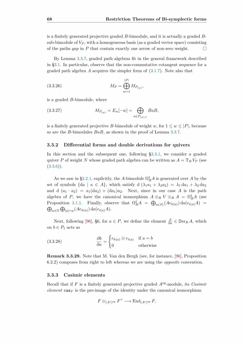
68 Restriction Theorems of Bi-symplectic forms
is a finitely generated projective graded B-bimodule, and it is actually a graded B-sub-bimodule of VP , with a homogeneous basis (as a graded vector space) consistingof the paths qap in P that contain exactly one arrow of non-zero weight.
By Lemma 3.3.7, graded path algebras fit in the general framework describedin §3.1. In particular, observe that the non-commutative cotangent sequence for agraded path algebra A acquires the simpler form of (3.1.7). Note also that
(3.3.26) MP =|P |⊕w=1
MP(w) ,
is a graded B-bimodule, where
(3.3.27) MP(w) = Ew[−w] =⊕
a∈P(w),1
BaB,
is a finitely generated projective B-bimodule of weight w, for 1 ≤ w ≤ |P |, becauseso are the B-bimodules BaB, as shown in the proof of Lemma 3.3.7.
3.3.2 Differential forms and double derivations for quivers
In this section and the subsequent one, following §3.3.1, we consider a gradedquiver P of weight N whose graded path algebra can be written as A = TR VP (see(3.3.6)).
As we saw in §2.2.1, explicitly, the A-bimodule Ω1RA is generated over A by the
set of symbols da | a ∈ A, which satisfy d (λ1a1 + λ2a2) = λ1 da1 + λ2 da2and d (a1 · a2) = a1(da2) + (da1)a2. Next, since in our case A is the pathalgebra of P , we have the canonical isomorphism A ⊗R V ⊗R A = Ω1
RA (seeProposition 3.1.1. Finally, observe that Ω1
RA =⊕
a∈P1(Aeh(a)) da(et(a)A) =⊕
w∈N⊕|a|=w(Aeh(a)) da(et(a)A).
Next, following [96], §6, for a ∈ P , we define the element ∂∂a ∈ DerRA, which
on b ∈ P1 acts as
(3.3.28) ∂b
∂a=eh(a) ⊗ et(a) if a = b
0 otherwise
Remark 3.3.29. Note that M. Van den Bergh (see, for instance, [96], Proposition6.2.2) composes from right to left whereas we are using the opposite convention.
3.3.3 Casimir elements
Recall that if F is a finitely generated projective graded Aop-module, its Casimirelement casF is the pre-image of the identity under the canonical isomorphism
F ⊗(Ae)op F∨ −→ End(Ae)op F,

3.3. Restriction Theorem in weight 1 69
where (following [30], §5.3), given a graded Aop-module, F∨ := HomAe(F,AeAe)
is the graded dual A-bimodule equipped with the graded A-bimodule structureinduced by the outer A-bimodule structure on A ⊗ A. In the following result, wedetermine the Casimir element for a graded quiver:
Lemma 3.3.30. Let P be a graded quiver. Then
casVP =∑a∈P1
a⊗ a
is the element Casimir for the (Re)opQ -module VP , where a ∈ V ∨P is given by
a(b) =eh(a) ⊗ et(a) if a = b
0 otherwise,
for a homogeneous b ∈ P1.
Proof. First, observe that VP is an (Re)opQ -module using (2.1.5). We have to check
that eval(∑
a∈P1a⊗ a
)(b) = b for all homogeneous b ∈ P1. Therefore, recalling
that, by convention, we compose arrows from right to left,
eval
∑a∈P1
a⊗ a
(b) =∑a∈P1
a · a(b) = eh(b) b et(b) = b
The reason that explains our interest in Casimir elements for quivers is that theinverse of the canonical map eval : V ∨P ⊗ReAe −→ HomAe(VP ,AeAe) (see (2.1.25b))is given by(3.3.31)κ : HomAe(VP ,AeAe)→ V ∨P ⊗ReAe : g 7→
∑a∈P1
a⊗g(a) =∑a∈P1
(−1)g′′(a)⊗a⊗g′(a),
where we regard VP as an ReQ-module and we use the isomorphism V ∨P ⊗Re Ae '
A⊗R V ∨P ⊗R A (see Remark 3.1.12), g(a) = g′(a)⊗ (g′′)op(a) ∈ Ae for a ∈ P1 and(−1) = (−1)|g′′(a)|(|g′(a)|+N−|a|).
3.3.4 The bi-symplectic form for a graded double quiver
Duals and biduals
Let P be a double graded quiver of weight N whose graded path algebra will bedenoted by A. Following [30], §8.1, consider a function ε : P −→ ±1 takingε(a) = 1 if a ∈ P and -1 if a ∈ P ∗ := P \ P .
It is familiar that there exist four sensitive ways of defining the dual of anR-bimodule. Nevertheless, as [16] points out, all these can be identified by fixinga trace on R (which is a finite-dimensional semisimple algebra over k), that is, ak-linear map Tr: R −→ k such that the bilinear form R⊗R→ k : (a, b) 7−→ Tr(ab)is symmetric and non-degenerate.

70 Restriction Theorems of Bi-symplectic forms
More precisely, let V be an R-bimodule, V ∗ := Hom(V, k) and V ∨ :=Hom(V,R ⊗ R). Then the function Tr: R → k allows us define an isomorphismB : V ∗ → V ∨ by requiring that for ψ ∈ V ∗ and v ∈ V
ψ(v) = Tr((B(ψ)′)(v)) Tr((B(ψ)′′)(v))
Now we consider the graded A-bimodule VP and the space of linear maps V ∗P
:=Hom(VP , k). Recall that A has a basis aa∈P 1
consisting of all the paths in P solet aa∈P 1
⊂ V ∗Pbe the dual basis. Then, if b ∈ A
a(b) = δab
=
1 if a = b
0 otherwise
= Tr(δabeh(a)) Tr(et(a))= Tr((a)′(b)) Tr((a)′′(b))= Tr
(B(a)′(b)
)Tr(B(a)′′(b)
),
which implies that B(a) = a and, consequently,
(3.3.32) B−1(a) = a
Now, using the function ε(a), we define
〈−,−〉 : VP × VP → k : (a, b) 7→ 〈a, b〉 =ε(a) if a = b∗
0 otherwise=
1 if a = b∗ ∈ P1
−1 if a = b∗ ∈ P ∗10 otherwise
It is not difficult to see that (VP , 〈−,−〉) is a symplectic graded vector spaceof weight N . Moreover, VP has a graded R-bimodule structure and the symplecticform 〈−,−〉 gives an isomorphism of graded R-bimodules. Inspired in [30], definean isomorphism, where VP is regarded as a vector space:
(3.3.33) #: V ∗P
∼=−→ VP [−N ] : a 7−→ ε(a)a∗
The bi-symplectic form on a graded double quiver
Let ω :=∑
a∈P1da da∗ ∈ DR2
RA. Then,
Proposition 3.3.34. The 2-form ω is bi-symplectic of weight N , with N even.
Proof. This result and its proof are graded versions of [30], Proposition 8.1.1(ii).It is clear that dω = 0.To prove the non-degeneracy, the idea is to show thatι(ω) coincides with the composition of the following isomorphisms of graded A-bimodules which we shall construct below:(3.3.35)
DerRA 'H
// A⊗R V ∗P ⊗R A'
Id⊗#⊗Id// A⊗R VP ⊗R A
'G
// Ω1RA

3.3. Restriction Theorem in weight 1 71
Next, using (3.3.31), the isomorphism H will be defined as the followingcomposite:
DerRA G∨ // (A⊗R VP ⊗R A)∨ κ // A⊗R V ∨P ⊗R AId⊗B−1⊗Id // A⊗R V ∗P ⊗R A
where
(A⊗R VP ⊗R A)∨ = HomAe(A⊗R VP ⊗R A,AeAe)A⊗R V ∨P ⊗R A = A⊗R HomRe(VP ,ReRe)⊗R A
A⊗R V ∗P ⊗R A = A⊗R Hom(VP , k)⊗R A
More concretely, if Θ ∈ DerRA:
H(Θ) =((Id⊗B−1 ⊗ Id) κ G∨
)(Θ)
=(Id⊗B−1 ⊗ Id
)∑a∈P 1
(−1)|Θ′′(a)|(|Θ′(a)|+N−|a|)Θ′′(a)⊗ a⊗Θ′(a)
=∑a∈P 1
(−1)|Θ′′(a)|(|Θ′(a)|+N−|a|)Θ′′(a)⊗ a⊗Θ′(a)
In conclusion, if (−1) := (−1)|Θ′′(a)|(|Θ′(a)|+N−|a|),
(3.3.36)H : DerRA
∼=−→ A⊗R V ∗P ⊗R A
Θ 7−→∑a∈P 1
(−1)Θ′′(a)⊗ a⊗Θ′(a)
Using (3.3.33), the isomorphism Id ⊗ # ⊗ Id can be defined in the followingterms :
(3.3.37)Id⊗#⊗ Id : A⊗R V ∗P ⊗R A
∼=−→ A⊗R VP ⊗R A∑a∈P 1
(−1)Θ′′(a)⊗ a⊗Θ′(a) 7−→∑a∈P 1
(−1)Θ′′(a)⊗ ε(a)a∗ ⊗Θ′(a)
Finally, we shall describe the image under the canonical isomorphism wrote inProposition (3.1.1) for the object obtained so far:
(3.3.38)G : A⊗R VP ⊗R A
∼=−→ Ω1RA∑
a∈P 1
(−1)Θ′′(a)⊗ ε(a)a∗ ⊗Θ′(a) 7−→∑a∈P 1
(−1)ε(a)Θ′′(a) da∗Θ′(a)
To finish the proof, we have to check that the element obtained in (3.3.38)coincides with the map DerRA→ Ω1
RA : Θ 7→ ιΘω. Now, by (2.2.11):
(3.3.39)
iΘω = iΘ
∑a∈P1
dada∗
=∑a∈P1
((−1)|Θ||a|iΘ(da) da∗ − da(iΘ(da∗))
)=∑a∈P1
((−1)|Θ||a|Θ′(a)⊗ (Θ′′(a) da∗)− (daΘ′(a∗))⊗Θ′′(a∗)
)

72 Restriction Theorems of Bi-symplectic forms
The last step is to apply (−) (see (2.2.14)) and m (defined in (2.2.15)) to(3.3.39):
ιΘω = m (iΘω)
= m
∑a∈P1
((−1)|Θ||a|Θ′(a)⊗ (Θ′′(a) da∗)− (daΘ′(a∗))⊗Θ′′(a∗)
)
= m (∑a∈P1
(−1)|Θ||a|(−1)|Θ′(a)|(|Θ′′(a)+N−|a|)(Θ′′(a) da∗)⊗Θ′(a)−
− (−1)|Θ′′(a∗)|(|a|+|Θ′(a∗)|)Θ′′(a∗)⊗ (daΘ′(a∗)))
As, by hypothesis, N is even, in the sign of the first summand, we have that|Θ||a|+ |Θ′(a)|(|Θ′′(a) +N − |a|) = |Θ′′(a)|(|Θ′(a) +N − |a|):
=∑a∈P1
((−1)|Θ′′(a)|(|Θ′(a)+N−|a|)Θ′′(a) da∗ Θ′(a)−
− (−1)|Θ′′(a∗)|(|a|+|Θ′(a∗)|)Θ′′(a∗) da Θ′(a∗))
=∑a∈P 1
(−1)ε(a)Θ′′(a) da∗Θ′(a)
3.3.5 Restriction Theorem in weight 1 for double graded quivers
Theorem 3.3.40. Let P be a double graded quiver of weight 2 whose graded pathalgebra shall be denoted by A := kP . Consider R as the semisimple finite dimen-sional algebra with basis the trivial paths in P and let B be the smooth path algebraof the weight 0 subquiver of P .
Assume that A is endowed with a a bi-symplectic form ω ∈ DR2R (A) of weight
2, and that it can be written as A = TBM where M is the graded B-bimodule
M := E1[−1]⊕ E2[−2],
for finitely generated projective B-bimodules E1 and E2. Then the isomorphismι(ω) : DerRA −→ Ω1
RA[−2] restricts, in weight 1, to the B-bimodule isomorphism
(3.3.41) (ι(ω))1 : E∨1∼=−→ E1 : a 7−→ ε(a)a∗,
whose inverse is
(3.3.42) [ : E1∼=−→ E∨1 : a 7−→ ε(a)a∗
Proof. Recall that A can be described as TR VP and TBMP (see (3.3.5) and(3.3.25) respectively), by Lemma 3.3.7 in this subsection, we shall consider thefollowing commutative diagram, where we will use H and G which will be definedin (3.3.50) and (3.3.46), respectively:
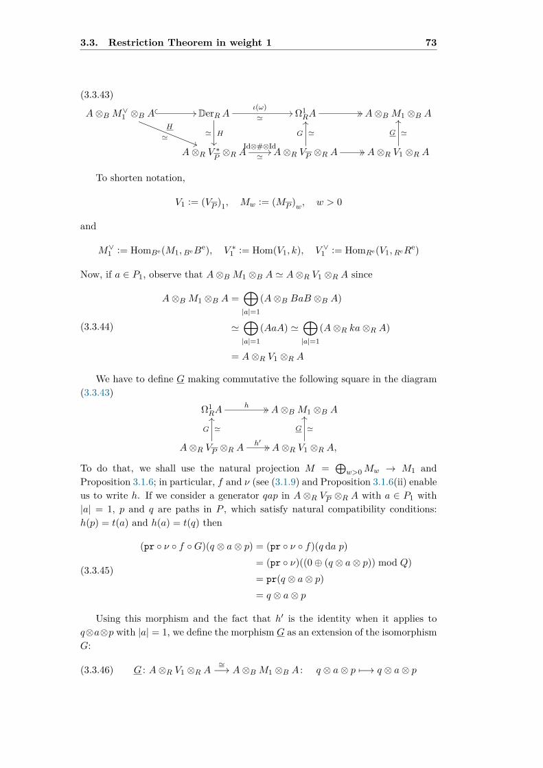
3.3. Restriction Theorem in weight 1 73
(3.3.43)
A⊗B M∨1 ⊗B A //
H
'((
DerRAι(ω)'
//
H'
Ω1RA
// // A⊗B M1 ⊗B A
A⊗R V ∗P ⊗R AId⊗#⊗Id'// A⊗R VP ⊗R A // //
G '
OO
A⊗R V1 ⊗R A
G '
OO
To shorten notation,
V1 := (VP )1, Mw := (MP )w, w > 0
and
M∨1 := HomBe(M1,BeBe), V ∗1 := Hom(V1, k), V ∨1 := HomRe(V1,ReRe)
Now, if a ∈ P1, observe that A⊗B M1 ⊗B A ' A⊗R V1 ⊗R A since
(3.3.44)
A⊗B M1 ⊗B A =⊕|a|=1
(A⊗B BaB ⊗B A)
'⊕|a|=1
(AaA) '⊕|a|=1
(A⊗R ka⊗R A)
= A⊗R V1 ⊗R A
We have to define G making commutative the following square in the diagram(3.3.43)
Ω1RA
h // // A⊗B M1 ⊗B A
A⊗R VP ⊗R Ah′ // //
G '
OO
A⊗R V1 ⊗R A,
G '
OO
To do that, we shall use the natural projection M =⊕
w>0Mw → M1 andProposition 3.1.6; in particular, f and ν (see (3.1.9) and Proposition 3.1.6(ii) enableus to write h. If we consider a generator qap in A ⊗R VP ⊗R A with a ∈ P1 with|a| = 1, p and q are paths in P , which satisfy natural compatibility conditions:h(p) = t(a) and h(a) = t(q) then
(3.3.45)
(pr ν f G)(q ⊗ a⊗ p) = (pr ν f)(q da p)= (pr ν)((0⊕ (q ⊗ a⊗ p)) mod Q)= pr(q ⊗ a⊗ p)= q ⊗ a⊗ p
Using this morphism and the fact that h′ is the identity when it applies toq⊗a⊗p with |a| = 1, we define the morphism G as an extension of the isomorphismG:
(3.3.46) G : A⊗R V1 ⊗R A∼=−→ A⊗B M1 ⊗B A : q ⊗ a⊗ p 7−→ q ⊗ a⊗ p

74 Restriction Theorems of Bi-symplectic forms
Thus, G is an isomorphism.
Now, we define the isomorphism H (obtained from H by restriction). Firstly,in order to obtain
(3.3.47) M∨1 ⊗Re Ae // DerRA,
we observe that if a ∈ P 1 is such that |a| = 1 and a ∈ M∨1 is the correspondingelement in the dual basis, then a⊗1Ae ∈M∨1 ⊗BeAe can be regarded as an elementbelonging to V ∨
P⊗Re Ae by (3.3.44) and the natural injection.. So our task is to
determine an object in DerRA from the element a ⊗ 1Ae ∈ V ∨P⊗Re Ae using the
sequence of isomorphisms
(3.3.48)
V ∨P⊗Re Ae ' HomRe(VP ,HomAe(Ae, Ae))
' HomRe(Ae ⊗Re VP ,AeAe)= HomAe(Ω1
RA,AeAe)= DerRA
which, as A is the graded path algebra of the graded double quiver P , can beexplicitly described in the following way:
• Under the first isomorphism V ∨P⊗Re Ae ' HomRe(VP ,HomAe(Ae, Ae)), we
obtaina⊗ 1Ae 7−→ eval(a⊗ 1Ae)
where (see (2.1.25b))
eval(a⊗ 1Ae) : VP∼=−→ Ae
b 7−→ a(b) ∗ 1Ae
• Under the second isomorphism HomRe(VP ,HomAe(Ae, Ae)) ' HomRe(Ae⊗Re
VP ,AeAe),eval(a⊗ 1Ae) 7−→ f1
given by
f1(b) : Ae ∼=−→ Ae
a1 ⊗ bop1 7−→ (eh(a) ⊗ et(a))(a1 ⊗ bop
1 )
where b ∈ VP .
• Under the third isomorphism in (3.3.48), HomRe(Ae ⊗Re VP ,AeAe) =HomAe(Ω1
RA,AeAe), we write
f1 7−→ f2
where
f2 : Ae ⊗Re VP∼=−→ Ae
(a1 ⊗ bop1 )⊗ b 7−→ (a1 ⊗ bop
1 )(eh(a) ⊗ et(a)) ∗ 1Ae

3.3. Restriction Theorem in weight 1 75
• Finally, under the fourth isomorphism, HomAe(Ae ⊗Re VP , Ae)
∼=−→HomAe(Ω1
RA,AeAe),f2 7−→ i ∂
∂a,
where, using (3.3.28),
i ∂∂a
: Ω1RA −→ Ae
(a1 ⊗ bop1 ) db 7−→ ±(a1eh(a))⊗ (et(a)b1)
To sum up, the previous discussion enables us to determine (3.3.47),
(3.3.49) M∨1 ⊗Be Ae −→ DerRA : a⊗ 1Ae 7−→ ∂
∂a,
where ∂∂a ∈ DerRA was defined in (3.3.28). Now, following (3.3.43), we apply the
isomorphism H:
H
(∂
∂a
)=(Id⊗B−1 ⊗ Id
)(et(a) ⊗ a⊗ eh(a))
= et(a) ⊗ a⊗ eh(a)
Therefore, we are able to write H:
(3.3.50)H : M∨1 ⊗Be Ae −→ A⊗R V ∗P ⊗R A
a⊗ 1Ae 7−→ et(a) ⊗ a⊗ eh(a),
Again in the diagram (3.3.43), we use the isomorphism Id⊗#⊗ Id (see (3.3.37)):
(3.3.51)Id⊗#⊗ Id : A⊗R V ∗P ⊗R A −→ A⊗R VP ⊗R A
et(a) ⊗ a⊗ eh(a) 7−→ et(a) ⊗ ε(a)a∗ ⊗ eh(a)
Finally, to construct an element in A ⊗B M1 ⊗B A from (3.3.51), we apply h′
and G (which were defined in (3.3.45) and (3.3.46), respectively) to obtain theelement
et(a) ⊗ ε(a)a∗ ⊗ eh(a) = 1⊗ ε(a)a∗ ⊗ 1 ∈ A⊗B M1 ⊗B A.
Using (3.3.43), we were able to construct an isomorphism between A⊗BM∨1 ⊗BA and A⊗BM1⊗B A given by 1⊗ a⊗ 1 7→ 1⊗ ε(a)a∗⊗ 1. If (−)1 denotes the partof weight 1, (A⊗BM∨1 ⊗BA)1 = B⊗BM∨1 ⊗BA 'M∨1 because, by hypothesis, thedouble graded quiver has weight 2. Similarly, (A⊗B M1 ⊗B A) ' M1. Therefore,we obtain the following isomorphism of B-bimodules:
(3.3.52) R : E∨1∼=−→ E1 : a 7−→ ε(a)a∗,
whose inverse is
(3.3.53) [ : E1∼=−→ E∨1 : a 7−→ ε(a)a∗


Chapter 4
Bi-symplectic NQ-algebras of weight 1
D. Roytenberg [81] proved that symplectic NQ-manifolds of weight 1 are in 1-1correspondence with ordinary Poisson manifolds. In this chapter, we extend thisresult to the non-commutative setting. Once we review Roytenberg’s result in §4.1,we carry out the classification of bi-symplectic tensor N-algebras of weight 1 (see§4.2), which are in 1-1 correspondence with smooth associative algebras. In thelast section of the chapter, we introduce the essential notion of bi-symplectic NQ-algebras (which can be regarded as the non-commutative analogues of symplecticNQ-manifolds) and in Theorem 4.3.2 we classify them in weight 1: bi-symplecticNQ-algebras of weight 1 are in 1-1 correspondence with double Poisson algebras.
4.1 Symplectic NQ-manifolds of weight 1
In this subsection we will review the classification of symplectic NQ-manifoldscarried out by D. Roytenberg in [81], Proposition 4.1, which states that symplecticNQ-manifolds of weight 1 are in 1-1 correspondence with ordinary Poissonmanifolds.
4.1.1 Basics on symplectic polynomial N-algebras
Recall that an N-graded manifold (an N-manifold, for short)M of weight n and di-mension (p; r1, ..., rn) is a smooth p-dimensional manifold M endowed with a sheafC∞(M) of N-graded commutative associative unital R-algebras, which can locallybe written as C∞U (M)[ξ1
1 , ..., ξr11 , ξ
12 , ..., ξ
r22 , ..., ξ
1n, ..., ξ
rnn ] with ξji of weight i and U
is an open subset of M . An NQ-manifold (M, Q) is an N-manifold endowed withan integrable homological vector field Q of weight +1 (i.e. [Q,Q] = 2Q2 = 0).A symplectic NQ-manifold (M, ω,Q) is an NQ-manifold whose homological vectorfield is compatible with ω in the sense that LQω = 0, where LQ stands for the Liederivative along the vector field Q.
In graded geometry, it is crucial that every N-manifold comes equipped with
77

78 Bi-symplectic NQ-algebras of weight 1
the graded Euler vector field:
(4.1.1) Eu =n∑i=1|xi|xi ∂
∂xi,
where xini=1 are the coordinates of the N–manifolds and |xi| denotes the weightof xi or, equivalently, it is the derivation which acts on homogeneous smooth func-tions via E(f) = |f |f . Consequently, the weights are just the eigenvalues withrespect to the action of Eu in (4.1.1).
The Euler vector field Eu acts on all canonical objects (tensors, jets,...) onMby means of the Lie derivative. As a consequence, these objects acquire weights. Inparticular, following [81], we are interested in homogeneous symplectic and Poissonstructures; a symplectic structure of weight k is a closed non-degenerate 2-form ω
such that LEuω = kω, where LEu denotes the Lie derivative along the Euler vectorfield Eu.
The space of all homogeneous functions of weight k will be denoted by Ak. Thegraded algebra
A =⊕k≥0
Ak,
is the algebra of polynomial functions on the N-manifold. Observe that the algebraof all smooth functions is a completion of A and the weight of the N-manifold isby definition the highest weight of a local coordinate.
In this section, let R be a commutative k-algebra, where k is a field of char-acteristic zero. A commutative R-algebra is a commutative k-algebra B equippedwith a unit preserving k-algebra embedding R → B. A commutative B-algebra isthen a commutative R-algebra A endowed with an algebra homomorphism B → A
compatible with the identity map R → R (in particular, it is unit preserving).Also, observe that the definition of Z-graded commutative B-algebra is containedin §2.1, adding the hypothesis of commutativity:
Definition 4.1.2. Let B a commutative R-algebra.
(i) A commutative N-algebra over B (shorthand for ‘non-negatively gradedalgebra’) is a Z-graded commutative B-algebra A such that Ai = 0 for alli < 0. We say a ∈ A is homogeneous of weight |a| = i if a ∈ Ai.
(ii) A polynomial N-algebra over B is a commutative N-algebra A over B whichcan be written as a symmetric graded algebra A = Sym•BM , for a positivelygraded B-module M , so M =
⊕i∈ZM
i, where M i = 0 for i ≤ 0.
(iii) We say m ∈M is homogeneous of weight |m| = i if m ∈M i.
(iv) The weight of a commutative N-algebra A is |A| := minS∈G
maxa∈S|a|, where the
elements of G are the finite sets of homogeneous generators of A.

4.1. Symplectic NQ-manifolds of weight 1 79
Next, we define one of the central objects of this section:
Definition 4.1.3 (Symplectic polynomial algebra of weight N). Let A be apolynomial N-algebra. An element ω ∈ Ω2
RA is a symplectic form of weight Nif it has the following properties:
(i) ω is closed for the universal derivation d ,
(ii) ω is homogeneous of weight N (i.e. LEuω = Nω),
(iii) The map of graded A-modules is an isomorphism:
i(ω) : DerRA −→ Ω1RA[−N ] : θ 7−→ iθω.
A polynomial N-algebra over B equipped with a symplectic form of weight N isa symplectic polynomial N-algebra of weight N over B if in the decompositionA = Sym•BM withM a graded B-bimodule, M i = 0 for i > N andM j is a finitelygenerated projective B-module for 0 ≤ j ≤ N .
It is well-known that if ω ∈ Ω2RA is a symplectic form of weight N , define the
Hamiltonian vector field Ha ∈ DerRA corresponding to a homogenous a ∈ A via
(4.1.4) ιHaω = da,
and write
(4.1.5) a, bω = Ha(b) ∈ A
Moreover, following [20], recall that a derivation X ∈ DerRA is calledsymplectic if the Lie derivative of ω with respect to X vanishes, i.e. LXω = 0.Symplectic structures of weight k 6= 0 impose strong constrains on symplecticpolynomial N-algebras as the following result shows:
Lemma 4.1.6 ([81], Lemma 2.2). Let A be a symplectic polynomial N-algebra overB. Then
(i) Any homogeneous symplectic form ω on A of weight k 6= 0 is exact.
(ii) Any homogeneous derivation X ∈ DerRA of weight l < −k preserving ω isHamiltonian.
Proof. Both results are applications of Cartan’s identity. Since ω is a symplecticform of weight k 6= 0, LEuω = kω and dω = 0:
kω = LEuω = diEuω,
and we conclude (i). By definition,
0 = LXω = diXω.
Taking H := iEuiXω, we use Cartan’s identity:
dH = diEuiXω. = LEu(iXω) = (m+ n)iXω.
and (ii) holds.

80 Bi-symplectic NQ-algebras of weight 1
Since Ha(b) = iHa(db), (4.1.5) can be written in the following form:
(4.1.7) a, bω = ιHaιHbω.
The essential point is that (A, −,−ω) has a very remarkable structure:
Definition 4.1.8 (Poisson algebra of weight −N , [54]). Let A be a gradedcommutative algebra. We will call A a Poisson algebra of weight −N if it isequipped with a graded bilinear map (called the Poisson bracket of weight −N),
−,− : A⊗A −→ A
of weight −N such that the following identities hold:
(i) (Graded anti-symmetry)
(4.1.9) a, b = −(−1)(|a|−N)(|b|−N)b, a,
(ii) (Graded Leibniz)
(4.1.10) a, bc = a, bc+ (−1)(|a|−N)|b|ba, c,
(iii) (Graded Jacobi)
(4.1.11) a, b, c = a, b, c+ (−1)(|a|−N)|b|b, a, c.
Lemma 4.1.12. If (A,ω) is a symplectic polynomial N-algebra of weight N , then(A, −,−ω) in (4.1.7) is a Poisson algebra of weight −N on A.
Proof. In order to determine the weight of −,−ω, observe that by (4.1.4),|Ha|+ |ω| = |a| and by (4.1.5), |a, bω| = |a|+ |b|− |ω|. Thus, −,−ω = −N .
4.1.2 Classification of symplectic polynomial N-algebras
Let B a smooth commutative R-algebra and (A,ω) a symplectic polynomial N-algebra of weight 1.
By (4.1.7) and Lemma 4.1.12, ω, the symplectic form of weight 1 induces−,−ω, a Poisson bracket of weight −1 on A which is determined by the followinginclusions
(4.1.13) A0, A0ω = 0, A1, A0ω ⊂ A0, A1, A1ω ⊂ A1,
Proposition 4.1.14 ([81], Proposition 3.1). Symplectic polynomial N-algebras ofweight 1 are in 1-1 correspondence, up to isomorphism, with ordinary smoothcommutative algebras, via B ↔ (DerRB,Ω), where Ω is determined by thecommutator of derivations on B.

4.1. Symplectic NQ-manifolds of weight 1 81
Proof. Let (A,ω) be a symplectic polynomial N-algebra of weight 1. By definition,the weight of A cannot exceed |ω| = 1 hence A = Sym•BM , where B = A0 andM = A1 = E[−1] for a finitely generated projective B-module E.
By (4.1.13), A1, A0ω ⊂ A0, and we can define the following action of theB-module A1 = M [−1] on A0 = B is meaningful
ρ : A1 −→ HomR(B,B) : a 7−→ (Ha = a,−ω : B −→ B)
As −,−ω is a Poisson bracket, Ha satisfies
Ha(bb′) = a, bb′ω = ba, b′ω + a, bωb′ = bHa(b′) +Ha(b)b′,
for all b, b′ ∈ B, so Ha ∈ DerRB and the map ρ : A1 → DerRB[−1] is anisomorphism by the non-degeneracy of −,−ω. By (4.1.11), we have the followingidentity:
Xa1,a2ω(b) = a1, a2ω, bω= − (b, a1ω, a2ω + a1, b, a2ωω)= a1, a2, bωω − a2, a1, bωω= [Xa1 , Xa2 ](b),
where [−,−] denotes the commutator of derivations on B. Thus, under theisomorphism ρ, the Poisson bracket on A1 corresponds to the commutator ofderivations on B.
4.1.3 Classification of symplectic polynomial NQ-algebras ofweight 1
This subsection is devoted to prove, in an algebraic formulation, Roytenberg’sclassification of symplectic polynomial NQ-algebras:
Definition 4.1.15. (i) A commutative NQ-algebra over B (A,Q) is a commu-tative N-algebra A over B endowed with a derivation Q : A → A of weight+1 which is homological, i.e. such that [Q,Q] = 0, where [−,−] is the gradedcommutator of derivations.
(ii) A polynomial NQ-algebra over B is a commutative NQ-algebra over B whoseunderlying commutative N-algebra is a polynomial N-algebra over B.
(iii) A symplectic NQ-algebra over B of weight N (A,Q, ω) is a polynomial NQ-algebra endowed with a symplectic form ω ∈ Ω2
RA of weight N such that
(a) The underlying polynomial N-algebra is a symplectic polynomial N-algebra of weight N over B, and
(b) the homological derivation Q is symplectic.

82 Bi-symplectic NQ-algebras of weight 1
Theorem 4.1.16 ([81], Theorem 4.1). Symplectic NQ-algebras of weight 1 are in1-1 correspondence with Poisson algebras.
Proof. Let R be a commutative k-algebra, where k is a field of characteristiczero, and B a smooth commutative R-algebra. Let (A,Q, ω) be a symplectic NQ-algebra of weight 1. In particular, Q is a symplectic homological derivation, thatis, LQω = 0 and [Q,Q] = 0. By Lemma 4.1.6(ii), we write
Q = HS = S,−ω,
where S ∈ A and −,−ω is the Poisson bracket of weight -1 induced by ω
on A. In fact, by definition, Q has weight +1 and the identity for all b ∈ B
Θ, bω = HΘ(b) = Q(b) yields
|S| = |Q| − |−,−ω| = 2.
Thus S ∈ A2. Crucially, in Proposition 4.1.14 we established an isomorphism ofGerstenhaber algebras (A, −,−ω) ∼= (
∧B DerRB, [−,−]), where, as usual, [−,−]
stands for the Schouten bracket of multi-vector fields. This isomorphism preservesweights so, as S is a Hamiltonian quadratic function over A, it corresponds underthis isomorphism to an element P ∈
∧2B DerRB.
By the graded Jacobi identity (4.1.11), we have the identity Ha,bω = [Ha, Hb]which applied to a = b = S gives
HS,Sω = [Q,Q]
Therefore, if a ∈ A,
[Q,Q](a) = HS,Sω(a) = S, Sω, aω,
and the relation [Q,Q] = 0 is equivalent to S, Sω ∈ B because the equation(4.1.4) provides S, Sω ∈ R but B is a commutative R-algebra. However,S, Sω has weight 3 because |S| = 2. Therefore, we conclude that S, Sω = 0.Furthermore, the isomorphism ρ exchanges appropriately the brackets −,−ω and[−,−], so S, Sω = 0 implies that [P, P ] = 0, that is, P is a Poisson bivector, asrequired.
4.2 Classification of bi-symplectic tensor N-algebras ofweight 1
From now on, R is a finite dimensional semisimple k-algebra, where k is a field ofcharacteristic zero, and B is a smooth associative R-algebra.
Theorem 4.2.1. Bi-symplectic tensor smooth N-algebras of weight 1 are in 1-1 correspondence, up to isomorphism, with smooth associative R-algebras. The

4.3. Classification of bi-symplectic NQ-algebras of weight 1 83
correspondence assigns to each smooth associative R-algebra B, the pair (A,ω)consisting of the tensor N-algebra
A = T∗[1]B := TB(DerRB[−1])
and the bi-symplectic form ω determined by the double Schouten–Nijenhuis bracketof the tensor algebra of the B-bimodule of double derivations over B.
Proof. Let (A,ω) be a bi-symplectic tensor N-algebra of weight 1. By definition,the weight of A cannot exceed |ω| = 1. Hence A = TBM , where B = A0 andM = A1 = E[−1] for a finitely generated projective B-bimodule E. Observe that,under these hypothesis, A is a smooth algebra (see Proposition 2.2.23).
Define a double Poisson bracket on A by a, bω = Ha(b) (2.5.4), whereHa ∈ DerRA is the Hamiltonian double derivation corresponding to a ∈ A. Thisdouble Poisson bracket is non-degenerate, because ω is bi-symplectic, and hasweight -1, since |ω| = 1, so it satisfies
A0, A0ω
= 0,A1, A0
ω⊂ (A⊗A)0,
A1, A1
ω⊂ (A⊗A)1.
By the second identity, we can define the following action of the bimoduleA1 = M [−1] on A0 = B, which is meaningful:
ρ : A1 −→ HomRe(B,B ⊗B) : a 7−→ (Ha = a,−ω : B −→ B ⊗B)
As −,−ω is a double Poisson bracket, Ha satisfies
Ha(fg) = a, fgω = f a, gω + a, fω g = fHa(g) +Ha(f)g,
for all f, g ∈ B, so Ha ∈ DerRB and the map ρ : A1 → DerRB[−1] is an isomor-phism, by Theorem 3.2.2.
Now, Proposition 2.4.6 establishes that ρ(a, bω) = Ha,bω = Ha, Hb =ρ(a), ρ(b), where −,− is the canonical double Schouten–Nijenhuis bracketon TB DerRB. Thus, under the isomorphism ρ, the double Poisson bracket onA1 corresponds to the double Schouten–Nijenhuis bracket on the noncommutativecotangent bundle TB DerRB on B.
4.3 Classification of bi-symplectic NQ-algebras ofweight 1
Definition 4.3.1. (i) An associative NQ-algebra (A,Q) over B is an associativeN-algebra A of weight N over B endowed with a double derivation Q : A →A⊗ A of weight +1 which is homological, i.e. such that Q,Q = 0, where−,− stands for the double Schouten-Nijenhuis bracket.
(ii) A tensor NQ-algebra (A,Q) is an associative NQ-algebra over B whoseunderlying associative N-algebra is a tensor N-algebra over B.

84 Bi-symplectic NQ-algebras of weight 1
(iii) A bi-symplectic NQ-algebra of weight N (A,ω,Q) is a tensor NQ-algebra overB endowed with a bi-symplectic form ω ∈ DR2
R (A) of weight N such that
(a) The underlying tensor N-algebra over B is a bi-symplectic tensor N-algebra of weight N over B, and
(b) the homological double derivation Q is bi-symplectic.
By Proposition 2.3.20, if (A,P ) is a differential double Poisson algebra (DDPfor short –recall §2.3.3), then A is a double Poisson algebra with double Poissonbracket −,−P . Therefore, for a smooth algebra A, the notions of DDP algebraand double Poisson algebra are equivalent. The following result is the main resultof this chapter because it is the non-commutative analogue of [81], Theorem 4.1:
Theorem 4.3.2. Bi-symplectic NQ-algebras of weight 1 are in 1-1 correspondence,up to isomorphism, with double Poisson algebras.
Proof. Let (A,ω,Q) be a bi-symplectic NQ-algebra of weight 1. In particular,Q is a bi-symplectic homological double derivation, that is, LQω = 0 andQ,Q = 0, where −,− denotes the double Schouten–Nijenhuis bracket. ByLemma 2.5.6(ii), we write
Q = S,−ω ,
where S ∈ A and −,−ω is the weight -1 double Poisson bracket induced by thebi-symplectic form ω on A. In fact, by definition, |Q| = +1 and the identity (see(2.4.3))
S, aω = HS(a) = Q(a)
for all a ∈ A yields|S| = |Q| − |−,−ω| = 2.
Thus, S ∈ A2. Next, by Proposition 4.2.1, the bi-symplectic tensor N-algebra (A,ω) is isomorphic to the noncommutative cotangent bundle. In otherwords, we have an isomorphism of double Gerstenhaber algebras (A, −,−ω) ∼=(TB DerRB, −,−). This isomorphism preserves weights so, as S is a Hamil-tonian quadratic function over A, it corresponds under this isomorphism to anelement P ∈ (TB DerRB)2, a two-fold of the tensor algebra of DerRB over B.
Now, the identityHa,bω = Ha, Hb given by Proposition 2.4.6, which appliesto a = b = S, gives
HS,Sω = Q,Q .
Therefore, if a ∈ A,
Q,Q (a) = HS,Sω(a) = S, Sω , aω .
Now, the relation Q,Q = 0 is equivalent to Θ,Θω ∈ B⊗B because, by (2.4.2),HΘ,Θω = 0 implies that 0 = dΘ,Θω = dΘ,Θ′ω ⊗ Θ,Θ
′′ω + Θ,Θ′ω ⊗
dΘ,Θ′′ω, which implies that Θ,Θ′ω , Θ,Θ′′ω ∈ R. Finally, since B is an asso-
ciative R-algebra, we conclude that Θ,Θ′ω , Θ,Θ′′ω ∈ B as we required and, as
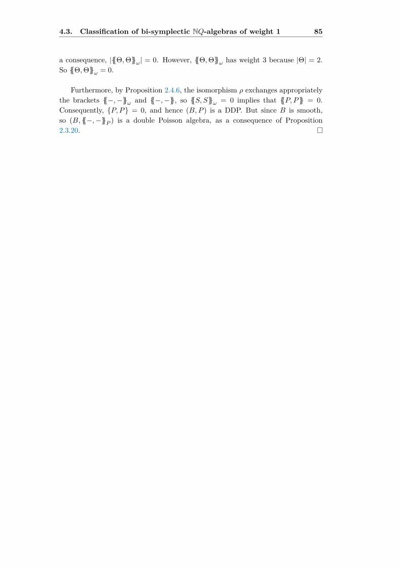
4.3. Classification of bi-symplectic NQ-algebras of weight 1 85
a consequence, |Θ,Θω| = 0. However, Θ,Θω has weight 3 because |Θ| = 2.So Θ,Θω = 0.
Furthermore, by Proposition 2.4.6, the isomorphism ρ exchanges appropriatelythe brackets −,−ω and −,−, so S, Sω = 0 implies that P, P = 0.Consequently, P, P = 0, and hence (B,P ) is a DDP. But since B is smooth,so (B, −,−P ) is a double Poisson algebra, as a consequence of Proposition2.3.20.


Chapter 5
Bi-symplectic tensor N-algebras ofweight 2
Chapter 5 is somehow the core of this thesis. In §5.1 we sketch a result of D.Roytenberg that can be reformulated more algebraically using Lie–Rinehart al-gebras (the algebraic structure corresponding to Lie algebroids) as follows: thestructure of a symplectic polynomial N-algebra of weight 2 is completely deter-mined by a finitely generated projective B-module E1 endowed with a symmetricnon-degenerate bilinear form 〈−,−〉 (see [81], Theorem 3.3). In §5.2, if B is asmooth associative algebra, given a bi-symplectic tensor N-algebra of weight 2 overB A = TB(E1[−1] ⊕ E2[−2] where E1 and E2 are projective finitely generatedB-bimodules, we calculate A0, A1 and A2, the subspaces Aw ⊂ A of weights 0,1,2,and determine the structure of the double Poisson bracket of weight -2 induced bythe bi-symplectic form. §5.4 is devoted to define a non-commutative counterpartof a Lie–Rinehart algebra (see Definition 5.4.1) and to prove in Proposition 5.4.9that A2 has this structure.
A key point in our discussion is that E1 is endowed with a pairing (in the senseof [97], §3.1), whose definition is reviewed in (5.3.3). Using the results of §3.3,we construct a non-degenerate symmetric pairing for double graded quivers (seeLemma 5.3.7). In §5.3.4, we prove that this pairing is compatible, in a suitablesense (see §5.3.4), with certain family of “double covariant differential operators”Da introduced in §5.3.2.
In §5.5 we introduce the notion of double Atiyah algebra and metric doubleAtiyah algebra At(E1) which are endowed with brackets (5.5.8), resembling Vanden Bergh’s double Schouten–Nijenhuis bracket. In Proposition 5.5.10 we provethat At(E1) is a double Lie–Rinehart algebra. Finally, §5.6 is devoted to prove thata map Ψ: A2 → At(E1), defined in (5.6.2) using the “double covariant differentialoperators”, is a map of twisted double Lie–Rinehart algebras (see Proposition5.6.1). Furthermore, in §5.7 we demonstrate that, in the setting of double gradedquivers, Ψ is an isomorphism and, consequently, we conclude that our bi-symplectictensor N-algebra A over B of weight 2 is completely determined by E1 together
87
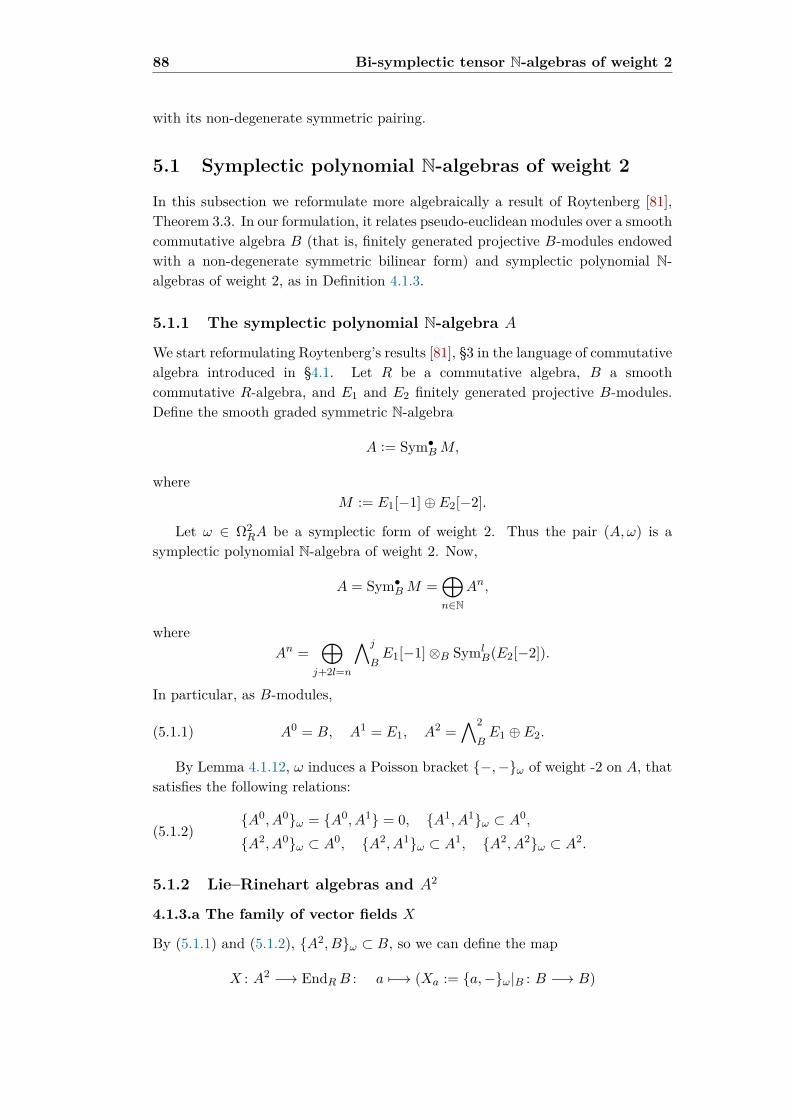
88 Bi-symplectic tensor N-algebras of weight 2
with its non-degenerate symmetric pairing.
5.1 Symplectic polynomial N-algebras of weight 2
In this subsection we reformulate more algebraically a result of Roytenberg [81],Theorem 3.3. In our formulation, it relates pseudo-euclidean modules over a smoothcommutative algebra B (that is, finitely generated projective B-modules endowedwith a non-degenerate symmetric bilinear form) and symplectic polynomial N-algebras of weight 2, as in Definition 4.1.3.
5.1.1 The symplectic polynomial N-algebra A
We start reformulating Roytenberg’s results [81], §3 in the language of commutativealgebra introduced in §4.1. Let R be a commutative algebra, B a smoothcommutative R-algebra, and E1 and E2 finitely generated projective B-modules.Define the smooth graded symmetric N-algebra
A := Sym•BM,
whereM := E1[−1]⊕ E2[−2].
Let ω ∈ Ω2RA be a symplectic form of weight 2. Thus the pair (A,ω) is a
symplectic polynomial N-algebra of weight 2. Now,
A = Sym•BM =⊕n∈N
An,
whereAn =
⊕j+2l=n
∧j
BE1[−1]⊗B Syml
B(E2[−2]).
In particular, as B-modules,
(5.1.1) A0 = B, A1 = E1, A2 =∧2
BE1 ⊕ E2.
By Lemma 4.1.12, ω induces a Poisson bracket −,−ω of weight -2 on A, thatsatisfies the following relations:
(5.1.2)A0, A0ω = A0, A1 = 0, A1, A1ω ⊂ A0,
A2, A0ω ⊂ A0, A2, A1ω ⊂ A1, A2, A2ω ⊂ A2.
5.1.2 Lie–Rinehart algebras and A2
4.1.3.a The family of vector fields X
By (5.1.1) and (5.1.2), A2, Bω ⊂ B, so we can define the map
X : A2 −→ EndRB : a 7−→ (Xa := a,−ω|B : B −→ B)

5.1. Symplectic polynomial N-algebras of weight 2 89
Since −,−ω is a Poisson bracket, in particular, it satisfies the graded Leibnizrule (4.1.10) in its second argument, so
Xa(b1b2) = a, b1b2ω = b1Xa(b2) +Xa(b1)b2,
for all a ∈ A2, b1, b2 ∈ B. In other words, Xa ∈ DerRB, so the map X can be seenas a “family of vector fields” parametrized by A2, i.e. a map
(5.1.3) X : A2 −→ DerRB : a 7−→ (Xa := a,−ω|B : B −→ B) .
4.1.3.b Lie–Rinehart algebras
For sake of completeness, we recall now the definition of Lie–Rinehart algebra (see,for example, [83], Definition B.1):
Definition 5.1.4 (Lie–Rinehart algebra). Let k be a field of characteristic 0, R acommutative k-algebra and B a commutative R-algebra. A Lie–Rinehart algebraover B consists of the following data:
(i) A B-module L;
(ii) A B-module map ρ : L −→ DerRB, called the anchor ;
(iii) A R-bilinear Lie bracket −,−L : L⊗ L→ L.
These data are required to satisfy the following additional conditions:
(a) a1, ba2L = ba1, a2L + ρ(a1)(b)a2;
(b) ρ(a1, a2L) = [ρ(a1), ρ(a2)],
for all a1, a2 ∈ L, b ∈ B, and where [−,−] denotes the commutator of derivations.
Observe that in (iii), we follow our convention (see §2.1) that all unadornedtensor products are over the base field k. Moreover, the Lie bracket is skew-symmetric and it satisfies the Jacobi identity.
Definition 5.1.5. Let (L, ρL, −,−L), (L′, ρL′ , −,−L′) be Lie–Rinehart alge-bras. We say that ϕ : L → L′ is a map of Lie–Rinehart algebras if it preservesbrackets:
ϕ(−,−L) = ϕ(−), ϕ(−)L′ .
Example 5.1.6. The prototypical example of Lie–Rinehart algebra is DerRB withrespect to the commutator bracket [−,−] and the identity map DerRB → DerRBas the anchor. As Roytenberg points out in [83], Lie–Rinehart algebras form acategory and DerRB is the terminal object of the category.

90 Bi-symplectic tensor N-algebras of weight 2
4.1.3.b A2 as a Lie–Rinehart algebra
Proposition 5.1.7. A2 is a Lie–Rinehart algebra, with the bracket
−,− := −,−ω|A2⊗A2 : A2 ⊗A2 −→ A2,
and the anchor given by the map X : A2 → DerRB in (5.1.3).
Proof. First of all, the bracket is well-defined, because A2, A2ω ⊂ A2 by (5.1.2).Then we have to heck conditions (a) and (b) of Definition 5.1.4. The proof is basedon the fact that (A, −,−ω) is a Poisson algebra of weight -2
Condition (a) follows because by the graded Leibniz rule (recall Definition4.1.8):
a1, ba2 = ba1, a2ω + a1, bωa2 = ba1, a2+ ρ(a1)(b)a2
for all a1, a2 ∈ A and b ∈ B. Similarly, condition (b) follows because by the gradedJacobi identity (4.1.11), given b ∈ B,
ρ(a1, a2)(b′) = a1, a2ω, b′ω= −
(b′, a1, a2ωω + a1, b′, a2ωω
)= a1, a2, b
′ωω − a2, a1, b′ωω
= [ρ(a1), ρ(a2)](b′)
5.1.3 The inner product
4.1.4.a The family of covariant differential operators D
By (5.1.2), we have the relation A2, A1ω ⊂ A1 , so we can consider
(5.1.8) D : A2 −→ EndRE1 : a 7−→ (Da := a,−ω|E1 : E1 −→ E1) .
Observe that this map and X in (5.1.3) are closely related to each other as aconsequence of the (graded) Leibniz rule:
Da(be) = bDa(e) +Xa(b)e
for all a ∈ A2, e ∈ E1, and b ∈ B. We point out that the pair (X,D) is a derivationin the sense of [83] or a covariant differential operator as was defined in [60].
4.1.4.b The inner product
By (5.1.1) and the inclusion A1, A1ω ⊂ A0 in (5.1.2), we can define
〈−,−〉 := −,−ω|E1⊗E1 : E1 ⊗ E1 → B
In [81], Roytenberg claims the following result:
Lemma 5.1.9. 〈−,−〉 is a non-degenerate symmetric B-bilinear form over E1.
〈−,−〉 will called an inner product.

5.1. Symplectic polynomial N-algebras of weight 2 91
4.1.4.c The preservation of the inner product
The map D in (5.1.8) preserves the inner product 〈−,−〉 in the sense that
(5.1.10) Xa(〈e1, e2〉) = 〈Da(e1), e2〉+ 〈e1, Da(e2)〉
for all a ∈ A2 and e1, e2 ∈ E1. This follows by (4.1.11):
(5.1.11)
Xa(〈e1, e2〉) = a, e1, e2ωω= a, e1ω, e2ω + e1, a, e2ωω= Da(e1), e2ω + e1, Da(e2)ω= 〈Da(e1), e2〉+ 〈e1, Da(e2)〉
5.1.4 The Atiyah algebra
4.1.5.a Definition of Atiyah algebra
We will use the following algebraic formulation of Atiyah algebroid (see e.g. [51],§2.2, [52], (1.1.3) Example (c) for non-metric variants).
Definition 5.1.12. We define the metric Atiyah algebra, At(E1) as the set of pairs(X,D), where X ∈ DerRB and D ∈ EndRE1 are such that, for all b ∈ B, ande, e1, e2 ∈ E1,
(i) D(be) = bD(e) +X(b)e;
(ii) X(〈e1, e2〉) = 〈D(e1), e2〉+ 〈e1, D(e2)〉.
4.1.5.b The Atiyah algebra as a Lie–Rinehart algebra
Proposition 5.1.13. At(E1) is a Lie–Rinehart algebra, with bracket given by
[(X1, D1), (X2, D2)]At := ([X1, X2], [D1, D2]),
For all (X1, D1), (X2, D2) ∈ At(E1),where [X1, X2] denotes the commutator ofderivations, and anchor
ρ : At(E1) −→ DerRB : (X,D) 7−→ X.
Proof. Note that [(X1, D1), (X2, D2)]At ∈ At(E1), because
[D1, D2](be) = D1(D2)(be)−D2(D1)(be)= D1(bD2(e) +X2(b)e)−D2(bD1(e) +X1(b)e)= b(D1(D2(e))−D2(D1(e))) + (X1(X2(b))−X2(X1(b)))e= b[D1, D2](e) + [X1, X2](b)e

92 Bi-symplectic tensor N-algebras of weight 2
and
[X1, X2]〈e1, e2〉 = X1 (X2〈e1, e2〉)−X2 (X1〈e1, e2〉)= X1 (〈D2(e1), e2〉+ 〈e1, D2(e2)〉)−−X2 (〈D1(e1), e2〉+ 〈e1, D1(e2)〉)= 〈D1(D2(e1)), e2〉+ 〈e1, D1(D2(e2))〉−− 〈D2(D1(e1)), e2〉 − 〈e1, D2(D1(e2))〉= 〈[D1, D2](e1), e2〉+ 〈e1, [D1, D2](e2)〉
Condition (a) of Definition 5.1.4 now follows because D1(be) = bD1(e) +ρ(X1, D1)(b)e for e ∈ E and b ∈ B, so
[D1, bD2](e) = D1(bD2(e))− b(D2(D1(e)))= bD1(D2(e)) +D1(b)D2(e)− bD2(D1(e))= (b(D1 D2 −D2 D1) +X1(b)D2)(e)= b[D1, D2](e) +X1(b)D2(e)
Finally, condition (b) of Definition 5.1.4 is a direct consequence of the definitionof the anchor:
ρ([(X1, D1), (X2, D2)]At) = ρ([X1, X2], [D1, D2])= [X1, X2]= [ρ(X1, D1), ρ(X2, D2)]
5.1.5 The map ψ
By Proposition 5.1.7 and Proposition 5.1.13, we showed that A2 and At(E1) areLie–Rinehart algebras. This section is devoted to prove that
Proposition 5.1.14.
(5.1.15)ψ : A2 −→ At(E1)
a 7−→ (Xa, Da)
is a map of Lie–Rinehart algebras.
Lemma 5.1.16. For all a1, a2 ∈ A2,
(i) Xa1,a2 = [Xa1 , Xa2 ],
(ii) Da1,a2 = [Da1 , Da2 ].
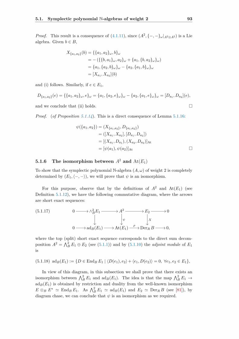
5.1. Symplectic polynomial N-algebras of weight 2 93
Proof. This result is a consequence of (4.1.11), since (A2, −,−ω|A2⊗A2) is a Liealgebra. Given b ∈ B,
Xa1,a2(b) = a1, a2ω, bω= − (b, a1ω, a2ω + a1, b, a2ωω)= a1, a2, bωω − a2, a1, bωω= [Xa1 , Xa2 ](b)
and (i) follows. Similarly, if e ∈ E1,
Da1,a2(e) = a1, a2ω, eω = a1, a2, eωω − a2, a1, eωω = [Da1 , Da2 ](e),
and we conclude that (ii) holds.
Proof. (of Proposition 5.1.14). This is a direct consequence of Lemma 5.1.16:
ψ(a1, a2) = (Xa1,a2, Da1,a2)= ([Xa1 , Xa2 ], [Da1 , Da2 ])= [(Xa1 , Da1), (Xa2 , Da2)]At
= [ψ(a1), ψ(a2)]At
5.1.6 The isomorphism between A2 and At(E1)
To show that the symplectic polynomial N-algebra (A,ω) of weight 2 is completelydetermined by (E1, 〈−,−〉), we will prove that ψ is an isomorphism.
For this purpose, observe that by the definitions of A2 and At(E1) (seeDefinition 5.1.12), we have the following commutative diagram, where the arrowsare short exact sequences:
(5.1.17) 0 // ∧2BE1 //
A2 //
ψ
E2 //
X
0
0 // adB(E1) // At(E1) ρ// DerRB // 0,
where the top (split) short exact sequence corresponds to the direct sum decom-position A2 =
∧2B E1 ⊕ E2 (see (5.1.1)) and by (5.1.10) the adjoint module of E1
is
(5.1.18) adB(E1) := D ∈ EndB E1 | 〈D(e1), e2〉+ 〈e1, D(e2)〉 = 0, ∀e1, e2 ∈ E1,
In view of this diagram, in this subsection we shall prove that there exists anisomorphism between
∧2B E1 and adB(E1). The idea is that the map
∧2B E1 →
adB(E1) is obtained by restriction and duality from the well-known isomorphismE ⊗B E∗ ' EndB E1. As
∧2B E1 ' adB(E1) and E2 ' DerRB (see [81]), by
diagram chase, we can conclude that ψ is an isomorphism as we required.
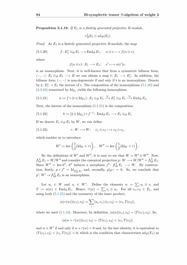
94 Bi-symplectic tensor N-algebras of weight 2
Proposition 5.1.19. If E1 is a finitely generated projective B-module,
∧2BE1 ' adB(E1)
Proof. As E1 is a finitely generated projective B-module, the map
(5.1.20) f : E∗1 ⊗B E1 −→ EndB E1 : α⊗ e 7−→ f(α⊗ e),
wheref(α⊗ e) : E1 −→ E1 : e′ 7−→ α(e′)e.
is an isomorphism. Next, it is well-known that from a symmetric bilinear form,〈−,−〉 : E1 ⊗B E1 −→ B we can obtain a map [ : E1 −→ E∗1 . In addition, thebilinear form 〈−,−〉 is non-degenerate if and only if [ is an isomorphism. Denoteby ] : E∗1 → E1 the inverse of [. The composition of the isomorphisms (5.1.20) and(3.3.42) tensorized by IdE1 yields the following isomorphism:
(5.1.21) a := f ([⊗ IdE1) : E1 ⊗B E1∼=−→ E∗1 ⊗B E1
∼=−→ EndB E1,
Next, the inverse of the isomorphism (5.1.21) is the composition:
(5.1.22) b := (]⊗ IdE1) f−1 : EndB E1 −→ E1 ⊗B E1
If we denote E1 ⊗B E1 by W , we can define
(5.1.23) τ : W −→W : e1 ⊗ e2 7−→ e2 ⊗ e1,
which enables us to introduce
W ′ := ker(
12(IdW + τ)
), W ′′ := ker
(12(IdW + τ)
).
By the definitions of W ′ and W ′′, it is easy to see that W = W ′ ⊕W ′′. Now,∧2B E1 = W/W ′′ and consider the canonical projection p : W −→W/W ′′ =
∧2B E1.
Since W ′′ = kerh′′, h′′ induces a morphism j′′ :∧2B E1 −→ W . By construc-
tion, firstly, p j′′ = Id∧2B E1
and, secondly, p|W ′′ = 0. So, we conclude thatp′ : W ′ →
∧2B E1 is an isomorphism.
Let ui ∈ W and vi ∈ W ∗. Define the elements w =∑
i ui ⊗ vi andT := a(w) ∈ EndB E1. Hence, τ(w) =
∑i vi ⊗ ui. For all e1, e2 ∈ E1, and
using both (5.1.21) and the symmetry of the inner product,
〈a(τ(w))(e1), e2〉 =∑i
〈ui, e1〉〈vi, e2〉 = 〈e1, T (e2)〉,
where we used (5.1.18). Moreover, by definition, 〈a(w)(e1), e2〉 = 〈T (e1), e2〉. So,
〈a(w + τ(w))(e1), e2〉 = 〈T (e1), e2〉+ 〈e1, T (e2)〉
and w ∈W ′ if and only if w+ τ(w) = 0 and, by the last identity, it is equivalent to〈T (e1), e2〉+ 〈e1, T (e2)〉 = 0, which is the condition that characterizes adB(E1) as
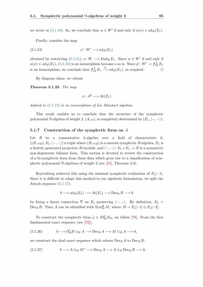
5.1. Symplectic polynomial N-algebras of weight 2 95
we wrote in (5.1.18). So, we conclude that w ∈W ′ if and only if a(w) ∈ adB(E1).
Finally, consider the map
(5.1.24) a′ : W ′ −→ adB(E1)
obtained by restricting (5.1.21), a : W −→ EndB E1. Since w ∈ W ′ if and only ifa(w) ∈ adB(E1), (5.1.24) is an isomorphism because a so is. Since p′ : W ′ →
∧2B E1
is an isomorphism, we conclude that∧2B E1
∼=−→ adB(E1), as required.
By diagram chase, we obtain
Theorem 5.1.25. The map
ψ : A2 −→ At(E1)
defined in (5.1.15) is an isomorphism of Lie–Rinehart algebras.
This result enables us to conclude that the structure of the symplecticpolynomial N-algebra of weight 2, (A,ω), is completely determined by (E1, 〈−,−〉).
5.1.7 Construction of the symplectic form on A
Let R be a commutative k-algebra over a field of characteristic 0,((B,ωB), E1, 〈−,−〉) a triple where (B,ωB) is a smooth symplectic R-algebra, E1 isa finitely generated projective B-module, and 〈−,−〉 : E1×E1 → B is a symmetricnon-degenerate bilinear form. This section is devoted to review the constructionof a bi-symplectic form from these data which gives rise to a classification of sym-plectic polynomial N-algebras of weight 2 (see [81], Theorem 3.3).
Roytenberg achieved this using the minimal symplectic realization of E1[−1].Since it is difficult to adapt this method to our algebraic formulation, we split theAtiyah sequence (5.1.17):
0 −→ adB(E1) −→ At(E1) −→ DerRB −→ 0
by fixing a linear connection ∇ on E1 preserving 〈−,−〉. By definition, E2 =DerRB. Then A can be identified with Sym•BM , where M = E1[−1]⊕ E2[−2].
To construct the symplectic form ω ∈ (Ω2RA)2, we follow [79]. From the first
fundamental exact sequence (see [72]),
(5.1.26) 0 −→ Ω1RB ⊗B A −→ DerRA −→M ⊗B A −→ 0,
we construct the dual exact sequence which relates DerRA to DerRB:
(5.1.27) 0 −→ A⊗B M∗ −→ DerRA −→ A⊗B DerRB −→ 0,

96 Bi-symplectic tensor N-algebras of weight 2
where M∗ := HomB(M,B). Using the connection ∇ we can split this short exactsequence
(5.1.28) DerRA ' A⊗B (M∗ ⊕DerRB)
By (5.1.28), to construct the symplectic form ω ∈ (Ω2RA)2 or, equivalently,
i(ω) : DerRA → Ω1RA[−2], we can specify its value iφ+∇X on φ +∇X ∈ DerRA,
where φ ∈ M∗, X ∈ DerRB. As A = Sym•BM is a smooth algebra becauseB is a smooth R-algebra and M is a finitely generated projective B-module,Ω1RA ' HomA(DerRA,A). Then,
iφ+∇X ω : DerRA −→ A
ψ +∇Y 7−→ eval(iφ+∇X ω, ψ +∇Y ),
where eval(−,−) denotes the usual pairing between one-forms and derivations.Hence, in order to define ω, it is enough to determine ω(φ, ψ), ω(∇X ,∇Y ) andω(∇X , ψ) for φ, ψ ∈M∗ and X,Y ∈ DerRB. Nevertheless, it is easy to check thatω(φ, ψ) = 0 unless that φ, ψ ∈ E∗1 (for instance, if φ1 ∈ E∗1 and φ2 ∈ E∗2 thenω(φ1, φ2) = A−1 = 0). The 2-form ω ∈ (Ω2
RA)2 is defined by
ω(∇X ,∇Y ) = ωB(X,Y ) + 12R(X,Y )(5.1.29)
ω(φ, ψ) = 〈φ, ψ〉,(5.1.30)ω(∇X , φ) = 0,(5.1.31)
where R denotes the contraction of the curvature R of ∇ with the inner product〈−,−〉. In [79], Theorem 1, M. Rothstein proved that ω is a symplectic form.Finally, observe that, by (5.1.30), we have the identity
e1, e2ω = 〈e1, e2〉
for all e1, e2 ∈ E1.
5.2 The algebra A
Let R be a semisimple associative k-algebra, where k is a field of characteristiczero, and B a smooth associative R-algebra. Let E1 and E2 be projective finitelygenerated B-bimodules. Define the smooth graded tensor N-algebra:
A := TBM,
of the graded B-bimodule
M := E1[−1]⊕ E2[−2],
where the notation Ei[−i] was introduced in §2.1 Let ω ∈ DR2R (A) be a bi-
symplectic form of weight 2. Thus the pair (A,ω) is a bi-symplectic tensor N-algebra of weight 2 (see Definition 3.2.1). Then
A =⊕n∈N
An,

5.3. The pairing 97
whereAn =
⊕n∈N
⊕j+2l=n
(E1[−1]⊗Bj ⊗ E2[−2]⊗B l
).
In particular,
(5.2.1) A0 = B, A1 = E1, A2 = (E1 ⊗B E1)⊕ E2.
By (2.5.4) and Lemma 2.5.5, the bi-symplectic form ω on A determines adouble Poisson bracket of weight -2, denoted by −,−ω. This bracket satisfiesthe following relations:
(5.2.2)
A0, A0
ω=A0, A1
ω= 0,
A1, A1ω⊂ (A⊗A)0 = B ⊗B,
A2, A0ω⊂ (A⊗A)0 = B ⊗B,
A2, A1ω⊂ (A⊗A)1 = (E1 ⊗B)⊕ (B ⊗ E1),
A2, A2ω⊂ (A⊗A)2.
5.3 The pairing
5.3.1 The family of double derivations X
By (5.2.1) and (5.2.2),A2, B
ω⊂ B ⊗B, so we can define the map
(5.3.1) X : A2 −→ HomRe(B,BeBe) : a 7−→ (Xa := a,−ω |B : B −→ B ⊗B) .
Since −,−ω is a double Poisson bracket of weight -2, it satisfies the gradedLeibniz rule (2.3.10) in its second argument (with respect to the outer structure),and so
Xa(b1b2) = a, b1b2ω = b1 a, b2ω + a, b1ω b2 = b1Xa(b2) + Xa(b1)b2,
for all a ∈ A2, and b1, b2 ∈ B. Therefore Xa ∈ DerRB, so X can be seen as a“family of double derivations” parametrized by A2, i.e. it is a map
(5.3.2)X : A2 −→ DerRB
a 7−→ Xa := a,−ω |B : B −→ B ⊗B.
5.3.2 The family of double differential operators D
By (5.2.2),A2, A1
ω⊂ (A ⊗ A)1 = (E1 ⊗ B) ⊕ (B ⊗ E1), so we can define the
following map:
(5.3.3)D : A2 −→ HomRe(E1, E1 ⊗B ⊕B ⊗ E)
a 7−→ Da := a,−ω |E1
By the graded Leibniz rule (2.3.10) applied to −,−ω,
Da(be) = bDa(e) + Xa(b)e,(5.3.4a)Da(eb) = Da(e)b+ eXa(b),(5.3.4b)
for all a ∈ A2, e ∈ E1, b ∈ B; so D can be seen as a ‘family of double differentialoperators’.

98 Bi-symplectic tensor N-algebras of weight 2
5.3.3 The pairing
Given an arbitrary associative k-algebra C, Van den Bergh [97], §3.1, defines apairing between two C-bimodules P and Q as a map
〈−,−〉 : P ×Q→ C ⊗ C,
such that 〈p,−〉 is linear for the outer bimodule structure on C ⊗ C and 〈−, q〉is linear for the inner bimodule structure on C ⊗ C, for all p ∈ P , q ∈ Q. Wesay that the pairing is non-degenerate if P and Q are finitely generated projectiveC-bimodules and the pairing induces an isomorphism
Q∼=−→ P∨ : q 7−→ 〈−, q〉,
where, as usual, (−)∨ stands for HomCe(−, CeCe) (see §2.1.1)).
Using the third inclusion in (5.2.2), we define
〈−,−〉 := −,−ω |(E1⊗E1) : E1 ⊗ E1 → B ⊗B
Recall that a double bracket, in particular, is a double derivation in its secondargument for the outer bimodule structure on B ⊗B and, correspondingly, it is adouble derivation in its first argument for the inner bimodule structure on B⊗B.Therefore, since 〈−,−〉 is the restriction of −,−ω to E1⊗E1, is immediate that〈−,−〉 is a pairing. Moreover, for all e1, e2 ∈ E1,
〈e1, e2〉 = e1, e2ω |(E1⊗E1) = σ(12) e2, e1ω |(E1⊗E1) = σ(12)〈e2, e1〉
where we used (2.3.11) and |e1| = |e2| = 1. Thus we can conclude that 〈−,−〉 issymmetric.
To prove that this pairing is non-degenerate, we will restrict to the set-up ofdouble graded quivers given in §3.3.
(5.3.5) [ : E1 −→ E∨1 : a 7→ ε(a)a∗.
We define the following map:
(5.3.6)〈−,−〉 : E1 ⊗ E1 −→ B ⊗B
(a, b) 7−→ [(a)(b) = ε(a)a∗(b).
Now, we can compute a, bω = i ∂∂aι ∂∂bω, using the tools developed in §3.3,
where a, b ∈ P are arrows of weight 1, ∂∂a ,
∂∂a ∈ DerRA (see (3.3.28)) and ω is the

5.3. The pairing 99
symplectic form of Proposition 3.3.34:
a, bω = i ∂∂aι ∂∂bω
= i ∂∂a
∑a∈P 1
ε(b∗)eh(b)(db)et(b)
=∑a∈P 1
i ∂∂a∗
(ε(b∗)eh(b)(db)et(b))
= ε(a)a∗(b)= 〈a, b〉.
Therefore, we have the following result:
Lemma 5.3.7. The map 〈−,−〉 : E1 × E1 → B ⊗ B defined in (5.3.6) is anon-degenerate symmetric pairing between E1 and itself and coincides with therestriction to E1 ⊗ E1 of −,−ω.
Proof. It is clear that 〈−,−〉 is a pairing. Now, if a, b are arrows of weight 1,σ(12)〈a, b〉 = ε(b)et(b)⊗eh(b) = 〈b, a〉. Finally, the non-degeneration is a consequenceof Theorem 3.3.40.
5.3.4 The preservation of the pairing
Since Da ∈ (A ⊗ A)1 for all a ∈ A2, it is useful to extend the pairing (5.3.6) to amap
〈−,−〉L : E1 × (A⊗A)1 −→ (A⊗A)1
by
(5.3.8) 〈e, e′ ⊗ b〉L = 〈e, e′〉 ⊗ b, 〈e, b⊗ e′〉L = 0,
for all e, e′ ∈ E1 and b ∈ B, where we have used (A ⊗ A)1 = E1 ⊗ B ⊕ B ⊗ E1.Then the map D preserves the pairing in the sense that
(5.3.9) σ(123)Xa(〈e2, e1〉) = 〈e1,Da(e2)〉L + σ(132)〈e2,Da(e1)〉L,
where the map Xa in (5.3.2) is extended to A ⊗ A using the Leibniz rule. Thisfollows from the graded double Jacobi identity:
〈e1,Da(e2)〉L = e1, a, e2ωω,L= σ(123) a, e2, e1ωω,L + σ(132) e2, e1, aωω,L= σ(123) a, e2, e1ωω,L − σ(132)
e2, σ(12) a, e1ω
ω,L
= σ(123)Xa(〈e2, e1〉)− σ(132)〈e2,Da(e1)〉.

100 Bi-symplectic tensor N-algebras of weight 2
5.4 A2 and twisted double Lie–Rinehart algebras
5.4.1 Definition of twisted double Lie–Rinehart algebras
According to Van den Bergh’s Definition 3.2.1 in [97], a double Lie algebroid over Ais an A-bimodule L with a double Poisson bracket of weight -1 on TA L. However,this definition has two drawbacks for our purposes; firstly, there is no referenceto the anchor map, and, secondly, it only considers double Poisson brackets ofweight -1. To have a suitable definition of double Lie–Rinehart algebra in ournon-commutative setting, we should require the following:
(i) (A2, −,−ω ,X) should have this algebraic structure.
(ii) The “double Atiyah algebroid” should be a double Lie–Rinehart algebra.
(iii) We would like to adapt the method of the proof of [96], Proposition 3.5.1, toshow a non-commutative version of Proposition 5.1.14 in §5.1.5.
Definition 5.4.1 (Twisted double Lie–Rinehart algebra). Let R be a semisimpleassociative k-algebra over a field of characteristic zero, and B be an associativeR-algebra. A twisted double Lie–Rinehart algebra over B consists of the followingdata:
(i) A B-bimodule N ;
(ii) A B-subbimodule N ⊂ N endowed with a symmetric non-degenerate pairing,〈−,−〉N , called the appendix;
(iii) A B-bimodule map ρ : N → DerRB, called the anchor ;
(iv) A R-bilinear bracket
−,−N : N ⊗N −→ N ⊗B ⊕B ⊗N ⊕N ⊗N,
called the double bracket. These data are required to satisfy the following additionalconditions:
(a) a1, a2N = −σ(12) a2, a1N
(b) a1, ba2N = b a1, a2N + ρ(a1)(b)a2
(c) a1, a2bN = a1, a2N b+ a2ρ(a1)(b)
(d)
0 = a1, a2, a3NN,L + σ(123) a2, a3, a1NN,L +
+ σ(132) a3, a1, a2NN,L
(e) ρ(a1, a2N ) = ρ(a1), ρ(a2)SN.

5.4. A2 and twisted double Lie–Rinehart algebras 101
where a1, a2, a3 ∈ N , b ∈ B, −,−SN denotes the double Schouten–Nijenhuisbracket (see (2.3.14)). Finally, observe that all products involved are with respectto the outer bimodule structure, and ρ acts by the Leibniz rule on tensor products.
If the appendix is zero, we say that N is a double Lie–Rinehart algebra.
Remark 5.4.2. Following [96], §2.3, if x′ ∈ TB N and x = x1⊗· · ·⊗xn ∈ (TB N)nthen we define
x′, xN,L
=x′, x1
N⊗ x2 ⊗ · · · ⊗ xn.
Example 5.4.3. Using [96], Theorem 3.2.2, it is easy to see that DerRB is adouble Lie–Rinehart algebra with respect to the double Schouten–Nijenhuis bracket−,−SN, the identity map DerRB −→ DerRB as the anchor, and the zero asappendix.
Observe that a1, a2N decomposes as
(5.4.4) a1, a2l′
N⊗a1, a2l′′
N+a1, a2r′
N⊗a1, a2r′′
N +a1, a2m′
N ⊗a1, a2m′′
N ,
where
a1, a2l′
N , a1, a2r′′
N ∈ N, a1, a2r′
N , a1, a2l′′′
N ∈ B,
a1, a2m′
N , a1, a2m′′
N ∈ N.
Now, as by hypothesis, the appendix N is endowed with a non-degeneratesymmetric pairing, we can define the map
(5.4.5) T : N −→ HomBe(N,B ⊗B) : n1 7−→ Tn1 = 〈n1,−〉.
Definition 5.4.6. Let (N, −,−N , ρN ) and (N ′, −,−N ′ , ρN ′) be doubletwisted Lie–Rinehart algebras. We say that ϕ : N → N ′ is a map of twisted doubleLie–Rinehart algebras if satisfies
(5.4.7) ϕ(a1, a2N ) = ϕ(a1), ϕ(a2)N ′
for all a1, a2 ∈ N . Then, by convention, in the left-hand side, we extend the mapof twisted double Lie–Rinehart algebra in the following way:
ϕ(a1, a2N ) = ϕ(a1, a2l′
N )⊗ a1, a2l′′
N + Ta1,a2m′
N⊗ a1, a2m
′′
N +
+ a1, a2m′
N ⊗ Ta1,a2m′′
N+ a1, a2r
′
N ⊗ ϕ(a1, a2r′′
N ).
5.4.2 A2 as a twisted double Lie–Rinehart algebra
As we showed in (5.2.2),A2, A2
ω⊂ (A⊗A)2 ⊂ A⊗A, so we can define
(5.4.8) −,−A2 := −,−ω |A2⊗A2 : A2 ⊗A2 −→ (A⊗A)2.

102 Bi-symplectic tensor N-algebras of weight 2
Proposition 5.4.9. A2 is a double Lie-Rinehart algebra, with the bracket−,−A2, the anchor X : A2 → DerRB, and the appendix given by (E1, 〈−,−〉.
Proof. We have to check that the conditions (a) - (e) in Definition 5.4.1 hold. (b)is an easy consequence of the graded Leibniz rule:
a1, ba2A2 = b a1, a2ω + a1, bω a2
= b a1, a2ω + Xa1(b)a2
= b a1, a2A2 + ρ(a1)(b)a2
for all a1, a2 ∈ A2, b ∈ B. Similarly, we check (c).
Next, since −,−A2 is the restriction of −,−ω to A2 ⊗ A2, and(A, −,−ω) is a double Poisson algebra of weight -2, in particular, the Jacobiidentity in (d) holds. By the same reason, we prove (a).
Finally, the compatibility in (e) is an application of Proposition 2.4.6 because,(A, −,−ω) is a double Poisson bracket of weight -2.
5.5 The Double Atiyah algebra
5.5.1 The definition of double Atiyah algebra
To simplify the notation, we will write
(5.5.1) EndRe(E1) := HomRe(E1, (E1 ⊗B)⊕ (B ⊗ E1)).
If e ∈ E and D ∈ EndRe(E1), we will use the following decomposition:
(5.5.2) D(e) = Dl(e) + Dr(e) = Dl′(e)⊗ Dl
′′(e) + Dr′(e)⊗ Dr
′′(e),
where Dl(e) ∈ E1 ⊗B, Dr(e) ∈ B ⊗ E1 (we omit summation symbols), with
Dl′(e),Dr′′(e) ∈ E1, Dl
′′(e),Dr′(e) ∈ B.
By (5.3.4), we can introduce the following concept:
Definition 5.5.3 (Double Atiyah algebra). Let E be a B-bimodule. We define thedouble Atiyah algebra as the set of pairs (X,D) with X ∈ DerRB and D ∈ EndRe(E)such that,
(i) D(be) = bD(e) + X(b)e,
(ii) D(eb) = D(e)b+ eX(b),
for all b ∈ B, and e ∈ E.
Since the (projective finitely generated) B-bimodule E1 is also equipped witha symmetric non-degenerate pairing 〈−,−〉, constructed in §5.3.3, we shoulddistinguish those double Atiyah algebras which preserve the pairing (see (5.3.9)):

5.5. The Double Atiyah algebra 103
Definition 5.5.4 (Metric double Atiyah algebra). Let (E, 〈−,−〉) be a B-bimoduleequipped with a symmetric non-degenerate pairing. We define At(E), the metricdouble Atiyah algebra of E1, as the double Atiyah algebra which, in addition,preserves the pairing in the sense
σ(123)X(〈e2, e1〉) = 〈e1,D(e2)〉L + σ(132)〈e2,D(e1)〉L,
for all e1, e2 ∈ E, a ∈ A2, X ∈ DerRB and D ∈ EndRe(E).
5.5.2 The bracket
The following construction of a double bracket on A is inspired by Van den Bergh’s[96], §.3.2, double Schouten–Nijenhuis bracket, which is a non-commutative versionof the standard Lie bracket of vector fields. From now on, (X1,D1), (X2,D2) ∈At(E1). To define a bracket between double differential operators, we will usedecomposition (5.5.2):
D1,D2∼l := (Dl1 ⊗ 1B)Dl2 + (X1 ⊗ 1E1)Dr2 −(
(1E1 ⊗ X2)Dl1 + (1B ⊗ Dr2)Dr1)
= Dl1(Dl′2 )⊗ Dl′′
2 + X1(Dr′2 )⊗ Dr′′
2 −(Dl′
1 ⊗ X2(Dl′′1 ) + Dr′
1 ⊗ Dr2(Dr′′1 )),
D1,D2∼r := (1B ⊗ Dr1)Dr2 + (1E1 ⊗ X1)Dl2 −(
(X2 ⊗ 1E1)Dr1 + (Dl2 ⊗ 1B)Dl1)
= Dr′
2 ⊗ Dr1(Dr′′2 ) + Dl′
2 ⊗ X1(Dl′′2 )−(X2(Dr′1 )⊗ Dr
′′1 + Dl2(Dl′1 )⊗ Dl
′′1
),
Note that D1,D2∼l and D1,D2∼r depend on X1 and X2, but we omit thisdependence to simplify the notation. It is immediate that
D1,D2∼l = −D2,D1∼r ,
and
D1,D2∼l (e), D1,D2∼r (e) ∈ (E1 ⊗B ⊗B)⊕ (B ⊗ E1 ⊗B)⊕ (B ⊗B ⊗ E1),
for all e ∈ E1.
Following [96], §3.2, we will regard D1,D2∼l and D1,D2∼r as elements ofEndRe(E1) ⊗ B and B ⊗ EndRe(E1) respectively. More precisely, we define newbrackets:
(5.5.5)D1,D2l = τ(23) D1,D2∼l ,D1,D2r = τ(12) D1,D2∼r ,
where τ(23) and τ(12) are permutations which act on tensor products of the formE1 ⊗B ⊗B, B ⊗ E1 ⊗B, and B ⊗B ⊗ E1. For instance,
τ(23) : E1 ⊗B ⊗B −→ E1 ⊗B ⊗B : e⊗ b1 ⊗ b2 7−→ e⊗ b2 ⊗ b1,τ(23) : E1 ⊗B ⊗B −→ B ⊗ E1 ⊗B : e⊗ b1 ⊗ b2 7−→ b1 ⊗ e⊗ b2.

104 Bi-symplectic tensor N-algebras of weight 2
These new brackets can be decomposed as
(5.5.6)D1,D2l = D1,D2′l ⊗ D1,D2′′lD1,D2r = D1,D2′r ⊗ D1,D2′′r ,
where D1,D2′l , D1,D2′′r ∈ EndRe(E1) and D1,D2′′l , D1,D2′r ∈ B. Again,observe that D1,D2l and D1,D2r depend on X1 and X2, but we omit thisdependence to simplify the notation.
Lemma 5.5.7.D1,D2r = −D2,D1l .
Proof. This result is an easy consequence of the identity D1,D2∼l =−D2,D1∼r and the application of the permutation σ(12) as in [96], (3.2).
Finally, for all b1, b2 ∈ B, X1 ∈ DerRB and D1,D2 ∈ EndRe(E1), we define
(5.5.8)b1, b2 = 0,D1, b1 = X1(b1),D1,D2 = D1,D2l + D1,D2r ,
where, as before, to simplify the notation we omit the dependence of D1,D2 onX1 and X2, and we consider the right-hand sides as elements of (TB EndRe(E1))⊗2.Then the bracket between double differential operators is the unique extension
−,− : (TB EndRe(E1))⊗2 → (TB EndRe(E1))⊗2
of (5.5.8) of weight -1 to the tensor algebra TB EndRe(E1) satisfying the Leibnizrule.
Finally, by (5.5.8), we define the following natural bracket which acts onelements of At(E1):
(5.5.9) [(X1,D1), (X2,D2)]At = (X1,X2SN , D1,D2),
where −,−SN denotes the double Schouten–Nijenhuis bracket. It will be calledthe double Atiyah bracket.
5.5.3 The double Atiyah algebra as a double Lie–Rinehart algebra
Proposition 5.5.10. At(E1) is a double Lie–Rinehart algebra with the bracketgiven by the double Atiyah bracket (5.5.9) and anchor
ρ : At(E1) −→ DerRB : (X,D) 7−→ X.

5.6. The map Ψ 105
Proof. Our proof is partially based on the proof of Theorem 3.2.2 in [96].Condition (a) of Definition 5.4.1 is an easy consequence of Lemma 5.5.7 and [96](3.4). Next, for all b ∈ B and e ∈ E1, we have identities such as
bD2(e) = b(Dl′
2 (e)⊗ Dl′′
2 (e) + Dr′
2 (e)⊗ Dr′′
2
)(e)
= Dl′
2 (e)⊗ bDl′′2 (e) + Dr′
2 (e)⊗ bDr′′2 (e).
Then
D1, bD2r (e) = τ(12) D1, bD2∼r (e)
= τ(12)((1⊗ b · ⊗1)(D1,D2∼r (e) + Dl′
2 (e)⊗ X1(b)Dl′′2 (e)+
+ Dr′
2 (e)⊗ X1(b)Dr′′2 (e)))= (b · ⊗1⊗ 1) D1,D2r (e) + X1(b)D2(e)= b D1,D2r (e) + ρ(X1,D1)(b) D2(e),
and
D1, bD2l (e) = τ(23) D1, bD2∼l (e)= τ(23)((1⊗ 1⊗ b·) D1,D2∼l (e)= (1⊗ b · ⊗1) D1,D2l (e)= b D1,D2l (e).
This implies condition (b) of Definition 5.4.1. The proof of condition (iii) is similar.The Jacobi identity in (d) can be proven by copying (3.7.1) in [96], because we havethe decomposition (5.5.6) and the definition (5.5.8) corresponds to the definitionof the double Schouten–Nijenhuis bracket. Finally, (e) is a consequence of thedefinition of ρ:
ρ([(X1,D1), (X2,D2)]At) = ρ(X1,X2SN , D1,D2)= X1,X2SN
= ρ(X1,D1), ρ(X2,D2)SN
5.6 The map Ψ
Proposition 5.6.1. The map
(5.6.2) Ψ: A2 −→ At(E1)a 7−→ (Xa,Da),
is a map of twisted double Lie–Rinehart algebras.
Proof. We will partially adapt [96], Proposition 3.5.1. We need to prove that
(5.6.3) Ψ(a1, a2A2) = [Ψ(a1),Ψ(a2)]At(E1),

106 Bi-symplectic tensor N-algebras of weight 2
for all a1, a2 ∈ A2, by Definition 5.4.6. More precisely, if we denote −,−A2 by−,−, we have to prove the following identities:
Xa1,a2 = Xa1 ,Xa2 ,(5.6.4a)Da1,a2 = Da1 ,Da2 .(5.6.4b)
Observe that since a1, a2 ∈ (A ⊗ A)2, we can apply the conventions devel-oped in §5.4.1 (in particular, (5.4.4) and (5.4.5)) and, in this way, the left-handsides of (5.6.4) are meaningful.
As (A, −,−ω) is a double Poisson algebra of weight -2, (5.6.4a) is aconsequence of Proposition 2.4.6. To prove (5.6.4b), we will use the double Jacobiidentity(5.6.5)
0 = a1, a2, eωω,L + τ(123) a2, e, a1ωω,L + τ(132) e, a1, a2A2ω,L ,
where e ∈ E1 ⊂ A. By (5.5.2), the first summand in (5.6.5) is
a1, a2, eωω,L = a1,Da2(e)ω,L=a1,Dl
′a2(e)
ω⊗ Dl
′′a2(e) +
a1,Dr
′a2(e)
ω⊗ Dr
′′a2 (e)
= (Da1 ⊗ 1B)Dla2(e) + (Xa1 ⊗ 1E1)Dra2(e),
and the second summand is
a2, e, a1ωω,L = −a2, (Da1(e))ω,L= −
(a2,Dl
′′a1(e)
ω⊗ Dl
′a1(e) +
a2,Dr
′′a1 (e)
ω⊗ Dr
′a1(e)
)= −
((Xa2 ⊗ 1E1)(Dla1(e)) + (Da2 ⊗ 1B)(Dra1(e))
).
Consequently,
τ(123) a2, e, a1ωω,L = −τ(123)(((Xa2 ⊗ 1E1)σ(12)Dla1 + (Da2 ⊗ 1B)σ(12)Dra1)(e))
= −τ(123)τ(132)
((Dl′a1 ⊗ Xa2(Dl′′a1) + Dr
′a1 ⊗ Da2(Dr′′a1
)(e))
= −(
(1E1 ⊗ Xa2)Dla1(e) + (1B ⊗ Da2)Dra1(e)).
Next, we calculate the third summand; combining (5.4.5) and (??),
e, a1, a2A2ω,L =
= −(a1, a2l
′, eω⊗ a1, a2l
′′+a1, a2m
′, eω⊗ a1, a2m
′′),
= −((
Da1,a2l′ (e))⊗ a1, a2l
′′+(Ta1,a2m
′ (e))⊗ a1, a2m
′′),
where we used the fact that a1, a2r′∈ B and, consequently,
e, a1, a2r
′
= 0because −,− is a double Poisson bracket of weight -2. Finally, since τ(12) andτ(23) act on triple tensors (e.g. E1 ⊗B ⊗B),
τ(132) e, a1, a2L =

5.7. The isomorphism between A2 and At(E1) 107
= −τ(132)τ(12)
(Da1,a2l
′ (e)⊗ a1, a2l′′
+ Ta1,a2m′ (e)⊗ a1, a2m
′′)
= −τ(23)
(Da1,a2l
′ (e)⊗ a1, a2l′′
+ Ta1,a2m′ (e)⊗ a1, a2m
′′).
Combining the previous expressions, we obtain(5.6.6)0 = a1, a2, eωω,L + τ(123) a2, e, a1ωω,L + τ(132) e, a1, a2A2ω,L ,
= Da1 ,Da2∼l − τ(23)(Da1,a2l
′ (e)⊗ a1, a2l′′
+ Ta1,a2m′ (e)⊗ a1, a2m
′′)
= Da1 ,Da2l (e)−(Da1,a2l
′ (e)⊗ a1, a2l′′
+ Ta1,a2m′ (e)⊗ a1, a2m
′′).
Finally, by Lemma 5.5.7, we get
(5.6.7)
−a2, a1l′′⊗ Da2,a1l
′ (e) = −a2, a1l′′⊗a2, a1l
′, eω
= −a2, a1l
′′⊗ a2, a1l
′, eω,R
= a1, a2 , eω,R= a1, a2r
′⊗a1, a2r
′′, eω
= a1, a2r′⊗ Da1,a2r
′′ (e)
and, similarly,
(5.6.8) − a2, a1m′′⊗ Ta2,a1m
′ (e) = a1, a2m′⊗ Ta1,a2m
′′ (e)
Thus, by (5.6.6), (5.6.7) and (5.6.8),(5.6.9)Da1 ,Da2r = −Da2 ,Da1
l
= −σ(12)
(Da2,a1l
′ (e)⊗ a2, a1l′′
+ Ta2,a1m′ (e)⊗ a2, a1m
′′)
= −(a2, a1l
′′⊗ Da2,a1l
′ (e) + a2, a1m′′⊗ Ta2,a1m
′ (e))
= a1, a2r′⊗ Da1,a2r
′′ (e) + a1, a2m′⊗ Ta1,a2m
′′ (e)
Finally, (5.6.4b) is the sum of (5.6.6) and (5.6.9), as required
5.7 The isomorphism between A2 and At(E1)
This subsection is devoted to prove that the map Ψ of twisted double Lie–Rinehartalgebras (see Proposition 5.6.1) is an isomorphism, in the setting of double gradedquivers considered in Proposition 3.3.34. In particular, this will imply the proof ofthe following non-commutative version of Roytenberg’s result [81], Theorem 3.3:
Theorem 5.7.1. Let (A,ω) be the pair consisting of the graded path algebra of adouble quiver P of weight 2, and the bi-symplectic form ω ∈ DR2
R (A) of weight2 defined in §3.3.4. Let B be the path algebra of the weight 0 subquiver of P .Then (A,ω) is completely determined by the pair (E1, 〈−,−〉) consisting of the

108 Bi-symplectic tensor N-algebras of weight 2
B-bimodule E1 with basis consisting of weight 1 paths in P and the symmetricnon-degenerate pairing
〈−,−〉 := −,−ω |E1⊗E1 → B ⊗B.
To prove that Ψ is an isomorphism, and hence Theorem 5.7.1, we will constructthe following commutative diagram, where the rows are short exact sequences ofB-bimodules.
(5.7.2) 0 // E1 ⊗B E1 //
Ψ|E1⊗BE1
A2 //
Ψ
E2 //
ι(ω)(0)
0
0 //adBe(E1) // At(E1) // DerRB // 0
LetEndBe(E1) := HomBe(E1, E1 ⊗B ⊕B ⊗ E1),
the B-bimodule of double endomorphism of E1 and we define the double adjointB-bimodule of (E1, 〈−,−〉) (see (5.3.9))
(5.7.3) adBe(E1) := D ∈ EndBe(E1)| − 〈e1,Da(e2)〉L = σ(132)〈e2,Da(e1)〉L,
where 〈−,−〉L as in (5.3.8). Observe that the short exact sequences are given bythe definitions of A2 and At(E1) (see (5.2.1) and Definition 5.5.4). Since ι(ω)(0)is an isomorphism by Theorem 3.2.2, this implies that Ψ is an isomorphism if andonly if so is its restriction to E1 ⊗B E1. The latter fact will be proved in thesetting of graded double quivers developed in §3.3.4. From now on, let R be thesemisimple commutative algebra with basis the trivial paths in P , hence B is asmooth R-algebra (see [59]).
The fact that the restriction of Ψ to E1 ⊗B E1 is an isomorphism will followfrom the following tasks:
(i) Proof of an isomorphism EndBe(E1) ' (E1 ⊗B E1) ⊕ (E1 ⊗B E1) (Lemma5.7.4).
(ii) Description of a basis of ade(E1) (Proposition 5.7.11).
(iii) Description of Ψ|E1⊗BE1 in the basis of (ii).
5.7.1 Description of the double endomorphisms
Lemma 5.7.4. There is a canonical isomorphism
EndBe(E1) ' (E1 ⊗B E1)⊕ (E1 ⊗B E1).
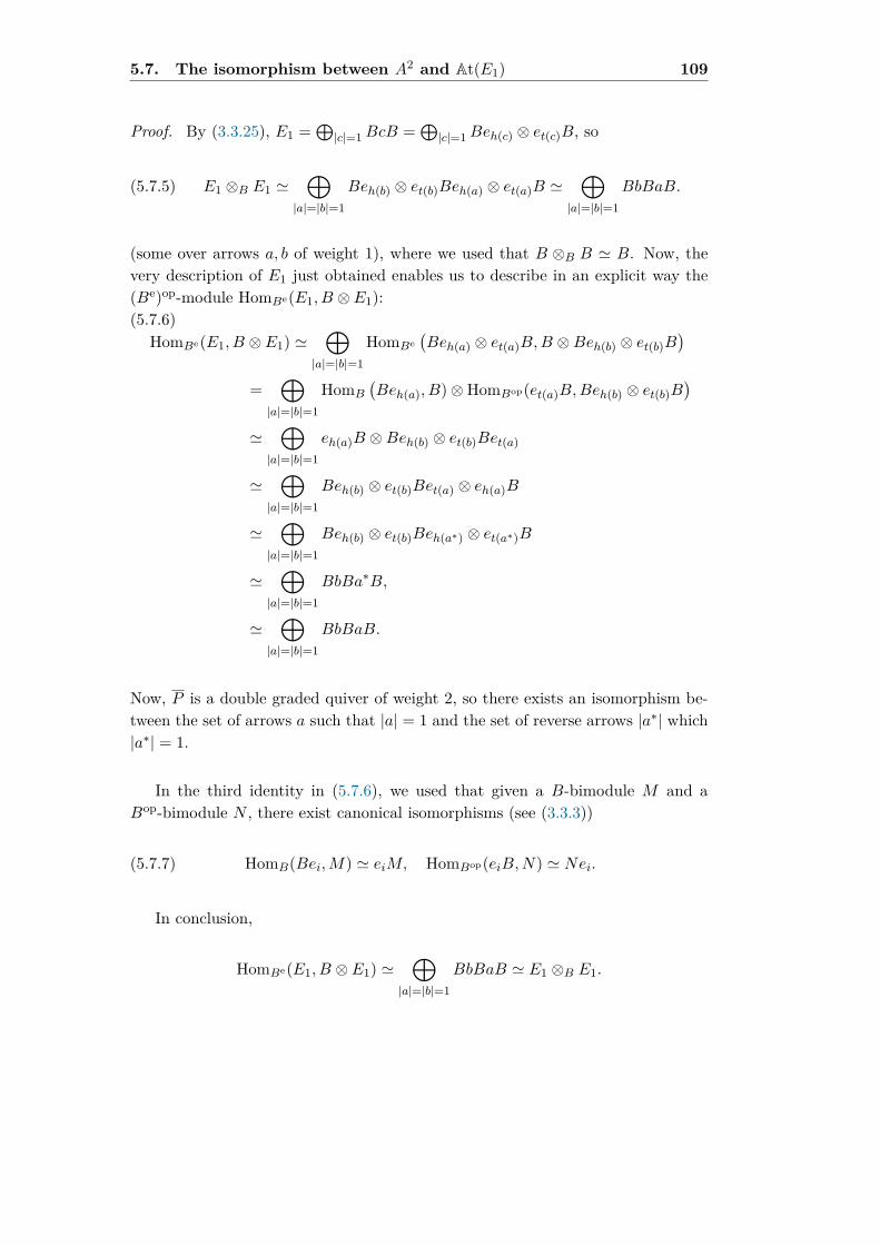
5.7. The isomorphism between A2 and At(E1) 109
Proof. By (3.3.25), E1 =⊕|c|=1BcB =
⊕|c|=1Beh(c) ⊗ et(c)B, so
(5.7.5) E1 ⊗B E1 '⊕
|a|=|b|=1
Beh(b) ⊗ et(b)Beh(a) ⊗ et(a)B '⊕
|a|=|b|=1
BbBaB.
(some over arrows a, b of weight 1), where we used that B ⊗B B ' B. Now, thevery description of E1 just obtained enables us to describe in an explicit way the(Be)op-module HomBe(E1, B ⊗ E1):(5.7.6)
HomBe(E1, B ⊗ E1) '⊕
|a|=|b|=1
HomBe(Beh(a) ⊗ et(a)B,B ⊗Beh(b) ⊗ et(b)B
)=
⊕|a|=|b|=1
HomB
(Beh(a), B)⊗HomBop(et(a)B,Beh(b) ⊗ et(b)B
)'
⊕|a|=|b|=1
eh(a)B ⊗Beh(b) ⊗ et(b)Bet(a)
'⊕
|a|=|b|=1
Beh(b) ⊗ et(b)Bet(a) ⊗ eh(a)B
'⊕
|a|=|b|=1
Beh(b) ⊗ et(b)Beh(a∗) ⊗ et(a∗)B
'⊕
|a|=|b|=1
BbBa∗B,
'⊕
|a|=|b|=1
BbBaB.
Now, P is a double graded quiver of weight 2, so there exists an isomorphism be-tween the set of arrows a such that |a| = 1 and the set of reverse arrows |a∗| which|a∗| = 1.
In the third identity in (5.7.6), we used that given a B-bimodule M and aBop-bimodule N , there exist canonical isomorphisms (see (3.3.3))
(5.7.7) HomB(Bei,M) ' eiM, HomBop(eiB,N) ' Nei.
In conclusion,
HomBe(E1, B ⊗ E1) '⊕
|a|=|b|=1
BbBaB ' E1 ⊗B E1.

110 Bi-symplectic tensor N-algebras of weight 2
In a similar way,(5.7.8)
HomBe(E1, E1 ⊗B) '⊕
|a|=|b|=1
HomBe(Beh(a) ⊗ et(a)B,Beh(b) ⊗ et(b)B ⊗B
)'
⊕|a|=|b|=1
HomB(Beh(a), Beh(b) ⊗ et(b)B)⊗HomBop(et(a)B,B)
'⊕
|a|=|b|=1
(eh(a)Beh(b) ⊗ et(b)B)⊗Bet(a)
'⊕
|a|=|b|=1
Bet(a) ⊗ eh(a)Beh(b) ⊗ et(b)B
'⊕
|a|=|b|=1
Ba∗BbB,
which also isomorphic to (5.7.5).
To describe a basis of adBe(E1), we shall now write explicitly the element inHomBe(BeE1,BE1⊗BB) which, under the isomorphisms in (5.7.8), corresponds tora∗qbp ∈
⊕|a|=|b|=1Ba
∗BbB, with r,q,p paths in B and the natural compatibilityconditions
eh(p) = et(b), eh(b) = et(q), eh(q) = eh(a), et(a) = et(r).
Here we used our convention that paths compose from right to left. The obtainedelement will be denoted [ra∗qbp]1 ∈ HomBe(BeE1,BE1⊗BB). If r′, q′, p′ are pathsin B, by a similar process, we determine [r′bq′a∗p′]2 ∈ HomBe(BeE1,BB ⊗ (E1)B)from r′bq′a∗p′ ∈
⊕|a|=|b|=1BbBa
∗B by means of (5.7.6). By (5.7.7) and thecanonical isomorphisms presented in §2.1.2, it is not difficult to see that:
(5.7.9)(E1 ⊗B E1)⊕ (E1 ⊗B E1)
∼=−→ EndBe(E1)(ra∗qbp, 0) 7−→ [ra∗qbp]1
(0, r′bq′a∗p′) 7−→ [r′bq′a∗p′]2,
where
[ra∗qbp]1 : E1 −→ BE1 ⊗BB : scs 7−→ δac(seh(a)qbp)⊗ (ret(a)s),
and
[r′bq′a∗p′]2 : E1 −→ BB ⊗ (E1)B : scs 7−→ δac(seh(a)p′)⊗ (r′bq′et(a)s).
Consequently, a basis of EndBe(E1) is given by [ra∗qbp]1 and [r′bq′a∗p′]2.
5.7.2 Description of a basis of adBe(E1)
To obtain a basis of adBe(E1), we impose the condition
(5.7.10) 〈a, f(b)〉L = −σ(132)〈b, f(a)〉L,
to a linear combination of our basis of EndBe(E1), where σ(123) : B ⊗ B ⊗ B →B ⊗B ⊗B : b1 ⊗ b2 ⊗ b3 7→ b2 ⊗ b3 ⊗ b1.
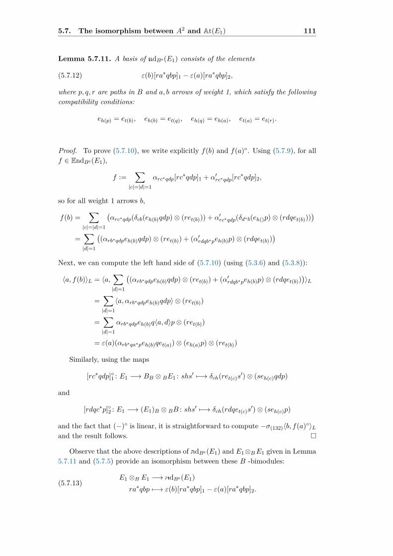
5.7. The isomorphism between A2 and At(E1) 111
Lemma 5.7.11. A basis of adBe(E1) consists of the elements
(5.7.12) ε(b)[ra∗qbp]1 − ε(a)[ra∗qbp]2,
where p, q, r are paths in B and a, b arrows of weight 1, which satisfy the followingcompatibility conditions:
eh(p) = et(b), eh(b) = et(q), eh(q) = eh(a), et(a) = et(r).
Proof. To prove (5.7.10), we write explicitly f(b) and f(a). Using (5.7.9), for allf ∈ EndBe(E1),
f :=∑
|c|=|d|=1
αrc∗qdp[rc∗qdp]1 + α′rc∗qdp[rc∗qdp]2,
so for all weight 1 arrows b,
f(b) =∑
|c|=|d|=1
(αrc∗qdp(δcb(eh(b)qdp)⊗ (ret(b))) + α′rc∗qdp(δd∗b(eh()p)⊗ (rdqet(b)))
)=∑|d|=1
((αrb∗qdpeh(b)qdp)⊗ (ret(b)) + (α′rdqb∗peh(b)p)⊗ (rdqet(b))
)Next, we can compute the left hand side of (5.7.10) (using (5.3.6) and (5.3.8)):
〈a, f(b)〉L = 〈a,∑|d|=1
((αrb∗qdpeh(b)qdp)⊗ (ret(b)) + (α′rdqb∗peh(b)p)⊗ (rdqet(b))
)〉L
=∑|d|=1
〈a, αrb∗qdpeh(b)qdp〉 ⊗ (ret(b))
=∑|d|=1
αrb∗qdpeh(b)q〈a, d〉p⊗ (ret(b))
= ε(a)(αrb∗qa∗peh(b)qet(a))⊗ (eh(a)p)⊗ (ret(b))
Similarly, using the maps
[rc∗qdp]1 : E1 −→ BB ⊗ BE1 : shs′ 7−→ δch(ret(c)s′)⊗ (seh(c)qdp)
and
[rdqc∗p]2 : E1 −→ (E1)B ⊗ BB : shs′ 7−→ δch(rdqet(c)s′)⊗ (seh(c)p)
and the fact that (−) is linear, it is straightforward to compute −σ(132)〈b, f(a)〉Land the result follows.
Observe that the above descriptions of adBe(E1) and E1⊗BE1 given in Lemma5.7.11 and (5.7.5) provide an isomorphism between these B -bimodules:
(5.7.13)E1 ⊗B E1 −→ adBe(E1)
ra∗qbp 7−→ ε(b)[ra∗qbp]1 − ε(a)[ra∗qbp]2.

112 Bi-symplectic tensor N-algebras of weight 2
5.7.3 The isomorphism Ψ|E1⊗BE1
In this subsection, we will compute the value of Ψ|E1⊗BE1 at basis elements ra∗qbpof E1 ⊗B E1:
Lemma 5.7.14. The map Ψ restricts to an isomorphism Ψ: E1 ⊗B E1∼=−→
adBe(E1), given byΨ(ra∗qbp) = [ra∗qbp]1 − [ra∗qbp]2,
where p, q, r are paths in B and a, b arrows of weight 1, which satisfy the followingcompatibility conditions:
eh(p) = et(b), eh(b) = et(q), eh(q) = eh(a), et(a) = et(r).
Proof. Firstly, note that since −,−ω is a double Poisson bracket of weight -2,Xra∗qbp(b′) = 0 for all b′ ∈ B, because by a simple application of the Leibniz ruleand (5.3.2):
Xra∗qbp(b′) = −σ(12)(ra∗
b′, qbp
ω
+b′, ra∗
ωqbp)
= 0.
Thus,
(5.7.15) Ψ|E1⊗BE1 : E1 ⊗B E1 −→ adBe(E1).
We apply the (graded) Leibniz rule when c is an arrow of weight 1:
(5.7.16)Dra∗qbp(c) = ra∗qbp, cω
= −σ(12) c, ra∗qbpω= −σ(12) (ra∗q c, bω p+ r c, a∗ω qbp) .
To compute c, bω and c, a∗ω we shall use Proposition 2.3.18 and, as aconsequence, to address the question of the description of the differential doublePoisson bracket P in the setting of quivers (recall Definition 2.3.21). M. Van denBergh shows in [96] §6.2, that the double Schouten–Nijenhuis bracket acquires avery simple form in this case:
Proposition 5.7.17 ([96], Proposition 6.2.1). Let A = kQ and a, b ∈ Q. Then
a, b = 0∂
∂a, b
=eh(a) ⊗ et(a) if a = b
0 otherwise∂
∂a,∂
∂b
= 0
Note that in our convention, arrows compose from to left. The followingresult provides an explicit description of the differential double Poisson bracketP ∈ (TADerB A)2 (see §2.3.3) in the context of double graded quivers:

5.7. The isomorphism between A2 and At(E1) 113
Proposition 5.7.18 ([96], Theorem 6.3.1). Let A = kP be the graded path algebraof the double graded quiver P . Then A has the following differential double Poissonbracket
(5.7.19) P =∑a∈P
∂
∂aε(a) ∂
∂a∗.
Applying now Propositions 2.3.18, 5.7.18 and 5.7.17 we can calculate
(5.7.20)
c, bω = −c, P, bL
=c,m
(ε(b)(eh(b) ⊗ et(b)) ∗
∂
∂b∗
)L
= σ(12)
ε(b) ∂
∂b∗, c
= ε(b)eh(b) ⊗ et(b),
where m : A⊗ A→ A⊗ A : a⊗ b 7→ ab is the multiplication. Replacing b by a∗ in(5.7.20), we obtain
(5.7.21) c, a∗ω = −ε(a)et(a) ⊗ eh(a).
Using now (5.7.20) and (5.7.21) in (5.7.16), we can conclude
Dra∗qbp(c) = −σ(12) (ra∗q c, bω p+ r c, a∗ω qbp)= ε(b)eh(a)qbp⊗ ret(a) − ε(a)eh(a)p⊗ rbqet(a)
SoΨ|E1⊗BE1(ra∗qbp) = ε(b)[ra∗qbp]1 − ε(a)[ra∗qbp]2.


Chapter 6
Non-commutative Courant algebroids
In Chapter 6, we calculate the non-commutative structures that arise when weequip a graded bi-symplectic tensor algebra (A,ω) of weight 2 with a homologicaldouble derivation Q. Here, a double derivation Q on A is homological if it satisfiesthe “double Maurer–Cartan” equation Q,Q = 0, where −,− is the doubleSchouten–Nijenhuis commutator. Since our calculations will be based on results ofChapter 4, we focus on the case where (A,ω) is a bi-symplectic graded path algebraof a double graded quiver (see (3.3.4)). The new algebraic structures will be called“double Courant–Dorfman algebras”. They are non-commutative versions of theCourant–Dorfman algebras introduced by Roytenberg [83], that themselves are toCourant algebroids what Lie–Rinehart algebras are to Lie algebroids.
In §6.1, we start with a short review of the role of Courant algebroids ingeometry and physics (§6.1.1) and their definition §6.1.2. In §6.2 we provide analgebraic reformulation of Roytenberg’s correspondence between symplectic NQ-manifolds of weight 2 and Courant algebroids. Finally, in §6.3.1 we define thecentral object of this chapter –double Courant–Dorfman algebras–, and show thata bi-symplectic NQ-algebra (A,ω) attached to a double graded quiver P determinesa double Courant–Dorfman algebra over the path algebra of the weight 0 subquiverQ of P .
6.1 Courant algebroids
6.1.1 A brief historical account of Courant algebroids
Following [62], the origins of Courant algebroids can be found in the article [25]written by A. Weinstein and T. Courant who interpreted Dirac’s bracket appearedin [32] in a geometric way by constructing a framework where Poisson and pre-symplectic structures were unified. Two years later, in his thesis [26], Courantdefined a skew-symmetric bracket on TM ⊕ T∗M (called the Courant bracket)which, in general, is not a Lie-algebra bracket because the Jacobi identity does not
115

116 Non-commutative Courant algebroids
hold. For sections X + ξ and Y + η of TM ⊕ T∗M , this bracket is
[[ X + ξ, Y + η ]] = [X,Y ] + LXη − LY ξ −12 d(iXη − iY ξ).
Note that Dirac structures of Courant and Weinstein coincide with those of IreneYa. Dorfman as defined in 1987 in her article [34].
In [70], Liu, Weinstein and Xu systematized the properties of the bracket intro-duced by Courant in the definition of Courant algebroid. This structure on a vectorbundle E →M involves an antisymmetric bracket on the sections of E whose “Ja-cobi anomaly” has an explicit expression in terms of a bundle map E → TM and afield of symmetric bilinear forms on E. In [80], D. Roytenberg twisted the bracketin a Courant algebroid by adding a symmetric term (already suggested in [70]). Asa consequence, he sacrificed skew-symmetry, but he obtained an equivalent (andmore natural) definition of a Courant algebroid because the Jacobi identity in thisnon skew-symmetric setting resembles a Leibniz rule.
Roytenberg plays a central role in this history since he had the insight of seeingCourant algebroids as graded objects. In [81], he proved that symplectic NQ-manifolds of weight 2 are in one-to-one correspondence with Courant algebroids;this theorem will be explained in §6.2. Later, he defined algebraic relatives ofCourant algebroids: Courant–Dorfman algebras [83].
N. Hitchin and M. Gualtieri developed Generalized complex geometry (see [49]and [45]) which can be regarded as a way of unifying complex and symplectic geom-etry by taking the idea that both structures should be thought as linear operationson T⊕T∗.
Finally, Courant algebroids have turned out to be interesting objects in Physics.In [82] it was showed that the AKSZ procedure yields a canonical three-dimensionalTopological Field Theory associated to any Courant algebroid. Moreover, in [88](see also [89]), Ševera presented Courant algebroids as the natural framework todeal with two-dimensional variational problems and, as a consequence, they seemthe natural framework of string theory.
6.1.2 Definition of Courant algebroids
From now on, k is a field of characteristic zero, R is a commutative algebra and Bis a smooth commutative R-algebra.
As in §5.1, (A,ω) is a symplectic polynomial N-algebra of weight 2 such thatA = SymB(E1[−1] ⊕ E2[−2]), where E1 and E2 are projective finitely generatedB-modules, and SymB(−) denotes the graded symmetric algebra over B. Then,by Lemma 4.1.12, this structure induces a Poisson bracket of weight -2 (which

6.1. Courant algebroids 117
is denoted −,−ω) and it is completely determined by the projective finitelygenerated B-module E1 equipped with a symmetric non-degenerate bilinear form(the inner product) 〈−,−〉 : E1 × E1 → B (see §5.1.6). In order to simplify ourexposition, we make the identification E := E1.
Definition 6.1.1. A pre-Courant algebroid over B is a 4-tuple(E, 〈−,−〉, ρ, [[ −,− ]] ) consisting of is a projective finitely generated B-moduleE endowed with a symmetric non-degenerate bilinear form (the inner product),
〈−,−〉 : E × E −→ B,
a B-module morphism ρ : E → DerRB, called the anchor, and a R-bilinearoperation
[[ −,− ]] : E × E −→ E,
called the Dorfman bracket. These data must satisfy the following conditions:
[[ e1, be2 ]] = ρ(e1)(b)e2 + b [[ e1, e2 ]] ,(6.1.2a)
[[ e1, e1 ]] = 12ρ∗ d(〈(e1, e1)〉,(6.1.2b)
ρ(e1)(〈e2, e2〉) = 2〈 [[ e1, e2 ]] , e2〉,(6.1.2c)
for all b ∈ B and e1, e2 ∈ E. Moreover, if the bracket satisfies the Jacobi identity
(6.1.3) [[ e1, [[ e2, e3 ]] ]] = [[ [[ e1, e2 ]] , e3 ]] + [[ e2, [[ e1, e3 ]] ]] ,
for all e1, e2, e3 ∈ E, then (E, g, ρ, [[ −,− ]] ) is called a Courant algebroid over B.
In (6.1.2b), d is the de Rham differential, E ' E∗ via 〈−,−〉 and ρ∗ : Ω1RA →
E∗ ' E is the dual map of ρ. In other words, 〈e, ρ∗ db〉 = ρ(e)(f) for all b ∈ B ande ∈ E.
Remark 6.1.4. Observe that Definition 6.1.1 is an algebraic adaptation of [44],§5.1. We point out that this definition is equivalent to [83], Definition 2.1. Royten-berg defines a Courant–Dorfman algebra as a 5-tuple (R, E , 〈−,−〉, ∂, [−,−]). Thedifference with respect to Definition 6.1.1 is the derivation ∂ : B → E is a deriva-tion, but, by (6.1.2a), ρ(e)b = 〈e, ∂b〉 and it follows the equivalence of both defini-tions.
Remark 6.1.5. Following [81] (and [80]), in this thesis we shall use the notionof Courant algebroid which satisfies the Jacobi identity (6.1.3) but it is not skew-symmetric. By (6.1.2b), it is not difficult to see that the Dorfman bracket satisfiesthe following identity:
[[ e1, e2 ]] = − [[ e2, e1 ]] + ρ∗ dg(e1, e2)
Note that there exists an equivalent notion of Courant algebroid, in which theoperation (called the Courant bracket) is skew-symmetric but it satisfies the Jacobiidentity only up to an exact term (given in terms of the derivative of the Jacobiator)(see [45], §3.2 and [80], Definition 2.3.2).

118 Non-commutative Courant algebroids
6.1.3 Connections and torsion on Courant algebroids
Let E be a Courant algebroid over B, ρ its anchor and F another finitely generatedprojective B-module.
Definition 6.1.6 (E-connection, [3]). A linear map ∇ : E ⊗ F → F is called anE-connection on F if it satisfies the following properties,
∇bef = b∇ef,(6.1.7a)∇e(bf) = b∇ef + ρ(e)(b)f,(6.1.7b)
where e ∈ E, f ∈ F and b ∈ B.
Note that given an ordinary connection ∇ over F , we can define an E-connection using ∇es := ∇ρ(e)s.
One can find at least three definitions of torsion of an E-connection ([3] and[44], [46] and [54]). In this thesis, we will use a variant of [54], with a slight changein the sign conventions.
Definition 6.1.8 (E-torsion). Let (E, g, ρ, [[ −,− ]] ) be a Courant algebroid overB with a connection ∇. Then the weight 3 map C∇ : (E∗)⊗3 → B defined by
(6.1.9) 〈C∇, e1 ⊗ e2 ⊗ e3〉 = 〈 [[ e1, e2 ]]−∇ρ(e1)e2 +∇ρ(e2)e1, e3〉+ 〈∇ρ(e3)e1, e2〉,
will be called the E-torsion.
Observe that this map is linear in e3.
6.2 Courant algebroids and symplectic NQ-algebras ofweight 2
Yvette Kosmann-Schwarzbach introduced the notion of derived bracket in [61]showing that the Dorfman bracket on T⊕T∗ is a derived bracket of the commutatorof endomorphisms of the space of differential forms by the de Rham differential.Moreover, Vaintrob in [94] interpreted Lie algebroids as an odd-self-commutingvector field on a supermanifold. In [81], Roytenberg proved the equivalence betweenCourant algebroids and symplectic NQ-algebras of weight 2, which will be explainedin this section. The idea is that the structure of a Courant algebroid is encodedby an element S ∈ A3 such that S, Sω = 0. Observe that, in some sense, Sgeneralizes the Cartan 3-form on a quadratic Lie algebra appearing in the Chern–Simons theory (see [82]).
6.2.1 Bijection between pre-Courant algebroids and weight 3functions
Recall (see §4.1) that an NQ-manifold (M, Q) is an N-manifold endowed with anintegrable homological vector field Q of weight +1 (i.e. [Q,Q] = 2Q2 = 0, where

6.2. Courant algebroids and symplectic NQ-algebras of weight 2 119
[−,−] denotes the Schouten bracket of multi-derivations). In addition, a symplecticNQ-manifold (M, ω,Q) is an NQ-manifold whose homological vector field is com-patible with ω in the sense that LQω = 0, where LQ stands for the Lie derivativealong the vector field Q.
Let R be a commutative k-algebra, where k is a field of characteristic zero andB a smooth commutative R-algebra. Following §4.1.3 (and [20]), if (A,ω,Q) is asymplectic NQ-algebra over B of weight 2 (see Definition 4.1.15) with A0 = B, weshall show that the relation [Q,Q] = 0 is equivalent to S, Sω = 0, where S ∈ A3
and −,−ω is the Poisson bracket of weight -2 induced by ω via (4.1.7).
Since Q is a symplectic homological derivation, it satisfies LQω = 0 and[Q,Q] = 0, by Lemma 4.1.6(ii), we have
Q = HS = S,−ω,
where S ∈ A. In fact, by definition, Q has weight +1 and the identity for all b ∈ BS, bω = HS(b) = Q(b) yields
|S| = |Q| − |−,−ω| = 3.
Thus S ∈ A3. Now, by the Jacobi identity we have the identity Ha,bω = [Ha, Hb]which applied to a = b = S gives
HS,Sω = [Q,Q].
Therefore, if a ∈ A,
[Q,Q](a) = HS,Sω(a) = S, Sω, aω,
and the relation [Q,Q] = 0 is equivalent to S, Sω ∈ B because the equation(4.1.4) provides S, Sω ∈ R but B is a commutative R-algebra. However, S, Sωhas weight 4 because |S| = 3. Therefore, we conclude that S, Sω = 0 as weclaimed.
The following result is important because states that the function S ∈ A3
obtained in the previous discussion encodes the structure of pre-Courant algebroidintroduced in Definition 6.1.1:
Proposition 6.2.1. Every weight 3 function S ∈ A3 induces a pre-Courantalgebroid structure on (E, g) by setting
ρ(e1)(b) := S, e1ω, bω,(6.2.2a)[[ e1, e2 ]] := S, e1ω, e2ω,(6.2.2b)
for all b ∈ B and e1, e2 ∈ E. Conversely, given a pre-Courant algebroid, we canconstruct the weight 3 function S = ρ+ C∇ which satisfies (6.2.2).

120 Non-commutative Courant algebroids
Proof. The Poisson bracket of weight -2 −,−ω induced by the symplectic formω will be denoted by −,− whereas the inner product 〈−,−〉 by g(−,−). ByDefinition 6.1.1, we have to check (6.1.2a) - (6.1.2c). Using the fact that −,− isa derivation in its second argument,
[[ e1, be2 ]] = bS, e1, e2+ S, e1, be2
= b [[ e1, e2 ]] + ρ(e1)(b)e2.
To prove (6.1.2b), since −,− is a bracket of weight -2, e1, e2, e2 = 0 whene1, e2 ∈ E. Then, applying the Jacobi identity (4.1.11):
0 = S, e1, e2, e2= S, e1, e2, e2 − e1, S, e2, e2= S, e1, e2, e2 − e1, S, e2, e2 − e2, S, e2= S, e1, e2, e2 − 2e1, S, e2, e2,
where we used that e2, S, e2 = −S, e2, e2. Hence, since ξ, η = g(ξ, η),when ξ, η ∈ A1, we obtain identity
ρ(e1)(g(e2, e2)) = 2g(e1, [[ e2, e2 ]] ).
Finally, as ρ(e1)(g(e2, e2)) = g(e1, ρ∗ dg(e2, e2)) and g is a non-degenerate bilinear
form by hypothesis, we get (6.1.2b). The proof of (6.1.2c) is a simple applicationof the Jacobi identity:
ρ(e1)(g(e2, e2)) = S, e1, e2, e2= S, e1, e2, e2+ e2, S, e1, e2= g( [[ e1, e2 ]] , e2) + g( [[ e1, e2 ]] , e2)= 2g( [[ e1, e2 ]] , e2),
where, again, we used that e1, e2 := g(e1, e2) for e1, e2 ∈ E.
Conversely, given a pre-Courant algebroid, we construct the weight 3 functionS = ρ + C∇ and we shall prove that it satisfies (6.2.2). This proof was kindlycommunicated to the author by Jean-Philippe Michel.
First observe that both the torsion map and the anchor map ρ are weight 3functions; ρ can be identified with an element of E⊗DerRB using the inner prod-uct g (recall that E2 ' DerRB). Thus, S = ρ+ C∇ is a weight 3 function on A.
Next, it is easy to see that S satisfies (6.2.2a). To prove that S satisfies (6.2.2b),using sheaf theory, recall that a parallel section e ∈ E satisfies ∇Xe = 0 for allX ∈ DerRB. Furthermore, a general section is a finite linear combination of termsof the form be, where b ∈ B and e ∈ E is a parallel section. Now, we shall writethe structure of the proof:
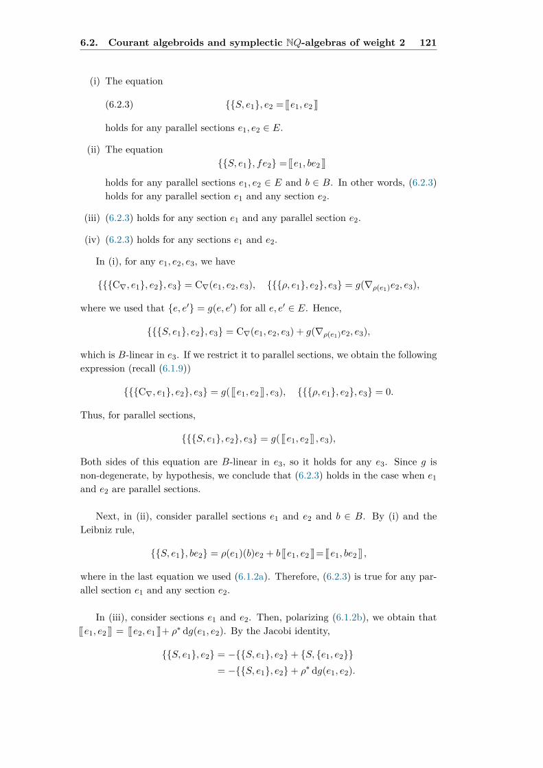
6.2. Courant algebroids and symplectic NQ-algebras of weight 2 121
(i) The equation
(6.2.3) S, e1, e2 = [[ e1, e2 ]]
holds for any parallel sections e1, e2 ∈ E.
(ii) The equationS, e1, fe2 = [[ e1, be2 ]]
holds for any parallel sections e1, e2 ∈ E and b ∈ B. In other words, (6.2.3)holds for any parallel section e1 and any section e2.
(iii) (6.2.3) holds for any section e1 and any parallel section e2.
(iv) (6.2.3) holds for any sections e1 and e2.
In (i), for any e1, e2, e3, we have
C∇, e1, e2, e3 = C∇(e1, e2, e3), ρ, e1, e2, e3 = g(∇ρ(e1)e2, e3),
where we used that e, e′ = g(e, e′) for all e, e′ ∈ E. Hence,
S, e1, e2, e3 = C∇(e1, e2, e3) + g(∇ρ(e1)e2, e3),
which is B-linear in e3. If we restrict it to parallel sections, we obtain the followingexpression (recall (6.1.9))
C∇, e1, e2, e3 = g( [[ e1, e2 ]] , e3), ρ, e1, e2, e3 = 0.
Thus, for parallel sections,
S, e1, e2, e3 = g( [[ e1, e2 ]] , e3),
Both sides of this equation are B-linear in e3, so it holds for any e3. Since g isnon-degenerate, by hypothesis, we conclude that (6.2.3) holds in the case when e1and e2 are parallel sections.
Next, in (ii), consider parallel sections e1 and e2 and b ∈ B. By (i) and theLeibniz rule,
S, e1, be2 = ρ(e1)(b)e2 + b [[ e1, e2 ]] = [[ e1, be2 ]] ,
where in the last equation we used (6.1.2a). Therefore, (6.2.3) is true for any par-allel section e1 and any section e2.
In (iii), consider sections e1 and e2. Then, polarizing (6.1.2b), we obtain that[[ e1, e2 ]] = [[ e2, e1 ]] + ρ∗ dg(e1, e2). By the Jacobi identity,
S, e1, e2 = −S, e1, e2+ S, e1, e2= −S, e1, e2+ ρ∗ dg(e1, e2).

122 Non-commutative Courant algebroids
So, if (6.2.3) holds for [[ e1, e2 ]] , then it holds also for [[ e2, e1 ]] . Together with (ii),this implies that (6.2.3) holds for any section e1, and any parallel section e2.
Finally, in the last item, consider parallel sections e1 and e2 and b, b′ ∈ B.Then, applying (6.1.2a),
[[ be1, b′e2 ]] = b′ [[ be1, e2 ]] + ρ(be1)(b′)e2
= b′S, be1, e2+ S, be1, b′e2
= S, be1, b′e2,
where in the second equation we applied (iii) and (6.2.2a), whereas in the last one,we used the Leibniz rule for −,−. So, we can conclude that (6.2.3) holds for anysections e1 and e2.
6.2.2 Courant algebroids and the homological condition
Proposition 6.2.4. The Jacobi identity (6.1.3) for [[ −,− ]] is equivalent to thehomological condition S, Sω = 0.
Proof. The Poisson bracket of weight -2 −,−ω induced by the symplectic formω will be denoted by −,− whereas the inner product 〈−,−〉 by g(−,−). Weshall prove the following Jacobi identity
(6.2.5) [[ e1, [[ e2, e3 ]] ]] = [[ [[ e1, e2 ]] , e3 ]] + [[ e2, [[ e1, e3 ]] ]] .
(6.2.2b) provides
[[ e1, [[ e2, e3 ]] ]] = S, e1, [[ e2, e3 ]] = S, e1, S, e2, e3= S, e1, S, e2, e3+ S, e2, S, e1, e3,
where we applied the Jacobi identity (4.1.11) for −,−. By the same reason andusing that S, S = 0,
S, S, e1, e2 = S, S, e1, e2+ S, e1, S, e2
= 12S, S, e1+ S, e1, S, e2
= S, e1, S, e2,
Then,
[[ e1, [[ e2, e3 ]] ]] = S, S, e1, e2+ S, e2, S, e1, e3= [[ [[ e1, e2 ]] , e3 ]] + [[ e2, [[ e1, e3 ]] ]] .
Conversely, following [54], it is not difficult to see that as a consequence of theJacobi identity for [[ −,− ]] ,we obtain the expression for all e1, e2, e3 ∈ E.
(6.2.6) S, S, e1, e2, e3 = 0

6.3. Non-commutative Courant algebroids 123
Now, let b ∈ B. Then, by the Leibniz rule for −,− in the second argument,
0 = S, S, e1, e2, be3= bS, S, e1, e2, e3+ S, S, e1, e2, be3.
By (6.2.6), we obtain
(6.2.7) S, S, e1, e2, b = 0
Finally, by another application of the Jacobi identity and (6.2.7), for alle1, e2 ∈ E and b ∈ B,
0 = S, S, e1, e2, b= S, S, e2, e1, b+ S, S, e1, e2, b= S, S, e1, e2, b
The key point now is that every b′ ∈ B can be written b′ = e1, e2 withappropriate e1, e2 ∈ E. Therefore, we conclude that
S, S, b′, b = 0,
for all b, b′ ∈ B, which implies that S, S = 0, as required.
6.3 Non-commutative Courant algebroids
6.3.1 Definition of double Courant–Dorfman algebras
Following Definition 6.1.1, in this section we introduce the notion of a doubleCourant–Dorfman algebras.
Let k be a field of characteristic zero, R be a finite dimensional semisimpleassociative k-algebra and B an associative R-algebra. Recall that in Chapter 3 andChapter 5, we proved that the structure of a given bi-symplectic tensor N-algebra(A,ω) of weight 2 corresponds to a pair (E1, 〈−,−〉), where E1 is a projectivefinitely generated B-bimodule and 〈−,−〉 is the symmetric non-degenerate pairingdefined in (5.3.6) (see Theorem 5.7.1). To simplify our exposition, we make theidentification E := E1 and, if necessary, 〈−,−〉 := 〈−,−〉L, which was defined in(5.3.8).
Definition 6.3.1 (Double Courant–Dorfman algebra). A double pre-Courant–Dorfman algebra over B is a 4-tuple (E, 〈−,−〉, ρ, [[ −,− ]] ) consisting of a projectivefinitely generated B-bimodule E endowed with a symmetric non-degenerate pairing(the inner product)
〈−,−〉 : E ⊗ E −→ B ⊗B,
a B-bimodule morphism
(6.3.2) ρ : E −→ DerRB,

124 Non-commutative Courant algebroids
called the anchor, and an operation
(6.3.3) [[ −,− ]] : E ⊗ E −→ (E ⊗B)⊕ (B ⊗ E),
called the double Dorfman bracket, which is R-linear for the outer bimodulestructure on B ⊗ B in the second argument and R-linear for the inner bimodulestructure on B ⊗ B in the first argument. These data must satisfy the followingconditions:
[[ e1, be2 ]] = ρ(e1)(b)e2 + b [[ e1, e2 ]] ,(6.3.4a)[[ e1, e2b ]] = e2ρ(e1)(b) + [[ e1, e2 ]] b,(6.3.4b)
[[ be1, e2 ]] = e1 ∗ σ(12)ρ(e2)(b)e1 + b ∗ [[ e1, e2 ]] ,(6.3.4c)[[ e1b, e2 ]] = e1 ∗ σ(12)ρ(e2)(b) + [[ e1, e2 ]] ∗ b,(6.3.4d)
ρ∨ d〈e1, e1〉 = [[ e1, e1 ]] + [[ e1, e1 ]] ,(6.3.4e)ρ(e1)(〈e2, e2〉) = τ(132)〈e2, [[ e1, e2 ]] 〉+ τ(123)〈e2, [[ e1, e2 ]] 〉,(6.3.4f)
for all b ∈ B and e1, e2 ∈ E. If the bracket [[ −,− ]] satisfies the double Jacobiidentity:
(6.3.5) τ(123) [[ e1, [[ e2, e3 ]] ]] L + τ(123) [[ e2, [[ e1, e3 ]] ]] L + [[ [[ e1, e2 ]] , e3 ]] L = 0
for all e1, e2, e3 ∈ E, then (E, 〈−,−〉, ρ, [[ −,− ]] ) is called a double Courant–Dorfmanalgebra.
In (6.3.4c) and (6.3.4d), σ(12) denotes the permutation A ⊗ A → A ⊗ A :a1⊗a2 7→ a2⊗a1, whereas in (6.3.4e) d : A→ Ω1
RA is the de Rham differential, andρ∨ : Ω1
RA → E∨ ' E is the composite of the canonical map Ω1RB → (DerRB)∨,
HomBe(ρ,BeBe) : (DerRB)∨ → E∨, and the isomorphism E∨ ' E induced by〈−,−〉 (see (5.3.5)). By convention, in (6.3.4e),
ρ∨ d〈e1, e1〉 = ρ∨ d(〈e1, e1〉′ ⊗ 〈e1, e1〉′′)= ρ∨(d(〈e1, e1〉′)⊗ 〈e1, e1〉′′ + 〈e1, e1〉′ ⊗ ρ∨(d(〈e1, e1〉′′)).
Similarly, we use this convention for ρ(e1)(〈e2, e2〉) in (6.3.4f). As in thecommutative case, we will use of the identification
〈e, ρ∨ db〉 = ρ(e)(b)
for all e ∈ E and b ∈ B.
It will be useful to define 〈−,−〉 : E⊗B⊕B⊗E → B⊗B⊗B by the formulae(see (5.3.8))
〈e⊗ b, e′〉 = 0, 〈b⊗ e, e′〉 = b⊗ 〈e, e′〉.
It will also be useful to apply Sweedler’s notation to the double Dorfman bracket:
[[ −,− ]] = [[ −,− ]] l + [[ −,− ]] r,

6.4. Double Courant algebroids and bi-symplectic NQ-algebras ofweight 2 125
where
[[ −,− ]] l = [[ −,− ]] ′l ⊗ [[ −,− ]] ′′l : E ⊗ E −→ E ⊗B,[[ −,− ]] r = [[ −,− ]] ′r ⊗ [[ −,− ]] ′′r : E ⊗ E −→ B ⊗ E,
Then, for i = l, r,[[ e, e′ ]] i = − [[ e′, e ]] ′′i ⊗ [[ e′, e ]] ′i
and so the brackets appearing in the double Jacobi identity (6.3.5) are sums ofterms of the following types
[[ e, [[ e′, e′′ ]] ′i ⊗ [[ e′, e′′ ]] ′′i ]] L = [[ e, [[ e′, e′′ ]] ′i ]]⊗ [[ e′, e′′ ]] ′′i ,[[ [[ e′, e′′ ]] ′i ⊗ [[ e′, e′′ ]] ′′i , e ]] L = [[ [[ e′, e′′ ]] ′i, e ]]⊗ [[ e′, e′′ ]] ′′i ,[[ e, [[ e′, e′′ ]] ′i ⊗ [[ e′, e′′ ]] ′′i ]] L = [[ e, [[ e′, e′′ ]] ′i ]] ⊗ [[ e′, e′′ ]] ′′i ,[[ [[ e′, e′′ ]] ′i ⊗ [[ e′, e′′ ]] ′′i , e ]] L = [[ [[ e′, e′′ ]] ′i, e ]] ⊗ [[ e′, e′′ ]] ′′i ,
for all e, e′, e′′ ∈ E.
6.4 Double Courant algebroids and bi-symplectic NQ-algebras of weight 2
The main goal of this section is to explore the connection between bi-symplecticNQ-algebras of weight 2 (see Definition 4.3.1) and double Courant–Dorfman alge-bras. As in the commutative case, by Lemma 2.5.6, a bi-symplectic double deriva-tion is a Hamiltonian double derivation. Thus, we can write Q = S,−ω, where−,−ω is the double Poisson bracket of weight -2 induced by ω and S ∈ A3.The idea is that we should expect such a S encodes the structure of a doublepre-Courant–Dorfman algebra, recoverable via derived brackets and, if in addition,S, Sω = 0 (here −,−ω denotes the associated bracket to −,−ω), then weshall obtain the structure of a double Courant–Dorfman algebra.
From now on, we fix the following framework: let R be a finite dimensionalsemisimple associative k-algebra, where k is a field of characteristic zero, and B
a smooth associative R-algebra. Let (A,ω,Q) be a bi-symplectic NQ-algebra ofweight 2 over R such that A0 = B. In particular, let Q be a bi-symplectic ho-mological double derivation, that is, |Q| = +1, LQω = 0 and Q,Q = 0, where−,− is the graded double Schouten–Nijenhuis bracket on TADerRA. First, weshow that the identity Q,Q = 0 is equivalent to S, Sω = 0.
By Lemma 2.5.6(ii), ιQω = dS for some θ ∈ A, that is,
(6.4.1) Q = S,−ω
where S ∈ A. Now, for all a ∈ A, the identity S, aω = Q(a) implies
|S| = |Q| − |−,−ω| = 3,

126 Non-commutative Courant algebroids
that is, S ∈ A3. Now, the identity Ha,bω = Ha, Hb (see Proposition 2.4.6)applied to a = b = S gives
HS,Sω = Q,Q .
Therefore the relation Q,Q = 0 is equivalent to S, Sω ∈ B ⊗ B because, by(2.4.2), HS,Sω = 0 implies that 0 = dS, Sω = dS, S′ω⊗S, S
′′ω+S, S′ω⊗
dS, S′′ω, which implies that S, S′ω , S, S′′ω ∈ R. Finally, since B is an asso-
ciative R-algebra, we conclude that S, S′ω , S, S′′ω ∈ B as we required and, as
a consequence, |S, Sω| = 0. However, S, Sω has weight 4 because |S| = 3. SoS, Sω = 0.
Next, as we wrote above, we shall prove that the structure of double pre-Courant algebroid can be recovered by means of derived brackets as the followingresult shows:
Proposition 6.4.2. Every weight 3 function S ∈ A3 induces a double pre-Courant–Dorfman algebra structure on (E, 〈−,−〉) by setting
ρ(e1)(b) := S, e1ω, bω ,(6.4.3a)[[ e1, e2 ]] := S, e1ω, e2ω ,(6.4.3b)
for all b ∈ B and e1, e2 ∈ E, and where −,− = m −,−ω is the associatedbracket in A (see (2.3.5)).
Remark 6.4.4. In this section, we will use the associated bracket. Then we havea graded version of (2.3.8) (cf. [2])
(6.4.5) a, b, c = a, b, c+ (−1)|a||b|b, a, c.
Finally, recall that a,− acts on tensors by a, u⊗ v := a, u ⊗ v + u⊗ a, v.
Proof. For sake of simplicity, the double Poisson bracket of weight -2 −,−ωinduced by the bi-symplectic form ω will be denoted by −,− and the non-degenerate symmetric pairing 〈−,−〉 by g(−,−). In order to prove (6.3.4a) inDefinition 6.3.1, we shall use the fact that −,− is a double derivation in itssecond argument with respect to the outer bimodule structure:
[[ e1, be2 ]] = S, e1, be2= b S, e1, e2+ S, e1, b e2
= b [[ e1, e2 ]] + ρ(e1)(b)e2
The proof that [[ e1, e2b ]] = e2ρ(e1)(b) + [[ e1, e2 ]] b holds is quite similar. (6.3.4c) and(6.3.4d) also follow easily. To prove (6.3.4e), note that since −,− is a doublePoisson bracket of weight -2, e1, e2, e2L = 0. Then, by (2.3.7):
0 = S, e1, e2, e2L= S, e1, e2, e2L − e1, S, e2, e2L= S, e1, e2, e2L − e1, S, e2, e2 − e2, S, e2L= S, e1, e2, e2L − e1, S, e2, e2+ S, e2, e2L

6.4. Double Courant algebroids and bi-symplectic NQ-algebras ofweight 2 127
By definition, if e, e′ ∈ E, e, e′ = g(e, e′), so
ρ(e1)(g(e2, e2)) = g(e1, [[ e2, e2 ]] + [[ e2, e2 ]] )
Next, since g is non-degenerate, the identity
g(e1, ρ∨ dg(e2, e2)) = g(e1, [[ e2, e2 ]] + [[ e2, e2 ]] )
implies (6.3.4c). Finally, the key ingredient to prove (6.3.4d) holds is the doubleJacobi identity for −,− (see (2.3.12)):
−ρ(e1)(g(e2, e2)) = −S, e1, g(e2, e2)L= τ(123) e2, e2, S, e1L − τ(132) e2, S, e1, e2L= −τ(123) e2, [[ e1, e2 ]] L − τ(132) e2, [[ e1, e2 ]] L= −τ(123) g(e2, [[ e1, e2 ]] )− τ(132) g(e2, [[ e1, e2 ]] )
Finally, at the beginning of this subsection, we showed that the fact that thehomological double derivation Q satisfied Q,Q = 0 implied S, Sω = 0. Inthe next result, we prove that the weaker condition S, Sω = 0 (where −,−ω isthe associated bracket) implies the double Jacobi identity (6.3.5).
Proposition 6.4.6. If S, Sω = 0 then the double Jacobi identity in (6.3.5) holds.
Proof. As usual, −,−ω to be denoted −,−ω. By (6.4.3b),
[[ e1, [[ e2, e3 ]] ]] L = S, e1, S, e2, e3Land applying the double Jacobi identity (2.3.12),
(6.4.7)−τ(123)[[ e1, [[ e2, e3 ]] ]] L = τ(132) S, e2, e3, S, e1L +
+ e3, S, e1, S, e2LNext, we shall focus on e3, S, e1, S, e2L and use (2.3.7):
S, S, e1, e2 = S, S, e1, e2+ S, e1, S, e2
Since (A, −,−) is a Loday algebra, by (6.4.5),
S, S, e1 = S, S, e1 − S, S, e1
Thus, since S, S = 0 by hypothesis, we obtain the following identity:
e3, S, e1, S, e2L = e3, S, S, e1, e2LHence, we make the substitution in (6.4.7):
−τ(123)[[ e1, [[ e2, e3 ]] ]] L = τ(132) S, e2, e3, S, e1L+ e3, S, S, e1, e2L= τ(132) S, e2, S, e1, e3L ++ S, S, e1, e2, e3L= τ(132) S, e2, [[ e1, e3 ]] L + S, S, [[ e1, e2 ]], e3L= τ(132) [[ e2, [[ e1, e3 ]] ]] L + [[ [[ e1, e2 ]] , e3 ]] L
and we conclude (6.3.5).

128 Non-commutative Courant algebroids
In conclusion, we proved the following
Theorem 6.4.8. Let (A,ω,Q) be a bi-symplectic NQ-algebra of weight 2, whereA is the graded path algebra of a double quiver P of weight 2 endowed with abi-symplectic form ω ∈ DR2
R (A) of weight 2 defined in §3.3.4 and a homologicaldouble derivation Q. Let B be the path algebra of the weight 0 subquiver of P , and(E, 〈−,−〉) be the pair consisting of the B-bimodule E with basis weight 1 paths inP and the symmetric non-degenerate pairing 〈−,−〉 := −,−ω |E⊗E → B ⊗B.
Then the triple (A,ω,Q) determines an element S ∈ A3 such that,
(i) S induces a double pre-Courant–Dorfman algebra structure on (E, 〈−,−〉) bymeans of
ρ(e1)(b) := S, e1ω, bω , [[ e1, e2 ]] := S, e1ω, e2ω ,
for all b ∈ B and e1, e2 ∈ E, and where −,−ω = m −,−ω is theassociated bracket in A.
(ii) The bi-symplectic NQ-algebra (A,ω,Q) of weight 2 induces a double Courant–Dorfman algebra (E1, 〈−,−〉, ρ, [[ −,− ]] ) over B.

Chapter 7
Conclusions and future directions
In this thesis, double graded quivers and graded path algebras provide a naturalsetting to test the theory and the tools involved. In particular, we prove Theo-rem 3.3.40 using the explicit description of the canonical bi-symplectic form on agraded double quiver (see Proposition 3.3.34). Nevertheless, we expect that Theo-rem 3.3.40 can be proved for bi-symplectic tensor N-algebras of weight 2 which donot come from quivers.
A natural question also arisen in this thesis is to prove a converse of Theorem, and let B be an associative R-algebra. As the structure of this thesis shows,motivated by Roytenberg [81], this question can be decomposed in different results,which are interesting by their own right. From now on, let R be a finite dimensionalsemisimple associative algebra over k, a field of characteristic 0. Firstly, toclassify bi-symplectic tensor N-algebras of weight 2 in terms of pairs (E1, 〈−,−〉),following Rothstein [79] (also Roytenberg [81]), we may need a notion of non-commutative curvature. We start with seeking a concept of a connection usingdouble derivations. In the course of this work, we define these objects motivatedby the definition given by J. Cuntz and D. Quillen [31] §8 (inspired in Connes’[24]):
Definition 7.0.1. Let M be any B-bimodule. A left connection ∇l• on M is aright B-module map
∇l• : DerRB ×M −→ B ⊗M : (X,m) 7−→ ∇lXm,
satisfying∇lX(bm) = b∇lX(m) +X(b)m,
for any b ∈ B, X ∈ DerRB, m ∈ M . Similarly, a right connection ∇r• on M is aleft B-module map
∇r• : DerRB ×M −→M ⊗B : (X,m) 7−→ ∇rXm,
such that∇rX(mb) = ∇rX(m)b+mX(b)
129
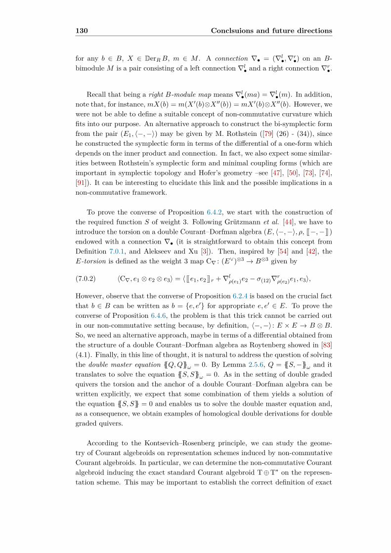
130 Conclsuions and future directions
for any b ∈ B, X ∈ DerRB, m ∈ M . A connection ∇• = (∇l•,∇r•) on an B-bimodule M is a pair consisting of a left connection ∇l• and a right connection ∇r•.
Recall that being a right B-module map means ∇l•(ma) = ∇l•(m). In addition,note that, for instance,mX(b) = m(X ′(b)⊗X ′′(b)) = mX ′(b)⊗X ′′(b). However, wewere not be able to define a suitable concept of non-commutative curvature whichfits into our purpose. An alternative approach to construct the bi-symplectic formfrom the pair (E1, 〈−,−〉) may be given by M. Rothstein ([79] (26) - (34)), sincehe constructed the symplectic form in terms of the differential of a one-form whichdepends on the inner product and connection. In fact, we also expect some similar-ities between Rothstein’s symplectic form and minimal coupling forms (which areimportant in symplectic topology and Hofer’s geometry –see [47], [50], [73], [74],[91]). It can be interesting to elucidate this link and the possible implications in anon-commutative framework.
To prove the converse of Proposition 6.4.2, we start with the construction ofthe required function S of weight 3. Following Grützmann et al. [44], we have tointroduce the torsion on a double Courant–Dorfman algebra (E, 〈−,−〉, ρ, [[ −,− ]] )endowed with a connection ∇• (it is straightforward to obtain this concept fromDefinition 7.0.1, and Alekseev and Xu [3]). Then, inspired by [54] and [42], theE-torsion is defined as the weight 3 map C∇ : (E∨)⊗3 → B⊗3 given by
(7.0.2) 〈C∇, e1 ⊗ e2 ⊗ e3〉 = 〈 [[ e1, e2 ]] r +∇lρ(e1)e2 − σ(12)∇rρ(e2)e1, e3〉,
However, observe that the converse of Proposition 6.2.4 is based on the crucial factthat b ∈ B can be written as b = e, e′ for appropriate e, e′ ∈ E. To prove theconverse of Proposition 6.4.6, the problem is that this trick cannot be carried outin our non-commutative setting because, by definition, 〈−,−〉 : E × E → B ⊗ B.So, we need an alternative approach, maybe in terms of a differential obtained fromthe structure of a double Courant–Dorfman algebra as Roytenberg showed in [83](4.1). Finally, in this line of thought, it is natural to address the question of solvingthe double master equation Q,Qω = 0. By Lemma 2.5.6, Q = S,−ω and ittranslates to solve the equation S, Sω = 0. As in the setting of double gradedquivers the torsion and the anchor of a double Courant–Dorfman algebra can bewritten explicitly, we expect that some combination of them yields a solution ofthe equation S, S = 0 and enables us to solve the double master equation and,as a consequence, we obtain examples of homological double derivations for doublegraded quivers.
According to the Kontsevich–Rosenberg principle, we can study the geome-try of Courant algebroids on representation schemes induced by non-commutativeCourant algebroids. In particular, we can determine the non-commutative Courantalgebroid inducing the exact standard Courant algebroid T⊕T∗ on the represen-tation scheme. This may be important to establish the correct definition of exact

Conclsuions and future directions 131
non-commutative Courant algebroid, or transitive non-commutative Courant alge-broids (recall that a Courant algebroid is transitive if its anchor is surjective), andto study some of their properties. In particular, we may obtain a non-commutativeanalogue of the Ševera class, a “curvature 3-form” classifying non-commutativeexact Courant algebroids.
Furthermore, it is a classical topic in geometry that, in presence of a symmetry,a given geometrical structure may, under suitable conditions, pass to the quotient.H. Bursztyn, G. R. Cavalcanti and M. Gualtieri [17] presented a theory of reduc-tion for exact Courant algebroids, which can be regarded as an “odd” analog ofthe usual notion of symplectic reduction due to Marsden and Weinstein. In fact,Burzstyn et al. specialize the reduction procedure when a moment map is involved.The idea is to translate this procedure to the non-commutative framework, usingthe non-commutative moment map given by Crawley-Boevey–Etingof–Ginzburg[30] §4.1 in terms of the distinguished double derivation ∆.
Finally, roughly speaking, higher Courant algebroids are analogues to Courantalgebroids whose operations (the inner product and the higher-order Courant–Dorfman bracket) take place on the direct sum bundle TM ⊕
∧n T∗M , with Ma fixed C∞-manifold. In his ongoing thesis, Camilo Rengifo provides a naturalcontext for the study of higher Courant algebroids in the framework of differentialgraded geometry. Therefore, we can study whether the tools developed in thisthesis can be applied to define “higher non-commutative Courant algebroids”satisfying the Kontsevich–Rosenberg principle, and if we can obtain examples ofthese structures using double graded quivers.


Chapter 8
Conclusiones y direcciones futuras
En esta tesis, los carcajs graduados doblados y las álgebras de caminos gradu-adas proporcionan un contexto natural para validar la teoría y las herramientasintroducidas. En particular, probamos el Teorema 3.3.40 usando la descripción ex-plícita de la forma bi-simpléctica canónica sobre un quiver graduado doblado (verProposición 3.3.34). De todas formas, esperamos que el Teorema 3.3.40 se puedaprobar para N-álgebras tensoriales bi-simplécticas de peso 2 que no procedan decarcajs.
Una cuestión natural que ha surgido en esta tesis es probar el recíproco delTeorema 6.4.8. Siguiendo a Roytenberg [81] y como muestra la estructura de estatesis, esta pregunta se puede descomponer en diferentes resultados, interesantespor derecho propio. A partir de ahora, sea R un álgebra asociativa semisimple dedimensión finita sobre k, un cuerpo de característica cero. Además, a partir deahora consideraremos B como una R-álgebra asociativa. En primer lugar, paraclasificar N-álgebras tensoriales bi-simplécticas de peso 2 en términos de pares(E1, 〈−,−〉), siguiendo a Rothstein [79] (también a Roytenberg [81]), precisaremosde la noción de curvatura no conmutativa. Por ello, comenzamos buscando elconcepto de conexión en términos dobles derivaciones. En el curso de este trabajo,definimos estos objetos motivados por la definición dada por J. Cuntz y D. Quillen[31] §8 (inspirada en la de Connes expuesta en [24]):
Definition 8.0.1. SeaM un B-bimódulo. Una conexión por la izquierda ∇• sobreM es una aplicación de B-módulos por la derecha
∇l• : DerRB ×M −→ B ⊗M : (X,m) 7−→ ∇lXm,
satisfaciendo∇lX(bm) = b∇lX(m) +X(b)m,
para todo b ∈ B, X ∈ DerRB, m ∈ M . De manera análoga, una conexión por laderecha ∇• sobre M es una aplicación de B-módulos por la izquierda
∇r• : DerRB ×M −→M ⊗B : (X,m) 7−→ ∇rXm,
133

134 Conclusiones y direcciones futuras
tal que∇rX(mb) = ∇rX(m)b+mX(b)
para todo b ∈ B, X ∈ DerRB, m ∈ M . Una conexión ∇• = (∇l•,∇r•) sobre unB-bimódulo M es un par consistente en una conexión por la izquierda ∇l• y unaconexión por la derecha ∇r•.
Recordemos que ser una aplicación de B-módulos por la derecha significa∇l•(ma) = ∇l•(m). Además, observamos que, por ejemplo, mX(b) = m(X ′(b) ⊗X ′′(b)) = mX ′(b) ⊗ X ′′(b). De todas formas, no hemos sido capaces de encon-trar un concepto adecuado de curvatura no conmutativa que encaje en nuestropropósito. Un enfoque alternativo para construir la forma bi-simpléctica a partirdel par (E1, 〈−,−〉) se puede encontrar en el artículo de M. Rothstein ([79] (26)- (34)) ya que en él Rothstein construye la forma simpléctica en términos de ladiferencial de una 1-forma que depende de un producto escalar y de una conexión.De hecho, esperamos encontrar similitudes entre la forma simpléctica de Rothsteiny las formas minímamente acopladas (minimal coupling forms) que han resultadoser importantes en topología simpléctica y en la geometría de Hofer -ver [47], [50],[73], [74], [91]-). También puede ser interesante dilucidar esta conexión y las posi-bles implicaciones en un contexto no conmutativo.
Para probar el recíproco de la Proposición 6.4.2 empezamos con la construcciónde la necesaria función S de peso 3. Sigiuiendo a Grützmann et al. [44]tenemos que introducir la torsión sobre un álgebra de Courant–Dorfman doble(E, 〈−,−〉, ρ, [[ −,− ]] ) dotada con una conexión ∇• (es fácil obtener este conceptoa partir de la Definición 7.0.1, y Alexseeev y Xu [3]). Entonces, inspirados por[54] y [42], la E-torsión se define como la aplicación de peso 3 C∇ : (E∨)⊗3 → B⊗3
dada por
(8.0.2) 〈C∇, e1 ⊗ e2 ⊗ e3〉 = 〈 [[ e1, e2 ]] r +∇lρ(e1)e2 − σ(12)∇rρ(e2)e1, e3〉,
De todas formas, observamos que el recíproco de la Proposición 6.2.4 se basa en elhecho importante de que b ∈ B se puede escribir como b = e, e′ para e, e′ ∈ Eapropiados. Para probar el recíproco de la Proposición 6.4.6, el problema es queeste truco no se se puede usar en nuestro contexto no conmutativo porque, pordefinición, 〈−,−〉 : E × E → B ⊗ B. Luego precisamos un enfoque alternativo,quizás en términos de una diferencial obtenida a partir de la estructura de un álge-bra de Courant–Dorfman doble como Roytenberg mostró en [83] (4.1). Finalmente,en esta línea, es natural plantearse la cuestión de resolver la ecuación maestra dobleQ,Qω = 0. Por el Lema 2.5.6, Q = S,−ω y esto nos lleva a querer resolverla ecuación S, Sω = 0. Como en el contexto de carcajs graduados doblados latorsión y el ancla de un álgebra de Courant–Dorfman doble se puede escribir entérminos muy explícitos, esperamos que alguna combinación de estos objetos nosproporcione una solución de la ecuación S, S = 0 y, como consecuencia, obtenerejemplos de derivaciones dobles homológicas para carcajs dobles graduados.

Conclusiones y direcciones futuras 135
De acuerdo con el principio de Kontsevich–Rosenberg, podemos estudiar lageometría de los algebroides de Courant sobre los esquemas de representacionesinducidos por los algebroides de Courant no conmutativos. En particular, pode-mos determinar el algebroide de Courant no conmutativo que induce el algebroidede Courant estándar T⊕T∗ sobre los esquemas de representaciones. Esto puedeser importante para establecer la definición correcta de algebroides de Courantno conmutativos exactos o algebroides de Courant no conmutativos transitivos(recordemos que un algebroide de Courant es transitivo si su ancla es sobreyec-tiva), y para estudiar algunas de sus propiedades. En particular, podemos obtenerun análogo no conmutativo de la clase de Ševera, una “3-forma de curvatura” queclasifique los algebroides de Courant no conmutativos exactos.
Además, es un tema clásico en geometría que, en presencia de una simetría,una estructura geométrica dada, bajo condiciones adecuadas, puede descender alcociente. H. Bursztyn, G. R. Cavalcanti and M. Gualtieri [17] presentaron unateoría de reducción para algebroides de Courant exactos, que se puede ver como unanálogo “extraño” de la noción usual de reducción simpléctica debida a Marsden y aWeinstein. De hecho, Burzstyn et al. especializaron el procedimiento de reducciónen presencia de una aplicación momento. La idea es traducir este procedimientoal contexto no conmutativo, usando la aplicación momento no conmutativa dadapor Crawley-Boevey–Etingof–Ginzburg [30] §4.1 en términos de la doble derivacióndistinguida ∆.
Finalmente, en téerminos poco rigurosos, podemos decir que los algebroidesde Courant de orden superior son análogos a los algebroides de Courant cuyasoperaciones (el producto escalar y el corchete de Courant–Dorfman de ordensuperior) tienen lugar sobre el fibrado TM ⊕
∧n T∗M , con M una C∞-variedad.En su tesis en curso, Camilo Rengifo construye un contexto natural para el estudiode los algebroides de Courant de orden superior usando geometría diferencialgraduada. Por tanto, podemos estudiar si las herramientas desarrolladas en estatesis pueden ser útiles para definir ”algebroides de Courant de orden superior noconmutativos” satisfaciendo el principio de Kontsevich–Rosenberg, y si se puedenobtener ejemplos de estas estructuras usando carcajs graduados dobles.


Bibliography
[1] M. M. Abbasirad. Homotopy Theory of Differential Graded Modules andAdjoints of Restriction of Scalars. PhD thesis, The University of Sheffield.
[2] Füsun Akman. On some generalizations of Batalin-Vilkovisky algebras. J.Pure Appl. Algebra, 120(2):105–141, 1997.
[3] Anton Alekseev and Ping Xu. Derived Brackets and Courant Algebroidshttp://www.math.psu.edu/ping/anton-final.pdf.
[4] M. Alexandrov, A. Schwarz, O. Zaboronsky, and M. Kontsevich. Thegeometry of the master equation and topological quantum field theory.Internat. J. Modern Phys. A, 12(7):1405–1429, 1997.
[5] J. Alm. Universal algebraic structures on polyvector fields. PhD thesis,Stockholm University.
[6] Björn Andreas and Mario Garcia-Fernandez. Solutions of the Stromingersystem via stable bundles on Calabi-Yau threefolds. Comm. Math. Phys.,315(1):153–168, 2012.
[7] Ibrahim Assem, Daniel Simson, and Andrzej Skowroński. Elements ofthe representation theory of associative algebras. Vol. 1, volume 65 ofLondon Mathematical Society Student Texts. Cambridge University Press,Cambridge, 2006. Techniques of representation theory.
[8] M. F. Atiyah. Complex analytic connections in fibre bundles. Trans. Amer.Math. Soc., 85:181–207, 1957.
[9] Maurice Auslander, Idun Reiten, and Sverre O. Smalø. Representation theoryof Artin algebras, volume 36 of Cambridge Studies in Advanced Mathematics.Cambridge University Press, Cambridge, 1995.
[10] I. A. Batalin and G. A. Vilkovisky. Gauge algebra and quantization. Phys.Lett. B, 102(1):27–31, 1981.
[11] D. J. Benson. Representations and cohomology. II, volume 31 of CambridgeStudies in Advanced Mathematics. Cambridge University Press, Cambridge,second edition, 1998. Cohomology of groups and modules.
137

138 Bibliography
[12] Yuri Berest, Xiaojun Chen, Farkhod Eshmatov, and Ajay Ramadoss.Noncommutative Poisson structures, derived representation schemes andCalabi-Yau algebras. In Mathematical aspects of quantization, volume 583 ofContemp. Math., pages 219–246. Amer. Math. Soc., Providence, RI, 2012.
[13] Yuri Berest, Giovanni Felder, and Ajay Ramadoss. Derived representationschemes and noncommutative geometry. In Expository lectures on represen-tation theory, volume 607 of Contemp. Math., pages 113–162. Amer. Math.Soc., Providence, RI, 2014.
[14] Yuri Berest, George Khachatryan, and Ajay Ramadoss. Derived representa-tion schemes and cyclic homology. Adv. Math., 245:625–689, 2013.
[15] George M. Bergman. Coproducts and some universal ring constructions.Trans. Amer. Math. Soc., 200:33–88, 1974.
[16] Raf Bocklandt, Travis Schedler, and Michael Wemyss. Superpotentials andhigher order derivations. J. Pure Appl. Algebra, 214(9):1501–1522, 2010.
[17] Henrique Bursztyn, Gil R. Cavalcanti, and Marco Gualtieri. Reductionof Courant algebroids and generalized complex structures. Adv. Math.,211(2):726–765, 2007.
[18] Ana Cannas da Silva. Lectures on symplectic geometry, volume 1764 ofLecture Notes in Mathematics. Springer-Verlag, Berlin, 2001.
[19] Henri Cartan and Samuel Eilenberg. Homological algebra. PrincetonLandmarks in Mathematics. Princeton University Press, Princeton, NJ, 1999.With an appendix by David A. Buchsbaum, Reprint of the 1956 original.
[20] Alberto S. Cattaneo and Florian Schätz. Introduction to supergeometry. Rev.Math. Phys., 23(6):669–690, 2011.
[21] Gil R. Cavalcanti and Marco Gualtieri. Generalized complex geometry and T -duality. In A celebration of the mathematical legacy of Raoul Bott, volume 50of CRM Proc. Lecture Notes, pages 341–365. Amer. Math. Soc., Providence,RI, 2010.
[22] Ionuţ Ciocan-Fontanine and Mikhail Kapranov. Derived Quot schemes. Ann.Sci. École Norm. Sup. (4), 34(3):403–440, 2001.
[23] P. M. Cohn. Rings of fractions. Amer. Math. Monthly, 78:596–615, 1971.
[24] Alain Connes. Noncommutative differential geometry. Inst. Hautes ÉtudesSci. Publ. Math., (62):257–360, 1985.
[25] Ted Courant and Alan Weinstein. Beyond Poisson structures. In Actionhamiltoniennes de groupes. Troisième théorème de Lie (Lyon, 1986), vol-ume 27 of Travaux en Cours, pages 39–49. Hermann, Paris, 1988.

Bibliography 139
[26] Theodore James Courant. Dirac Manifolds. PhD thesis, University ofCalifornia at Berkeley.
[27] Theodore James Courant. Dirac manifolds. Trans. Amer. Math. Soc.,319(2):631–661, 1990.
[28] William Crawley-Boevey. Preprojective algebras, differential operators anda Conze embedding for deformations of Kleinian singularities. Comment.Math. Helv., 74(4):548–574, 1999.
[29] William Crawley-Boevey. Geometry of the moment map for representationsof quivers. Compositio Math., 126(3):257–293, 2001.
[30] William Crawley-Boevey, Pavel Etingof, and Victor Ginzburg. Noncommu-tative geometry and quiver algebras. Adv. Math., 209(1):274–336, 2007.
[31] Joachim Cuntz and Daniel Quillen. Algebra extensions and nonsingularity.J. Amer. Math. Soc., 8(2):251–289, 1995.
[32] Paul A. M. Dirac. Lectures on quantum mechanics, volume 2 of BelferGraduate School of Science Monographs Series. Belfer Graduate School ofScience, New York; produced and distributed by Academic Press, Inc., NewYork, 1967. Second printing of the 1964 original.
[33] Irene Dorfman. Dirac structures and integrability of nonlinear evolutionequations. Nonlinear Science: Theory and Applications. John Wiley & Sons,Ltd., Chichester, 1993.
[34] Irene Ya. Dorfman. Dirac structures of integrable evolution equations. Phys.Lett. A, 125(5):240–246, 1987.
[35] Pavel Etingof, Oleg Golberg, Sebastian Hensel, Tiankai Liu, Alex Schwend-ner, Dmitry Vaintrob, and Elena Yudovina. Introduction to representationtheory, volume 59 of Student Mathematical Library. American MathematicalSociety, Providence, RI, 2011. With historical interludes by Slava Gerovitch.
[36] Daniel R. Farkas and Gail Letzter. Ring theory from symplectic geometry.J. Pure Appl. Algebra, 125(1-3):155–190, 1998.
[37] Peter Gabriel. Unzerlegbare Darstellungen. I. Manuscripta Math., 6:71–103;correction, ibid. 6 (1972), 309, 1972.
[38] Peter Gabriel. Indecomposable representations. II. In Symposia Mathematica,Vol. XI (Convegno di Algebra Commutativa, INDAM, Rome, 1971), pages81–104. Academic Press, London, 1973.
[39] Pierre Gabriel. Des catégories abéliennes. Bull. Soc. Math. France, 90:323–448, 1962.
[40] Victor Ginzburg. Calabi–Yau algebras arXiv : 0612139v3.

140 Bibliography
[41] Victor Ginzburg. Lectures on Noncommutative GeometryarXiv:math.AG/0506603.
[42] Victor Ginzburg and Travis Schedler. Differential operators and BVstructures in noncommutative geometry. Selecta Math. (N.S.), 16(4):673–730, 2010.
[43] Alexander Grothendieck. Sur quelques points d’algèbre homologique. TôhokuMath. J. (2), 9:119–221, 1957.
[44] Melchior Grützmann, Jean-Philippe Michel, and Ping Xu. Weyl quantizationof degree 2 symplectic graded manifolds arXiv:1410.3346v1.
[45] Marco Gualtieri. Generalized complex geometry. PhD thesis, University ofOxford.
[46] Marco Gualtieri. Branes on Poisson varieties. In The many facets of geometry,pages 368–394. Oxford Univ. Press, Oxford, 2010.
[47] Victor Guillemin, Eugene Lerman, and Shlomo Sternberg. Symplectic fibra-tions and multiplicity diagrams. Cambridge University Press, Cambridge,1996.
[48] Robin Hartshorne. Algebraic geometry. Springer-Verlag, New York-Heidelberg, 1977. Graduate Texts in Mathematics, No. 52.
[49] Nigel Hitchin. Generalized Calabi-Yau manifolds. Q. J. Math., 54(3):281–308, 2003.
[50] Helmut Hofer and Eduard Zehnder. Symplectic invariants and Hamiltoniandynamics. Modern Birkhäuser Classics. Birkhäuser Verlag, Basel, 2011.Reprint of the 1994 edition.
[51] Rolf Källström. Smooth modules over Lie algebroids I arXiv:9808108v1.
[52] Mikhail Kapranov. Free Lie algebroids and the space of paths. Selecta Math.(N.S.), 13(2):277–319, 2007.
[53] Bernhard Keller. Deformed Calabi-Yau completions. J. Reine Angew. Math.,654:125–180, 2011. With an appendix by Michel Van den Bergh.
[54] Frank Keller and Stefan Waldmann. Formal deformations of Dirac structures.J. Geom. Phys., 57(3):1015–1036, 2007.
[55] Frank Keller and Stefan Waldmann. Deformation theory of Courantalgebroids via the Rothstein algebra. J. Pure Appl. Algebra, 219(8):3391–3426, 2015.
[56] G. A. Khachatryan. Derived Representation Schemes and Non-commutativeGeometry. PhD thesis, Cornell University, 2012.
Bibliography 141
[57] Masoud Khalkhali. Basic noncommutative geometry. EMS Series of Lecturesin Mathematics. European Mathematical Society (EMS), Zürich, 2009.
[58] Maxim Kontsevich. Formal (non)commutative symplectic geometry. InThe Gel′fand Mathematical Seminars, 1990–1992, pages 173–187. BirkhäuserBoston, Boston, MA, 1993.
[59] Maxim Kontsevich and Alexander L. Rosenberg. Noncommutative smoothspaces. In The Gelfand Mathematical Seminars, 1996–1999, Gelfand Math.Sem., pages 85–108. Birkhäuser Boston, Boston, MA, 2000.
[60] Y. Kosmann-Schwarzbach and K. C. H. Mackenzie. Differential operatorsand actions of Lie algebroids. In Quantization, Poisson brackets and beyond(Manchester, 2001), volume 315 of Contemp. Math., pages 213–233. Amer.Math. Soc., Providence, RI, 2002.
[61] Yvette Kosmann-Schwarzbach. Derived brackets. Lett. Math. Phys., 69:61–87, 2004.
[62] Yvette Kosmann-Schwarzbach. Courant algebroids. A short history. SIGMASymmetry Integrability Geom. Methods Appl., 9:Paper 014, 8, 2013.
[63] Alexei Kotov and Thomas Strobl. Generalizing geometry—algebroidsand sigma models. In Handbook of pseudo-Riemannian geometry andsupersymmetry, volume 16 of IRMA Lect. Math. Theor. Phys., pages 209–262. Eur. Math. Soc., Zürich, 2010.
[64] T. Y. Lam. Lectures on modules and rings, volume 189 of Graduate Texts inMathematics. Springer-Verlag, New York, 1999.
[65] T. Y. Lam. Introduction to quadratic forms over fields, volume 67 of GraduateStudies in Mathematics. American Mathematical Society, Providence, RI,2005.
[66] T. Y. Lam. Exercises in modules and rings. Problem Books in Mathematics.Springer, New York, 2007.
[67] Calin Iuliu Lazaroiu. On the non-commutative geometry of topological D-branes. J. High Energy Phys., (11):032, 57 pp. (electronic), 2005.
[68] David Li-Bland and Eckhard Meinrenken. Courant algebroids and Poissongeometry. Int. Math. Res. Not. IMRN, (11):2106–2145, 2009.
[69] David Li-Bland and Pavol Ševera. Integration of exact Courant algebroids.Electron. Res. Announc. Math. Sci., 19:58–76, 2012.
[70] Zhang-Ju Liu, Alan Weinstein, and Ping Xu. Manin triples for Liebialgebroids. J. Differential Geom., 45(3):547–574, 1997.
[71] Saunders Mac Lane. Homology. Classics in Mathematics. Springer-Verlag,Berlin, 1995. Reprint of the 1975 edition.

142 Bibliography
[72] Hideyuki Matsumura. Commutative ring theory, volume 8 of CambridgeStudies in Advanced Mathematics. Cambridge University Press, Cambridge,second edition, 1989. Translated from the Japanese by M. Reid.
[73] Dusa McDuff. Introduction to symplectic topology. In Symplectic geometryand topology (Park City, UT, 1997), volume 7 of IAS/Park City Math. Ser.,pages 5–33. Amer. Math. Soc., Providence, RI, 1999.
[74] L. Polterovich. Gromov’s K-area and symplectic rigidity. Geom. Funct.Anal., 6(4):726–739, 1996.
[75] Daniel Quillen. Algebra cochains and cyclic cohomology. Inst. Hautes ÉtudesSci. Publ. Math., (68):139–174 (1989), 1988.
[76] Alexander Rosenberg. Selected Papers on Noncommutative Geometryhttp://newprairiepress.org/ebooks/1//nag.pdf. 2014.
[77] Alexander L. Rosenberg. Noncommutative algebraic geometry and represen-tations of quantized algebras, volume 330 ofMathematics and its Applications.Kluwer Academic Publishers Group, Dordrecht, 1995.
[78] Alexander L. Rosenberg. Noncommutative schemes. Compositio Math.,112(1):93–125, 1998.
[79] Mitchell Rothstein. The structure of supersymplectic supermanifolds. InDifferential geometric methods in theoretical physics (Rapallo, 1990), volume375 of Lecture Notes in Phys., pages 331–343. Springer, Berlin, 1991.
[80] Dmitry Roytenberg. Courant algebroids, derived brackets and even symplecticsupermanifolds. PhD thesis, University of California at Berkeley.
[81] Dmitry Roytenberg. On the structure of graded symplectic supermanifoldsand Courant algebroids. In Quantization, Poisson brackets and beyond(Manchester, 2001), volume 315 of Contemp. Math., pages 169–185. Amer.Math. Soc., Providence, RI, 2002.
[82] Dmitry Roytenberg. AKSZ-BV formalism and Courant algebroid-inducedtopological field theories. Lett. Math. Phys., 79(2):143–159, 2007.
[83] Dmitry Roytenberg. Courant-Dorfman algebras and their cohomology. Lett.Math. Phys., 90(1-3):311–351, 2009.
[84] William F. Schelter. Smooth algebras. J. Algebra, 103(2):677–685, 1986.
[85] Albert Schwarz. Geometry of Batalin-Vilkovisky quantization. Comm. Math.Phys., 155(2):249–260, 1993.
[86] J.-P. Serre. Modules projectifs et espaces fibrés à fibre vectorielle. InSéminaire P. Dubreil, M.-L. Dubreil-Jacotin et C. Pisot, 1957/58, Fasc. 2,Exposé 23, page 18. Secrétariat mathématique, Paris, 1958.

Bibliography 143
[87] Jean-Pierre Serre. Faisceaux algébriques cohérents. Ann. of Math. (2),61:197–278, 1955.
[88] Pavol Ševera. CA = symplectic dg-manifold with sym-plectic form of degree 2; the connection between CAs andgerbes via dg manifolds. Letters to A. Weinstein (1998–2000).http://sophia.dtp.fmph.uniba.sk/ severa/letters/.
[89] Pavol Ševera. Some title containing the words “homotopy” and “symplectic”,e.g. this one. In Travaux mathématiques. Fasc. XVI, Trav. Math., XVI, pages121–137. Univ. Luxemb., Luxembourg, 2005.
[90] Pavol Ševera and Alan Weinstein. Poisson geometry with a 3-form back-ground. Progr. Theoret. Phys. Suppl., (144):145–154, 2001. Noncommutativegeometry and string theory (Yokohama, 2001).
[91] Shlomo Sternberg. Minimal coupling and the symplectic mechanics of aclassical particle in the presence of a Yang-Mills field. Proc. Nat. Acad. Sci.U.S.A., 74(12):5253–5254, 1977.
[92] Richard G. Swan. Vector bundles and projective modules. Trans. Amer.Math. Soc., 105:264–277, 1962.
[93] Robert M. Thrall. On ahdir algebras. Bull. Amer. Math. Soc.., 53(1):p684,1947.
[94] A. Yu. Vaıntrob. Lie algebroids and homological vector fields. Uspekhi Mat.Nauk, 52(2(314)):161–162, 1997.
[95] Michel Van den Bergh. Blowing up of non-commutative smooth surfaces.Mem. Amer. Math. Soc., 154(734):x+140, 2001.
[96] Michel Van den Bergh. Double Poisson algebras. Trans. Amer. Math. Soc.,360(11):5711–5769, 2008.
[97] Michel Van den Bergh. Non-commutative quasi-Hamiltonian spaces. InPoisson geometry in mathematics and physics, volume 450 of Contemp.Math., pages 273–299. Amer. Math. Soc., Providence, RI, 2008.
[98] Michel Van den Bergh. Calabi-Yau algebras and superpotentials. SelectaMath. (N.S.), 21(2):555–603, 2015.
[99] Theodore Voronov. Graded manifolds and Drinfeld doubles for Lie bialge-broids. In Quantization, Poisson brackets and beyond (Manchester, 2001),volume 315 of Contemp. Math., pages 131–168. Amer. Math. Soc., Provi-dence, RI, 2002.
[100] Charles A. Weibel. An introduction to homological algebra, volume 38 ofCambridge Studies in Advanced Mathematics. Cambridge University Press,Cambridge, 1994.