the net reclassification index (nri): a misleading measure

UW Biostatistics Working Paper Series

3-19-2013

The Net Reclassification Index (NRI): aMisleading Measure of Prediction Improvementwith Miscalibrated or Overfit ModelsMargaret PepeUniversity of Washington, Fred Hutch Cancer Research Center, [email protected]

Jin FangFred Hutch Cancer Research Center, [email protected]

Ziding FengUniversity of Washington & Fred Hutchinson Cancer Research Center, [email protected]

Thomas GerdsUniversity of Copenhagen, [email protected]

Jorgen HildenUniversity of Copenhagen, [email protected]

This working paper is hosted by The Berkeley Electronic Press (bepress) and may not be commercially reproduced without the permission of thecopyright holder.Copyright © 2011 by the authors

Suggested CitationPepe, Margaret; Fang, Jin; Feng, Ziding; Gerds, Thomas; and Hilden, Jorgen, "The Net Reclassification Index (NRI): a MisleadingMeasure of Prediction Improvement with Miscalibrated or Overfit Models" (March 2013). UW Biostatistics Working Paper Series.Working Paper 392.http://biostats.bepress.com/uwbiostat/paper392

http://biostats.bepress.com/uwbiostat

1

D R A F T U N D E R R E V I E W

1. Introduction

The Net Reclassification Index (NRI) was introduced in 2008 (Pencina and others, 2008) as a

new statistic to measure the improvement in prediction performance gained by adding a marker,

Y , to a set of baseline predictors, X, for predicting a binary outcome, D. The statistic has gained

huge popularity in the applied biomedical literature. On March 13, 2013 through a search with

Google Scholar we found 840 papers (44 since January 2012) that contained the acronym ‘NRI’

and referenced Pencina and others (2008). The measure has been extended from its original

formulation (Pencina and others, 2010; Li and others, 2012). In this note we demonstrate a

fundamental problem with use of the NRI in practice. We refer to work by Hilden and Gerds

(2013) that provides insight into the source of the problems.

2. Illustration with Simulated Data

Consider a study that fits the baseline model risk(X) = P (D = 1|X) and the expanded model

risk(X, Y ) = P (D = 1|X, Y ) using a training dataset. The fitted models that we denote by

ˆrisk(X) and ˆrisk(X, Y ) are then evaluated and compared in a test dataset. The continuous NRI

statistic (Pencina and others, 2010) is calculated as

NRI = 2{P [ ˆrisk(X, Y ) > ˆrisk(X)|D = 1] − P [ ˆrisk(X, Y ) > ˆrisk(X)|D = 0]} (2.1)

the proportion of cases in the test dataset for whom ˆrisk(X, Y ) > ˆrisk(X) minus the corresponding

proportion of controls, multiplied by 2.

We generated data from a very simple simulation model described in the Supplementary

Materials where X and Y are univariate and the logistic regression models hold:

Hosted by The Berkeley Electronic Press

2

logitP (D = 1|X) = α0 + α1X (2.2)

logitP (D = 1|X, Y ) = β0 + β1X + β2Y . (2.3)

We used a small training set and fit logistic regression models of the correct forms in (2.2)

and (2.3). Using a large test dataset we calculated the continuous NRI statistic for the training

set derived models:

logit ˆrisk(X) = α̂0 + α̂1X

logit ˆrisk(X, Y ) = β̂0 + β̂1X + β̂2Y .

The data were generated under the null scenario where Y does not add predictive information,

i.e., β2 = 0. The results in Table 1 indicate, however, that the NRI statistic is positive on average.

That is, the NRI statistic calculated on the test dataset tends to indicate the erroneous result

that Y contributes predictive information when in fact it does not.

We also calculated more traditional measures of performance improvement using their em-

pirical estimates in the test dataset: ∆AUC = AUC( ˆrisk(X, Y )) − AUC( ˆrisk(X)); ∆ROC(f) =

ROC(f, ˆrisk(X, Y )) − ROC(f, ˆrisk(X)); ∆SNB(t) = SNB(t, ˆrisk(X, Y )) − SNB(t, ˆrisk(X)) and

∆Brier = Brier( ˆrisk(X)) − Brier( ˆrisk(X, Y )) where

AUC(risk) = P (riskı > risk|Dı = 1, D = 0)

ROC(f, risk) = P (riskı > τ (f)|Dı = 1) where τ (f) : P (risk > τ (f)|D = 0) = f

SNB(t, risk) = P (risk > t|D = 1) − P (D = 0)

P (D = 1)

t

1 − tP (risk > t|D = 0)

Brier(risk) = E(D − risk)2.

http://biostats.bepress.com/uwbiostat/paper392

3

The AUC is the area under the receiver operating characteristic (ROC) curve. The ROC(f, risk)

measure is the proportion of cases classified as high risk when the high risk threshold is chosen as

that exceeded by no more than a proportion f of controls. The standardized net benefit, SNB(t),

is a weighted average of the true and false positive rates associated with use of the risk threshold

t to classify subjects as high risk. This is a measure known by various names in the literature,

including the decision curve (Vickers and Elkin, 2006) and the relative utility (Baker and others,

2009). The Brier score is a classic sum of squares measure. In simulation studies we set f = 0.2

for ∆ROC(f) and t = P [D = 1], the average risk, for ∆SNB(t).

In contrast to the NRI statistic, we found that changes in the two ROC based measures, the

standardized net benefit and the Brier score were negative on average in the test datasets, in

all simulation scenarios (Table 1). Negative values for measures of performance improvement in

the test dataset are appropriate because, given that Y is not predictive we expect that the fitted

model ˆrisk(X, Y ) is further from the true risk, P (D = 1|X), than is ˆrisk(X). In particular, the

model giving rise to ˆrisk(X) requires estimating only 2 parameters and takes advantage of setting

β2 at its true value, β2 = 0. In contrast, by fitting the three parameter model (2.3) that enters Y

as a predictor, we incorporate noise and variability into ˆrisk(X, Y ). The ∆Brier score, ∆ROC(f),

∆AUC and ∆SNB(t) quantify the disimprovement in the performance of ˆrisk(X, Y ) relative to

ˆrisk(X) in different ways. In contrast, the NRI statistic tends to mislead us into thinking that

the expanded model is an improvement over the baseline model.

3. Illustration with a Theoretical Example

Hilden and Gerds (2013) constructed some artificial examples of miscalibrated risk models and

showed in simulation studies that the NRI statistic can be misleading. We now consider a sim-

plified version of one of their examples and prove a theoretical large sample result. The example

provides some insight into the simulation study results. Specifically, let Y be a constant, Y = 0


4

say, and consider a model risk∗(X, Y ) that is a distorted version of the true baseline risk function

risk(X) but that contains no additional predictive information:

logit risk∗(X, Y ) = logit risk(X) + ε if risk(X) > ρ (3.4)

logit risk∗(X, Y ) = logit risk(X) − ε if risk(X) < ρ (3.5)

where ρ = P (D = 1). Result 1 below shows that the NRI > 0 for comparing the model

risk∗(X, Y ) with the baseline model risk(X). Here the training and test datasets are consid-

ered to be very large so there is no sampling variability, but the expanded model risk∗(X, Y ) is

clearly miscalibrated while the baseline model is not.

Result 1

Assume that the baseline model is not the null model,

P (risk(X) 6= ρ) > 0.

Then NRI > 0 for the model (3.4)-(3.5).

Proof

Since the baseline model is well calibrated and

P (D = 1|risk(X) > ρ) = E(risk(X)|risk(X) > ρ),

we have

P (D = 1|risk(X) > ρ) = ρ + δ for some δ > 0.


5

NRI =2 {P (risk∗(X, Y ) > risk(X)|D = 1) − P (risk∗(X, Y ) > risk(X)|D = 0)}

=2

{

P (D = 1|risk(X) > ρ)P (risk(X) > ρ)

P (D = 1)− P (D = 0|risk(X) > ρ)P (risk(X) > ρ)

P (D = 0)

}

=2P (risk(X) > ρ)

{

ρ + δ

ρ− 1 − ρ− δ

1 − ρ

}

=2P (risk(X) > ρ)

{

δ

ρ+

δ

1 − ρ

}

=2δP (risk(X) > ρ)

ρ(1 − ρ)> 0

�

We see that even in an infinitely large test dataset, the NRI associated with the expanded

model in (3.4)-(3.5) is positive despite the fact that the expanded model contains no more pre-

dictive information than the baseline model. The integrated discrimination improvement (IDI)

statistic was also proposed by Pencina and others (2008) and is quite widely used (Kerr and

others, 2011). Hilden and Gerds (2013) proved that the IDI> 0 for a different example of an

uninformed expanded model.

4. Further Results

The expanded model in Result 1 is an extreme form of a miscalibrated model. Similarly, in the

simulated data example, the expanded model derived from the small training dataset is likely to

be miscalibrated in the test dataset. This is due to the phenomenon of overfitting. Miscalibration

in the test dataset due to overfitting in the training set is likely to be exacerbated by inclusion

of multiple novel markers in the expanded model. We see in Table 2 that the effects on NRI are

more pronounced in the presence of multiple novel markers that are not predictive.

We next considered a scenario where a marker Y does add predictive information. The true

expanded model in Table 3 is

model(X, Y ) : logitP (D = 1|X, Y ) = β0 + β1X + β2Y .


6

We fit this model and a model with superfluous interaction term to the training data

model(X, Y, XY ) : logitP (D = 1|X, Y ) = γ0 + γ1X + γ2Y + γ3XY .

The test set NRIs comparing each of these fitted models with the fitted baseline model are

summarized in Table 3. For comparison we display the NRI calculated using the true risk model

parameter values. In some scenarios the NRI derived from the overfit model with interaction is

substantially larger than the true NRI. For example, when AUCX = 0.9 and AUCY = 0.7, the

average NRI is 39.92% compared with the true NRI of 28.41%.

Considering the fact that the models fit to training data should be observed to perform

worse than the true risk models, their tendency to appear better than the true risk models is

particularly disconcerting. We see from Table 3 that the ROC based measures, the Brier Score

and the net benefit all indicate that the performances of both of the expanded models fit to

training data are worse than the performance of the true risk model. Moreover, as expected, the

overfit model, model(X, Y, XY ), is generally shown to have worse performance than the model

without interaction. The NRI statistic however, only rarely conforms with this pattern. In five of

the six scenarios considered, the NRI statistic for the overfit model(X, Y, XY ) was larger than

that for the model(X, Y ). We conclude that miscalibration of the expanded model is problematic

not only when the new marker is uninformative but also when the new marker is informative. In

particular, overfitting can lead to inappropriately large values for the NRI in the test dataset.

5. Insights

Although we cannot fully explain why the NRI statistic tends to be large when the model for

risk(X, Y ) is overfit to training data, we can share a few relevant observations.

5.1 NRI is not a Proper Measure of Performance Improvement


7

Hilden and Gerds (2013) attribute the problem with the NRI statistic to the possibility that it is

not based on a ‘proper scoring rule.’ See Gneiting and Raftery (2007) for an in-depth discussion

of proper scoring rules.

In our context we need to expand on the definition of propriety. Let a population prediction

performance improvement measure (PIM) comparing r∗(X, Y ), a function of (X, Y ), to the true

baseline risk function r(X) = P (D = 1|X), be denoted by S:

PIM = S(r∗(X, Y ), r(X), F (D, X, Y ))

where F is the population distribution of (D, X, Y ).

Definition

The PIM is proper if for all F and r∗(X, Y ):

S(r(X, Y ), r(X), F (D, X, Y )) > S(r∗(X, Y ), r(X), F (D, X, Y )). (5.6)

In other words, a prediction improvement measure is proper if it is maximized at the true risk

function of (X, Y ), r(X, Y ) = P (D = 1|X, Y ). If the inequality in (5.6) is strict, then r(X, Y ) is

the unique function that maximizes S and the PIM is said to be strictly proper.

Propriety is generally considered a desirable attribute (Hilden and Gerds, 2013; Gneiting and

Raftery, 2007). An unquestionably appealing attribute of a proper PIM is that improvement

in performance cannot be due simply to disimprovement in calibration of the baseline model.

Result 1 proves with a counter example that the NRI is not proper because NRI > 0 with use

of the function risk∗(X, Y ) while NRI = 0 with use of the true risk function risk(X, Y ) that

in this example is the same as risk(X). On the other hand, it is well known from the theory of

least squares that the change in the Brier score is proper, a fact that follows from the equality

E(D|X, Y ) = risk(X, Y ). In addition, the ∆AUC and ∆ROC(f) measures are proper since the

ROC curve for (X, Y ) is maximized at all points by the risk function (McIntosh and Pepe, 2002).

Interestingly, these are not strictly proper measures because ROC curves are also maximized


8

by any monotone increasing function of the risk. We show in supplementary materials that the

change in the standardized net benefit, ∆SNB(t), is proper. Being proper measures of prediction

improvement appears to translate into more sensible comparisons of risk models in our simulation

studies. In particular, distortion of the baseline model by adding unnecessary predictors to the

model does not increase the estimated values of the proper performance measures but can increase

the NRI.

5.2 Manifestations of Overfitting

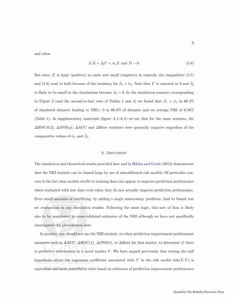
When risk models include superfluous predictor variables, predictions are apt to predict more

poorly than predictions derived from models without them. In Figure 1 we demonstrate this

for one simulated dataset corresponding to the scenario in the second-to-last row of Table 1.

Observe that the predictions from the baseline model, ˆrisk(X), are seen to be closer to the

true risk, risk(X), than are the more variable predictions based on ˆrisk(X, Y ), where Y is an

uninformative variable that is therefore superfluous. The NRI statistic does not acknowledge the

poorer predictions while the other performance improvement measures do (Figure 1 caption).

We compared the estimated odds ratios for X in the overfit models described in Table 2 with

that in the fitted baseline model. Results shown in Table 4 indicate that odds ratios are biased

too large in the overfit models. This presumably provides some rationale for use of shrinkage

techniques to address problems with overfitting (Hastie and others (2001), section 10.12.1). In-

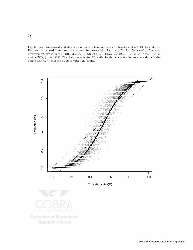
terestingly, when the odds ratio for X is larger in an overfit model than in the baseline model, the

NRI statistic is generally positive (Figure 2). We now provide some intuition for this observation.

Note that the NRI statistic compares ˆrisk(X, Y ) with ˆrisk(X) for each individual. Assuming that

the intercept terms center X at 0 but otherwise can be ignored, the NRI statistic adds positive

contributions when

β̂1X + β̂2Y > α̂1X and D = 1 (5.7)


9

and when

β̂1X + β̂2Y < α̂1X and D = 0. (5.8)

But since X is large (positive) in cases and small (negative) in controls, the inequalities (5.7)

and (5.8) tend to hold because of the tendency for β̂1 > α̂1. Note that Y is centered at 0 and β̂2

is likely to be small in the simulations because β2 = 0. In the simulation scenario corresponding

to Figure 2 (and the second-to-last rows of Tables 1 and 4) we found that β̂1 > α̂1 in 66.4%

of simulated datasets leading to NRI> 0 in 66.9% of datasets and an average NRI of 6.56%

(Table 1). In supplementary materials (figure A.1-A.4) we see that for the same scenario, the

∆ROC(0.2), ∆SNB(ρ), ∆AUC and ∆Brier statistics were generally negative regardless of the

comparative values of α̂1 and β̂1.

6. Discussion

The simulation and theoretical results provided here and in Hilden and Gerds (2013) demonstrate

that the NRI statistic can be biased large by use of miscalibrated risk models. Of particular con-

cern is the fact that models overfit to training data can appear to improve prediction performance

when evaluated with test data even when they do not actually improve prediction performance.

Even small amounts of overfitting, by adding a single unnecessary predictor, lead to biased test

set evaluations in our simulation studies. Following the same logic, this sort of bias is likely

also to be manifested in cross-validated estimates of the NRI although we have not specifically

investigated the phenomenon here.

In practice, one should not use the NRI statistic, or other prediction improvement performance

measures such as ∆AUC, ∆ROC(f), ∆SNB(t), or ∆Brier for that matter, to determine if there

is predictive information in a novel marker Y . We have argued previously that testing the null

hypothesis about the regression coefficient associated with Y in the risk model risk(X, Y ) is

equivalent and more powerful to tests based on estimates of prediction improvement performance


10

measures (Pepe and others, 2013).

On the other hand, for quantifying the improvement in prediction performance one must

choose summary statistics. There has been much debate in the literature about which measures

are most appropriate (Pepe and Janes, 2013). Arguments have centered on the interpretations

and clinical relevance of various measures. The results in this paper and in Hilden and Gerds

(2013) add another dimension to the debate. Regardless of the intuitive appeal that the NRI

statistic may garner, its potential for being inflated by miscalibrated or over-fit models is a very

serious concern.

Our results underscore the need to check model calibration as a crucial part of the exercise of

evaluating risk prediction models. In additional simulation studies (results not shown) we found

that after recalibrating the training set models to the test dataset, problems with inflated NRIs

were much reduced. However, guaranteeing well fitting risk models in practical applications is

not always possible. For this reason, other statistical measures of prediction improvement that

cannot be made large by miscalibration may be preferred for practical application. We especially

encourage use of the change in the standardized net benefit statistic and its components, the

changes in true and false positive rates, calculated at a relevant risk threshold, because, not only

is it a proper prediction improvement statistic, but it also quantifies prediction performance in

a clinically meaningful way (Pepe and Janes, 2013; Vickers and Elkin, 2006; Baker and others,

2009).

Acknowledgments

This work was supported in part by NIH grants R01 GM054438, U24 CA086368, and R01

CA152089.

Conflict of Interest: None declared.


11

Supplementary Material

Supplementary material is available online at http://biostatistics.oxfordjournals.org.


12 REFERENCES

References

Baker, Stuart G., Cook, Nancy R., Vickers, Andrew and Kramer, Barnett S.

(2009). Using relative utility curves to evaluate risk prediction. Journal of the Royal Statistical

Society: Series A (Statistics in Society) 172(4), 729–748.

Gneiting, Tilmann and Raftery, Adrian E. (2007). Strictly proper scoring rules, prediction,

and estimation. Journal of the American Statistical Association 102, 359–378.

Hastie, Trevor, Tibshirani, Robert and Friedman, J. H. (2001). The Elements of Sta-

tistical Learning: Data Mining, Inference, and Prediction. New York: Springer-Verlag.

Hilden, Jorgen and Gerds, Thomas A. (2013). Evaluating the impact of novel biomarkers:

Do not rely on IDI and NRI. Statistics in Medicine (in press).

Kerr, Kathleen F., McClelland, Robyn L., Brown, Elizabeth R. and Lumley,

Thomas. (2011). Evaluating the incremental value of new biomarkers with integrated dis-

crimination improvement. American Journal of Epidemiology 174(3), 364–374.

Li, Jialiang, Jiang, Binyan and Fine, Jason P. (2012, Nov). Multicategory reclassification

statistics for assessing improvements in diagnostic accuracy. Biostatistics (epub ahead of print).

McIntosh, Martin W. and Pepe, Margaret Sullivan. (2002, Sep). Combining several

screening tests: optimality of the risk score. Biometrics 58(3), 657–664.

Pencina, M.J., D’Agostino, R.B., D’Agostino, R.B. and Vasan, R.S. (2008). Evaluating

the added predictive ability of a new marker: from area under the ROC curve to reclassification

and beyond. Statistics in Medicine 27(2), 157–172. PMID: 17569110 PMCID: N/A; precedes

mandate.

Pencina, Michael J., D’Agostino, Ralph B. and Vasan, Ramachandran S. (2010, Dec).


REFERENCES 13

Statistical methods for assessment of added usefulness of new biomarkers. Clin Chem Lab

Med 48(12), 1703–1711.

Pepe, M.S. and Janes, H. (2013). Methods for Evaluating Prediction Performance of Biomark-

ers and Tests . In Risk Assessment and Evaluation of Predictions, Springer.

Pepe, MS, Kerr, KF, Longton, G and Wang, Z. (2013). Testing for improvement in pre-

diction model performance. Statistics in Medicine, Epub ahead of print. doi: 10.1002/sim.5727.

Vickers, A.J. and Elkin, E.B. (2006). Decision curve analysis: a novel method for evaluating

prediction models. Medical Decision Making 26(6), 565.


14

Tables and Figures

Table 1. Measures of improvement in prediction when risk models, logitP (D = 1|X) = α0 + α1X andlogitP (D = 1|X,Y ) = β0 + β1X + β2Y , are fit to a training dataset and applied to a test dataset. Thenovel marker Y does not improve prediction: the true models are linear logistic (2.2) and (2.3) withcoefficients: β2 = 0, β1 = α1 and β0 = α0. Performance measures are averaged over 1000 simulations.Data generation is described in Supplementary Materials

One Uninformative Marker

Simulation ScenarioPerformance Increment ×100

Average (standard error)

ρ = P (D = 1) AUCX1 N -training2 N -test3 NRI ∆ROC(0.2) ∆AUC ∆Brier ∆SNB(ρ)

0.1 0.6 250 25,000 0.27(0.09) −1.70(0.09) −1.28(0.08) −0.044(0.002) −1.85(0.12)0.1 0.7 250 25,000 1.38(0.16) −1.37(0.07) −0.86(0.05) −0.049(0.002) −1.31(0.07)0.1 0.8 250 25,000 3.22(0.28) −0.90(0.05) −0.48(0.02) −0.058(0.003) −0.80(0.04)0.1 0.9 250 25,000 7.72(0.52) −0.52(0.03) −0.25(0.01) −0.066(0.003) −0.57(0.03)0.5 0.6 50 5,000 0.57(0.15) −1.67(0.12) −1.19(0.11) −0.479(0.023) −1.69(0.15)0.5 0.7 50 5,000 2.78(0.28) −2.59(0.12) −1.69(0.08) −0.540(0.024) −2.49(0.13)0.5 0.8 50 5,000 6.56(0.47) −1.83(0.09) −1.00(0.05) −0.492(0.022) −1.62(0.08)0.5 0.9 50 5,000 17.09(0.91) −1.11(0.05) −0.56(0.03) −0.433(0.021) −1.17(0.06)

1Area under the ROC curve for the baseline model (X)

2Size of training dataset

3Size of test dataset


15

Table 2. Measures of improvement in prediction ×100 when risk models are fit to a training dataset of50 observations and assessed on a test dataset of 5000 observations where P (D = 1) = 0.5. The linearlogistic regression models fit to the training data are (i) baseline logitP (D = 1|X) = α0 + α1X ; (ii)model(X,Y1) : logitP (D = 1|X, Y1) = β0+β1X+β2Y1; (iii) model(X,Y1, Y2) : logitP (D = 1|X,Y1, Y2) =γ0 + γ1X + γ2Y1 + γ3Y2. Data generation is described in Supplementary Materials. Shown are averagesover 1000 simulations. Neither Y1 nor Y2 are informative — the true values of β2, γ2, and γ3 are zero.

Two Uninformative Markers

NRI ∆ROC(0.2) ∆AUC ∆ Brier ∆SNB(ρ)

Model (X,Y1) (X,Y1, Y2) (X,Y1) (X,Y1, Y2) (X,Y1) (X,Y1, Y2) (X,Y1) (X,Y1, Y2) (X,Y1) (X,Y1, Y2)

AUCX

0.60 0.61 0.78 −1.81 −2.91 −1.30 −2.18 −0.55 −1.12 −1.84 −3.060.70 2.08 3.63 −2.63 −4.55 −1.66 −2.95 −0.52 −1.08 −2.44 −4.360.80 6.18 10.60 −1.75 −3.50 −0.95 −1.89 −0.47 −0.96 −1.61 −3.140.90 17.83 28.00 −1.33 −2.57 −0.65 −1.27 −0.51 −1.03 −1.36 −2.63


16

Table 3. Measures of improvement in prediction when risk models are fit to a training dataset of N -training=50 observations and assessedon a test dataset of N -test=5000 observations where P (D = 1) = 0.5. The linear logistic regression models fit to the training datasets are(i) baseline logitP (D = 1|X) = α0 + α1X ; (ii) model(X,Y ) : logitP (D = 1|X, Y ) = β0 + β1X + β2Y ; (iii) model(X, Y, XY ) : logitP (D =1|X, Y ) = γ0 + γ1X + γ2Y + γ3XY . The marker Y is informative and the correct model is model(X,Y ) while the model(X, Y, XY ) is overfit.Data generation is described in Supplementary Materials. Shown are the true values of the performance measures (True) that use the true risk,as well as averages of estimated performance using training and test data over 1,000 simulations. All measures shown as %.

One Informative Marker

NRI ∆ROC(0.2) ∆AUC ∆Brier ∆SNB(ρ)

AUCX AUCY TrueModel(X,Y )

Model(X,Y,XY) True

Model(X, Y )

Model(X,Y,XY) True

Model(X,Y )

Model(X,Y,XY) True

Model(X,Y )

Model(X,Y,XY) True

Model(X,Y )

Model(X,Y,XY)

0.7 0.7 28.32 23.37 22.74 3.25 0.99 −0.89 1.98 0.64 −0.69 0.61 0.16 −0.41 3.21 0.98 −0.400.8 0.7 28.39 23.37 27.03 1.97 0.14 −1.13 1.03 0.06 −0.80 0.47 0.01 −0.45 1.84 0.15 −0.900.8 0.8 57.84 55.65 55.82 7.73 6.09 4.99 3.94 3.12 2.25 1.89 1.48 1.00 7.10 5.39 4.590.9 0.7 28.41 27.16 39.92 0.88 − 0.31 −1.15 0.43 −0.16 −0.77 0.29 −0.16 −0.59 0.92 −0.33 −1.250.9 0.8 57.87 57.13 63.05 3.40 2.31 1.61 1.69 1.14 0.53 1.19 0.74 0.30 3.79 2.49 1.710.9 0.9 89.58 87.02 88.18 7.35 6.46 5.59 3.74 3.23 2.54 2.81 2.40 1.95 8.85 7.50 6.74


17

Table 4. Average estimated odds ratios for X in models fit to training data generated using the samesettings as in Table 2. Both Y1 and Y2 are uninformative markers.

True Baseline Model Model (X,Y1) Model (X,Y1, Y2)

AUCX exp(α1) exp(α̂1) exp(β̂1) exp(γ̂1)

0.6 1.43 1.56 1.58 1.600.7 2.10 2.46 2.55 2.630.8 3.29 4.02 4.24 4.490.9 6.13 6.78∗ 7.37∗ 8.23∗

∗medians displayed when distribution is highly skewed


18

Fig. 1. Risk estimates calculated, using models fit to training data, on a test data set of 5000 observations.Data were simulated from the scenario shown in the second to last row of Table 1. Values of performanceimprovement statistics are: NRI= 33.95%, ∆ROC(0.2) = −1.65%, ∆AUC= −0.37%, ∆Brier= −0.54%and ∆SNB(ρ) = −1.77%. The thick curve is ˆrisk(X) while the thin curve is a lowess curve through thepoints ˆrisk(X, Y ) that are displaed with light circles.

��

��

��

��

��

��

��

��

��


19

Fig. 2. Scatterplots showing the relationship between the NRI statistic (×100) and β̂1 − α̂1 in 1000simulated datasets generated according to the scenario shown in the second to last row of Table 1. Thecoefficients are calculated by fitting the models logitP (D = 1|X) = α0 +α1X and logitP (D = 1|X, Y ) =β0 + β1X + β2Y to the training data. The NRI is calculated using the test dataset.

−0.5 0.0 0.5 1.0 1.5

−100

−50

05

01

00

α̂0 > β^

0

β^

1 − α̂1

NR

I×100

−0.5 0.0 0.5 1.0 1.5

−100

−50

05

01

00

α̂0 ≤ β^

0

β^

1 − α̂1

NR

I×100


A.1

SUPPLEMENTARY MATERIALS

A.1 Data Generation

The simulations reported in Table 1 are based on data generated as

(

X

Y

)

∼ N

((

µXD

0

)

,

(

1 00 1

))

where D is random binary variable with specified P (D = 1). We chose µX =√

2 Φ−1(AUCX) so

that the AUC for the baseline model was fixed by design.

Data for Table 2 were simulated as

X

Y1

Y2

∼ N

µXD

00

,

1 0 00 1 00 0 1

.

Data for Table 3 were generated from the distribution

(

X

Y

)

∼ N

((

µXD

µY D

)

,

(

1 00 1

))

where µX =√

2Φ−1(AUCX) and µY =√

2Φ−1(AUCY ).

A.2 Net Benefit is a Proper Scoring Statistic

Let X denote the available predictors and let r∗(X) and r(X) be two functions of X. Assume

that the true model is P (D = 1|X) = r(X) and the aim is to assess the decision rule based

on the model r∗(X) defined by r∗(X) > t. The standardized net benefit statistic at threshold t

associated with the function r∗(X) is

SNB(t, r∗(X)) = P (r∗(X) > t|D = 1) − 1 − ρ

ρ

t

1 − tP (r∗(X) > t|D = 0)


A.2

where ρ = P (D = 1). In terms of expectation over the marginal distribution of X, we write

ρSNB(t, r∗(X)) = E

{

I(r∗(X) > t, D = 1) − t

1 − tI(r∗(X) > t, D = 0)

}

= E

{

P (D = 1|X)I(r∗(X) > t) − t

1 − t[1− P (D = 1|X)]I(r∗(X) > t)

}

= E

{

I(r∗(X) > t)[r(X) − t

1 − t(1 − r(X))]

}

= E

{

I(r∗(X) > t)[r(X) − t

1 − t]

}

.

Now consider the difference between ρSNB(t, r(X)) and ρSNB(t, r∗(X)) : ρ(SNB(t, r(X)) −

SNB(t, r∗(X))) = 1

1−tE{(r(X) − t)(I(r(X) > t) − I(r∗(X)) > t))}

The entity inside the expectation, namely

(r(X) − t){I(r(X) > t) − I(r∗(X) > t)} (A.1)

is non-negative with probability 1. To see this, consider the various cases possible: (i) r(X) = t;

(ii) r(X) > t, r∗(X) > t; (iii) r(X) > t, r∗(X) < t (iv) r(X) < t, r∗(X) < t and (v) r(X) <

t, r∗(X) > t and observe that A.1 is > 0 in each case. Therefore the expectation is nonnegative.

In other words,

SNB(t, r(X))) > SNB(t, r∗(X))

for every function r∗(X). That is, SNB(t, r∗(X)) is maximized by r∗(X) = r(X), the true risk

function.


A.3

Figure A.1. Scatterplots showing the relationship between the ∆ROC(0.2) statistic (×100) and

β̂1−α̂1 in 1000 simulated datasets generated according to the scenario shown in the second to last

row of Table 1. The coefficients are calculated by fitting the models logitP (D = 1|X) = α0 +α1X

and logitP (D = 1|X, Y ) = β0 + β1X + β2Y to the training data. The ∆ROC(0.2) is calculated

using the test dataset.

−0.5 0.0 0.5 1.0 1.5

−4

0−

20

02

04

0

α̂0 > β^

0

β^

1 − α̂1

∆R

OC

(0.2

)*1

00

−0.5 0.0 0.5 1.0 1.5

−4

0−

20

02

04

0

α̂0 ≤ β^

0

β^

1 − α̂1

∆R

OC

(0.2

)*1

00


A.4

Figure A.2. Scatterplots showing the relationship between the ∆SNB(ρ) statistic (×100) and



and logitP (D = 1|X, Y ) = β0 + β1X + β2Y to the training data. The ∆SNB(ρ) is calculated

using the test dataset.

−0.5 0.0 0.5 1.0 1.5

−4

0−

20

02

04

0

α̂0 > β^

0

β^

1 − α̂1

∆S

NB

(ρ)*

10

0

−0.5 0.0 0.5 1.0 1.5

−4

0−

20

02

04

0

α̂0 ≤ β^

0

β^

1 − α̂1

∆S

NB

(ρ)*

10

0


A.5

Figure A.3. Scatterplots showing the relationship between the ∆AUC statistic (×100) and



and logitP (D = 1|X, Y ) = β0 + β1X + β2Y to the training data. The ∆AUC is calculated using

the test dataset.

−0.5 0.0 0.5 1.0 1.5

−3

0−

10

10

30

α̂0 > β^

0

β^

1 − α̂1

∆A

UC

*10

0

−0.5 0.0 0.5 1.0 1.5

−3

0−

10

10

30

α̂0 ≤ β^

0

β^

1 − α̂1

∆A

UC

*10

0


A.6

Figure A.4. Scatterplots showing the relationship between the ∆Brier statistic (×100) and



and logitP (D = 1|X, Y ) = β0 + β1X + β2Y to the training data. The ∆Brier is calculated using

the test dataset.

−0.5 0.0 0.5 1.0 1.5

−2

0−

10

01

02

0

α̂0 > β^

0

β^

1 − α̂1

∆B

rie

r*1

00

−0.5 0.0 0.5 1.0 1.5

−2

0−

10

01

02

0

α̂0 ≤ β^

0

β^

1 − α̂1

∆B

rie

r*1

00


the net reclassification index (nri): a misleading measure

Documents