the macroeconomic aggregates for england, 1209-2008 · the macroeconomic aggregates for england,...
TRANSCRIPT
The Macroeconomic Aggregates for England, 1209-2008 Gregory Clark, University of California, Davis ([email protected]) Revised Version - October 2009 UC Davis, Economics WP 09-19
Estimates are developed of the major macroeconomic aggregates – wages, land rents, interest rates, prices, factor shares, sectoral shares in output and employment, and real wages – for England by decade between 1209 and 2008. The efficiency of the economy 1209-2008 is also estimated. One finding is that the growth of real wages in the Industrial Revolution era and beyond was faster than the growth of output per person. Indeed until recently the greatest recipient of modern growth in England has been unskilled workers. The data also creates a number of puzzles, the principle one being the very high levels of output and efficiency estimated for England in the medieval era. This data is thus inconsistent with the general notion that there was a period of Smithian growth between 1300 and 1800 which preceded the Industrial Revolution, as expressed in such recent works as De Vries (2008).
Contents Introduction 1. Estimating Economic Growth from Payments to Factors 2. Estimating Economic Efficiency Wage Income and the Labor Market, 1209-1869 3. Farm Nominal Wages 4. Non-Farm Nominal Wages 5. Share of Labor in Agriculture 6. Average day wage 7. The Wage Premium for Skills 8. Population 9. Days worked per year 10. Aggregate Labor Income Indirect Taxes, 1209-1869 11. Indirect taxes on property occupiers.
12. Commodity Taxes Property Income, 1209-1869 13. Farmland Rental Income 14. Returns on capital 15. Farm capital income 16. Housing rental income 17. Other Property Income National Income, 1209-1869 18. Nominal National Income and its components 19. Expenditure Prices 20. Export Prices 21. Import Prices 22. Real National Income 23. Cost of Living and Real Wages
Economic Efficiency, 1209-2008
24. Economic Efficiency
25. Output, Factor Shares and Efficiency, 1870-2008
1. Estimating Economic Growth from Payments to Factors
English nominal net domestic income, NDI, is estimated as
NDI = wages + farmland and mineral rents + tithe payments + net mine, canal, road, rail
and ship rents + net house rents + other net capital incomes + indirect taxes
Real NDI is NDI deflated by the average price of domestic expenditures, PDE. Real net domestic
output is NDI deflated by the price of net domestic production, PNDP. These two output measures
can differ if export and import prices move differently. Dividing by population we get all of these in
per capita terms.
2. Measuring Efficiency, 1209-1869
The basic measure of the efficiency (total factor productivity) of the economy is an index
)1()(
tt
ct
bt
aKt
at
t p
swprA
τλ
−+= (1)
where, r = return on risk free capital, λ is a risk premium, pK = index of price of capital, w = index
of wages , s = index of farmland rents, p = price index, τ = share of national income collected in
indirect taxes.
The price index for outputs, wages, rents are all measured as geometric indexes, with weights
changing from year to year. a, b, c are the shares in factor payments of capital, labor and land
respectively. These shares are changed every 10 years to reflect changes in the earnings of the
different factors over time. Thus though the index has the Cobb-Douglas form the changing
weights imply that there is no underlying assumption of a Cobb-Douglas technology. In fact the
index is agnostic on the form of the production function, except for an assumption that the capital
share is unchanging.
Wage Income and the Labor Market
Wages are the most important share of GNI throughout the years 1209-1869, and the most
important cost in the index given by (1), with a weight of 50-75 percent. To estimate aggregate
wages and labor costs before 1870 the approach here is to first estimate a separate national index of
farm day wages, and of non-farm day wages. Then these are aggregated into a national wage using
estimates of the structure of occupations, and the relative average wage in the primary sector
compared to the rest of the economy. It is shown that for the years 1820-1869 the average national
wage estimated on this basis correlates well with a more detailed wage index constructed by
Feinstein (1998a, 1998b).
3. Farm Wage Index
The details of the construction of the farm day wage index are given in Clark (2007a). The
wage estimated is the average day wage of farm workers outside harvest. Farm workers typically
earned extra income at hay time and the grain harvest. The average premium at harvest (for 6
weeks) was 61%, and at hay (for 2 weeks) was 32%. Assuming a 300 day (50 week) year this implies
that the average day wage was 8.6% greater than the level reported in table 1. The reported average
male farm day wage reflects this adjustment.
The prices and wages reported for the earlier years are frequently dated only by an account year
which differs from a calendar year. Thus the most common account year in the medieval period ran
from Michaelmas (29 September) to Michaelmas. This was because the harvest was complete only
shortly before this quarter feast, and was the natural time for an account to be drawn of the success
of the previous harvest season. Later parish accounts often ran from Lady Day (25th March) to Lady
Day, or from Easter to Easter, where Easter had no fixed date. In all cases where the exact date of a
recorded wage or price is unknown it is attributed to the calendar year in which the majority of the
account year falls.
TABLE 1
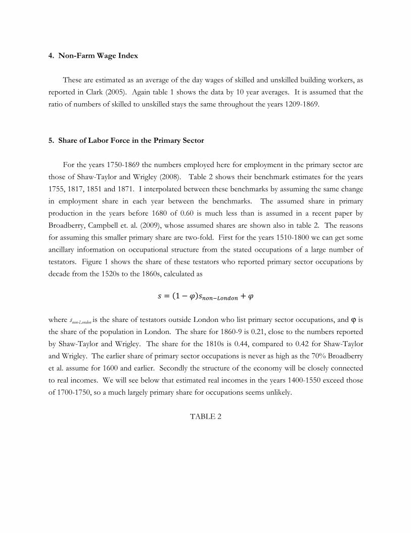
4. Non-Farm Wage Index
These are estimated as an average of the day wages of skilled and unskilled building workers, as
reported in Clark (2005). Again table 1 shows the data by 10 year averages. It is assumed that the
ratio of numbers of skilled to unskilled stays the same throughout the years 1209-1869.
5. Share of Labor Force in the Primary Sector
For the years 1750-1869 the numbers employed here for employment in the primary sector are
those of Shaw-Taylor and Wrigley (2008). Table 2 shows their benchmark estimates for the years
1755, 1817, 1851 and 1871. I interpolated between these benchmarks by assuming the same change
in employment share in each year between the benchmarks. The assumed share in primary
production in the years before 1680 of 0.60 is much less than is assumed in a recent paper by
Broadberry, Campbell et. al. (2009), whose assumed shares are shown also in table 2. The reasons
for assuming this smaller primary share are two-fold. First for the years 1510-1800 we can get some
ancillary information on occupational structure from the stated occupations of a large number of
testators. Figure 1 shows the share of these testators who reported primary sector occupations by
decade from the 1520s to the 1860s, calculated as
1
where snon-London is the share of testators outside London who list primary sector occupations, and ϕ is
the share of the population in London. The share for 1860-9 is 0.21, close to the numbers reported
by Shaw-Taylor and Wrigley. The share for the 1810s is 0.44, compared to 0.42 for Shaw-Taylor
and Wrigley. The earlier share of primary sector occupations is never as high as the 70% Broadberry
et al. assume for 1600 and earlier. Secondly the structure of the economy will be closely connected
to real incomes. We will see below that estimated real incomes in the years 1400-1550 exceed those
of 1700-1750, so a much largely primary share for occupations seems unlikely.
TABLE 2
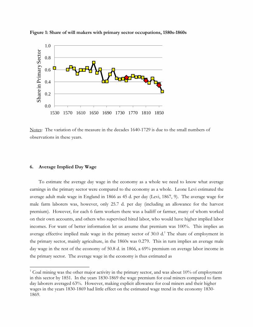
Figure 1: Share of will makers with primary sector occupations, 1580s-1860s
Notes: The variation of the measure in the decades 1640-1729 is due to the small numbers of
observations in these years.
6. Average Implied Day Wage
To estimate the average day wage in the economy as a whole we need to know what average
earnings in the primary sector were compared to the economy as a whole. Leone Levi estimated the
average adult male wage in England in 1866 as 45 d. per day (Levi, 1867, 9). The average wage for
male farm laborers was, however, only 25.7 d. per day (including an allowance for the harvest
premium). However, for each 6 farm workers there was a bailiff or farmer, many of whom worked
on their own accounts, and others who supervised hired labor, who would have higher implied labor
incomes. For want of better information let us assume that premium was 100%. This implies an
average effective implied male wage in the primary sector of 30.0 d.1 The share of employment in
the primary sector, mainly agriculture, in the 1860s was 0.279. This in turn implies an average male
day wage in the rest of the economy of 50.8 d. in 1866, a 69% premium on average labor income in
the primary sector. The average wage in the economy is thus estimated as
1 Coal mining was the other major activity in the primary sector, and was about 10% of employment in this sector by 1851. In the years 1830-1869 the wage premium for coal miners compared to farm day laborers averaged 63%. However, making explicit allowance for coal miners and their higher wages in the years 1830-1869 had little effect on the estimated wage trend in the economy 1830-1869.
0.0
0.2
0.4
0.6
0.8
1.0
1530 1570 1610 1650 1690 1730 1770 1810 1850
Shar
e in
Prim
ary S
ecto
r
W = bω σ Wa + (1-b) σ(Wc + Wl)
where b is the share of labor employed in primary occupations, Wa the farm laborer wage, Wc the
wage of building craftsmen, Wl the wage of building laborers, and adjustment factors of ω = 1.169,
σ = 0.582, to set the correct average wage levels in each sector. This wage is shown by decade in
table 1.
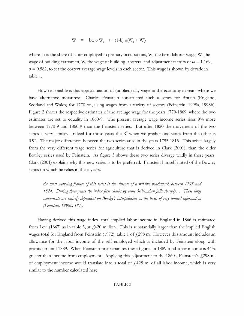
How reasonable is this approximation of (implied) day wage in the economy in years where we
have alternative measures? Charles Feinstein constructed such a series for Britain (England,
Scotland and Wales) for 1770 on, using wages from a variety of sectors (Feinstein, 1998a, 1998b).
Figure 2 shows the respective estimates of the average wage for the years 1770-1869, where the two
estimates are set to equality in 1860-9. The present average wage income series rises 9% more
between 1770-9 and 1860-9 than the Feinstein series. But after 1820 the movement of the two
series is very similar. Indeed for those years the R2 when we predict one series from the other is
0.92. The major differences between the two series arise in the years 1795-1815. This arises largely
from the very different wage series for agriculture that is derived in Clark (2001), than the older
Bowley series used by Feinstein. As figure 3 shows these two series diverge wildly in these years.
Clark (2001) explains why this new series is to be preferred. Feinstein himself noted of the Bowley
series on which he relies in these years.
the most worrying feature of this series is the absence of a reliable benchmark between 1795 and
1824. During these years the index first climbs by some 56%...then falls sharply… These large
movements are entirely dependent on Bowley’s interpolation on the basis of very limited information
(Feinstein, 1998b, 187).
Having derived this wage index, total implied labor income in England in 1866 is estimated
from Levi (1867) as in table 3, at £420 million. This is substantially larger than the implied English
wages total for England from Feinstein (1972), table 1 of £298 m. However this amount includes an
allowance for the labor income of the self employed which is included by Feinstein along with
profits up until 1889. When Feinstein first separates these figures in 1889 total labor income is 44%
greater than income from employment. Applying this adjustment to the 1860s, Feinstein’s £298 m.
of employment income would translate into a total of £428 m. of all labor income, which is very
similar to the number calculated here.
TABLE 3
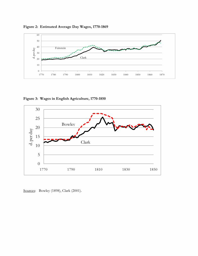
Figure 2: Estimated Average Day Wages, 1770-1869
Figure 3: Wages in English Agriculture, 1770-1850
Sources: Bowley (1898), Clark (2001).
0
10
20
30
40
50
60
1770 1780 1790 1800 1810 1820 1830 1840 1850 1860 1870
d. p
er d
ay
Clark
Feinstein
0
5
10
15
20
25
30
1770 1790 1810 1830 1850
d. p
er d
ay
Clark
Bowley
7. Skill Premium
The last column of table 1 shows the skill premium, which is measured here by the relative
wage of skilled building workers compared to building laborers.
8. Population and labor supply
The population before 1540 is estimated as in Clark (2007a). Since this gives decadal estimates
the other years are interpolated geometrically, except in the periods 1310-19 and 1340-49 where the
timing of the shocks to population in those decades is known. Thus population is assumed to have
fallen to the 1320s level by 1318, and to the 1350s level by 1349. The population after 1540 is
estimated from Wrigley et al. (1997, 614) to 1805. Thereafter the census totals for England
including Monmouth are used, interpolating between the census dates. These estimates by decade
are shown as the last column in table 1.
These population numbers for the years before 1500 are controversial. Whereas these estimates
imply a population for England c. 1300 of 5.3 million, Bruce Campbell has argued for a much lower
population of only 4.25 million. Table 4 shows the population assumed here versus that of
Broadberry, Campbell et al. As can be seen for the years 1520 and earlier the estimates here are of a
consistently higher population by a margin of 17-30%. Clark (2007b) explains and defends these
population estimates.
TABLE 4
9. Days Worked per Year
This is a very difficult issue. There is widespread belief that the numbers of days per year
worked by the population increased greatly between 1200 and 1800, but surprisingly little direct
evidence of any substantial increase in work days over this interval (Clark and Van der Werf, 1998;
de Vries, 1994, 2008; Voth, 2001a, 2001b). Despite the lack of direct evidence of much change in
days worked per year Broadberry, Campbell et al. assume widely varying days worked per farm
family over the years 1250-1850, as is shown in table 5. They assume an “industrious revolution” in
the years 1700-1850, with a one third increase in days worked per farm family. But they also assume
a “de-industrious revolution” in the years 1300-1450, when work days are assumed to decline by
nearly 30%. Thus assumed work days per year per farm family are double in 1850 what they are in
1450. The reason they make the assumptions about work days per year is in order to reconcile their
estimates of farm outputs directly with estimates of farm output from factor payments (wages, land
rents, etc.). Farm wages are so high in 1450, for example, that the total farm output implied if all
workers were fully employed would greatly exceed the directly estimated output. This mismatch,
however, in part stems from the very high assumed farm share of employment that the authors
adopt for the years before 1700.
TABLE 5
If there was a rise in work hours per person in England in the years 1650-1800, we would think
that it would be possible to demonstrate it in data from the labor market. However, the evidence
here for England, even for male workers, the easiest to observe, is at best ambiguous. At worst it
suggests no significant increase in work hours for adult males between even 1250 and 1800.
Clark and van der Werf (1998), for example, find evidence for only a very modest rise in days
worked per year by men in the years 1560-1860. If workers were employed by the year and by the
day, the days per year of the annual workers should be,
days per year = annual wage/day wage.
Complicating factors, such as that yearly workers have more security and might thus accept a lower
daily wage, will affect the exact ratio here. Or again annual workers may be better workers and so
get a higher daily wage.2 But as long as the selection process is the same over time we can use these
payment ratios to look at relative days worked per year over time. Table 6 shows this calculation of
the typical number of days in the work year as the ratio between the annual payment of workers
compared to the day wage of similar workers. Since the table is based on small samples of workers
paid in both ways, the standard error of the error is also estimated. The true number of work days
will lie within two times the standard error of the estimate given 95 percent of the time.
TABLE 6
The implied work year for farm workers in the 1870s was 280-311. Back in 1560-99 it was only 257.
So the best estimate is of a 10-15 percent increase in work days over this interval. This exercise
suggests at best modest increases in days per year between 1560 and 1800. Other measures of likely
2. Alternately, employers may pay less per day for annual workers than for day workers because they then have commitments to use workers for a longer period.
days per year suggest there may have been no increase. We can, for example, calculate at least the
common language interpretation of the number of work days in a week in a similar way to days per
year. This is by looking at the ratio of the weekly wages quoted for building workers to their daily
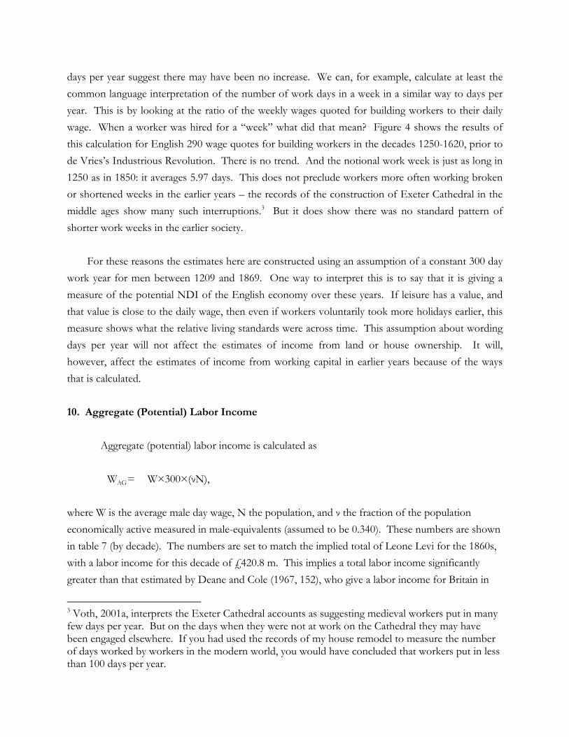
wage. When a worker was hired for a “week” what did that mean? Figure 4 shows the results of
this calculation for English 290 wage quotes for building workers in the decades 1250-1620, prior to
de Vries’s Industrious Revolution. There is no trend. And the notional work week is just as long in
1250 as in 1850: it averages 5.97 days. This does not preclude workers more often working broken
or shortened weeks in the earlier years – the records of the construction of Exeter Cathedral in the
middle ages show many such interruptions.3 But it does show there was no standard pattern of
shorter work weeks in the earlier society.
For these reasons the estimates here are constructed using an assumption of a constant 300 day
work year for men between 1209 and 1869. One way to interpret this is to say that it is giving a
measure of the potential NDI of the English economy over these years. If leisure has a value, and
that value is close to the daily wage, then even if workers voluntarily took more holidays earlier, this
measure shows what the relative living standards were across time. This assumption about wording
days per year will not affect the estimates of income from land or house ownership. It will,
however, affect the estimates of income from working capital in earlier years because of the ways
that is calculated.
10. Aggregate (Potential) Labor Income
Aggregate (potential) labor income is calculated as
WAG = W×300×(νN),
where W is the average male day wage, N the population, and ν the fraction of the population
economically active measured in male-equivalents (assumed to be 0.340). These numbers are shown
in table 7 (by decade). The numbers are set to match the implied total of Leone Levi for the 1860s,
with a labor income for this decade of £420.8 m. This implies a total labor income significantly
greater than that estimated by Deane and Cole (1967, 152), who give a labor income for Britain in
3 Voth, 2001a, interprets the Exeter Cathedral accounts as suggesting medieval workers put in many few days per year. But on the days when they were not at work on the Cathedral they may have been engaged elsewhere. If you had used the records of my house remodel to measure the number of days worked by workers in the modern world, you would have concluded that workers put in less than 100 days per year.
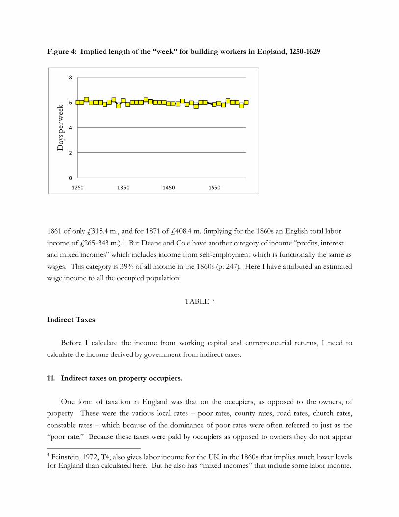
Figure 4: Implied length of the “week” for building workers in England, 1250-1629
1861 of only £315.4 m., and for 1871 of £408.4 m. (implying for the 1860s an English total labor
income of £265-343 m.).4 But Deane and Cole have another category of income “profits, interest
and mixed incomes” which includes income from self-employment which is functionally the same as
wages. This category is 39% of all income in the 1860s (p. 247). Here I have attributed an estimated
wage income to all the occupied population.
TABLE 7 Indirect Taxes
Before I calculate the income from working capital and entrepreneurial returns, I need to
calculate the income derived by government from indirect taxes.
11. Indirect taxes on property occupiers.
One form of taxation in England was that on the occupiers, as opposed to the owners, of
property. These were the various local rates – poor rates, county rates, road rates, church rates,
constable rates – which because of the dominance of poor rates were often referred to just as the
“poor rate.” Because these taxes were paid by occupiers as opposed to owners they do not appear
4 Feinstein, 1972, T4, also gives labor income for the UK in the 1860s that implies much lower levels for England than calculated here. But he also has “mixed incomes” that include some labor income.
0
2
4
6
8
1250 1350 1450 1550
Day
s per
wee
k
above under land rent and tithes, though their incidence probably lay mainly on the rental value of
land and houses.
There are totals of such rates for England and Wales in the years 1747-9, 1775, 1782-4, 1802,
1812-69 (Mitchell, 1962, 410-11). These are converted to an English basis by multiplying by the
share of the population English in 1801 (0.94). To estimate poor rate payments in other years data
was collected from the parish accounts of 33 parishes in Bedford, Dorset, Essex, Warwick, over the
years 1577-1869. Payments in each parish relative to the years 1824-33 were calculated for each year
with data. An average (weighted by the size of payments 1824-33) was then calculated for each year.
Payments on this index are shown by ten year averages in table 7. Before 1600 the amounts of these
taxes was modest, and they are assumed 0 for the years before 1570 when there are no records of
their size.
Later I also need to calculate what share of these taxes was paid from farmland. In 1832 poor
rates per head were about double in parishes with all the employment in agriculture than they were
in parishes where none of the employment was agricultural. I thus assume throughout all these
years that this differential was the same. Then I calculate the share of poor rates paid by the farming
sector as 21
where θ is the share of the population employed in farming. This would imply that if θ = 0.5, the
share paid by the farming sector would be 0.67.
12. Commodity Taxes
In the eighteenth century indirect taxes on commodities became an important source of
government income in England. Under the pressures of war finance demands the government
introduced significant taxation of many commodities – beer, wine, candles, bricks, paper, etc. The
revenue from these indirect taxes – customs dues, excise taxes – is reported for the UK 1801-1869,
for Great Britain1689-1800 and 1807-1816, for England and Wales, 1660-1688 (Mitchell, 1962, 386-
8, 392-3). UK figures are reduced to those for Great Britain by multiplying by 0.92 their relative
share in 1807-16. Totals for Great Britain are reduced to those for England alone by multiplying
them by 0.84, based on the population of England relative to Great Britain in 1801. Before 1551
indirect taxes are taken as 0% of national income, since in the years 1551-57 they averaged only
0.2% of national income. Table 7 shows decadal totals for indirect taxes.

Property Income
To get the total gross value of income in the economy we need to add to wage income the
returns from ownership of property: land, houses, shops, industrial buildings, roads, canals,
waterways, mines, machines, and working capital such as farm animals and horses. After 1842 we
have information on such returns from the Property and Income Tax Returns. These returns
distinguish income from property of the following types: lands, houses, tithes, manors, fines,
quarries, mines, iron works, fisheries, canals, and railways. For the 1860s the average of these
reported incomes, reduced to the basis of England, was as follows:
Farmland and farm buildings (including tithe) £46.0 m.
Other houses and buildings £60.3 m.
Profits from land occupation £23.0 m.5
Profits of Mines, Canals, Railways, etc. £21.0 m.
Other business and professional incomes £84.4 m.6
The tax returns thus do not give any real estimate of property income in agriculture. Also
business and professional incomes exclude some incomes under £100 which were earlier exempt
from tax, and this exemption limit was lifted to £150 in 1853. For those with incomes of £100 or
less in business or a profession the majority would likely actually be wage income (in the 1860s the
annual earnings of a building craftsman would be £66). Thus the tax reports of business and
professional incomes includes wage income for small proprietors and professionals. Here I take as
property income all business and professional income of £150 or greater 1842-1869. It is assumed
here that the exclusions of the property incomes with those with gross incomes under £150 cancel
out the inclusion of wage income for those with income of £150 or more. The proportions of each
class in 1855-6 in England among reported incomes were
Less than £100 £5.9 m
£100-£150 £10.6 m
More than £150 £49.4 m7
5 This was assessed as ½ of land rental values (Stamp, 1922, 82). 6 Counting only such incomes £150 or greater. See below. 7 Stamp, 1922, 511.

But there is reason to believe that there may be underreporting of the “less than £100” income
group who were not liable for the income tax.
The tax returns report the gross income from farmland and housing and other buildings. For
business incomes the 1842 Tax Acts allowed deductions for sums expended in “for the repairs of
premises and the supply or repair of alterations of any implements” (Stamp, 1922, 178). Thus
business and professional income was effectively assessed as net income.
13. Farmland Rental Income
Land rents are estimated from the market rental values, including tithes and land taxes that fell
on occupiers, of plots of unchanging area over the years 1209-1869. The rent paid to the owner of
land was only one claim on the site value of the land. In addition there was the tithe due originally
to the church, but later to private owners of tithe rights. This was nominally 10 percent of the gross
output of the land but was later collected at typically much lower rates. Also increasingly from 1600
on there were local parish levies to support the poor, and pay for the roads and other services. By
the nineteenth century were 6-10 percent of the rents paid by occupiers.
The rent series used here gives the rental value of farmland inclusive of the tithe, but not
including taxes paid by occupiers which are enumerated separately. The details of how this was
constructed for the later years are discussed in Clark (2002a). This series thus includes imputed
rents in the case where owners were also occupiers. Much land was bundled with dwellings, and the
land rents measured here thus include payments for farmhouses and farm buildings.
To avoid problems of land quality and varying land measures the series is constructed by
looking at what happens to the same plot over time, except in the medieval period where the less
rigorous measure of the same type of land in the same village is used. The rent series thus
incorporates and values in earlier years communal “waste” land only later brought into private
cultivation. It is assumed throughout that there were 28.24 m. acres of farmland in England, though
in earlier years some of this would be uncultivated waste. From 1842 on these rental values are
estimated from Income and Property tax returns (Stamp, 1922, 49). Tables 7 and A2 shows the
value for England of these imputed land rents.
It is also assumed that land rents represented rents net of repairs to fences, ditches and
buildings, which are assumed to be made by the tenants.
14. Returns to capital
For England evidence on interest rates goes back to about 1170. Figure 5 shows the rate of
return on two very low risk investments in England from 1170 to 1900. The first is the gross return
on investments in agricultural land, R/P, where R is the rental and P the price of land. This can
differ from the real return on land,
)( ππ −+= LP
Rr
where πL is the rate of increase of land prices and π is the general rate of inflation. (πL - π) is the
rate of increase of real land values. But the rate of increase in real land values in the long run has to
be low in all societies, and certainly was low in pre-industrial England. If the rate of increase of real
land prices was as high as 1% per year from 1300 to 1800, for example, it would increase the real
value of land by 144 times over this period. Thus the rent/price ratio of land will generally give a
good approximation to the real interest rate in the long run.
The second rate of return is that for “rent charges.” Rent charges were perpetual fixed nominal
obligations secured by land or houses. The ratio of the sum paid per year to the price of such a rent
charge gives the interest rate for another very low risk asset, since the charge was typically much less
than the rental value of the land or house. The major risk in buying a rent charge would be that
since it is an obligation fixed in nominal terms, if there is inflation the buyer gets a lower real rate of
return. Again the gross rate of return shown is R/P, where R = annual payment, P = price of rent
charge. The real rate of return, r, in this case is
π−=P
Rr
Table 8 shows the assumed risk-free return on capital by decade 1200-1869, taken as the
average of these two rates.
TABLE 8
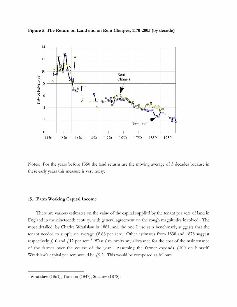
Figure 5: The Return on Land and on Rent Charges, 1170-2003 (by decade)
Notes: For the years before 1350 the land returns are the moving average of 3 decades because in
these early years this measure is very noisy.
15. Farm Working Capital Income
There are various estimates on the value of the capital supplied by the tenant per acre of land in
England in the nineteenth century, with general agreement on the rough magnitudes involved. The
most detailed, by Charles Wratislaw in 1861, and the one I use as a benchmark, suggests that the
tenant needed to supply on average £8.68 per acre. Other estimates from 1838 and 1878 suggest
respectively £10 and £12 per acre.8 Wratislaw omits any allowance for the cost of the maintenance
of the farmer over the course of the year. Assuming the farmer expends £100 on himself,
Wratislaw’s capital per acre would be £9.2. This would be composed as follows
8 Wratislaw (1861), Tomson (1847), Squarey (1878).
Live Stock 60%
Implements 11%
Seed, Labor, Horse and Cattle Food 21%
Rent, tithe and taxes in advance 3%
Maintenance of farmer 5%
Allowing the farmer just the return on capital from bonds or mortgages, this would imply a
capital cost in the 1860s of £0.39 per acre. However, as with all business enterprises their has to be
an additional return based on the risk of the enterprise. Farming was not a high return activity so I
set this additional return at 3%. This raises the working capital return per acre to £0.69. The land
rent actually includes a substantial amount that is a return to capital in the form of buildings and
land improvement. Conventionally the farmers profit was expected to be half the rental of the land
before 1896 (Stamp, 1922, 82), though this return included the farmer’s wage which I have included
elsewhere. With a land rental in the 1860s of £46 m, that would imply a profit income of £23 m.
The net profit income on working capital calculated here for the 1860s is £19 m.
To estimate the equivalent capital costs for the other decades I make the following
assumptions. First that the interest cost of the capital employed by farmers was the average of the
return on rent charges and land, plus 3% for risk. Second that the price of capital goods was the
same as the price of farm output. Since live stock, seeds, and animal food were the majority of the
capital stock, and implements were a small share, this assumption seems reasonably innocuous.
Lastly I assume that the capital-output ratio for the farmer’s capital did not change over time. This
last assumption is the most contentious. But again when we consider the importance of animals,
fodder and seeds in farmer’s capital it does not seem that there was any reason to expect any change
in the capital output ratio over time. With these assumptions I get the implied payments for
working capital in agriculture shown in table 8.
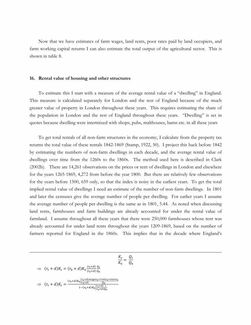
In table 8 the payments to capital in year t are calculated, using these assumptions, as 1
where r0 = return on capital in the 1860s, r1 = return on capital in year t.9
9 This follows from the fact that, by assumption
Now that we have estimates of farm wages, land rents, poor rates paid by land occupiers, and
farm working capital returns I can also estimate the total output of the agricultural sector. This is
shown in table 8.
16. Rental value of housing and other structures
To estimate this I start with a measure of the average rental value of a “dwelling” in England.
This measure is calculated separately for London and the rest of England because of the much
greater value of property in London throughout these years. This requires estimating the share of
the population in London and the rest of England throughout these years. “Dwelling” is set in
quotes because dwelling were intermixed with shops, pubs, malthouses, barns etc. in all these years
To get total rentals of all non-farm structures in the economy, I calculate from the property tax
returns the total value of these rentals 1842-1869 (Stamp, 1922, 50). I project this back before 1842
by estimating the numbers of non-farm dwellings in each decade, and the average rental value of
dwellings over time from the 1260s to the 1860s. The method used here is described in Clark
(2002b). There are 14,261 observations on the prices or rent of dwellings in London and elsewhere
for the years 1265-1869, 4,272 from before the year 1800. But there are relatively few observations
for the years before 1500, 659 only, so that the index is noisy in the earliest years. To get the total
implied rental value of dwellings I need an estimate of the number of non-farm dwellings. In 1801
and later the censuses give the average number of people per dwelling. For earlier years I assume
the average number of people per dwelling is the same as in 1801, 5.44. As noted when discussing
land rents, farmhouses and farm buildings are already accounted for under the rental value of
farmland. I assume throughout all these years that there were 250,000 farmhouses whose rent was
already accounted for under land rents throughout the years 1209-1869, based on the number of
farmers reported for England in the 1860s. This implies that in the decade where England’s
population was estimated to be at its lowest, the 1440s with only 2.27 million people, aside from an
assumed 250,000 farmhouses there were only 168,000 other dwellings.
The implied rental income reported here is a gross rental. Thus to get the net rental income we
need to deduct repairs. Clark (1998a) calculates the return on land and housing in England by
quinquennia for the eighteenth and nineteenth centuries. The returns on housing average about 2%
more than those on land, suggesting that the depreciation rate for housing is about 2%. To get the
net rental of housing I deduct for each period a fraction of the estimated rental which is:
2 2
where r is the return on land (in percent). The total net rental is shown in table 8 also.
17. Other Property Incomes
The Property Tax returns for the years 1842 and later distinguish property incomes from
quarries, coal mines, canals, railways and iron works (Stamp, 1922, 220). These reported sums are
for Great Britain for the years 1842-1853, and the UK thereafter. To convert them to an English
basis I assume, unless otherwise indicated, that England was 84% of British economic activity and
that after 1853 there was no income in Ireland from quarries, coal mines, ironworks, canals, railways
and gasworks (there would be some income but it assumed to be negligibly small). These returns do
not include, however, the imputed income from capital invested in roadways. These property
incomes are in each case carried back to 1730. In addition I estimate the property income from ship
ownership from 1730 to 1869.
Coal Mining and Quarrying
For 1842-69 I calculate the share of coal production from England from the share 1854-69
given in Mitchell (1962, 115). For 1842-53 that is taken as 75%, the same share as 1854-5. I assume
quarries had the same output distribution as coal mines.
To estimate returns from coal mines earlier than 1842 I use Clark and Jacks (2007), which
estimates by decade from the 1730s on coal output, pithead prices, coal ground rents, and the share
of capital returns in output prices, which through the 1730s-1860s averaged 20%. Table 9 shows
these estimates. Coal mineral rents are calculated directly by decade. Capital returns are calculated
as 20% of the total production cost throughout, based on estimates from colliery accounts in the
years 1720-1860. All property income, the last column includes a 12% addition to account for
quarries as well as coal mines, based on the post 1842 tax returns (Stamp, 1924, 220).
TABLE 9
Railways
Table 10 shows the estimated property income from railways in the 1840s to 1860s from the
Property Tax returns. This income before 1853 is given for Britain, and is reduced to an English
basis by multiplying by 0.84 (Stamp, 1924, 220). After 1853 the report is for the entire UK. The
share attributed to Britain is calculated using the relative paid up capital of British and Irish railways
(Mitchell, 1962, 225-228), and is then reduced to an English basis by being multiplied by 0.84.
Before 1842 property income from railways is estimated on the basis of the miles of line completed
in the UK relative to 1842 (Mitchell, 1962, 225), multiplied by the same property earnings as in 1842.
TABLE 10
Canals
Canal and improved river mileage in England from 1750 to 1850 is from Ginarlis and Pollard
(1988), table 8.7, 213-215. For 1730-49 I assume the same mileage as in 1750. Property income per
canal or waterway mile is assumed to be equal to that of the 1840s, but converted into current terms
by the cost of a day of farm labor. These returns are shown also in table 10.
Iron Works
To estimate the profit earnings from iron works 1842-1869 I assume no iron was produced in
Ireland, and the earnings in England were the total British earnings multiplied by the share of pig
iron produced in England in 1842-1869 (Mitchell, 1962, 131). To project this back as far as the
1720s I use estimates of the tons of English pig iron output per year at benchmark dates (Mitchell,
1962, 131), multiplied by the price of manufactured iron to get an estimate of the value of output
earlier. It is assumed capital returns are the same fraction of the value of output in the 1842 as in
each earlier decade. These returns are also shown by decade in table 10.
Roads
Another form of capital was the road system. This generally did not produce an explicit rental
income, except where roads were turnpiked and maintained from toll revenue, mainly in the period
1750-1840. In other periods roads were paid for by levies on parish occupants, or by local and
county rates on property. The rate payments are calculated below. In earlier years when there were
direct labor levies for work on the parish roads these will be counted in the calculated labor income
in the economy. But if we want to count all sources of income then we need to include the implicit
turnpike property income, from the capital invested in turnpike roads and paid for through toll
collections, for the years 1696-1869.
To do this I first calculate (roughly) the average miles of turnpike road in England in each
decade (Pawson, 1977, 155-6; Bogart, 2005, 440). I calculate the average capital invested in a
turnpike road from Bogart, 2005, 454: this shows road expenditure per mile in 1819 prices for the 10
years after establishing a new turnpike. The investment in the first year is £260, the second £170,
the third £100, fourth £90 and fifth £80. But thereafter there is a steady state expenditure of £75
per year. I presume the new investment is all of the first year investment, plus all sums thereafter
above the presumed maintenance cost of £75 per mile. This gives £400 per mile. I convert this
cost into the prices of each decade using the level of farm wages (since labor was the major
component of this investment). I assume that the return on this capital throughout these years was
5%. These estimates are shown in table 11.
TABLE 11
Ships
The volume of shipping services used by the economy expanded dramatically in the Industrial
Revolution era, as England became dependent on imported food and raw materials, and as the cities
relied on coal from the northern coal fields as their primary energy source. There are statistics on
the net tonnage of ships registered in the UK, 1788-1869 (Mitchell, 1962, 217-8). Mostly sailing
ships even up to 1869 (when 83% still sailing tonnage). To get an estimate of what fraction of these
ships were operating from English ports I rely on the data in Davis (1956) on the numbers of sailors
paying the “sailor’s sixpence” tax in England and the UK between 1707 and 1828. This allows me
to divide up the tonnage from 1788 and later between England and the rest of the UK (the English
share is typically 85-90% of the UK share). For the years 1707-1787 I estimate the English tonnage
from the number of sailors alone assuming it had the same ratio to sailors as in 1788-1897. This
gives the data reported in column 2 of table 12 on the total tonnage of English shipping. Estimating
the value of that tonnage is difficult. There are various piecemeal estimates of the cost of a ship,
fully rigged and outfitted, for the years 1670-1858.10 These give a rough estimate of the cost of a
new ship for various benchmark dates, which I interpolate using a very rough cost index (with a .67
weight for wages, and .33 for timber). The overall cost index moves in line with the input price
index. I assume in calculating the value of the shipping stock that the average working ship had a
value 2/3 that of a new ship (there were substantial losses of ships each year from accidents and loss
in war). Feinstein, 1988, 439, gives decadal estimates of the net stock of ships in Great Britain from
1760 to 1850, and from 1851-1869 annual estimates of the UK ship stock, though it is not indicated
where the figures for the years before 1851 come. The implied value of the English shipping stock
on his measures are also shown in table 12. His numbers are much smaller, one reason being that he
assumes the value of the net stock is about half that of the gross stock.
TABLE 12
Davis (1957) and others have investigated the return on ship ownership. Davis conclusion is
that ships earned a net return substantially in excess of the risk free return on capital, because of
considerable uncertainties on the profitability of voyages because of the hazards of captains, trade,
warm, and the weather. Losses of shipping could be insured against, but not losses of income from
the failures of ventures. I thus assume that the profit rate on this capital was 5% beyond that of the
return on land or rent changes. This is in line with the estimate of Barney (1999, 137) that the
King’s Lynn firm of W. & T. Bragge earned an average net profit of 9% in the 30 years 1766-1795.
Column 6 of table 12 shows the implied rental on ships from the 1700s to the 1860s. The final
column of table 12 shows the sum of all the non-structure capital incomes – coal mines, quarries,
railways, canals, roads, ironworks, gasworks, and ships.
10 Davis, 1957, 410 estimates the cost 1670-1730 at £11 per ton (£6.5 for the hull and masts, £4.5 for the rigging), Barney, 1999, 132 quotes ship prices per ton of £9.7 in the 1760s, and £10.5 1783-90. Ville, 1990, 47-51 gives ship prices in the coal trade 1792-1825. Harley, 1988, 872 quotes prices for 1833 and 1852-8. Graham, 1956, 80, gives prices for 1825 and 1847.
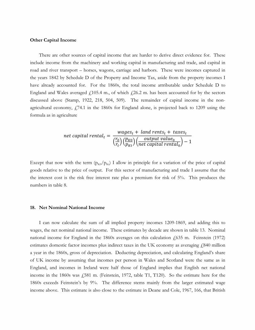
Other Capital Income
There are other sources of capital income that are harder to derive direct evidence for. These
include income from the machinery and working capital in manufacturing and trade, and capital in
road and river transport – horses, wagons, carriage and harbors. These were incomes captured in
the years 1842 by Schedule D of the Property and Income Tax, aside from the property incomes I
have already accounted for. For the 1860s, the total income attributable under Schedule D to
England and Wales averaged £105.4 m., of which £26.2 m. has been accounted for by the sectors
discussed above (Stamp, 1922, 218, 504, 509). The remainder of capital income in the non-
agricultural economy, £74.1 in the 1860s for England alone, is projected back to 1209 using the
formula as in agriculture
1
Except that now with the term (pK0/pKt) I allow in principle for a variation of the price of capital
goods relative to the price of output. For this sector of manufacturing and trade I assume that the
the interest cost is the risk free interest rate plus a premium for risk of 5%. This produces the
numbers in table 8.
18. Net Nominal National Income
I can now calculate the sum of all implied property incomes 1209-1869, and adding this to
wages, the net nominal national income. These estimates by decade are shown in table 13. Nominal
national income for England in the 1860s averages on this calculation £635 m. Feinstein (1972)
estimates domestic factor incomes plus indirect taxes in the UK economy as averaging £840 million
a year in the 1860s, gross of depreciation. Deducting depreciation, and calculating England’s share
of UK income by assuming that incomes per person in Wales and Scotland were the same as in
England, and incomes in Ireland were half those of England implies that English net national
income in the 1860s was £581 m. (Feinstein, 1972, table T1, T120). So the estimate here for the
1860s exceeds Feinstein’s by 9%. The difference stems mainly from the larger estimated wage
income above. This estimate is also close to the estimate in Deane and Cole, 1967, 166, that British
domestic income (gross of some capital depreciation) was £648 m. in 1861 and £877 m. in 1871.
This implies an English domestic income in the 1860s of £599 m.
TABLE 13
Table 13 also shows the share of wages, land rents and capital in national income, where that
share of wages is calculated as
.
This calculation suggests the share of wages varied between 48 and 76% of national income,
reaching the highest share, 76%, in the 1860s. The share of land rents is
.
This share before 1800 varied between 15 and 30% of national income, but by the 1860s had fallen
to 9%. The share of capital is calculated as the residual. This method assumes that the burden of
indirect taxes was born equally by labor, land and capital owners.
Table 13 also shows the share of income that comes from the agricultural sector over time.
Since we assumed a certain allocation of labor between farming and the rest of the economy, I can
also estimate the implied relative value of output per worker in agriculture compared to the rest of
the economy. That ratio is shown as the last column of table 13.
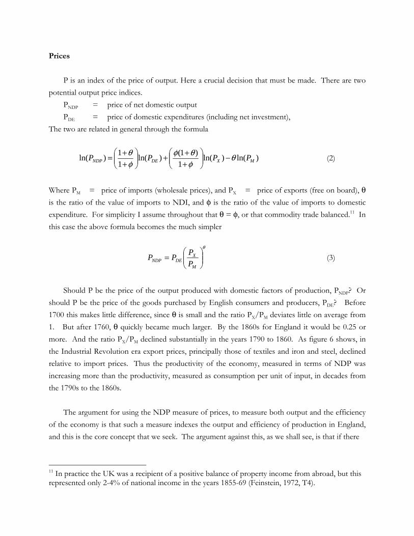
Prices
P is an index of the price of output. Here a crucial decision that must be made. There are two
potential output price indices.
PNDP = price of net domestic output
PDE = price of domestic expenditures (including net investment),
The two are related in general through the formula
)ln()ln(1
)1()ln(11)ln( MXDENDP PPPP θ
φθφ
φθ −
+++
++= (2)
Where PM = price of imports (wholesale prices), and PX = price of exports (free on board), θ
is the ratio of the value of imports to NDI, and φ is the ratio of the value of imports to domestic
expenditure. For simplicity I assume throughout that θ = φ, or that commodity trade balanced.11 In
this case the above formula becomes the much simpler
θ
=
M
XDENDP P
PPP (3)
Should P be the price of the output produced with domestic factors of production, PNDP? Or
should P be the price of the goods purchased by English consumers and producers, PDE? Before
1700 this makes little difference, since θ is small and the ratio PX/PM deviates little on average from
1. But after 1760, θ quickly became much larger. By the 1860s for England it would be 0.25 or
more. And the ratio PX/PM declined substantially in the years 1790 to 1860. As figure 6 shows, in
the Industrial Revolution era export prices, principally those of textiles and iron and steel, declined
relative to import prices. Thus the productivity of the economy, measured in terms of NDP was
increasing more than the productivity, measured as consumption per unit of input, in decades from
the 1790s to the 1860s.
The argument for using the NDP measure of prices, to measure both output and the efficiency
of the economy is that such a measure indexes the output and efficiency of production in England,
and this is the core concept that we seek. The argument against this, as we shall see, is that if there
11 In practice the UK was a recipient of a positive balance of property income from abroad, but this represented only 2-4% of national income in the years 1855-69 (Feinstein, 1972, T4).
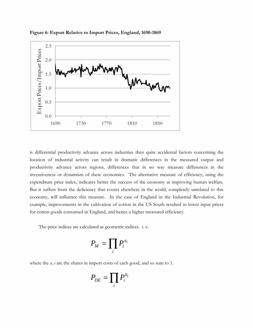
Figure 6: Export Relative to Import Prices, England, 1690-1869
is differential productivity advance across industries then quite accidental factors concerning the
location of industrial activity can result in dramatic differences in the measured output and
productivity advance across regions, differences that in no way measure differences in the
inventiveness or dynamism of these economies. The alternative measure of efficiency, using the
expenditure price index, indicates better the success of the economy at improving human welfare.
But it suffers from the deficiency that events elsewhere in the world, completely unrelated to this
economy, will influence this measure. In the case of England in the Industrial Revolution, for
example, improvements in the cultivation of cotton in the US South resulted in lower input prices
for cotton goods consumed in England, and hence a higher measured efficiency.
The price indices are calculated as geometric indices. i. e.
∏=i
aiM
iPP
where the ai s are the shares in import costs of each good, and so sum to 1.
∏=i
biDE
iPP
0.0
0.5
1.0
1.5
2.0
2.5
1690 1730 1770 1810 1850
Exp
ort P
rices
/Im
port
Pric
es
where the bi s are the shares in domestic purchases of each good, and again sum to 1. With this
specification the GDP price index will be of the form
∏=i
ciNDP
iPP
where 1=i
ic , but the individual weights can be positive or negative. Negative weights will
correspond to imported commodities.
The domestic expenditure price index is formed from 11 principle component indexes, whose
weights for each period are shown in table 14. But each of these component indices in turn is
composed of a weighted average of the price of various commodities. The individual price series
were derived as the estimated parameters on year indicators of regressions of the form
ikt
ttt
kkkit DDTYPEP εφβ ++=)ln(
where DTYPE is a set of indicator variables for each type of a product, where a type was defined by
location, purchaser, characteristics and measuring unit. In this I try and control for variations in the
size of units across sources, and in the quality of the product. This is important because both the
quality of the product and the size of the measures varied across sources, even for very homogenous
commodities in the same place at the same time. In London in 1827, for example, the Clothworkers
Guild paid 20 d. per gallon for milk, Bethlem insane asylum 13 d., and the King’s Household 24 d., a
range in price for a seemingly standard product of nearly 2:1. In earlier years where observations are
missing for some years they were interpolated as an 11 year centered moving average of the years
with prices, where this was possible.
TABLE 14
19. Expenditure Prices
The weights of the subcategories in this price index change over time to reflect two things.
First the changing structure of expenditure as the economy became richer in the years 1820-69
following the Industrial Revolution. Second the decline in the number of available price series as we
move to the earliest years of the thirteenth century.
Food Index
This is the most important of the sub-indices, with a weight of at least .45 in the overall
expenditure index. This index consists of the weighted average of a number of sub-indices: starches,
meat, dairy, fish, fats, drink, sugars, salt and spices. The weights were as in table 15.
TABLE 15
Starches: The component series are wheat bread, barley, oats/oatmeal, peas, potatoes, and rice.
The relative weights of each in the starch index are shown in table 16. Up until 1869 wheat bread
was the single most important item of consumption in the economy, getting a weight of at least 9%
in the domestic expenditures index, and at least 13% in the workers’ cost of living index. However,
rather than use bread prices directly I approximate them based on the prices of wheat, labor (skilled
craftsmen), salt, wood fuel and candles. This is done because there is evidence that government
regulation of the bread market before 1815 must created changes in the quality of bread sold over
time. Bread prices are thus estimated (assuming fixed coefficients) as the weighted average of wheat
prices, craft labor, firewood prices, salt prices and candle prices.
TABLE 16
The available bread prices before 1816 are mainly those for London, but these were regulated
by statute before 1815. The statute stipulated how much flour was to be produced per bushel of
wheat, and how many loaves produced from this flour (Webb and Webb, 1904). It also set the
“allowance” the baker received to turn the flour into bread.
If bread prices measured bread of constant quality over time then they should have a very close
relationship to the price of wheat. This is because wheat was the overwhelming cost in making
bread. A breakdown of the costs of bread baked for the Navy in 1767 suggests that the price of
bread should be nearly proportional to that of wheat, since wheat constituted 92% of the costs of
making bread (Beveridge 1939, p. 542). Robert Allen objects that this cost share for wheat is too
high, leaving out the required managerial and capital returns of the baker (Allen, 2008, ---). But if we
calculate the share of wheat costs in bread from the details of the London assize 1797-1813 then we
still find wheat costs were a full 81% of the price of bread (Parliamentary Papers, 1804, 11-12,
Parliamentary Papers, 1812-13, 3, 12). The other elements of costs in 1797-1804 were labor 4.7%,
fuel 1.8%, yeast 1.6%, salt 1.5%, candles 0.4%, and profits 10%. If bread was of constant quality
then bread prices in other years should be predictable from these costs.
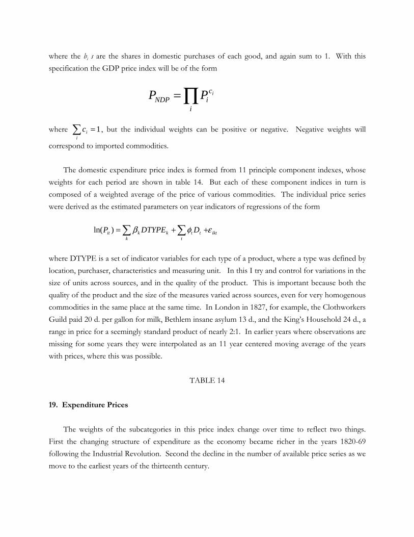
Figure 7 shows the price of bread in London relative to its cost over time: where the cost
elements that I can observe are wheat, labor, fuel, salt and candles. Yeast is assumed to have a cost
proportionate to wheat. And profits are assumed always as 10% of total costs. The figure shows
that the quality of bread cannot be constant over time. After the lifting of the bread assize in 1815
Figure 7: The Bread Price/Cost Ratio,
the price of bread quickly rose nearly 10% relative to the cost. Around 1790 bread sold for about
8% less than its cost of production – so then either bakers were making negative economic profits,
or the quantity of wheat in the standard loaf had been, in effect, reduced.12 Earlier there are other
periods where prices are substantially above costs.13 In this situation it seems much safer to work up
the implied bread price from its component costs than to assume that there were vast swings in the
compensation of bakers, with those of the late 18th century subsidizing their bread sales, and those
of other periods garnering substantial profits.
12 The London assize called for 240 lbs of flour to be made from 6.5 bushels of wheat, or roughly 390 pounds of wheat. The other 150 lbs were lost as bran in the milling process. By milling less finely to produce a coarser flour, more loaves could be made from a bushel of wheat. 13 This does not seem to be a defect of the wheat price series. That series for the years 1771-1869 is very close to the Gazette series, taken from the whole country, of average wheat prices. Yet in this period there is a nearly 20% variation in the price of bread in London relative to wheat prices.
0.9
1
1.1
1.2
1.3
1650 1675 1700 1725 1750 1775 1800 1825 1850
Pri
ce/
Cos
t
Oatmeal prices were used in years where they were available. In other years oatmeal prices were
interpolated using the price of oats.
Meat: The component series are beef, cattle, mutton, sheep, pork, pigs, poulty, and eggs. Meat is
sold by the pound in later years. Earlier to infer meat prices I have to use the prices of live animals.
This will only accurately represent meat prices if animal weights did not change. Since the live
animal series are used in the years 1209-1600, where there is no sign of any yield increases in arable
crops, this seems a reasonable assumption. The weights are given in table 17.
TABLE 17
Dairy: This series is relatively simple, with just milk, butter and cheese, and relatively unchanging
weights throughout. The weights are also shown in table 17.
Fish: The fish series is a weighted average of three components – herring, salt cod, and salt salmon.
The weights are given in table 18.
TABLE 18
Drink: This series incorporates cider, beer, wine, tea and coffee. Here the weights change greatly
over time as is shown in table 19. Over time the favored drinks of the population changed greatly,
in part as a result of substantial changes in the relative prices of the different beverages.
TABLE 19
Sugars: Honey, Currents/Raisins, Sugar, Treacle. Currents and raisins were mainly used as
sweeteners in English cooking. The weights are given in table 20.
TABLE 20
Fuel: The fuel index has three components – wood and peat, charcoal, and coal. Charcoal was a
smokeless version of wood used by the richer. Coal was the smokiest fuel, and hence least desirable.
Because of the high cost of transporting fuel, the use of each was dictated by local supply and
transport conditions. By the eighteenth century coal dominated in big cities like London, but wood
fuel supplies still dominated in countryside locations without good water transport connections.
Table 21 shows the weighs assigned over time to each fuel type.
TABLE 21
Lodging: The method for forming the rental values of housing of constant quality is described in
Clark (2002). For this estimation I have 5,125 observations in total, 757 for the years before 1500.
Over the Industrial Revolution, with greater urbanization, the rental value of housing increased
greatly relative to the general price level. Consequently the weight given to housing in table 14 is
increased in this period. Greater weights are also assigned in the years before 1375 when the return
on capital invested in housing was much greater than in subsequent years, more than 10%, implying
that correspondingly rental values would be greater. Since house rent estimates only go back as far
as the 1290s, for earlier years house rent is estimated as the average of 1290-1349, but indexed by
the relative price level in the earlier year compared to the average price level of 1290-1349.
Light: The component series here are Tallow Candles (in the thirteenth century tallow itself), Wax
Candles, Sperm-Oil, and Coal-Gas. An issue is what weight to give gaslight in this index. After
1815 the price of gas illumination was dramatically below that of candles. It was reckoned that 19
cubic feet of gas had by 1832 the illumination equivalent to a pound of tallow candles (Matthews,
1832, 326). Table 22 shows the cost by decade from 1815-1869 of a pound of tallow candles
compared to the equivalent amount of 19 cubic feet of gas. When gas was being first introduced it
cost only about 40% that of candles. But by the 1850s it cost only about one sixth that of candles.
TABLE 22
It has been argued, however, that before 1870 gas illumination was found only in middle and
upper class homes (Matthews, 1986). However, the poor as well as the rich benefited from the use
of gaslight for street illumination, for pubs, and for shops. By 1876 there were 54,000 street lamps
lit by gas in London alone (Chubb, 1876, 350). It seems thus that the transformation of public
spaces by gas light in the years 1815-1869 should get some weight in the cost of living of even the
poor.
In terms of the weight in the domestic expenditure price index, by the 1860s gas consumption
measured just in the price of gas was about 1% of GNI. In the 1840s it was about 0.5% of GNI
(Matthews, 247). Table 23 shows the weights in the lighting index over time. To allow for the poor
having less access to the benefits of gaslight, in the workers’ cost of living index gas is counted with
only half this national weight. The other weight within the COL light series is all devoted to tallow
candles.
TABLE 23
Clothing and Bedding: The sources for prices here are varied - wool cloth, woolen blankets,
linen cloth, cotton cloth, silk thread, stockings, complete suits of clothing (other than stockings),
boots and shoes, leather gloves. Table 24 shows the weighs assigned over time to each item of
clothing or bedding.
TABLE 24
Services: The pre-industrial economy had a vast array of domestic servants: cooks, housemaids,
grooms, coachmen. This shows even in the 1851 census. At that date, weighting men and women,
boys and girls by their earnings, 13.1% of the labor force was engaged in some type of personal
service (Parliamentary Papers, 1852-3, Table 25, 222-227). Wages were 64% of national income in
1851, so that this implies that 8.4% of expenditure was on service of some kind: domestic servants,
barbers, doctors, nurses, gardeners, and teachers. Thus the share of expenditure devoted to personal
service is assumed at 8% in 1840-69, and somewhat lower in the earlier years (table 14).
Manufactures: Certainly by the end of our period, 1869, the average person was consuming a
quantity of manufactured goods aside from clothing and bedding. There were wooden utensils,
furniture, brooms, hairbrushes, glasswares, cutlery, pottery, pewter, cooking implements, garden
tools, haberdashery, and spectacles. An estimate of the potentially substantial share of these goods
in expenditure comes from insurance policies from the years 1750-1850 analyzed by Sidney Pollard
(Pollard, 1988). The policy value of the average house insured 1801-1850 was £449. At the same
time the value of the contents insured averaged £242, more than half the structure value (Pollard,
1988, 250, 256). The contents consisted of clothing, bedding, plate, jewellery, housewares and
furniture. Unfortunately Pollard does not subdivide this category. But if even just half the value of
housewares was for items other than clothing and bedding, then annual purchases of housewares
and furniture must have been substantial in nineteenth century England.
Using primarily the copious records of the Founding Hospital in London from 1759-1856 I am
able to derives price series for many of these items in the Industrial Revolution period, which I class
under “manufactures.” As table 14 shows these are given a very modest weight in the overall
expenditure index, but were included as a potential area of significant declines in relative prices as a
consequence of the Industrial Revolution.
Investment Goods: Under this heading are included construction materials (bricks, timber,
manufactured iron), as well as implement prices (spades and shovels), and window glass.
Appendix table 1A shows the decadal level of each of the individual price series and the resulting 11
major component price indices.
20. Export Price Index
Table 25 gives total calculated exports and imports from England from 1784-1856 taken from
Davis (1979), and the implied average share of exports and imports of Net National Income. The
total value of English exports is inferred from UK exports for 1834-6 and later, from British exports
for 1784-6 to 1824-6. This is done by assuming that England was 84% of British exports, and that
Ireland received the same share of British exports in later years as in 1824-6. It was assumed
throughout that all cotton goods, wool cloth, manufactures, iron, coal and sugar exports from the
UK were from Britain, with England supplying 84 percent of each. All linen exports from the UK
were assumed to come from Ireland. Table 24 also lists for the major exports that I have price
series their shares of total English exports on these assumptions. The price index for exports was
based on a weighted average of these prices, with the weights changing each 10 years.
TABLE 25
Table 26 shows the total value of exports and imports for England for 1699-1774, where the
export and import data comes from Davis (1962), and refers to England. Table 26 also shows the
share of exports for the commodities for which I have prices over these years.
TABLE 26
The price index for exports was thus composed of indices with the indicated weights for cotton
cloth, woolen cloth, manufactured iron, pig iron, manufactures, coal, sugar and wheat. These should
be FOB prices, but I use as the nearest approximation domestic retail prices.
21. Import Price Index
The main imports of England at various periods are also listed in Tables 25 and 26, taken also
from Davis (1962, 1979). The total value of English imports is inferred from UK imports for 1834-
6 and later, from British imports for 1784-6 to 1824-6, and from English imports for 1699-1701 to
1772-4. This is done by assuming that England was 84% of British imports. For Ireland after 1824-
6 I assume that Irish exports to England were the same in nominal terms in 1834-6, 1844-6, and
1854-6 as in 1824-6. I also assume that Ireland took an amount of the imports of foods to the UK
as equaled its exports to England in these years. For each good after deducting the assumed share
of Ireland I assume 84% of the import went to England. In later years the dominant imports were
raw materials or processed farm products – cotton, grains, sugar, timber, wool, tea, silk, tallow, oils,
flax, hemp, indigo, wine, butter, meat, spirits and copper. Earlier there are substantial manufactured
imports into England in the shape of linens.
The wholesale prices of many of these imports are available from the work of Thomas Tooke
and William Newmarch for 1782-1859, and 1854-1869 from the average prices of imports to the UK
recorded in government trade statistics (Mulhall, 1899, 471-77).
22. Real NDI and real NDP
Table 27 shows the resulting decadal price indices, PDE, PNDP, PX, and PI. All the indices have
1860-69 set at 100. Because of the more rapid decline of export compared to import prices in the
years 1760-1869, PDE rises more than PNDP. Thus real NDI grows more slowly in the Industrial
Revolution era than real NDP. Table 27 also shows estimates of the average of import and export
values to NDI for each decade where this is available.
TABLE 27
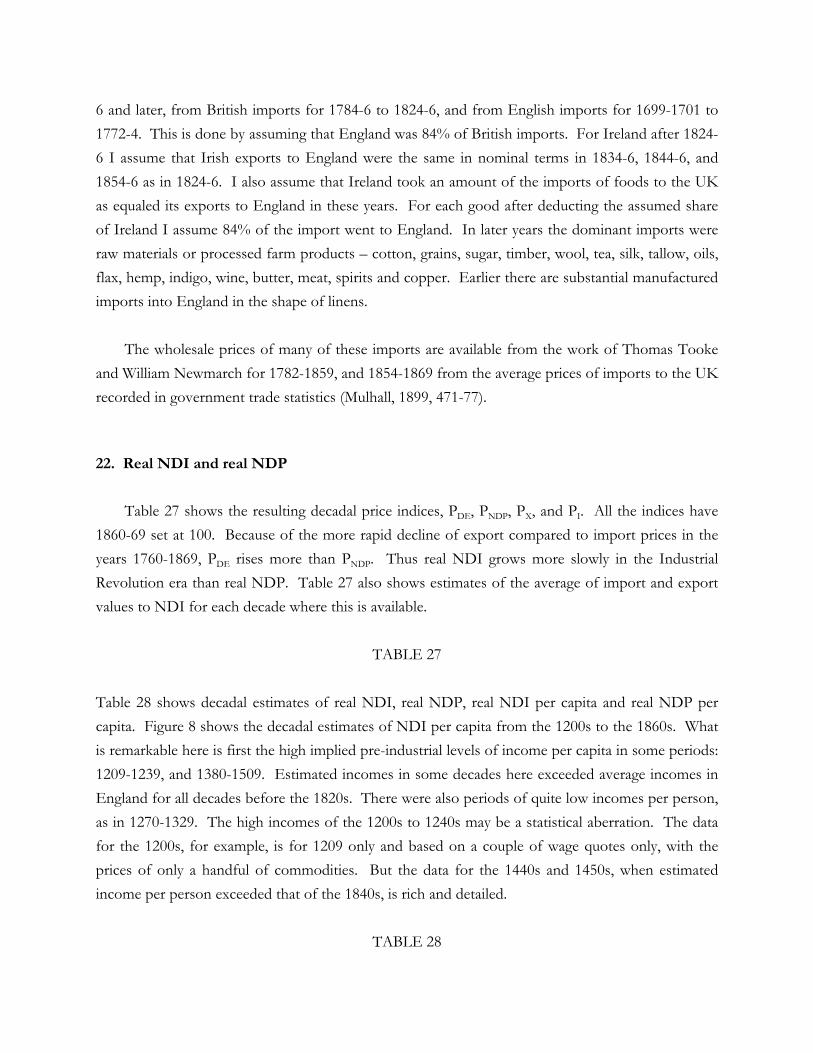
Table 28 shows decadal estimates of real NDI, real NDP, real NDI per capita and real NDP per
capita. Figure 8 shows the decadal estimates of NDI per capita from the 1200s to the 1860s. What
is remarkable here is first the high implied pre-industrial levels of income per capita in some periods:
1209-1239, and 1380-1509. Estimated incomes in some decades here exceeded average incomes in
England for all decades before the 1820s. There were also periods of quite low incomes per person,
as in 1270-1329. The high incomes of the 1200s to 1240s may be a statistical aberration. The data
for the 1200s, for example, is for 1209 only and based on a couple of wage quotes only, with the
prices of only a handful of commodities. But the data for the 1440s and 1450s, when estimated
income per person exceeded that of the 1840s, is rich and detailed.
TABLE 28
The implied estimated growth rates of NDP per capita in the Industrial Revolution era are low
relative even to the relatively pessimistic estimates of Knick Harley and Nick Crafts from primal
sources. Thus over the hundred years from the 1760s to the 1860s real NDP per capita increased by
60%, at an average annual rate of 0.47%. Crafts and Harley estimate an annual growth rate of GDP
per person in this interval of 0.55% (Crafts and Harley, 1992). This in turn would imply an overall
increase of GDP per person of 73% in these years.
Growth measured in terms of national income was even slower because of the decline in the
terms of trade. Thus income per person (NNI) increased by only 48% over the hundred years
between the 1760s and the 1860s, implying an annual growth rate of only 0.39%. Figure 8, showing
income per person in England from 1200s to 1860s, implies that this makes the discontinuity of the
Industrial Revolution less clear. Was the Industrial Revolution just the acceleration of a period of
slow growth beginning around 1600? Figure 8: NDI/N, 1200s-1860s
0
20
40
60
80
100
120
1200 1300 1400 1500 1600 1700 1800
Rea
l NN
I/N
(186
0s =
100)
23. Cost of Living Index and Real Wages
One big issue in the Industrial Revolution era is the standard of living of workers. That
requires a cost of living index which has different weights from the national price index. The cost of
living index aimed for here is one that applies to the average wage earner, not the poorest such as
agricultural workers (such an index is reported for agricultural workers in Clark, 2001, and Clark,
2007b).
Table 29 shows the weights in the principal components of the workers cost of living index for
various periods. The principal difference here is the larger weight given to food, and the much
smaller weight given to services. These weights are derived from Clark (2001, 2005), which reports
contemporary surveys of worker consumption patterns in England, mainly for the years 1789-1869.
Within the sub-indices the weights also differ. Within the food category, starches are given greater
weight and meat and dairy products less (table 30). In drink, beer is much more important than
wine in the cost of living index (table 31). In clothing, silk is excluded from the cost of living index.
TABLES 29, 30, 31
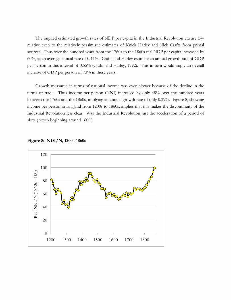
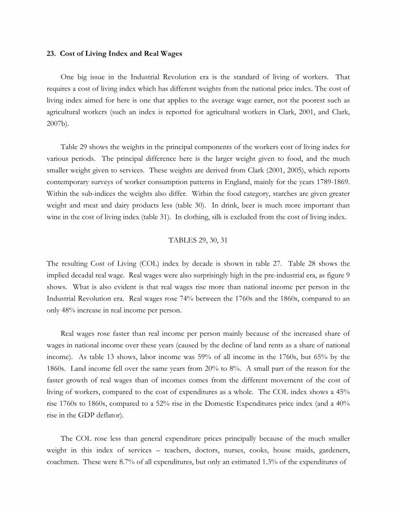
The resulting Cost of Living (COL) index by decade is shown in table 27. Table 28 shows the
implied decadal real wage. Real wages were also surprisingly high in the pre-industrial era, as figure 9
shows. What is also evident is that real wages rise more than national income per person in the
Industrial Revolution era. Real wages rose 74% between the 1760s and the 1860s, compared to an
only 48% increase in real income per person.
Real wages rose faster than real income per person mainly because of the increased share of
wages in national income over these years (caused by the decline of land rents as a share of national
income). As table 13 shows, labor income was 59% of all income in the 1760s, but 65% by the
1860s. Land income fell over the same years from 20% to 8%. A small part of the reason for the
faster growth of real wages than of incomes comes from the different movement of the cost of
living of workers, compared to the cost of expenditures as a whole. The COL index shows a 45%
rise 1760s to 1860s, compared to a 52% rise in the Domestic Expenditures price index (and a 40%
rise in the GDP deflator).
The COL rose less than general expenditure prices principally because of the much smaller
weight in this index of services – teachers, doctors, nurses, cooks, house maids, gardeners,
coachmen. These were 8.7% of all expenditures, but only an estimated 1.3% of the expenditures of
Figure 9: Real Wages by Decade, 1200s-1860s
Figure 10: Real wages and Real Income per Capita by Decade, 1760-1869
0
20
40
60
80
100
120
1200 1300 1400 1500 1600 1700 1800
Rea
l Wag
e (1
860s
=10
0)
0
20
40
60
80
100
120
1760 1780 1800 1820 1840 1860
Rea
l GN
I/N
, Wag
e (1
860s
=10
0)
Real Wage
Real Income per Capita
workers. Because urban wages rose by 148% in these years, which was more any other expenditure
price, the expenditure deflator rose by more than the cost of living of workers. Indeed the higher
weight given to services explains most of the difference in aggregate between these two indices over
these years. The weights for other items did differ substantially, as table 32 shows. The poor ate
much more grain and potato products. But here the rate of price increase did not differ much from
the average good. The workers drank more beer, whose price increase was more than the average,
but in compensation richer consumers were assumed to drink more wine. But since there were so
many changes in weights and relative price movements, as table 32 shows, mostly these effects
cancelled out in terms of the rise of the COL versus PDE.
TABLE 32
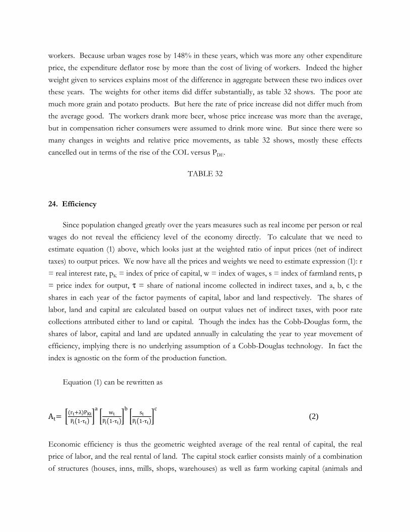
24. Efficiency
Since population changed greatly over the years measures such as real income per person or real
wages do not reveal the efficiency level of the economy directly. To calculate that we need to
estimate equation (1) above, which looks just at the weighted ratio of input prices (net of indirect
taxes) to output prices. We now have all the prices and weights we need to estimate expression (1): r
= real interest rate, pK = index of price of capital, w = index of wages, s = index of farmland rents, p
= price index for output, τ = share of national income collected in indirect taxes, and a, b, c the
shares in each year of the factor payments of capital, labor and land respectively. The shares of
labor, land and capital are calculated based on output values net of indirect taxes, with poor rate
collections attributed either to land or capital. Though the index has the Cobb-Douglas form, the
shares of labor, capital and land are updated annually in calculating the year to year movement of
efficiency, implying there is no underlying assumption of a Cobb-Douglas technology. In fact the
index is agnostic on the form of the production function.
Equation (1) can be rewritten as At rt λ PKtPt 1-τt
a wtPt 1-τtb stPt 1-τt
c (2)
Economic efficiency is thus the geometric weighted average of the real rental of capital, the real
price of labor, and the real rental of land. The capital stock earlier consists mainly of a combination
of structures (houses, inns, mills, shops, warehouses) as well as farm working capital (animals and

grains) and non-farm working capital. It thus seems reasonable to assume that the price of this
capital moves in line with general prices in the economy, so that PKt = Pt . This assumption implies
that the capital goods sector experienced as much efficiency growth as the rest of the economy. In
implementing this index of productivity the question arises about what value to give to λ, the risk
premium on capital. Since early interest rates are high, the greater is λ, the smaller will be the capital
cost contribution to productivity levels in earlier years. But the capital stock was a combination of
houses, with little risk premium on their return, farm capital with an intermediate risk premium, and
commercial capital with a significant risk premium. As a compromise I take λ=3%.
Figure 11 shows productivity from 1209 to the 1860s calculated with the expenditure prices
from England. It shows the overall efficiency of the economy in translating inputs into real income,
whether the purchases were produced domestically or abroad. The decades 1200-9 to 1280-9 are
shown as a dotted line to emphasize how much more tentative the estimates are for these decades
Figure 12 shows productivity over the same period calculated based on the prices of English
output only. The effect of using the NDP price index in the years before 1870 is shows mainly in
the greater rise of efficiency in the Industrial Revolution period, the 1780s to 1860s. Measured using
expenditure prices the productivity growth rate is 0.37 percent per year from the 1760s to 1860s.
Measured using expenditure prices the productivity growth rate for the 1760s to 1860s is 0.37
percent per year. This 0.45 for productivity growth measured on the basis of output prices is
similar, but again below, what has been regarded as the pessimistic rate of 0.55 percent per year
calculated by Crafts and Harley (1992), which is done on a GDP basis. But I will discuss further
below why the expenditure based index seems more appropriate. Table 32 shows both these sets of
productivity measures by decade.
TABLE 33
Figure 13 shows why the measured efficiency of the economy moves as it does from the 1200s
to 1860s, by looking at the components of equation (2) for efficiency. The reason that measured
efficiency is so unexpectedly high in the years before 1350, despite the relatively low levels of output
per person, is the high calculated underlying real interest rate in this epoch. Real interest rates in the
thirteenth century were 2.5 times as great as in the eighteenth and nineteenth centuries. Since I have
assumed that in both farming and non-farm activities there was a fixed ration for working capital to
output, this raises the weight of capital, a, in the productivity equation (1) in these years, since the
share of capital in all payments is assumed to rise. Had I assumed that capital entered the
production function in a Cobb-Douglas fashion, with a fixed share of payments to factors going to
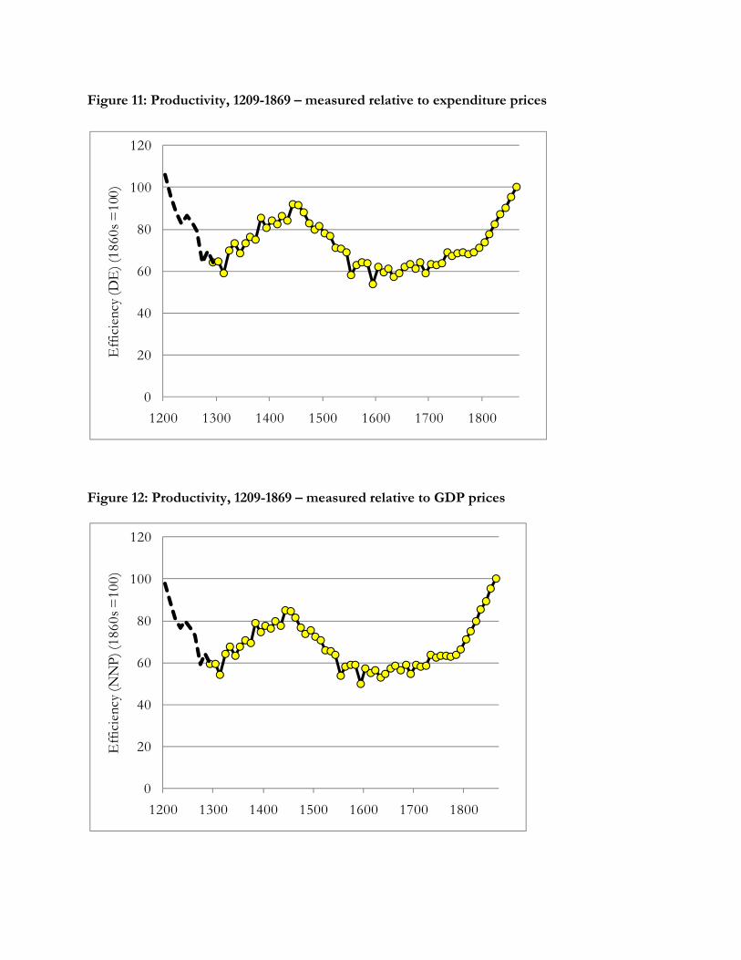
Figure 11: Productivity, 1209-1869 – measured relative to expenditure prices
Figure 12: Productivity, 1209-1869 – measured relative to GDP prices
0
20
40
60
80
100
120
1200 1300 1400 1500 1600 1700 1800
Eff
icie
ncy
(DE
) (18
60s =
100)
0
20
40
60
80
100
120
1200 1300 1400 1500 1600 1700 1800
Eff
icie
ncy
(NN
P) (
1860
s =
100)
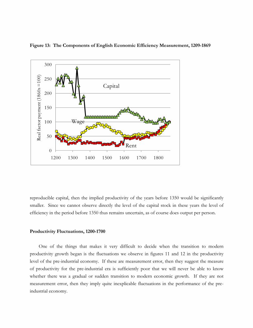
Figure 13: The Components of English Economic Efficiency Measurement, 1209-1869
reproducible capital, then the implied productivity of the years before 1350 would be significantly
smaller. Since we cannot observe directly the level of the capital stock in these years the level of
efficiency in the period before 1350 thus remains uncertain, as of course does output per person.
Productivity Fluctuations, 1200-1700
One of the things that makes it very difficult to decide when the transition to modern
productivity growth began is the fluctuations we observe in figures 11 and 12 in the productivity
level of the pre-industrial economy. If these are measurement error, then they suggest the measure
of productivity for the pre-industrial era is sufficiently poor that we will never be able to know
whether there was a gradual or sudden transition to modern economic growth. If they are not
measurement error, then they imply quite inexplicable fluctuations in the performance of the pre-
industrial economy.
0
50
100
150
200
250
300
1200 1300 1400 1500 1600 1700 1800
Rea
l fac
tor p
aym
ent (
1860
s =10
0)
Capital
Wage
Rent
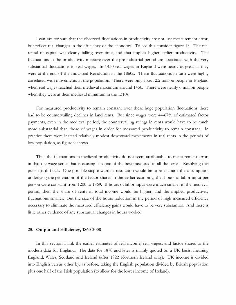
I can say for sure that the observed fluctuations in productivity are not just measurement error,
but reflect real changes in the efficiency of the economy. To see this consider figure 13. The real
rental of capital was clearly falling over time, and that implies higher earlier productivity. The
fluctuations in the productivity measure over the pre-industrial period are associated with the very
substantial fluctuations in real wages. In 1450 real wages in England were nearly as great as they
were at the end of the Industrial Revolution in the 1860s. These fluctuations in turn were highly
correlated with movements in the population. There were only about 2.2 million people in England
when real wages reached their medieval maximum around 1450. There were nearly 6 million people
when they were at their medieval minimum in the 1310s.
For measured productivity to remain constant over these huge population fluctuations there
had to be countervailing declines in land rents. But since wages were 44-67% of estimated factor
payments, even in the medieval period, the countervailing swings in rents would have to be much
more substantial than those of wages in order for measured productivity to remain constant. In
practice there were instead relatively modest downward movements in real rents in the periods of
low population, as figure 9 shows.
Thus the fluctuations in medieval productivity do not seem attributable to measurement error,
in that the wage series that is causing it is one of the best measured of all the series. Resolving this
puzzle is difficult. One possible step towards a resolution would be to re-examine the assumption,
underlying the generation of the factor shares in the earlier economy, that hours of labor input per
person were constant from 1200 to 1869. If hours of labor input were much smaller in the medieval
period, then the share of rents in total income would be higher, and the implied productivity
fluctuations smaller. But the size of the hours reduction in the period of high measured efficiency
necessary to eliminate the measured efficiency gains would have to be very substantial. And there is
little other evidence of any substantial changes in hours worked.
25. Output and Efficiency, 1860-2008
In this section I link the earlier estimates of real income, real wages, and factor shares to the
modern data for England. The data for 1870 and later is mainly quoted on a UK basis, meaning
England, Wales, Scotland and Ireland (after 1922 Northern Ireland only). UK income is divided
into English versus other by, as before, taking the English population divided by British population
plus one half of the Irish population (to allow for the lower income of Ireland).
Real GDP per person: Feinstein gives for 1860-1920 real GDP per capita for Great Britain
(Feinstein, 1972, T118-9). This series is continued for England 1920-1948 by deflating nominal
GDP per person for the UK by Feinstein’s GDP deflator (Feinstein, 1972, T5-9, T132-3). For
1948-2008 the Office of National Statistics reports real GDP per capita (UK, Office of National
Statistics). The decadal averages for this series are reported in the second column of table 34. This
is thus a continuation of the columns in table 28 giving measures of real NNI per capita and real
GDP per capita for the 1860s and earlier.
TABLE 34
Farmland rent share: Net domestic income for England 1860-2007 is calculated by reducing UK
net domestic income to an English basis. Total farmland rents for England 1860-1914 are from
Stamp, 1922, 49, Engand and Wales, adjusted to an English basis. This Stamp series is projected on
to 1944 using the movement of UK farmland rents reported in Feinstein, 1972, T60. For 1944-2004
the Department of Environment, Food, and Rural Affairs (DEFRA), reports a series “Agricultural
Land Sales and Prices in England” which gives prices per acre/hectare. This are converted into
rents per acre in 1945-1967 using a return rate of 3%, and multiplied by an assumed 28 m. acres of
farmland in England to give total rents. For 1968-2007 DEFRA reports a series on land tenancy
rentals per hectare (normed to the average of Full Annual Tenancy and Farm Business Tenancy
leases). Again these are multiplied by an assumed 28 m. acres farm area to give total farm rents.
The implied share of rents in national income in England are shown in table 34.
Share of Wages: Feinstein reports both wages and salaries and income from self employment for
the UK 1860-1947 (Feinstein, 1972, p. T4-9). Income from self-employment is assumed throughout
to be half labor income. This is divided by UK net domestic income minus expenditure taxes (less
subsidies). For 1948-2008 the share of wages is calculated in the same way from the series reported
by the Office of National Statistics.
Urban Site Rents: The Blue Books (Office of National Statistics) give from 1987-2007 the value
for the UK of dwellings and other buildings (including and excluding the land value). From this can
be inferred the capital value of urban site rents. Since site rents exhibit no depreciation these are
converted into site rents by multiplying them by an assumed rate of return (excluding capital gains)
of 3% 1987-1996 (the rental return on farmland averaged only 2.8% between 1968 and 2007). From
1996-2005 house prices in England rose by 170%, while house rents rose by 34%. If the rental
return on housing was 3% in 1996, then by 2005 it was 1.5%. So for these years the capitalized site
values are converted into implicit rentals by the current implied rental on housing. This data
suggests that urban site rentals represented then about 4% of total incomes (and about 45% of the
value of dwellings and other buildings).
Singer (1941) estimates urban site values in England and Wales, 1845-1910 from the movement
of construction costs versus tax assessments. The weakness in this estimate, however is that he has
to make an assumption about the share of site rents in property rentals in 1845, which he assumes
then is only 8.2% of building rents. This gives site rents 1860-1910.
Site rents 1947-1986 are estimated from the relative movement of the total average house values
(constructed as number of households×average house price) compared to the average value of the
reproducible housing capital stock reported by the Office of National Statistics. The house price
series continues back to 1930. It is used to project site values back to then by assuming the same
proportion of house values were site rents throughout the 1930-1947 period.
Share of Capital: This was constructed as a residual so that the shares of land, labor, urban site
rents and capital summed to 1.
Real Wage and Skill Premium: The real wage series here is that of Clark (2005), and covers an
average of building workers and craftsmen. Real wages are calculated as the average of nominal
wages per 10 hours for building trademen and for building laborers, deflated by Feinstein’s cost of
living index (until 1993) (Feinstein, 1995), and thereafter by the retail price index from the Office of
National Statistics. The skill premium is the differential of the wage of craftsmen to workers.
Economic Efficiency: The decline of land rents to a tiny share of national income since 1860, and
the relative constancy of the rate of return on capital, mean that the equation (1) for calculating
economic efficiency since 1860 reduces to the simple expression,
(3)
The last column of table 34 gives this simple measure of economic efficiency by decade from the
1860s to the 2000s, with the 1860s set at 100. Because the magnitude of b varies over time between
0.65 and 0.80 the index is constructed by periodically changing the weights periodically and chaining
the resulting indices. This is a continuation of the efficiency indices constructed in table 33. Figure
14 shows the picture of the efficiency of the English economy from the 1200s to the 2000s.
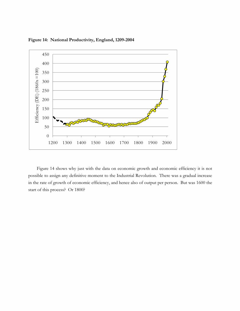
Figure 14: National Productivity, England, 1209-2004
Figure 14 shows why just with the data on economic growth and economic efficiency it is not
possible to assign any definitive moment to the Industrial Revolution. There was a gradual increase
in the rate of growth of economic efficiency, and hence also of output per person. But was 1600 the
start of this process? Or 1800?
0
50
100
150
200
250
300
350
400
450
1200 1300 1400 1500 1600 1700 1800 1900 2000
Eff
icie
ncy
(DE
) (18
60s =
100)
Bibliography Albert, W. 1972. The Turnpike Road System in England 1663-1840. Cambridge: Cambridge University
Press. Allen, Robert C. 2008. “Review of A Farewell to Alms.” Journal of Economic Literature. Barney, John M. 1999. “Shipping in the Port of King’s Lynn, 1702-1800” Journal of Transport History,
20(2): 126-140. Bogart, Dan. 2005. “Did Turnpike Trusts Increase Transportation Investment in Eighteenth-
Century England.” Journal of Economic History, 65(June): 439-468. Bowley, A. L. 1898. “The Statistics of Wages in the United Kingdom during the last Hundred
Years. Part I. Agricultural Wages,” Journal of the Royal Statistical Society, 61: 702-722. Broadberry, Stephen, Bruce Campbell, et al. 2009. “British Economic Growth, 1300-1850: Some
Preliminary Estimates.” University of Warwick. Clark, Gregory. 2007a. “The Long March of History: Farm Wages, Population and Economic
Growth, England 1209-1869” Economic History Review.
Clark, Gregory. 2007b. A Farewell to Alms: A Brief Economic History of the World. Princeton: Princeton
University Press.
Clark, Gregory. 2005. “The Condition of the Working-Class in England, 1209-2004” Journal of
Political Economy, 113(6) (December, 2005): 1307-1340.
Clark, Gregory. 2002a. "Farmland Rental Values and Agrarian History: England and Wales, 1500-
1912" European Review of Economic History, 6(3) (December 2002): 281-309. Clark, Gregory. 2002b. "Shelter from the Storm: Housing and the Industrial Revolution, 1550-
1912" Journal of Economic History, 62(2) (June 2002).
Clark, Gregory. 2001a. “Farm wages and living standards in the Industrial Revolution: England,
1670-1869.” Economic History Review.
Clark, Gregory. 2001b. “Markets and Economic Growth: The Grain Market of Medieval
England.” Working Paper, UC-Davis.
Clark, Gregory. 1998a. “Land Hunger: Land as a Commodity and as a Status Good in England,
1500-1910,” Explorations in Economic History, 35(1) (January): 59-82.
Clark, Gregory. 1998b. “The Reports of the Charity Commission as a Source in Economic
History.” Research in Economic History 18.
Clark, Gregory. 1996. “The Political Foundations of Modern Economic Growth: England, 1540-
1800,” Journal of Interdisciplinary History, 26 (Spring): 563-588.
Clark, Gregory. 1988. "The Cost of Capital and Medieval Agricultural Technique," Explorations in
Economic History, 25 (July): 265-294.
Clark, Gregory, Michael Huberman and Peter Lindert. 1995. “A British Food Puzzle, 1770-1850,”
Economic History Review, 48(2): 215-237.
Clark, Gregory and Patricia Levin. 2001. “How different was the Industrial Revolution? The
Revolution in Printing, 1350-1869.” Working Paper, University of California, Davis.
Clark, Gregory and Van Der Werf, Ysbrand. 1998. "Work in Progress? The Industrious
Revolution". Journal of Economic History 58 (3): 830–843.
Chubb, Harry. 1876. “The Supply of Gas to the Metropolis.” Journal of the Statistical Society of
London, Vol. 39, No. 2 (Jun): 350-380
Crafts, N. F. R. 1985. British Economic Growth During the Industrial Revolution. New York: Oxford
University Press.
Crafts, N.F.R., and C. K. Harley. 1992. "Output Growth and the Industrial Revolution: A
Restatement of the Crafts-Harley View." Economic History Review 45:703-730.
Deane, Phyllis, and W. A. Cole. 1967. British Economic Growth, 1688-1959. 2d ed. Cambridge:
Cambridge University Press.
Davis, Ralph. 1956. “Seamen's Sixpences: An Index of Commercial Activity, 1697-1828” Economica,
23(92): 328-43.
Davis, Ralph. 1957. “Earnings of Capital in the English Shipping Industry, 1670-1730” Journal of
Economic History, 17(3): 409-25.
Davis, Ralph. 1962. “English Foreign Trade, 1700-1774” Economic History Review, 15(2): 285-303.
Davis, Ralph. 1979. The Industrial Revolution and British Overseas Trade. Leicester: Leicester University
Press.
De Vries, Jan. 1994. “The Industrial Revolution and the Industrious Revolution.” Journal of
Economic History, 54: 249-270.
De Vries, Jan and Ad van der Woude. 1997. The first modern economy : success, failure, and perseverance of
the Dutch economy, 1500-1815. Cambridge: Cambridge University Press.
De Vries, Jan. 2000. “Dutch Economic Growth in Comparative Historical Perspective, 1500-2000.
De Economist, 148 (4): 443-467.
De Vries, Jan. 2008. The Industrious Revolution: Consumer Behavior and the Household Economy, 1650 to the
Present. Cambridge: Cambridge University Press.
Dietz, Frederick C. 1921. English Government Finance, 1485-1558. New York: Barnes and Noble.
Dietz, Frederick C. 1932. English Government Finance, 1558-1641. New York: Barnes and Noble.
Dyer, Christopher. 1988. “Changes in Diet in the Late Middle Ages: the Case of Harvest Workers.”
Agricultural History Review, 36(1): 21-37.
Falkus, M. E. 1982. “The Early Development of the British Gas Industry, 1790-1815.” Economic
History Review, New Series, Vol. 35, No. 2 (May): 217-234.
Feinstein, Charles H. 1972. National Income, Expenditure and Output of the United Kingdom, 1855-1965.
Cambridge: Cambridge University Press.
Feinstein, Charles H. 1988. “National Statistics, 1760-1920” in Charles H. Feinstein and Sidney
Pollard, Studies in Capital Formation in the United Kingdom, 1750-1920. Oxford: Clarendon
Press, 258-404.
Feinstein, Charles H. 1995. “Changes in Nominal Wages, the Cost of Living and Real Wages in the
United Kingdom over Two Centuries.” in P Scholliers and V. Zamagni (eds.), Labour’s
Reward: Real Wages and Economic Change in 19th- and 20th-Century Europe. Aldershot, Hants:
Edward Elgar.
Feinstein, Charles H. 1998a. “Pessimism Perpetuated: Real Wages and the Standard of Living in
Britain During and After the Industrial Revolution.” Journal of Economic History, 58 (3) (Sept.),
625-658.
Feinstein, Charles H. 1998b. “Wage-Earnings in Great Britain during the Industrial Revolution.” In
Iain Begg and S. G. B. Henry, Applied Economics and Public Policy. Cambridge: Cambridge
University Press.
Flinn, Michael W. 1984. The History of the British Coal Industry. Vol. 2,1700-1830. Oxford. Clarendon
Press.
Ginarlis, John and Sidney Pollard. 1988. “Roads and Waterways, 1750-1850.” In Charles H.
Feinstein and Sidney Pollard, Studies in Capital Formation in the United Kingdom, 1750-1920.
Oxford: Clarendon Press, 182-224.
Grimwade, M. E. 1979. Index of the Probate Records of the Court of the Archdeacon of Suffolk, 1444-1700.
London: The British Record Society.
Graham, Gerald S. 1956. “The Ascendancy of the Sailing Ship 1850-85” Economic History Review,
New Series, 9(1): 74-88.
Harley, Knick. 1988. “Ocean Freight Rates and Productivity, 1740-1913: The Primacy of
Mechanical Invention Reaffirmed” Journal of Economic History, 48(4) (Dec.):851-76.
Harley, Knick. 1993. “Reassessing the Industrial Revolution: A Macro View,” in Joel Mokyr (ed.),
The British Industrial Revolution: An Economic Assessment (Boulder, Colorado: Westview Press,
1993), 227-266.
Harley, Knick. 1997. “Cotton Textile Prices and the Industrial Revolution,” Working Paper,
University of Western Ontario, February 1997.
Harris, G. L. 1975. King, Parliament, and Public Finance in Medieval England to 1369. Oxford:
Clarendon Press.
Hatcher, John. 1993. The History of the British Coal Industry, Vol. 1, Before 1700: Towards the Age of Coal.
Oxford: Clarendon Press.
Jastram, Roy W. 1981. Silver: The Restless Metal. New York: John Wiley and Sons.
Levi, Leone. 1867. Wages and Earnings of the Working Classes. London: John Murray.
Lindert, Peter H. 1980. "English Occupations, 1670-1811." Journal of Economic History 40:685-712.
Matthews, Derek. 1986. “Laissez-faire and the London Gas Industry in the Nineteenth Century:
Another Look.” The Economic History Review, New Series, 39(2) (May): 244-263
Matthews, William. 1832. An historical sketch of the origin and progress of gas-lighting . London: Simpkin
and Marshall.
Mitchell, B. R. and Phyllis Deane. 1971. Abstract of British Historical Statistics. Cambridge: Cambridge
University Press.
Mitchell, B. R. 1988. British Historical Statistics. Cambridge: Cambridge University Press.
Mulhall, Michael G. 1899. The Dictionary of Statistics. London: Routledge.
Parliamentary Papers. 1803-4. Report from the Committee on the London Bakers Petition.
Parliamentary Papers. 1812-13. Report from the Committee on the Petition of Certain County Bakers.
Parliamentary Papers. 1852-3. 1851 Census. Ages, Civil Conditions Occupations and Birthplaces. Part I.
Vol. lxxxviii Part I, 1.
Pawson, Eric. 1977. Transport and Economy: The Turnpike Roads of Eighteenth Century Britain. London:
Academic Press.
Pollard, Sydney. 1988. “The Insurance Policies” in in Charles H. Feinstein and Sidney Pollard,
Studies in Capital Formation in the United Kingdom, 1750-1920. Oxford: Clarendon Press, 225-
257.
Prados de la Escosura , Leandro. 2000. “International Comparisons of Real Product, 1820-1990:
An Alternative Data Set” Explorations in Economic History, 37(1): 1-41.
Shaw-Taylor, Leigh and E.A. Wrigley. 2008. “The Occupational Structure of England c. 1750-1871:
A Preliminary Report.” Cambridge, England: Cambridge Group for the History of
Population and Social Structure.
Singer, H. W. 1941. “An Index of Urban Land Rents and House Rents in England and Wales,
1845-1913” Econometrica, 9(3/4): 221-230
Smits, Jan-Pieter, Edwin Horlings, and Jan Luiten van Zanden. 1999. Dutch GNP and Its Components,
1800-1913. Groningen Growth and Development Center, Monograph Series, #5.
Stamp, Josiah. 1922. British Incomes and Property. London: King and Son.
Squarey, Elias P. 1878. “Farm Capital” Journal of the Royal Agricultural Society of England, Second
Series, 14, 425-444.
Terry, Schuyler B. 1914. The Financing of the Hundred Years’ War, 1337-1360. London: Constable and
Co.
Tomson, James. 1847. “Acount of Hall Farm, near Sevenoaks, Kent.” Journal of the Royal
Agricultural Society of England, 8, 33-46.
Ville, Simon P. 1990. English shipowning during the industrial revolution: Michael Henley and Son, London
Shipowners, 1770-1830. Manchester: Manchester University Press.
Voth, Hans-Joachim. 2001a. Time and Work in England, 1750-1830. Oxford: Oxford University Press.
Voth, Hans-Joachim. 2001b. “The Longest Years: New Estimates of Labor Input in England,
1760-1830.” Journal of Economic History, 61(4): 1065-82.
Wratislaw, Charles. 1861. “The Amount of Capital Required for the Profitable Operation of a
Mixed Arable and Pasture Farm in a Midland County.” Journal of the Royal Agricultural
Society of England, Second Series, 14, 425-444.
Wrigley, E. A. 1985. "Urban Growth and Agricultural Change: England and the Continent in the
Early Modern Period." Journal of Interdisciplinary History 15:683-728.
Wrigley, E. A., R. S. Davies, J. E. Oeppen, and R. S. Schofield. 1997. English Population History from
Family Reconstruction: 1580-1837. Cambridge; New York: Cambridge University Press.
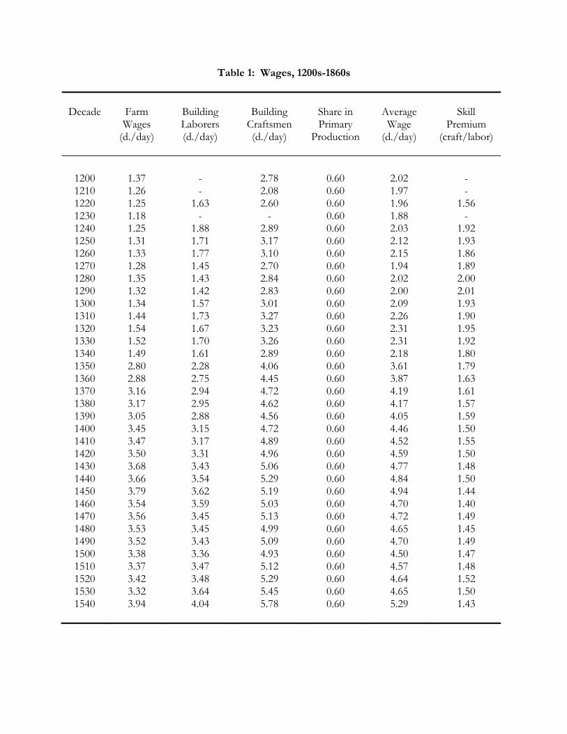
Table 1: Wages, 1200s-1860s
Decade
Farm Wages
(d./day)
Building Laborers (d./day)
Building
Craftsmen (d./day)
Share in Primary
Production
Average
Wage (d./day)
Skill
Premium (craft/labor)
1200 1.37 - 2.78 0.60 2.02 - 1210 1.26 - 2.08 0.60 1.97 - 1220 1.25 1.63 2.60 0.60 1.96 1.56 1230 1.18 - - 0.60 1.88 - 1240 1.25 1.88 2.89 0.60 2.03 1.92 1250 1.31 1.71 3.17 0.60 2.12 1.93 1260 1.33 1.77 3.10 0.60 2.15 1.86 1270 1.28 1.45 2.70 0.60 1.94 1.89 1280 1.35 1.43 2.84 0.60 2.02 2.00 1290 1.32 1.42 2.83 0.60 2.00 2.01 1300 1.34 1.57 3.01 0.60 2.09 1.93 1310 1.44 1.73 3.27 0.60 2.26 1.90 1320 1.54 1.67 3.23 0.60 2.31 1.95 1330 1.52 1.70 3.26 0.60 2.31 1.92 1340 1.49 1.61 2.89 0.60 2.18 1.80 1350 2.80 2.28 4.06 0.60 3.61 1.79 1360 2.88 2.75 4.45 0.60 3.87 1.63 1370 3.16 2.94 4.72 0.60 4.19 1.61 1380 3.17 2.95 4.62 0.60 4.17 1.57 1390 3.05 2.88 4.56 0.60 4.05 1.59 1400 3.45 3.15 4.72 0.60 4.46 1.50 1410 3.47 3.17 4.89 0.60 4.52 1.55 1420 3.50 3.31 4.96 0.60 4.59 1.50 1430 3.68 3.43 5.06 0.60 4.77 1.48 1440 3.66 3.54 5.29 0.60 4.84 1.50 1450 3.79 3.62 5.19 0.60 4.94 1.44 1460 3.54 3.59 5.03 0.60 4.70 1.40 1470 3.56 3.45 5.13 0.60 4.72 1.49 1480 3.53 3.45 4.99 0.60 4.65 1.45 1490 3.52 3.43 5.09 0.60 4.70 1.49 1500 3.38 3.36 4.93 0.60 4.50 1.47 1510 3.37 3.47 5.12 0.60 4.57 1.48 1520 3.42 3.48 5.29 0.60 4.64 1.52 1530 3.32 3.64 5.45 0.60 4.65 1.50 1540 3.94 4.04 5.78 0.60 5.29 1.43
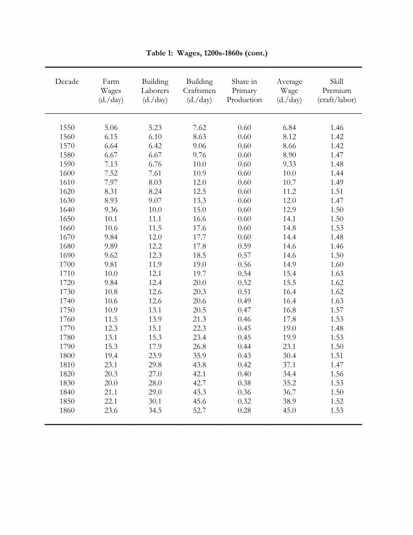
Table 1: Wages, 1200s-1860s (cont.)
Decade
Farm Wages
(d./day)
Building Laborers (d./day)
Building
Craftsmen (d./day)
Share in Primary
Production
Average
Wage (d./day)
Skill
Premium (craft/labor)
1550 5.06 5.23 7.62 0.60 6.84 1.46 1560 6.15 6.10 8.63 0.60 8.12 1.42 1570 6.64 6.42 9.06 0.60 8.66 1.42 1580 6.67 6.67 9.76 0.60 8.90 1.47 1590 7.13 6.76 10.0 0.60 9.33 1.48 1600 7.52 7.61 10.9 0.60 10.0 1.44 1610 7.97 8.03 12.0 0.60 10.7 1.49 1620 8.31 8.24 12.5 0.60 11.2 1.51 1630 8.93 9.07 13.3 0.60 12.0 1.47 1640 9.36 10.0 15.0 0.60 12.9 1.50 1650 10.1 11.1 16.6 0.60 14.1 1.50 1660 10.6 11.5 17.6 0.60 14.8 1.53 1670 9.84 12.0 17.7 0.60 14.4 1.48 1680 9.89 12.2 17.8 0.59 14.6 1.46 1690 9.62 12.3 18.5 0.57 14.6 1.50 1700 9.81 11.9 19.0 0.56 14.9 1.60 1710 10.0 12.1 19.7 0.54 15.4 1.63 1720 9.84 12.4 20.0 0.52 15.5 1.62 1730 10.8 12.6 20.3 0.51 16.4 1.62 1740 10.6 12.6 20.6 0.49 16.4 1.63 1750 10.9 13.1 20.5 0.47 16.8 1.57 1760 11.5 13.9 21.3 0.46 17.8 1.53 1770 12.3 15.1 22.3 0.45 19.0 1.48 1780 13.1 15.3 23.4 0.45 19.9 1.53 1790 15.3 17.9 26.8 0.44 23.1 1.50 1800 19.4 23.9 35.9 0.43 30.4 1.51 1810 23.1 29.8 43.8 0.42 37.1 1.47 1820 20.3 27.0 42.1 0.40 34.4 1.56 1830 20.0 28.0 42.7 0.38 35.2 1.53 1840 21.1 29.0 43.3 0.36 36.7 1.50 1850 22.1 30.1 45.6 0.32 38.9 1.52 1860 23.6 34.5 52.7 0.28 45.0 1.53

Table 2: Assumed sectoral employment distribution
Year
Share primary sector assumed
here
Broadberry et al.
(Agricultural Population)
Share in Wills
(primary sector)
1851 .34 - 0.36 1817 .42 - 0.44 1755 .47 - 0.45 1700 .48 .54 0.48 1680 .50 - 0.50 1600 .60 .70 0.60
1560/70 .60 - 0.60 1520/30 .60 .75 -
1380 .60 .76 - 1300 .60 .79 -
Notes: Broadberry et al. (2009), table 18, Shaw-Taylor, Leigh and E.A. Wrigley (2008).
Table 3: Labor Income 1866 from Levi
Category
Number
1860-9 (m)
Wage per day,
1866 (d.)
Male-
Equivalents
Total
Earnings, 1866 (£ m.)
Men 20-64
5.37
45
1.00
302
Men, < 20 1.36 13 0.29 22 Women 20-64 2.45 25 0.56 77 Women <20 0.90 17 0.38 19 All
10.08
32.1
0.71
420

Table 4: Alternative population estimates, England, 1300-1600
Year
Broadberry et al. population (m.)
Clark (2007a)
population (m.)
Ratio
1300 4.25 5.32 1.25 1348 3.83 4.48 1.17 1351 2.56 3.54 1.38 1380 2.37 2.98 1.26 1520 2.20 2.87 1.30 1600 4.12 4.28 1.04
Sources: Broadberry, Campbell et al. (2009), table 18.
Table 5: Broadberry et al.’s assumptions about farm labor inputs
Date
Assumed work days per farm
family
Farm families
(m.)
Farm output
(index)
Output per work day (index)
1250 315 0.68 1.00 1.00 1300 381 0.74 1.17 0.89 1380 331 0.40 1.07 1.72 1450 266 0.38 0.94 1.97 1600 404 0.64 1.51 1.25 1700 405 0.62 2.18 1.86 1800 473 0.69 2.52 1.64 1850 539 0.73 4.66 2.51 Sources: Broadberry, Campbell et al. (2009), table 24.
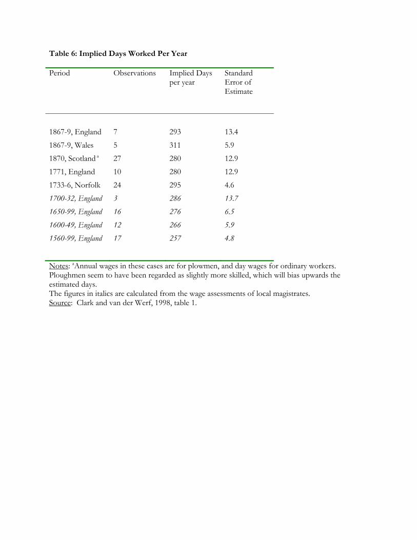
Table 6: Implied Days Worked Per Year Period Observations Implied Days
per year
Standard Error of Estimate
1867-9, England 7 293 13.4
1867-9, Wales 5 311 5.9
1870, Scotland a 27 280 12.9
1771, England 10 280 12.9
1733-6, Norfolk 24 295 4.6
1700-32, England 3 286 13.7
1650-99, England 16 276 6.5
1600-49, England 12 266 5.9
1560-99, England 17 257 4.8
Notes: aAnnual wages in these cases are for plowmen, and day wages for ordinary workers. Ploughmen seem to have been regarded as slightly more skilled, which will bias upwards the estimated days. The figures in italics are calculated from the wage assessments of local magistrates. Source: Clark and van der Werf, 1998, table 1.
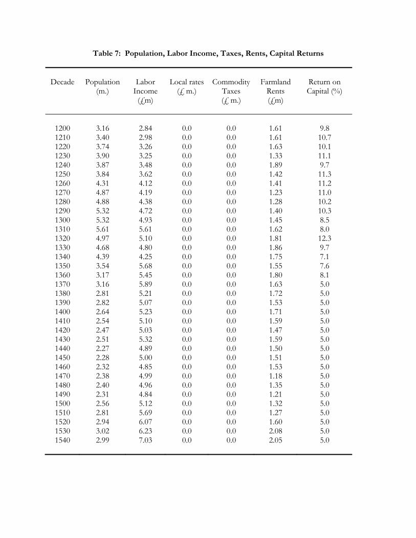
Table 7: Population, Labor Income, Taxes, Rents, Capital Returns
Decade
Population
(m.)
Labor
Income (£m)
Local rates
(£ m.)
Commodity
Taxes (£ m.)
Farmland
Rents (£m)
Return on Capital (%)
1200 3.16 2.84 0.0 0.0 1.61 9.8 1210 3.40 2.98 0.0 0.0 1.61 10.7 1220 3.74 3.26 0.0 0.0 1.63 10.1 1230 3.90 3.25 0.0 0.0 1.33 11.1 1240 3.87 3.48 0.0 0.0 1.89 9.7 1250 3.84 3.62 0.0 0.0 1.42 11.3 1260 4.31 4.12 0.0 0.0 1.41 11.2 1270 4.87 4.19 0.0 0.0 1.23 11.0 1280 4.88 4.38 0.0 0.0 1.28 10.2 1290 5.32 4.72 0.0 0.0 1.40 10.3 1300 5.32 4.93 0.0 0.0 1.45 8.5 1310 5.61 5.61 0.0 0.0 1.62 8.0 1320 4.97 5.10 0.0 0.0 1.81 12.3 1330 4.68 4.80 0.0 0.0 1.86 9.7 1340 4.39 4.25 0.0 0.0 1.75 7.1 1350 3.54 5.68 0.0 0.0 1.55 7.6 1360 3.17 5.45 0.0 0.0 1.80 8.1 1370 3.16 5.89 0.0 0.0 1.63 5.0 1380 2.81 5.21 0.0 0.0 1.72 5.0 1390 2.82 5.07 0.0 0.0 1.53 5.0 1400 2.64 5.23 0.0 0.0 1.71 5.0 1410 2.54 5.10 0.0 0.0 1.59 5.0 1420 2.47 5.03 0.0 0.0 1.47 5.0 1430 2.51 5.32 0.0 0.0 1.59 5.0 1440 2.27 4.89 0.0 0.0 1.50 5.0 1450 2.28 5.00 0.0 0.0 1.51 5.0 1460 2.32 4.85 0.0 0.0 1.53 5.0 1470 2.38 4.99 0.0 0.0 1.18 5.0 1480 2.40 4.96 0.0 0.0 1.35 5.0 1490 2.31 4.84 0.0 0.0 1.21 5.0 1500 2.56 5.12 0.0 0.0 1.32 5.0 1510 2.81 5.69 0.0 0.0 1.27 5.0 1520 2.94 6.07 0.0 0.0 1.60 5.0 1530 3.02 6.23 0.0 0.0 2.08 5.0 1540 2.99 7.03 0.0 0.0 2.05 5.0
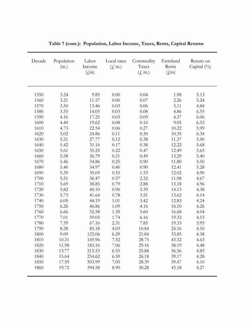
Table 7 (cont.): Population, Labor Income, Taxes, Rents, Capital Returns
Decade
Population
(m.)
Labor
Income (£m)
Local rates
(£ m.)
Commodity
Taxes (£ m.)
Farmland
Rents (£m)
Return on Capital (%)
1550 3.24 9.85 0.00 0.04 1.98 5.13 1560 3.21 11.57 0.00 0.07 2.26 5.24 1570 3.50 13.46 0.03 0.06 3.11 4.84 1580 3.55 14.05 0.03 0.08 4.86 6.55 1590 4.16 17.25 0.03 0.09 4.37 6.06 1600 4.40 19.62 0.08 0.16 9.05 6.52 1610 4.73 22.54 0.06 0.27 10.22 5.99 1620 5.02 24.86 0.11 0.30 10.35 6.34 1630 5.21 27.77 0.12 0.38 11.37 5.90 1640 5.42 31.16 0.17 0.38 12.22 5.68 1650 5.61 35.25 0.22 0.47 12.49 5.63 1660 5.58 36.79 0.21 0.49 13.29 5.40 1670 5.46 34.86 0.25 0.90 11.80 5.50 1680 5.40 34.97 0.40 0.90 12.41 5.28 1690 5.39 35.05 0.55 1.53 12.02 4.90 1700 5.51 36.47 0.57 2.32 11.98 4.67 1710 5.69 38.85 0.79 2.88 13.18 4.96 1720 5.82 40.10 0.90 3.39 14.13 4.38 1730 5.73 41.64 0.78 3.51 13.62 4.14 1740 6.05 44.19 1.01 3.42 12.83 4.24 1750 6.26 46.86 1.09 4.16 16.10 4.26 1760 6.66 52.58 1.39 5.60 16.68 4.04 1770 7.01 59.05 1.74 6.16 19.32 4.15 1780 7.59 67.16 2.31 7.85 19.33 3.95 1790 8.28 85.18 4.03 10.84 24.16 4.10 1800 9.09 123.06 6.29 21.84 33.85 4.38 1810 10.31 169.96 7.52 28.75 43.32 4.63 1820 11.98 183.16 7.06 29.16 38.19 4.48 1830 13.77 215.53 6.55 25.88 36.56 4.85 1840 15.64 254.62 6.59 26.18 39.17 4.28 1850 17.59 303.99 7.05 28.39 39.47 4.10 1860 19.72 394.58 8.90 30.28 43.18 4.27
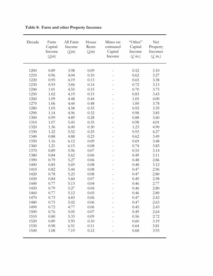
Table 8: Farm and other Property Incomes
Decade
Farm
Capital Income
(£m)
All Farm Income
(£m)
House Rents (£m)
Mines etc estimated Capital Income
“Other” Capital Income (£ m.)
Net
Property Incomes (£ m.)
1200 0.89 3.98 0.09 - 0.52 3.10 1210 0.96 4.04 0.10 - 0.62 3.27 1220 0.95 4.19 0.13 - 0.65 3.38 1230 0.93 3.84 0.14 - 0.72 3.13 1240 1.01 4.55 0.15 - 0.70 3.75 1250 1.02 4.19 0.15 - 0.83 3.43 1260 1.09 4.48 0.44 - 1.05 4.00 1270 1.06 4.44 0.48 - 1.00 3.78 1280 1.05 4.58 0.35 - 0.92 3.59 1290 1.14 4.96 0.32 - 0.98 3.85 1300 0.99 4.89 0.28 - 0.88 3.60 1310 1.07 5.45 0.35 - 0.98 4.01 1320 1.56 6.00 0.30 - 1.23 4.90 1330 1.22 5.52 0.25 - 0.93 4.27 1340 0.88 4.88 0.23 - 0.62 3.49 1350 1.16 6.12 0.09 - 0.69 3.48 1360 1.21 6.15 0.08 - 0.74 3.83 1370 0.89 5.96 0.07 - 0.55 3.14 1380 0.84 5.62 0.06 - 0.49 3.11 1390 0.79 5.27 0.06 - 0.48 2.86 1400 0.85 5.69 0.08 - 0.48 3.12 1410 0.82 5.44 0.08 - 0.47 2.96 1420 0.78 5.23 0.08 - 0.47 2.80 1430 0.84 5.60 0.07 - 0.49 2.98 1440 0.77 5.13 0.04 - 0.46 2.77 1450 0.79 5.27 0.04 - 0.46 2.80 1460 0.77 5.12 0.05 - 0.46 2.80 1470 0.73 4.83 0.06 - 0.47 2.43 1480 0.75 5.02 0.06 - 0.47 2.63 1490 0.72 4.77 0.06 - 0.45 2.43 1500 0.76 5.05 0.07 - 0.49 2.64 1510 0.80 5.33 0.09 - 0.56 2.72 1520 0.89 5.95 0.10 - 0.60 3.19 1530 0.98 6.51 0.11 - 0.64 3.81 1540 1.08 7.19 0.12 - 0.68 3.93
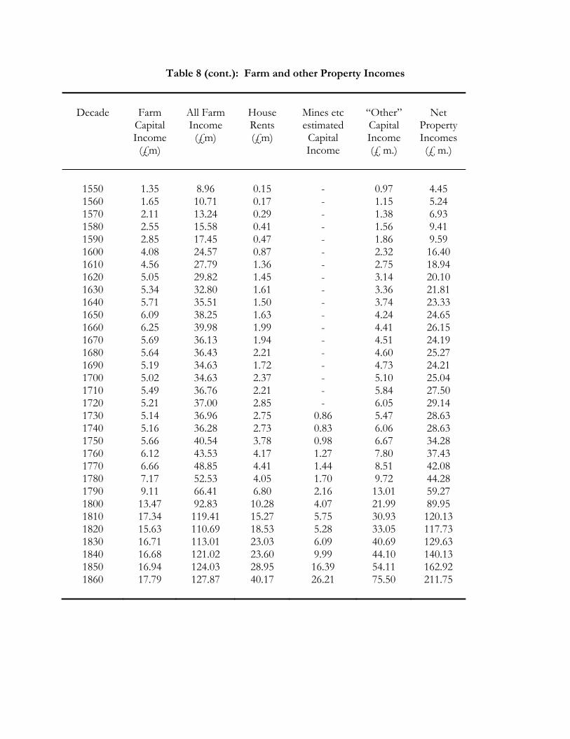
Table 8 (cont.): Farm and other Property Incomes
Decade
Farm
Capital Income
(£m)
All Farm Income
(£m)
House Rents (£m)
Mines etc estimated Capital Income
“Other” Capital Income (£ m.)
Net
Property Incomes (£ m.)
1550 1.35 8.96 0.15 - 0.97 4.45 1560 1.65 10.71 0.17 - 1.15 5.24 1570 2.11 13.24 0.29 - 1.38 6.93 1580 2.55 15.58 0.41 - 1.56 9.41 1590 2.85 17.45 0.47 - 1.86 9.59 1600 4.08 24.57 0.87 - 2.32 16.40 1610 4.56 27.79 1.36 - 2.75 18.94 1620 5.05 29.82 1.45 - 3.14 20.10 1630 5.34 32.80 1.61 - 3.36 21.81 1640 5.71 35.51 1.50 - 3.74 23.33 1650 6.09 38.25 1.63 - 4.24 24.65 1660 6.25 39.98 1.99 - 4.41 26.15 1670 5.69 36.13 1.94 - 4.51 24.19 1680 5.64 36.43 2.21 - 4.60 25.27 1690 5.19 34.63 1.72 - 4.73 24.21 1700 5.02 34.63 2.37 - 5.10 25.04 1710 5.49 36.76 2.21 - 5.84 27.50 1720 5.21 37.00 2.85 - 6.05 29.14 1730 5.14 36.96 2.75 0.86 5.47 28.63 1740 5.16 36.28 2.73 0.83 6.06 28.63 1750 5.66 40.54 3.78 0.98 6.67 34.28 1760 6.12 43.53 4.17 1.27 7.80 37.43 1770 6.66 48.85 4.41 1.44 8.51 42.08 1780 7.17 52.53 4.05 1.70 9.72 44.28 1790 9.11 66.41 6.80 2.16 13.01 59.27 1800 13.47 92.83 10.28 4.07 21.99 89.95 1810 17.34 119.41 15.27 5.75 30.93 120.13 1820 15.63 110.69 18.53 5.28 33.05 117.73 1830 16.71 113.01 23.03 6.09 40.69 129.63 1840 16.68 121.02 23.60 9.99 44.10 140.13 1850 16.94 124.03 28.95 16.39 54.11 162.92 1860 17.79 127.87 40.17 26.21 75.50 211.75
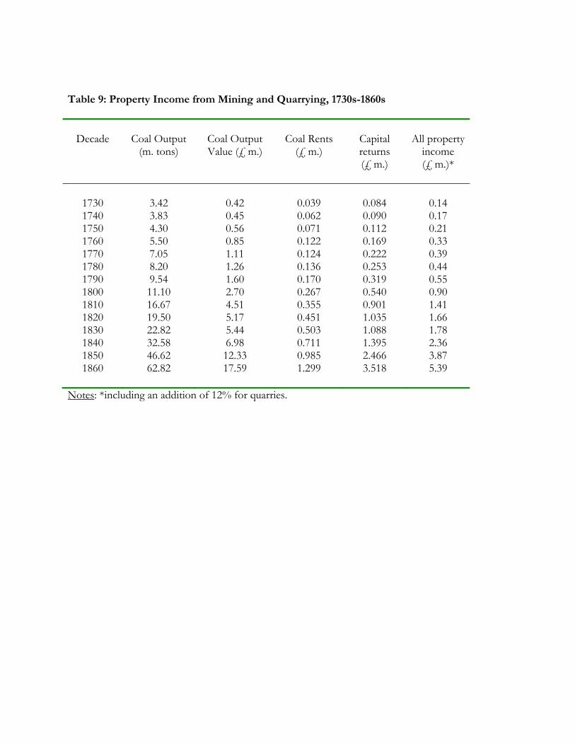
Table 9: Property Income from Mining and Quarrying, 1730s-1860s
Decade
Coal Output
(m. tons)
Coal Output Value (£ m.)
Coal Rents
(£ m.)
Capital returns (£ m.)
All property
income (£ m.)*
1730 3.42 0.42 0.039 0.084 0.14 1740 3.83 0.45 0.062 0.090 0.17 1750 4.30 0.56 0.071 0.112 0.21 1760 5.50 0.85 0.122 0.169 0.33 1770 7.05 1.11 0.124 0.222 0.39 1780 8.20 1.26 0.136 0.253 0.44 1790 9.54 1.60 0.170 0.319 0.55 1800 11.10 2.70 0.267 0.540 0.90 1810 16.67 4.51 0.355 0.901 1.41 1820 19.50 5.17 0.451 1.035 1.66 1830 22.82 5.44 0.503 1.088 1.78 1840 32.58 6.98 0.711 1.395 2.36 1850 46.62 12.33 0.985 2.466 3.87 1860 62.82 17.59 1.299 3.518 5.39
Notes: *including an addition of 12% for quarries.
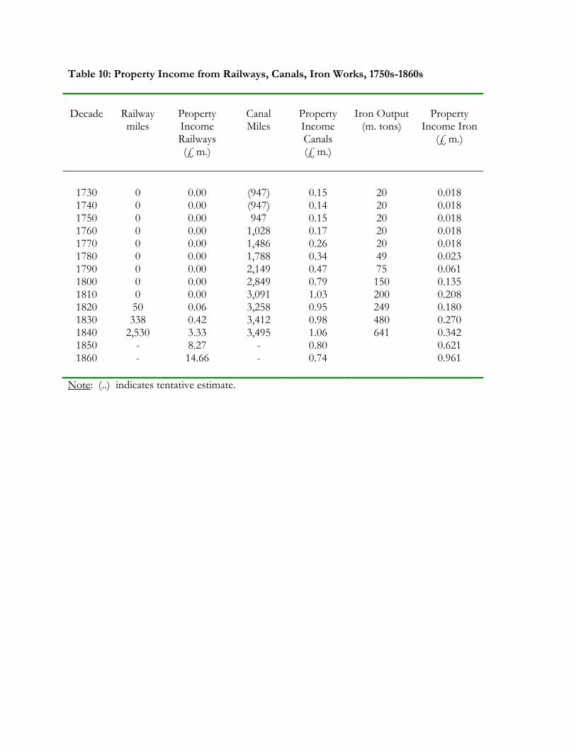
Table 10: Property Income from Railways, Canals, Iron Works, 1750s-1860s
Decade
Railway miles
Property Income Railways (£ m.)
Canal Miles
Property Income Canals (£ m.)
Iron Output
(m. tons)
Property
Income Iron (£ m.)
1730 0 0.00 (947) 0.15 20 0.018 1740 0 0.00 (947) 0.14 20 0.018 1750 0 0.00 947 0.15 20 0.018 1760 0 0.00 1,028 0.17 20 0.018 1770 0 0.00 1,486 0.26 20 0.018 1780 0 0.00 1,788 0.34 49 0.023 1790 0 0.00 2,149 0.47 75 0.061 1800 0 0.00 2,849 0.79 150 0.135 1810 0 0.00 3,091 1.03 200 0.208 1820 50 0.06 3,258 0.95 249 0.180 1830 338 0.42 3,412 0.98 480 0.270 1840 2,530 3.33 3,495 1.06 641 0.342 1850 - 8.27 - 0.80 0.621 1860 - 14.66 - 0.74 0.961
Note: (..) indicates tentative estimate.
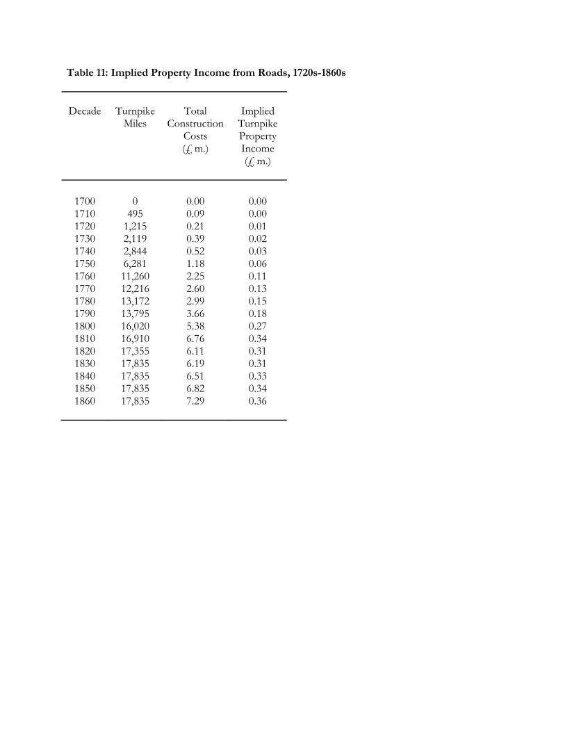
Table 11: Implied Property Income from Roads, 1720s-1860s
Decade
Turnpike
Miles
Total
Construction Costs (£ m.)
Implied
Turnpike Property Income (£ m.)
1700 0 0.00 0.00 1710 495 0.09 0.00 1720 1,215 0.21 0.01 1730 2,119 0.39 0.02 1740 2,844 0.52 0.03 1750 6,281 1.18 0.06 1760 11,260 2.25 0.11 1770 12,216 2.60 0.13 1780 13,172 2.99 0.15 1790 13,795 3.66 0.18 1800 16,020 5.38 0.27 1810 16,910 6.76 0.34 1820 17,355 6.11 0.31 1830 17,835 6.19 0.31 1840 17,835 6.51 0.33 1850 17,835 6.82 0.34 1860 17,835 7.29 0.36
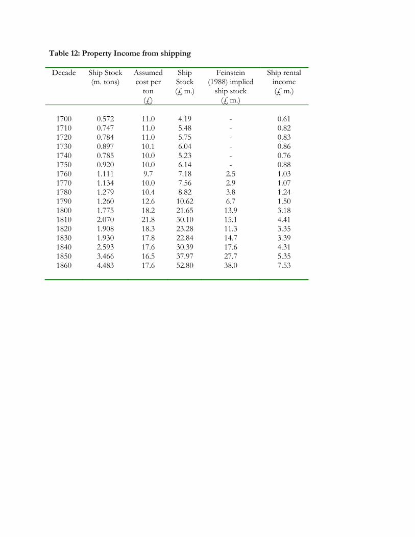
Table 12: Property Income from shipping Decade Ship Stock
(m. tons) Assumed cost per
ton (£)
Ship Stock (£ m.)
Feinstein (1988) implied
ship stock (£ m.)
Ship rental income (£ m.)
1700 0.572 11.0 4.19 - 0.61 1710 0.747 11.0 5.48 - 0.82 1720 0.784 11.0 5.75 - 0.83 1730 0.897 10.1 6.04 - 0.86 1740 0.785 10.0 5.23 - 0.76 1750 0.920 10.0 6.14 - 0.88 1760 1.111 9.7 7.18 2.5 1.03 1770 1.134 10.0 7.56 2.9 1.07 1780 1.279 10.4 8.82 3.8 1.24 1790 1.260 12.6 10.62 6.7 1.50 1800 1.775 18.2 21.65 13.9 3.18 1810 2.070 21.8 30.10 15.1 4.41 1820 1.908 18.3 23.28 11.3 3.35 1830 1.930 17.8 22.84 14.7 3.39 1840 2.593 17.6 30.39 17.6 4.31 1850 3.466 16.5 37.97 27.7 5.35 1860 4.483 17.6 52.80 38.0 7.53
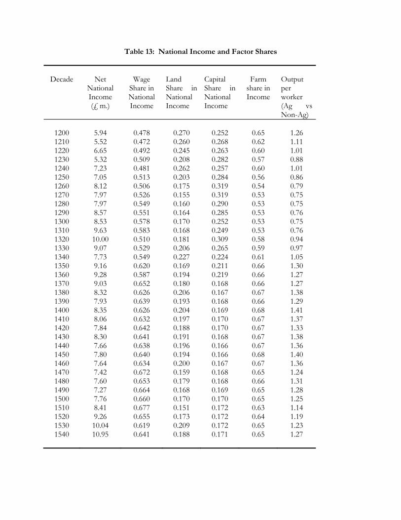
Table 13: National Income and Factor Shares
Decade
Net
National Income (£ m.)
Wage
Share in National Income
Land Share in National Income
Capital Share in National Income
Farm
share in Income
Output per worker (Ag vs Non-Ag)
1200 5.94 0.478 0.270 0.252 0.65 1.26 1210 5.52 0.472 0.260 0.268 0.62 1.11 1220 6.65 0.492 0.245 0.263 0.60 1.01 1230 5.32 0.509 0.208 0.282 0.57 0.88 1240 7.23 0.481 0.262 0.257 0.60 1.01 1250 7.05 0.513 0.203 0.284 0.56 0.86 1260 8.12 0.506 0.175 0.319 0.54 0.79 1270 7.97 0.526 0.155 0.319 0.53 0.75 1280 7.97 0.549 0.160 0.290 0.53 0.75 1290 8.57 0.551 0.164 0.285 0.53 0.76 1300 8.53 0.578 0.170 0.252 0.53 0.75 1310 9.63 0.583 0.168 0.249 0.53 0.76 1320 10.00 0.510 0.181 0.309 0.58 0.94 1330 9.07 0.529 0.206 0.265 0.59 0.97 1340 7.73 0.549 0.227 0.224 0.61 1.05 1350 9.16 0.620 0.169 0.211 0.66 1.30 1360 9.28 0.587 0.194 0.219 0.66 1.27 1370 9.03 0.652 0.180 0.168 0.66 1.27 1380 8.32 0.626 0.206 0.167 0.67 1.38 1390 7.93 0.639 0.193 0.168 0.66 1.29 1400 8.35 0.626 0.204 0.169 0.68 1.41 1410 8.06 0.632 0.197 0.170 0.67 1.37 1420 7.84 0.642 0.188 0.170 0.67 1.33 1430 8.30 0.641 0.191 0.168 0.67 1.38 1440 7.66 0.638 0.196 0.166 0.67 1.36 1450 7.80 0.640 0.194 0.166 0.68 1.40 1460 7.64 0.634 0.200 0.167 0.67 1.36 1470 7.42 0.672 0.159 0.168 0.65 1.24 1480 7.60 0.653 0.179 0.168 0.66 1.31 1490 7.27 0.664 0.168 0.169 0.65 1.28 1500 7.76 0.660 0.170 0.170 0.65 1.25 1510 8.41 0.677 0.151 0.172 0.63 1.14 1520 9.26 0.655 0.173 0.172 0.64 1.19 1530 10.04 0.619 0.209 0.172 0.65 1.23 1540 10.95 0.641 0.188 0.171 0.65 1.27
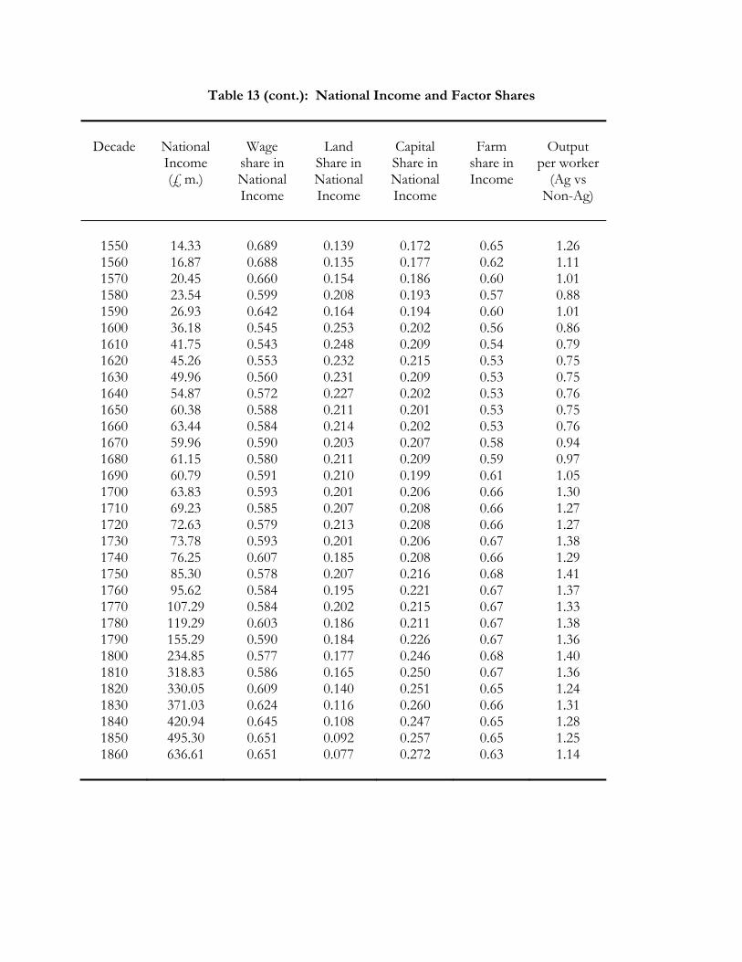
Table 13 (cont.): National Income and Factor Shares
Decade
National Income (£ m.)
Wage
share in National Income
Land
Share in National Income
Capital Share in National Income
Farm
share in Income
Output
per worker (Ag vs
Non-Ag)
1550 14.33 0.689 0.139 0.172 0.65 1.26 1560 16.87 0.688 0.135 0.177 0.62 1.11 1570 20.45 0.660 0.154 0.186 0.60 1.01 1580 23.54 0.599 0.208 0.193 0.57 0.88 1590 26.93 0.642 0.164 0.194 0.60 1.01 1600 36.18 0.545 0.253 0.202 0.56 0.86 1610 41.75 0.543 0.248 0.209 0.54 0.79 1620 45.26 0.553 0.232 0.215 0.53 0.75 1630 49.96 0.560 0.231 0.209 0.53 0.75 1640 54.87 0.572 0.227 0.202 0.53 0.76 1650 60.38 0.588 0.211 0.201 0.53 0.75 1660 63.44 0.584 0.214 0.202 0.53 0.76 1670 59.96 0.590 0.203 0.207 0.58 0.94 1680 61.15 0.580 0.211 0.209 0.59 0.97 1690 60.79 0.591 0.210 0.199 0.61 1.05 1700 63.83 0.593 0.201 0.206 0.66 1.30 1710 69.23 0.585 0.207 0.208 0.66 1.27 1720 72.63 0.579 0.213 0.208 0.66 1.27 1730 73.78 0.593 0.201 0.206 0.67 1.38 1740 76.25 0.607 0.185 0.208 0.66 1.29 1750 85.30 0.578 0.207 0.216 0.68 1.41 1760 95.62 0.584 0.195 0.221 0.67 1.37 1770 107.29 0.584 0.202 0.215 0.67 1.33 1780 119.29 0.603 0.186 0.211 0.67 1.38 1790 155.29 0.590 0.184 0.226 0.67 1.36 1800 234.85 0.577 0.177 0.246 0.68 1.40 1810 318.83 0.586 0.165 0.250 0.67 1.36 1820 330.05 0.609 0.140 0.251 0.65 1.24 1830 371.03 0.624 0.116 0.260 0.66 1.31 1840 420.94 0.645 0.108 0.247 0.65 1.28 1850 495.30 0.651 0.092 0.257 0.65 1.25 1860 636.61 0.651 0.077 0.272 0.63 1.14
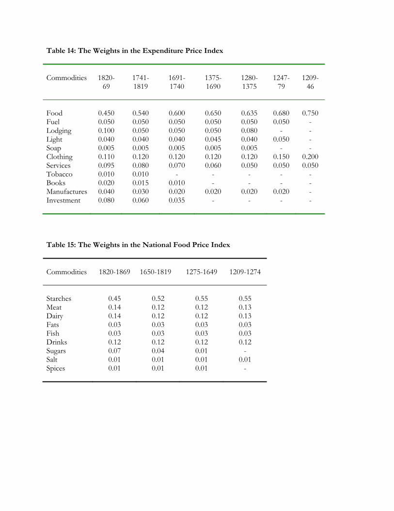
Table 14: The Weights in the Expenditure Price Index
Commodities
1820-
69
1741-1819
1691-1740
1375-1690
1280-1375
1247-
79
1209-
46
Food 0.450 0.540 0.600 0.650 0.635 0.680 0.750 Fuel 0.050 0.050 0.050 0.050 0.050 0.050 - Lodging 0.100 0.050 0.050 0.050 0.080 - - Light 0.040 0.040 0.040 0.045 0.040 0.050 - Soap 0.005 0.005 0.005 0.005 0.005 - - Clothing 0.110 0.120 0.120 0.120 0.120 0.150 0.200 Services 0.095 0.080 0.070 0.060 0.050 0.050 0.050 Tobacco 0.010 0.010 - - - - - Books 0.020 0.015 0.010 - - - - Manufactures 0.040 0.030 0.020 0.020 0.020 0.020 - Investment 0.080 0.060 0.035 - - - -
Table 15: The Weights in the National Food Price Index
Commodities
1820-1869
1650-1819
1275-1649
1209-1274
Starches 0.45 0.52 0.55 0.55 Meat 0.14 0.12 0.12 0.13 Dairy 0.14 0.12 0.12 0.13 Fats 0.03 0.03 0.03 0.03 Fish 0.03 0.03 0.03 0.03 Drinks 0.12 0.12 0.12 0.12 Sugars 0.07 0.04 0.01 - Salt 0.01 0.01 0.01 0.01 Spices 0.01 0.01 0.01 -
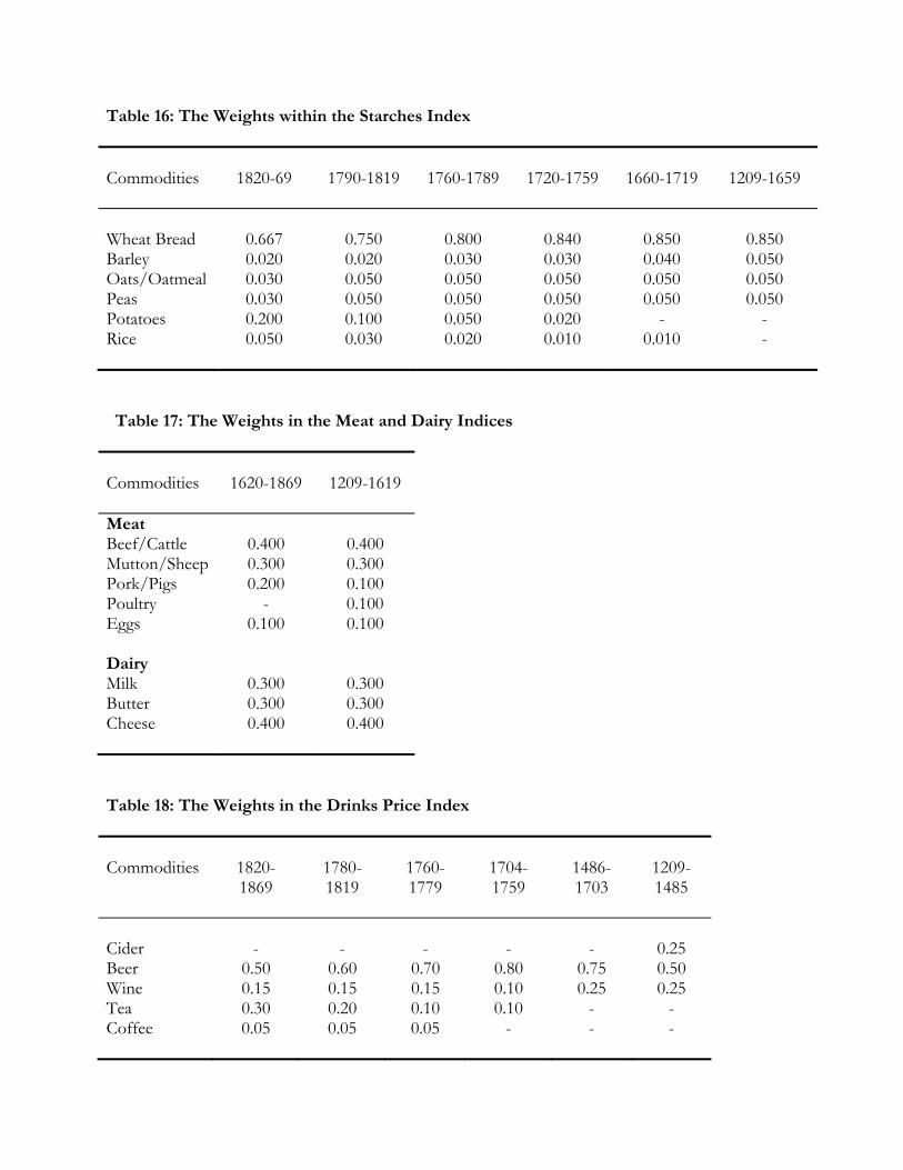
Table 16: The Weights within the Starches Index
Commodities
1820-69
1790-1819
1760-1789
1720-1759
1660-1719
1209-1659
Wheat Bread 0.667 0.750 0.800 0.840 0.850 0.850 Barley 0.020 0.020 0.030 0.030 0.040 0.050 Oats/Oatmeal 0.030 0.050 0.050 0.050 0.050 0.050 Peas 0.030 0.050 0.050 0.050 0.050 0.050 Potatoes 0.200 0.100 0.050 0.020 - - Rice 0.050 0.030 0.020 0.010 0.010 -
Table 17: The Weights in the Meat and Dairy Indices
Commodities
1620-1869
1209-1619
Meat Beef/Cattle 0.400 0.400 Mutton/Sheep 0.300 0.300 Pork/Pigs 0.200 0.100 Poultry - 0.100 Eggs 0.100 0.100 Dairy Milk 0.300 0.300 Butter 0.300 0.300 Cheese 0.400 0.400
Table 18: The Weights in the Drinks Price Index
Commodities
1820-1869
1780-1819
1760-1779
1704-1759
1486-1703
1209-1485
Cider - - - - - 0.25 Beer 0.50 0.60 0.70 0.80 0.75 0.50 Wine 0.15 0.15 0.15 0.10 0.25 0.25 Tea 0.30 0.20 0.10 0.10 - - Coffee 0.05 0.05 0.05 - - -
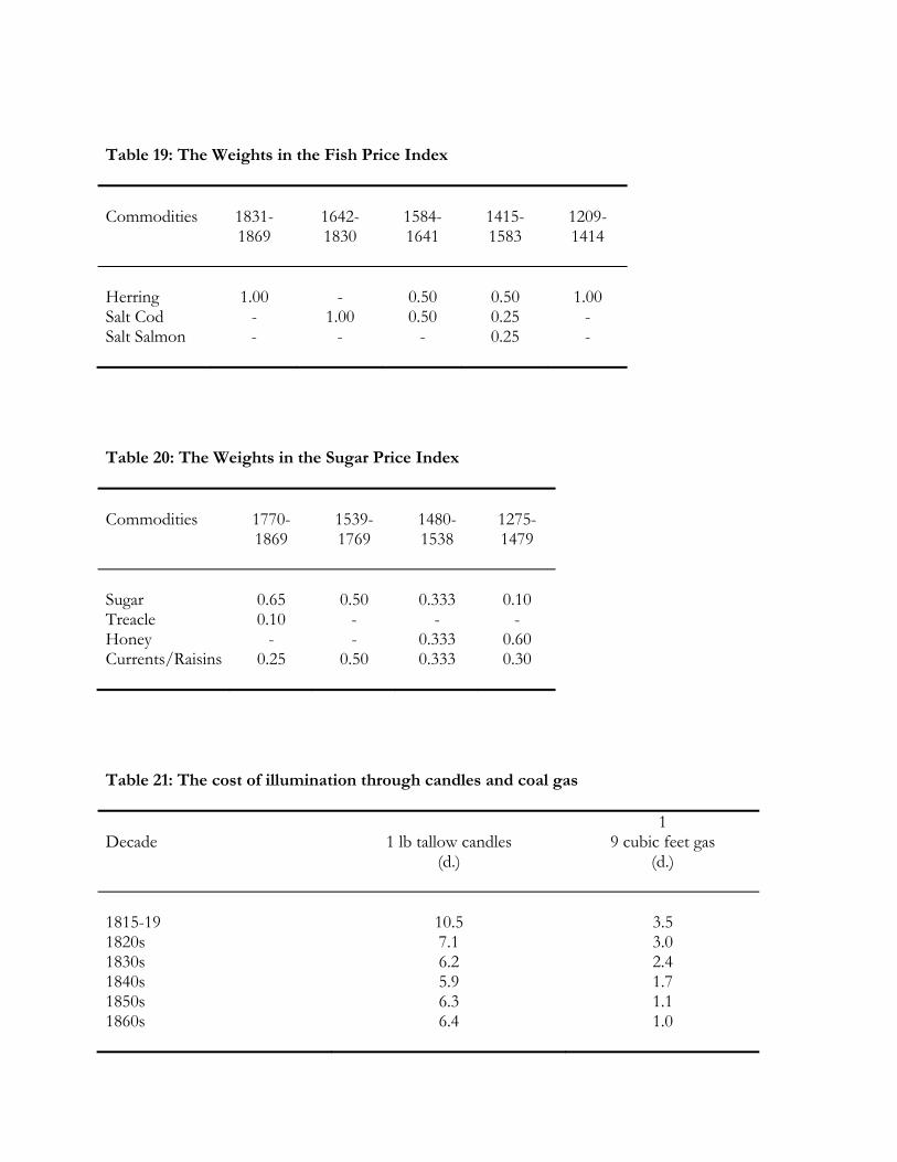
Table 19: The Weights in the Fish Price Index
Commodities
1831-1869
1642-1830
1584-1641
1415-1583
1209-1414
Herring 1.00 - 0.50 0.50 1.00 Salt Cod - 1.00 0.50 0.25 - Salt Salmon - - - 0.25 -
Table 20: The Weights in the Sugar Price Index
Commodities
1770-1869
1539-1769
1480-1538
1275-1479
Sugar 0.65 0.50 0.333 0.10 Treacle 0.10 - - - Honey - - 0.333 0.60 Currents/Raisins 0.25 0.50 0.333 0.30
Table 21: The cost of illumination through candles and coal gas
Decade
1 lb tallow candles
(d.)
1 9 cubic feet gas
(d.)
1815-19 10.5 3.5 1820s 7.1 3.0 1830s 6.2 2.4 1840s 5.9 1.7 1850s 6.3 1.1 1860s 6.4 1.0
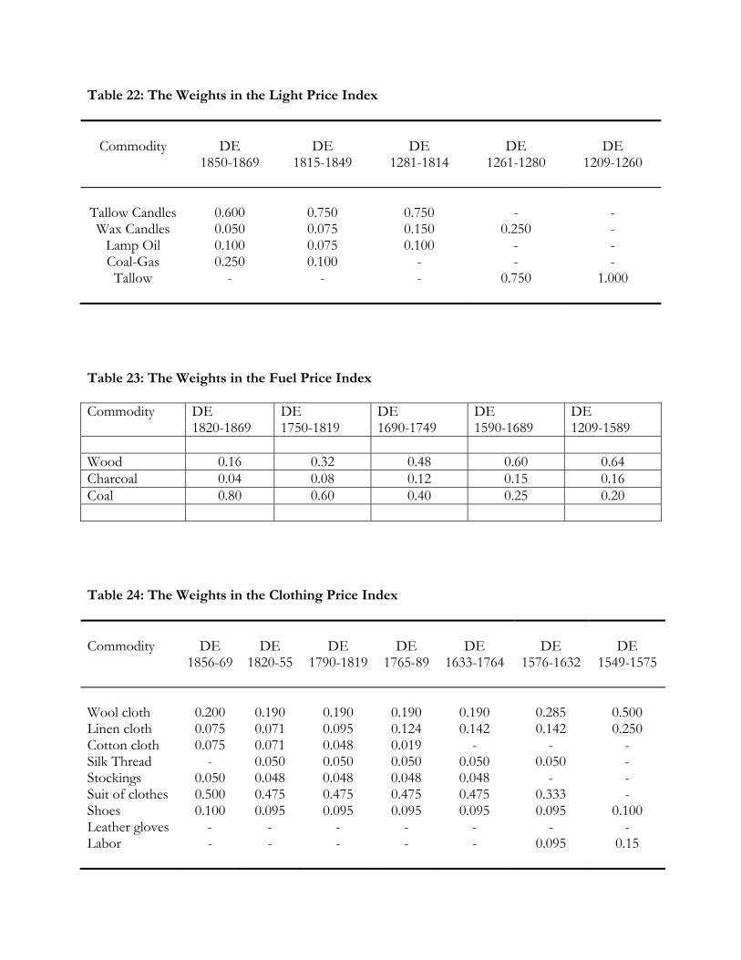
Table 22: The Weights in the Light Price Index
Commodity
DE
1850-1869
DE
1815-1849
DE
1281-1814
DE
1261-1280
DE
1209-1260
Tallow Candles 0.600 0.750 0.750 - - Wax Candles 0.050 0.075 0.150 0.250 -
Lamp Oil 0.100 0.075 0.100 - - Coal-Gas 0.250 0.100 - - - Tallow - - - 0.750 1.000
Table 23: The Weights in the Fuel Price Index
Commodity DE 1820-1869
DE 1750-1819
DE 1690-1749
DE 1590-1689
DE 1209-1589
Wood 0.16 0.32 0.48 0.60 0.64 Charcoal 0.04 0.08 0.12 0.15 0.16 Coal 0.80 0.60 0.40 0.25 0.20
Table 24: The Weights in the Clothing Price Index
Commodity
DE
1856-69
DE
1820-55
DE
1790-1819
DE
1765-89
DE
1633-1764
DE
1576-1632
DE
1549-1575
Wool cloth 0.200 0.190 0.190 0.190 0.190 0.285 0.500 Linen cloth 0.075 0.071 0.095 0.124 0.142 0.142 0.250 Cotton cloth 0.075 0.071 0.048 0.019 - - - Silk Thread - 0.050 0.050 0.050 0.050 0.050 - Stockings 0.050 0.048 0.048 0.048 0.048 - - Suit of clothes 0.500 0.475 0.475 0.475 0.475 0.333 - Shoes 0.100 0.095 0.095 0.095 0.095 0.095 0.100 Leather gloves - - - - - - - Labor - - - - - 0.095 0.15
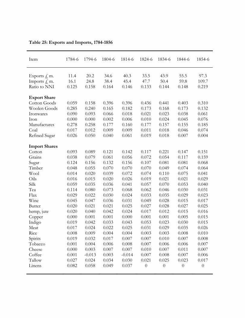
Table 25: Exports and Imports, 1784-1856 Item
1784-6
1794-6
1804-6
1814-6
1824-6
1834-6
1844-6
1854-6
Exports £ m. 11.4 20.2 34.6 40.3 33.5 43.9 55.5 97.3 Imports £ m. 16.1 24.8 38.4 45.4 47.7 50.4 59.8 109.7 Ratio to NNI 0.125 0.158 0.164 0.146 0.133 0.144 0.148 0.219 Export Share Cotton Goods 0.059 0.158 0.396 0.396 0.436 0.441 0.403 0.310 Woolen Goods 0.285 0.240 0.165 0.182 0.173 0.168 0.173 0.132 Ironwares 0.090 0.093 0.066 0.018 0.021 0.023 0.038 0.061 Iron 0.000 0.000 0.002 0.006 0.010 0.024 0.045 0.076 Manufactures 0.278 0.258 0.177 0.160 0.177 0.157 0.155 0.185 Coal 0.017 0.012 0.009 0.009 0.011 0.018 0.046 0.074 Refined Sugar 0.026 0.050 0.040 0.061 0.019 0.018 0.007 0.004 Import Shares Cotton 0.093 0.089 0.121 0.142 0.117 0.221 0.147 0.151 Grains 0.038 0.079 0.061 0.056 0.072 0.054 0.117 0.159 Sugar 0.124 0.156 0.132 0.156 0.107 0.081 0.081 0.068 Timber 0.048 0.055 0.070 0.070 0.070 0.049 0.074 0.064 Wool 0.014 0.020 0.039 0.072 0.074 0.110 0.075 0.041 Oils 0.016 0.015 0.020 0.026 0.019 0.021 0.021 0.029 Silk 0.059 0.035 0.036 0.041 0.057 0.070 0.053 0.040 Tea 0.114 0.080 0.073 0.068 0.062 0.046 0.030 0.031 Flax 0.029 0.022 0.030 0.024 0.033 0.035 0.029 0.023 Wine 0.045 0.047 0.036 0.031 0.049 0.028 0.015 0.017 Butter 0.020 0.021 0.021 0.025 0.027 0.028 0.027 0.025 hemp, jute 0.020 0.040 0.042 0.024 0.017 0.012 0.015 0.016 Copper 0.000 0.001 0.001 0.000 0.001 0.001 0.005 0.015 Indigo 0.019 0.042 0.033 0.043 0.053 0.023 0.030 0.015 Meat 0.017 0.024 0.022 0.025 0.031 0.029 0.035 0.026 Rice 0.008 0.009 0.004 0.004 0.003 0.003 0.008 0.010 Spirits 0.019 0.032 0.017 0.007 0.007 0.010 0.007 0.008 Tobacco 0.001 0.004 0.006 0.008 0.007 0.006 0.006 0.007 Cheese 0.000 0.003 0.007 0.007 0.010 0.007 0.011 0.007 Coffee 0.001 -0.013 0.003 -0.014 0.007 0.008 0.007 0.006 Tallow 0.027 0.024 0.034 0.030 0.021 0.025 0.023 0.017 Linens 0.082 0.058 0.049 0.037 0 0 0 0

Table 26: Exports and Imports, 1699-1774
Item
1699-1701
1722-4
1752-4
1772-4
Exports £ m. 4.43 5.04 8.42 9.85 Imports £ m. 3.86 4.04 4.71 6.92 Ratio to NNI 0.072 0.066 0.086 0.088 Export Shares Cotton Goods 0.000 0.000 0.000 0.022 Woolen Goods 0.687 0.592 0.467 0.425 Ironwares 0.026 0.036 0.070 0.122 Manufactures 0.063 0.074 0.134 0.187 Coal 0.008 0.019 0.021 0.034 Grains 0.033 0.117 0.107 0.004 Import Shares Cotton - - - 0.020 Grains 0.000 0.000 0.000 0.043 Sugar 0.089 0.177 0.185 0.280 Timber 0.036 0.039 0.050 0.046 Wool 0.052 0.028 0.016 0.015 Silk 0.073 0.162 0.133 0.091 Tea 0.000 0.000 0.117 0.080 Wine 0.139 0.142 0.087 0.059 Tallow 0.022 0.004 0.001 0.019 Linens 0.187 0.193 0.136 0.022
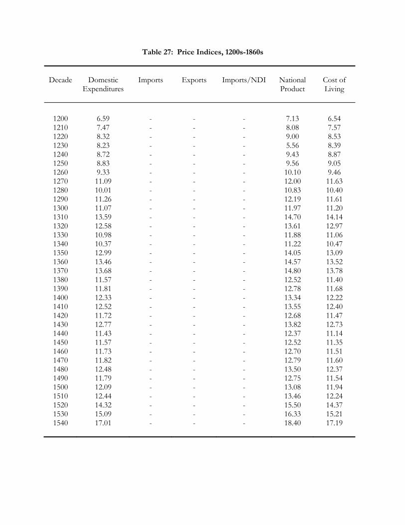
Table 27: Price Indices, 1200s-1860s
Decade
Domestic
Expenditures
Imports
Exports
Imports/NDI
National Product
Cost of Living
1200 6.59 - - - 7.13 6.54 1210 7.47 - - - 8.08 7.57 1220 8.32 - - - 9.00 8.53 1230 8.23 - - - 5.56 8.39 1240 8.72 - - - 9.43 8.87 1250 8.83 - - - 9.56 9.05 1260 9.33 - - - 10.10 9.46 1270 11.09 - - - 12.00 11.63 1280 10.01 - - - 10.83 10.40 1290 11.26 - - - 12.19 11.61 1300 11.07 - - - 11.97 11.20 1310 13.59 - - - 14.70 14.14 1320 12.58 - - - 13.61 12.97 1330 10.98 - - - 11.88 11.06 1340 10.37 - - - 11.22 10.47 1350 12.99 - - - 14.05 13.09 1360 13.46 - - - 14.57 13.52 1370 13.68 - - - 14.80 13.78 1380 11.57 - - - 12.52 11.40 1390 11.81 - - - 12.78 11.68 1400 12.33 - - - 13.34 12.22 1410 12.52 - - - 13.55 12.40 1420 11.72 - - - 12.68 11.47 1430 12.77 - - - 13.82 12.73 1440 11.43 - - - 12.37 11.14 1450 11.57 - - - 12.52 11.35 1460 11.73 - - - 12.70 11.51 1470 11.82 - - - 12.79 11.60 1480 12.48 - - - 13.50 12.37 1490 11.79 - - - 12.75 11.54 1500 12.09 - - - 13.08 11.94 1510 12.44 - - - 13.46 12.24 1520 14.32 - - - 15.50 14.37 1530 15.09 - - - 16.33 15.21 1540 17.01 - - - 18.40 17.19
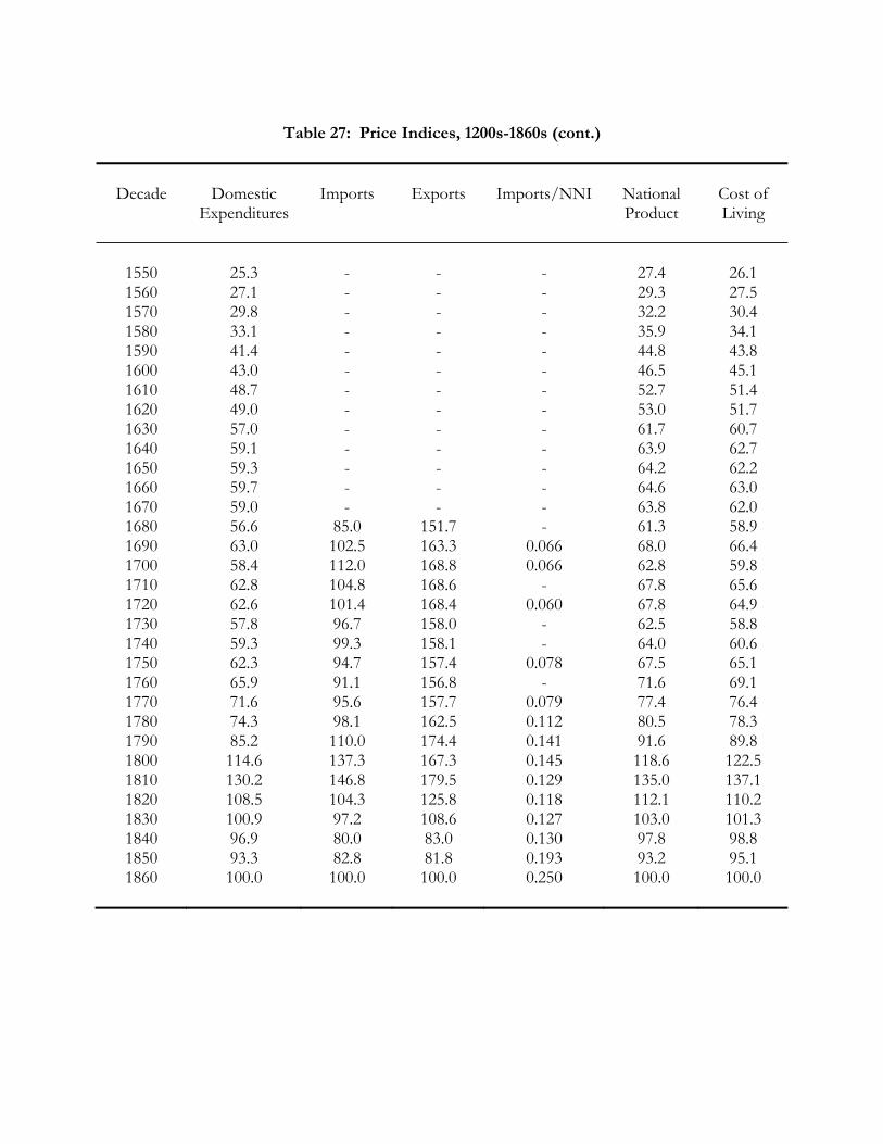
Table 27: Price Indices, 1200s-1860s (cont.)
Decade
Domestic
Expenditures
Imports
Exports
Imports/NNI
National Product
Cost of Living
1550 25.3 - - - 27.4 26.1 1560 27.1 - - - 29.3 27.5 1570 29.8 - - - 32.2 30.4 1580 33.1 - - - 35.9 34.1 1590 41.4 - - - 44.8 43.8 1600 43.0 - - - 46.5 45.1 1610 48.7 - - - 52.7 51.4 1620 49.0 - - - 53.0 51.7 1630 57.0 - - - 61.7 60.7 1640 59.1 - - - 63.9 62.7 1650 59.3 - - - 64.2 62.2 1660 59.7 - - - 64.6 63.0 1670 59.0 - - - 63.8 62.0 1680 56.6 85.0 151.7 - 61.3 58.9 1690 63.0 102.5 163.3 0.066 68.0 66.4 1700 58.4 112.0 168.8 0.066 62.8 59.8 1710 62.8 104.8 168.6 - 67.8 65.6 1720 62.6 101.4 168.4 0.060 67.8 64.9 1730 57.8 96.7 158.0 - 62.5 58.8 1740 59.3 99.3 158.1 - 64.0 60.6 1750 62.3 94.7 157.4 0.078 67.5 65.1 1760 65.9 91.1 156.8 - 71.6 69.1 1770 71.6 95.6 157.7 0.079 77.4 76.4 1780 74.3 98.1 162.5 0.112 80.5 78.3 1790 85.2 110.0 174.4 0.141 91.6 89.8 1800 114.6 137.3 167.3 0.145 118.6 122.5 1810 130.2 146.8 179.5 0.129 135.0 137.1 1820 108.5 104.3 125.8 0.118 112.1 110.2 1830 100.9 97.2 108.6 0.127 103.0 101.3 1840 96.9 80.0 83.0 0.130 97.8 98.8 1850 93.3 82.8 81.8 0.193 93.2 95.1 1860 100.0 100.0 100.0 0.250 100.0 100.0
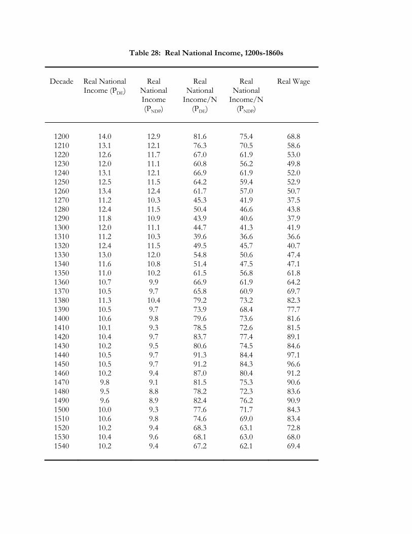
Table 28: Real National Income, 1200s-1860s
Decade
Real National Income (PDE)
Real
National Income (PNDP)
Real
National Income/N
(PDE)
Real
National Income/N
(PNDP)
Real Wage
1200 14.0 12.9 81.6 75.4 68.8 1210 13.1 12.1 76.3 70.5 58.6 1220 12.6 11.7 67.0 61.9 53.0 1230 12.0 11.1 60.8 56.2 49.8 1240 13.1 12.1 66.9 61.9 52.0 1250 12.5 11.5 64.2 59.4 52.9 1260 13.4 12.4 61.7 57.0 50.7 1270 11.2 10.3 45.3 41.9 37.5 1280 12.4 11.5 50.4 46.6 43.8 1290 11.8 10.9 43.9 40.6 37.9 1300 12.0 11.1 44.7 41.3 41.9 1310 11.2 10.3 39.6 36.6 36.6 1320 12.4 11.5 49.5 45.7 40.7 1330 13.0 12.0 54.8 50.6 47.4 1340 11.6 10.8 51.4 47.5 47.1 1350 11.0 10.2 61.5 56.8 61.8 1360 10.7 9.9 66.9 61.9 64.2 1370 10.5 9.7 65.8 60.9 69.7 1380 11.3 10.4 79.2 73.2 82.3 1390 10.5 9.7 73.9 68.4 77.7 1400 10.6 9.8 79.6 73.6 81.6 1410 10.1 9.3 78.5 72.6 81.5 1420 10.4 9.7 83.7 77.4 89.1 1430 10.2 9.5 80.6 74.5 84.6 1440 10.5 9.7 91.3 84.4 97.1 1450 10.5 9.7 91.2 84.3 96.6 1460 10.2 9.4 87.0 80.4 91.2 1470 9.8 9.1 81.5 75.3 90.6 1480 9.5 8.8 78.2 72.3 83.6 1490 9.6 8.9 82.4 76.2 90.9 1500 10.0 9.3 77.6 71.7 84.3 1510 10.6 9.8 74.6 69.0 83.4 1520 10.2 9.4 68.3 63.1 72.8 1530 10.4 9.6 68.1 63.0 68.0 1540 10.2 9.4 67.2 62.1 69.4
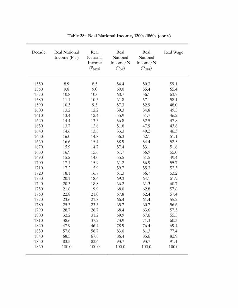
Table 28: Real National Income, 1200s-1860s (cont.)
Decade
Real National Income (PDE)
Real
National Income (PNDP)
Real
National Income/N
(PDE)
Real
National Income/N
(PNDP)
Real Wage
1550 8.9 8.3 54.4 50.3 59.1 1560 9.8 9.0 60.0 55.4 65.4 1570 10.8 10.0 60.7 56.1 63.7 1580 11.1 10.3 61.8 57.1 58.1 1590 10.3 9.5 57.3 52.9 48.0 1600 13.2 12.2 59.3 54.8 49.5 1610 13.4 12.4 55.9 51.7 46.2 1620 14.4 13.3 56.8 52.5 47.8 1630 13.7 12.6 51.8 47.9 43.8 1640 14.6 13.5 53.3 49.2 46.3 1650 16.0 14.8 56.3 52.1 51.1 1660 16.6 15.4 58.9 54.4 52.5 1670 15.9 14.7 57.4 53.1 51.6 1680 16.9 15.6 61.7 56.9 55.0 1690 15.2 14.0 55.5 51.5 49.4 1700 17.1 15.9 61.2 56.9 55.7 1710 17.2 15.9 59.7 55.3 52.3 1720 18.1 16.7 61.3 56.7 53.2 1730 20.1 18.6 69.3 64.1 61.9 1740 20.3 18.8 66.2 61.3 60.7 1750 21.6 19.9 68.0 62.8 57.6 1760 22.8 21.0 67.8 62.4 57.4 1770 23.6 21.8 66.4 61.4 55.2 1780 25.3 23.3 65.7 60.7 56.6 1790 28.7 26.7 68.4 63.6 57.5 1800 32.2 31.2 69.9 67.6 55.5 1810 38.6 37.2 73.9 71.3 60.3 1820 47.9 46.4 78.9 76.4 69.4 1830 57.8 56.7 83.0 81.3 77.4 1840 68.5 67.8 86.4 85.6 82.9 1850 83.5 83.6 93.7 93.7 91.1 1860 100.0 100.0 100.0 100.0 100.0
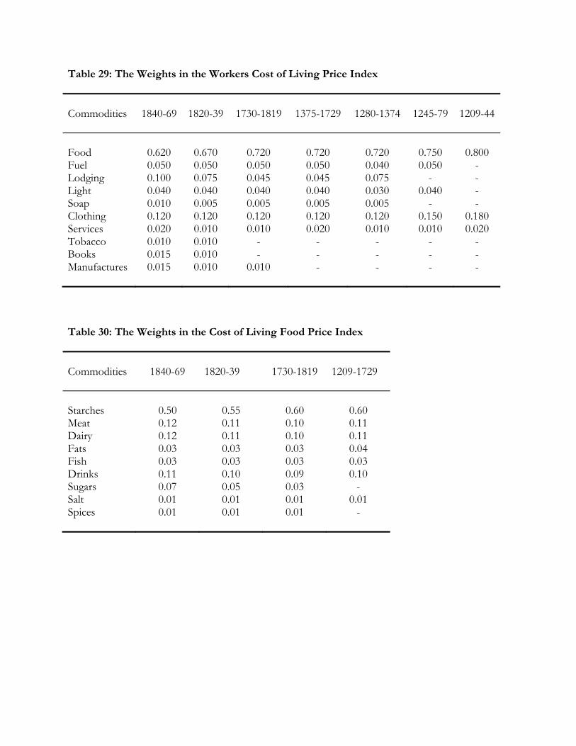
Table 29: The Weights in the Workers Cost of Living Price Index
Commodities
1840-69
1820-39
1730-1819
1375-1729
1280-1374
1245-79
1209-44
Food 0.620 0.670 0.720 0.720 0.720 0.750 0.800 Fuel 0.050 0.050 0.050 0.050 0.040 0.050 - Lodging 0.100 0.075 0.045 0.045 0.075 - - Light 0.040 0.040 0.040 0.040 0.030 0.040 - Soap 0.010 0.005 0.005 0.005 0.005 - - Clothing 0.120 0.120 0.120 0.120 0.120 0.150 0.180 Services 0.020 0.010 0.010 0.020 0.010 0.010 0.020 Tobacco 0.010 0.010 - - - - - Books 0.015 0.010 - - - - - Manufactures 0.015 0.010 0.010 - - - - Table 30: The Weights in the Cost of Living Food Price Index
Commodities
1840-69
1820-39
1730-1819
1209-1729
Starches 0.50 0.55 0.60 0.60 Meat 0.12 0.11 0.10 0.11 Dairy 0.12 0.11 0.10 0.11 Fats 0.03 0.03 0.03 0.04 Fish 0.03 0.03 0.03 0.03 Drinks 0.11 0.10 0.09 0.10 Sugars 0.07 0.05 0.03 - Salt 0.01 0.01 0.01 0.01 Spices 0.01 0.01 0.01 -
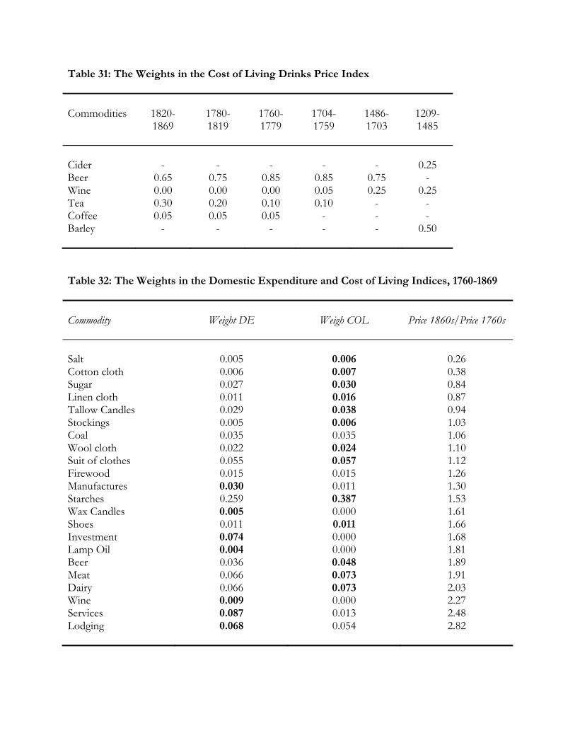
Table 31: The Weights in the Cost of Living Drinks Price Index
Commodities
1820-1869
1780-1819
1760-1779
1704-1759
1486-1703
1209-1485
Cider - - - - - 0.25 Beer 0.65 0.75 0.85 0.85 0.75 - Wine 0.00 0.00 0.00 0.05 0.25 0.25 Tea 0.30 0.20 0.10 0.10 - - Coffee 0.05 0.05 0.05 - - - Barley - - - - - 0.50 Table 32: The Weights in the Domestic Expenditure and Cost of Living Indices, 1760-1869
Commodity
Weight DE
Weigh COL
Price 1860s/Price 1760s
Salt 0.005 0.006 0.26 Cotton cloth 0.006 0.007 0.38 Sugar 0.027 0.030 0.84 Linen cloth 0.011 0.016 0.87 Tallow Candles 0.029 0.038 0.94 Stockings 0.005 0.006 1.03 Coal 0.035 0.035 1.06 Wool cloth 0.022 0.024 1.10 Suit of clothes 0.055 0.057 1.12 Firewood 0.015 0.015 1.26 Manufactures 0.030 0.011 1.30 Starches 0.259 0.387 1.53 Wax Candles 0.005 0.000 1.61 Shoes 0.011 0.011 1.66 Investment 0.074 0.000 1.68 Lamp Oil 0.004 0.000 1.81 Beer 0.036 0.048 1.89 Meat 0.066 0.073 1.91 Dairy 0.066 0.073 2.03 Wine 0.009 0.000 2.27 Services 0.087 0.013 2.48 Lodging 0.068 0.054 2.82
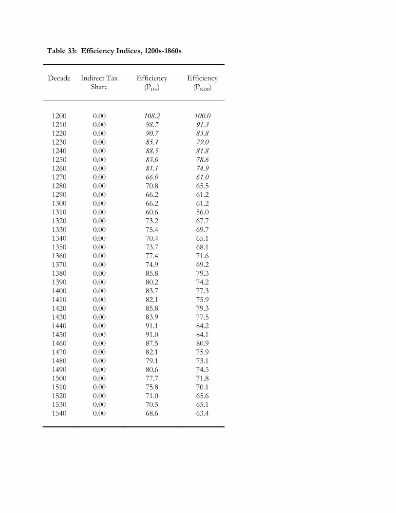
Table 33: Efficiency Indices, 1200s-1860s
Decade
Indirect Tax
Share
Efficiency
(PDE)
Efficiency
(PNDP)
1200 0.00 108.2 100.0 1210 0.00 98.7 91.3 1220 0.00 90.7 83.8 1230 0.00 85.4 79.0 1240 0.00 88.5 81.8 1250 0.00 85.0 78.6 1260 0.00 81.1 74.9 1270 0.00 66.0 61.0 1280 0.00 70.8 65.5 1290 0.00 66.2 61.2 1300 0.00 66.2 61.2 1310 0.00 60.6 56.0 1320 0.00 73.2 67.7 1330 0.00 75.4 69.7 1340 0.00 70.4 65.1 1350 0.00 73.7 68.1 1360 0.00 77.4 71.6 1370 0.00 74.9 69.2 1380 0.00 85.8 79.3 1390 0.00 80.2 74.2 1400 0.00 83.7 77.3 1410 0.00 82.1 75.9 1420 0.00 85.8 79.3 1430 0.00 83.9 77.5 1440 0.00 91.1 84.2 1450 0.00 91.0 84.1 1460 0.00 87.5 80.9 1470 0.00 82.1 75.9 1480 0.00 79.1 73.1 1490 0.00 80.6 74.5 1500 0.00 77.7 71.8 1510 0.00 75.8 70.1 1520 0.00 71.0 65.6 1530 0.00 70.5 65.1 1540 0.00 68.6 63.4
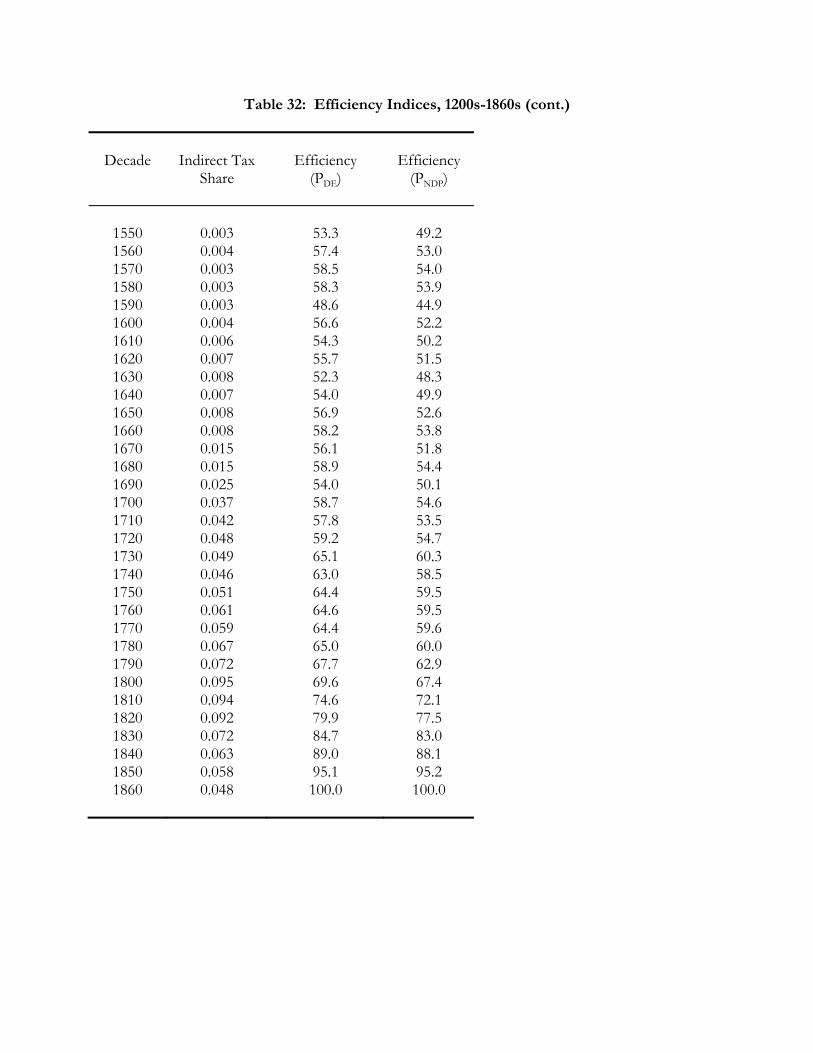
Table 32: Efficiency Indices, 1200s-1860s (cont.)
Decade
Indirect Tax
Share
Efficiency
(PDE)
Efficiency
(PNDP)
1550 0.003 53.3 49.2 1560 0.004 57.4 53.0 1570 0.003 58.5 54.0 1580 0.003 58.3 53.9 1590 0.003 48.6 44.9 1600 0.004 56.6 52.2 1610 0.006 54.3 50.2 1620 0.007 55.7 51.5 1630 0.008 52.3 48.3 1640 0.007 54.0 49.9 1650 0.008 56.9 52.6 1660 0.008 58.2 53.8 1670 0.015 56.1 51.8 1680 0.015 58.9 54.4 1690 0.025 54.0 50.1 1700 0.037 58.7 54.6 1710 0.042 57.8 53.5 1720 0.048 59.2 54.7 1730 0.049 65.1 60.3 1740 0.046 63.0 58.5 1750 0.051 64.4 59.5 1760 0.061 64.6 59.5 1770 0.059 64.4 59.6 1780 0.067 65.0 60.0 1790 0.072 67.7 62.9 1800 0.095 69.6 67.4 1810 0.094 74.6 72.1 1820 0.092 79.9 77.5 1830 0.072 84.7 83.0 1840 0.063 89.0 88.1 1850 0.058 95.1 95.2 1860 0.048 100.0 100.0
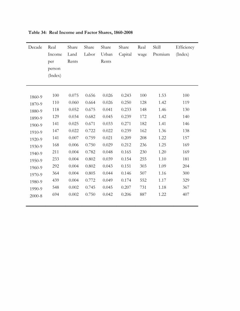
Table 34: Real Income and Factor Shares, 1860-2008
Decade Real
Income
per
person
(Index)
Share
Land
Rents
Share
Labor
Share
Urban
Rents
Share
Capital
Real
wage
Skill
Premium
Efficiency
(Index)
1860-9 100 0.075 0.656 0.026 0.243 100 1.53 100
1870-9 110 0.060 0.664 0.026 0.250 128 1.42 119
1880-9 118 0.052 0.675 0.041 0.233 148 1.46 130
1890-9 129 0.034 0.682 0.045 0.239 172 1.42 140
1900-9 141 0.025 0.671 0.033 0.271 182 1.41 146
1910-9 147 0.022 0.722 0.022 0.239 162 1.36 138
1920-9 141 0.007 0.759 0.021 0.209 208 1.22 157
1930-9 168 0.006 0.750 0.029 0.212 236 1.25 169
1940-9 211 0.004 0.782 0.048 0.165 230 1.20 169
1950-9 233 0.004 0.802 0.039 0.154 255 1.10 181
1960-9 292 0.004 0.802 0.043 0.151 303 1.09 204
1970-9 364 0.004 0.805 0.044 0.146 507 1.16 300
1980-9 439 0.004 0.772 0.049 0.174 552 1.17 329
1990-9 548 0.002 0.745 0.045 0.207 731 1.18 367
2000-8 694 0.002 0.750 0.042 0.206 887 1.22 407
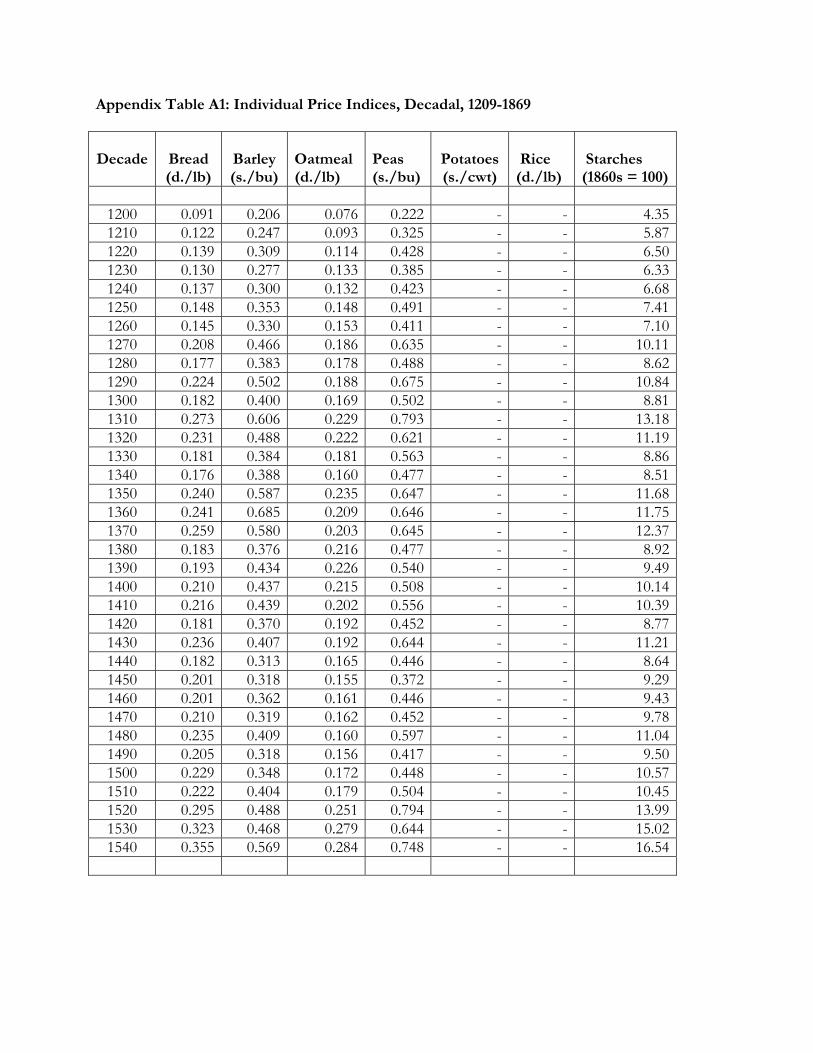
Appendix Table A1: Individual Price Indices, Decadal, 1209-1869
Decade
Bread (d./lb)
Barley (s./bu)
Oatmeal (d./lb)
Peas (s./bu)
Potatoes (s./cwt)
Rice (d./lb)
Starches (1860s = 100)
1200 0.091 0.206 0.076 0.222 - - 4.351210 0.122 0.247 0.093 0.325 - - 5.871220 0.139 0.309 0.114 0.428 - - 6.501230 0.130 0.277 0.133 0.385 - - 6.331240 0.137 0.300 0.132 0.423 - - 6.681250 0.148 0.353 0.148 0.491 - - 7.411260 0.145 0.330 0.153 0.411 - - 7.101270 0.208 0.466 0.186 0.635 - - 10.111280 0.177 0.383 0.178 0.488 - - 8.621290 0.224 0.502 0.188 0.675 - - 10.841300 0.182 0.400 0.169 0.502 - - 8.811310 0.273 0.606 0.229 0.793 - - 13.181320 0.231 0.488 0.222 0.621 - - 11.191330 0.181 0.384 0.181 0.563 - - 8.861340 0.176 0.388 0.160 0.477 - - 8.511350 0.240 0.587 0.235 0.647 - - 11.681360 0.241 0.685 0.209 0.646 - - 11.751370 0.259 0.580 0.203 0.645 - - 12.371380 0.183 0.376 0.216 0.477 - - 8.921390 0.193 0.434 0.226 0.540 - - 9.491400 0.210 0.437 0.215 0.508 - - 10.141410 0.216 0.439 0.202 0.556 - - 10.391420 0.181 0.370 0.192 0.452 - - 8.771430 0.236 0.407 0.192 0.644 - - 11.211440 0.182 0.313 0.165 0.446 - - 8.641450 0.201 0.318 0.155 0.372 - - 9.291460 0.201 0.362 0.161 0.446 - - 9.431470 0.210 0.319 0.162 0.452 - - 9.781480 0.235 0.409 0.160 0.597 - - 11.041490 0.205 0.318 0.156 0.417 - - 9.501500 0.229 0.348 0.172 0.448 - - 10.571510 0.222 0.404 0.179 0.504 - - 10.451520 0.295 0.488 0.251 0.794 - - 13.991530 0.323 0.468 0.279 0.644 - - 15.021540 0.355 0.569 0.284 0.748 - - 16.54
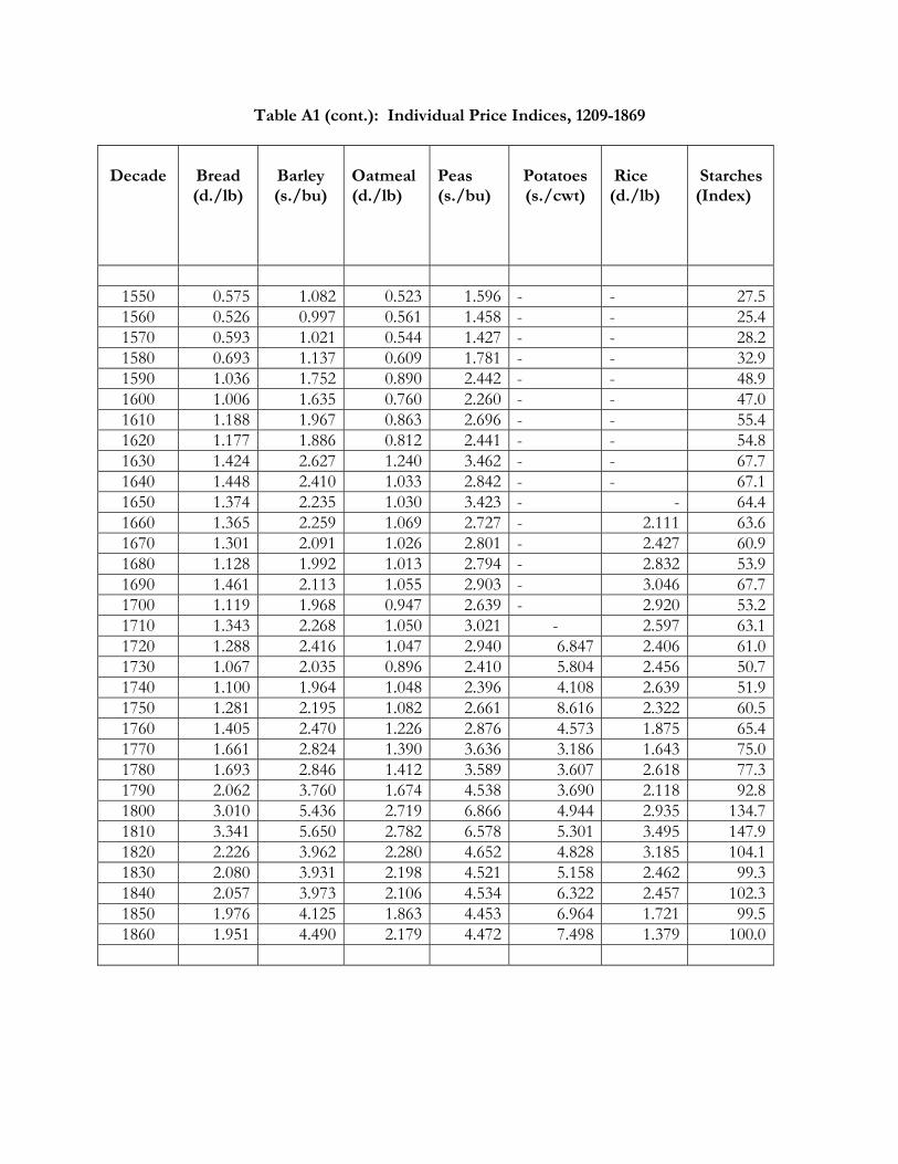
Table A1 (cont.): Individual Price Indices, 1209-1869
Decade
Bread (d./lb)
Barley (s./bu)
Oatmeal (d./lb)
Peas (s./bu)
Potatoes (s./cwt)
Rice (d./lb)
Starches (Index)
1550 0.575 1.082 0.523 1.596 - - 27.51560 0.526 0.997 0.561 1.458 - - 25.41570 0.593 1.021 0.544 1.427 - - 28.21580 0.693 1.137 0.609 1.781 - - 32.91590 1.036 1.752 0.890 2.442 - - 48.91600 1.006 1.635 0.760 2.260 - - 47.01610 1.188 1.967 0.863 2.696 - - 55.41620 1.177 1.886 0.812 2.441 - - 54.81630 1.424 2.627 1.240 3.462 - - 67.71640 1.448 2.410 1.033 2.842 - - 67.11650 1.374 2.235 1.030 3.423 - - 64.41660 1.365 2.259 1.069 2.727 - 2.111 63.61670 1.301 2.091 1.026 2.801 - 2.427 60.91680 1.128 1.992 1.013 2.794 - 2.832 53.91690 1.461 2.113 1.055 2.903 - 3.046 67.71700 1.119 1.968 0.947 2.639 - 2.920 53.21710 1.343 2.268 1.050 3.021 - 2.597 63.11720 1.288 2.416 1.047 2.940 6.847 2.406 61.01730 1.067 2.035 0.896 2.410 5.804 2.456 50.71740 1.100 1.964 1.048 2.396 4.108 2.639 51.91750 1.281 2.195 1.082 2.661 8.616 2.322 60.51760 1.405 2.470 1.226 2.876 4.573 1.875 65.41770 1.661 2.824 1.390 3.636 3.186 1.643 75.01780 1.693 2.846 1.412 3.589 3.607 2.618 77.31790 2.062 3.760 1.674 4.538 3.690 2.118 92.81800 3.010 5.436 2.719 6.866 4.944 2.935 134.71810 3.341 5.650 2.782 6.578 5.301 3.495 147.91820 2.226 3.962 2.280 4.652 4.828 3.185 104.11830 2.080 3.931 2.198 4.521 5.158 2.462 99.31840 2.057 3.973 2.106 4.534 6.322 2.457 102.31850 1.976 4.125 1.863 4.453 6.964 1.721 99.51860 1.951 4.490 2.179 4.472 7.498 1.379 100.0
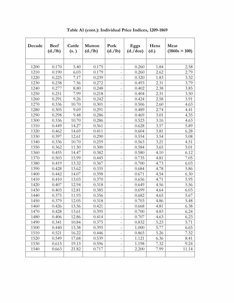
Table A1 (cont.): Individual Price Indices, 1209-1869
Decade
Beef
(d./lb)
Cattle (s. )
Mutton (d./lb)
Pork (d./lb)
Eggs
(d./doz)
Hens (d.)
Meat (1860s = 100)
1200 0.170 5.40 0.175 - 0.260 1.84 2.581210 0.190 6.03 0.179 - 0.260 2.62 2.791220 0.225 7.17 0.239 - 0.320 1.83 3.321230 0.238 7.56 0.272 - 0.493 2.31 3.791240 0.277 8.80 0.248 - 0.402 2.38 3.851250 0.251 7.99 0.218 - 0.404 2.31 3.501260 0.291 9.26 0.242 - 0.424 2.58 3.911270 0.336 10.70 0.301 - 0.506 2.60 4.631280 0.305 9.69 0.291 - 0.489 2.74 4.411290 0.298 9.48 0.286 - 0.469 3.01 4.351300 0.336 10.70 0.286 - 0.523 3.16 4.631310 0.449 14.27 0.361 - 0.628 3.57 5.891320 0.462 14.69 0.411 - 0.604 3.81 6.281330 0.397 12.61 0.290 - 0.554 3.54 5.081340 0.336 10.70 0.259 - 0.563 3.21 4.511350 0.362 11.50 0.300 - 0.584 3.65 5.011360 0.455 14.47 0.382 - 0.580 4.10 6.121370 0.503 15.99 0.445 - 0.735 4.81 7.051380 0.419 13.32 0.367 - 0.700 4.73 6.031390 0.428 13.62 0.335 - 0.684 4.78 5.861400 0.442 14.07 0.398 - 0.671 4.54 6.301410 0.410 13.03 0.370 - 0.656 4.71 5.951420 0.407 12.94 0.318 - 0.649 4.56 5.561430 0.403 12.81 0.385 - 0.699 4.64 6.031440 0.375 11.93 0.356 - 0.682 4.65 5.671450 0.379 12.05 0.318 - 0.703 4.86 5.481460 0.426 13.56 0.421 - 0.668 4.81 6.381470 0.428 13.61 0.395 - 0.700 4.83 6.241480 0.406 12.86 0.414 - 0.707 4.63 6.231490 0.341 10.84 0.375 - 0.832 5.23 5.711500 0.440 13.38 0.395 - 1.000 5.77 6.651510 0.521 16.22 0.446 - 0.865 5.26 7.321520 0.549 17.68 0.539 - 1.121 6.36 8.411530 0.615 19.13 0.596 - 1.198 7.32 9.241540 0.663 21.82 0.717 - 2.200 7.99 11.14
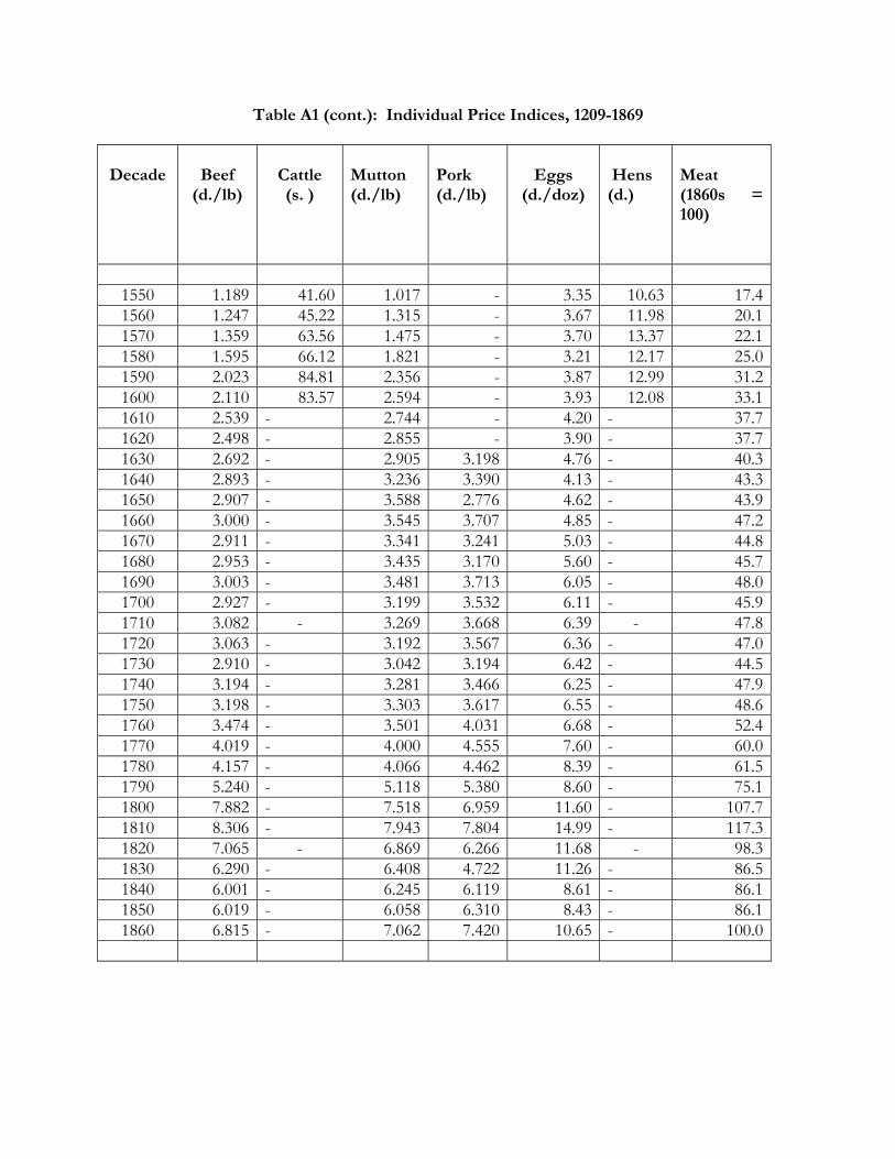
Table A1 (cont.): Individual Price Indices, 1209-1869
Decade
Beef
(d./lb)
Cattle (s. )
Mutton (d./lb)
Pork (d./lb)
Eggs
(d./doz)
Hens (d.)
Meat (1860s = 100)
1550 1.189 41.60 1.017 - 3.35 10.63 17.41560 1.247 45.22 1.315 - 3.67 11.98 20.11570 1.359 63.56 1.475 - 3.70 13.37 22.11580 1.595 66.12 1.821 - 3.21 12.17 25.01590 2.023 84.81 2.356 - 3.87 12.99 31.21600 2.110 83.57 2.594 - 3.93 12.08 33.11610 2.539 - 2.744 - 4.20 - 37.71620 2.498 - 2.855 - 3.90 - 37.71630 2.692 - 2.905 3.198 4.76 - 40.31640 2.893 - 3.236 3.390 4.13 - 43.31650 2.907 - 3.588 2.776 4.62 - 43.91660 3.000 - 3.545 3.707 4.85 - 47.21670 2.911 - 3.341 3.241 5.03 - 44.81680 2.953 - 3.435 3.170 5.60 - 45.71690 3.003 - 3.481 3.713 6.05 - 48.01700 2.927 - 3.199 3.532 6.11 - 45.91710 3.082 - 3.269 3.668 6.39 - 47.81720 3.063 - 3.192 3.567 6.36 - 47.01730 2.910 - 3.042 3.194 6.42 - 44.51740 3.194 - 3.281 3.466 6.25 - 47.91750 3.198 - 3.303 3.617 6.55 - 48.61760 3.474 - 3.501 4.031 6.68 - 52.41770 4.019 - 4.000 4.555 7.60 - 60.01780 4.157 - 4.066 4.462 8.39 - 61.51790 5.240 - 5.118 5.380 8.60 - 75.11800 7.882 - 7.518 6.959 11.60 - 107.71810 8.306 - 7.943 7.804 14.99 - 117.31820 7.065 - 6.869 6.266 11.68 - 98.31830 6.290 - 6.408 4.722 11.26 - 86.51840 6.001 - 6.245 6.119 8.61 - 86.11850 6.019 - 6.058 6.310 8.43 - 86.11860 6.815 - 7.062 7.420 10.65 - 100.0
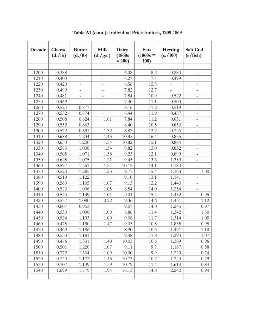
Table A1 (cont.): Individual Price Indices, 1209-1869
Decade
Cheese (d./lb)
Butter (d./lb)
Milk
(d./ga )
Dairy (1860s = 100)
Fats
(1860s = 100)
Herring (s./100)
Salt Cod (s/fish)
1200 0.388 - - 6.08 8.2 0.280 - 1210 0.400 - - 6.27 7.4 0.499 - 1220 0.420 - - 6.56 15.5 - - 1230 0.499 - - 7.82 12.7 - - 1240 0.481 - - 7.54 10.9 0.522 - 1250 0.469 - - 7.40 11.1 0.503 - 1260 0.524 0.877 - 8.16 11.2 0.519 - 1270 0.552 0.874 - 8.44 11.9 0.457 - 1280 0.508 0.824 1.01 7.84 11.2 0.651 - 1290 0.552 0.863 8.40 10.5 0.650 - 1300 0.572 0.891 1.32 8.82 12.7 0.726 - 1310 0.688 1.234 1.43 10.85 16.4 0.855 - 1320 0.650 1.200 1.54 10.82 15.1 0.884 - 1330 0.583 1.008 1.54 9.82 13.0 0.832 - 1340 0.505 1.071 1.38 9.23 12.1 0.899 - 1350 0.625 1.075 1.21 9.45 13.6 1.339 - 1360 0.597 1.261 1.24 10.12 14.1 1.180 - 1370 0.520 1.285 1.23 9.77 15.4 1.163 1.001380 0.519 1.122 9.10 13.1 1.141 - 1390 0.560 1.105 1.07 9.13 12.2 1.440 - 1400 0.523 1.006 1.05 8.54 14.0 1.254 - 1410 0.546 1.149 1.01 9.01 15.4 1.432 0.951420 0.537 1.080 2.22 9.36 14.6 1.431 1.121430 0.607 0.953 9.07 14.0 1.245 0.971440 0.530 1.098 1.00 8.86 11.4 1.342 1.301450 0.524 1.193 1.00 9.08 11.7 1.314 1.051460 0.475 1.190 1.47 9.05 10.8 1.835 0.951470 0.469 1.186 8.90 10.3 1.491 1.101480 0.533 1.181 9.48 11.8 1.294 1.071490 0.476 1.331 1.48 10.03 10.6 1.389 0.961500 0.501 1.220 1.07 9.11 9.7 1.187 0.581510 0.772 1.304 1.09 10.00 9.9 1.229 0.741520 0.740 1.172 1.43 10.73 10.2 1.244 0.791530 0.707 1.139 1.59 10.79 11.4 1.614 0.841540 1.699 1.779 1.94 16.13 14.8 2.242 0.94
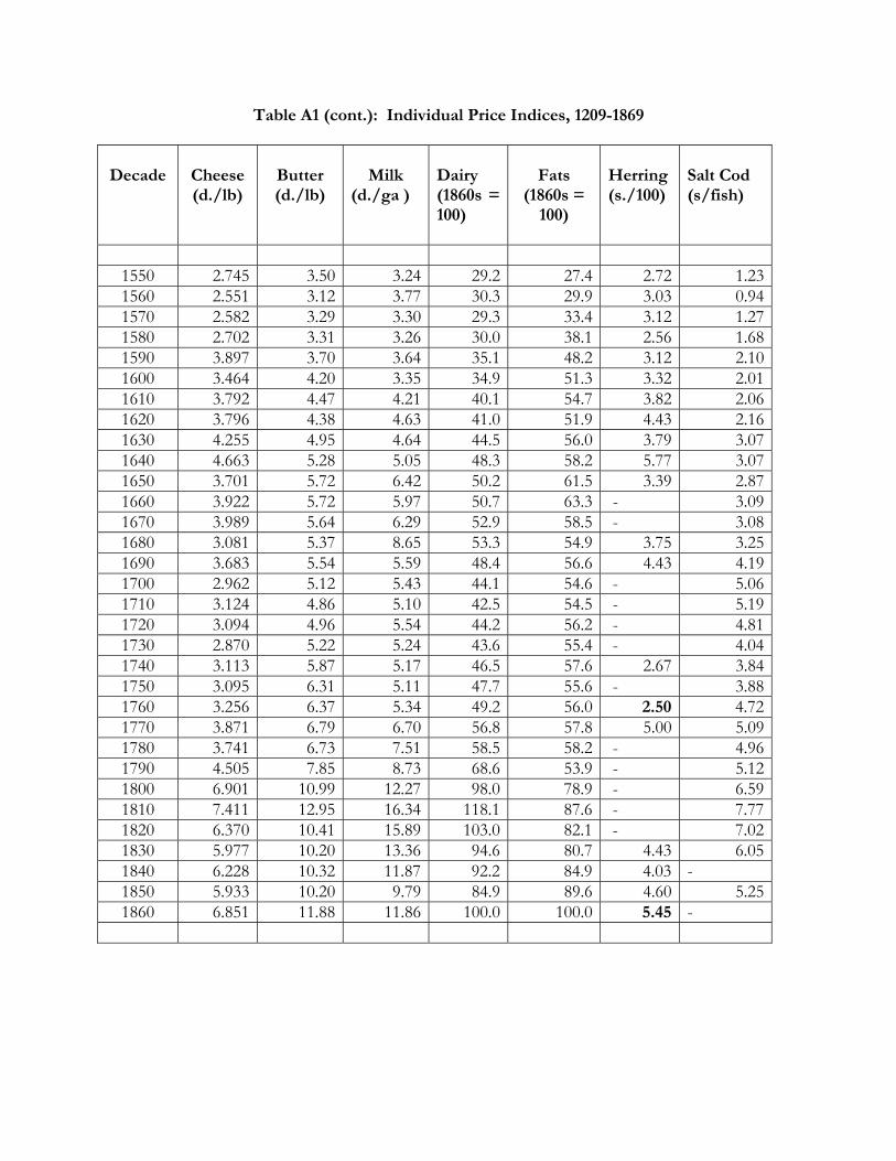
Table A1 (cont.): Individual Price Indices, 1209-1869
Decade
Cheese (d./lb)
Butter (d./lb)
Milk
(d./ga )
Dairy (1860s = 100)
Fats
(1860s = 100)
Herring (s./100)
Salt Cod (s/fish)
1550 2.745 3.50 3.24 29.2 27.4 2.72 1.231560 2.551 3.12 3.77 30.3 29.9 3.03 0.941570 2.582 3.29 3.30 29.3 33.4 3.12 1.271580 2.702 3.31 3.26 30.0 38.1 2.56 1.681590 3.897 3.70 3.64 35.1 48.2 3.12 2.101600 3.464 4.20 3.35 34.9 51.3 3.32 2.011610 3.792 4.47 4.21 40.1 54.7 3.82 2.061620 3.796 4.38 4.63 41.0 51.9 4.43 2.161630 4.255 4.95 4.64 44.5 56.0 3.79 3.071640 4.663 5.28 5.05 48.3 58.2 5.77 3.071650 3.701 5.72 6.42 50.2 61.5 3.39 2.871660 3.922 5.72 5.97 50.7 63.3 - 3.091670 3.989 5.64 6.29 52.9 58.5 - 3.081680 3.081 5.37 8.65 53.3 54.9 3.75 3.251690 3.683 5.54 5.59 48.4 56.6 4.43 4.191700 2.962 5.12 5.43 44.1 54.6 - 5.061710 3.124 4.86 5.10 42.5 54.5 - 5.191720 3.094 4.96 5.54 44.2 56.2 - 4.811730 2.870 5.22 5.24 43.6 55.4 - 4.041740 3.113 5.87 5.17 46.5 57.6 2.67 3.841750 3.095 6.31 5.11 47.7 55.6 - 3.881760 3.256 6.37 5.34 49.2 56.0 2.50 4.721770 3.871 6.79 6.70 56.8 57.8 5.00 5.091780 3.741 6.73 7.51 58.5 58.2 - 4.961790 4.505 7.85 8.73 68.6 53.9 - 5.121800 6.901 10.99 12.27 98.0 78.9 - 6.591810 7.411 12.95 16.34 118.1 87.6 - 7.771820 6.370 10.41 15.89 103.0 82.1 - 7.021830 5.977 10.20 13.36 94.6 80.7 4.43 6.051840 6.228 10.32 11.87 92.2 84.9 4.03 - 1850 5.933 10.20 9.79 84.9 89.6 4.60 5.251860 6.851 11.88 11.86 100.0 100.0 5.45 -
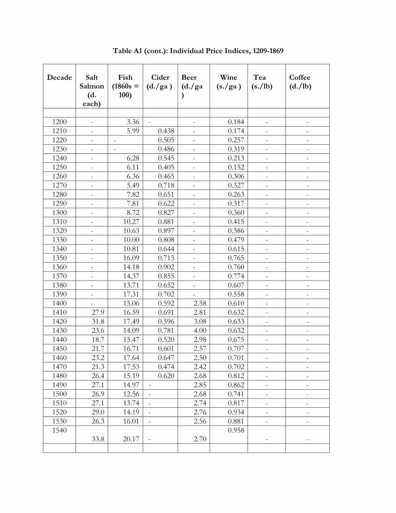
Table A1 (cont.): Individual Price Indices, 1209-1869
Decade
Salt
Salmon (d.
each)
Fish
(1860s = 100)
Cider
(d./ga )
Beer (d./ga )
Wine
(s./ga )
Tea (s./lb)
Coffee (d./lb)
1200 - 3.36 - - 0.184 - - 1210 - 5.99 0.438 - 0.174 - - 1220 - - 0.505 - 0.257 - - 1230 - - 0.486 - 0.319 - - 1240 - 6.28 0.545 - 0.213 - - 1250 - 6.11 0.405 - 0.152 - - 1260 - 6.36 0.465 - 0.306 - - 1270 - 5.49 0.718 - 0.327 - - 1280 - 7.82 0.651 - 0.263 - - 1290 - 7.81 0.622 - 0.317 - - 1300 - 8.72 0.827 - 0.360 - - 1310 - 10.27 0.881 - 0.415 - - 1320 - 10.63 0.897 - 0.386 - - 1330 - 10.00 0.808 - 0.479 - - 1340 - 10.81 0.644 - 0.615 - - 1350 - 16.09 0.713 - 0.765 - - 1360 - 14.18 0.902 - 0.760 - - 1370 - 14.37 0.855 - 0.774 - - 1380 - 13.71 0.652 - 0.607 - - 1390 - 17.31 0.702 - 0.558 - - 1400 - 15.06 0.592 2.58 0.610 - - 1410 27.9 16.59 0.691 2.81 0.632 - - 1420 31.8 17.49 0.596 3.08 0.633 - - 1430 23.6 14.09 0.781 4.00 0.632 - - 1440 18.7 15.47 0.520 2.98 0.675 - - 1450 21.7 16.71 0.601 2.57 0.707 - - 1460 23.2 17.64 0.647 2.50 0.701 - - 1470 21.3 17.53 0.474 2.42 0.702 - - 1480 26.4 15.19 0.620 2.68 0.812 - - 1490 27.1 14.97 - 2.85 0.862 - - 1500 26.9 12.56 - 2.68 0.741 - - 1510 27.1 13.74 - 2.74 0.817 - - 1520 29.0 14.19 - 2.76 0.934 - - 1530 26.3 16.01 - 2.56 0.881 - - 1540
33.8 20.17 - 2.700.958
- -
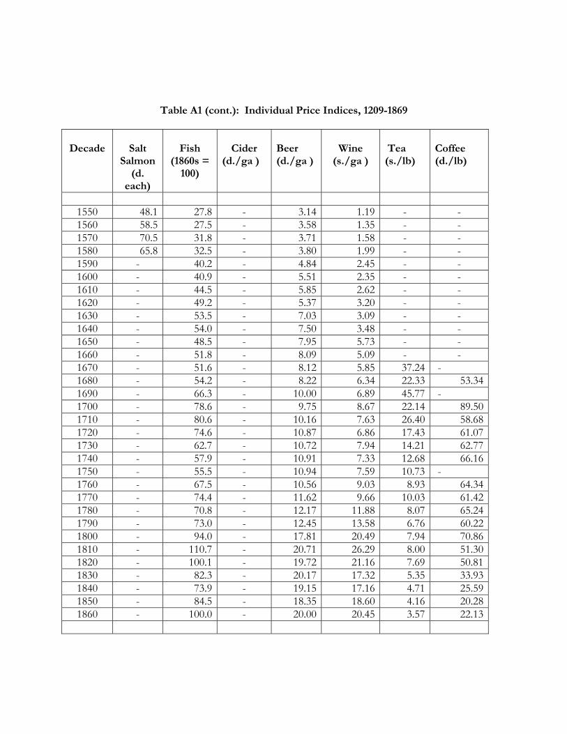
Table A1 (cont.): Individual Price Indices, 1209-1869
Decade
Salt
Salmon (d.
each)
Fish
(1860s = 100)
Cider
(d./ga )
Beer (d./ga )
Wine
(s./ga )
Tea (s./lb)
Coffee (d./lb)
1550 48.1 27.8 - 3.14 1.19 - - 1560 58.5 27.5 - 3.58 1.35 - - 1570 70.5 31.8 - 3.71 1.58 - - 1580 65.8 32.5 - 3.80 1.99 - - 1590 - 40.2 - 4.84 2.45 - - 1600 - 40.9 - 5.51 2.35 - - 1610 - 44.5 - 5.85 2.62 - - 1620 - 49.2 - 5.37 3.20 - - 1630 - 53.5 - 7.03 3.09 - - 1640 - 54.0 - 7.50 3.48 - - 1650 - 48.5 - 7.95 5.73 - - 1660 - 51.8 - 8.09 5.09 - - 1670 - 51.6 - 8.12 5.85 37.24 - 1680 - 54.2 - 8.22 6.34 22.33 53.341690 - 66.3 - 10.00 6.89 45.77 - 1700 - 78.6 - 9.75 8.67 22.14 89.501710 - 80.6 - 10.16 7.63 26.40 58.681720 - 74.6 - 10.87 6.86 17.43 61.071730 - 62.7 - 10.72 7.94 14.21 62.771740 - 57.9 - 10.91 7.33 12.68 66.161750 - 55.5 - 10.94 7.59 10.73 - 1760 - 67.5 - 10.56 9.03 8.93 64.341770 - 74.4 - 11.62 9.66 10.03 61.421780 - 70.8 - 12.17 11.88 8.07 65.241790 - 73.0 - 12.45 13.58 6.76 60.221800 - 94.0 - 17.81 20.49 7.94 70.861810 - 110.7 - 20.71 26.29 8.00 51.301820 - 100.1 - 19.72 21.16 7.69 50.811830 - 82.3 - 20.17 17.32 5.35 33.931840 - 73.9 - 19.15 17.16 4.71 25.591850 - 84.5 - 18.35 18.60 4.16 20.281860 - 100.0 - 20.00 20.45 3.57 22.13
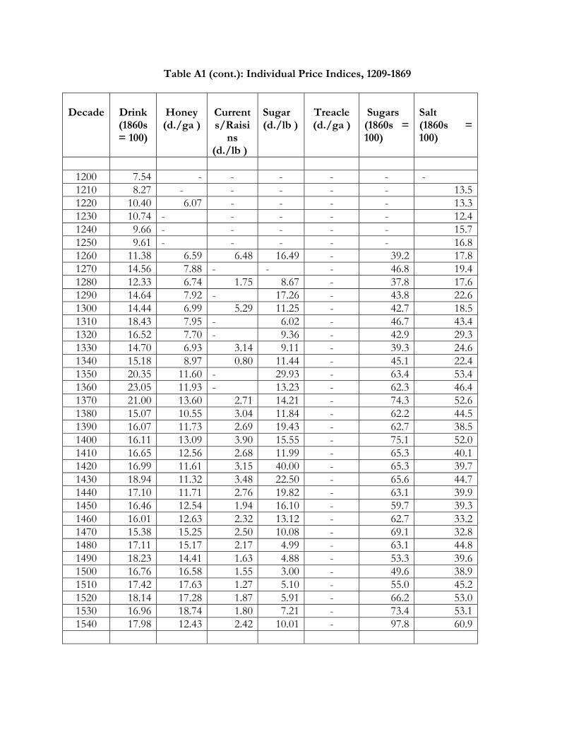
Table A1 (cont.): Individual Price Indices, 1209-1869
Decade
Drink (1860s = 100)
Honey (d./ga )
Currents/Raisi
ns (d./lb )
Sugar (d./lb )
Treacle (d./ga )
Sugars (1860s = 100)
Salt (1860s = 100)
1200 7.54 - - - - - - 1210 8.27 - - - - - 13.51220 10.40 6.07 - - - - 13.31230 10.74 - - - - - 12.41240 9.66 - - - - - 15.71250 9.61 - - - - - 16.81260 11.38 6.59 6.48 16.49 - 39.2 17.81270 14.56 7.88 - - - 46.8 19.41280 12.33 6.74 1.75 8.67 - 37.8 17.61290 14.64 7.92 - 17.26 - 43.8 22.61300 14.44 6.99 5.29 11.25 - 42.7 18.51310 18.43 7.95 - 6.02 - 46.7 43.41320 16.52 7.70 - 9.36 - 42.9 29.31330 14.70 6.93 3.14 9.11 - 39.3 24.61340 15.18 8.97 0.80 11.44 - 45.1 22.41350 20.35 11.60 - 29.93 - 63.4 53.41360 23.05 11.93 - 13.23 - 62.3 46.41370 21.00 13.60 2.71 14.21 - 74.3 52.61380 15.07 10.55 3.04 11.84 - 62.2 44.51390 16.07 11.73 2.69 19.43 - 62.7 38.51400 16.11 13.09 3.90 15.55 - 75.1 52.01410 16.65 12.56 2.68 11.99 - 65.3 40.11420 16.99 11.61 3.15 40.00 - 65.3 39.71430 18.94 11.32 3.48 22.50 - 65.6 44.71440 17.10 11.71 2.76 19.82 - 63.1 39.91450 16.46 12.54 1.94 16.10 - 59.7 39.31460 16.01 12.63 2.32 13.12 - 62.7 33.21470 15.38 15.25 2.50 10.08 - 69.1 32.81480 17.11 15.17 2.17 4.99 - 63.1 44.81490 18.23 14.41 1.63 4.88 - 53.3 39.61500 16.76 16.58 1.55 3.00 - 49.6 38.91510 17.42 17.63 1.27 5.10 - 55.0 45.21520 18.14 17.28 1.87 5.91 - 66.2 53.01530 16.96 18.74 1.80 7.21 - 73.4 53.11540 17.98 12.43 2.42 10.01 - 97.8 60.9
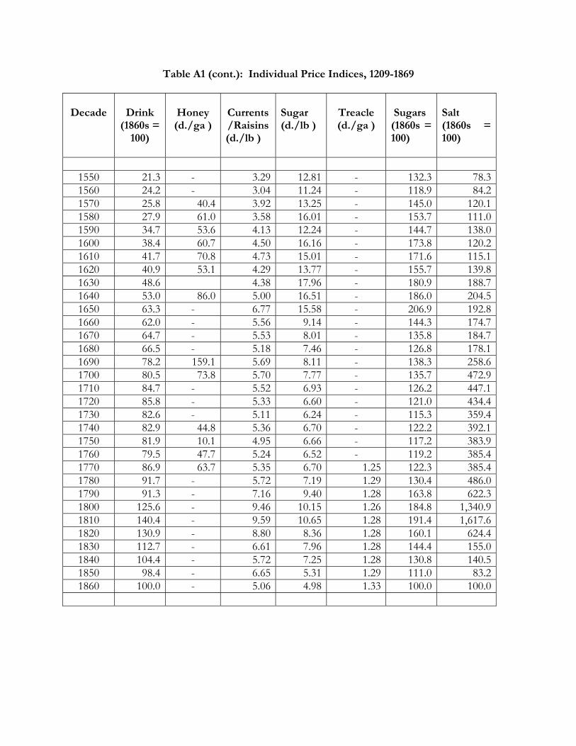
Table A1 (cont.): Individual Price Indices, 1209-1869
Decade
Drink
(1860s = 100)
Honey (d./ga )
Currents/Raisins (d./lb )
Sugar (d./lb )
Treacle (d./ga )
Sugars (1860s = 100)
Salt (1860s = 100)
1550 21.3 - 3.29 12.81 - 132.3 78.31560 24.2 - 3.04 11.24 - 118.9 84.21570 25.8 40.4 3.92 13.25 - 145.0 120.11580 27.9 61.0 3.58 16.01 - 153.7 111.01590 34.7 53.6 4.13 12.24 - 144.7 138.01600 38.4 60.7 4.50 16.16 - 173.8 120.21610 41.7 70.8 4.73 15.01 - 171.6 115.11620 40.9 53.1 4.29 13.77 - 155.7 139.81630 48.6 4.38 17.96 - 180.9 188.71640 53.0 86.0 5.00 16.51 - 186.0 204.51650 63.3 - 6.77 15.58 - 206.9 192.81660 62.0 - 5.56 9.14 - 144.3 174.71670 64.7 - 5.53 8.01 - 135.8 184.71680 66.5 - 5.18 7.46 - 126.8 178.11690 78.2 159.1 5.69 8.11 - 138.3 258.61700 80.5 73.8 5.70 7.77 - 135.7 472.91710 84.7 - 5.52 6.93 - 126.2 447.11720 85.8 - 5.33 6.60 - 121.0 434.41730 82.6 - 5.11 6.24 - 115.3 359.41740 82.9 44.8 5.36 6.70 - 122.2 392.11750 81.9 10.1 4.95 6.66 - 117.2 383.91760 79.5 47.7 5.24 6.52 - 119.2 385.41770 86.9 63.7 5.35 6.70 1.25 122.3 385.41780 91.7 - 5.72 7.19 1.29 130.4 486.01790 91.3 - 7.16 9.40 1.28 163.8 622.31800 125.6 - 9.46 10.15 1.26 184.8 1,340.91810 140.4 - 9.59 10.65 1.28 191.4 1,617.61820 130.9 - 8.80 8.36 1.28 160.1 624.41830 112.7 - 6.61 7.96 1.28 144.4 155.01840 104.4 - 5.72 7.25 1.28 130.8 140.51850 98.4 - 6.65 5.31 1.29 111.0 83.21860 100.0 - 5.06 4.98 1.33 100.0 100.0
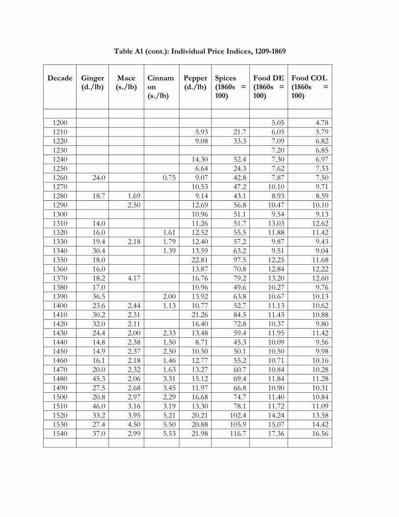
Table A1 (cont.): Individual Price Indices, 1209-1869
Decade
Ginger (d./lb)
Mace (s./lb)
Cinnamon (s./lb)
Pepper (d./lb)
Spices (1860s = 100)
Food DE (1860s = 100)
Food COL (1860s = 100)
1200 5.05 4.781210 5.93 21.7 6.05 5.791220 9.08 33.3 7.09 6.821230 7.20 6.851240 14.30 52.4 7.30 6.971250 6.64 24.3 7.62 7.331260 24.0 0.75 9.07 42.8 7.87 7.501270 10.53 47.2 10.10 9.711280 18.7 1.69 9.14 43.1 8.93 8.591290 2.50 12.69 56.8 10.47 10.101300 10.96 51.1 9.54 9.131310 14.0 11.26 51.7 13.03 12.621320 16.0 1.61 12.52 55.5 11.88 11.421330 19.4 2.18 1.79 12.40 57.2 9.87 9.431340 30.4 1.39 13.59 63.2 9.51 9.041350 18.0 22.81 97.5 12.25 11.681360 16.0 13.87 70.8 12.84 12.221370 18.2 4.17 16.76 79.2 13.20 12.601380 17.0 10.96 49.6 10.27 9.761390 36.5 2.00 13.92 63.8 10.67 10.131400 23.6 2.44 1.13 10.77 52.7 11.13 10.621410 30.2 2.31 21.26 84.5 11.43 10.881420 32.0 2.11 16.40 72.8 10.37 9.801430 24.4 2.00 2.33 13.48 59.4 11.95 11.421440 14.8 2.38 1.50 8.71 45.3 10.09 9.561450 14.9 2.37 2.50 10.50 50.1 10.50 9.981460 16.1 2.18 1.46 12.77 55.2 10.71 10.161470 20.0 2.32 1.63 13.27 60.7 10.84 10.281480 45.3 2.06 3.31 15.12 69.4 11.84 11.281490 27.5 2.68 3.45 11.97 66.8 10.90 10.311500 20.8 2.97 2.29 16.68 74.7 11.40 10.841510 46.0 3.16 3.19 13.30 78.1 11.72 11.091520 33.2 3.95 5.21 20.21 102.4 14.24 13.581530 27.4 4.50 5.50 20.88 105.9 15.07 14.421540 37.0 2.99 5.53 21.98 116.7 17.36 16.56
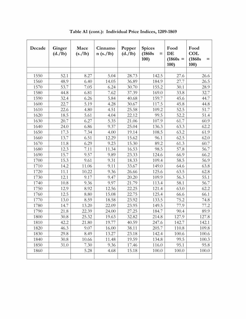
Table A1 (cont.): Individual Price Indices, 1209-1869
Decade
Ginger (d./lb)
Mace (s./lb)
Cinnamon (s./lb)
Pepper (d./lb)
Spices (1860s = 100)
Food DE (1860s = 100)
Food COL (1860s = 100)
1550 52.1 8.27 5.04 28.73 142.5 27.6 26.61560 48.9 6.40 14.05 36.89 184.9 27.7 26.51570 53.7 7.05 6.24 30.70 155.2 30.1 28.91580 44.8 6.81 7.62 37.39 169.0 33.8 32.71590 32.4 6.26 5.84 40.68 159.7 45.6 44.71600 22.7 5.19 4.28 30.67 117.5 45.8 44.81610 22.6 4.80 4.51 25.58 109.2 52.5 51.71620 18.5 5.61 4.04 22.12 99.5 52.2 51.41630 20.7 6.27 5.35 21.06 107.9 61.7 60.91640 24.0 6.86 9.37 25.04 136.3 63.3 62.21650 17.3 7.34 4.00 19.14 108.5 63.2 61.91660 13.7 6.51 12.29 15.62 96.1 62.5 62.01670 11.8 6.29 9.23 15.30 89.2 61.3 60.71680 12.3 7.11 11.34 16.53 98.5 57.8 56.71690 15.7 9.57 9.89 23.33 124.6 66.9 66.21700 15.3 9.61 9.31 18.33 109.4 58.5 56.91710 14.2 11.06 9.11 33.67 149.0 64.6 63.81720 11.1 10.22 9.36 26.66 125.6 63.5 62.81730 12.1 9.17 9.47 20.20 109.9 56.3 55.11740 10.8 9.36 9.97 21.79 113.4 58.1 56.71750 12.9 8.92 12.56 22.25 121.4 63.0 62.21760 12.5 8.80 15.08 22.75 125.4 66.6 66.11770 13.0 8.59 18.58 23.92 133.5 75.2 74.81780 14.7 13.20 22.09 23.95 149.5 77.9 77.21790 21.8 22.39 24.00 27.25 184.7 90.4 89.91800 30.8 25.32 19.63 32.82 214.8 127.9 127.81810 42.2 21.80 19.77 40.59 247.6 142.7 142.11820 46.3 9.07 16.00 38.11 205.7 110.8 109.81830 29.8 8.49 13.27 23.18 142.4 100.6 100.61840 30.8 10.66 11.48 19.59 134.8 99.5 100.31850 31.0 7.30 9.36 17.46 116.0 95.1 95.81860 5.28 4.68 15.18 100.0 100.0 100.0
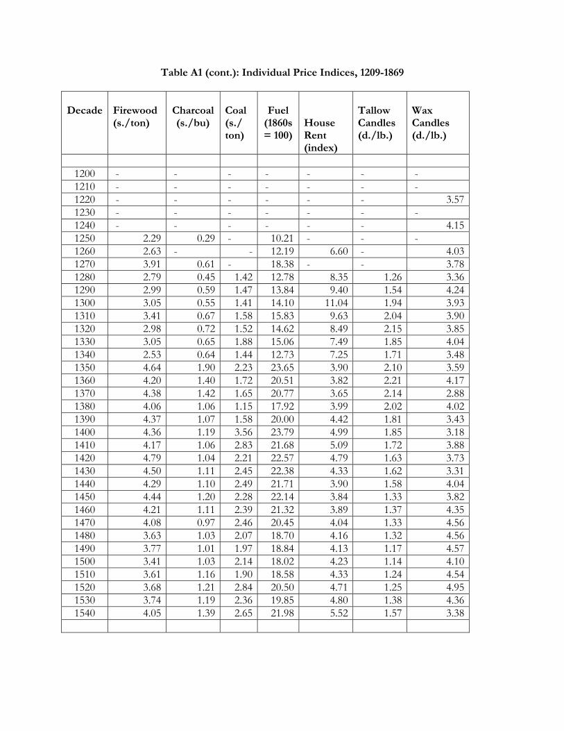
Table A1 (cont.): Individual Price Indices, 1209-1869
Decade
Firewood (s./ton)
Charcoal (s./bu)
Coal (s./ ton)
Fuel
(1860s = 100)
House Rent (index)
Tallow Candles (d./lb.)
Wax Candles (d./lb.)
1200 - - - - - - - 1210 - - - - - - - 1220 - - - - - - 3.571230 - - - - - - - 1240 - - - - - - 4.151250 2.29 0.29 - 10.21 - - - 1260 2.63 - - 12.19 6.60 - 4.031270 3.91 0.61 - 18.38 - - 3.781280 2.79 0.45 1.42 12.78 8.35 1.26 3.361290 2.99 0.59 1.47 13.84 9.40 1.54 4.241300 3.05 0.55 1.41 14.10 11.04 1.94 3.931310 3.41 0.67 1.58 15.83 9.63 2.04 3.901320 2.98 0.72 1.52 14.62 8.49 2.15 3.851330 3.05 0.65 1.88 15.06 7.49 1.85 4.041340 2.53 0.64 1.44 12.73 7.25 1.71 3.481350 4.64 1.90 2.23 23.65 3.90 2.10 3.591360 4.20 1.40 1.72 20.51 3.82 2.21 4.171370 4.38 1.42 1.65 20.77 3.65 2.14 2.881380 4.06 1.06 1.15 17.92 3.99 2.02 4.021390 4.37 1.07 1.58 20.00 4.42 1.81 3.431400 4.36 1.19 3.56 23.79 4.99 1.85 3.181410 4.17 1.06 2.83 21.68 5.09 1.72 3.881420 4.79 1.04 2.21 22.57 4.79 1.63 3.731430 4.50 1.11 2.45 22.38 4.33 1.62 3.311440 4.29 1.10 2.49 21.71 3.90 1.58 4.041450 4.44 1.20 2.28 22.14 3.84 1.33 3.821460 4.21 1.11 2.39 21.32 3.89 1.37 4.351470 4.08 0.97 2.46 20.45 4.04 1.33 4.561480 3.63 1.03 2.07 18.70 4.16 1.32 4.561490 3.77 1.01 1.97 18.84 4.13 1.17 4.571500 3.41 1.03 2.14 18.02 4.23 1.14 4.101510 3.61 1.16 1.90 18.58 4.33 1.24 4.541520 3.68 1.21 2.84 20.50 4.71 1.25 4.951530 3.74 1.19 2.36 19.85 4.80 1.38 4.361540 4.05 1.39 2.65 21.98 5.52 1.57 3.38
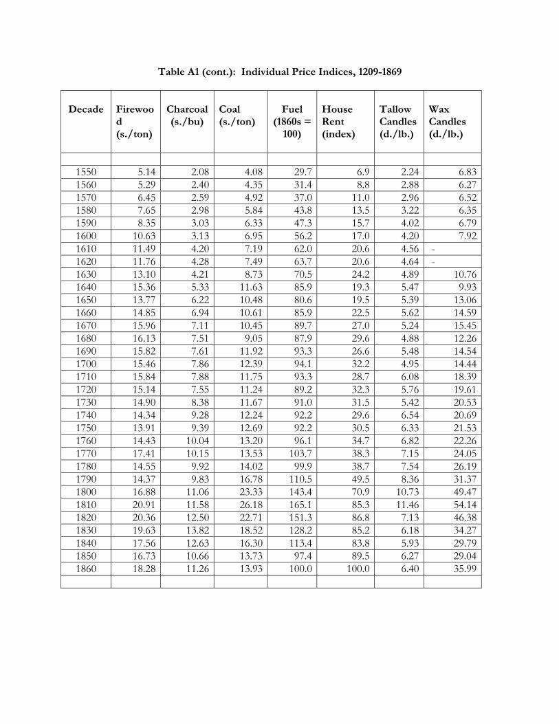
Table A1 (cont.): Individual Price Indices, 1209-1869
Decade
Firewood (s./ton)
Charcoal (s./bu)
Coal (s./ton)
Fuel
(1860s = 100)
House Rent (index)
Tallow Candles (d./lb.)
Wax Candles (d./lb.)
1550 5.14 2.08 4.08 29.7 6.9 2.24 6.831560 5.29 2.40 4.35 31.4 8.8 2.88 6.271570 6.45 2.59 4.92 37.0 11.0 2.96 6.521580 7.65 2.98 5.84 43.8 13.5 3.22 6.351590 8.35 3.03 6.33 47.3 15.7 4.02 6.791600 10.63 3.13 6.95 56.2 17.0 4.20 7.921610 11.49 4.20 7.19 62.0 20.6 4.56 - 1620 11.76 4.28 7.49 63.7 20.6 4.64 - 1630 13.10 4.21 8.73 70.5 24.2 4.89 10.761640 15.36 5.33 11.63 85.9 19.3 5.47 9.931650 13.77 6.22 10.48 80.6 19.5 5.39 13.061660 14.85 6.94 10.61 85.9 22.5 5.62 14.591670 15.96 7.11 10.45 89.7 27.0 5.24 15.451680 16.13 7.51 9.05 87.9 29.6 4.88 12.261690 15.82 7.61 11.92 93.3 26.6 5.48 14.541700 15.46 7.86 12.39 94.1 32.2 4.95 14.441710 15.84 7.88 11.75 93.3 28.7 6.08 18.391720 15.14 7.55 11.24 89.2 32.3 5.76 19.611730 14.90 8.38 11.67 91.0 31.5 5.42 20.531740 14.34 9.28 12.24 92.2 29.6 6.54 20.691750 13.91 9.39 12.69 92.2 30.5 6.33 21.531760 14.43 10.04 13.20 96.1 34.7 6.82 22.261770 17.41 10.15 13.53 103.7 38.3 7.15 24.051780 14.55 9.92 14.02 99.9 38.7 7.54 26.191790 14.37 9.83 16.78 110.5 49.5 8.36 31.371800 16.88 11.06 23.33 143.4 70.9 10.73 49.471810 20.91 11.58 26.18 165.1 85.3 11.46 54.141820 20.36 12.50 22.71 151.3 86.8 7.13 46.381830 19.63 13.82 18.52 128.2 85.2 6.18 34.271840 17.56 12.63 16.30 113.4 83.8 5.93 29.791850 16.73 10.66 13.73 97.4 89.5 6.27 29.041860 18.28 11.26 13.93 100.0 100.0 6.40 35.99
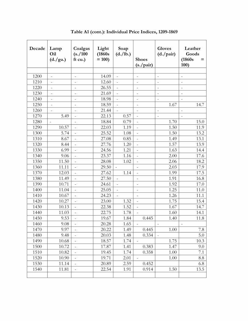
Table A1 (cont.): Individual Price Indices, 1209-1869
Decade
Lamp Oil (d./ga.)
Coalgas (s./100 ft cu.)
Light (1860s = 100)
Soap
(d./lb.)Shoes (s./pair)
Gloves (d./pair)
Leather Goods
(1860s = 100)
1200 - - 14.09 - - - - 1210 - - 12.60 - - - - 1220 - - 26.55 - - - - 1230 - - 21.69 - - - - 1240 - - 18.98 - - - - 1250 - - 18.59 - - 1.67 14.71260 - - 21.44 - - - - 1270 5.49 - 22.13 0.57 - - - 1280 - - 18.84 0.79 - 1.70 15.01290 10.57 - 22.03 1.19 - 1.50 11.91300 5.74 - 25.52 1.08 - 1.50 13.21310 8.67 - 27.08 0.85 - 1.49 13.11320 8.44 - 27.76 1.20 - 1.57 13.91330 6.99 - 24.56 1.21 - 1.63 14.41340 9.06 - 23.37 1.16 - 2.00 17.61350 11.50 - 28.08 1.02 - 2.06 18.21360 11.11 - 29.50 - - 2.03 17.91370 12.03 - 27.62 1.14 - 1.99 17.51380 11.49 - 27.50 - - 1.91 16.81390 10.71 - 24.61 - - 1.92 17.01400 11.04 - 25.05 - - 1.25 11.01410 10.67 - 24.23 - - 1.26 11.11420 10.27 - 23.00 1.32 - 1.75 15.41430 10.13 - 22.38 1.52 - 1.67 14.71440 11.03 - 22.75 1.78 - 1.60 14.11450 9.53 - 19.67 1.84 0.445 1.40 11.81460 9.08 - 20.28 1.65 - - - 1470 9.97 - 20.22 1.49 0.445 1.00 7.81480 9.48 - 20.03 1.48 0.334 - 5.01490 10.68 - 18.57 1.74 - 1.75 10.31500 10.72 - 17.87 1.41 0.383 1.47 9.01510 10.82 - 19.45 1.74 0.358 1.00 7.11520 10.90 - 19.71 2.01 - 1.00 8.81530 11.14 - 20.89 2.59 0.452 6.81540 11.81 - 22.54 1.91 0.914 1.50 13.5
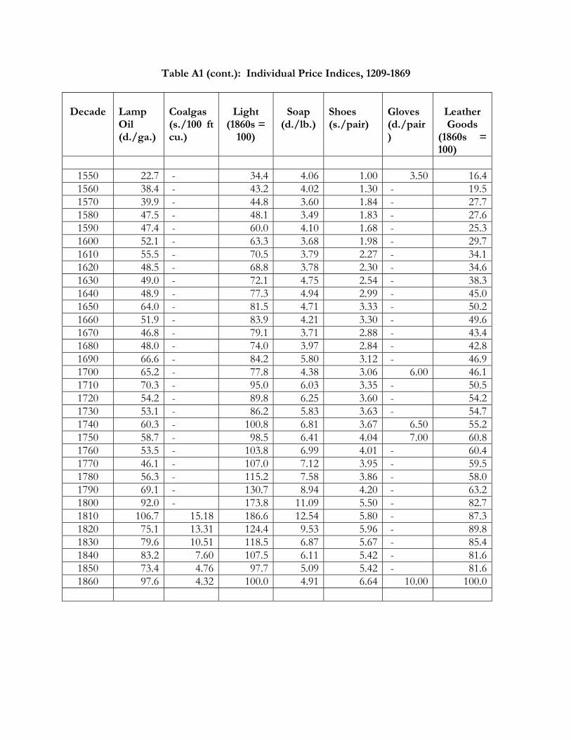
Table A1 (cont.): Individual Price Indices, 1209-1869
Decade
Lamp Oil (d./ga.)
Coalgas (s./100 ft cu.)
Light
(1860s = 100)
Soap
(d./lb.)
Shoes (s./pair)
Gloves (d./pair)
Leather Goods
(1860s = 100)
1550 22.7 - 34.4 4.06 1.00 3.50 16.41560 38.4 - 43.2 4.02 1.30 - 19.51570 39.9 - 44.8 3.60 1.84 - 27.71580 47.5 - 48.1 3.49 1.83 - 27.61590 47.4 - 60.0 4.10 1.68 - 25.31600 52.1 - 63.3 3.68 1.98 - 29.71610 55.5 - 70.5 3.79 2.27 - 34.11620 48.5 - 68.8 3.78 2.30 - 34.61630 49.0 - 72.1 4.75 2.54 - 38.31640 48.9 - 77.3 4.94 2.99 - 45.01650 64.0 - 81.5 4.71 3.33 - 50.21660 51.9 - 83.9 4.21 3.30 - 49.61670 46.8 - 79.1 3.71 2.88 - 43.41680 48.0 - 74.0 3.97 2.84 - 42.81690 66.6 - 84.2 5.80 3.12 - 46.91700 65.2 - 77.8 4.38 3.06 6.00 46.11710 70.3 - 95.0 6.03 3.35 - 50.51720 54.2 - 89.8 6.25 3.60 - 54.21730 53.1 - 86.2 5.83 3.63 - 54.71740 60.3 - 100.8 6.81 3.67 6.50 55.21750 58.7 - 98.5 6.41 4.04 7.00 60.81760 53.5 - 103.8 6.99 4.01 - 60.41770 46.1 - 107.0 7.12 3.95 - 59.51780 56.3 - 115.2 7.58 3.86 - 58.01790 69.1 - 130.7 8.94 4.20 - 63.21800 92.0 - 173.8 11.09 5.50 - 82.71810 106.7 15.18 186.6 12.54 5.80 - 87.31820 75.1 13.31 124.4 9.53 5.96 - 89.81830 79.6 10.51 118.5 6.87 5.67 - 85.41840 83.2 7.60 107.5 6.11 5.42 - 81.61850 73.4 4.76 97.7 5.09 5.42 - 81.61860 97.6 4.32 100.0 4.91 6.64 10.00 100.0
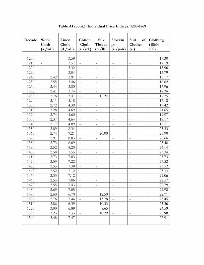
Table A1 (cont.): Individual Price Indices, 1209-1869
Decade
Wool Cloth (s./yd.)
Linen Cloth (d./yd.)
Cotton Cloth
(s./yd.)
Silk
Thread (d./lb.)
Stockings (s./pair)
Suit of Clothes (s.)
Clothing (1860s = 100)
1200 - 3.59 - - - - 17.301210 - 3.57 - - - - 17.191220 - 3.32 - - - - 15.961230 - 3.04 - - - - 14.791240 2.42 3.91 - - - - 18.171250 2.55 3.46 - - - - 16.621260 2.44 3.80 - - - - 17.961270 2.41 3.74 - - - - 17.361280 2.76 3.47 - 12.24 - - 17.751290 2.11 4.18 - - - - 17.181300 2.72 4.39 - - - - 19.421310 3.28 4.69 - - - - 21.651320 2.74 4.60 - - - - 19.971330 2.37 4.64 - - - - 18.171340 2.17 4.09 - - - - 16.511350 2.89 8.34 - - - - 25.331360 2.74 9.21 - 20.00 - - 25.901370 2.91 8.83 - - - - 26.661380 2.73 8.69 - - - - 25.481390 2.52 8.20 - - - - 24.141400 2.58 7.55 - - - - 23.341410 2.73 7.03 - - - - 23.731420 2.59 7.22 - - - - 23.521430 2.55 7.38 - - - - 23.521440 2.52 7.12 - - - - 23.341450 2.33 7.12 - - - - 22.061460 2.55 7.06 - - - - 22.571470 2.55 7.43 - - - - 22.791480 2.69 7.05 - - - - 22.981490 2.60 6.70 - 12.50 - - 22.711500 2.76 7.44 - 13.78 - - 23.451510 2.86 6.39 - 10.33 - - 23.361520 3.00 6.89 - 8.65 - - 24.591530 3.23 7.33 - 10.29 - - 25.981540 3.48 7.47 - - - - 27.91
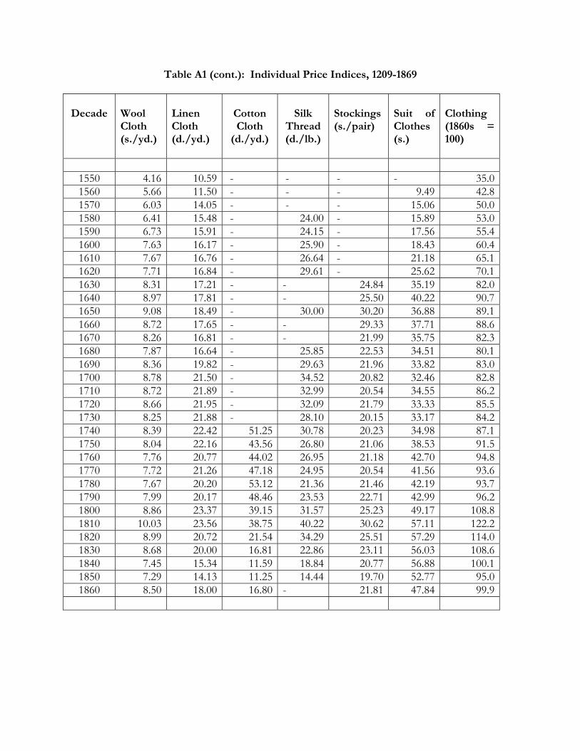
Table A1 (cont.): Individual Price Indices, 1209-1869
Decade
Wool Cloth (s./yd.)
Linen Cloth (d./yd.)
Cotton Cloth
(d./yd.)
Silk
Thread (d./lb.)
Stockings (s./pair)
Suit of Clothes (s.)
Clothing (1860s = 100)
1550 4.16 10.59 - - - - 35.01560 5.66 11.50 - - - 9.49 42.81570 6.03 14.05 - - - 15.06 50.01580 6.41 15.48 - 24.00 - 15.89 53.01590 6.73 15.91 - 24.15 - 17.56 55.41600 7.63 16.17 - 25.90 - 18.43 60.41610 7.67 16.76 - 26.64 - 21.18 65.11620 7.71 16.84 - 29.61 - 25.62 70.11630 8.31 17.21 - - 24.84 35.19 82.01640 8.97 17.81 - - 25.50 40.22 90.71650 9.08 18.49 - 30.00 30.20 36.88 89.11660 8.72 17.65 - - 29.33 37.71 88.61670 8.26 16.81 - - 21.99 35.75 82.31680 7.87 16.64 - 25.85 22.53 34.51 80.11690 8.36 19.82 - 29.63 21.96 33.82 83.01700 8.78 21.50 - 34.52 20.82 32.46 82.81710 8.72 21.89 - 32.99 20.54 34.55 86.21720 8.66 21.95 - 32.09 21.79 33.33 85.51730 8.25 21.88 - 28.10 20.15 33.17 84.21740 8.39 22.42 51.25 30.78 20.23 34.98 87.11750 8.04 22.16 43.56 26.80 21.06 38.53 91.51760 7.76 20.77 44.02 26.95 21.18 42.70 94.81770 7.72 21.26 47.18 24.95 20.54 41.56 93.61780 7.67 20.20 53.12 21.36 21.46 42.19 93.71790 7.99 20.17 48.46 23.53 22.71 42.99 96.21800 8.86 23.37 39.15 31.57 25.23 49.17 108.81810 10.03 23.56 38.75 40.22 30.62 57.11 122.21820 8.99 20.72 21.54 34.29 25.51 57.29 114.01830 8.68 20.00 16.81 22.86 23.11 56.03 108.61840 7.45 15.34 11.59 18.84 20.77 56.88 100.11850 7.29 14.13 11.25 14.44 19.70 52.77 95.01860 8.50 18.00 16.80 - 21.81 47.84 99.9

Table A1 (cont.): Individual Price Indices, 1209-1869
Decade
Tobacco(d./lb)
Books (s./ book)
Silver
(d./oz)
Pewter (d./lb)
Brass Goods (d./lb )
Woodwares (index)
Pottery (d./plate)
1200 - - 23.8 - - - - 1210 - - 23.8 - - - - 1220 - - 23.8 1.85 - - - 1230 - - 23.8 - - - - 1240 - - 23.8 - - - - 1250 - - 23.8 - - - - 1260 - - 23.8 1.79 - - - 1270 - - 23.8 1.70 2.50 - - 1280 - - 23.9 2.31 2.29 - - 1290 - - 23.9 2.17 2.28 - - 1300 - - 23.9 2.20 2.00 - - 1310 - - 23.9 2.89 3.00 - - 1320 - - 23.9 2.64 2.53 - - 1330 - - 24.3 2.64 3.05 - - 1340 - - 25.6 2.51 2.46 - - 1350 - - 29.2 3.34 2.87 - - 1360 - - 29.5 3.55 3.01 - - 1370 - - 29.5 3.48 3.43 - - 1380 - - 29.5 3.43 3.84 - - 1390 - - 29.5 3.18 3.77 - - 1400 - - 29.5 3.47 3.93 - - 1410 - - 34.2 3.30 3.61 - - 1420 - - 35.4 2.87 3.00 - - 1430 - - 35.4 2.75 3.10 - - 1440 - - 35.4 3.12 4.02 - - 1450 - - 35.4 3.12 3.46 - - 1460 - - 39.8 3.17 3.79 - - 1470 - - 44.3 3.69 3.99 - - 1480 - - 44.3 3.58 3.19 - - 1490 - - 44.3 3.88 4.13 - - 1500 - - 44.3 4.24 3.87 - - 1510 - - 44.3 5.13 4.06 - - 1520 - - 47.6 4.97 3.74 - - 1530 - - 49.8 4.87 3.61 - - 1540 - - 52.5 5.26 4.51 - -
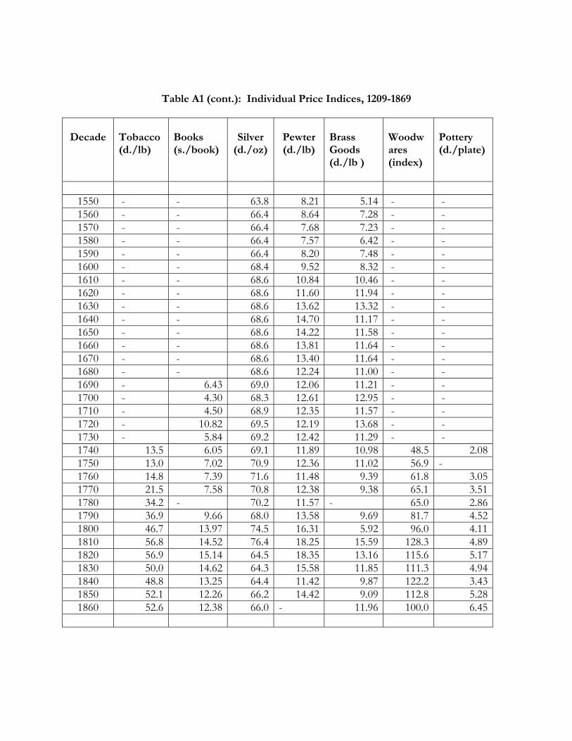
Table A1 (cont.): Individual Price Indices, 1209-1869
Decade
Tobacco(d./lb)
Books (s./book)
Silver
(d./oz)
Pewter (d./lb)
Brass Goods (d./lb )
Woodwares (index)
Pottery (d./plate)
1550 - - 63.8 8.21 5.14 - - 1560 - - 66.4 8.64 7.28 - - 1570 - - 66.4 7.68 7.23 - - 1580 - - 66.4 7.57 6.42 - - 1590 - - 66.4 8.20 7.48 - - 1600 - - 68.4 9.52 8.32 - - 1610 - - 68.6 10.84 10.46 - - 1620 - - 68.6 11.60 11.94 - - 1630 - - 68.6 13.62 13.32 - - 1640 - - 68.6 14.70 11.17 - - 1650 - - 68.6 14.22 11.58 - - 1660 - - 68.6 13.81 11.64 - - 1670 - - 68.6 13.40 11.64 - - 1680 - - 68.6 12.24 11.00 - - 1690 - 6.43 69.0 12.06 11.21 - - 1700 - 4.30 68.3 12.61 12.95 - - 1710 - 4.50 68.9 12.35 11.57 - - 1720 - 10.82 69.5 12.19 13.68 - - 1730 - 5.84 69.2 12.42 11.29 - - 1740 13.5 6.05 69.1 11.89 10.98 48.5 2.081750 13.0 7.02 70.9 12.36 11.02 56.9 - 1760 14.8 7.39 71.6 11.48 9.39 61.8 3.051770 21.5 7.58 70.8 12.38 9.38 65.1 3.511780 34.2 - 70.2 11.57 - 65.0 2.861790 36.9 9.66 68.0 13.58 9.69 81.7 4.521800 46.7 13.97 74.5 16.31 5.92 96.0 4.111810 56.8 14.52 76.4 18.25 15.59 128.3 4.891820 56.9 15.14 64.5 18.35 13.16 115.6 5.171830 50.0 14.62 64.3 15.58 11.85 111.3 4.941840 48.8 13.25 64.4 11.42 9.87 122.2 3.431850 52.1 12.26 66.2 14.42 9.09 112.8 5.281860 52.6 12.38 66.0 - 11.96 100.0 6.45
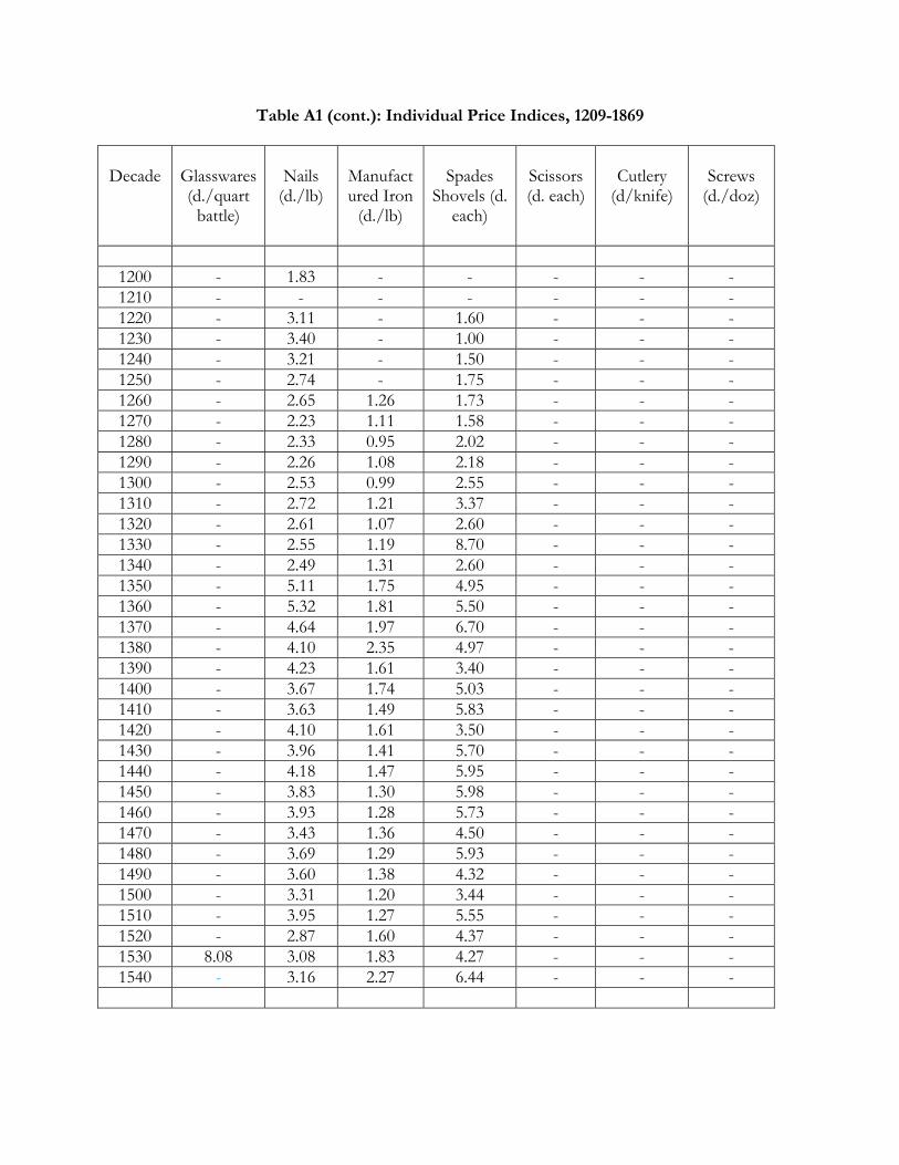
Table A1 (cont.): Individual Price Indices, 1209-1869
Decade
Glasswares (d./quart
battle)
Nails
(d./lb)
Manufactured Iron
(d./lb)
Spades
Shovels (d. each)
Scissors (d. each)
Cutlery
(d/knife)
Screws
(d./doz)
1200 - 1.83 - - - - - 1210 - - - - - - - 1220 - 3.11 - 1.60 - - - 1230 - 3.40 - 1.00 - - - 1240 - 3.21 - 1.50 - - - 1250 - 2.74 - 1.75 - - - 1260 - 2.65 1.26 1.73 - - - 1270 - 2.23 1.11 1.58 - - - 1280 - 2.33 0.95 2.02 - - - 1290 - 2.26 1.08 2.18 - - - 1300 - 2.53 0.99 2.55 - - - 1310 - 2.72 1.21 3.37 - - - 1320 - 2.61 1.07 2.60 - - - 1330 - 2.55 1.19 8.70 - - - 1340 - 2.49 1.31 2.60 - - - 1350 - 5.11 1.75 4.95 - - - 1360 - 5.32 1.81 5.50 - - - 1370 - 4.64 1.97 6.70 - - - 1380 - 4.10 2.35 4.97 - - - 1390 - 4.23 1.61 3.40 - - - 1400 - 3.67 1.74 5.03 - - - 1410 - 3.63 1.49 5.83 - - - 1420 - 4.10 1.61 3.50 - - - 1430 - 3.96 1.41 5.70 - - - 1440 - 4.18 1.47 5.95 - - - 1450 - 3.83 1.30 5.98 - - - 1460 - 3.93 1.28 5.73 - - - 1470 - 3.43 1.36 4.50 - - - 1480 - 3.69 1.29 5.93 - - - 1490 - 3.60 1.38 4.32 - - - 1500 - 3.31 1.20 3.44 - - - 1510 - 3.95 1.27 5.55 - - - 1520 - 2.87 1.60 4.37 - - - 1530 8.08 3.08 1.83 4.27 - - - 1540 - 3.16 2.27 6.44 - - -
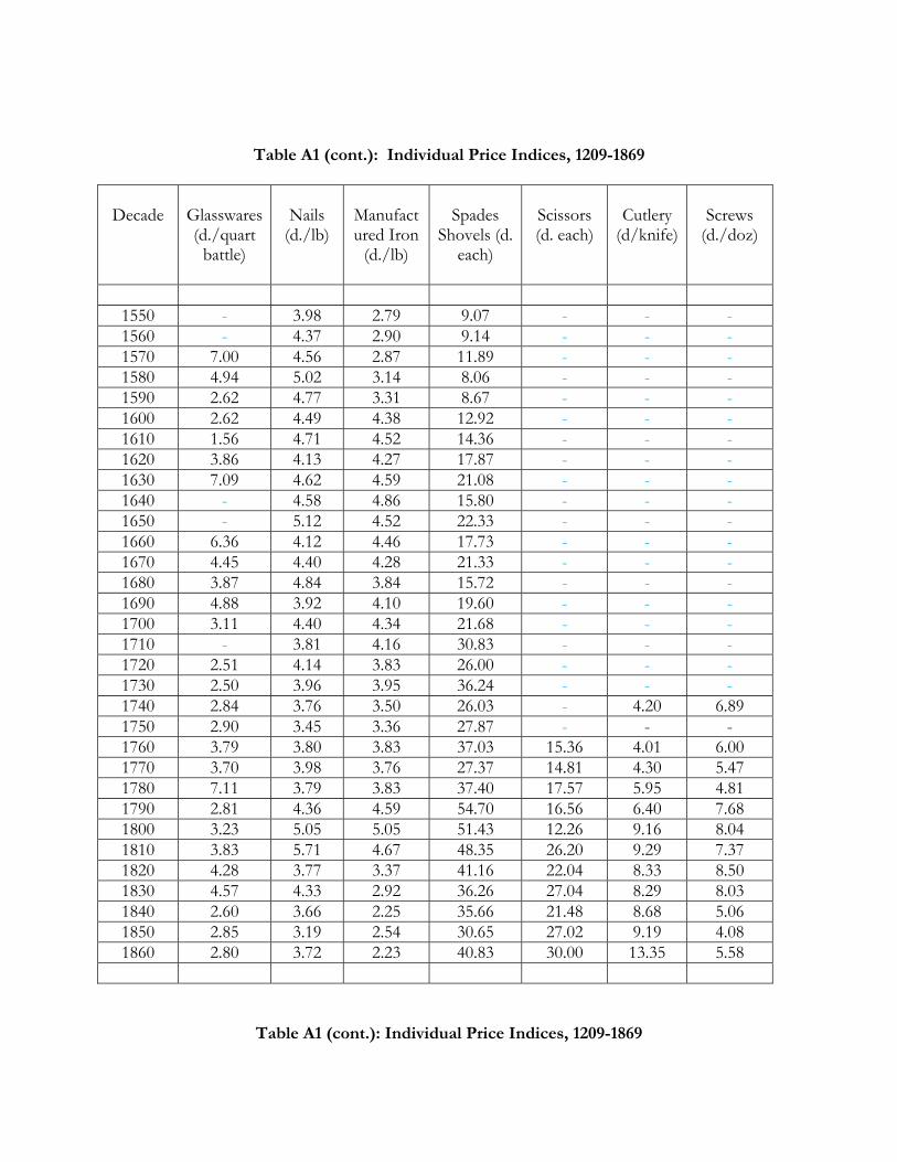
Table A1 (cont.): Individual Price Indices, 1209-1869
Decade
Glasswares (d./quart
battle)
Nails
(d./lb)
Manufactured Iron
(d./lb)
Spades
Shovels (d. each)
Scissors (d. each)
Cutlery
(d/knife)
Screws
(d./doz)
1550 - 3.98 2.79 9.07 - - - 1560 - 4.37 2.90 9.14 - - - 1570 7.00 4.56 2.87 11.89 - - - 1580 4.94 5.02 3.14 8.06 - - - 1590 2.62 4.77 3.31 8.67 - - - 1600 2.62 4.49 4.38 12.92 - - - 1610 1.56 4.71 4.52 14.36 - - - 1620 3.86 4.13 4.27 17.87 - - - 1630 7.09 4.62 4.59 21.08 - - - 1640 - 4.58 4.86 15.80 - - - 1650 - 5.12 4.52 22.33 - - - 1660 6.36 4.12 4.46 17.73 - - - 1670 4.45 4.40 4.28 21.33 - - - 1680 3.87 4.84 3.84 15.72 - - - 1690 4.88 3.92 4.10 19.60 - - - 1700 3.11 4.40 4.34 21.68 - - - 1710 - 3.81 4.16 30.83 - - - 1720 2.51 4.14 3.83 26.00 - - - 1730 2.50 3.96 3.95 36.24 - - - 1740 2.84 3.76 3.50 26.03 - 4.20 6.89 1750 2.90 3.45 3.36 27.87 - - - 1760 3.79 3.80 3.83 37.03 15.36 4.01 6.00 1770 3.70 3.98 3.76 27.37 14.81 4.30 5.47 1780 7.11 3.79 3.83 37.40 17.57 5.95 4.81 1790 2.81 4.36 4.59 54.70 16.56 6.40 7.68 1800 3.23 5.05 5.05 51.43 12.26 9.16 8.04 1810 3.83 5.71 4.67 48.35 26.20 9.29 7.37 1820 4.28 3.77 3.37 41.16 22.04 8.33 8.50 1830 4.57 4.33 2.92 36.26 27.04 8.29 8.03 1840 2.60 3.66 2.25 35.66 21.48 8.68 5.06 1850 2.85 3.19 2.54 30.65 27.02 9.19 4.08 1860 2.80 3.72 2.23 40.83 30.00 13.35 5.58
Table A1 (cont.): Individual Price Indices, 1209-1869
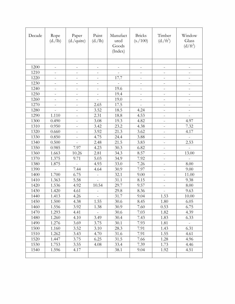
Decade
Rope (d./lb)
Paper
(d./quire)
Paint
(d./lb)
Manufact
ured Goods (Index)
Bricks
(s./100)
Timber (d./ft3)
Window
Glass (d/ft2)
1200 - - - - - - - 1210 - - - - - - - 1220 - - - 17.7 - - - 1230 - - - - - - - 1240 - - - 19.6 - - - 1250 - - - 19.4 - - - 1260 - - - 19.0 - - - 1270 - - 2.65 17.5 - - - 1280 - - 3.52 18.5 4.24 - - 1290 1.110 - 2.31 18.8 4.53 - - 1300 0.490 - 3.08 19.3 4.82 - 4.97 1310 0.950 - 3.42 23.2 4.38 - 7.32 1320 0.660 - 3.92 21.3 3.62 - 4.17 1330 0.850 - 4.75 24.4 3.88 - - 1340 0.500 - 2.48 21.5 3.83 - 2.53 1350 0.985 7.97 4.23 30.3 6.82 - - 1360 1.663 10.26 2.81 34.3 8.57 - 13.00 1370 1.375 9.71 5.03 34.9 7.92 - - 1380 1.875 - 4.93 33.0 7.26 - 8.00 1390 - 7.44 4.64 30.9 7.97 - 9.00 1400 1.700 6.75 - 32.1 9.00 - 11.00 1410 1.363 5.58 - 31.1 8.15 - 9.38 1420 1.536 4.92 10.54 29.7 9.57 - 8.00 1430 1.420 4.61 - 29.8 8.36 - 9.63 1440 1.413 4.26 - 31.7 9.04 1.53 10.00 1450 1.500 4.38 1.55 30.6 8.45 1.80 6.05 1460 1.556 3.92 1.38 30.9 7.60 0.53 6.75 1470 1.293 4.41 - 30.6 7.03 1.82 4.39 1480 1.260 4.10 3.49 30.4 7.43 1.83 6.33 1490 1.276 3.69 3.75 30.1 7.93 1.81 - 1500 1.160 3.52 3.10 28.3 7.91 1.43 6.31 1510 1.262 3.43 4.70 31.6 7.91 1.55 4.61 1520 1.447 3.75 6.25 31.5 7.66 1.28 4.96 1530 1.753 3.55 4.08 33.4 7.39 1.73 4.46 1540 1.596 4.17 38.1 9.04 1.92 4.51
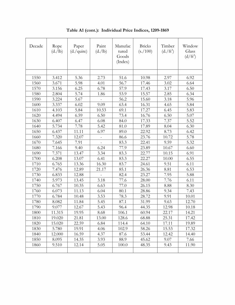
Table A1 (cont.): Individual Price Indices, 1209-1869
Decade
Rope (d./lb)
Paper
(d./quire)
Paint
(d./lb)
Manufac
tured Goods (Index)
Bricks
(s./100)
Timber (d./ft3)
Window
Glass (d/ft2)
1550 3.412 5.36 2.73 51.6 10.98 2.97 6.92 1560 3.671 5.98 4.01 56.7 17.46 3.02 6.64 1570 3.156 6.25 6.78 57.9 17.43 3.17 6.50 1580 2.804 5.74 1.86 53.9 15.57 2.85 6.34 1590 3.224 5.67 - 56.2 15.60 3.18 5.96 1600 3.337 6.02 9.09 63.4 16.31 4.65 5.84 1610 4.103 5.84 10.53 69.1 17.27 6.45 5.83 1620 4.494 6.59 6.50 73.4 16.76 6.50 5.07 1630 6.407 6.47 6.08 84.0 17.33 7.37 5.52 1640 5.734 7.78 5.42 81.0 17.89 8.04 6.30 1650 6.437 11.11 6.97 89.0 22.92 8.73 6.42 1660 7.320 12.07 - 86.6 23.76 10.72 5.78 1670 7.645 7.91 - 83.3 22.41 9.59 5.32 1680 7.166 9.40 6.24 77.9 23.89 10.67 6.60 1690 7.371 13.47 3.34 83.3 22.77 10.15 6.91 1700 6.208 13.07 6.41 83.3 22.27 10.00 6.55 1710 6.765 13.36 16.30 83.7 24.61 9.51 6.11 1720 7.476 12.89 21.17 85.1 26.36 8.81 6.53 1730 6.833 12.88 - 82.4 23.27 7.95 5.88 1740 5.973 13.45 3.18 77.6 28.00 7.76 6.11 1750 6.767 10.35 6.63 77.0 26.15 8.88 8.30 1760 6.073 11.13 6.04 80.1 28.86 9.34 7.43 1770 6.784 10.48 3.53 78.3 28.72 9.91 10.01 1780 8.082 11.84 5.45 87.1 31.99 9.63 12.70 1790 9.077 12.67 5.43 96.4 44.35 12.98 10.18 1800 11.315 19.95 8.68 106.1 60.94 22.17 14.21 1810 19.020 21.81 13.00 128.6 68.88 25.31 17.42 1820 15.020 22.59 6.84 114.4 64.10 17.11 19.89 1830 5.780 19.91 4.06 102.9 58.26 15.53 17.32 1840 12.000 16.59 4.37 87.6 53.44 12.42 14.40 1850 8.095 14.35 3.93 88.9 45.62 9.07 7.66 1860 9.510 12.14 5.05 100.0 48.35 9.43 11.90