the kuramoto model with inertia: from fireflies to power grids
TRANSCRIPT
The Kuramoto model with inertia: from fireflies to
power grids
Simona Olmi
Inria Sophia Antipolis Mediterranee Research Centre - Sophia Antipolis, France
Istituto dei Sistemi Complessi - CNR - Firenze, Italy
Patterns of Synchrony: Chimera States and Beyond – p. 1
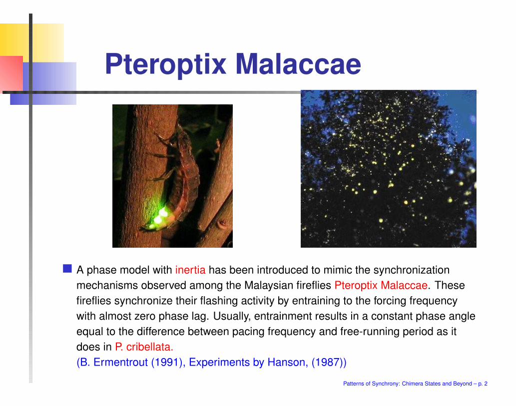
Pteroptix Malaccae
A phase model with inertia has been introduced to mimic the synchronization
mechanisms observed among the Malaysian fireflies Pteroptix Malaccae. These
fireflies synchronize their flashing activity by entraining to the forcing frequency
with almost zero phase lag. Usually, entrainment results in a constant phase angle
equal to the difference between pacing frequency and free-running period as it
does in P. cribellata.
(B. Ermentrout (1991), Experiments by Hanson, (1987))
Patterns of Synchrony: Chimera States and Beyond – p. 2

Why introducing “inertia”?
First-order Kuramoto model
It approaches too fast the partial synchronized state
Infinite coupling strength is required to achive full synchronization
Second-order Kuramoto model
Synchronization is slowed down by inertia (frequency adaptation)
Firstly proposed in biological context (Ermentrout, (1991))
Used to study synchronization in disordered arrays of Josephson junctions
(Strogatz (1994), Trees et al. (2005))
Derived from the classical swing equation to study synchronization in power
grids (Filatrella et al. (2008))
Patterns of Synchrony: Chimera States and Beyond – p. 3
The Model
Kuramoto model with inertia
mθi + θi = Ωi +K
N
∑
j
sin(θj − θi)
θi is the instantaneous phase
Ωi is the natural frequency of the i−th oscillator with Gaussian distribution
K is the coupling constant
N is the number of oscillators
By introducing the complex order parameter r(t)eiφ(t) = 1N
∑
j eiθj
mθi + θi = Ωi −Kr sin(θi − φ)
r = 0 asynchronous state, r = 1 synchronized state
Patterns of Synchrony: Chimera States and Beyond – p. 4

Damped Driven Pendulum
mθi + θi = Ωi −Kr sin(θi)
I = Ωi
Kr
β = 1√mKr
φ+ βφ = I − sin(φ)
One node connected to the grid (the grid is considered to be infinite)
Single damped driven pendulum
Josephson junctions
One-machine infinite bus system of a generator in a power-grid (Chiang, (2011))
Patterns of Synchrony: Chimera States and Beyond – p. 5

Damped Driven Pendulum
φ + βφ = I − sin(φ)
For sufficiently large m (small β)
For small Ωi two fixed points are
present: a stable node and a saddle.
The linear stability is given by
J =
0 1
− cosφ∗ −β
σ1,2 =−β±
√β2−4 cosφ∗
2
At large frequencies Ωi > ΩP =4π
√
Krm
(i.e. I > 4βπ
) a limit cycle
emerges from the saddle via a homo-
clinic bifurcation
Limit cycle and fixed point coexists until Ωi ≡ ΩD = Kr (i.e. I = 1), where a
saddle node bifurcation leads to the disappearence of the two fixed points
For Ωi > ΩD (i.e. I > 1) only the oscillating solution is present
For small mass (large β), there is no more coexistence.
(Levi et al. 1978) Patterns of Synchrony: Chimera States and Beyond – p. 6

Simulation ProtocolsDynamics of N oscillators (first order transition and hysteresis)
ΩM maximal natural frequency of the locked oscillators
Ω(I)P = 4
π
√
Krm
Ω(II)D = Kr
Protocol I: Increasing K
The system remains desynchronized
until K = K1c (filled black circles).
ΩM increases with K following ΩIP .
Ωi are grouped in small clusters
(plateaus).
Protocol II: Decreasing K
The system remains synchronized until
K = K2c (empty black circles).
ΩM remains stucked to the same value
for a large K interval than it rapidly de-
creases to 0 following ΩIID .
0
1
2
3
0 2 4 6 8 10
K
0
0.5
1
ΩM
ΩM
ΩP
(I)
ΩD
(II)
r
K1
c
K2
c
Protocol I
Protocol II
m = 2
Patterns of Synchrony: Chimera States and Beyond – p. 7
Mean Field Theory
(Tanaka et al. (1997))
mθi + θi = Ωi −Kr sin(θi − φ)
by following Protocol I and II there is a group of drifting oscillators and one of
locked oscillators which act separately
locked oscillators are characterized by < θ >= 0 and are locked to the mean
phase
drifting oscillators (with < θ > 6= 0) are whirling over the locked subgroup (or
below depending on the sign of Ωi)
Drifting and locked oscillators are separated by a certain frequency:
Following Protocol I the oscillators with Ωi < ΩP are locked
Following Protocol II the oscillators with Ωi < ΩD are locked
These two groups contribute differently to the total level of synchronization in the
system
r = rL + rD
Patterns of Synchrony: Chimera States and Beyond – p. 8
Mean Field Theory
(Tanaka et al. (1997))
Protocol I: Ω(I)P = 4
π
√
Krm
All oscillators initially drift around its own natural frequency Ωi
Increasing K, oscillators with Ωi < ΩP are attracted by the locked group
Increasing K also ΩP increases ⇒ oscillators with bigger Ωi become
synchronized
The phase coherence rI increases and Ωi exhibits plateaus
! Depending on m the transition to synchronization may increase in complexity
Protocol II: Ω(II)D = Kr
Oscillators are initially locked to the mean phase and rII ≈ 1
Decreasing K, locked oscillators are desynchronized and start whirling when
Ωi > ΩD and a saddle node bifurcation occurs
ΩP , ΩD are the synchronization boundaries
Patterns of Synchrony: Chimera States and Beyond – p. 9

Mean Field Theory
(Tanaka et al. (1997))
Total level of synchronization in the system: r = rL + rD
For the locked population the self-consistent equation is
rI,IIL = Kr
∫ θP,D
−θP,D
cos2 θ g(Kr sin θ)dθ
where θP = sin−1(ΩP
Kr), θD = sin−1(ΩD
Kr) = π/2, g(Ω) frequency distribution.
The drifting population contributes to the total order parameter with a negative
contribution
rI,IID ≃ −mKr
∫ ∞
−ΩP,D
1
(mΩ)3g(Ω)dΩ
The former equation are correct in the limit of sufficiently large masses
Patterns of Synchrony: Chimera States and Beyond – p. 10

Hysteretic Behavior
Numerical Results for Fully Coupled Networks (N = 500, m = 6)
The data obtained by following protocol II are quite well reproduced by the mean
field approximation rII
The mean field extimation rI does not reproduce the stepwise structure
numerically obtained in protocol I
Clusters of NL locked oscillators of
any size remain stable between rI
and rII
The level of synchronization of these
clusters can be theoretically obtained
by generalizing the theory of Tanaka
et al. (1997) to protocols where ΩM
remains constant
(Olmi et al. (2014))0 2 4 6 8 10 12 14 16 18 20
K
0
0.2
0.4
0.6
0.8
1
r
0 5 10 15 20
K0
100
200
300
400
500
NL
Patterns of Synchrony: Chimera States and Beyond – p. 11
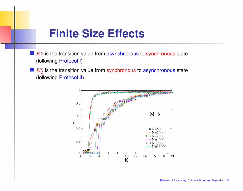
Finite Size Effects
Kc1 is the transition value from asynchronous to synchronous state
(following Protocol I)
Kc2 is the transition value from synchronous to asynchronous state
(following Protocol II)
0 2 4 6 8 10 12 14 16 18 20
K
0
0.2
0.4
0.6
0.8
1
r
N=500N=1000N=2000N=4000N=8000 N=16000
M=6
Patterns of Synchrony: Chimera States and Beyond – p. 12
Finite Size Effects
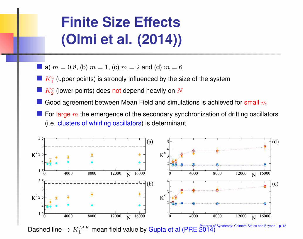
(Olmi et al. (2014))
a) m = 0.8, (b) m = 1, (c) m = 2 and (d) m = 6
Kc1 (upper points) is strongly influenced by the size of the system
Kc2 (lower points) does not depend heavily on N
Good agreement between Mean Field and simulations is achieved for small m
For large m the emergence of the secondary synchronization of drifting oscillators
(i.e. clusters of whirling oscillators) is determinant
Dashed line → KMF1 mean field value by Gupta et al (PRE 2014)
Patterns of Synchrony: Chimera States and Beyond – p. 13

Drifting Clusters
For larger masses (m=6), the synchronization transition becomes more complex, it
occurs via the emergence of clusters of drifting oscillators.
The partially synchronized state is characterized by the coexistence of
a cluster of locked oscillators with < θ >≃ 0
clusters composed by drifting oscillators with finite average velocities
Extra clusters induce (periodic or quasi-periodic) oscillations in the temporal evolution of
r(t).
0 20 40 60 80
time
0
0.2
0.4
0.6
0.8
1
r(t)
(b)
(Olmi et al. (2014))Patterns of Synchrony: Chimera States and Beyond – p. 14

Drifting Clusters
If we compare the evolution of the instantaneous velocities θi for 3 oscillators and r(t)
we observe that
the phase velocities of O2 and O3 display synchronized motion
the phase velocity of O1 oscillates irregularly around zero
the oscillations of r(t) are driven by the periodic oscillations of O2 and O3
0 10 20 30 40
time
0
0.5
1
1.5
2
r(t) O1
O3
O2
(b)
(Olmi et al. (2014)) Patterns of Synchrony: Chimera States and Beyond – p. 15
Linear Stability Analysis of the
Asynchronous State
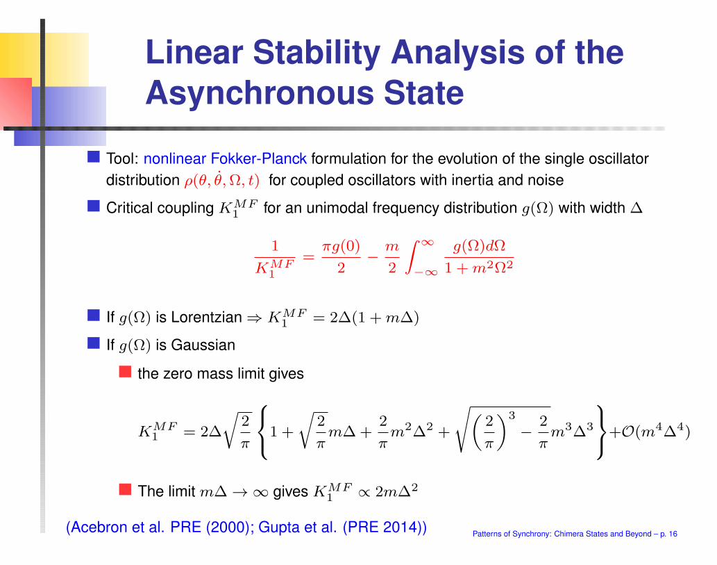
Tool: nonlinear Fokker-Planck formulation for the evolution of the single oscillator
distribution ρ(θ, θ,Ω, t) for coupled oscillators with inertia and noise
Critical coupling KMF1 for an unimodal frequency distribution g(Ω) with width ∆
1
KMF1
=πg(0)
2− m
2
∫ ∞
−∞
g(Ω)dΩ
1 +m2Ω2
If g(Ω) is Lorentzian ⇒ KMF1 = 2∆(1 +m∆)
If g(Ω) is Gaussian
the zero mass limit gives
KMF1 = 2∆
√
2
π
1 +
√
2
πm∆+
2
πm2∆2 +
√
(
2
π
)3
− 2
πm3∆3
+O(m4∆4)
The limit m∆ → ∞ gives KMF1 ∝ 2m∆2
(Acebron et al. PRE (2000); Gupta et al. (PRE 2014))Patterns of Synchrony: Chimera States and Beyond – p. 16
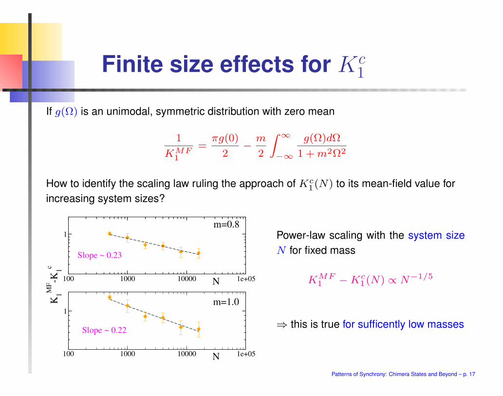
Finite size effects for Kc1
If g(Ω) is an unimodal, symmetric distribution with zero mean
1
KMF1
=πg(0)
2− m
2
∫ ∞
−∞
g(Ω)dΩ
1 +m2Ω2
How to identify the scaling law ruling the approach of Kc1(N) to its mean-field value for
increasing system sizes?
100 1000 10000 1e+05N
1
K1
MF-K
1
c
100 1000 10000 1e+05N
1
m=0.8
m=1.0
Slope ~ 0.23
Slope ~ 0.22
Power-law scaling with the system size
N for fixed mass
KMF1 −Kc
1(N) ∝ N−1/5
⇒ this is true for sufficently low masses
Patterns of Synchrony: Chimera States and Beyond – p. 17

Mean Field Theory with Noise
(Acebrón, Spigler (2008))
ξi independent sources of Gaussian white noise
θi = νi
mνi = −νi +Ωi +Kr sin(φ− θi) + ξi
with < ξi >= 0 and < ξi(t)ξj(t) >= 2Dδijδ(t− s)
Continuum limit (continuity equation for ρ(θ, ν,Ω, t))
∂ρ
∂t=
D
m2
∂2
∂ν2− 1
m
∂
∂ν[(−ν +Ω+Kr sin(φ− θ))ρ]− ν
∂ρ
∂θ
Normalization∫∞−∞
∫ π−π ρ(θ, ν,Ω, 0)dθdν = 1
Identical oscillators g(Ω) = δ(Ω)
Stationary solution ρ(θ, ν) = χ(θ)η(ν)
⇒ It is possible to find frequency and phase distribution from the continuity equation
⇒ KMF1 turns out to be independent of the inertia
Patterns of Synchrony: Chimera States and Beyond – p. 18

Mean Field Theory with Noise
Via averaging the velocity ν(t) in the long-time limit, the Fokker-Planck equation for the
probability distribution ρ(θ, ν,Ω, t) reduces to the Smoluchowski equation
∂ρ(θ, t)
∂t=
∂
∂θ
[(
∂V (θ)
∂θ+D
∂ρ(θ)
∂θ
)(
1 +m∂2V (θ)
∂θ2
)]
with the potential V (θ) = −Kr cos(θ)− Ωθ. For D = 0, the stationary state solution
gives
r =(
π2− m
2
)
g(0)Kr + 43mg(0)(Kr)2 + π
16g′′(0)(Kr)3 +O(Kr)4
Drifting and locked oscillators are both contributing to the phase coherence
The quadratic term (Kr)2 induces hysteresis in the bifurcation diagram
The hysteresis is reduced with noise
The critical coupling strength increases monotonically with the increase of D
The response of phase velocity to external driving is enhanced by a certain
amount of noise
(Hong et al. (1999); Bonilla (2000); Hong, Choi (2000))Patterns of Synchrony: Chimera States and Beyond – p. 19

Simulations: Noise + Bimodal
Frequency Distribution
Globally coupled network with Bimodal Gaussian frequency distribution
Wh width of the hysteretic loop, m = 8
mθi + θi = Ωi +KN
∑
j sin(θj − θi) +√2Dξi
(a) D=0; b) 2D = 9;
(c) 2D = 15; (d) 2D = 30
Hysteresis is reduced
with noise
Intermediate states are
suppressed
(Tumash et al. (2018))
Patterns of Synchrony: Chimera States and Beyond – p. 20
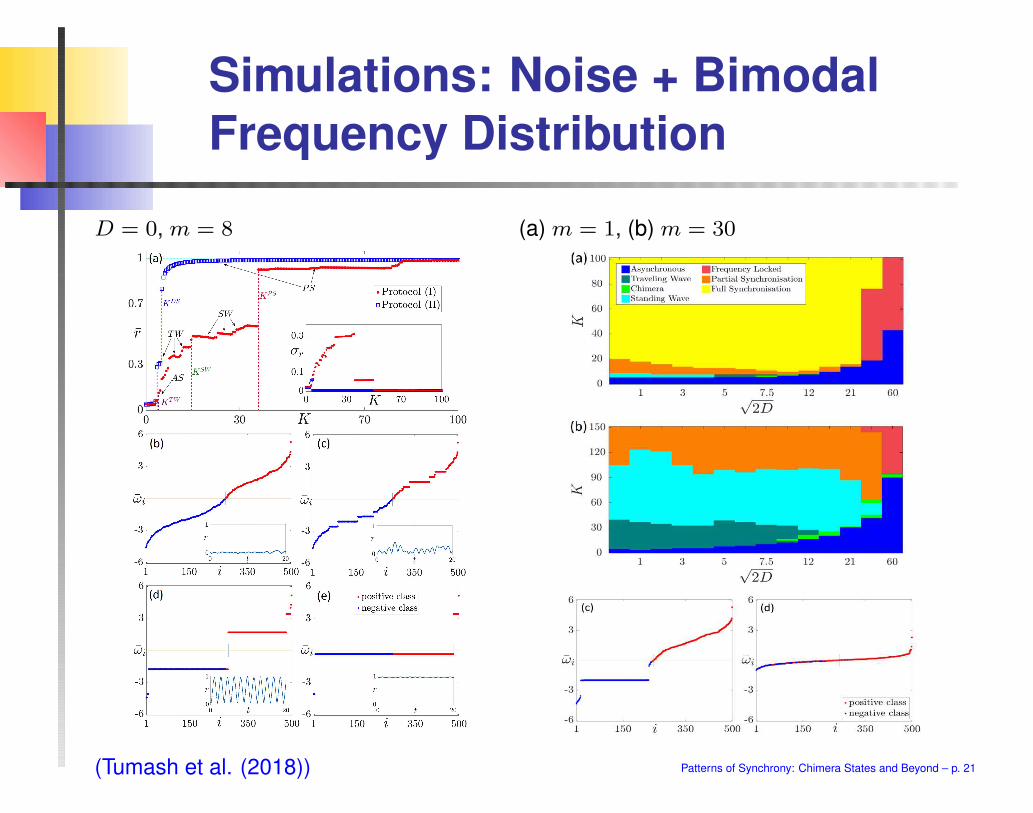
Simulations: Noise + Bimodal
Frequency Distribution
D = 0, m = 8 (a) m = 1, (b) m = 30
(Tumash et al. (2018)) Patterns of Synchrony: Chimera States and Beyond – p. 21

Bestiary
Patterns of Synchrony: Chimera States and Beyond – p. 22

Further works: diluted network
+ g(Ω) unimodal
Constraint 1 : the random matrix is symmetric
Constraint 2 : the in-degree is constant and equal to Nc
0 1 2 3 4 5 6
K
0
0.2
0.4
0.6
0.8
1
r
Nc=N
Nc=5
Nc=10
Nc=15
Nc=25
Nc=50
Nc=125
Nc=250
Nc=500
Nc=1000
(a)
0.01 0.1 1
Nc/N
0
0.5
1
1.5
2
2.5
3
Wh
N=500N=1000N=2000
0 3 6 9
K0
0.2
0.4
0.6
0.8
1
r
Wh
Diluted or fully coupled systems (whenever the coupling is properly rescaled with
the in-degree) display the same phase-diagram
For very small connectivities the transition from hysteretic becomes continuous
By increasing the system size the transition will stay hysteretic for extremely small
percentages of connected (incoming) linksPatterns of Synchrony: Chimera States and Beyond – p. 23

Further works: g(Ω) bimodal
0 10 20 30
K
0
0,2
0,4
0,6
0,8
1
r
KPSK
SW
KTW
PS
SW
TW
Globally coupled network
Traveling Wave (TW): a single
cluster of oscillators, drifting
together with a velocity Ω0
Standing Wave (SW): two
clusters of drifting oscillators with
symmetric opposite velocities
±Ω0
Partially Synchronized state (PS):
a cluster of locked rotators with
zero average velocity
(Olmi, Torcini (2016))
Patterns of Synchrony: Chimera States and Beyond – p. 24

Further works: diluted network
+ g(Ω) bimodal
p = 0.25
m = 6
For bigger masses, larger values
of critical coupling are required to
reach synchronization
Nc = pN
The hysteretic loop decreases as
the network topology becomes
more sparse
(Tumash et al. (2018))
Patterns of Synchrony: Chimera States and Beyond – p. 25
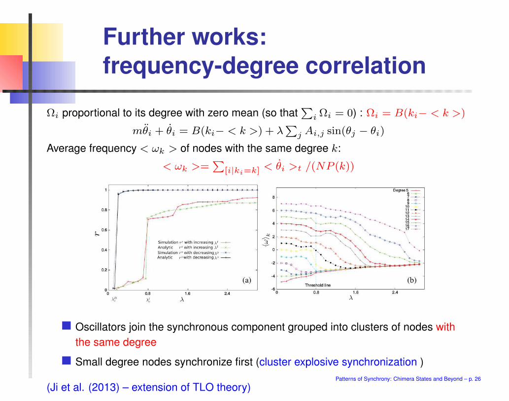
Further works:
frequency-degree correlation
Ωi proportional to its degree with zero mean (so that∑
i Ωi = 0) : Ωi = B(ki− < k >)
mθi + θi = B(ki− < k >) + λ∑
j Ai,j sin(θj − θi)
Average frequency < ωk > of nodes with the same degree k:
< ωk >=∑
[i|ki=k] < θi >t /(NP (k))
Oscillators join the synchronous component grouped into clusters of nodes with
the same degree
Small degree nodes synchronize first (cluster explosive synchronization )
(Ji et al. (2013) – extension of TLO theory)Patterns of Synchrony: Chimera States and Beyond – p. 26

Further works: chimera state
Two symmetrically coupled populations of N oscillators with inertia
mθ(σ)i + θ
(σ)i = Ω+
2∑
σ′=1
Kσσ′
Nsin(θ
(σ′)j − θ
(σ)i − γ)
σ = 1, 2 identifies the population
θ(σ)i is the phase of the ith oscillator
in population σ
Ω is the natural frequency
γ = π− 0.02 is the fixed frequency lag
Kσ,σ > Kσ,σ′
The collective evolution of each population is characterized in terms of the macroscopic
fields ρ(σ)(t) = R(σ)(t) exp [iΨ(t)] = N−1∑N
j=1 exp [iθ(σ)j (t)].
In analogy with Abrams, Mirollo, Strogatz and Wiley, PRL (2008).
Patterns of Synchrony: Chimera States and Beyond – p. 27
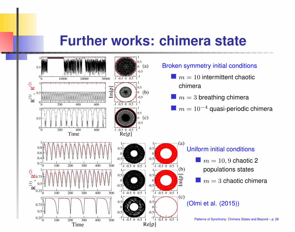
Further works: chimera state
Broken symmetry initial conditions
m = 10 intermittent chaotic
chimera
m = 3 breathing chimera
m = 10−4 quasi-periodic chimera
Uniform initial conditions
m = 10, 9 chaotic 2
populations states
m = 3 chaotic chimera
(Olmi et al. (2015))
Patterns of Synchrony: Chimera States and Beyond – p. 28

Further works: imperfect
chimera state
A ring of N non-locally coupled Kuramoto oscillators with inertia, each one connected to
its P nearest neighbours to the left and to the right with equal strength
mθi + ǫθi =k
2P+1
∑i+Pj=i−P sin(θj − θi − α)
The system is multistable
Imperfect chimera state: a
certain number of oscillators
split from synchronized do-
main
(Jaros et al. (2015))
Patterns of Synchrony: Chimera States and Beyond – p. 29
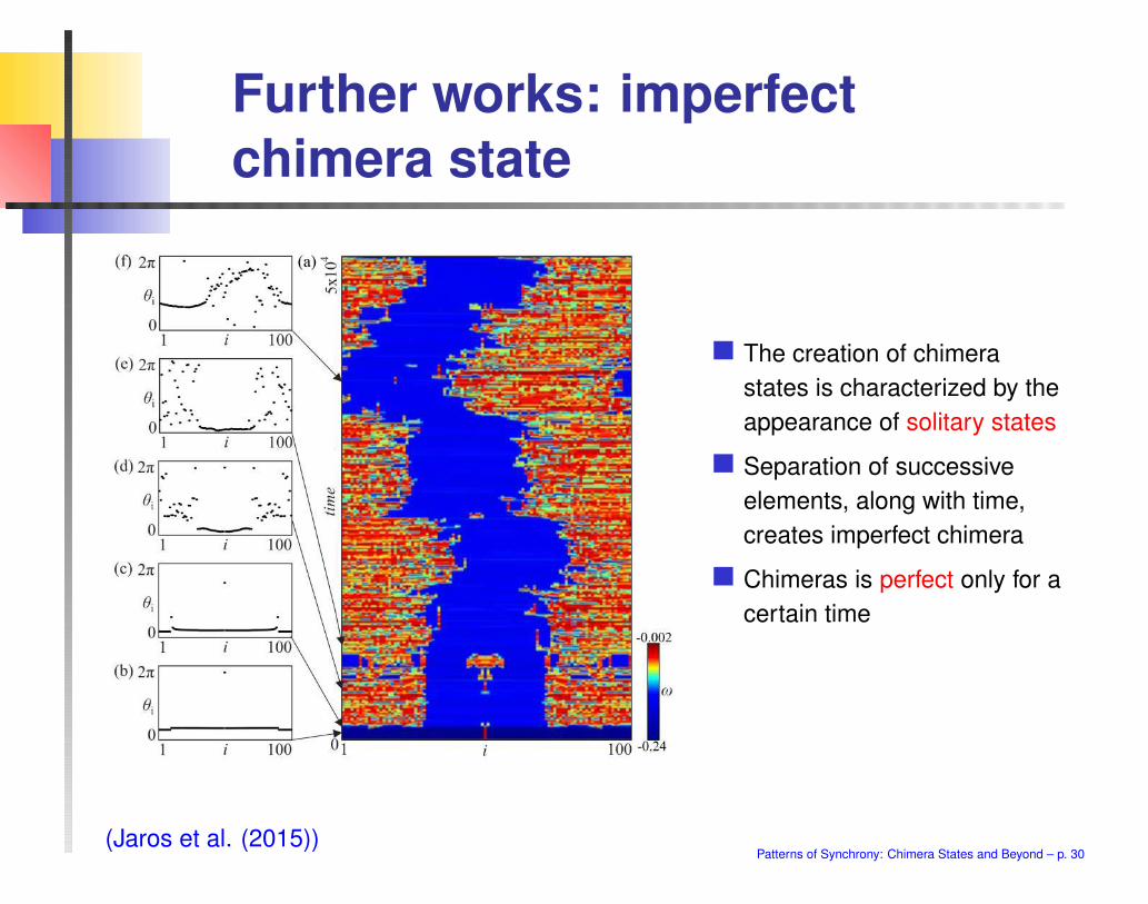
Further works: imperfect
chimera state
The creation of chimera
states is characterized by the
appearance of solitary states
Separation of successive
elements, along with time,
creates imperfect chimera
Chimeras is perfect only for a
certain time
(Jaros et al. (2015))Patterns of Synchrony: Chimera States and Beyond – p. 30
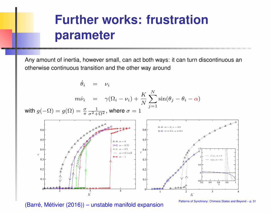
Further works: frustration
parameter
Any amount of inertia, however small, can act both ways: it can turn discontinuous an
otherwise continuous transition and the other way around
θi = νi
mνi = γ(Ωi − νi) +K
N
N∑
j=1
sin(θj − θi − α)
with g(−Ω) = g(Ω) = σπ
1σ2+Ω2
, where σ = 1
(Barré, Métivier (2016)) – unstable manifold expansionPatterns of Synchrony: Chimera States and Beyond – p. 31
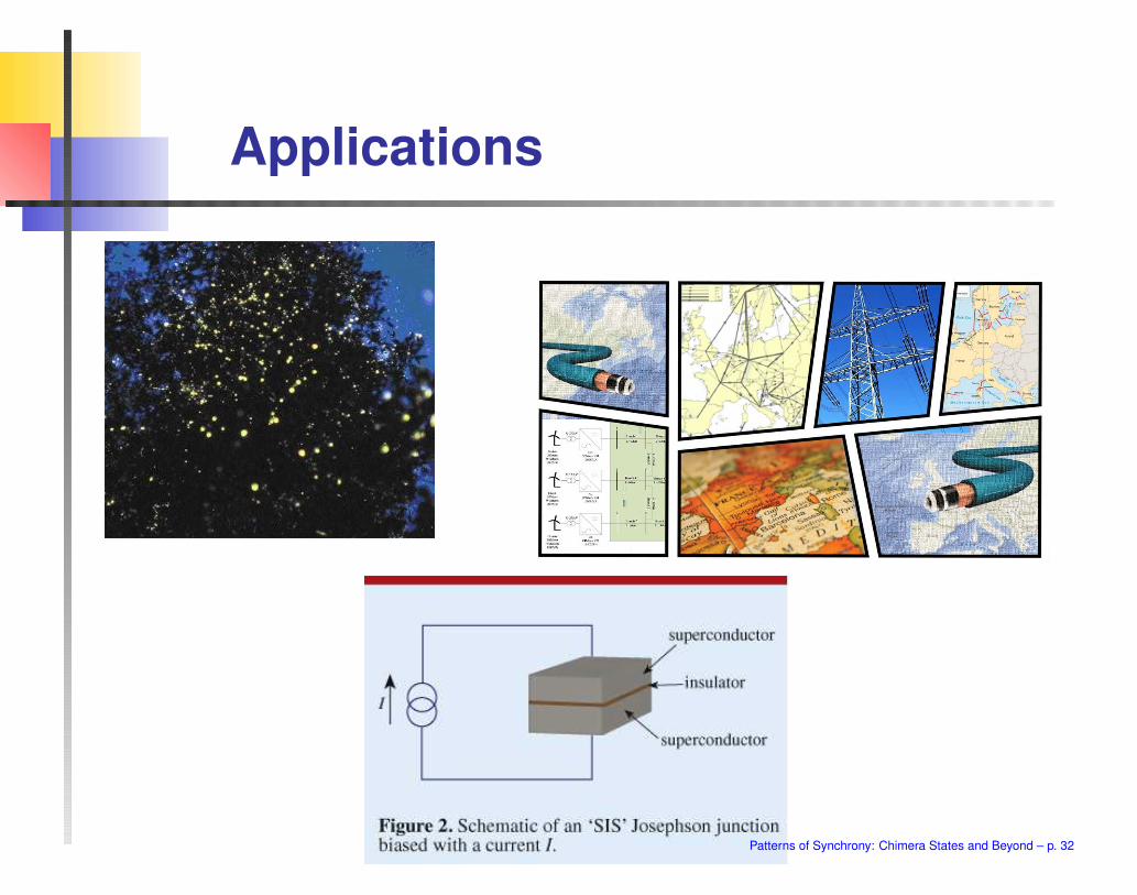
Applications
Patterns of Synchrony: Chimera States and Beyond – p. 32

Power Plants
A power plant consist of a boiler producing a constant power, as well as a turbine
(generator) with high inertia and some damping.
Transmitted power through a line: Pmax12 sin(θ2 − θ1).
Power plant + transmission line =power source that feeds energy into the system.
This energy can be accumulated as rotational energy or dissipated due to friction.
The remaining part is available for a user (the machine M ), provided that there
exists a phase angle difference ∆θ = θ2 − θ1 between the two mechanical
rotators (phase shift is necessary for ac power transmission)
Patterns of Synchrony: Chimera States and Beyond – p. 33
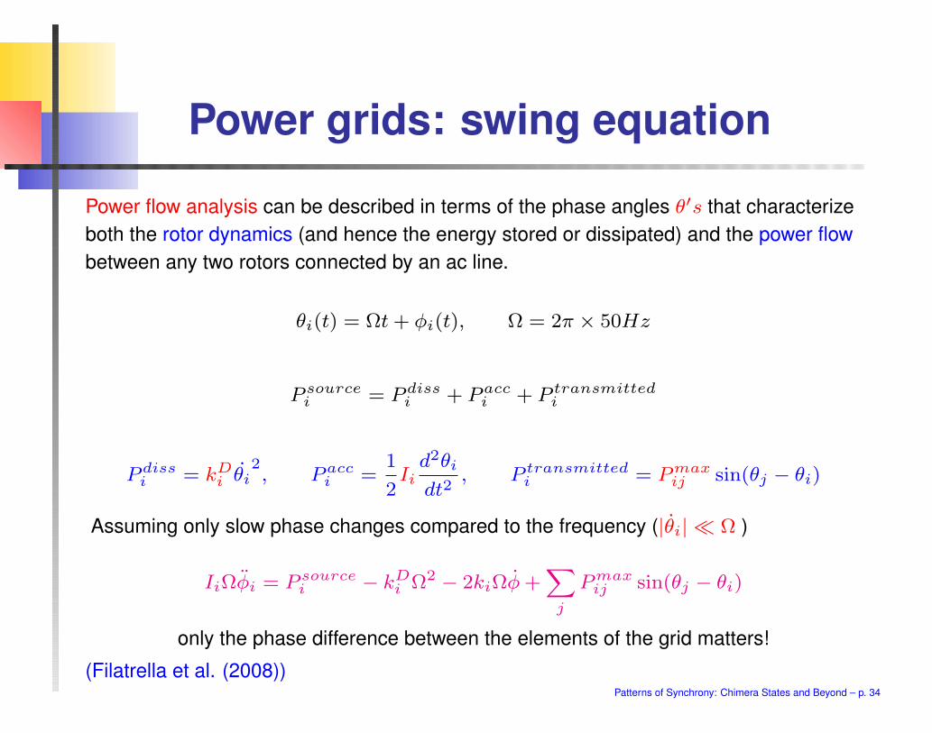
Power grids: swing equation
Power flow analysis can be described in terms of the phase angles θ′s that characterize
both the rotor dynamics (and hence the energy stored or dissipated) and the power flow
between any two rotors connected by an ac line.
θi(t) = Ωt+ φi(t), Ω = 2π × 50Hz
P sourcei = P diss
i + Pacci + P transmitted
i
P dissi = kDi θi
2, Pacc
i =1
2Ii
d2θi
dt2, P transmitted
i = Pmaxij sin(θj − θi)
Assuming only slow phase changes compared to the frequency (|θi| ≪ Ω )
IiΩφi = P sourcei − kDi Ω2 − 2kiΩφ+
∑
j
Pmaxij sin(θj − θi)
only the phase difference between the elements of the grid matters!
(Filatrella et al. (2008))Patterns of Synchrony: Chimera States and Beyond – p. 34

Power grids: parameters
Every element i is described by the same rescaled equation of motion with a parameter
Pi giving the generated (Pi > 0) or consumed (Pi < 0) power
d2φi
dt2= Pi − αi
dφ
dt+
∑
j
Kij sin(θj − θi)
where Kij =Pmaxij
IiΩ, Pi =
Psourcei −kD
i Ω2
IiΩ, αi =
2ki
Ii,∑
j Pj = 0.
Large centralized power plants generating P sourcei = 100Mw each
Each synchronous generator has a moment of inertia of Ii = 104kgm2
The mechanically dissipated power kDi Ω2 usually is a small fraction of P source
Additional sources of dissipation are not taken into account
A transmission capacity for major overhead power line is up to Pmaxij = 700MW
The transmission capacity for a line connecting a small city is Kij ≤ 102s2
αi = 0.1s−1, Pi = 10s−2 for large power plants, Pi = −1s−2 for a small city
Patterns of Synchrony: Chimera States and Beyond – p. 35
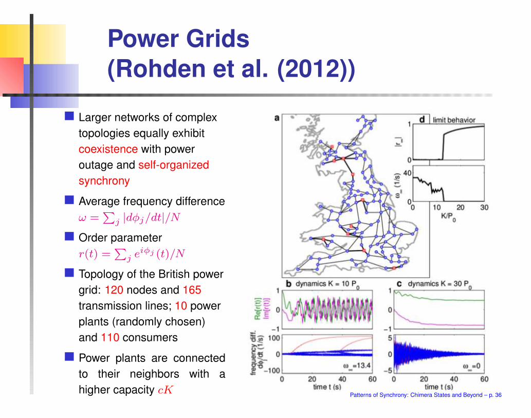
Power Grids
(Rohden et al. (2012))
Larger networks of complex
topologies equally exhibit
coexistence with power
outage and self-organized
synchrony
Average frequency difference
ω =∑
j |dφj/dt|/NOrder parameter
r(t) =∑
j eiφj (t)/N
Topology of the British power
grid: 120 nodes and 165
transmission lines; 10 power
plants (randomly chosen)
and 110 consumers
Power plants are connected
to their neighbors with a
higher capacity cKPatterns of Synchrony: Chimera States and Beyond – p. 36

Power Grids Stability
(Rohden et al. (2012))
How does decentralization impact the system’s stability to dynamic perturbations?
Replace large power plants (Pj = 11P0) by smaller ones (Pj = 1.1P0).
Test the stability against fluctuations by transiently increasing the power demand of
each consumer during a short time interval ( the condition∑
j Pj = 0 is violated)
After the perturbation is switched off, the system either relaxes back to a steady
state or does not, depending on the strength of the perturbation
The maximally allowed perturbation strength shrinks with decentralization, but still
all grids are stable up to strengths a few times larger than the unperturbed load
Patterns of Synchrony: Chimera States and Beyond – p. 37
Josephson Junctions
The Josephson effect is the phenomenon of supercurrent, a current that flows
indefinitely long without any voltage applied, through a Josephson junction (JJ)
A JJ consists of two or more superconductors coupled by a weak link, which can
consist of a thin insulating barrier, a short section of non-superconducting metal, or
a physical constriction that weakens the superconductivity at the point of contact
The Josephson effect is an example of a macroscopic quantum phenomenon,
predicted by Brian David Josephson in 1962 (Josephson (1962))
The DC Josephson effect had been seen in experiments prior to 1962, but had
been attributed to “super-shorts” or breaches in the insulating barrier
The first paper to claim the discovery of Josephson’s effect, and to make the
requisite experimental checks, was that of (Anderson and Rowell (1963))
Before JJ, it was only known that normal, non-superconducting electrons can flow
through an insulating barrier (quantum tunneling). Josephson first predicted the
tunneling of superconducting Cooper pairs (Nobel Prize in Physics 1973).
A locally coupled Kuramoto model with inertia can be derived from a coupled resistively
and capacitively shunted junction eqs for an underdamped ladder with periodic boundary
conditions (Trees et al. (2005)): good agreements are achieved for phase and frequency
synchronization
Patterns of Synchrony: Chimera States and Beyond – p. 38

ReferencesB. Ermentrout, Journal of Mathematical Biology 29 , 571 (1991)
EE. Hanson, Cellular Pacemakers, ed. D.O. Carpenter, Vol. 2 (Wiley, New York, 1982)
pp. 81-100
S. H. Strogatz, Nonlinear Dynamics And Chaos: With Applications To Physics, Biology,
Chemistry, And Engineering, 1st Edition, Westview Press (1994)
B. R. Trees, V. Saranathan, D. Stroud, Physical Review E 71 (1) (2005) 016215
G. Filatrella, A. H. Nielsen, N. F. Pedersen, The European Physical Journal B 61 (4),
485-491 (2008)
H. D. Chiang, BCU Methodologies, and Applications, John Wiley & Sons (2011)
M. Levi, F. C. Hoppensteadt, W. L. Miranker, Quarterly of Applied Mathematics 36.2,
167-198 (1978)
H. A. Tanaka, A. J. Lichtenberg, S. Oishi, Physical Review Letters 78 (11) (1997)
2104-2107 (1997)
S. Olmi, A. Navas, S. Boccaletti, A. Torcini, Physical Review E 90 (4), 042905 (2014)
S. Gupta, A. Campa, S. Ruffo, Physical Review E 89 (2) 022123 (2014)
J. A. Acebrón, L. L. Bonilla, R. Spigler, Physical Review E 62 (3) 3437-3454 (2000)
J. A. Acebrón, R. Spigler, Physical Review Letters 81 (11) 2229-2232 (2008)
Patterns of Synchrony: Chimera States and Beyond – p. 39

ReferencesH. Hong, M. Choi, B. Yoon, K. Park, K. Soh, Journal of Physics A: Mathematical and
General 32 (1) L9 (1999)
L. L. Bonilla, Physical Review E 62 (4), 4862-4868 (2000)
H. Hong, M. Y. Choi, Physical Review E 62 (5) (2000) 6462-6468
L. Tumash, S. Olmi, E. Schöll, EPL 123, 20001 (2018)
S. Olmi, A. Torcini, in Control of Self-Organizing Nonlinear Systems, 25-45 (2016)
P. Ji, T. K. D. Peron, P. J. Menck, F. A. Rodrigues, J. Kurths, Physical Review Letters 110
(21), 218701 (2013)
S. Olmi, E. A. Martens, S. Thutupalli, A. Torcini, Physical Review E 92 (3) 030901 (2015)
P. Jaros, Y. Maistrenko, T. Kapitaniak, Physical Review E 91 (2) 022907 (2015)
J. Barré, D. Métivier, Physical review letters 117.21, 214102 (2016)
M. Rohden, A. Sorge, M. Timme, D. Witthaut, Physical Review Letters 109 (6), 064101
(2012)
B. D. Josephson, Physics letters 1 (7): 251-253 (1962)
P. W. Anderson, J. M. Rowell, Physical Review Letters 10 (6): 230 (1963)
Patterns of Synchrony: Chimera States and Beyond – p. 40

Extension of the Mean Field
Theory
In principle one could fix the discriminating frequency to some arbitrary value Ω0 and
solve self-consistently
r = rL + rD
rI,IIL = Kr
∫ θ0
−θ0
cos2 θg(Kr sin θ)dθ rI,IID ≃ −mKr
∫ ∞
−Ω0
1
(mΩ)3g(Ω)dΩ
This amounts to obtain a solution r0 = r0(K,Ω0) by solving
∫ θ0
−θ0
cos2 θg(Kr0 sin θ)dθ −m
∫ ∞
−Ω0
1
(mΩ)3g(Ω)dΩ =
1
K
with θ0 = sin−1(Ω0/Kr0). The solution exists if Ω0 < ΩD = Kr0.
⇒ A portion of the (K, r) plane delimited by the curve rII(K) is filled with the curves
r0(K) obtained for different Ω0 values.
Patterns of Synchrony: Chimera States and Beyond – p. 41

Drifting Clusters
(Olmi et al. (2014))
The amplitude of the oscillations of r(t) and the number of oscillators in the drifting
clusters NDC correlates in a linear manner
The oscillations in r(t) are induced by the presence of large secondary clusters
characterized by finite whirling velocities
At smaller masses oscillations are present, but reduced in amplitude. Oscillations
are due to finite size effects since no clusters of drifting oscillators are observed
Blue dashed line ⇒ estimated
mean field value rI by Tanaka et
al. (1997)
The mean field theory captures
the average increase of the order
parameter but it does not foresee
the oscillations
0 5 10 15 20
K
0
0.2
0.4
0.6
0.8
1
0 5 10 15 200
50
100
150
r min
,r m
ax
(rmax
-rmin
)*240
NDC
Patterns of Synchrony: Chimera States and Beyond – p. 42
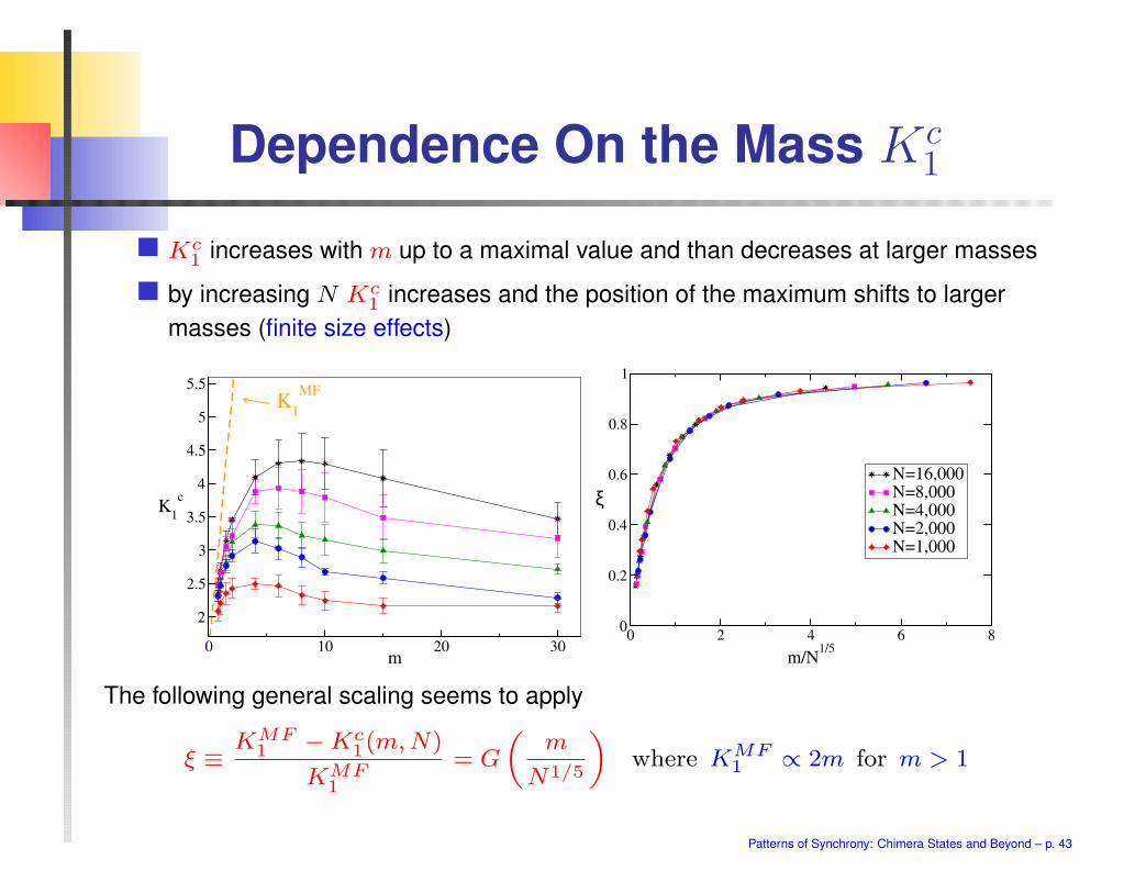
Dependence On the Mass Kc1
Kc1 increases with m up to a maximal value and than decreases at larger masses
by increasing N Kc1 increases and the position of the maximum shifts to larger
masses (finite size effects)
0 10 20 30m
2
2.5
3
3.5
4
4.5
5
5.5
K1
c
K1
MF
0 2 4 6 8
m/N1/5
0
0.2
0.4
0.6
0.8
1
ξN=16,000N=8,000N=4,000N=2,000N=1,000
The following general scaling seems to apply
ξ ≡ KMF1 −Kc
1(m,N)
KMF1
= G
(
m
N1/5
)
where KMF1 ∝ 2m for m > 1
Patterns of Synchrony: Chimera States and Beyond – p. 43

Dependence On the Mass Kc2
The TLO approach fails to reproduce the critical coupling for the transition from
asynchronous to synchronous state (i.e., Kc1), however it gives a good estimate of the
return curve obtained with protocol II from the synchronized to the aynchronous regime
0 5 10 15 20 25 30m
1.6
1.8
2
2.2
K2
c
K2
TLO
Kc2 initially decreases with m then saturates, limited variations with the size N
KTLO2 is the minimal coupling associated to a partially synchronized state given
by TLO approach for protocol II
KTLO2 exhibits the same behaviour as Kc
2 , however it slightly understimates the
asymptotic value (see the scale) Patterns of Synchrony: Chimera States and Beyond – p. 44
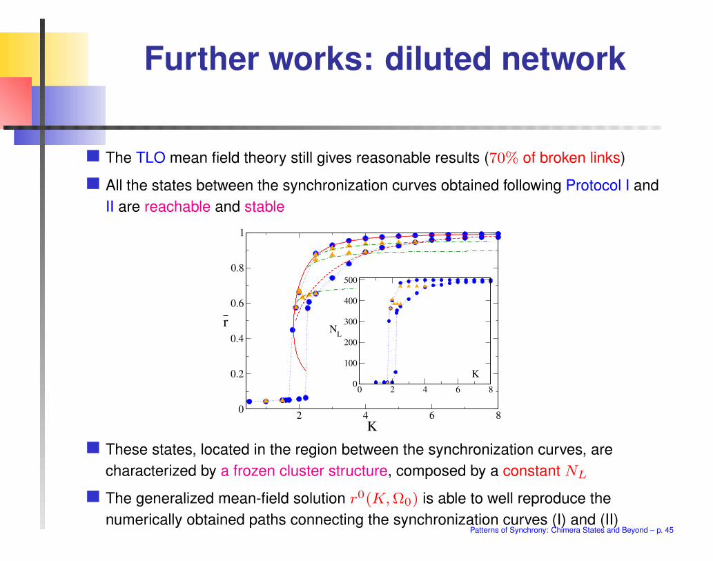
Further works: diluted network
The TLO mean field theory still gives reasonable results (70% of broken links)
All the states between the synchronization curves obtained following Protocol I and
II are reachable and stable
2 4 6 8
K
0
0.2
0.4
0.6
0.8
1
r
0 2 4 6 8
K0
100
200
300
400
500
NL
These states, located in the region between the synchronization curves, are
characterized by a frozen cluster structure, composed by a constant NL
The generalized mean-field solution r0(K,Ω0) is able to well reproduce the
numerically obtained paths connecting the synchronization curves (I) and (II)Patterns of Synchrony: Chimera States and Beyond – p. 45
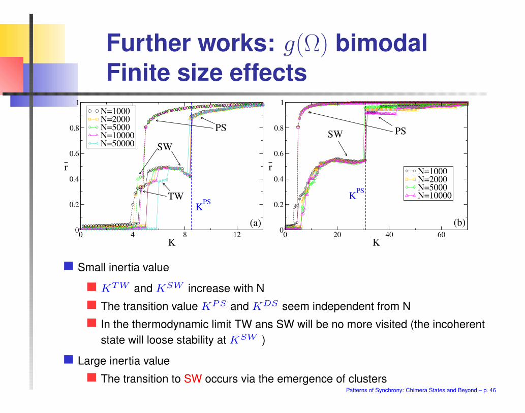
Further works: g(Ω) bimodal
Finite size effects
0 4 8 12
K
0
0.2
0.4
0.6
0.8
1
r
N=1000N=2000N=5000N=10000N=50000
(a)
TW
SW
PS
KPS
0 20 40 60
K
0
0.2
0.4
0.6
0.8
1
r N=1000N=2000N=5000N=10000
(b)
KPS
SW PS
Small inertia value
KTW and KSW increase with N
The transition value KPS and KDS seem independent from N
In the thermodynamic limit TW ans SW will be no more visited (the incoherent
state will loose stability at KSW )
Large inertia value
The transition to SW occurs via the emergence of clustersPatterns of Synchrony: Chimera States and Beyond – p. 46

Italian High Voltage Power GridEach node is described by the phase:
φi(t) = ωAC t+ θi(t)
where ωAC = 2π 50 Hz is the standard
AC frequency and θi is the phase devi-
ation from ωAC .
Consumers and generators can be
distinguished by the sign of parameter
Pi:
Pi > 0 (Pi < 0)
corresponds to generated (consumed)
power.
θi = α
−θi + Pi +K∑
ij
Ci,j sin(θj − θi)
Average connectivity < Nc >= 2.865
[ Filatrella et al., The European Physical Journal B (2008)]Patterns of Synchrony: Chimera States and Beyond – p. 47
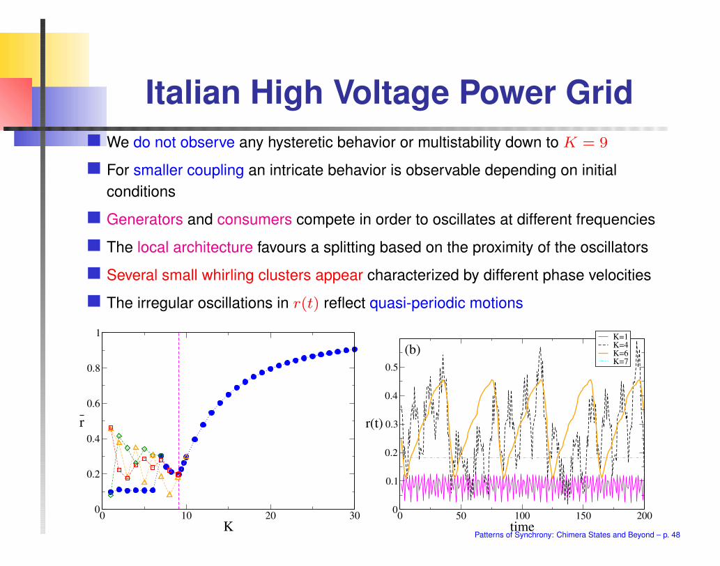
Italian High Voltage Power Grid
We do not observe any hysteretic behavior or multistability down to K = 9
For smaller coupling an intricate behavior is observable depending on initial
conditions
Generators and consumers compete in order to oscillates at different frequencies
The local architecture favours a splitting based on the proximity of the oscillators
Several small whirling clusters appear characterized by different phase velocities
The irregular oscillations in r(t) reflect quasi-periodic motions
0 10 20 30
K
0
0.2
0.4
0.6
0.8
1
r
0 50 100 150 200
time
0
0.1
0.2
0.3
0.4
0.5
r(t)
K=1K=4K=6K=7
(b)
Patterns of Synchrony: Chimera States and Beyond – p. 48

Italian High Voltage Power Grid
By following Protocol II
the system stays in one cluster up to K = 7
at K = 6 wide oscillations emerge in r(t) due to the locked clusters that have
been splitted in two (is this also the origin for the emergent multistability?)
By lowering further K several whirling small clusters appear and r becomes
irregular
Patterns of Synchrony: Chimera States and Beyond – p. 49