the impact of proximity to urban center on … nuru... · seid nuru and holger seebens: the impact...

105

THE IMPACT OF PROXIMITY TO URBAN CENTER ON CROP PRODUCTION CHOICE AND RURAL

INCOME: EVIDENCES FROM VILLAGES IN WOLLO, ETHIOPIA

Seid Nuru Ali1 and Holger Seebens2

Abstract This article attempts to demonstrate how proximity to urban centers influences households' decision to allot their agricultural land to the production of either staple crops or high value cash crops. By applying fractional logit estimation technique on data collected from villages in Wollo of the Amhara Regional State in 2006, it has been found that proximity to urban centers, access to road, and education of the head of the household determine the crop choice in favor of the production of high value cash crops. While the purely liquid wealth positively affects the allocation of land for the production of cash crops, the direction of the impact of livestock on crop choice is found to depend on the particular location of the activities in relation to urban (market) centers. The pattern of crop choice has been translated into a variation in the level of per capita income across villages. Households operating in those villages located far from urban centers with no access to road are found to be the poorest among the villages covered by the study. Key Words: Location, Crop Choice, Rural Income, Fractional Logit

JEL Classification: D13, Q12, Q15

1 Senior fellow at the Ethiopian Economic Policy Research Institute, Ethiopian Economics Association, Addis Ababa 2 Assistant professor at Department for Agricultural Economics and Rural Development, University of Göttingen Acknowledgment: We are grateful to Prof. Stephen Klasen and the anonymous referees.

Seid Nuru and Holger Seebens: The impact of proximity to urban center on crop…

106

1. Introduction Early thinking on the relation between location and crop choice dates back to the 19th century owing to von Thünen who first formally theorized the importance of location in shaping the duality between the rural and urban economy. In his ‘Isolated State’, Thünen portrays an economy that consists of an urban center surrounded by homogenous agricultural land which differs only in terms of distance from the urban center. Agricultural produces from the land around a town are transported to the town for trading. Crop choices depend on the cost effectiveness of each crop in terms of transportation. According to Thünen’s portrayal, in the inner ring around the town, crops which are costly to transport (such as vegetables) are produced. At the outer annulus of the rings, crops involving lower transport costs (such as grain) are grown (Samuelson, 1983; Fujita and Thisse, 2002).

Looking beyond Thünen’s model, observations show that the decision of households located in the outer annulus to produce grains may not be entirely driven by price incentives but could also be an outcome of their desire to be self-sufficient in staple crops in order to smooth consumption. Assuming other factors being constant, high value cash crops can be costly to bring to the market if they are grown in locations far from urban centers. Inherent to different distances of villages from the urban centers is, thus, an unequal distribution of income.

Recent literature on crop choice focuses on uncertainties arising from weather conditions and price shocks. It has been widely argued that various forms of uncertainties contribute to the subsistent nature of many rural areas in developing countries (Dillon and Scandizzo, 1978; Fafchamps, 1992; Dercon, 1996; Ayalew, 2003). In response to this, rural households have developed different strategies to cope with the risk associated with agricultural production. Diversification has been conceived as a feasible insurance strategy, although often implies lower returns. Price fluctuations can be compensated if households cultivate a wide portfolio of crops, among which staple crops—tending to be more stable in terms of prices—constitute an important safety measure. In particular, poor and risk-averse households tend to ensure self-sufficiency in staple crops leading to the limitation of diversification to only different kinds of staple crops. The impact of risk on crop choice may vary across locations. Even in periods of stable and high prices for cash crops, households’ decision to engage in the production of cash crops depends on transportation costs, which in turn depend

Ethiopian Journal of Economics, Volume XX No. 2, October 2011

107

on the distance of the particular plot or village from the market. For instance, markets for logs and lumber of eucalyptus are well established in urban centers of Ethiopia. However, households living far from urban centers do not grow eucalyptus trees in significant magnitude even on their marginal land because eucalyptus growers living closer to urban centers outbid in the market. One reason for this is higher transportation cost. Distance to markets has thus an important influence on the development prospects of remote villages. Decisions by households to allocate the bulk of land to the production of less valued staple crops results in low surplus and low incomes, implying that the incidence of poverty is likely to increase with distance away from urban centers. This article attempts to look into how the location of an agricultural activity in relation to markets in urban centers affects the production of high value cash crops using cross sectional data collected from six villages in Wollo, Ethiopia. It also shows the associated disparity in income by location. The remaining part of the paper is organized as follows. Section 2 highlights descriptive facts from surveyed villages. Section 3 presents a simple theoretical framework. Section 4 deals with the econometric analysis. Section 5 concludes.

2. Crop Choice in Selected Villages of Ethiopia by Location According to the 2007 population census, Ethiopia’s population is estimated to be about 88 million people in 2011. The population is growing at a rate of 2.8 percent annually. About 84 percent of the population makes a living from subsistent agriculture accounting for 43 percent of GDP (MoFED, 2011). The country exhibits one of the lowest rates of urbanization where only 16 percent dwells in urban centers. As a result, size of arable land per household decreases making the land issue critical in transforming the Ethiopian economy. Average land size in the country hovers around 0.97 to 1.2 hectare per household. This is equivalent to a mere 0.2 hectare per head (CSA, 2010, 2011).

Ethiopian farmers mainly focus on the production of staple crops except for coffee for which an already established international market exists. One of the major factors for this is believed to be a poorly developed transport network and low demand from the urban center. According to the national data from Central Statistical Agency (CSA), in 2005, 84.3 percent of rural households in Ethiopia, excluding nomadic areas, live on crop and livestock production. In 2011, about 87 percent of the total production of major crops is accounted by cereals. If we


108

exclude teff3 which is both staple and cash crop, the share of the mainly staple crops in the major crop production is as high as 70 percent. Pulses which are predominantly cash crops have a share of 9.5 percent (CSA, 2005, 2011).

2.1 Location

The study covers six villages in four locations in Wollo, eastern part of the Amhara Regional State. The survey was conducted in the year 2006. The villages were systematically selected based on their increasing distance from major and district towns. The survey also accounts for agro-ecological differences. About 252 households were randomly selected from the villages. The distance between the reference district town and the nearest villages to the town is about 4 kilometers. The farthest village is 20 kilometers away from the nearest district town. Proximity to major towns is also considered. The major towns that are taken as references are Dessie and Woldiya. Dessie is the capital of South Wollo Zone (one of the eleven administrative Zones in the Region) and has an estimated population of 169,000. Woldiya is the capital of North Wollo Zone with an estimated population of 43,000. The two towns are 120 kilometers apart along the main Addis Ababa – Mekele road. District towns include Kutaber and Mersa.

One of the villages covered by the study called Alasha is located in Kutaber district some 12 kilometers from Dessie. The nearest district town to Alasha is Kutaber with an estimated population of 5,000. Two major attributes of the village compared to other survey areas in terms of location are (i) it is the nearest village to major urban centers, and (ii) it is located in the highland plateau characterized by a relatively cool climate.

The other study site, Mersa Zuria area, includes three villages intercepting the district town Mersa on either side of the Dessie-Woldiya road. Mersa has an estimated population of 6,500. The villages have easy access to the market primarily due to their proximity to the major Addis Ababa-Mekele road via Mersa and Woldiya. Besides, the villages are nearer to the district town, Mersa, and the Zone town Woldiya. Among the three villages, Buhoro has significant access to irrigation partly due to availability of tributary rivers.

The third study site is Girana. It is located about 7 kilometers east of the Addis Ababa-Mekele road. There is a gravel road linking the village to the major

3 Teff is an indigenous grass growing in Ethiopia which is used to make Ethiopian staple bread called ‘injera’.


109

highway. The major attribute of the village is that it has some tributaries which allow for irrigating a significant part of land. Moreover, there is weekly open market in the village attracting people from the surrounding villages.

Among the villages covered by the study, Habru-Ligo has the farthest distance from both urban centers and major roads, and even lacks feeder road. Individuals have to travel a minimum of three hours back and forth on foot on difficult terrains to work on their land. About 25 to 30 percent of the land possessed by the villagers is irrigable.

2.2 Land size and crop choice

The average land size per household ranges from 0.61 hectare in Alasha area to about 1 hectare in Mersa Zuria area. Although Alasha and Kullie have similar distance from district towns, per capita land size in Alasha is lower than in Kullie and even less than that of Menentela which is closest to the next district town. The pattern is similar in term of per capita land size where Alasha has the lowest with 0.13 hectare and Mersa Zuria has the highest with 0.27 hectare. Girana and Habru-Ligo have a roughly equal size of per capita land holding which is about 0.14 hectare.

Table 1: Location and Land Size by Village, 2006

Distance from

District Town

(in km)

Distance from Major Towns (in km)

Land Size per

Household (in hectare)

Proportion of Land Allotted

for Purely Cash Crop and Eucalyptus (%)

Dessie Woldiya

Alasha 7 12 geographically

remote 0.613 7.9

Mersa Zuria 1.020 18.2 Menentela 4 94 20 0.822 12.2 Kullie 7 97 25 1.000 9.4 Buhoro 8 98 20 1.160 28.3

Girana 15 75 50 0.666 19.9 Habru-Ligo 20 85 60 0.643 0.9

In terms of land allocation, Buhoro exhibits the highest share of land allotted for the production of cash crops (about 28 percent) while Habru-Ligo has the lowest share which is less than 1 percent. Major cash crops produced are sugarcane, fruits (orange, papaya, guava), coffee, and vegetables. The staple crops include sorghum of various varieties, and teff in villages other than Alasha. Teff is used


110

both as a cash crop and staple food due to its high value in urban markets as it is the major staple for the urban population. During periods of poor harvest, households usually sell their teff and buy other cheaper staple crops such as sorghum for household consumption. However, since teff has low productivity compared to sorghum and maize, households in the study areas allot only a small portion of their limited land for the production of this crop unlike other regions which are endowed with large land size and specialize in the production of the crop on a large scale. Households in Alasha area produce wheat, barley, oats, and pulses.

2.3 Patterns of income

Data on the level of income of households by source has been collected from the villages under study. Among those villages, Mersa Zuria area is relatively affluent with a per capita income of 1830 Birr. This is well above the average per capita national income of about 1300 Birr recorded in 2005 (NBE, Annual Report 2006). Buhoro with a relatively better access to irrigation is specialized in cash crop production. Unlike other villages, 47.5 percent of its income comes from cash crops. The peasants’ involvement in the production of high value cash crops in the area is reflected by the fact that about 48 percent of their income comes from 28 percent of their land. Kullie and Menentela, where irrigable land is lacking, the highest share of their income is derived from commercial livestock farming. About 24 percent of household income in Menentela area and 26 percent of the income in Kullie come from livestock farming.

Habru-Ligo has the lowest per capita income (about 520 Birr) among the villages covered by the survey. A typical rural farmer in Habru-Ligo earns just 23 percent of what a typical farmer in Buhoro earns. Though the village has irrigable land, cash crop production is not very common. Peasants in the area do not invest in commercial livestock even though the village is well endowed with suitable conditions for animal husbandry. Households raise cattle, goats and sheep mainly as a buffer stock.


111

Table 2: Sources of Income of Households by Village, 2006

Per

cap

ita in

com

e (i

n B

irr)

Source of Household Income and their Contribution to Total Income (%)

SSta

ple

crop

s

CC

ash

crop

s

EE

ucal

yptu

s

WW

age

Rem

ittan

ce

from

Abr

oad

Rem

ittan

ce

from

Tow

ns

Rur

al

Ent

erpr

ise

SSal

e of

A

nim

al

Alasha 934 53.7 2.9 18.3 1.6 2.1 1.6 3.1 12.8

Mersa Zuria 1830 31.2 23.7 9.6 5.3 7.6 2.6 0.0 16.8

Menentela 1545 35.3 0.8 10.4 6.7 15.1 5.0 0.0 24.0

Kullie 1079 47.5 0.6 3.7 8.4 8.3 0.0 0.0 25.5

Buhoro 2298 22.5 47.5 11.2 3.1 2.3 2.0 0.0 8.7

Girana 1087 45.6 20.3 0.1 6.3 14.8 0.6 2.4 3.7

Habru-Ligo 520 86.3 3.8 0.1 1.8 2.2 0.0 0.7 3.2

Source: Own computations from the survey data

Besides crop production, villagers operating nearer to urban centers allot more plots of land for fast growing trees in particular eucalyptus than those located far from urban centers. This partly depends on the type of slope and soil fertility of the plot of land possessed by peasants. In Alasha, hilly and marginal land which is held by peasants privately is largely covered by eucalyptus forests which have demand from urban centers for purposes of construction and energy supply. About 18 percent of household income in Alasha comes from the sale of logs of eucalyptus. In Menentela and Buhoro, between 10 and 11 percent of household income is derived from selling eucalyptus.

3. Theoretical Framework on Location, Crop choice and Rural Income

3.1. Background

We model a Thünen type of environment where rural households make a living from income that is generated from their farming activities. Households dwell and operate at different distance from urban centers. Each household consists of working household members who maximize a joint utility function. Labor time is optimally allocated between agricultural activities and off-farm income generating activities, most importantly employment in the urban centers. However, to make the analysis tractable, the household is assumed to consist of a single individual only.


112

Agricultural activities involve mainly crop production and animal husbandry. Crop production, which is the mainstay of rural households, involves various items of products, of which the production technologies may differ. We restrict our attention to two major activities, namely, production of stable crops and production of cash crops. In fact, about 74 percent of the income of households in the villages covered by the survey comes from crop cultivation.

The household produces crops by combining land and other inputs such as labor, animal draft power, fertilizer and pesticides. Part of the staple crop and a significant share of the cash crop have to be sold to purchase manufactured goods for consumption. A household not producing sufficient staple crops thus falling short of home consumption has to purchase additional food from the market using the proceeds from the sale of cash crops.

The decision to produce a particular item depends on the relative distance of the activity from the town. Moreover, unlike the Thünen’s rings, the land surrounding the town needs not to be uniform so that villages at the same distance from town specialize in different crops. In what follows, we attempt to analyze how location affects the decision of a household to allot a plot of land for either staple or purely cash crops.

3.2 Production technologies and costs

Land is a limited resource. As a result, households rationally decide to invest in high value crops that maximize income per unit of land. Cash crops are preferred not necessarily because they give high yields per unit of land but because they fetch high market value, most importantly in urban centers. Some cash crops such as coffee are not consumed for their nutritional values. Other crops such as vegetables are highly perishable. Staple crops on the other hand give more security to the household against low prices because the household can still use staple crops for own consumption.

The production of the two crops requires factors such as land and labor. We further assume that labor is not a binding constraint for agricultural production. The household is assumed to have a single unit of labor and a single plot of land that can be allotted to the production of cash crops and staple crops. Let lc and ls represent the shares of land for cash and staple crops, respectively, so that lc

+ ls = 1. Using lc portion of land, the household produces qc units of cash crops to be sold at price pc in urban centers. The remaining land (ls = 1- lc) is used to produce


113

qs units of staple crop. Part of this crop will be consumed at home and any surplus is sold at the market at a price of ps. The production function of the two types of crops that relate the output per labor qi to a fraction of a unit of land li

is, therefore, given by: 4

( )c c cq A f l=

( )s s sq A g l= (1)

where qi denotes output per unit of labor and Ac and As are the levels of technology required to produce cash and staple crops, respectively. The production functions are assumed to fulfill the standard conditions:

( )' 0 , cf l > ( ) '' 0 ;cf l <

( )' 0 , sg l > ( )'' 0. sg l <

where '(.)f , '(.)g and ''(.)f , ''(.)g refer to the first and second order

derivates of the production function with respect to land respectively. The technology required to produce staple crops, As, is considered a numéraire to which the technology Ac can be compared. Thus, As is set to unity so that

( )s sq g l= .

It is assumed that the decision to produce cash crops also depends on the technical know-how about the production of the particular cash crop. An individual might be a quick innovator in terms of acquiring new technology if he

4 Practically, some cash crops such as coffee, orange, and pawpaw have maturity period of two to five years. There are also some crops such as vegetables and oilseeds with a maximum maturity period of one year. Ayalew (2003) noted this issue and has taken the opportunity cost of land in terms of yield of annual crops as a result of longer maturity period of coffee trees into account in his model. However, it is customary in the area under study that the land under permanent cash crops can at the same time be used for the production of annual crops until the cash crops grew to a full‐fledged tree. Thus, it is not harmful to continue the analysis without considering the opportunity cost of land due to long gestation period of permanent crops.


114

has some formal education. The technological parameter in the production function of the cash crop is given by:5

0 Ec cA A eψ= (2)

where Ac

0 is some indigenous knowledge of the technology, E is level of education

(say in years of schooling), and ψ is a parameter. Given prices of cash crop and staple crops, the total monetary value of these crops is given by:

( ) ( )0c E c c s sy A e p f l p g lψ= + (3)

The household incurs production costs for each crop. Costs of production of each crop are proportional to land allotted to the production of the crops. Let wc and ws represent factor prices per unit of land. The associated cost of production of cash and staple crops are given by wclc and wsls.

The household also incurs transportation costs for both crops. We further assume that direct cost of transportation is the same for each crop. However, the cost of transportation varies depending on the amount of crop the household wants to sell. Household sell small shares of the staple crop because most of it is produced for home consumption. We assume that all cash crops produced by the household are sold6 and let n denote the share of staple crop that is marketable. Then, the total transportation cost with k unit price of transportation is given by kqcr and knqsr, where r is the distance between the village and the urban center. The household also faces cost due to the perishable nature of each crop. We define an index that measures the degree of the perishable nature of each crop in connection to transporting the surplus to the market. Let r be the distance of the

plot from the market place and maxir denote the maximum distance of the ith crop

5 The adoption of the technology once it is available is assumed to evolve exponentially according to

0 c c gtA A e= where g is the rate of innovation and t is time required to acquire the technique. The

rate of growth of technology is assumed to be a function of education over time, .g Eψ= 6 This assumption is only to make the analysis simple. Practically, part of the cash crops produced by the household is consumed by the household even though it might be in small proportion compared to staple crops.


115

beyond which the crop cannot be sold at the market due to its perishable nature. Then, the index for the ith crop is given by:

*

max

ii

rrr

= (4)

where:

*

max

0 01

ii

if rr

if r r=⎧

= ⎨ ≥⎩ so that [ ]* 0,1ir ∈.

If the crop produced at distance r is perishable, then it loses a value of *ir

monetary units per unit of crop. If almost all cash crops produced and n fraction of the staple crop are intended to be sold at their respective prices, and if all staple crops are not perishable, then the associated total cost incurred can be summarized by:

( ) *c s c c c c c s sC q nq kr r p q w l w l= + + + + (5)

Given the revenue function in Equation (3) and the cost function in Equation (5),

the profit π of the household is, therefore, given by:

( )( ) ( )( )*0c E c c c c s s c c s s

t A e f l p kr r p g l p nkr w l w lψπ = − − + − − −

(6)

3.3 The problem of the household

The household maximizes profit according to:

( )( ) ( )( )*0max

c

c E c c c c s s c c s s

lA e f l p kr r p g l p nkr w l w lψπ = − − + − − −

(7)

Taking the first order derivatives with respect to proportion of land under cash crop, the first order condition is:


116

( )( ) ( )( )*0 ' ' 0c E c c c c s s c s

c

d A e f l p kr r p g l p nkr w wdl

ψπ= − − − − − + =

This can be rearranged to give:

( ) ( )( ) ( )( )*0 0' ' 'c c E c c E c c c c s s sp A e f l A e f l kr r p w g l p nkr wψ ψ⎡ ⎤ ⎡ ⎤= + + + − −⎣ ⎦ ⎣ ⎦

(8)

The left hand side of Equation (8) is the value marginal product of land in the production of cash crops. The first term of the right hand side of the equation in square brackets is the marginal cost of producing and selling cash crops. The term in the second square bracket denotes the opportunity cost of production of cash crops at the net margin. In general, this condition says that an optimum allocation of the available plot of land between cash and staple crops ensures that the marginal product of land in the production of cash crops equals the foregone value of the marginal product of staple crops net of marginal costs of production in the alternative use plus direct marginal costs. It can be shown that the second order derivative of the profit function with respect to plot of land allotted for the production of cash crops is negative.

( )( )( ) ( )( )

2*

2 0 '' '' 0c E c c c c s s

c

d A e f l p kr r p g l p nkrd l

ψπ= − − + − <

By the assumption of diminishing returns to scale, ( )'' cf l and ( )'' sg l are

negative. The household produces cash crop if his optimization condition ensures

that unit profits are greater than unit costs so that ( )*c c cp kr r p> + and sells

his staple crop ifsp nkr> . This implies that the second derivative is negative.

Thus, the sufficient condition for maximization of profit is met. Note that the

second order derivative becomes positive if r*c is unity, that is if r ≥ rcmax.

Nonetheless, at r*c = 1, the household has no incentive to produce any cash crop as it would intuitively mean that all cash crops that have to be transported will be spoiled before they reach the market.


117

3.4 Comparative static analysis

In this section we examine the impact of varying the distance of producers to the urban centers and the level of education on land allocation decision. The first order condition can be re-written in the form of an implicit function F(.):

( )( )( ) ( )( )

*

*0

; , , , , , , , ,

' ' 0

c c s c s

c E c c c c s s c s

F l r r E p p w w k n

A e f l p kr r p g l p nkr w wψ= − − − − − + =

(9)

By totally differentiating the implicit function, we have:

( )( ) ( )( ){ }( ) ( ){ }( ){ }

0

0

0

*'' ''

* '' ... 0

' 'c E c s

cc E c c c c s sdF A e f l p kr r p g l p nkr dl

c E c c c cA e f l p kr r p dE

k A e f l ng l drψ

ψ

ψψ

= − − + −

+

⎡ ⎤+ − − + =⎢ ⎥⎣ ⎦

⎡ ⎤−⎣ ⎦

Holding other exogenous variables constant, the change in lc in response to a change in distance from the market is given by:

( ) ( )0 ' 'c E c sc k A e f l ng ldldr J

ψ⎡ ⎤−⎣ ⎦=

where:

( )( ) ( )( ){ }*0 '' ''c E c c c c s sJ A e f l p kr r p g l p nkrψ= − − + − .

Basically, J is the second order derivative of the profit function with respect to lc

which is negative. In the numerator, ( )' cf l and ( )' sg l , are positive by

assumption. We assume that the marginal product under cash crop production

( )( )0 'c E cA e f lψ is greater than the n fraction of the marginal productivity of land


118

for the production of staple crop, ( )( )' sng l . This implies that the term in the

numerator is greater than zero. Hence, we have:

( ) ( )0 ' '0

c E c sc k A e f l ng ldldr J

ψ⎡ ⎤−⎣ ⎦= <

That is, a unit variation in location across plots in relation to markets in the direction away from such markets leads to a decline in the share of land under cash crop production. Similarly, the direction of the impact of the index for the perishable nature of a cash crop can be shown to be negative. The higher the index (i.e. the more perishable the crop is), the less proportional land to be allotted for the production of the particular cash crop.

( )0

*

'0

c c E cc p A e f ldldr J

ψ

= < .

The direction of the impact of other exogenous variables can be determined as well. For instance, the effect of education on crop choices can be shown to favor the allocation of more land for the production of cash crop. After totally differentiating Equation (9) and rearranging we get:

which is positive. As it has been shown already, J is less than zero, while in the numerator, the term in the square bracket is positive. That is, for the household to engage in the production of cash crops, the unit price pc must be greater than the unit costs associated with transport. This holds even without considering other costs of production. The negative sign multiplying the whole numerator turns it to negative giving rise to the overall expression to be greater than zero. The result can be interpreted such that an increase in the level of education, say by a year of schooling, increases the proportion of land under cash crop cultivation.

( ){ }*0 '

0.c E c c cc A e f l p kr r pdl

dE J

ψψ− − −⎡ ⎤⎣ ⎦= >


119

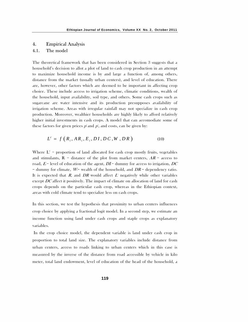
4. Empirical Analysis 4.1. The model The theoretical framework that has been considered in Section 3 suggests that a household’s decision to allot a plot of land to cash crop production in an attempt to maximize household income is by and large a function of, among others, distance from the market (usually urban centers), and level of education. There are, however, other factors which are deemed to be important in affecting crop choice. These include access to irrigation scheme, climatic conditions, wealth of the household, input availability, soil type, and others. Some cash crops such as sugarcane are water intensive and its production presupposes availability of irrigation scheme. Areas with irregular rainfall may not specialize in cash crop production. Moreover, wealthier households are highly likely to afford relatively higher initial investments in cash crops. A model that can accomodiate some of these factors for given prices pc and ps, and costs, can be given by:

( ), , , , , ,=ci i iL f R A R E D I D C W D R

(10)

Where LC = proportion of land allocated for cash crop mostly fruits, vegetables and stimulants, Ri = distance of the plot from market centers, ARi = access to road, Ei = level of education of the agent, DIi = dummy for access to irrigation, DC = dummy for climate, Wi= wealth of the household, and DRi = dependency ratio. It is expected that R, and DR would affect Lc negatively while other variables except DC affect it positively. The impact of climate on allocation of land for cash crops depends on the particular cash crop, whereas in the Ethiopian context, areas with cold climate tend to specialize less on cash crops.

In this section, we test the hypothesis that proximity to urban centers influences

crop choice by applying a fractional logit model. In a second step, we estimate an

income function using land under cash crops and staple crops as explanatory

variables.

In the crop choice model, the dependent variable is land under cash crop in

proportion to total land size. The explanatory variables include distance from

urban centers, access to roads linking to urban centers which in this case is

measured by the inverse of the distance from road accessible by vehicle in kilo

meter, total land endowment, level of education of the head of the household, a


120

dummy for climate, and a dummy for whether a household possesses irrigable

land. Size of own plot, and size of land used under share cropping arrangements

are also considered.

Obviously, OLS procedures are not appropriate when the dependent variable is a ratio bounded between 0 and 1. Running OLS on a fractional dependent variable would entail similar problems as it does in the linear probability model for strict binary cases (Wooldridge, 2002). One of the drawbacks of this approach is that predicted values of OLS estimates would not necessarily lie in the [0,1] interval. The other important advantage of using fractional logit model over OLS is that the first accounts for possible non-linear relationship in the model.

A common approach to model dependent variables which are bounded between 0 and 1 is a logistic transformation where the log-odds ratio is modelled as a linear function of a set of independent variables. Unfortunately such procedure does not account for data that includes the limits 0 and 1. Moreover, it is not possible to recover the predictions for the dependent variable without some simplifying assumptions. In our case, though a value of 1 is rare, there are a number of households who do not allot their plots for cash crop at all. One way out could be to proceed with such transformation by giving an extremely small number for values equal to zero and a near unity number for values of 1. This is, however, arbitrary which may lead to undesirable results (Wooldridge, 2002).

Papke and Wooldridge (1996) based on the results of Gourieroux, Monfort, and Trongen (1984) and McCullagh and Nelder (1989) suggested as an alternative the Generalized Linear Model (GLM) that makes use of quasi-maximum likelihood estimation procedures. The notion of the GLM is that a regression model can be decomposed into a random component with expected value and variance of the dependent variable, a systematic component that is predicted by covariates, and a link function that relates the systematic component to the random component. For classical regression models, the random component is assumed to be distributed normal and the link function is an identity in the sense that the random and systematic components are identical (McCullagh and Nelder, 1989).

What makes GLM more relevant is that the normality assumption on the distribution of the random component could come from any function of the


121

exponential family, and the link function could be any monotonic differentiable function (McCullagh and Nelder, 1989).

Given the dependent variable lc

i and the vector of the various explanatory

variables x, where 0 ≤ lc ≤ 1. Then, for all i:

( )ci iE l x β= (11)

In this case, the random component, ( )ciE l , is expected to have a value of µ so

that 0 ≤ µ ≤ 1, and, unlike the linear regression model, the random component could have a distribution different from normal. It might rather have a binomial distribution which is from the exponential family.

More importantly, the link function cannot be assumed to be identity because the

systematic component ( ix β ) does not ensure the condition that the random

component, ( )ciE l , lies between 0 and 1. Hence, the link function that relates

( )ciE l and ( ix β ) could be given by:

( ) ( )| =ci i iE l x g x β

(12)

where g (.) is a link function satisfying the condition that 0 ≤ g(.) ≤ 1.

Gourieroux, Monfort, and Trongen (1984) showed that quasi-maximum likelihood estimators (QLME)7 are consistent as long as the likelihood function is in the linear exponential family and that the link function under (12) holds. Papke and Wooldridge (1996) suggested the random component to be Bernoulli for it being easy to maximize. For the link function, we use the logistic distribution as suggested by McCullagh and Nelder (1999).

Thus, for with a logistic link function, we have:

7 Quasi‐maximum likelihood estimators, also known as pseudo‐maximum likelihood estimators, are methods which maximize probability distributions which do not necessarily contain the true distribution.


122

( ) ( )1

≡ Λ =+⎡ ⎤⎣ ⎦

i

i

x

i i x

eg x xe

β

ββ β (13)

The Bernoulli likelihood function is given by:

( ) ( ) ( ) 1/ ; 1

c ci il lc

i i i if l x x xβ β β−

= Λ − Λ⎡ ⎤ ⎡ ⎤⎣ ⎦ ⎣ ⎦ , where [ ]0,1 .cil ∈

This can be transformed to give:

( ) ( ) ( ) ( )log 1 log 1c ci i i iL l x l xβ β β= Λ + − − Λ⎡ ⎤ ⎡ ⎤⎣ ⎦ ⎣ ⎦ , (14)

The other model considered in this section is the income function of rural households. The estimable model is given by:

( ), , , , , ,c sr i i hy f L L N O DI E DR=

(15)

where yr = household per capita income from crop production, Lci = land under

cash crop, Lsi = land under staple crop, N = labor, O = number of oxen, DI =

dummy for availability of irrigable land, Eh = education level of the head of the household, and DR = dependency ratio. The model in Equation (15) is estimated by OLS.

4.2 The data and estimation results As it has been introduced in Section 2, the data used for this study is the household survey data collected from six villages in Wollo, the Amhara Regional State. The survey was conducted in the year 2006. The villages were systematically selected based on their distance from major towns. 252 households were randomly selected from the villages. In the crop choice model, distance from town is approximated by the distance in kilometer between what is thought to be ‘centroid’ of the village to the nearest district town. Distance from road is the distance in kilometer of the village from the nearest road accessible by vehicles. We defined access to road as the inverse of the distance from the nearest road accessible by vehicle.


123

Table 1: List of Variables used in the Estimation

Variable Mean Standard Deviation Min Max

Land under cash crop (ratio to the total) 0.12 0.15 0 1 Town-Distance 11.86 5.51 4 20 Distance from Road 3.39 3.80 1 10 Access to Road (inverse of distance) 0.69 0.39 0.1 1 Dummy Irrigation 0.42 0.50 0 1 Dummy Climate (=1 if Dega) 0.29 0.46 0 1 Education - Head

Years of Schooling 2.06 2.99 0 11 Primary (1-6) 0.43 0.50 0 1 Junior Secondary (7-8) 0.06 0.23 0 1 Senior Secondary (9-12) 0.03 0.17 0 1

Total Own Land in hectare 0.72 0.39 0 2.5 Land Leased in for share cropping (LSC1) 0.21 0.38 0 3

Land Leased out for share cropping (LSC2)

0.02 0.10 0 0.75

Dependency Ratio 0.77 0.80 0 4 Permanent Cash Income (per capita) 30.92 157.57 0 1600 Value of Livestock (per capita) 1220.42 1349.76 0 9250 Per Capita Income (logs) 6.68 0.85 0.37 8.77 Land under cash crop 0.11 0.14 0.00 0.50 Land under staple crop 0.72 0.41 0.09 2.25 Labor 2.33 1.02 1 7 Oxen 1.61 1.25 0 9 Cattle (other than oxen) 2.47 2.47 0 12 Dummy Rural Enterprise 0.19 0.40 0 1

The dummy variable for availability of irrigation scheme takes a value of 1 if the village has access to irrigation facilities (modern or traditional) at a significant scale and 0 otherwise. The dummy for climate assumes a value of 1 if the village has cold (dega) climate which in this case ranges from 2600-2800 meters above sea level in elevation and 0 if it has moderate (woina-dega) climate. The elevation in the latter category ranges from 1400 meter for Girana to 1800 meter for Habru-Ligo.

Per capita cash income and per capita value of livestock8 are included to capture the impact of wealth on crop choice. To account for liquidity constraints, we include per capita value of permanent cash income which includes pensions, permanent remittances, and salaries from long-term off-farm employments. Value

8 Similarly, Dercon (1996), and Kurosaki and Fafchamps (2002) used the value of livestock as a proxy for liquid wealth in their crop choice model.


124

of livestock is the sum of the average market price of cattle, goats, sheep, and camels. Livestock ownership may have two opposing impacts on crop choice. On one hand, livestock serve as buffer stock against risk in which case it favors the allocation of more land for cash crop production. On the other hand, livestock farming might be a competing activity to cash crop production. The relative importance of the two effects depends on village specific factors such as distance from urban centers. To disentangle the two effects, we used an interaction variable of distance from urban centers and value of livestock.

For the educational attainment of the head of the household, years of schooling by level (primary, junior secondary and senior secondary levels in which the head has attended some classes) were considered. The maximum year of schooling is 11 years. A dummy is used for each level where a value of 1 denotes some education at the respective level and 0 otherwise. The omitted category is ‘never attended any of these levels’. Own land is the size of plot in hectares that belongs to the household. Size of land under sharecropping arrangements is also included as well as a dummy for whether a household has some plots of land that is adapted to irrigation irrespective of whether the plot is irrigated during the survey period. Many households implanted irrigation schemes but do not necessarily irrigate their plots depending on the season and the type of crop.

A potential source of endogeneity bias arises from liquid assets. Non-agricultural cash income is exogenous because pensions, remittances, and compensations for long term off-farm activities may not be expected to be affected by crop choice decisions. However, the simultaneity problem may arise in the case of value of livestock. Dercon (1996) reports simultaneity between crop choice and value of livestock. On the other hand, Kurosaki and Fafchamps (2002) find that liquid assets and livestock are predetermined and conclude that these variables are exogenous.

In our case we applied a Hausman test to check whether value of livestock is exogenous9. The instruments used were total land size, number of oxen, and labor. The test does not support the null that value of livestock is endogenous.

9 We estimated an auxiliary regression where per capita value of livestock was regressed on total land, labor, and oxen. PCVL = 848.03 + 719.36Land + 349.80Oxen – 304.89Labor (3.68) (3.50) (5.46) (‐4.07) We estimated the crop choice model by including the residual of the auxiliary regression along with the per capita value of livestock (Wooldridge 2002). We found that the coefficient of the residual term was not statistically significant indicating that the case of simultaneity is not supported.


125

4.2.1 Results for crop choice model

The results for the land allocation model are shown in Table 2. In most cases, slopes of the GLM estimates and OLS parameter estimates are not very different both in terms of magnitude and their statistical significance. The results show that proximity to town, access to road, education of the head, ownership of liquid assets and access to irrigation scheme are significant for predicting household crop choices. Rural households under study who operate nearer to urban centers tend to allot more land for the production of cash crops while those households who operate far from urban centers tend to allocate much of their land for the production of staple crops (grains). This might be due to the fact that rural peasants nearer to urban centers have a greater advantage in terms of transportation cost and information about the market. These results support the argument that for crop choices the location of the village relative to the next market matters.

Table 2: GLM Estimation of Land Allocation Decisions

Dependent Variable: Share of Land Allotted to Cash Crop GLM Estimates

OLS Estimates Coefficient Slope

Distance-Town -0.180 [-5.92]*** -0.013 (-6.22) 0.011 (-4.12) [-4.50] Access to Road 1.689 [5.64]*** 0.125 (5.42) 0.091 (3.20) [3.21] Dummy Irrigation 0.787 [2.51]** 0.062 (2.56) 0.067 (3.02) [2.66] Dummy Climate -1.585 [-3.78]*** -0.094 (-3.97) -0.140 (-4.47) [-3.41] Cash Income 0.0009 [3.21]*** 7×10-5 (2.89) 0.0002 (3.07) [2.33] Livestock (Value) -0.0005 [-3.08]** -4×10-5 (-3.08) -4×10-5 (-2.82) [-3.56] VLS×r 5×10-5 [3.21]*** 3.4×10-6 (3.26) 3.5×10-6 (2.33) [3.11] Education-Head Primary (1-6) 0.391 [2.43]*** 0.030 (2.31) 0.032 (1.86) [1.95] Junior Sec. (7-8) 0.904 [2.65]** 0.094 (1.94) 0.103 (2.94) [2.43] Senior Sec.(9-12) 0.398 [0.97] 0.035 (0.83) 0.048 (0.98) [1.15] Total Own Land 0.185 [0.89] 0 .014 (0.91) 0.013 (0.59) [0.58] LSC1 -0.206 [-1.07] -0.015 (-1.05) -0.038 (-1.62) [-2.01] LSC2 0.817 [1.80]* 0.061 (1.79) 0.144 (1.69) [1.59] Dependency Ratio -0.243 [-1.89]* -0.018 (-1.85) -0.022 (-2.14) [-2.09] Intercept -1.375 [-2.48]** - 0.201 (3.55) [3.44] N 252 R2 0.39

2R 0.35 Joint Stability F(14,237) 10.59 21.48

Heteroscedasticity χ2 (1) = 26.50

*** Significant at 1% level, ** Significant at 5% level, * Significant at 10% level. Figures in brackets are t-ratios and those in square brackets are robust t-ratios.


126

The irrigation dummy is significant and positive. Irrigation may have two impacts. First, most cash crops which have high demand in the urban market require a sustainable supply of water. As it has been indicated in Section 2.3, major cash crops that are produced include sugarcane, and fruits whose production is water intensive. Secondly, availability of irrigation scheme gives households the opportunity to produce more than once within a year. This in turn secures them to shift into the production of staple crops with low gestation period during a risk of falling prices of cash crops such as vegetable.

In the case of liquid asset, estimation results without the interaction variable

(VLS×r), value of livestock was found to be insignificant while permanent cash income reveals a positive and significant coefficient. Upon the introduction of the interaction variable, both permanent cash income and value of livestock were significant the latter having a negative coefficient. The interaction variable itself has a positive and significant coefficient.

It can be shown from the coefficients of value of livestock and interaction variables that within about 18 kilometers radius from market centers, the rivalry effect of cash crop production and livestock farming dominates10. Beyond 18 kilometers radius, the role of livestock as a buffer stock against risk dominates in that households with more livestock tend to allot land for cash crop. One explanation for positive association between cash crop production and value of livestock might be that remote villages have significant land that is not arable but which can be used for livestock farming. Hence, livestock farming does not necessarily compete with crop production in terms of land use.

In general, education of the head is positively associated with a higher probability of allocating more land to cash crops. Education on primary and junior secondary levels has positive impact. However, additional schooling to senior secondary schooling does not have much influence on the household’s decision to allot more land to cash crops. The negative sign of the dummy for climate shows that highlanders of the villages under survey do not allot much land to cash crop compared to lowlanders. The coefficients and slopes for total own land, and land under sharecropping arrangements are not statistically significant. Land leased out in the form of share cropping arrangements is significant only at 10 percent level of significance.

10 We calculated the threshold distance (= 18 km) by differentiating the land allocation equation with respect to value of livestock and set to zero. We used the slope coefficients of the GLM estimates for this purpose.


127

Lastly, the dependency ratio (proportion of members of a household below the age of 10 and above the age of 65 to the active labor force) is found to be significant only at 10 percent level in the case of GLM estimation but significant at 5 percent in the case of OLS estimates. Households with a higher share of dependants might be more risk averse and hence do not tend to allot more land for cash crop as they prefer food security. 4.2.2 Results for incomes function To investigate whether distance predicts income we use annual per capita income in Birr from agricultural activities, in particular cash and staple crop production as the dependent variable. On the right hand side we include the distance variables along with size of land under cash crop and staple crops as separate variables as well as a number of further controls. Head counts are used for oxen. In the case of labor, a sort of adult equivalent labor is used. Household members aged 16 and above are given a weight of 1 while those in the age of 10 to 15 are given a weight of 0.5. Some variables which were used as determinants of land allocation decision are also used in estimating the income function. The rationale of including the variables which were used as determinants of land allocation decision (dummy for irrigation scheme, and education) is to see their direct effect on income apart from their impact on it through land allocation decision. Results are summarized in Table 3. The null for constant variance under the Breusch-Pagan test for heteroscedasticity was rejected at 5 percent level. However, there was little change in the standard errors between the OLS and robust estimates causing no change in significance of coefficients at 5 percent level. The estimates revealed that coefficient for land under cash crop was significantly greater than that of the land under staple crop reflecting that the marginal product of land under cash crop is greater compared to its alternative use of staple crop production. More importantly, distance from the nearest urban center is found to significantly predict the level of per capita income of households. It shows that, other things being equal, households operating far from urban centers tend to have lower per capita income compared to those households nearer to towns.


128

Table 3: OLS Results of Rural Per Capita Income: Land being instrumented

Dependent Variable: Per capita Household Income (in logs) Covariates Coefficients t-ratios

Land under cash crop(Estimated) 1.13 (2.13) [3.11] Land under staple crop (Estimated) 0.46 (3.42) [3.22] Labor -0.10 (-2.35) [-2.47] Oxen 0.16 (4.12) [4.21] Dummy for Irrigation 0.36 (3.20) [3.67] Distance from Town -0.03 (-3.15) [-3.31] Access to Road 0.32 (2.20) [2.56] Education - Head Primary (1-6) 0.02 (0.27) [0.28] Junior (7-8) 0.17 (0.86) [0.79] Secondary (9-12) -0.06 (-0.23) [-0.43] Dummy for Rural Enterprise 0.31 (0.89) [3.30] Dummy food for Work 0.09 (3.04) [1.01] Intercept 6.11 (24.00) [23.72] N 252 R2 0.49

2R 0.47 F( 12, 239) 19.28 29.43 RESET: F(3, 236) 1.28 Heteroscedasticity: χ2(1) 4.28

Figures in brackets are t-ratios and those in square brackets are robust t-ratios

5. Conclusions In this article, we investigated the interaction between distance to markets and crop choice in Ethiopia. We found that proximity to urban centers and access to roads increases the share of land allotted to cash crop production. Shorter ways of bringing the produce to the market imply lower transaction costs and consequently better returns. Another channel through which market proximity may affect crop choices is better access to information about prices or new technologies. Furthermore, households located closer to urban centers with access to road but who do not have irrigable land tend to invest in commercial livestock farming and fast growing trees such as eucalyptus to be sold in urban centers. This translates into uneven levels of per capita income among villages: a typical household in the richest village nearer to urban center has a per capita income more than 4 times that of a typical household who lives in the remotest village among those covered by the study.


129

Estimation results of the income function of rural household show that size of plots under cash crops and staple crops are significantly related to higher incomes. The coefficient of land under cash crop is by far greater than that of land under staple crop. Distance from the nearest urban center is found to be significant and negative in the incomes function implying that level of per capita income varies over such distances where the households with relative proximity to urban centers are better off. In conclusion, strong linkages to the urban sector matter for the development prospects of rural areas. Policies that target on supply bottlenecks in the agricultural sector might not be successful without vibrant urban centers which constitute sustainable demand for marketable surplus. In a rural economy such as that of Ethiopia which is characterized by fragmented and static urban enclaves, encouraging township could be considered as a priority. Moreover, enabling rural households to have access to road and better information networking, expanding purposeful education, developing irrigation schemes, introducing new varieties of high yield cash crops including for cold climate zones might help rural households better cope up with shocks and enable them to create surplus that would serve as a basis for agrarian transformation.


130

References Ayalew, Daniel. 2003. Essays on Household Consumption and Production Decisions

under Uncertainty in Rural Ethiopia, Ph.D. Dissertation, Katholieke Universiteit Leuven.

Becker, S. Gary. 1993. Human Capital: A Theoretical and Empirical Analysis with Special Reference to Education, The University of Chicago Press.

CSA: Central Statistical Agency of the Federal Democratic Republic of Ethiopia, Annual Statistical Abstract, Various Issues.

Dercon, Stefan. 1996. “Risk, Crop Choice and Savings: Evidence from Tanzania,” Economic Development and Cultural Change, Vol. 44, No. 3, pp. 485-514.

Dillon, John L. and Pasquale L. Scandizzo. 1978. “Risk Attitudes of Subsistence Farmers in Northern Brazil: A Sampling Approach,” American Journal of Agricultural Economics, Vol. 60, No. 3, pp. 425-435.

Fafchamps, Marcel. 1992. “Cash Crop Production, Food Price Volatility, and Rural Market Integration in the Third World,” American Journal of Agricultural Economics, pp. 90-99.

Fafchamps, Marcel and Agnes R. Quisumbing. 1999. “Human Capital, Productivity, and Labor Allocation in Rural Pakistan,” The Journal of Human Resources, Vol. 34, No. 2, pp. 369-406.

Fujita, Masahisa and Jacques-Francois Thisse. 1986. “Spatial Competition with a Land Market: Hotelling and Von Thunen Unified.” The Review of Economic Studies, Vol. 53, No. 5, pp. 819-841.

_______. 2002. Economics of Agglomeration: Cities, Industrial Location, and Regional Growth, Cambridge University Press.

Gourieroux, C. A. Monfort and A. Trognon. 1984. “Pseudo Maximum Likelihood Methods: Theory,” Econometrics, Vol. 52, No. 3, pp. 681-700.

Haddad, Lawrence, John Hoddinott, and Harold Alderman. 1997. Intrahousehold Resource Allocation in Developing Countries. The Johns Hopkins University Press.

Jones, Charles I. 2003: Introduction to Economic Growth, New York, W.W. Norton and Co. Second Edition.

_______. 2004. Growth and Ideas, NBER Working Paper No. 10767. Kurosaki, Takashi and Marcel Fafchamps. 2002. “Insurance Market Efficiently and Crop

Choices in Pakistan,” Journal of Development Economics, Vol. 67, No. 2, pp. 419-453.

McCullagh, P. and J. A. Nelder. 1999. Generalized Linear Models; Monographs on Statistics and Applied Probability 37, Second Edition, Chapman & Hall/CRC

MoFED. 2011. Ministry of Finance and Economic Development, National Income Account

Nerlove, Mark L. and Efraim Sadka. 1991. “Von Thunen's Model of the Dual Economy.” Journal of Economics, Vol. 54, N0. 2, pp. 97-123.


131

Papke, Leslie E. and Jeffery M. Wooldridge. 1996. "Econometric Methods for Fractional Response Variables with an Application to 401 (K) Plan Participation Rates." Journal of Applied Econometrics, Vol. 11, No. 6, pp. 619-632.

Pindyck, Robert S. and Daniel L. Rubinfeld. 1998. Econometric Models and Econometric Forecasts; Forth Edition, Irwin Mc Graw-Hill

Ray, Debraj. 1998. Development Economics, Princeton University Press. Samuelson, Paul A. 1983. "Thunen at Two Hundred." Journal of Economic Literature,

Vol. 21, No. 4, pp. 1468-1488. Wooldridge, Jeffery M. 2002. Econometric Analysis of Cross Section and Panel Data;

The MIT Press, Cambridge, Massachusetts.

the impact of proximity to urban center on … nuru... · seid nuru and holger seebens: the impact...

Documents