synthetic seismograms and seismic waveform...
TRANSCRIPT

Synthetic Seismograms andSeismic Waveform Modeling
Lupei ZhuSaint Louis University
2011

c©Copyright byLupei Zhu
ALL RIGHTS RESERVED2001–2011
i

Acknowledgments
I am grateful to many graduate students, including Sebastiano d’Amico, Ali Fatehi, JuliaKurpan, Filipe Leyton, Oner Sufuri, Yan Xu, Hongfeng Yang, and Kathy Zou, at Departmentof Earth and Atmospheric Sciences, Saint Louis University, who helped to correct numerouserrors and typos and to improve the notes.
ii

Contents
1 Introduction 1
1.1 Characteristics of seismic waveforms in different distance ranges . . . . . . . 1
1.2 Seismic instruments and seismic data processing . . . . . . . . . . . . . . . . 2
1.2.1 Seismic instrument response . . . . . . . . . . . . . . . . . . . . . . . 2
1.2.2 Digital signal processing . . . . . . . . . . . . . . . . . . . . . . . . . 3
1.3 Exercises . . . . . . . . . . . . . . . . . . . . . . . . . . . . . . . . . . . . . . 4
2 Seismic Sources 5
2.1 Seismic sources . . . . . . . . . . . . . . . . . . . . . . . . . . . . . . . . . . 5
2.1.1 Seismic source representation . . . . . . . . . . . . . . . . . . . . . . 5
2.1.2 Ideal fault . . . . . . . . . . . . . . . . . . . . . . . . . . . . . . . . . 6
2.1.3 Decompositions of a general moment tensor . . . . . . . . . . . . . . 7
2.1.4 DC moment tensor components . . . . . . . . . . . . . . . . . . . . . 9
2.2 Displacements produced by a point source in a whole-space . . . . . . . . . . 10
2.2.1 A single-force source . . . . . . . . . . . . . . . . . . . . . . . . . . . 10
2.2.2 A general moment tensor source . . . . . . . . . . . . . . . . . . . . . 12
2.2.3 Examples . . . . . . . . . . . . . . . . . . . . . . . . . . . . . . . . . 13
2.3 Exercises . . . . . . . . . . . . . . . . . . . . . . . . . . . . . . . . . . . . . . 14
3 Multi-layered Media – Generalized Ray Theory 18
iii

3.1 Solution to wave equation in cylindrical coordinate system . . . . . . . . . . 18
3.2 A liquid whole-space . . . . . . . . . . . . . . . . . . . . . . . . . . . . . . . 19
3.3 Two liquid half-spaces . . . . . . . . . . . . . . . . . . . . . . . . . . . . . . 21
3.4 A sandwiched liquid layer between two liquid half-spaces . . . . . . . . . . . 23
3.5 Double-couple sources in elastic media . . . . . . . . . . . . . . . . . . . . . 25
3.6 Exercises . . . . . . . . . . . . . . . . . . . . . . . . . . . . . . . . . . . . . . 29
4 Multi-layered Media – Frequency-Wavenumber Integration Method 31
4.1 Displacement-stress vector in a source-free homogeneous medium . . . . . . . 31
4.2 Surface displacement of layered half-space from an embedded point source . 34
4.3 Source terms and horizontal radiation pattern . . . . . . . . . . . . . . . . . 38
4.3.1 Explosion source . . . . . . . . . . . . . . . . . . . . . . . . . . . . . 38
4.3.2 Single force . . . . . . . . . . . . . . . . . . . . . . . . . . . . . . . . 38
4.3.3 Double-couple without torque . . . . . . . . . . . . . . . . . . . . . . 39
4.4 Frequency-wavenumber integration . . . . . . . . . . . . . . . . . . . . . . . 39
4.4.1 Wavenumber integration . . . . . . . . . . . . . . . . . . . . . . . . . 40
4.4.2 Compound matrix . . . . . . . . . . . . . . . . . . . . . . . . . . . . 44
4.4.3 Other boundary conditions . . . . . . . . . . . . . . . . . . . . . . . . 45
4.4.4 Buried receivers . . . . . . . . . . . . . . . . . . . . . . . . . . . . . . 45
4.4.5 Partitioning of up-going and down-going wavefields . . . . . . . . . . 46
4.4.6 Some practical aspects in the F-K integration . . . . . . . . . . . . . 46
4.5 Differential seismograms . . . . . . . . . . . . . . . . . . . . . . . . . . . . . 52
4.5.1 Analytical derivatives of propagator matrices and source terms . . . . 52
4.5.2 Analytical solution . . . . . . . . . . . . . . . . . . . . . . . . . . . . 52
4.5.3 Implementation and tests . . . . . . . . . . . . . . . . . . . . . . . . 52
4.5.4 Application to waveform inversion . . . . . . . . . . . . . . . . . . . . 52
iv

4.6 Exercises . . . . . . . . . . . . . . . . . . . . . . . . . . . . . . . . . . . . . . 53
5 Regional Distance Seismic Waveforms 54
5.1 Local distances . . . . . . . . . . . . . . . . . . . . . . . . . . . . . . . . . . 54
5.2 Regional distances . . . . . . . . . . . . . . . . . . . . . . . . . . . . . . . . 54
6 Upper-mantle Distance Waveforms 66
6.1 Earth flattening transformation . . . . . . . . . . . . . . . . . . . . . . . . . 66
6.2 Velocity discontinuity and triplication . . . . . . . . . . . . . . . . . . . . . . 73
6.3 Upper-mantle structure from modeling triplicated waveforms . . . . . . . . . 73
7 Teleseismic Waveforms 74
7.1 Computing teleseismic synthetics . . . . . . . . . . . . . . . . . . . . . . . . 74
7.1.1 Full waveforms using normal-mode summation, DSM, and FK . . . . 74
7.1.2 Construction of teleseismic P -wave with GRT . . . . . . . . . . . . . 74
7.2 Determining earthquake moment tensors and focal depth . . . . . . . . . . . 74
7.3 Determine upper mantle structure . . . . . . . . . . . . . . . . . . . . . . . . 74
7.4 Teleseismic receiver functions . . . . . . . . . . . . . . . . . . . . . . . . . . 74
7.4.1 Computing receiver functions . . . . . . . . . . . . . . . . . . . . . . 76
7.4.2 Inversion for 1-D velocity structure . . . . . . . . . . . . . . . . . . . 79
7.4.3 Estimate crustal thickness and Vp/Vs ratio . . . . . . . . . . . . . . . 79
7.4.4 CCP stacking and imaging . . . . . . . . . . . . . . . . . . . . . . . . 81
7.5 Core phases . . . . . . . . . . . . . . . . . . . . . . . . . . . . . . . . . . . . 81
7.6 Exercises . . . . . . . . . . . . . . . . . . . . . . . . . . . . . . . . . . . . . . 82
Bibliography 94
v

List of Figures
1.1 Example observations and synthetics at ranges where the Earth appears sim-ple (>30◦), slightly complicated (upper-mantle ranges, 30◦ to 14◦) and quitecomplicated (<14◦), from [Helmberger, 1983]. . . . . . . . . . . . . . . . . . 1
1.2 Spectral amplitudes of ambient seismic noise, earthquakes (magnitude 5 and9 recorded at a distance of 4,500 km), and Earth tides. . . . . . . . . . . . . 3
2.1 Moment tensor elements and their corresponding force dipoles and couples(from Aki and Richards [1980]). . . . . . . . . . . . . . . . . . . . . . . . . 6
2.2 P and T axes of a double couple moment tensor. . . . . . . . . . . . . . . . 7
2.3 The ISO-DC-CLVD diagram showing permissible values of the ΛISO, ΛCLVD,and ΛDC percentages as bounded by the outer diamond. The pure explosionand implosion sources are indicated by the circles. The pure DC source islocated at the center. The contours show DC levels of 75% and 50%. . . . . 10
2.4 Displacement u from a single force F in a whole-space. Waveform shapes ofthe near field, far-field P , and far-field S are shown on the right. . . . . . . 11
2.5 Radiation patterns and particle motions of far-field P (left) and S from asingle force. . . . . . . . . . . . . . . . . . . . . . . . . . . . . . . . . . . . . 12
2.6 Displacement u produced by a double couple in the x1-x3 plane. . . . . . . 13
2.7 Radiation patterns and particle motions of far-field P (left) and S from adouble couple. . . . . . . . . . . . . . . . . . . . . . . . . . . . . . . . . . . 13
2.8 The bottom trace is the vertical-component acceleration recorded by TriNetstation TAB from a nearby Mw 4.2 earthquake (3 km away and at a depth of11 km). The top trace in black is the obtained displacement waveforms usingdouble integration. The red-colored trace is synthetic displacement using thewhole-space solution (multiplied by 2 to account for the free-surface effect). 14
vi

2.9 Black-colored traces are three-component displacement waveforms recorded atthe BANJO array from the 1994 Mw 8.3 Bolivia deep earthquake (from Zhu[2003]). Red-colored traces are synthetic displacements using the whole-spacesolution (multiplied by 2 to account for the free-surface effect). . . . . . . . 15
2.10 Observation of near field at teleseismic distances from the 1994 Bolivia deepearthquake (from Vidale et al. [1995]). . . . . . . . . . . . . . . . . . . . . . 16
3.1 Cagniard-de Hoop contour. . . . . . . . . . . . . . . . . . . . . . . . . . . . 20
3.2 Two liquid half-spaces. . . . . . . . . . . . . . . . . . . . . . . . . . . . . . 21
3.3 Cagniard contour for reflection ray in two liquid half-spaces. . . . . . . . . . 23
3.4 Vertical displacements produced by an explosion in a two liquid half-spacemodel, located 5 km above the contact interface. The P velocity in the tophalf-space is 5 km/s, and 7.5 km/s in the bottom half-space. . . . . . . . . . 24
3.5 Vertical displacements from a strike-slip fault at 5 km depth in a uniformhalf-space (Vp 6.3 km/s, Vs 3.6 km/s, and ρ 2.7 g/cm3). . . . . . . . . . . . 28
4.1 A layered half-space consists of N layers over a half-space at the bottom. Thesource is located at a depth of h between layer m and m + 1 with identicalelastic properties. . . . . . . . . . . . . . . . . . . . . . . . . . . . . . . . . 34
4.2 Raleigh denominator (ω = 1 Hz) and locations of branch points and Rayleighpole for a half space (α=6.3 km/s, β=3.5 km/s). Note that the Rayleigh poleis on the right of kβ which means that Rayleigh velocity is slower than theshear velocity of the half space. . . . . . . . . . . . . . . . . . . . . . . . . . 37
4.3 Love denominator as function of wavenumber (we set ω = 3 Hz) for a onelayer over half space model. Note that there are multiple poles correspondingto fundamental and higher modes and all the poles are located between kβ1
and kβ2 . . . . . . . . . . . . . . . . . . . . . . . . . . . . . . . . . . . . . . . 37
4.4 Location of branch points and poles in complex k-plane. . . . . . . . . . . . 40
4.5 Vertical displacement kernel as function of k for different Qβ and σ value (weset ω = 0.47 Hz). The velocity model is a one-layer over half-space, withα1 = 6.3, β1 = 3.5, α2 = 8.1, β2 = 4.5. . . . . . . . . . . . . . . . . . . . . . 41
4.6 F-K integrand U(ω, k)J0(kx) at distance ranges of 100 km (above) and 1000 km(below). . . . . . . . . . . . . . . . . . . . . . . . . . . . . . . . . . . . . . . 42
4.7 Discrete summation in wavenumber is equivalent to summing infinite numberof point sources (open circles) uniformly distributed in r direction. . . . . . . 42
vii

4.8 Bessel function J0(x) (solid line) and its first term of asymptotic expansion√2
πxcos(x− π
4) (dashed line). . . . . . . . . . . . . . . . . . . . . . . . . . . 43
4.9 Components of Greens’ function at distance of 1 km for a double couple sourcein half space (Vp=6.3 km/s, Vs=3.5 km/s, source depth 10 km). The com-ponents are, from the bottom to top, ZDD, RDD, TDD, ZDS, RDS, TDS,ZSS, RSS, and TSS. The near field between P and S arrivals and permanentdisplacements after S are best displayed on ZDD. . . . . . . . . . . . . . . . 48
4.10 Comparison of Greens functions calculated by FK method (heavy lines) withthose by GRT (red lines). The velocity model is a 30-km-thick layer (Vp=6.3 km/sand Vs=3.6 km/s) over a half space (Vp=8.1 km/s and Vs=4.5 km/s). Thesource is at 10 km depth and the distance range is 100 km. The componentsare, from the bottom to top, ZDD, RDD, TDD, ZDS, RDS, TDS, ZSS, RSS,and TSS. Total of 14 primary rays are used in GRT calculation which takesabout 0.1 sec on a SUN-Ultra. FK takes about 1.4 sec. . . . . . . . . . . . . 49
4.11 Greens’ function at distance of 600 km for previous model. Wavenumbersampling interval dk is set to 0.005 km−1. . . . . . . . . . . . . . . . . . . . 50
4.12 Same velocity model and distance range as in Figure 4.11, but shows theproblem of space-aliasing in waveforms when dk is not small enough (dk =0.01 km−1). . . . . . . . . . . . . . . . . . . . . . . . . . . . . . . . . . . . . 51
5.1 Comparison of synthetics with strong-motion record of station IVC of anearthquake at Brawley, CA, in Nov. 1976. From Helmberger [1983]. . . . . 55
5.2 Intermediate depth earthquakes in southern Tibet. . . . . . . . . . . . . . . 56
5.3 SH displacement profile of event 355. . . . . . . . . . . . . . . . . . . . . . . 57
5.4 SH components of Green’s function at different source depths. . . . . . . . . 58
5.5 Comparison of LHSA vertical and radial records with synthetics. . . . . . . . 59
5.6 Vertical components of motion as a function of number of generalized raysummed. The epicentral distance is 1000 km. From Helmberger [1983]. . . . 60
5.7 Profile of vertical displacements for the three fundamental faults. The Green’sfunctions have been convolved with a 1.5 s trapezoid source time function.From Helmberger [1983]. . . . . . . . . . . . . . . . . . . . . . . . . . . . . 61
5.8 Profile of vertical displacement for the three fundamental faults. The Green’sfunctions have been convolved with a 3 s trapezoid source time function anda WWSSN long-period instrument response. From Helmberger [1983]. . . . 62
viii

5.9 The vertical Pnl waveforms of the 1966 Truckee earthquake. The strike-slipfocal mechanism (strike 43◦N, dip 76◦SE, and rake -11◦) of the event has twonodal planes which project through station TUC and BOZ. From Helmberger[1983]. . . . . . . . . . . . . . . . . . . . . . . . . . . . . . . . . . . . . . . . 63
5.10 Filtered data and synthetics from the Oroville earthquake. At all stationsexcept GOL both the vertical (the first trace pair) and radial componentsare shown. The focal mechanism (strike 204◦, dip 66◦, rake 275◦) generatespositive first-motions at all station in regional distances as opposed to thoseobserved teleseismically. From Helmberger [1983]. . . . . . . . . . . . . . . 64
5.11 Filtered data and synthetics for both the vertical and radial components froman earthquake in Turkey (strike 131◦, dip 68◦, rake 272◦). From Helmberger[1983]. . . . . . . . . . . . . . . . . . . . . . . . . . . . . . . . . . . . . . . . 65
6.1 IASPEI91 upper-mantle seismic velocity model before the Earth flatteningtransformation (red lines) and after (black lines). . . . . . . . . . . . . . . . 67
6.2 Direct, reflected and head waves for a two liquid half-space model. . . . . . 68
6.3 P (left) and SH (right) triplicated waveforms due to the 410 discontinuity. 69
6.4 Triplicated P (left) and SH (right) waveforms for the IASPEI91 velocitymodel. . . . . . . . . . . . . . . . . . . . . . . . . . . . . . . . . . . . . . . 70
6.5 Vertical component seismograms going from Pnl domination at regional dis-tances to P and long-period at intermediate distances, a) strike-slip and b)dip-slip. . . . . . . . . . . . . . . . . . . . . . . . . . . . . . . . . . . . . . . 71
6.6 Comparison of synthetics with data of 9/12/1966 Truckee earthquake (strike48◦, dip 80◦, and rake 0◦) at regional and upper-mantle distances. FromHelmberger [1983]. . . . . . . . . . . . . . . . . . . . . . . . . . . . . . . . . 72
7.1 Vertical component record section of the 1994 Bolivia deep earthquake. . . 75
7.2 IASPEI91 velocity model after EFT. . . . . . . . . . . . . . . . . . . . . . . 76
7.3 Vertical (left) and transverse (right) components of DSM (red) and FK (black)synthetics for the IASPEI91 model. A 20-sec-low-pass filter is applied. . . . 77
7.4 Vertical (left) and transverse (right) components of normal-mode (red) andDSM (black) synthetics for the IASPEI91 model. A 20-sec-low-pass filter isapplied. . . . . . . . . . . . . . . . . . . . . . . . . . . . . . . . . . . . . . . 78
ix

7.5 Teleseismic P -wave synthetics. The source time functions are (0.5, 1.0, 0.5)secs for high stress-drop, (1.0, 3.0, 1.0) secs for medium stress-drop, and (2.0,6.0, 2.0) for low stress-drop. From Helmberger [1983]. . . . . . . . . . . . . 83
7.6 Observed (top) and synthetic (bottom) long-period P waveforms at 14 WWSSNstations from the Borrego Mtn. earthquake. From Helmberger [1983]. . . . 84
7.7 Observed (top) and synthetic (bottom) long-period P waveforms from theOroville earthquake on Aug. 1, 1975 (strike 180◦, dip 65◦, rake -70◦). FromHelmberger [1983]. . . . . . . . . . . . . . . . . . . . . . . . . . . . . . . . . 85
7.8 Observed (top) and synthetic (bottom) vertical long-period WWSSN P wave-forms from the Bermuda earthquake on March 24, 1978. From Helmberger[1983]. . . . . . . . . . . . . . . . . . . . . . . . . . . . . . . . . . . . . . . . 86
7.9 Receiver functions of a one-layer crustal model. The ray parameter of theincident P wave is 0.06 km/s. . . . . . . . . . . . . . . . . . . . . . . . . . . 87
7.10 Teleseismic receiver functions (right) computed from 10 teleseismic eventsrecorded at station PAS (left). . . . . . . . . . . . . . . . . . . . . . . . . . 88
7.11 Inversion results using receiver functions of WNDO from SE. (a) Initial (dashedline) and final (solid line) shear velocity models. (b) the fit of final syntheticreceiver function (dashed line) to both the mean receiver function (solid line)and the bounds (c). . . . . . . . . . . . . . . . . . . . . . . . . . . . . . . . 89
7.12 The left panel shows radial receiver function as a function of ray parameter pfor the Standard Southern California Velocity Model. Right: (a) The s(H, κ)from stacking the receiver functions using (7.10). It reaches the maximum(solid area) when the correct crustal thickness and Vp/Vs ratio are used inthe stacking. (b) H-κ relations, as given in (7.7)–(7.9), for different Mohoconverted phases. Each curve represents the contribution from this convertedphase to the stacking. . . . . . . . . . . . . . . . . . . . . . . . . . . . . . . 90
7.13 (A) The amplitude and variance (given by the contours) of CCP stacking.No vertical exaggeration except that the surface topography is amplified by afactor of 2. SAF: San Andreas Fault; LAB: Los Angeles Basin. (B) Crustalstructure along the profile based on A. The thickened black lines are Moho andother possible velocity discontinuities. SMF: Sierra Madre Fault; VCT: VicentThrust Fault. Red crosses are earthquakes within the profile between 1981 and1998. Green lines are the crustal reflectors imaged by LARSE [Ryberg andFuis, 1998]; Hatched area in the upper mantle represents the Transverse Rangehigh velocity anomaly from seismic tomography [Humphreys and Clayton,1990]. Plotted on the top are the observed Bouguer gravity anomaly and thepredicted Bouguer anomalies using the determined Moho topography (dashedline) and the Airy isostasy model (dotted line). . . . . . . . . . . . . . . . . 91
x

7.14 Vertical component of GRT synthetic seismograms for the IASPE91 model. 92
7.15 Comparison between observed (red) and synthetic vertical component of ve-locity records from the 6/29/2001 Mw 6.1 earthquake. . . . . . . . . . . . . 93
xi

Chapter 1
Introduction
1.1 Characteristics of seismic waveforms in different
distance ranges
Figure 1.1: Example observations and synthetics at ranges where the Earth appears simple(>30◦), slightly complicated (upper-mantle ranges, 30◦ to 14◦) and quite complicated (<14◦),from [Helmberger, 1983].
1

Table 1.1: Instrument constants of different seismometersSTS-1 STS-2 CMG-3ESP CMG-40T FBA-23 Episensor
f0, Hz 2.7778×10⁻³ 8.3333×10⁻³ 8.3333×10⁻³ 3.3333×10⁻² 50 180G 2500 V/m/s 1500 V/m/s 2000 V/m/s 800 V/m/s 5 V/g 10 V/g
1.2 Seismic instruments and seismic data processing
1.2.1 Seismic instrument response
The output y(t) of a simple vertical seismometer consisting of a spring k and a dash boardη in response to ground motion x(t) can be described by:
my = −ky − ηy +mGx (1.1)
ory + 2hω0y + ω2
0y = Gx, (1.2)
where ω0 =√k/m (natural frequency of the spring), h = η/2
√mk (damping constant), and
G is the amplification factor. Essentially, the response of a simple mechanical seismometeris determined by these three constants.
The frequency response of the seismometer is
H(ω) =Y (ω)
X(ω)=
Gω2
ω2 − 2ihω0ω − ω20
. (1.3)
Responses of modern broadband seismometers such as STS-1 and STS-2 take the same formas above, but are often responses to ground velocity instead of displacement. Accelerometers(e.g. FBA) respond to ground acceleration. Their responses are in the form
H(ω) =−Gω2
0
ω2 − 2ihω0ω − ω20
, (1.4)
with a very large ω0 (50 to 180 Hz) so that the response is essentially flat at G for ω � ω0.
The analog output of a seismometer, normally in the unit of volts, is converted intodigital counts by the data logger, which also applies a low-pass filter to the signal to avoidsampling aliasing. A 24-bit data logger has a dynamic range of 224 = 144 dB. For exam-ple, the Quantera Q680’s digitization constant is 223 counts/20 V and the K2’s constant is223 counts/2 V.
The frequency and dynamic ranges of several popular seismometers are shown in Fig. 1.2.
Often an instrument response is expressed in terms of poles and zeros using z-transform:
H(z) = A0
∏j(z − zj)∏j(z − pj)
, (1.5)
where z = iω. For example, the two poles for the response in Eq. 1.3 are ω0(−h± i√
1− h2).
2

Figure 1.2: Spectral amplitudes of ambient seismic noise, earthquakes (magnitude 5 and 9recorded at a distance of 4,500 km), and Earth tides.
1.2.2 Digital signal processing
The output of a seismic instrument is the convolution of input x(t) and instrument response:
y(t) = h(t) ∗ x(t) =
∫ ∞
−∞h(τ − t)x(τ)dτ. (1.6)
Removing instrument response in y(t) (deconvolution) can therefore be done either in thefrequency domain using spectrum division in the time domain by solving a linear equationsystem.
3

1.3 Exercises
1. Use program stp to retrieve waveforms of seismic station TAB from a M4.4 earthquakeon Aug. 20, 1998, near the San Andreas Fault (event CUSP ID 9064568).
2. According to documentation (see www.data.scec.org/stations/seed/dl seed.php), chan-nel HHZ is from a Guralp CMG-40T sensor and channel HLZ is from a FBA-23 sensor.Remove instrumental responses in these two channels to obtain vertical displacementwaveform at TAB.
3. Plot and compare the displacement waveforms from these two sensors.
4

Chapter 2
Seismic Sources
2.1 Seismic sources
2.1.1 Seismic source representation
Earthquakes and other indigenous sources can be considered to be the result of a local-ized, transient failure of the linearized elastic constitutive relation. We define the differencebetween the true stress and the modeled stress as the stress glut
S = Tmodel −Ttrue. (2.1)
The equation of motion
ρ∂2u
∂t2= ∇ ·Ttrue, (2.2)
can be re-written as
ρ∂2u
∂t2= ∇ ·Tmodel + f , (2.3)
where f is the seismic source term and is called the equivalent body force:
f = −∇ · S. (2.4)
It can be shown that the net force and torque of f in V are zero.
The seismic moment tensor of the source is defined as
Mij =
∫V
fixjdV =
∫V
SijdV, (2.5)
which is a symmetric tensor. Its diagonal elements correspond to force dipoles and off-diagonal elements correspond to force couples (Fig. 2.1).
5

Figure 2.1: Moment tensor elements and their corresponding force dipoles and couples (fromAki and Richards [1980]).
The scalar moment of the source is defined using the norm of the tensor:
M0 ≡1√2
√MijMij. (2.6)
The factor√
2 was introduced for historical compatibility (see below).
2.1.2 Ideal fault
An ideal fault is a surface Σ embedded within V across which there is a tangential slipdiscontinuity ∆u. So
∆u · n = 0. (2.7)
It can be shown that the stress glut is zero everywhere except on Σ:
S = mδΣ, (2.8)
where m = C : n∆u is the stress-glut density. For an isotropic Earth model:
m = µ∆u(nv + vn), (2.9)
6

n
v
T
P
Figure 2.2: P and T axes of a double couple moment tensor.
which can be shown graphically equivalent to two force couples (double-couple, or DC). Thescalar moment of the source with a fault area of A is
M0 = µ∆uA. (2.10)
A double-couple moment tensor has three eigenvalues: ±M0, 0. The three eigenvectors
T =1√2(n + v), (2.11)
P =1√2(n− v), (2.12)
N = n× v, (2.13)
are called the tension axis (T -axis, corresponding toM0), the pressure axis (P -axis,correspondingto −M0), and the null axis (N -axis, corresponding to 0), respectively. Note that the T -axisis located in the compressional quadrants of the focal sphere and the P -axis is located in thedilatational quadrants (Fig. 2.2). They are not principal stress axes.
2.1.3 Decompositions of a general moment tensor
A general moment tensor can be decomposed into an isotropic tensor and a deviatoric tensor:
Mij =1
3tr(M)δij +M ′
ij =√
2M0
(ζIij +
√1− ζ2Dij
), (2.14)
where
Iij =1√3δij, (2.15)
7

is the normalized isotropic tensor and Dij is a normalized deviatoric tensor.
ζ =tr(M)√
6M0
, (2.16)
is a dimensionless parameter ranging from -1 to 1 that quantifies the relative strength of theistropoic component.
Next we decompose Dij into double-couple and CLVD components. The CLVD has adipole of magnitude 2 in its symmetry axis compensated by two unit dipoles in the orthogonaldirections [Knopoff and Randall, 1970]. Let λ1 be the largest eigenvalue (corresponding tothe T -axis eigenvector T) of the deviatoric tensor Dij, λ2 be the intermediate eigenvalue
(corresponding to the null-axis eigenvector N), and λ3 the smallest eigenvalue (correspondingto the P -axis eigenvector P), i.e.,
λ1 ≥ λ2 ≥ λ3. (2.17)
Note that all λi’s are dimensionless and satisfy the conditions
λ1 + λ2 + λ3 = 0, (2.18)
λ21 + λ2
2 + λ23 = 1. (2.19)
Using (2.17)–(2.19), we get
max(λ2) = min(λ1) =1√6, (2.20)
min(λ2) = max(λ3) = − 1√6. (2.21)
When λ2 = 0 the deviatoric tensor Dij is a pure double-couple.
As mentioned, the DC-CLVD decomposition is not unique as the CLVD symmetry axiscan be aligned with any of the principal axes [e.g. Jost and Herrmann, 1989, Hudson et al.,1989]. Here we align the CLVD symmetry axis with the N -axis [e.g. Chapman and Leaney,2011]:
Dij = λ1TiTj + λ2NiNj + λ3PiPj
=λ1 − λ3√
2DDC
ij +
√3
2λ2D
CLVDij ,
(2.22)
where
DDCij =
1√2(TiTj − PiPj), (2.23)
DCLVDij =
1√6(2NiNj − TiTj − PiPj), (2.24)
are normalized DC and CLVD tensors. The above decomposition has the attractive propertythat the DC and CLVD basic sources are orthogonal
DDCij DCLVD
ij = 0. (2.25)
8

The strength of the CLVD component can be quantified by the dimensionless parameter
χ =
√3
2λ2. (2.26)
It can be shown from (2.20) and (2.21) that 12≥ χ ≥ −1
2.
Therefore, one way to parameterize a general moment tensor in terms of the basicisotropic, double couple, and CLVD sources while preserving the total scalar moment is
Mij =√
2M0
(ζIij +
√1− ζ2
(√1− χ2DDC
ij + χDCLVDij
)). (2.27)
The relative strength of each part can be measured by the ratio of its scalar moment to thetotal moment:
ΛISO = sgn(ζ)ζ2, (2.28)
ΛDC = (1− ζ2)(1− χ2), (2.29)
ΛCLVD = sgn(χ)(1− ζ2)χ2, (2.30)
such that|ΛISO|+ ΛDC + |ΛCLVD| = 1. (2.31)
Note that in this decomposition the maximum CLVD is 25% (at ζ = 0 and χ = ±1/2)(Fig. 2.1.3).
2.1.4 DC moment tensor components
With x-axis to the North, y-axis to the East, and z-axis down,
n = (− sin δ sinφ, sin δ cosφ,− cos δ)T , (2.32)
v = (cosλ cosφ+ sinλ cos δ sinφ, cosλ sinφ− sinλ cos δ cosφ,− sinλ sin δ)T , (2.33)
where φ is the fault strike measured from the North, δ is the fault dip measured from thehorizontal, and λ is the slip direction (rake angle) measured CCW from the fault strikedirection. For DC (see A&R, P112):
Mxx = −(sin δ cosλ sin 2φ+ sin 2δ sinλ sin2 φ), (2.34)
Mxy = sin δ cosλ cos 2φ+1
2sin 2δ sinλ sin 2φ, (2.35)
Mxz = −(cos δ cosλ cosφ+ cos 2δ sinλ sinφ), (2.36)
Myy = sin δ cosλ sin 2φ− sin 2δ sinλ cos2 φ, (2.37)
Myz = −(cos δ cosλ sinφ− cos 2δ sinλ cosφ), (2.38)
Mzz = sin 2δ sinλ. (2.39)
9

-ΛCLVD
6ΛISO
DC
75%
50%
u1
e-1
-14
14
@@
@@
@@
��
��
��
@@
@@
��
��
CCCCCCCCCCCC
CCCCCCCCCCCC
������������
������������
Figure 2.3: The ISO-DC-CLVD diagram showing permissible values of the ΛISO, ΛCLVD,and ΛDC percentages as bounded by the outer diamond. The pure explosion and implosionsources are indicated by the circles. The pure DC source is located at the center. Thecontours show DC levels of 75% and 50%.
2.2 Displacements produced by a point source in a
whole-space
2.2.1 A single-force source
The displacement in a uniform whole-space produced by a single force Fp at the origin(Fig. 2.4) is
ui(r, t) =3γiγp − δip
4πρr3
∫ r/β
r/α
τFp(t− τ)dτ +γiγp
4πρα2rFp(t−
r
α) +
δip − γiγp
4πρβ2rFp(t−
r
β), (2.40)
where γi = xi
ris the i-th component of the unit vector r. This is one of the most important
solutions in seismology and was first given by Stokes in 1849. The first term of RHS is calledthe near field because it decays with distant rapidly. The other two terms are called thefar-field P and S wave-fields respectively. When the source time function is an impulse, thefar-field P and S waveforms are impulsive but the near-field waveform is a ramp starting atthe P arrival time and ending at the S arrival time (Fig. 2.4).
If we set up a spherical coordinate system (r,θ,φ) with the symmetry axis aligned with the
10

F
θ
θ
r
o
u
0 1 2 3 4
t (s)
tp ts
Near field
Far−field P
Far−field S
Total
Figure 2.4: Displacement u from a single force F in a whole-space. Waveform shapes of thenear field, far-field P , and far-field S are shown on the right.
single force direction (see Fig. 2.4), the directional variations of far-field P and S displacementamplitudes can be written as
AP = cos θr (2.41)
AS = − sin θθ. (2.42)
It is clear that the particle motion of the far-field P is parallel to r, i.e., the propagationdirection, as expected. Its amplitude varies with direction as cos θ. The particle motion ofthe far-field S is perpendicular to the propagation direction and its amplitude varies withdirection as sin θ. The P - and S-wave source radiation patterns are illustrated in Fig. 2.5.
11
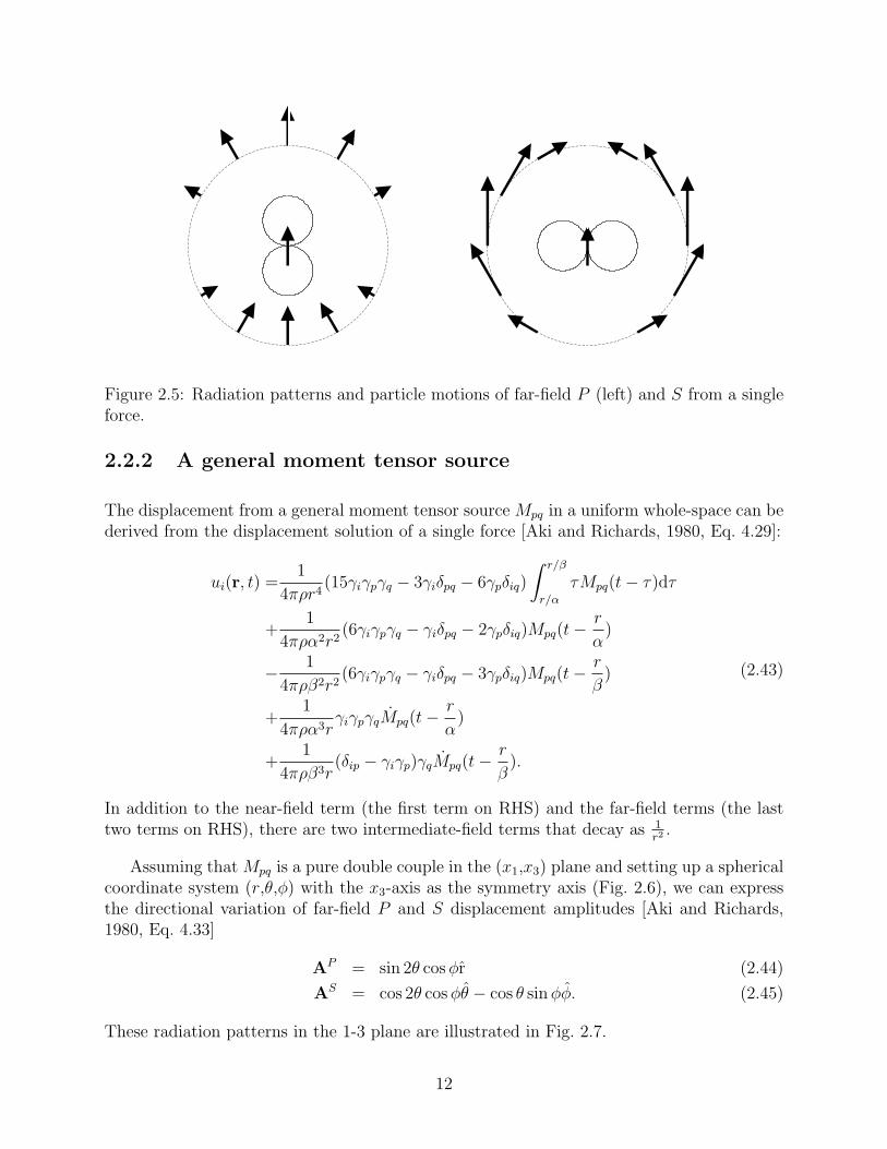
Figure 2.5: Radiation patterns and particle motions of far-field P (left) and S from a singleforce.
2.2.2 A general moment tensor source
The displacement from a general moment tensor source Mpq in a uniform whole-space can bederived from the displacement solution of a single force [Aki and Richards, 1980, Eq. 4.29]:
ui(r, t) =1
4πρr4(15γiγpγq − 3γiδpq − 6γpδiq)
∫ r/β
r/α
τMpq(t− τ)dτ
+1
4πρα2r2(6γiγpγq − γiδpq − 2γpδiq)Mpq(t−
r
α)
− 1
4πρβ2r2(6γiγpγq − γiδpq − 3γpδiq)Mpq(t−
r
β)
+1
4πρα3rγiγpγqMpq(t−
r
α)
+1
4πρβ3r(δip − γiγp)γqMpq(t−
r
β).
(2.43)
In addition to the near-field term (the first term on RHS) and the far-field terms (the lasttwo terms on RHS), there are two intermediate-field terms that decay as 1
r2 .
Assuming that Mpq is a pure double couple in the (x1,x3) plane and setting up a sphericalcoordinate system (r,θ,φ) with the x3-axis as the symmetry axis (Fig. 2.6), we can expressthe directional variation of far-field P and S displacement amplitudes [Aki and Richards,1980, Eq. 4.33]
AP = sin 2θ cosφr (2.44)
AS = cos 2θ cosφθ − cos θ sinφφ. (2.45)
These radiation patterns in the 1-3 plane are illustrated in Fig. 2.7.
12

θ
θ
r u
φ
φ
1
3
2
Figure 2.6: Displacement u produced by a double couple in the x1-x3 plane.
Figure 2.7: Radiation patterns and particle motions of far-field P (left) and S from a doublecouple.
2.2.3 Examples
Fig. 2.8 shows vertical acceleration recorded by TriNet station TAB from a nearby Mw 4.2earthquake near the San Andreas fault in California. The earthquake is 11 km deep andabout 3 km from the station. The obtained displacement using double integrations showsignificant near-field between the P and S phases and permanent displacement after the S.They are matched well by the whole-space solution prediction.
Near-field and permanent displacement have also been observed at regional distancesfrom large deep earthquakes such as the 1994 Bolivia deep earthquake (Fig. 2.9). Vidaleet al. [1995] reported an observation of the near-field of the Bolivia earthquake at stationsin southern California (7,500 km away) (Fig. 2.10).
13

−50
0
50
cm/s
**2
0 2 4 6
t (s)
−0.02
0.00
0.02
0.04
0.06
cm
Figure 2.8: The bottom trace is the vertical-component acceleration recorded by TriNetstation TAB from a nearby Mw 4.2 earthquake (3 km away and at a depth of 11 km). Thetop trace in black is the obtained displacement waveforms using double integration. Thered-colored trace is synthetic displacement using the whole-space solution (multiplied by 2to account for the free-surface effect).
2.3 Exercises
A sample Matlab program for computing displacement generated by a single force in a wholespace is given below:
%%%%%%%%%%%%%%%%%%%%%%%%%%%%%%%%%%%%%%%%%%%%%%%%%%%%%%%%%%%%%%%%%%
% computing displacements genenerated by a single force in a whole
% space.
%%%%%%%%%%%%%%%%%%%%%%%%%%%%%%%%%%%%%%%%%%%%%%%%%%%%%%%%%%%%%%%%%%
clear;
addpath /home/lupei/Src/sac_msc
% model parameters of the whole-space
vp = 6.3;
vs = 3.6;
% sampling rate
dt = 0.01;
% force vector
14

1
2
3
Dis
p. (c
m)
0 200 400 600
t (s)
T
R
Z
P
S
BANJO records of the 1994 Bolivia deep EQ
Figure 2.9: Black-colored traces are three-component displacement waveforms recorded atthe BANJO array from the 1994 Mw 8.3 Bolivia deep earthquake (from Zhu [2003]). Red-colored traces are synthetic displacements using the whole-space solution (multiplied by 2to account for the free-surface effect).
F = [0; 0; 1];
% receiver location
r = [3; 0; 10];
% compute the amplitudes of the nearfield and far-fields
dist = norm(r);
gamma = r/dist;
gammaDotF = gamma’*F;
AnearField = (3*gammaDotF*gamma-F)/(dist*dist*dist);
AfarP = gamma*(gammaDotF/(vp*vp*dist));
AfarS = (F-gammaDotF*gamma)/(vs*vs*dist);
% construct the time functions of the nearfield and far-fields
tp = dist/vp;
itp = round(tp/dt);
ts = dist/vs;
its = round(ts/dt);
nt = its + 100;
t = (0:nt-1)*dt;
15

Figure 2.10: Observation of near field at teleseismic distances from the 1994 Bolivia deepearthquake (from Vidale et al. [1995]).
nearField = zeros(3,nt);
farP = zeros(3,nt);
farS = zeros(3,nt);
nearField(:,itp:its) = AnearField*t(itp:its);
farP(:,itp) = AfarP/dt;
farS(:,its) = AfarS/dt;
disp = nearField + farP + farS;
subplot(4,1,1),plot(t,nearField(3,:))
subplot(4,1,2),plot(t,farP(3,:))
subplot(4,1,3),plot(t,farS(3,:))
subplot(4,1,4),plot(t,disp(3,:))
% save
compnm = ’xyz’;
hd = newhdr(nt,dt,0.);
for comp=1:3
wtSac([’nf.’ compnm(comp)], hd, nearField(comp,:));
wtSac([’fp.’ compnm(comp)], hd, farP(comp,:));
wtSac([’fs.’ compnm(comp)], hd, farS(comp,:));
end
16

%%%%%%%%%%%%%%%%%%%%%%%%%%%%%%%%%%%%%%%%%%%%%%%%%%%%%%%%%%%%%%%%%%
A low-pass filtered version of the waveforms is shown in Fig. 2.4.
1. Write a computer program to calculate displacement field produced by a moment tensorin a whole-space using (2.43). You should assume that the time history of the sourceis a step function.
2. TriNet station TAB recorded a magnitude 4.4 earthquake about 3 km away on Aug.20, 1998. According to waveform inversion, the event is located at a depth of 11 kmand its moment tensor elements are Mxx=-2.243, Mxy=-0.749, Mxz=-0.383, Myy=-0.226, Myz= 0.118, Mzz= 2.469, with a scale of 1022 dyne-cm, here the x-axis ispointing north, y east, and z downward. Use your program to compute and plot thevertical displacement waveform of each individual field and the total field. Comparethe synthetics with the observation obtained in Exe. 1.3 to find the appropriate Vp, Vs,and source rupture duration.
3. Use your program to model the displacement waveforms recorded at a BANJO sta-tion from the 1994 Bolivia deep earthquake (shown in Fig. 2.9). The station’s epi-central distance is 5.76◦and the azimuth is 181.53◦. The Harvard CMT solution isMxx=7.75, Mxy=-2.48, Mxz=-25.3, Myy=-0.16, Myz= 0.42, Mzz=-7.59, with ascale of 1027 dyne-cm, here the x-axis is pointing south, y east, and z up. The depthof the event after the Earth-flattening approximation is 682 km.
4. A strike-slip earthquake at 2 km depth ruptured a N-S oriented vertical plane of 6 kmlong and 2 km wide with a slip of 1 m. What is the moment magnitude of theearthquake (assumming that the rigidity is 30 GPa)? Modify your program to computeand plot horizontal permanent displacement field at the surface within 10 km from theepicenter. You need to divide the ruptured fault into small subfaults and sum up thecontribution from each point source.
17

Chapter 3
Multi-layered Media – GeneralizedRay Theory
3.1 Solution to wave equation in cylindrical coordinate
system
In cylindrical coordinates (r,θ,z) with the z-axis downward, the wave equation in the Laplacedomain is:
1
r
∂
∂r
(r∂φ
∂r
)+
1
r2
∂2φ
∂θ2+∂2φ
∂z2− s2
c2φ = 0. (3.1)
Using the variable separation method, the general solution from a point source at the originin a whole-space can be found as
φ(r, θ, z, s) =∑
n=0,±1,···
e−inθ
∫ ∞
0
An(k)Jn(kr)e−ν|z|dk, (3.2)
where
ν =
√k2 +
s2
c2, <ν > 0, (3.3)
and An is to be determined by initial conditions (i.e., the seismic source).
For example, the displacement field from an explosion source with a step source timefunction can be derived using (2.43) as
u(r, z, t) = ∇φ =M0
4πρc2
(H(t−R/c)
R2+H(t−R/c)
cR
)R, (3.4)
where R =√z2 + r2. So
φ(r, z, t) = − M0
4πρc2H(t−R/c)
R. (3.5)
18

By taking the Laplace transform and using the Somerfield integral,
φ(r, z, s) = − M0
4πρc21
s
e−sR/c
R= − M0
4πρc21
s
∫k
νJ0(kr)e
−ν|z|dk, (3.6)
i.e, the only non-zero term in (3.2) is n=0:
A0 = − M0
4πρc21
s
k
ν. (3.7)
3.2 A liquid whole-space
Let us consider an explosion source with a step source time function in a liquid whole-space.To get the time-domain solution for pressure φ(t), one needs to evaluate two integrals: onefor k (without − M0
4πρc2)
φ(s) =1
s
∫ ∞
0
k
νJ0(kr)e
−ν|z|dk, (3.8)
and another for the inverse Laplace transform of φ(s).
A technique call the Cagniard-de Hoop method can be used to evaluate the doubleintegrations at once. By variable substitution k = −isp and using
J0(−ispr) =i
π(K0(spr)−K0(−spr)) , (3.9)
(3.8) becomes
φ(s) = − i
π
∫ i∞
−i∞
p
ηK0(spr)e
−sη|z|dp =2
π=∫ i∞
0
p
ηK0(spr)e
−sη|z|dp, (3.10)
where
η =
√1
c2− p2. (3.11)
At large x,
Kn(x) =
√π
2xe−x
(1 +
4n2 − 1
8x+
(4n2 − 1)(4n2 − 9)
2(8x)2+ · · ·
). (3.12)
So, (3.10) becomes (only the first term is kept for simplicity)
φ(s) =
√2
πrs=∫ i∞
0
√p
ηe−s(pr+η|z|)dp. (3.13)
It looks very much like a Laplace transform when we introduce
t = pr + η|z|, (3.14)
19

βt=0 t=t0
p=1/cp=p0=sin /c*
β
Figure 3.1: Cagniard-de Hoop contour.
and require that t be real. The corresponding
p(t) =
rt
R2−√t20 − t2
R2|z|, t < t0,
rt
R2+ i
√t2 − t20R2
|z|, t > t0,
(3.15)
where R =√r2 + z2 and t0 = R
c. The above contour in the complex p-plane, called the
Cagniard-de Hoop contour, is show in Fig. 3.1. Because the integrant function is analyticalexcept along the real p axis for p > 1
c, the integration path [0, i∞] can be changed to along
the Cagniard-de Hoop contour and
J(t) = L−1
{=∫ i∞
0
√p
ηe−s(pr+η|z|)dp
}= =
{√p
η
dp
dt
}. (3.16)
So, the final solution for the pressure
φ(t) =1
π
√2
r
1√t∗ J(t). (3.17)
20

Since
dp
dt=
η√t20 − t2
, t < t0,
iη√t2 − t20
, t > t0,(3.18)
the largest contribution to J(t) occurs at time t = t0, which is the first arrival time. Using
the asymptotic behavior ofdp
dtnear t0, one can get
J(t) =
√r
2
H(t− t0)
R√t− t0
. (3.19)
So, the first-motion approximation of the solution
φ(t) =1
πR
1√t∗ H(t− t0)√
t− t0=H(t− t0)
R, (3.20)
which is the same as the exact solution.
3.3 Two liquid half-spaces
Figure 3.2: Two liquid half-spaces.
21

We now deal with two fluid half-spaces in contact at z = 0 (Fig. 3.2). The solution canbe found using the general solution and the boundary conditions of φ and 1
ρ∂φ∂z
continuous,
φ1(r, z, s) =
√2
πrs=∫ i∞
0
√p
η1
[e−s(pr+η1|z−z0|) +R12(p)e
−s(pr+η1|z+z0|)]dp, (3.21)
φ2(r, z, s) =
√2
πrs=∫ i∞
0
√p
η1
T12(p)e−s(pr+η1|z0|+η2z)dp, (3.22)
where
R12(p) =ρ2η1 − ρ1η2
ρ2η1 + ρ1η2
, (3.23)
T12(p) =2ρ2η1
ρ2η1 + ρ1η2
, (3.24)
are called the reflection and transmission coefficients of the interface, respectively. We rec-ognize that the first term of φ1 is the same as in the whole-space case. It represents theresponse of the direct wave. The Cagniard contour for the second term is defined by
t = pr + η1|z + z0|. (3.25)
Its first-motion arrival time t0 and p0 are found to be
t0 =R
c1, (3.26)
p0 =r
R
1
c1, (3.27)
where R =√r2 + (z + z0)2. They correspond to the arrival time and ray-parameter of
a geometrical ray that is reflected from the interface. So, the second term represents theresponse of the reflected wave.
If c2 > c1, the reflection coefficient can become complex even when p < p0. This meansthat J(t) can be non-zero before the arrival time t0 of the geometrical reflection ray (Fig. 3.3).This non-geometrical arrival time is
tc =r
c2+
√1
c21− 1
c22|z + z0|, (3.28)
where is the head-wave arrival time.
Fig. 3.4 shows vertical displacement waveforms in such a two liquid half-space model
22

β
t=0 t=t0
1/c1p=p0=sin /c1
*β1/c2
Figure 3.3: Cagniard contour for reflection ray in two liquid half-spaces.
3.4 A sandwiched liquid layer between two liquid half-
spaces
If we add a layer of fluid of thickness d between the two half-spaces, the pressure solution inthe top liquid is
φ1(r, z, s) =
√2
πrs=∫ i∞
0
√p
η1
[e−s(pr+η1|z−z0|) + A(p)e−s(pr+η1|z+z0|)
]dp, (3.29)
where
A(p) =R12 +R23e
−2sη2d
1 +R12R23e−2sη2d. (3.30)
We can use its Taylor expansion
A(p) = R12 +∞∑
n=1
(−1)n+1Rn−112 Rn
23(1−R212)e
−2nsη2d. (3.31)
So the pressure can be writtern as
φ1 = φdirect + φreflected +∞∑
n=1
φn, (3.32)
23

0
10
20
30
40
50
60
70
80
90
100d
(km
)
1 2 3 4 5 6 7 8
t-d/7.5 (s)
Pn PmP
Figure 3.4: Vertical displacements produced by an explosion in a two liquid half-space model,located 5 km above the contact interface. The P velocity in the top half-space is 5 km/s,and 7.5 km/s in the bottom half-space.
24

where
φn =
√2
πrs=∫ i∞
0
T12(−R12)n−1Rn
23T21
√p
η1
e−s(pr+η1|z+z0|+2nη2d)dp. (3.33)
It can be recognized that φn corresponds to a geometrical ray with n-time internal reflectionsin the liquid layer.
(3.32) means that the full response can be constructed by adding up responses of allpossible “rays” from the source to the receiver. The technique is called generalized raytheory. It was first introduced by Spencer [1960].
3.5 Double-couple sources in elastic media
For isotropic elastic media, the displacement field u satisfies a second-order differential equa-tion:
∂2u
∂t2=
1
α2∇∇ · u− 1
β2∇× (∇× u). (3.34)
By using the Helmholtz representation of a vector
u = ∇φ+∇× χz− 1
sp∇× (∇× ψz), (3.35)
we obtain three wave equations:
∇2φ =1
α2
∂2φ
∂t2, (3.36)
∇2ψ =1
β2
∂2ψ
∂t2, (3.37)
∇2χ =1
β2
∂2χ
∂t2, (3.38)
where φ is called the P -wave potential, ψ SV potential, and χ SH potential.
For a double-couple source, the non-zero terms in the general solution (3.2) of thesepotentials are limited to n ≤ 2:
φ =M0
4πρ
2∑n=0
An(θ, λ, δ)2
π=∫ i∞
0
Cnp
ηα
Kn(spr)e−sηα|z|dp, (3.39)
ψ =M0
4πρ
2∑n=0
An(θ, λ, δ)2
π=∫ i∞
0
SVnp
ηβ
Kn(spr)e−sηβ |z|dp, (3.40)
χ =M0
4πρ
2∑n=1
1
n
∂
∂θAn(θ, λ, δ)
2
π=∫ i∞
0
SHnp
ηβ
Kn(spr)e−sηβ |z|dp. (3.41)
25
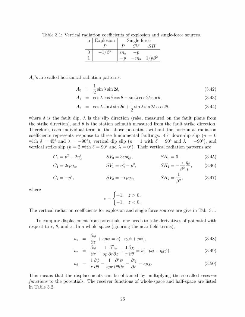
Table 3.1: Vertical radiation coefficients of explosion and single-force sources.n Explosion Single force
P P SV SH0 −1/β2 εηα −p1 −p −εηβ 1/pβ2
An’s are called horizontal radiation patterns:
A0 =1
2sinλ sin 2δ, (3.42)
A1 = cosλ cos δ cos θ − sinλ cos 2δ sin θ, (3.43)
A2 = cosλ sin δ sin 2θ +1
2sinλ sin 2δ cos 2θ, (3.44)
where δ is the fault dip, λ is the slip direction (rake, measured on the fault plane fromthe strike direction), and θ is the station azimuth measured from the fault strike direction.Therefore, each individual term in the above potentials without the horizontal radiationcoefficients represents response to three fundamental faultings: 45◦ down-dip slip (n = 0with δ = 45◦ and λ = −90◦), vertical dip slip (n = 1 with δ = 90◦ and λ = −90◦), andvertical strike slip (n = 2 with δ = 90◦ and λ = 0◦). Their vertical radiation patterns are
C0 = p2 − 2η2α SV0 = 3εpηβ, SH0 = 0, (3.45)
C1 = 2εpηα, SV1 = η2β − p2, SH1 = − ε
β2
ηβ
p, (3.46)
C2 = −p2, SV2 = −εpηβ, SH2 =1
β2, (3.47)
where
ε =
{+1, z > 0,
−1, z < 0.
The vertical radiation coefficients for explosion and single force sources are give in Tab. 3.1.
To compute displacement from potentials, one needs to take derivatives of potential withrespect to r, θ, and z. In a whole-space (ignoring the near-field terms),
uz =∂φ
∂z+ spψ = s(−ηαφ+ pψ), (3.48)
ur =∂φ
∂r− 1
sp
∂2ψ
∂r∂z+
1
r
∂χ
∂θ= s(−pφ− ηβψ), (3.49)
uθ =1
r
∂φ
∂θ− 1
spr
∂2ψ
∂θ∂z− ∂χ
∂r= spχ. (3.50)
This means that the displacements can be obtained by multiplying the so-called receiverfunctions to the potentials. The receiver functions of whole-space and half-space are listedin Table 3.2.
26

Table 3.2: Whole-space and half-space receiver functions.Whole-space Half-spaceP SV SH P SV SH
uz −ηα p −2ηα(η2β − p2)/D 4pηαηβ/D
ur −p -ηβ −4pηαηβ/D −2ηβ(η2β − p2)/D
uθ p 2p
D =((η2
β − p2)2 + 4p2ηαηβ
)β2 is called the Rayleigh denominator.
The Rayleigh denominator D in the half-space receiver functions is interesting. It has aroot at p ≈ 1.1β−1 on the real p axis (called the Rayleigh pole). When the source is shallow,the Cagniard contour is close to the real p axis so that J(t) has large amplitudes at timeswhen the contour is close to the Rayleigh pole. It gives large-amplitude Rayleigh surfacewaves on the z and r components, with an apparent velocity of 0.9β. An example is shownin Fig. 3.5
The generalized reflection and transmission coefficients across solid-solid and solid-liquidinterfaces can be found in Helmberger [1968].
27

0
10
20
30
40
50
60
70
80
90
100d
(km
)
0 1 2 3 4 5 6 7 8 9 10 11 12 13 14
t−d/6.3 (s)
sP S
Figure 3.5: Vertical displacements from a strike-slip fault at 5 km depth in a uniform half-space (Vp 6.3 km/s, Vs 3.6 km/s, and ρ 2.7 g/cm3).
28

3.6 Exercises
A sample Matlab program for computing the Cagniard-de Hoop coutour and pressure pro-duced by an explosion in a liquid wholespace is given below:
%%%%%%%%%%%%%%%%%%%%%%%%%%%%%%%%%%%%%%%%%%%%%%%%%%%%%%%%%%%%%%%%%
% computing pressure generated by an explosion in fluid using
% the Cagniard-de Hoop method
%%%%%%%%%%%%%%%%%%%%%%%%%%%%%%%%%%%%%%%%%%%%%%%%%%%%%%%%%%%%%%%%%
clear
addpath /home/lupei/Src/sac_msc
% model: a fluid whole space
c=5.0; rho=1.0;
% source depth
h=5;
% receiver location
r=10;
nx = length(r);
z=h;
% time window
dt = 0.01;
n = 700;
nbefore = 100;
scale = -1/(4*pi*rho*c^2);
a = 2*sqrt((0:n-1)/dt); % 2*sqrt(t)
eps = 1.e-8; % small positive imaginary part
for ix=1:nx
R = sqrt(r(ix)*r(ix)+h^2);
t0 = R/c;
t = t0 + dt*(-nbefore:n-nbefore-1)’ + 0.5*dt;
p = (r(ix)/R^2)*t - (z/R^2)*sign(t0-t).*sqrt(t0^2-t.^2)+eps*i;
eta = sqrt(1/c^2-p.^2);
% j(t)
dpdt = sign(t0-t).*eta./sqrt(t0^2-t.^2);
jt = imag((sqrt(p)./eta).*dpdt);
% convolve with sqrt(t) and take a derviative
phi = (scale*sqrt(2./r(ix))/pi)*diff(conv(a,jt));
hd = newhdr(n-2,dt,t(2));
hd(51) = r(ix);
wtSac([’phi.’ num2str(r(ix))],hd,phi);
end
% plotting
29

subplot(3,1,1);
plot(p,’+’);
subplot(3,1,2);
plot(t,jt);
subplot(3,1,3);
plot(t(2:n-1),phi(1:n-2));
%%%%%%%%%%%%%%%%%%%%%%%%%%%%%%%%%%%%%%%%%%%%%%%%%%%%%%%%%%%%%%%%%
1. Write a Matlab program to plot vertical radiation patterns (3.45)-(3.47) as a functionof take-off angle.
2. Modify the sample Matlab code above to compute vertical displacements of reflectedwaves from an explosion source in two liquid half-spaces. Note that the whole spacereceiver function for uz is −sηα. The source and stations are 5 km above the interfacein the top half-space with a P velocity of 5 km/s. The P velocity in the bottom halfspace is 7.5 km/s. Plot waveform profile from 10 to 100 km in epicentral distances.
3. Use the GRT program aser to repeat the above computation and compare the results.Note that the GRT outputs are impulse responses and need to be integrated to get thestep responses in order to compare with the Matlab results. A sample GRT input isgiven below:
n # debug
n # Q individual rays
3 # number of terms for the Bessel function expansion
0.01 800 # dt and nt
2 # sample rate of the Cagniard contour, 0=FM
3 # number of layers in the model
5.0 6.3 3.6 2.786 1000 500 # the 1st layer
5.0 6.3 3.6 2.786 1000 500 # the 2nd layer
0.0 8.0 4.5 3.000 1000 500 # the bottom halfspace
2 1 # The source type (0=EX, 1=SF; 2=DC) and source layer (at its top)
rays.file # The name of the ray file
4 # number of distance rangesi, followed by distance t0 name (2f10.3,1x,a80)
1.000 0.500 grt/01.grn.
5.000 1.000 grt/05.grn.
10.000 1.500 grt/10.grn.
50.000 7.500 grt/50.grn.
#
# The ray file looks like this:
1 # number of rays
p 2 1p 1p 0.00
# wave type (p/s/t), number of seg., ray seg specification, ..., shift
30

Chapter 4
Multi-layered Media –Frequency-Wavenumber IntegrationMethod
4.1 Displacement-stress vector in a source-free homo-
geneous medium
We set up a cylindrical coordinate system (er, eθ, ez), with ez pointing upward. The displace-ment in a vertically heterogeneous medium can be expanded in terms of three orthogonalvectors [e.g. Takeuchi and Saito, 1972]:
u(r, θ, z, t) =1
2π
∑m=0,±1,···
∫e−i ω t dω
∫ ∞
0
k dk(UzR
km + UrS
km + UθT
km
), (4.1)
Rkm,S
km,T
km are called the surface vector harmonics:
Rm = −Ymz, (4.2)
Sm =1
k∇Ym =
1
k
∂Ym
∂rr +
1
kr
∂Ym
∂θθ, (4.3)
Tm = Sm × z =1
kr
∂Ym
∂θr− 1
k
∂Ym
∂rθ, (4.4)
whereYm(r, θ) = Jm(kr)eimθ. (4.5)
Similar expansion can be done to the traction on the horizontal plane
σ(r, θ, z, t) =1
2π
∑m=0,±1,···
∫e−i ω t dω
∫ ∞
0
k2 dk(TzR
km + TrS
km + TθT
km
). (4.6)
31

Note that a factor k is drawn from the Tz, Tr and Tθ to simplify the later derived matrices.Eq. (4.1) and (4.6) separate the z-variation of the displacement and stress from the (r, θ)variations. Under this expansion, the second-order differential equation of motion
(λ+ 2µ)∇ (∇ · u)− µ∇×∇× u + ρω2u = 0, (4.7)
is reduced to a set of first-order ordinary differential equations
d
dz
Ur
Uz
Tz
Tr
Uθ
Tθ
= k
0 −1 0 1µ
0 0
1− 2 ξ 0 ξµ
0 0 0
0 −ρ(
ωk
)20 1 0 0
4µ ξ1 − ρ(
ωk
)20 2 ξ − 1 0 0 0
0 0 0 0 0 1µ
0 0 0 0 µ− ρ(
ωk
)20
Ur
Uz
Tz
Tr
Uθ
Tθ
, (4.8)
or, in the vector-matrix form:db(z)
dz= Mb(z). (4.9)
Here, ρ is the density; ξ = µ/(λ+ 2µ); ξ1 = 1− ξ; λ, µ are the Lame constants. The vectorb is often called the displacement-stress vector. Note that M can be partitioned into a 4×4submatrix describing the motion in the (z, r) plane and a 2×2 submatrix for the motion inthe θ-direction. They are often referred to as the P -SV system and the SH system. We willconcentrate on the P -SV problem. The corresponding solution for the SH problem can befind in Appendix A.
For a homogeneous medium, M is constant. In this case, the general solution of (4.9) is
b(z) = ez M b0. (4.10)
To calculate the matrix exponential, we use the Jordan decomposition of M [e.g. Turnbulland Aitken, 1952, Gantmatcher, 1960]:
M = EJE−1, (4.11)
where E is a similarity matrix and J is the Jordan canonical form of M. Using (4.11) andthe definition of matrix exponential, we have
ez M = E ez J E−1. (4.12)
From (4.10) and (4.12), the displacement-stress at any z can be expressed as
b(z) = EΛ(z)w, (4.13)
whereΛ(z) = ez J, (4.14)
and w is a constant vector that is to be determined by boundary conditions.
32
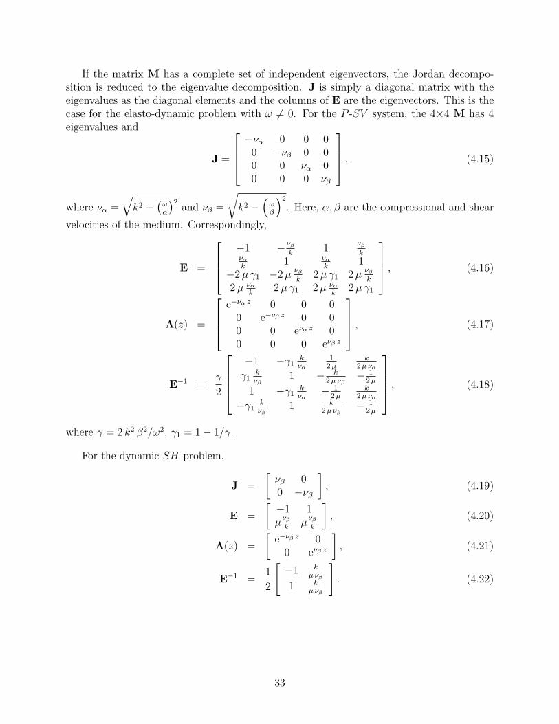
If the matrix M has a complete set of independent eigenvectors, the Jordan decompo-sition is reduced to the eigenvalue decomposition. J is simply a diagonal matrix with theeigenvalues as the diagonal elements and the columns of E are the eigenvectors. This is thecase for the elasto-dynamic problem with ω 6= 0. For the P -SV system, the 4×4 M has 4eigenvalues and
J =
−να 0 0 00 −νβ 0 00 0 να 00 0 0 νβ
, (4.15)
where να =√k2 −
(ωα
)2and νβ =
√k2 −
(ωβ
)2
. Here, α, β are the compressional and shear
velocities of the medium. Correspondingly,
E =
−1 −νβ
k1
νβ
kνα
k1 να
k1
−2µ γ1 −2µνβ
k2µ γ1 2µ
νβ
k
2µ να
k2µ γ1 2µ να
k2µ γ1
, (4.16)
Λ(z) =
e−να z 0 0 0
0 e−νβ z 0 00 0 eνα z 00 0 0 eνβ z
, (4.17)
E−1 =γ
2
−1 −γ1
kνα
12 µ
k2 µ να
γ1kνβ
1 − k2 µ νβ
− 12 µ
1 −γ1kνα
− 12 µ
k2 µ να
−γ1kνβ
1 k2 µ νβ
− 12 µ
, (4.18)
where γ = 2 k2 β2/ω2, γ1 = 1− 1/γ.
For the dynamic SH problem,
J =
[νβ 00 −νβ
], (4.19)
E =
[−1 1µ
νβ
kµ
νβ
k
], (4.20)
Λ(z) =
[e−νβ z 0
0 eνβ z
], (4.21)
E−1 =1
2
[−1 k
µ νβ
1 kµ νβ
]. (4.22)
33

::
::
EN+1
0
m+1
1
m-1
N
mz=0
z=h
a m+1
a m
a 1
Figure 4.1: A layered half-space consists of N layers over a half-space at the bottom. Thesource is located at a depth of h between layer m and m+1 with identical elastic properties.
4.2 Surface displacement of layered half-space from an
embedded point source
The general description of model is shown in Figure 4.1. It consists of a stack of layers ontop of half space, with source embedded somewhere in the middle. The solution to the waveequation within each layer is represented by the wave-vector wn. The boundary conditionsare:
1. Continuity of displacement and stress across all interfaces except at the source interface.
2. Vanishing of up-going waves in the half space.
3. Vanishing of stress at the free surface.
34

From (4.13) the stress-displacement vectors at top and bottom of layer n are:
bn−1 = EnΛn(zn−1)wn, (4.23)
bn = EnΛn(zn)wn, (4.24)
which lets us to “propagate” the stress-displacement vector from the top to the bottom:
bn = anbn−1, (4.25)
wherean = EnΛn(zn − zn−1)E
−1n = EnΛn(dn)E−1
n . (4.26)
The a matrix is often called Thompson-Haskell propagation matrix [Haskell, 1964, Wangand Herrmann, 1980]:
For the P -SV system
an = γ
Cα − γ1Cβ γ1 Yα −Xβ
Cβ−Cα
2 µ
Xβ−Yα
2 µ
γ1 Yβ −Xα Cβ − γ1CαXα−Yβ
2 µ
Cα−Cβ
2 µ
2µ γ1 (Cα − Cβ) 2µ (γ12 Yα −Xβ) Cβ − γ1Cα Xβ − γ1 Yα
2µ (γ12 Yβ −Xα) 2µ γ1 (Cβ − Cα) Xα − γ1 Yβ Cα − γ1Cβ
, (4.27)
where Cα = cosh(να d), Xα = να sinh(να d)/k, and Yα = k sinh(να d)/να, and similarly forCβ, Xβ, and Yβ. d = zn−1 − zn is the thickness of the layer. Our an is different fromthe original one given by Haskell [1964] for the traction related terms. This stems fromthe difference of our definition of the displacement-stress vector from the Haskell’s in whichhe multiplied the traction by ω2. As shown later, the Haskell’s definition introduces theapparent ω-dependence of source terms and causes difficulty to unify the elasto-dynamicsolution and the elasto-static solution.
For the SH problem, the Thomson-Haskell propagator matrix is
a =
[Cβ −Yβ
µ
−µXβ Cβ
]. (4.28)
At the interface where the source is located, b is discontinuous due to the presence ofthe source:
b−m = b+
m − s. (4.29)
Since b is continuous at all other interfaces, we can connect the wave-vector in half spacewith the stress-displacement vector at the surface
ΛN+1(zN)wN+1 = Xb−m = X (b+
m − s) = Rb0 −Xs, (4.30)
where
X = E−1N+1aN · · · am+1, (4.31)
R = E−1N+1aN · · · a1. (4.32)
35

The stress-free surface boundary condition means that for b0:
Tz = Tr = Tθ = 0. (4.33)
In the bottom half-space, the components of wN+1 associated with up-going waves e−να,βz
should vanish:wN+1(1) = wN+1(2) = wN+1(5) = 0. (4.34)
We then get:R11 R12 0R21 R22 00 0 R55
Ur
Uz
Uθ
−X11 X12 X13 X14 0 0X21 X22 X23 X24 0 00 0 0 0 X55 X56
s =
000
. (4.35)
Solving above linear equations, we can obtain the displacement at the surface:(Ur
Uz
)=
1
FR
(R22 −R12
−R21 R11
)(X1isi
X2isi
), (4.36)
Uθ =X5isi
FL
, (4.37)
where
FR = R11R22 −R21R12, (4.38)
FL = R55, (4.39)
are often called Rayleigh denominator and Love denominator.
As an example, consider a half space,
R = E−1, (4.40)
The Rayleigh denominator
FR = R11R22 −R21R12 =1
k2
((1− γ)2k2 − γ2νανβ
), (4.41)
Figure 4.2 plots FR as a function of k.
For a layer over half space,R = E−1
2 a1, (4.42)
The Love denominator:
FL = R55 = −1
2
(cosh νβ1d−
ρ1νβ1β21
ρ2νβ2β22
sinh νβ1d
), (4.43)
which is shown in Figure 4.3.
36
0.1 0.2 0.3 0.4 0.5
5
10
15
20
Kα KβWavenumber (1/km)
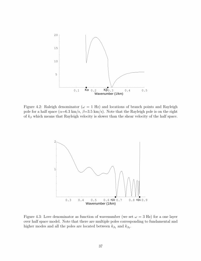
Figure 4.2: Raleigh denominator (ω = 1 Hz) and locations of branch points and Rayleighpole for a half space (α=6.3 km/s, β=3.5 km/s). Note that the Rayleigh pole is on the rightof kβ which means that Rayleigh velocity is slower than the shear velocity of the half space.
0.3 0.4 0.5 0.6 0.7 0.8 0.9
1
2
Wavenumber (1/km)Kβ2 Kβ1
Figure 4.3: Love denominator as function of wavenumber (we set ω = 3 Hz) for a one layerover half space model. Note that there are multiple poles corresponding to fundamental andhigher modes and all the poles are located between kβ1 and kβ2 .
37

4.3 Source terms and horizontal radiation pattern
The displacement-stress discontinuities to represent the source can be found by expandingthe solution of the whole-space problem with the cylindrical spherical harmonics (4.1 and4.6) [Haskell, 1953, Takeuchi and Saito, 1972]. Takeuchi and Saito [1972] have listed thedisplacement-stress discontinuities produced by various sources. Since our definition of sis slightly different from theirs, we will give below the non-zero terms for several types ofsources often encountered in seismology.
4.3.1 Explosion source
Only m = 0 term exists for the isotropic source
s0 = (0, ξ/µ, 0, 2ξ, 0, 0)T . (4.44)
4.3.2 Single force
None-zero terms exist for m = 0, ±1. We use the symmetry between m = −1 and m = 1terms and factor out the common source geometry independent term. This reduces thenumber of source vectors s from 3 to 2:
s0 =1
k(0, 0, −1, 0, 0, 0)T , (4.45)
s1 =1
k(0, 0, 0, −1, 0, 1)T . (4.46)
They will produce five components of ground displacement, u0z, u
0r, u
1z, u
1r, u
1θ (u0
θ is alwayszero). The actual displacement is obtained by adding the force orientation when summingover azimuthal modes m. By re-arranging terms, the summation can be expressed as
uz = cosφ cos δ u1z − sin δ u0
z, (4.47)
ur = cosφ cos δ u1r − sin δ u0
r, (4.48)
uθ = − sinφ cos δ u1θ, (4.49)
where δ is the dip angle of the force, measured from the horizontal plane; φ is the azimuthof the station, measured clockwise from the direction of the force. It can be seen that u0
is produced by an unit vertical force (upward) and u1 is produced by a horizontal force ofmagnitude
√2 at azimuth 45◦ CCW from the force direction.
38

4.3.3 Double-couple without torque
Similar to the single force, the five none-zero source vectors (m = 0, ±1, ±2) can be reducedto three:
s0 = (0, 2 ξ/µ, 0, 4 ξ − 3, 0, 0)T , (4.50)
s1 = (1/µ, 0, 0, 0, −1/µ, 0)T , (4.51)
s2 = (0, 0, 0, 1, 0, −1)T . (4.52)
The displacement for arbitrary double-couple is
uz =1
2sin 2 δ sinλu0
z
− (sinφ cos 2δ sinλ− cosφ cos δ cosλ)u1z
− (sin 2φ sin δ cosλ+1
2cos 2φ sin 2δ sinλ)u2
z, (4.53)
ur =1
2sin 2 δ sinλu0
r
− (sinφ cos 2δ sinλ− cosφ cos δ cosλ)u1r
− (sin 2φ sin δ cosλ+1
2cos 2φ sin 2δ sinλ)u2
r, (4.54)
uθ = −(sinφ cos δ cosλ+ cosφ cos 2δ sinλ)u1θ
+ (1
2sin 2φ sin 2δ sinλ− cos 2φ sin δ cosλ)u2
θ, (4.55)
where δ is the dip angle of the fault plane; λ is the slip direction measured counterclockwisefrom the strike of the fault; φ is the azimuth of the station, measured clockwise from thestrike of the fault. The above coefficients are often called the horizontal radiation patternsand were given by different authors [e.g. Aki and Richards, 1980, Wang and Herrmann, 1980,Helmberger, 1983]. The results show that u0 is produced by a 45◦ down-dip slip (magnitude-2) at azimuth 45◦ from the fault strike, u1 is produced by a vertical dip slip (magnitude-√
2) at azimuth 45◦, and u2 is produced by a vertical strike slip (magnitude -√
2) at azimuth22.5◦.
4.4 Frequency-wavenumber integration
Calculation of Green’s function involves following double integration:∫ ∞
0
eiωtdω
∫ ∞
0
U(ω, k)Jn(kr) dk, (4.56)
which can be done in different ways (GRT, slowness method, etc). The frequency-wavenumber(F-K) integration method that we are going to discuss below does the k-integration first bysome numerical integration scheme. The ω-integration is then easily implemented by theinverse fast Fourier transform (IFFT).
39

-
6
tkα tkβ d dpoles Re{k}
Im{k}
Figure 4.4: Location of branch points and poles in complex k-plane.
4.4.1 Wavenumber integration
The k-integration over the real k-axis from 0 to ∞ is complicated by several issues. First,the branch points kα, kβ, and also the Rayleigh poles and Love poles, are all located onthe real axis (Figure 4.4). This makes the numerical computation of U(ω, k) very unstable.Fortunately for anelastic medium, the velocities are complex and frequency-dependent:
v = vr(1 +1
πQlog f +
i
2Q), (4.57)
where vr is the reference velocity at 1 Hz. Since
kα =ω
α, kβ =
ω
β, (4.58)
all the branch points and poles are moved below the real k axis. As shown in Figure 4.5,introducing attenuation in the velocity model helps to smooth the kernel and stabilize thecalculation.
Another way to stabilize the computation of U(ω, k) along real k-axis is to introduce asmall negative imaginary part in ω, while will also move branch points below the real k axis.Instead of calculating U(ω, k), we now calculate U(ω − σi, k). Because
IFFT [f(ω − σi)] = e−σtf(t) +∑n6=0
f(t+ nT )e−σ(t+nT ), (4.59)
where T = 2πdω
, this small imaginary part helps to damp the time sequence and reducewrap-around (time aliasing).
Integration using trapezoidal rule
A simple integration scheme is to use trapezoidal rule:∫ k1+dk
k1
g(k) dk =dk
2(g(k1) + g(k1 + dk)), (4.60)
40

0.3 0.4 0.5 0.6 0.7 0.8 0.9 1.0
Wavenumber (1/Km)
Q = ∞, σ=0
Q = 500, σ=0
Q = 500, σ=0.01
k k k kα α2 1 β 2 β1 Rayleigh pole
Figure 4.5: Vertical displacement kernel as function of k for different Qβ and σ value (weset ω = 0.47 Hz). The velocity model is a one-layer over half-space, with α1 = 6.3, β1 =3.5, α2 = 8.1, β2 = 4.5.
where g(k) = U(k)Jn(kr). So the integration from k = 0 to kmax can be approximated by(assuming g(0) = g(kmax) = 0, which is usually the case):∫ kmax
0
g(k) dk = dk(g1 + g2 + · · ·+ gn). (4.61)
Usually the integrand g(k) is highly oscillatory, especially at large r (Figure 4.6). Gener-ally the trapezoidal rule is not a good scheme for this kind of integration. However, from aphysical point of view, replacing continuous k-integral with summation of discrete horizon-tal wavenumbers is equivalent to summing all contributions from infinite number of pointsources uniformly distributed in horizontal plane [Bouchon, 1981], with separation distance:
L =2π
dk, (4.62)
(Figure 4.7). So, as long as this separation satisfies:
L > 2r, (4.63)√(L− r)2 + h2 > vmaxt, (4.64)
the wavefield obtained at (r, t) will not be disturbed by the closest neighbor source.
41

0.2 0.4 0.6 0.8 1.0
k (1/km)
Figure 4.6: F-K integrand U(ω, k)J0(kx) at distance ranges of 100 km (above) and 1000 km(below).
����������
LL
LL
LL
LL
LLt
d d t d dL = 2πdk
h
r
√(L− r)2 + h2
Figure 4.7: Discrete summation in wavenumber is equivalent to summing infinite number ofpoint sources (open circles) uniformly distributed in r direction.
42

2 4 6 8 10
0.5
1
1.5
x
Figure 4.8: Bessel function J0(x) (solid line) and its first term of asymptotic expansion√2
πxcos(x− π
4) (dashed line).
Filon scheme
Another method often used for integrating oscillatory functions is the Filon scheme [e.g.Saikia, 1994]. It tries to separate the kernel U(k) from the more oscillatory Bessel functionJn(kr) through integration by parts.
First we express Bessel function in terms of Hankel functions:
Jn(kr) =H
(1)n (kr) +H
(2)n (kr)
2. (4.65)
As kr � 1, we have:
H(1)n ∼
√2
πkreikr, (4.66)
H(2)n ∼
√2
πkre−ikr. (4.67)
Dropping the H(1)n term which represents inward propagating waves, and integrating by
parts: ∫ k1+dk
k1
U(k)e−ikr dk = − 1
ir(Ue−ikr)|k1+dk
k1+
1
ir
∫ k1+dk
k1
U ′e−ikr dk. (4.68)
Assuming U(k) is linear between k1 and k1 + dk, RHS can be written as:
− 1
ir(g(k1 + dk)− g(k1)) +
U(k1 + dk)− U(k1)
irdk
∫ k1+dk
k1
e−ikr dk
=− 1
ir(g(k1 + dk)− g(k1)) +
U(k1 + dk)− U(k1)
r2dk(e−ir(k1+dk) − e−irk1),
(4.69)
43

finally, we have: ∫ k1+dk
k1
U(k)e−ikr dk = dk(c g(k1) + c g(k1 + dk)), (4.70)
where
c =1− cos ε+ i(sin ε− ε)
ε2, (4.71)
ε = rdk. (4.72)
So, the integration can be approximated by:∫ kmax
0
g(k) dk = 21− cos ε
ε2dk(g1 + g2 + · · ·+ gn). (4.73)
Note that above formula differs from (4.61) only by a coefficient. So the two schemes shouldgive same waveform shapes with different amplitudes. Numerical test shows that the Filonscheme gives poor amplitude prediction. The reason is that the assumption it made aboutkernel’s linear behavior between any two sampling points is not proper in our case.
4.4.2 Compound matrix
Haskell propagator matrix elements contain exponential function like e±νd. Multiplicationof propagator matrices of several layers usually causes severe loss of significant digits andleads to large numerical errors. A solution is to use the so-called compound matrix insteadof the Haskell matrix itself. The compound matrix of A is formed by its subdeterminants:
A|ijkl = AikAjl − AilAjk. (4.74)
By factoring R into two partsR = XZ, (4.75)
whereZ = am . . . a1, (4.76)
is the propagator matrix from the surface to above the source, the displacement kernels inEq. (4.36) can be expressed as:(
Ur
Uz
)=
1
R|1212
(siX|12ij Zj2
−siX|12ij Zj1
), (4.77)
where
X|12ij = (E−1N+1)|
12mnaN |mn
op . . . am+1|stij , (4.78)
R|1212 = (E−1N+1)|
12mnaN |mn
op . . . a1|st12. (4.79)
Note that the 4×4 matrix X|12ij can also be viewed as a 1×6 row vector
g = (X|1212,X|1213,X|1214,X|1223,X|1224,X|1234), (4.80)
which is to be propagated upward by the 6×6 compound matrix, see Wang and Herrmann[1980] for details.
44
4.4.3 Other boundary conditions
If the top interface is not a free surface but the bottom of an elastic half-space, the stress-freeboundary condition is replaced by the vanishing of down-going waves in the top half-space.The equation takes the same form of Eq. (4.30) except the matrix R is multiplied from theright by matrix E0 of the top half-space.
If the bottom interface is a free boundary, the LHS of Eq. (4.30) is replaced by thedisplacement-stress vector at the bottom with rows 3 and 4 vanished. By multiplying bothsides by
H =
0 0 1 00 0 0 11 0 0 00 1 0 0
, (4.81)
we swap rows 1–2 with 3–4 thus obtain the same format solution of Eq. (4.36), except thatE−1
N is replaced by H in L and R. Similar technique can be used to handle rigid bottomboundary condition by using an unit matrix for H, see Herrmann [2007].
4.4.4 Buried receivers
For obtaining displacement kernels for buried receivers beneath the surface but above thesource level, one might attempt to obtain the surface displacement vector first and then usethe Haskell matrix to propagate it down to the receiver depth:
Ur
Uz
Tz
Tr
=Y
R|1212
siX|12ij Zj2
−siX|12ij Zj1
00
, (4.82)
where Y is the propagator matrix from the surface to the receiver. This approach is, however,not numerically stable at high frequencies due to the exponential functions in the Haskellmatrix. Herrmann [2007] used the compound matrix by replacing the Z matrix above with
Z = VY, (4.83)
where V is the propagator matrix from the receiver to the source. The displacement-stressvector at the buried receiver becomes
Ur
Uz
Tz
Tr
=1
R|1212
siX|12ij VjkY|1k
12
siX|12ij VjkY|2k12
siX|12ij VjkY|3k12
siX|12ij VjkY|4k12
. (4.84)
If the receiver is below the source, one can flip the model to carry out the same com-putations and correct the vertical displacement polarity when done. In the process, sourcevectors s0 of single force and s1 of double couple need to be reversed.
45

4.4.5 Partitioning of up-going and down-going wavefields
Partitioning of total wavefield into up-going and down-going wavefields is done by separatingthe source displacement-stress jump vector s into the up-going and down-going parts:
s = s+ + s− = (D+ + D−)s. (4.85)
For the P -SV system,
D+ = E
1 0 0 00 1 0 00 0 0 00 0 0 0
E−1
=1
2
1 γ
(γ1k
να
− νβ
k
)0
γ
2µ
(νβ
k− k
να
)γ
(γ1k
νβ
− να
k
)1
γ
2µ
(να
k− k
νβ
)0
0 2µγ
(γ2
1
k
να
− νβ
k
)1 γ
(νβ
k− γ1
k
να
)2µγ
(γ2
1
k
νβ
− να
k
)0 γ
(να
k− γ1
k
νβ
)1
,
(4.86)
and for the SH system,
D+ =1
2
1k
µνβµνβ
k1
. (4.87)
4.4.6 Some practical aspects in the F-K integration
I have written a Fortran code to implement the propagator matrix algorithm to compute thedisplacement kernels. This code closely follows the notations of Zhu and Rivera [2002]. Thestructure of the Fortran program to calculate F-K integration can be illustrated as following:
for frequency = ωmin to ωmax step dωfor wavenumber = kmin to kmax step dk
for layer = bottom to topcalculating propagation matrix
end of layer loopcalculating kernel U(k, ω)summing J(kx)U(k, ω)
end of wavenumber loopend of frequency loop
46

inverse Fourier transformation
There are essentially three loops in the computation, i.e., layer-propagation, k-loop, andω-loop. For each k and ω, the code starts at the bottom half space, initializing the g withthe (E−1
N+1)|12ij . Then it propagates this 1×6 vector upward using the compound matrix ofeach layer. When crossing the source interface, it initializes the 1×4 vector zj = siX|12ij
and then propagates it upward using the Haskell matrix a until reaching the surface. Thetotal time will be proportional to the number of layers in the model, k-samplings rate,and ω-samplings rate. Because displacement kernels are independent of distance range x,calculating for multiple distance ranges only slightly increases computation time.
The efficiency and success of calculating full time response using F-K double integrationdepends on correct chose of several parameters. For k-integration, we need to decide the ksampling interval, dk, and maximum wavenumber, kmax. Both are model dependent. kmax
is determined by the lowest velocity in the model.
kmax >ω
vmin
, (4.88)
and dk has to satisfy the Bouchon criteria:
dk <π
xmax
. (4.89)
For ω-integration, ωmax and dω are determined by the sampling rate, dt, and duration ofthe signal, T , we desire to calculate:
ωmax =π
dt, (4.90)
dω =2π
T. (4.91)
If the actual duration of signal is longer than T , time-aliasing (wrap-around) will occur.This, as we shown before, can be mitigated by introducing a small imaginary part σ in thefrequency. It also help to smooth the displacement kernels to avoid space-aliasing. But toolarge σ can introduce long-period noise in the result. Usually we select σ in such a way thatthe end of signal is damped by factor of 2-3 with respect to the beginning of the signal. Thismeans that.
σ =2 ∼ 3
T. (4.92)
Some examples are given in Figures 4.9 to 4.12. A sample of input for the fk code is givenbelow
47

1 2 3 4
t (s)
Figure 4.9: Components of Greens’ function at distance of 1 km for a double couple sourcein half space (Vp=6.3 km/s, Vs=3.5 km/s, source depth 10 km). The components are, fromthe bottom to top, ZDD, RDD, TDD, ZDS, RDS, TDS, ZSS, RSS, and TSS. The near fieldbetween P and S arrivals and permanent displacements after S are best displayed on ZDD.
48

15 20 25 30 35 40
t (s)
Figure 4.10: Comparison of Greens functions calculated by FK method (heavy lines) withthose by GRT (red lines). The velocity model is a 30-km-thick layer (Vp=6.3 km/s andVs=3.6 km/s) over a half space (Vp=8.1 km/s and Vs=4.5 km/s). The source is at 10 kmdepth and the distance range is 100 km. The components are, from the bottom to top, ZDD,RDD, TDD, ZDS, RDS, TDS, ZSS, RSS, and TSS. Total of 14 primary rays are used in GRTcalculation which takes about 0.1 sec on a SUN-Ultra. FK takes about 1.4 sec.
49

80 100 120 140 160 180 200 220 240
t (s)
Figure 4.11: Greens’ function at distance of 600 km for previous model. Wavenumbersampling interval dk is set to 0.005 km−1.
50

80 100 120 140 160 180 200 220 240
t (s)
Figure 4.12: Same velocity model and distance range as in Figure 4.11, but shows the problemof space-aliasing in waveforms when dk is not small enough (dk = 0.01 km−1).
51

4.5 Differential seismograms
4.5.1 Analytical derivatives of propagator matrices and sourceterms
4.5.2 Analytical solution
4.5.3 Implementation and tests
4.5.4 Application to waveform inversion
52

4.6 Exercises
1. Download the Frequency-Wavenumber synthetic seismogram package fromhttp://www.eas.slu.edu/People/LZhu/home.html and compile the program fk. Use itto compute the Green’s functions shown in Fig. 4.9. Do the same using the GRTprogram aser. Plot the waveforms to compare the results from the two methods.
2. Use fk and aser to compute the Green’s functions shown in Fig. 4.10. Plot the wave-forms to compare the results from the two methods.
53

Chapter 5
Regional Distance Seismic Waveforms
5.1 Local distances
5.2 Regional distances
54

Figure 5.1: Comparison of synthetics with strong-motion record of station IVC of an earth-quake at Brawley, CA, in Nov. 1976. From Helmberger [1983].
55

85˚ 90˚ 95˚ 100˚25˚
30˚
35˚
AMDO
BUDO
ERDO
GANZLHSA
SANG
TUNL
USHUWNDO
XIGA
HTB
Indo−Zangbu Suture
355
067
095
8/1/73 9/14/76
1/10/86
Figure 5.2: Map of eastern Tibet showing major tectonic boundaries and the station locations(triangles) of the 1991-1992 Tibet PASSCAL experiment. Shading indicates elevation above3 km. Darkly shaded focal spheres are for sub-crustal events analyzed in this study. Lightlyshaded focal spheres are from Molnar and Chen [1983] and the Harvard CMT solution (forevent on 1/10/86). All of them are located at intermediate depths.
56

0
100
200
300
400
500
600
700
800
900
1000
1100
1200
∆ (k
m)
0 50 100 150
t − ∆/4.7 (s)
AMDO
BUDO
ERDO
LHSA
SANG
TUNL
WNDO
XIGA
sS sSmS sSmS2 sSmS3 sSmS4
Figure 5.3: SH displacements of event 355. Note the sharp onsets of S waves beyond 300 km.Crustal multiples up to the 4th order are indicated by the evenly separated dashed lines.
57

0 10 20 30 40 50
t (s)
sS sSmS
Sn SmS SmS2
Sd sSmS
10
20
30
40
50
60
70
80
90
355
095
Figure 5.4: SH components of the Green’s functions of a strike-slip source at different depths(numbers in km left of the trace). The velocity model is T93 with the Moho at 65 km depth.The Distance range is 350 km. Also shown in the figure are observed SH displacements ofEvents 355 and 095 recorded at station LHSA at the same distances.
58

0 20 40 60 80
t (s)
P pPmP sPmP sS sSmS
Pn Sn
70
Z
60
70
R
60
Figure 5.5: Comparison of the vertical and radial displacements from Event 355 at stationLHSA with synthetics from a source above (60 km) and below (70 km) the Moho. The syn-thetics are constructed using the source mechanisms obtained from the waveform inversionat the corresponding depth.
59

Figure 5.6: Vertical components of motion as a function of number of generalized raysummed. The epicentral distance is 1000 km. From Helmberger [1983].
60

Figure 5.7: Profile of vertical displacements for the three fundamental faults. The Green’sfunctions have been convolved with a 1.5 s trapezoid source time function. From Helmberger[1983].
61

Figure 5.8: Profile of vertical displacement for the three fundamental faults. The Green’sfunctions have been convolved with a 3 s trapezoid source time function and a WWSSNlong-period instrument response. From Helmberger [1983].
62
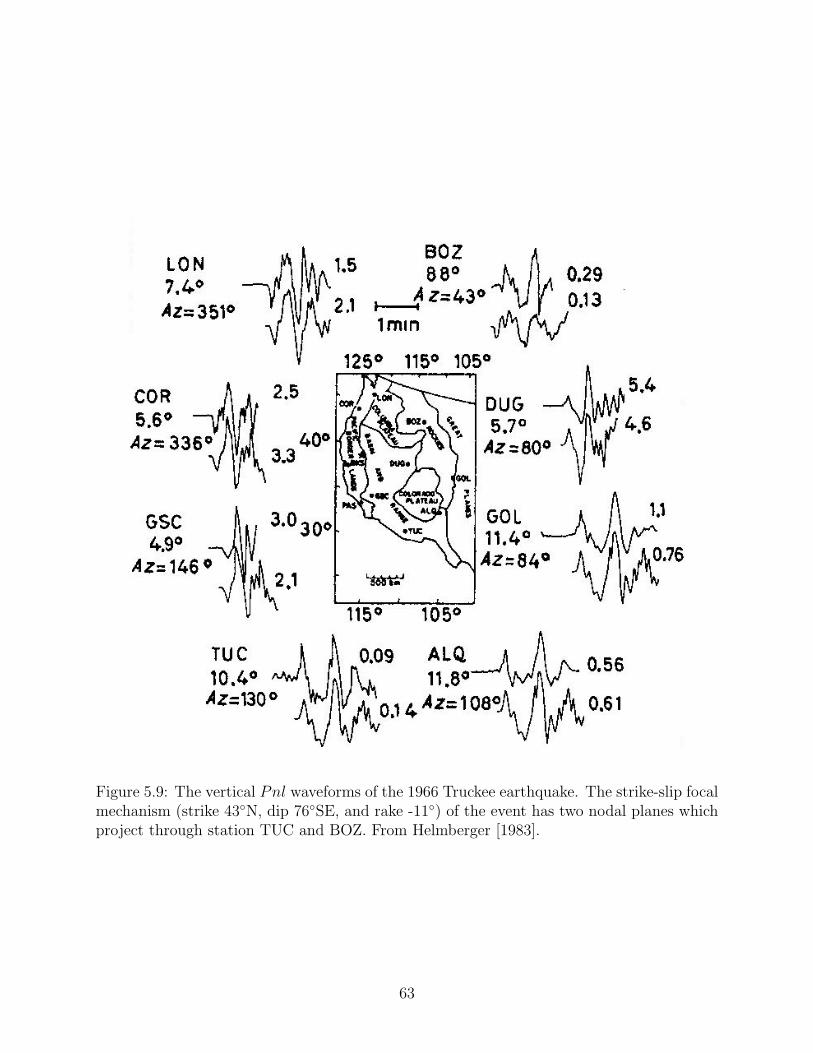
Figure 5.9: The vertical Pnl waveforms of the 1966 Truckee earthquake. The strike-slip focalmechanism (strike 43◦N, dip 76◦SE, and rake -11◦) of the event has two nodal planes whichproject through station TUC and BOZ. From Helmberger [1983].
63

Figure 5.10: Filtered data and synthetics from the Oroville earthquake. At all stations exceptGOL both the vertical (the first trace pair) and radial components are shown. The focalmechanism (strike 204◦, dip 66◦, rake 275◦) generates positive first-motions at all station inregional distances as opposed to those observed teleseismically. From Helmberger [1983].
64

Figure 5.11: Filtered data and synthetics for both the vertical and radial components froman earthquake in Turkey (strike 131◦, dip 68◦, rake 272◦). From Helmberger [1983].
65

Chapter 6
Upper-mantle Distance Waveforms
6.1 Earth flattening transformation
The Earth flattening transformation (EFT) transforms a sphere with constant velocity V0
to a half-space with variable velocity V (z) through
z = a lna
r, (6.1)
V (z) =a
rV0 = V0e
z/a. (6.2)
It can be shown that the above transformation gives the same travel-time at the sameepicentral distance for the half-space as for the sphere (kinematically equivalent).
It can be further shown that if we transform the density according
ρ(z) =(ra
)5
ρ0, (6.3)
the SH-waveform for the half-space is the same as for the sphere (dynamically equivalent)[Biswas and Knopoff, 1970]. For the P -SV system, there is no exact transformation [e.g.Chapman, 1973, Bhattacharya, 1996].
For a sphere with radially varying velocity and density, we can divide the sphere intomany thin shells and do EFT to each shell, using
dz =a
rdr. (6.4)
Fig. 6.1 shows IASPEI91 upper-mantle seismic velocity model before and after the Earthflattening transformation.
66

0
100
200
300
400
500
600
700
800
900
Z (
km)
3 4 5 6 7 8 9 10 11 12 13
V (km/s)
Figure 6.1: IASPEI91 upper-mantle seismic velocity model before the Earth flattening trans-formation (red lines) and after (black lines).
67

0
10
20
30
40
d (k
m)
0 1 2
t−d/6 (s)
Figure 6.2: Direct, reflected and head waves for a two liquid half-space model.
68

0
100
200
300
400
500
600
z (k
m)
0 500 1000 1500 2000x (km)
10
15
20
25
30
x (d
eg)
30 40 50 60
t-x/1060 70 80 90 100 110
t-x/5.5
Figure 6.3: P (left) and SH (right) triplicated waveforms due to the 410 discontinuity.
69

0100200300400500600700800
z (k
m)
0 500 1000 1500 2000 2500x (km)
10
15
20
25
30
x (d
eg)
30 40 50 60
t-x/1060 70 80 90 100 110
t-x/5.5
Figure 6.4: Triplicated P (left) and SH (right) waveforms for the IASPEI91 velocity model.
70

Figure 6.5: Vertical component seismograms going from Pnl domination at regional distancesto P and long-period at intermediate distances, a) strike-slip and b) dip-slip.
71

Figure 6.6: Comparison of synthetics with data of 9/12/1966 Truckee earthquake (strike 48◦,dip 80◦, and rake 0◦) at regional and upper-mantle distances. From Helmberger [1983].
72

6.2 Velocity discontinuity and triplication
6.3 Upper-mantle structure from modeling triplicated
waveforms
See Brudzinski and Chen [2003]
73

Chapter 7
Teleseismic Waveforms
7.1 Computing teleseismic synthetics
7.1.1 Full waveforms using normal-mode summation, DSM, andFK
7.1.2 Construction of teleseismic P -wave with GRT
uz =M0Rpz(p0)
4πρR
3∑j=1
Aj
[Cj(p0)δ(t) + Cj(p0)Rpp(p0)δ(t−∆t1) + SVj(p0)
ηα
ηβ
Rsp(p0)δ(t−∆t2)
].
(7.1)
7.2 Determining earthquake moment tensors and focal
depth
7.3 Determine upper mantle structure
See Tan and Helmberger [2006].
7.4 Teleseismic receiver functions
.
74

0
30
60
90
120
150
180
D (d
eg)
0 300 600 900 1200 1500 1800
t-D/18 (s)
P S
PcP ScS
PP SP SS
PKPdf SKSdf SKKSac
Figure 7.1: Vertical component record section of the 1994 Bolivia deep earthquake.
75

0
5000
10000
15000
Z (
km)
0 10 20 30 40 50 60 70 80 90 100 110 120
V (km/s)
Figure 7.2: IASPEI91 velocity model after EFT.
7.4.1 Computing receiver functions
The vertical and radial components of teleseismic P wave:
Z(t) = S(t)⊗ EZ(t), (7.2)
R(t) = S(t)⊗ ER(t), (7.3)
where S(t) is the time history of the incident P wave, which contains the earthquake sourcetime function and the propagation effect through the mantle. E(t)’s are the responses ofstructure beneath the seismic station. The above equations suggest that the local struc-ture responses can be isolated from three-component teleseismic recordings using spectrumdivision
R(ω)
Z(ω)=ER(ω)
EZ(ω). (7.4)
76
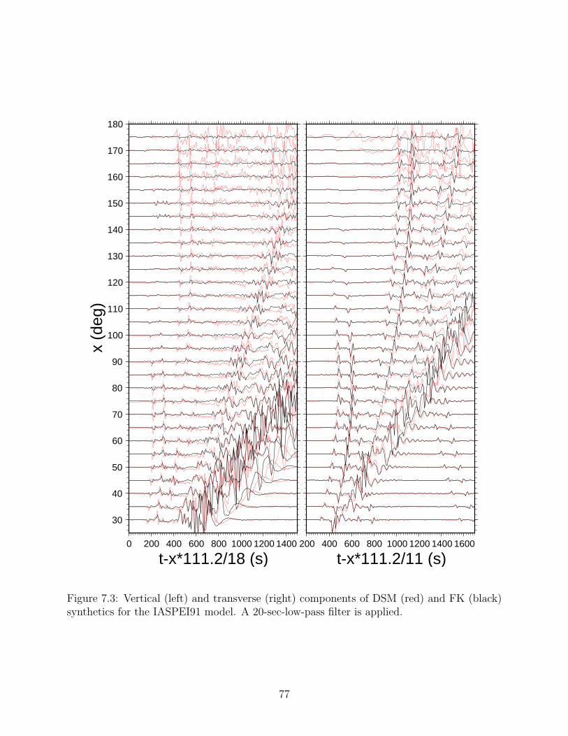
30
40
50
60
70
80
90
100
110
120
130
140
150
160
170
180
x (d
eg)
0 200 400 600 800 1000 1200 1400
t-x*111.2/18 (s)200 400 600 800 1000 1200 1400 1600
t-x*111.2/11 (s)
Figure 7.3: Vertical (left) and transverse (right) components of DSM (red) and FK (black)synthetics for the IASPEI91 model. A 20-sec-low-pass filter is applied.
77

30
40
50
60
70
80
90
100
110
120
130
140
150
160
170
180
x (d
eg)
0 200 400 600 800 1000 1200 1400
t-x*111.2/18 (s)200 400 600 800 1000 1200 1400 1600
t-x*111.2/11 (s)
Figure 7.4: Vertical (left) and transverse (right) components of normal-mode (red) and DSM(black) synthetics for the IASPEI91 model. A 20-sec-low-pass filter is applied.
78

The corresponding time sequence is called the receiver function [Langston, 1977].
r(t) =
∫R(ω)
Z(ω)ei ω tdω. (7.5)
Fig. 7.9 shows the vertical and radial responses of a simple crustal model and the correspond-ing receiver function for a incident teleseismic P wave with a ray parameter of 0.06 km/s.Receiver functions are dominated by P -to-S converted phases at various velocity interfaces(e.g. Moho) and their multiples.
Computing receiver functions can be done in the frequency domain (spectrum division)or time domain (Wiener filtering). Both methods pre-whiten the signal to suppress spectrum“holes” to make the computation stable, see the usage of program decon for details. Kikuchiand Kanamori [1982] introduced an iterative time-domain deconvolution method that workswell for noisy data. It has been implemented in program iter decn.
Some real examples of receiver functions at station PAS are shown in Fig. 7.10
7.4.2 Inversion for 1-D velocity structure
Receiver functions calculated from broadband seismic records contain many P -to-S con-verted phases produced by the crustal structure under the station. We can utilize a timedomain inversion technique [Owens et al., 1984, Ammon et al., 1990], which inverts thereceiver function for a one-dimensional velocity structure beneath the station. By using amatrix formalism for propagation of elastic waves in stratified medium, theoretical receiverfunctions and their partial differentials with respect to elastic parameters mi in each layercan be calculated [Kennett, 1983, Randall, 1989]. A set of linearized equations can then beconstructed from a Taylor expansion,
∂r(t)
∂mi
∆mi = robs(t)− rcal(t), (7.6)
which can be solved iteratively to get the one-dimensional velocity structure when the the-oretical receiver functions match the observations. Fig. 7.11 shows an example using atemporary station deployed on the Tibetan plateau [Zhu et al., 1993]. In general, such inver-sion results are very non-unique because receiver function waveforms are more sensitive tovelocity changes across discontinuities at different depths than to the velocities themselves.
7.4.3 Estimate crustal thickness and Vp/Vs ratio
Since Moho is usually the largest velocity discontinuity in the crust, the most prominentphase in the first 10 s of a radial receiver function is the Moho P -to-S conversion Ps. If wesimplify the crust as one layer with a P velocity of Vp and an S velocity of Vs, The time
79

separation between Ps and P can be used to estimate crustal thickness,
H =tPs√
1V 2
s− p2 −
√1
V 2p− p2
, (7.7)
where p is the ray parameter of the incident wave. An advantage of this method is thatbecause the P -to-S conversion point is close to the station (usually within 10 km laterally),the estimation is less affected by lateral velocity variations and thus provides a good pointmeasurement. One problem is the trade-off between the thickness and crustal velocities.However, since tPs represents the differential travel time of S with respect to P wave in thecrust, the dependence of H on Vp is not as strong as on Vs (or more precisely, on the Vp/Vs
ratio κ).
For example, using a Vp of 6.3 km/s and Vp/Vs ratio of 1.732 for a 30-km-thick crust, onegets
∆H =∂H
∂Vp
∆Vp = 4.3∆Vp (km),
which means that the uncertainty of H is less than 0.5 km for a 0.1 km/s uncertainty in Vp.However, the thickness is highly dependent on the Vp/Vs, as shown by
∆H =∂H
∂κ∆κ = −40.2∆κ (km),
i.e., a 0.1 change in κ can lead to about 4 km change in the crustal thickness. This ambiguitycan be reduced by using the later phases which provide additional constraints
H =tPpPs√
1V 2
s− p2 +
√1
V 2p− p2
, (7.8)
H =tPpSs+PsPs
2√
1V 2
s− p2
, (7.9)
so that both κ and H can be estimated [Zhu, 1993, Zandt et al., 1995, Zandt and Ammon,1995].
In real situations, identifying the Moho Ps and the multiples and measuring their ar-rival times on a single receiver function trace can be very difficult due to background noise,scatterings from crustal heterogeneities, and P -to-S conversions from other velocity discon-tinuities. To increase the signal/noise ratio (SNR), one can use multiple events to stacktheir receiver functions. Such stacking is usually done in the time domain for a cluster ofevents [e.g., Owens et al., 1984]. Zhu and Kanamori [2000] proposed a straightforward H-κdomain stacking defined as
s(H, κ) = w1r(t1) + w2r(t2)− w3r(t3), (7.10)
where r(t) is the radial receiver function, t1, t2 and t3 are the predicted Ps, PpPs, andPpSs+PsPs arrival times corresponding to crustal thickness H and Vp/Vs ratio κ, as given
80
in (7.7)–(7.9). The wi are weighting factors, and∑wi = 1. The s(H, κ) reaches a maxi-
mum when all three phases are stacked coherently with the correct H and κ (Figure 7.12).Advantages of this algorithm are that (1) large amounts of teleseismic waveforms can beconveniently processed; (2) there is no need to pick arrival times of different conversionphases; (3) by stacking receiver functions from different distances and directions, effects oflateral structure variation are suppressed and an average crustal model is obtained; and (4)uncertainties can be estimated from the flatness of s(H, κ) at the maximum.
7.4.4 CCP stacking and imaging
Zhu [2000] developed a stacking and imaging technique called Common Conversion Point(CCP) stacking technique to image crustal structure when multiple stations are deployedclose to each other so that the teleseismic rays to them crisscross in the crust. First theray-path of the receiver function is calculated using a background velocity model. Thenthe amplitude at each point on the receiver function, after corrected for the incidence angleeffect, is assigned to the corresponding location on the ray-path where the P -to-S conversionoccurred, using its time delay with respect to the direct P . This amplitude represents thevelocity change, or more precisely the impedance change, of the medium at the conversionpoint. The crustal volume is divided into certain size bins and all amplitudes in each bin aresummed to obtain the average amplitude and variance. Fig. 7.13 shows a CCP image alonga 140-km-long profile across the San Andreas Fault in southern California from stacking 941short-period receiver functions.
7.5 Core phases
81
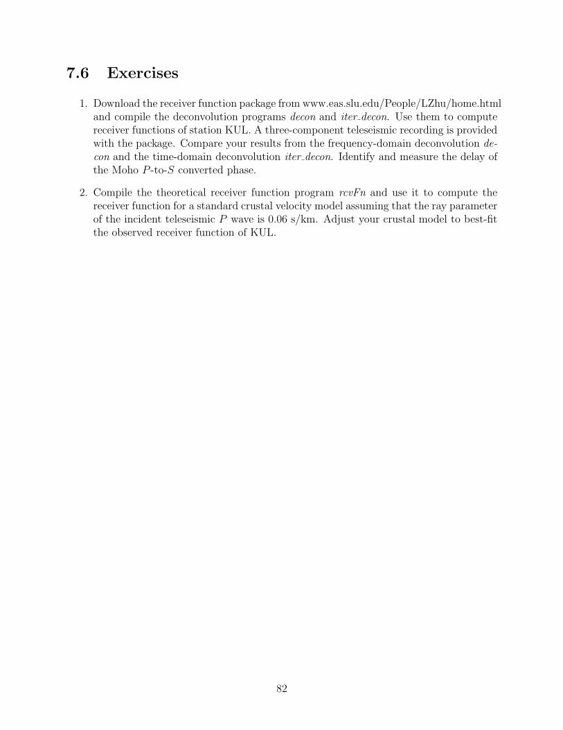
7.6 Exercises
1. Download the receiver function package from www.eas.slu.edu/People/LZhu/home.htmland compile the deconvolution programs decon and iter decon. Use them to computereceiver functions of station KUL. A three-component teleseismic recording is providedwith the package. Compare your results from the frequency-domain deconvolution de-con and the time-domain deconvolution iter decon. Identify and measure the delay ofthe Moho P -to-S converted phase.
2. Compile the theoretical receiver function program rcvFn and use it to compute thereceiver function for a standard crustal velocity model assuming that the ray parameterof the incident teleseismic P wave is 0.06 s/km. Adjust your crustal model to best-fitthe observed receiver function of KUL.
82

Figure 7.5: Teleseismic P -wave synthetics. The source time functions are (0.5, 1.0, 0.5) secsfor high stress-drop, (1.0, 3.0, 1.0) secs for medium stress-drop, and (2.0, 6.0, 2.0) for lowstress-drop. From Helmberger [1983].
83

Figure 7.6: Observed (top) and synthetic (bottom) long-period P waveforms at 14 WWSSNstations from the Borrego Mtn. earthquake. From Helmberger [1983].
84

Figure 7.7: Observed (top) and synthetic (bottom) long-period P waveforms from theOroville earthquake on Aug. 1, 1975 (strike 180◦, dip 65◦, rake -70◦). From Helmberger[1983].
85

Figure 7.8: Observed (top) and synthetic (bottom) vertical long-period WWSSN P wave-forms from the Bermuda earthquake on March 24, 1978. From Helmberger [1983].
86

0 10 20 30
t (s)
Vertical
Radial
r(t)
Ps PpPms
PpSms+PsPms
Moho
PsPpPm
s
Figure 7.9: Receiver functions of a one-layer crustal model. The ray parameter of the incidentP wave is 0.06 km/s.
87
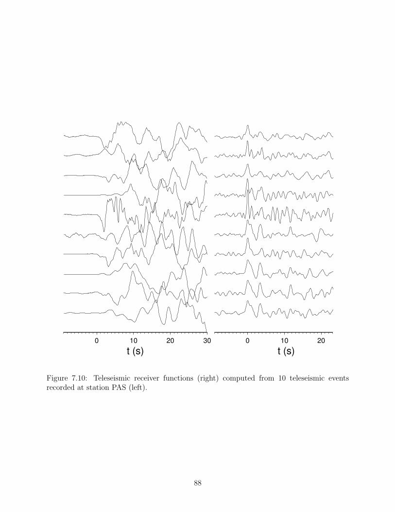
0 10 20 30
t (s)0 10 20 30
t (s)
Figure 7.10: Teleseismic receiver functions (right) computed from 10 teleseismic eventsrecorded at station PAS (left).
88

Figure 7.11: Inversion results using receiver functions of WNDO from SE. (a) Initial (dashedline) and final (solid line) shear velocity models. (b) the fit of final synthetic receiver function(dashed line) to both the mean receiver function (solid line) and the bounds (c).
89

0.04
0.05
0.06
0.07
0.08
p (s
/km
)
0 5 10 15 20
t (s)
Ps PpPs
PpSs+PsPs
1.60
1.65
1.70
1.75
1.80
1.85
1.90
κ
0.00
0.05
0.10
0.15
0.20(a)
1.60
1.65
1.70
1.75
1.80
1.85
1.90
κ
15 20 25 30 35 40
H (km)
Ps PpPs
PpSs+PsPs
(b)
Figure 7.12: The left panel shows radial receiver function as a function of ray parameter pfor the Standard Southern California Velocity Model. Right: (a) The s(H, κ) from stackingthe receiver functions using (7.10). It reaches the maximum (solid area) when the correctcrustal thickness and Vp/Vs ratio are used in the stacking. (b) H-κ relations, as given in(7.7)–(7.9), for different Moho converted phases. Each curve represents the contributionfrom this converted phase to the stacking.
90

-50
-40
-30
-20
-10
0D
epth
(km
)
-40 -30 -20 -10 0 10 20 30 40 50 60 70 80 90 100
0.1
0.1
0.10.1
0.1
0.2
0.2
0.2
0.2
SA
F
ECSZMojave Desert
ALAB
-0.15 -0.10 -0.05 0.00 0.05 0.10 0.15
Amplitude
-50
-40
-30
-20
-10
0
Dep
th (
km)
-40 -30 -20 -10 0 10 20 30 40 50 60 70 80 90 100
SA
F
SM
F
ECSZ
VC
T
Upper Crust
Lower Crust
Upper Mantle
Moho
Mojave Desert
B
LAB
-120
-100
-80
-60
∆g (
mga
l)
Figure 7.13: (A) The amplitude and variance (given by the contours) of CCP stacking. Novertical exaggeration except that the surface topography is amplified by a factor of 2. SAF:San Andreas Fault; LAB: Los Angeles Basin. (B) Crustal structure along the profile basedon A. The thickened black lines are Moho and other possible velocity discontinuities. SMF:Sierra Madre Fault; VCT: Vicent Thrust Fault. Red crosses are earthquakes within the pro-file between 1981 and 1998. Green lines are the crustal reflectors imaged by LARSE [Rybergand Fuis, 1998]; Hatched area in the upper mantle represents the Transverse Range highvelocity anomaly from seismic tomography [Humphreys and Clayton, 1990]. Plotted on thetop are the observed Bouguer gravity anomaly and the predicted Bouguer anomalies usingthe determined Moho topography (dashed line) and the Airy isostasy model (dotted line).91

0
5000
10000
15000
z (k
m)
0 5000 10000 15000x (km)
ab
bc&cd
df
120
125
130
135
140
145
150
155
160
165
170
x (d
eg)
860 870 880 890 900 910 920 930 940
t-x*111.2/60 (s)
a
b
c
d
f
Figure 7.14: Vertical component of GRT synthetic seismograms for the IASPE91 model.
92

155
160
165
170
x (d
eg)
0 10 20 30 40 50 60 70
t (s)
Figure 7.15: Comparison between observed (red) and synthetic vertical component of velocityrecords from the 6/29/2001 Mw 6.1 earthquake.
93

Bibliography
D. V. Helmberger. Theory and application of synthetic seismograms. In Earthquakes: Ob-servation, Theory and Interpretation, pages 174–222. Soc. Italiana di Fisica, Bolgna, Italy,1983.
K. Aki and P. G. Richards. Quantitative Seismology, Theory and Methods. Freeman andCompany, San Francisco, 1980.
L. Zhu. Recovering permanent displacements from seismic records of the June 9, 1994 Boliviadeep earthquake. Geophys. Res. Lett., 30(14):1740, doi:10.1029/2003GL017302, 2003.
J. E. Vidale, S. Goes, and P. G. Richards. Near-field deformation seen on distant broadbandseismograms. Geophys. Res. Lett., 22:1–4, 1995.
T. Ryberg and G.S. Fuis. The San Gabriel Mountains bright reflective zone: possible evidenceof young mid-crustal thrust faulting in southern California. Tectonophys., 286(1-4):31–46,1998.
E.D. Humphreys and R.W. Clayton. Tomographic image of the southern California mantle.J. Geophys. Res., 95(B12):19725–19746, 1990.
L. Knopoff and M. J. Randall. The compensated linear-vector dipole: a possible mechanismfor deep earthquake. J. Geophys. Res., 75:4957–4963, 1970.
M. L. Jost and R. B. Herrmann. A student’s guide to and review of moment tensors. Seismol.Res. Lett., 60:37–57, 1989.
J. A. Hudson, R. G. Pearce, and R. M. Rogers. Source type plot for inversion of the momenttensor. J. Geophys. Res., 94:765, 1989. doi: 10.1029/JB094iB01p00765.
C. H. Chapman and W. S. Leaney. A new moment-tensor decomposition for seismicevents in anisotopic media. Geophys. J. Int., 188:343–370, 2011. doi: 10.1111/j.1365-246X.2011.05265.x.
T. W. Spencer. The method of generalized reflection and transmission coefficients. Geo-physics, 25:625–641, 1960.
D. V. Helmberger. The crust-mantle transition in the Bering Sea. Bull. Seismol. Soc. Am.,58:179–214, 1968.
94

H. Takeuchi and M. Saito. Seismic surface waves. In B. A. Bolt, editor, Methods in Compu-tational Physics, volume 11, pages 217–295. Academic Press, New York, 1972.
H. W. Turnbull and A. C. Aitken. An introduction to the theory of canonical matrices.Blackie and Son, Ltd., London and Glasgow, 1952.
F. R. Gantmatcher. Matrix Theory. Chelsea Publishing Company, New York, N. Y., 1960.
N. A. Haskell. Radiation pattern of surface waves from point sources in a multi-layeredmedium. Bull. Seismol. Soc. Am., 54:377–393, 1964.
C. Y. Wang and R. B. Herrmann. A numerical study of P, SV, and SH-wave generation ina plane layered medium. Bull. Seismol. Soc. Am., 70:1015–1036, 1980.
N. A. Haskell. The dispersion of surface waves on multilayered media. Bull. Seismol. Soc.Am., 43:17–34, 1953.
M. Bouchon. A simple method to calculate green’s function for elastic layered media. Bull.Seismol. Soc. Am., 71:959–971, 1981.
C. K. Saikia. Modified frequency-wavenumber algorithm for regional seismograms usingfilon-quadrature method – modeling of Lg waves in eastern North-America. Geophys. J.Int., 118:142–158, 1994.
R. B. Herrmann. Seismic Wave in Layered Media.http://http://www.eas.slu.edu/People/RBHerrmann/CPS330.html, 2007.
L. Zhu and L. A. Rivera. A note on the dynamic and static displacements from a pointsource in multi-layered media. Geophys. J. Int., 148:619–627, 2002.
P. Molnar and W. P. Chen. Focal depths and fault plane solutions of earthquakes under theTibetan plateau. J. Geophys. Res., 88:1180–1196, 1983.
N. N. Biswas and L. Knopoff. Exact earth-flattening calculation for Love waves. Bull.Seismol. Soc. Am., 60:1123–1137, 1970.
C. H. Chapman. The earth flattening transformation in body wave theory. Geophys. J. R.astr. Soc., 35:55–70, 1973.
S. N. Bhattacharya. Earth-flattening transformation for P-SV waves. Bull. Seismol. Soc.Am., 86:1979–1982, 1996.
M. R. Brudzinski and Wang-Ping Chen. A petrologic anomaly accompanying outboard earth-quakes beneath Fiji-Tonga: Corresponding evidence from broadband P and S waveforms.J. Geophys. Res., 108:2299,doi:10.1029/2002JB002012, 2003.
Y. Tan and D. V. Helmberger. Trans-pacific upper mantle shear velocity structure. J.Geophys. Res., submitted, 2006.
95

C. A. Langston. The effect of planar dipping structure on source and receiver responses forconstant ray parameter. Bull. Seismol. Soc. Am., 67:1029–1050, 1977.
M. Kikuchi and H. Kanamori. Inversion of complex body waves. Bull. Seismol. Soc. Am.,72:491, 1982.
T. J. Owens, G. Zandt, and S. R. Taylor. Seismic evidence for ancient rift beneath the Cum-berland plateau, Tennessee: A detailed analysis of broadband teleseismic P waveforms. J.Geophys. Res., 89:7783–7795, 1984.
C. J. Ammon, G. E. Randall, and G. Zandt. On the nonuniqueness of receiver functioninversions. J. Geophys. Res., 95:15,303–15,318, 1990.
B. Kennett. Seismic wave propagation in stratified media. Cambridge University Press, 1983.
G. E. Randall. Efficient calculation of differential seismograms for lithosphere receiver func-tions. Geophys. J. Int., 99:469–481, 1989.
L. Zhu, R. S. Zeng, F. T. Wu, T. J. Owens, and G. E. Randall. Preliminary study ofcrust-upper mantle structure of the Tibetan plateau by using broadband teleseismic bodywaveforms. Acta Seismol. Sinica, 6:305–315, 1993.
L. Zhu. Estimation of crustal thickness and Vp/Vs ratio beneath the Tibetan Plateau fromteleseismic converted waves. Eos Trans. AGU, 74(16):Spring Meeting Suppl., 202, 1993.
G. Zandt, S. C. Myers, and T. C. Wallace. Crust and mantle structure across the Basinand Range-Colorado Plateau boundary at 37N latitude and implications for Cenozoicextensional mechanism. J. Geophys. Res., 100:10529–10548, 1995.
G. Zandt and C. J. Ammon. Continental-crust composition constrained by measurementsof crustal Poissons ratio. Nature, 374:152–154, 1995.
L. Zhu and H. Kanamori. Moho depth variation in southern California from teleseismicreceiver functions. J. Geophys. Res., 105:2969–2980, 2000.
L. Zhu. Crustal structure across the San Andreas Fault, southern California from teleseismicconverted waves. Earth Planet. Sci. Lett., 179:183–190, 2000.
96