synthetic seismograms using a hybrid broadband … seismograms using a hybrid broadband...

Synthetic Seismograms Using a Hybrid Broadband Ground-Motion

Simulation Approach: Application to Central

and Eastern United States

by Alireza Shahjouei and Shahram Pezeshk

Abstract Broadband synthetic time histories for central and eastern United Statesare generated using a proposed hybrid broadband simulation technique. The low-frequency (LF) portion of synthetics is calculated using kinematic source modelingand deterministic wave propagation. Using the COMPSYN software package (Spu-dich and Xu, 2003), a discrete wavenumber/finite-element method is implemented forthe LF Green’s functions generation. The procedure makes use of the reciprocity theo-rem and numerical techniques to assess the representation theorem integrals on a faultsurface. Spatial random field models are employed to characterize the complexity ofthe slip distribution on the heterogeneous fault. In this study, the variability of some ofthe kinematic source modeling’s parameters (e.g., hypocenter locations, slip distribu-tion, source time function, and rupture propagation) is taken into account to producemultiple seismograms that contain a broader range of intensity measures such as peakground motions and spectral accelerations. A stochastic finite-fault simulation modelis employed to attain the high-frequency (HF) portion of synthetics. Combining HFand LF synthetics in a magnitude-dependent transition frequency, the broadband seis-mograms are constructed forM 5.5,M 6.5, andM 7.5 earthquakes in a distance rangeof 2–200 km.

Broadband synthetics will be compared with some of the existing ground-motionprediction equations for spectral accelerations at 0.2, 1.0, and 3.0 s, and the results willbe discussed. A compatibility assessment of the stochastic point source and the finitesource is performed. The generated seismograms could be implemented in engineer-ing seismology applications such as structural seismic analysis/design and seismic-hazard analysis.

Introduction

Generation of accurate synthetic seismograms in the ab-sence of the appropriate recorded strong ground motions hasbeen a challenging issue in the fields of earthquake engineer-ing and engineering seismology. According to the buildingcodes, a number of either recorded and/or synthetic seismo-grams is needed for the seismic time history analysis ofunique and irregular structures (Baker, 2011; Ghodrati et al.,2011). In addition, synthetic seismograms may be consideredas a complement to the available earthquake catalog and canbe used to develop ground-motion prediction equations(GMPEs), particularly in the regions with historical seismic-ity but insufficient recorded strong ground motions (Pezeshket al., 2011). In general, these ground-motion models inwell-recorded regions are empirically developed from therecorded earthquakes. Examples of such empirical GMPEsare ground-motion models for western North America devel-oped by Graizer and Kalkan (2007) and Boore et al. (2014).

The synthetic seismograms should include the specificunderlying seismological features of a region and have char-acteristics of the frequency content, shaking duration, pulse-like character, and peak ground motions compatible with therecorded data at a site (Frankel, 2009).

In general, all main characteristics of an earthquake timehistory (amplitude, frequency content, and duration) signifi-cantly contribute to and have influence on the structuralresponse values, the seismic risk analysis, and the seismicdamage assessment (Hartzell et al., 1999). Although a pre-cise prediction of future large earthquakes in time, location,and the time history—wiggle for wiggle—is not possiblenowadays, some of the seismological and geological infor-mation could be implemented to characterize the earthquakesource, the path effect, and the site characteristic and todetermine the potential of future damaging earthquakes(Liu et al., 2006). All this information is the basis for the

686

Bulletin of the Seismological Society of America, Vol. 105, No. 2A, pp. 686–705, April 2015, doi: 10.1785/0120140219

development of empirical equations and is used in earth-quake simulation techniques.

In the literature, a number of engineering-based, as wellas seismological-based approaches have been proposed re-lated to ground-motion simulation. Most engineering-basedtechniques have been focused on the ground-motion spectrummatching with a desired (design or target) spectrum (Suarezand Montejo, 2007; Ghodrati et al., 2011; Malekmohammadi,2013). The target spectrum may be derived from a probabilisticseismic-hazard analysis (Baker, 2011; Malekmohammadi,2013). Seismological-based techniques, instead, construct thesynthetics by either dynamic, kinematic, or stochastic model-ing of the earthquake source.

The stochastic point-source simulation is a popularmethod for generating high-frequency (HF) ground motions(Boore, 1983). The stochastic approaches (either pointsource or finite source) generate seismograms by consideringa random process for ground motions over almost allfrequencies (Boore, 2003). The stochastic point-source tech-niques (such as the SMSIM software by Boore, 2005, 2012)and the stochastic finite-fault methods (such as the EXSIMsoftware by Motazedian and Atkinson, 2005) are widelyused to generate synthetic seismograms in both engineeringand seismological applications. Atkinson et al. (2009) andBoore (2009) provided informative and detailed discussionson the comparison of the stochastic finite-source and the sto-chastic point-source models.

Dynamic models and kinematic models are two ap-proaches for modeling of an earthquake source to predictmore precise ground motions having the underlying physicalmechanism. The kinematic source model assumes a specificslip distribution as well as a source time function (STF),whereas in the dynamic model an explicit frictional failurelaw (e.g., slip-weakening model) is specified (Trugmanand Dunham, 2014). As the computational problem of therupture process in dynamic models is nonlinear, such modelsare computationally more intensive than kinematic models.The pseudodynamic (PD) model is an alternative to the dy-namic model in which the main physical characteristics ofthe rupture simulation are related to the kinematic modelto develop dynamically consistent kinematic source modelsthat are computationally more efficient. Examples of incorpo-rating PD source models in ground-motion simulations may befound in studies by Guatteri et al. (2004), Song and Somer-ville (2010), Mena et al. (2012), Schmedes et al. (2013), Songet al. (2014), and Trugman and Dunham (2014).

The deterministic simulation of the ground motion usingdynamic, pseudodynamic, and kinematic approaches in abroad frequency range of engineering interest (0–10 Hz) isstill computationally expensive (Schmedes et al., 2013).Hybrid broadband (HBB) simulation techniques have beendeveloped in which the deterministically generated long-period synthetics are combined with HF motions to producebroadband synthetics for the entire frequency band ofinterest. Some of the broadband methods (e.g., Zeng et al.,1994; Hartzell et al., 2005; Mai et al., 2010) use the physics

of wave scattering to simulate the HF ground motion(frequency > 1:0 Hz), whereas some other methods incor-porate stochastic approaches to generate the HF portion ofseismograms (e.g., Graves and Pitarka, 2004, 2010; Liu et al.,2006; Frankel, 2009). In the first group, Zeng et al. (1994)proposed a HBB composite source model, which uses scatter-ing functions for HF coda waves. Hartzell et al. (2005) calcu-lated broadband time histories using kinematic and dynamicmodels and compared the results with the 1994 Northridgeearthquake. Mai et al. (2010) combined the low-frequency(LF) deterministic seismograms (frequency < 1:0 Hz) withthe HF S-to-S backscattering seismograms. Mena et al. (2010)updated Mai et al. (2010) by accounting for finite-fault effectsin HF wave computation, as well as applying dynamicallyconsistent STFs in the simulation. In the latter methods,Liu et al. (2006) generated the broadband ground-motionsynthetics using a frequency method with correlation randomsource parameters. Frankel (2009) proposed a constantstress-drop model to generate HBB synthetic seismograms.He also used a static stress drop for HF synthetics and dy-namic stress drop for LF synthetics in his simulations. Gravesand Pitarka (2010) updated the hybrid simulation approachof Graves and Pitarka (2004) by incorporating spatial hetero-geneity in slip, rupture speed, and rise time in the kinematicrupture fault modeling.

The central and eastern United States (CEUS) is consid-ered a high seismic area where recorded strong ground mo-tions are scarce. Hwang et al. (2001) generated syntheticseismograms from the large New Madrid earthquake using astochastic method. Somerville et al. (2001) generated broad-band synthetics to develop GMPEs for CEUS. Olsen (2012)implemented 3D broadband simulations to predict groundmotions in the New Madrid Seismic Zone (NMSZ) for1811–1812 events with the moment magnitudes M 7.4–7.7earthquakes. Synthetic simulations are also performed inthe studies of Frankel et al. (1996), Toro (2002), Campbell(2003), Tavakoli and Pezeshk (2005), Atkinson and Boore(2006), and Pezeshk et al. (2011) to develop ground-motionmodels in central and eastern North America.

The objective of this study is to generate synthetic seis-mograms the characteristics of which are consistent with theoverall characteristic of ground motions expected to observein CEUS. Applying the proposed broadband approach, seis-mograms are produced from different shaking scenarios forthis region. The key feature of this study is implementing thediscrete wavenumber/finite-element (DWFE) technique of theCOMPSYN package (Spudich and Xu, 2003) to compute LFsynthetics in the proposed broadband simulation approachfor CEUS. In addition, the most recently updated geologicaland seismological parameters (of both kinematic and sto-chastic source modeling) and techniques that are proposedin the literature and are compatible with CEUS are incorpo-rated in earthquake simulations. The HF synthetics are com-puted through the stochastic finite-fault method applyingidentical fault planes defined and implemented in LF simu-lations. We used the updated seismological parameters in

Synthetic Seismograms Using a Hybrid Broadband Ground-Motion Simulation Approach: Application to CEUS 687

CEUS in HF synthetic simulations. The LF and HF syntheticsare combined in a magnitude-dependent transition frequencyto construct the broadband synthetics. The simulationapproach is implemented to generate synthetics for three mo-ment magnitudes of M 5.5, M 6.5, and M 7.5 at the source–station distance range of 2–200 km for hard-rock conditionsin CEUS. Spectrum compatibility of the synthetics is pre-sented to validate the method. The response spectral ampli-tudes from the synthetics are compared with those obtainedfrom some of the recent GMPEs for CEUS.

Hybrid Broadband Simulation Method

In the proposed hybrid simulation technique, HF and LFground-motion synthetics are separately calculated and thencombined to produce broadband time histories. A transitionfrequency between HF and LF portions in many studies ispresumed to be around 1.0 Hz. Frankel (2009) proposed amagnitude-dependent transition frequency based on his ob-servation of the magnitude dependency of the transition offrequency between coherent and incoherent summation inrecorded earthquakes. Following Frankel (2009), we imple-mented transition (crossover) frequencies of 0.8, 2.4, and3.0 Hz in our simulations for moment magnitudes (M) of7.5, 6.5, and 5.5, respectively.

The LF and HF synthetics are combined after passingmatched filters. To combine two portions of synthetics ateach station, HF synthetic (generated in frequencies greaterthan transition frequency) is synchronized with LF synthetics(generated in frequencies lower than transition frequency)applying the real arrival time computed in LF simulations.Second-order low-pass and high-pass Butterworth filters areimplemented to the deterministic LF and stochastic HFsynthetics, respectively. These phaseless filters have similarfall-offs and corner frequencies and do not vary the phase ofthe synthetics (Hartzell et al., 1999). Figure 1 illustrates theflowchart of the simulation approach. Detailed discussionsare provided in the next few sections.

Low-Frequency Simulation

Low-frequency synthetics are constructed using thekinematic source modeling of the earthquake fault and thedeterministic wave propagation approach. The detailedsource characterizations and the wave propagation are de-scribed next.

Kinematic Source Characteristics. A kinematic earthquakesource model is implemented to generate LF synthetics. Themain input parameters are the fault geometry (length, width,dip, and strike) and the location, a desired magnitude (mo-ment magnitude or seismic moment), a hypothetical ruptureinitiation point on the fault surface (the hypothetical hypo-center), the slip direction (rake), and the crustal model of theearth at the vicinity of the fault. The average of slip on thefault, D, is estimated by

D � M0

μA; �1�

in whichM0 is the seismic moment, μ is the rigidity, and A isthe rupturing area. The shear modulus μ � 3:3 × 1010 N=m2

is used in this study. A random slip distribution on the faultwith a wavenumber-squared spectral decay (k2) is assumed(Somerville et al., 1999; Graves and Pitarka, 2010). Theheterogeneity of the slip distribution on the fault is modeledusing different spatial random fields proposed by Mai andBeroza (2002) and Frankel (2009). We used the von Karmanautocorrelation function (ACF) of Mai and Beroza (2002).The detailed description of this function is also briefly de-scribed in the Appendix. The slip distribution is scaled tomatch the desired moment for the entire faulting rupture,which is calculated using equation (1).

Assuming a hypothetical hypocenter on a fault, the rup-ture arrival time on each point of the fault is determinedfollowing modifications of Graves and Pitarka (2010). Theprocedure includes calculation of a background rupturespeed distribution and local slip-dependent scaling steps. Inthe first step, a general ratio of the rupture velocity (VR) tothe local shear velocity (VS), (i.e.,VR=VS) is assumed to be

Crustal modelFaulting Mech.

Desired MFaulting AreaStation map

LF Green’s functions(DWFE method ~ COMPSYN)

Slip distribution

Kinematic fault modeling

Stress distribution

HF Green’s functions(Stochastic method ~ SMSIM)

Low -freq. synth.(Sum over fault plane)

High f- req. synth.(Sum over fault plane, andscaling with magnitude)

Hybrid broadband synthetic Synchronize

CombineMatched filter

Max directional response(GMROT)

Figure 1. Flowchart of the method used to compute hybrid broadband (HBB) synthetics. The color version of this figure is available onlyin the electronic edition.

688 A. Shahjouei and S. Pezeshk

0.8 on the deeper part of the fault (Somerville et al.,1999), and a 70% reduction on the shallower part (i.e.,VR � 0:56VS) is applied to represent the shallow weak zonein the surface-rupture events (Pitarka et al., 2009). The back-ground rupture velocity distribution is given by equation (2).The linear interpolation is used between the depth (z) of 5and 8 km. Equation (2) is used to calculate the initial rupturefront arrival time, TR0−i at any individual subfault, i (Gravesand Pitarka, 2004, 2010):

VR ��0:8 × VS z > 8 km0:56 × VS z < 5 km

: �2�

The final rupture arrival time TRF−i at each subfault, i, afterscaling is determined as

TRF−i � TR0−i − Δt�log�si� − log�sA�log�sM� − log�sA�

�; �3�

in which SA and SM are the average and the maximum slip onthe fault, respectively. Si is the local slip at subfault, i. Thescaling factor Δt � 1:8 × 10−9 ×M1=3

0 is applied followingGraves and Pitarka (2010). We added a small random compo-nent (no more than 5%) to the final rupture front values TRF−i.

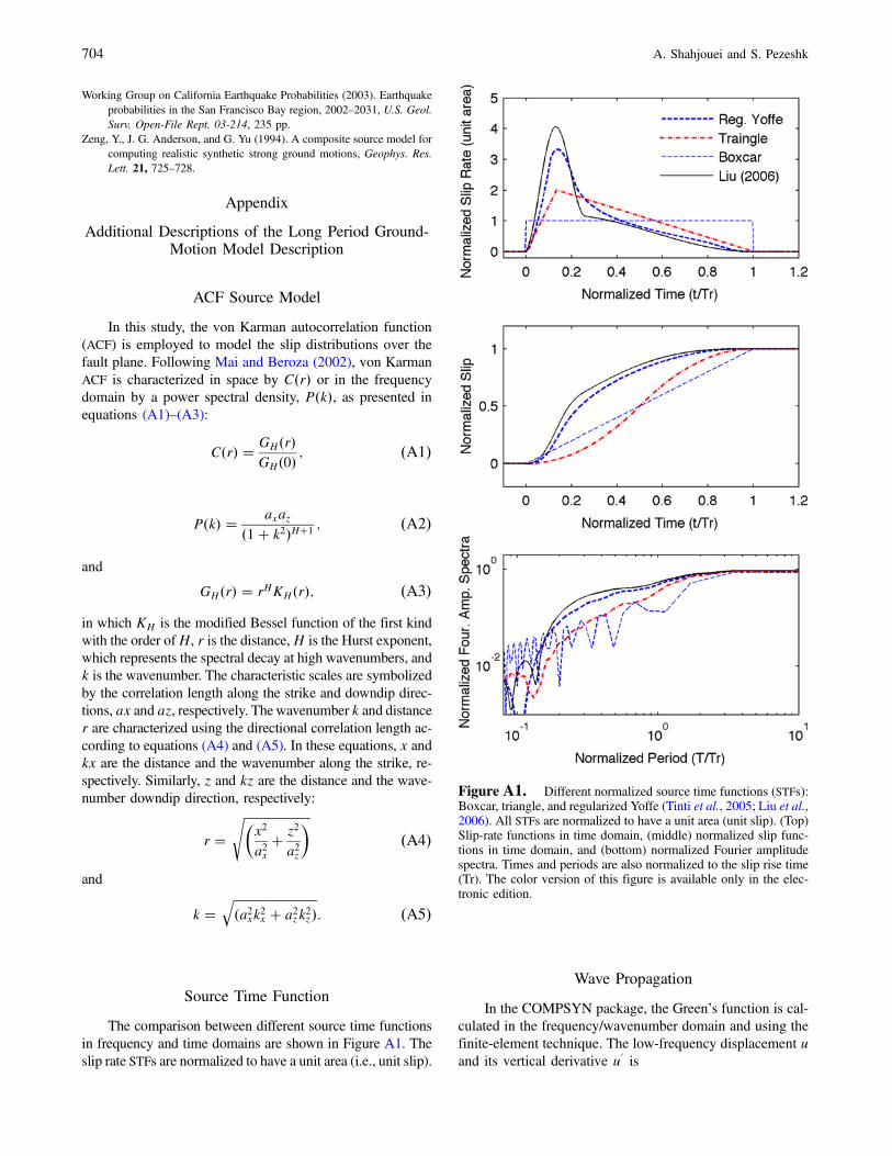
One of the assumption requirements in the kinematicearthquake source model is defining the time history of thefinite slip duration during the rupture propagation. Tinti et al.(2005) performed a broad study on the STFs, and they pro-posed a kinematic regularized Yoffe slip rate function com-patible with earthquake dynamics. Liu et al. (2006) proposeda trigonometric slip velocity function. Figure A1 shows thecomparison of a number of kinematic slip rate functions inboth time and frequency domains. In this study, we em-ployed boxcar, triangle, and the Liu et al. (2006) STFs indifferent simulations. Graves and Pitarka (2010) proposeda function to heterogeneously distribute the rise time (dura-tion of slip rate function) over the fault. The function is givenin equation (4) with a linear transition between depths of 5and 8 km. It incorporates the effect of reductions in peak sliprates in the shallower depth of surface-rupturing events (byapplying factor 2 in z < 5 km) and represents the trade-offbetween using constant rise time and constant slip velocity—by applying S0:5:

TR−i ��k × S0:5i z > 8 km2 × k × S0:5i z < 5 km

�4�

(Aagaard et al., 2008), in which TR−i and Si are the local risetime and the local slip at subfault i. We calculated the con-stant k such that the average rise time in the asperity regionsover the fault is equal to the suggested value for the region.Somerville et al. (1999, 2009) proposed an average rise timefor CEUS. A dip-dependent modification factor on the aver-age rise time was proposed by Graves and Pitarka (2010).This modification reduces the rise time by decreasing thefault dip. The resultant relation for the CEUS region is givenin equations (5) and (6):

τ � ατ × 3 × 10−9 ×M1=30 ; �5�

in which τ is the average rise time, ατ is the scale that is afunction of fault dip, δ, and the seismic moment, M0, hasdyn·cm unit. A linear transition is applied between dips45° and 60°. The ατ modification is consistent with observa-tions for thrust- and reverse-faulting events (Hartzell et al.,2005) and should not be used on the normal-faulting scenar-ios (Graves and Pitarka, 2010):

ατ ��1:0 δ > 60°0:82 δ < 45°

: �6�

We added a random component to equation (5) and con-strained the average rise time not to vary more than 5%of the average value.

Deterministic Wave Propagations. The complete long-period Green’s functions for the wave propagation througha layered crustal velocity model are calculated using theDWFE method of Olson et al. (1984), applying the COMP-SYN codes by Spudich and Xu (2003). The COMPSYNpackage has been widely used in the literature for earthquakesimulation applications (e.g., Ameri et al., 2008; Rippergeret al., 2008; Wang et al., 2009; Mena et al., 2012). To evalu-ate the representation theorem integrals on the fault surface, thepackage uses the numerical techniques of Spudich and Arch-uleta (1987). In this package, the earth is assumed in a 3DCartesian space with a free surface at z � 0. The applicationadopts the crustal structure as a 1D layered elastic medium;therefore, anelastic attenuation and 3D basin effects is not con-sidered in the computation. Because the anelastic attenuationeffect at near distances is not significant, this approximationdoes not notably affect the results (Ameri et al., 2008).

A midcontinent crustal model suggested for CEUS byMooney et al. (2012) and W. Mooney (personal comm.,2013) was used in the study. We incorporated the crustalvelocity model at shallow depths (to a depth of 1 km) follow-ing Somerville et al. (2001). Table 1 summarizes the crustalstructure model used in this study.

Long-period synthetic seismograms are generated com-putationally fairly quickly compared with the 3D codes andinclude the complete response of the earth structure (i.e.,P and S waves, surface waves, leaky modes, and near-field

Table 1The Midcontinent Crustal Structure Model, Which isUsed in Simulations for central and eastern United

States (CEUS)

Z (km) VP (km=s) VS (km=s) ρ (g=cm3)

0.0 4.9 2.83 2.521.0 6.1 3.52 2.7410.0 6.5 3.75 2.8320.0 6.7 3.87 2.8840.0 8.1 4.68 3.33


terms; Spudich and Xu, 2003). COMPSYN generates LFGreen’s functions at receiver locations in the form of tractionson a fault plane by taking advantage of reciprocity theorem.The kinematic source characteristics (e.g., slip and slip veloc-ity) are employed to convolve with the Green’s functions todevelop ground-motion spectra at the receiver’s location. TheGreen’s function calculation is performed in the frequency/wavenumber domain implementing the finite-element tech-nique. The technical approach for solving the wave equationsis fully described in Olson et al. (1984) and Spudich and Xu(2003). A brief description of general equations is provided inthe Appendix.

High-Frequency Simulation

High-frequency seismograms are computed using thesummed point-source stochastic synthetics first formulatedby Boore (1983) using the program SMSIM (Boore, 2005,2012) over the fault plane. The total Fourier amplitude spec-trum of displacement Y�M0; R; f� for horizontal ground mo-tions due to shear-wave propagation can be represented as

Y�M0; R; f� � E�M0; f� × P�R; f� ×G�f� × I�f� �7�(Boore, 2003), in which E�M0; f� is the point-source spec-trum term, P�R; f� is the path effect function, G�f� is thesite-response term, I�f� is the ground-motion type,M0 is theseismic moment (dyn·cm), R is the distance (km), and f isthe frequency (Hz).

In this study, the fault is divided into the number of sub-faults, and the response of synthetic seismogram for eachsubfault is calculated and multiplied by a stress-drop factor.The use of stress drop (rather than slip) in HF simulationis due to the correlation between spectral amplitudes ofradiated energy and the stress drop at higher frequencies(Frankel, 2009). Assatourians and Atkinson (2007) suggestedthe use of variable stress parameters in the finite-fault method.Frankel (2009) implemented fractal distribution of the stressdrop on the fault and used stress-drop factors in HF syntheticsof his simulations.

Here, we employed the static stress-drop distribution fora given slip distribution proposed by Andrews (1980) andRipperger and Mai (2004). Hence, the local stress drop thatis used in HF synthetic simulations is correlated with the lo-cal slip on the fault that was implemented in the simulation ofLF synthetics. An identical subfaults’ size and the rupturetiming along the fault have been used in HF and LF syntheticsimulations. The total root mean square value of stress dropover the fault is considered to be 250 bars for CEUS follow-ing Pezeshk et al. (2011).

A simple ω-square source spectrum model is imple-mented for HF synthetic simulations. The path effect includesboth geometrical spreading and anelastic attenuation. The fre-quency-dependent Q function is given by Q � 893f0:32 torepresent the anelastic attenuation of the spectral amplitudefor CEUS (Pezeshk et al., 2011). The geometrical spreading

(as a function of the distance) is assumed following Pezeshket al. (2011). The value of site k0 � 0:005 is used to accountfor the diminution of path-independent loss of HF motions fol-lowing Atkinson and Boore (2006, 2011) and Pezeshk et al.(2011). The combined source and path duration is given by1=fa � χ × R, in which R is the distance, fa is the cornerfrequency associated with the subevent, and χ is a distance-dependent constant. The subevent fa is calculated fromfa � 4:9 × 106 × β × �Δσ=M0�1=3 given by Brune (1970)in which β is the shear-wave velocity, Δσ andM0 are the sub-event stress drop and subevent seismic moment, respectively.Table 2 shows the summary of values that are used for differ-ent parameters for the HF stochastic simulations.

The relation between subevent and main event areas(ASub and AMain), with the corresponding seismic moments(M0Sub

andM0Mainfor subevent and mainshock) for a constant

stress drop and a circular rupture is given by

M0Sub� M0Main

×�ASub

AMain

�1:5: �8�

By implementing the empirical relation between seismicmoment (M0) and moment magnitude (M) as logM0 �1:5M� 9:05 (M0 in N·m unit) in equation (8), the relationbetween moment magnitude of the main event (MwMain

), sub-event moment magnitude (MwSub

), and the number of sub-faults would be

MwSub� MwMain

− log10�nl × nw�; �9�in which nl and nw are numbers of the grid spacing alongthe fault length and width, respectively. The stochastic HFGreen’s functions in any subfault are generated using a

Table 2Median Values Used for Different Parameters in High-

Frequency (HF) Stochastic Synthetic Simulation (Pezeshket al., 2011)

Parameter CEUS

Source spectrum model Single-corner-frequency ω−2

Stress parameter, Δσ (bars) 250Shear-wave velocity at sourcedepth, βs (km=s)

3.7

Density at source depth,ρs (gm=cc)

2.8

Geometric spreading, Z (R)8<:R−1:3; R < 70 kmR�0:2; 70 ≤ R < 140 kmR−0:5; R ≥ 140 km

Quality factor, Q max�1000; 893f0:32�Source duration, Ts (s) 1=fa

Path duration, Tp (s)8>><>>:0; R ≤ 10 km�0:16R; 10 < R < 70 km−0:03R; 70 < R ≤ 130 km�0:04R; R > 130 km

Site amplification, A�f� Atkinson and Boore (2006)Kappa, k0 (s) 0.005


different initial random seed number. HF stochastic syn-thetics in subfaults are summed over the fault plane and thenconvolved with an STF proposed by Frankel (1995). The pur-pose of the convolution is to ensure the acceleration spectrum(Fourier) amplitude is somehow constant for frequencies lessthan the corner frequency of the subevents and greater thanthe transition frequency (Frankel, 1995, 2009).

Finally, the LF and HF synthetics are passed through thematched Butterworth filters and combined to make thebroadband synthetics. The variability of the slip rate andstress-drop distributions over the fault plane have significanteffects on the simulated ground motions, particularly on thenear-source ground motions. The importance of the imple-mented standard deviation of the static and dynamic stressdrop has been investigated in studies by Cotton et al. (2013)and Song and Dalguer (2013). In this study, the standarddeviation (sigma) for slip (and stress) is allowed to be at mosttwice the computed mean slip (and stress) in differentsimulations.

Setting Up Shaking Scenarios

Fault Model

In this study, synthetic seismograms are generated fromdifferent shaking scenarios associated with M 5.5, M 6.5,and M 7.5 magnitudes. The first and most important part ofsetting up a problem is to properly define the fault geometryof the main event as well as subevents. A number of relationshave been proposed to estimate the rupture area derived fromdifferent data types. Wells and Coppersmith (1994), Hanksand Bakun (2002), and Working Group on California Earth-quake Probabilities (2003) relations are derived from theindirect earthquake measurements (e.g., aftershock zonesand surface-rupture length). Some other relations are basedon the direct measurements from the rupture models and arederived from the seismic radiation (see Somerville et al.,1999; Mai and Beroza, 2000; Somerville, 2006). FollowingWells and Coppersmith (1994), rupture dimensions of 18 kmlength (L) by 15 km width (W) are determined for M 6.5.Olsen (2012) calculated three sets of fault parameters for1811–1812 New Madrid shaking scenarios based on Somer-ville et al. (2009) relation for stable continental regions(M � 4:35� log10�area�). He applied the following faultgeometry: 70 × 22 km for M 7.4 (dip 90°), 60 by 40 kmfor M 7.6 (dip 38°), and 140 by 22 km for M 7.7 (dip 90°).Frankel (2009) averaged the results from the previously dis-cussed relations (both direct and indirect data type relations)and used 150 × 15 km for M 7.5 in his simulations. A rup-ture geometry of 5 by 5 km and 150 by 15 km is used forM 5.5 and M 7.5, respectively.

The earthquakes’ depths (so-called seismogenic zone)are generally distributed in the 3–15 km range. The lowerseismogenic depth is usually estimated based on the maxi-mum depth of microseismicity in a given region. The upperlimit of the seismogenic zone is a controversial topic and

marks the depth above which the rupture does not occur(Stanislavsky and Garven, 2002). This minimum depth isgenerally considered in the earthquake scenario models todiminish the near-surface seismic moment at each region tomatch observations. Frankel (2009) assumes a minimumdepth of rupture of 3 km in all magnitude simulations.Atkinson and Boore (2011) applied a magnitude-dependentrelation of ZTOR � 21 − 2:5M to estimate the depth to thetop of the rupture surface (ZTOR). Compatible with the geo-logical observations, Olsen (2012) used 1 km as the mini-mum depth of rupture M 7.4–7.4 events in NMSZ. In oursimulations, we assumed 1.0–3.0 km for M 7.5, 2.0–4.0 kmforM 6.5, and 3.0–5.0 km forM 5.5 simulations as the mini-mum depth of seismogenic zone for CEUS.

Applying smaller subfault sizes in finite-fault modelingis appealing because they allow more precise modeling ofrupture directivity effects and spatial slip variation (Hartzellet al., 1999); however, increase in the number of cells is com-putationally expensive. Frankel (2009) found that the area ofsubfault (and the corresponding magnitude of subevent) hasan insignificant effect on the calculated mainshock’s spectralaccelerations (SAs), and he used a subfault size of 0:31 km ×0:31 km for simulations of all magnitude events. Graves andPitarka (2010) limit the subfault size for the HF simulationsto about 1.0 km to inhibit destructive interference effects ofrandom phasing in certain frequencies (Joyner and Boore,1986). Considering the previous discussion, we choose thesubfault size of 1:0 km × 1:0 km forM 7.5, 0:5 km × 0:5 kmfor M 6.5, and 0:25 km × 0:25 km for M 5.5 simulations.The relations between the areas and moments of subeventsand the mainshock are given in equations (8) and (9).

Hypocenter Locations

Atkinson and Silva (2000) suggested use of themagnitude-dependent equivalent point-source depth, h, toaccount for the hypocenter depth and to modify the distancein synthetic simulations as a function of the moment magni-tude, M. The relation is given by

log10 h � −0:05� 0:15M: �10�Scherbaum et al. (2004) suggested a linear magnitude-de-pendent relation for the hypocenter depth ZHYP for differentstrike-slip and non-strike-slip events as

ZHYP ��5:63� 0:68M strike-slip11:24 − 0:2M non-strike-slip

: �11�

Mai et al. (2005) performed a comprehensive statisticalanalysis on hypocenter locations in finite-source rupturemodels to find their location with respect to the overall faultdimension and asperity regions. They concluded that rup-tures initiate close to the large slip asperities and encounterthe larger slip asperity within the first half of the rupturedistance. Moreover, the hypocenter for the crustal dip-slip


earthquakes is preferentially in the deeper portions of thefault plane (about 60% down the fault width). Consideringboth equations (10) and (11) and the previous discussion,we used hypothetical hypocenters at depths of ZHYP �12� 2 km for M 7.5, ZHYP � 11� 1:5 km for M 6.5,and ZHYP � 7:5� 2:0 km for M 5.5 strike-slip simulations.A summary of the fault parameters used in the simulations isprovided in Table 3.

Station Distribution

We generated synthetic seismograms at different azimu-thal ranges and with the closest distance, the Joyner–Booredistance, RJB (Joyner and Boore, 1981) of 2–200 km. Stationswere azimuthally distributed in such a way to have an approx-imately equal distance from each other at any given RJB

distance. Figure 2 shows the map of stations used for M 7.5simulations. At very close distances to the fault, stations were

densely distributed, but at far distances a minimum number ofstations was set to sample the ground motions at differentazimuths. A similar station distribution pattern at the surfacewas used for M 6.5 and M 5.5 simulations.

The average slip and rise-time values were calculatedbased on equations (1) and (5), respectively. The Hurst ex-ponent values in different shaking scenarios were allowed tofluctuate; however, they were restrained to be in the 0.65–0.9range. Other parameters used in simulations are listed inTable 4.

Figures 3 and 4 show realizations of the slip, stress drop,rise time, and slip rate distributions as well as rupture prop-agations over the fault planes for one of the M 7.5, M 6.5,and M 5.5 simulations. Here, we specified three hypocenterlocations at 1=4, 1=2, and 3=4 along the fault length. Thehypocenter locations are marked with stars in the slip distri-bution realization panels. We employed the magnitude-

Table 3Fault Parameters Used in Simulations

MomentMagnitude

Fault Length(km)

Fault Width(km)

Rupture Extentin Depth (km)

HypocenterDepth (km) Dip (°)

FaultingMechanism

SubfaultSize (km)

5.5 5 5 3–8 7.5±2.0 90 Strike slip 0:25 × 0:256.5 18 12 2–14 11.0±1.5 90 Strike slip 0:50 × 0:507.5 150 15 1–16 12.0±2.0 90 Strike slip 1:00 × 1:00

Figure 2. The fault trace and the map of stations used for M 7.5 simulations. Circles represent stations. The vertical fault trace (90° dip)on the surface is shown as a solid line with east–west strikes. At any given closest distance to the fault, stations are azimuthally distributed soas to have almost equal distance to each other. The color version of this figure is available only in the electronic edition.

Table 4Summary of the Key Parameters Used in the Broadband Simulations

MomentMagnitude M0 (1017 N·m)

TransitionFrequency (Hz)

StressDrops (bars)

AverageSlip (cm)

AverageRise Time (s)

HurstExponent

5.5 2.0 3.0 250 25 0.38 0.65–0.96.5 63.1 2.4 250 90 1.20 0.65–0.97.5 1995.0 0.8 250 270 3.75 0.65–0.9


dependent depth for the nucleation point of hypocenter. Therange of hypocenter depths are given in Table 3. A minimumslip value equal to zero was set, and the slip distributionscaled to match the desired moment for the entire faultingarea. Contours on slip distribution panels represent the rup-ture front (equations 2–3). The stress-drop distribution wasscaled to have the root mean square of 250 bars and was usedin HF stochastic finite-fault synthetic simulations. Kinematicrise-time values were calculated and distributed over the faultusing equations (9)–(11).

Results and Validation

Hybrid broadband synthetics were generated using themethodology described above. The crustal model used isshown in Table 1. The generated broadband accelerogramsin this study were recorded at 459 stations for M 7.5, 438stations for M 6.5, and 384 stations for M 5.5 simulations.By specifying three hypothetical hypocenter locations alongthe length of the fault and assigning three slip distributionsper each hypocenter location, a total of nine shaking scenar-ios were defined for each magnitude.

Shaking scenarios for engineering applications areobserved in terms of different intensity measures of peakground acceleration (PGA), peak ground velocity (PGV),peak ground displacement (PGD), and spectral amplitudes.Each individual intensity measure signifies different charac-teristics of seismograms and has been influenced by the fre-quency content of a different frequency band (Cultrera et al.,

2010). A complete response of the earth structure was calcu-lated in three components (one vertical and two horizontal)of LF synthetics. For any shaking scenario and at any stationlocation, two sets of HF time histories were generated, apply-ing different initial random seed numbers to combine withthe LF synthetics and to construct the broadband seismo-grams. The computational effort for simulations of multipleshaking scenarios was performed on the University of Mem-phis Penguin Computing Cluster Servers.

Figure 5 depicts an example of construction of a broad-band seismogram from the summation of filtered-deterministicLF and filtered-stochastic HF synthetics. Synthetic time histor-ies presented in Figure 5 were generated from a strike-slipshaking scenario withM 7.5 (the hypocenter was at a quarter-length of the fault) and were recorded at a station with RJB �20 km along the strike of the fault.

The deterministic LF amplitudes should be comparableoverall with the stochastic HF ground-motion amplitudesaround the crossover (transition) frequency (Frankel, 2009).At any particular station, the geometric mean of Fourier spec-tral amplitudes (FSAs) before they were filtered and com-bined was computed around the transition frequency (i.e.,ftransition � 0:2 Hz) for HF and LF synthetics, separately.Considering the magnitude-dependent crossover frequencieslisted in Table 4, the geometric mean of FSAs were calculatedin frequency bands of 2.8–3.2 Hz for M 5.5, 2.2–2.6 Hz forM 6.5, and 0.6–1.0 Hz for M 7.5 simulations. Two samplesof FSA comparisons around transition frequencies (one forM 6.5 and one for M 7.5) are presented in Figure 6. In thisfigure, the geometric means of FSAs are plotted based on

Figure 3. An example of kinematic fault modeling for M 7.5simulations. (a) The heterogeneous slip distribution over the fault-ing area; the pattern of shading represents the slip values (cm), andcontours are rupture times in seconds. Star indicates hypotheticalhypocenter. (b) The stress-drop distribution in bars, which is usedin the finite-fault stochastic simulations, with a root mean squarevalue over the fault of 250 bars consistent with central and easternUnited States (CEUS). (c) Distribution of rise time (s) and (d) slipvelocity (cm=s) distribution that are implemented in the determin-istic long-period simulations. The color version of this figure isavailable only in the electronic edition.

Figure 4. Same as Figure 3 but for moment magnitude of (leftcolumn) M 6.5 and (right column) M 5.5 simulations. The colorversion of this figure is available only in the electronic edition.


seismograms from all stations for one of the shaking scenar-ios (for each magnitude). We can observe a general similarityin FSAs of HF and LF synthetics around the crossoverfrequencies.

Figure 7 shows the ratios of the FSAs of LF to HF syn-thetics around the transition frequencies forM 7.5 andM 6.5.In this figure, these ratios of LF to HF at each site are calculatedand then averaged among all stations with the same distancebut different azimuths. We considered results from three shak-

ing scenarios with the hypocenter locations at L=4, L=2, and3L=4 at each magnitude in this figure.

Figures 8, 9, and 10 depict an ensemble of generatedbroadband acceleration time histories for stations with clos-est distances, RJB, of 10, 50, 80, 120, and 200 km from one ofthe shaking scenarios withM 7.5,M 6.5, andM 5.5, respec-tively. In these figures, fault-normal components of accelero-grams are plotted for two sets of stations: one set along thestrike of the fault and the other set perpendicular to the fault’sstrike at the fault center. The time represents the origin of thetime after the initiation of rupture at the hypocenters. As wasexpected, PGAs were reduced with the distance. The effect ofthe magnitude on the shaking duration was apparent in theseseismograms. An overall increase of shaking duration fromM 5.5 to M 6.5 and to M 7.5 could be perceived. This con-cept could be clearly observed by comparing the duration ofsynthetics from different magnitude simulations, recorded atstations with similar distances to the fault (and particularly atcloser distances).

In Figure 11, examples of LF fault-normal and fault-parallel components of velocity time histories for a set of sta-tions in the distance range of 10–200 km from one of M 6.5simulations are shown. The stations are located perpendicularto the strike of the fault at the fault center. The positions of thenucleation points and patches were assumed almost at thecenter of the fault area.

We compared pseudospectral accelerations (PSAs) ofsynthetic seismograms with GMPEs suggested for the CEUSregion. The PSAs are computed for a single-degree-of-freedom system with a 5% critical damping ratio. Boore et al.(2006) proposed two orientation-independent measures ofground motions: geometric mean using period-dependentrotation angles (GMRotDpp) and geometric mean usingperiod-independent rotation angles (GMRotIpp). In this study,the orientation-independent and period-dependent geometricmean (i.e., GMRotD50) of two orthogonal horizontal motionsat any station were calculated using the procedure described

Figure 6. Fourier spectral amplitudes (FSAs) of HF and LF synthetics around the transition frequency from one of the simulations for eachmagnitude. (Left) The geometric mean of FSAs in the 0:8� 0:2 Hz range for one M 7.5 event. The hypocenters and the patches in bothscenarios are located in the middle of the fault along the strike. (Right) The geometric mean of FSAs in the 2:4� 0:2 Hz range for oneM 6.5event. Error bars are �1 standard deviation. The color version of this figure is available only in the electronic edition.

Figure 5. An example of the generated acceleration HBB timehistory from the summation of high-frequency (HF) and low-fre-quency (LF) synthetics. Synthetics are from one of the M 7.5 sim-ulations, which are recorded at a station with RJB � 20 km alongthe strike of the fault. The top trace is the fault-normal component ofdeterministic LF synthetic (from COMPSYN), the middle trace isHF synthetic (from finite-fault stochastic summations), and the bot-tom trace is the HBB. Note that the time is after initiation of ruptureat the hypocenter. The color version of this figure is available onlyin the electronic edition.


in Boore et al. (2006) and implemented using the packageprovided in Boore’s website.

Figures 12, 13, and 14 show the PSAs of the generatedseismograms at periods of 0.2, 1.0, and 3.0 s from six simu-

lations of M 7.5, M 6.5, and M 5.5, in the closest distancerange of 2–200 km. The GMPEs by Pezeshk et al. (2011, re-ferred to as P11) and by Atkinson and Boore (2006, 2011,referred to as AB06′), were used for comparison. In these

Figure 7. Ratios FSAs of the LF to HF synthetics around the transition frequency. The ratios represent the average from three differentshaking scenarios with the hypocenters located at L=4, L=2, and 3L=4 along the strike for magnitudes of (left)M 7.5 and (right)M 6.5. Errorbars are �1 standard deviation. The color version of this figure is available only in the electronic edition.

Figure 8. Generated broadband acceleration time histories (cm=s2) from one of the shaking scenarios with M 7.5 for two sets of thestations with the closest distances of 10, 50, 80, 120, and 200 km. The fault-normal component of seismograms are shown in all panels. (Left)Stations along the strike of the fault and (right) stations located perpendicular to the fault’s strike at the middle of the fault. The color versionof this figure is available only in the electronic edition.


figures, the median (and median �1 standard deviation forPezeshk et al., 2011) SA values were plotted as well as thesynthetics’ PSAs. The overall agreement between the attenu-ations and the synthetics’ PSAs was observed at differentperiods. Considering a range of transition frequencies (i.e.,0.8–3.0 Hz) used for different earthquake magnitudes, thePSA values at periods of 0.2 and 3.0 s were mainly controlledby HF and LF synthetics, respectively. Both HF and LF syn-thetics contribute to the SAs at the period of 1.0 s; however,PSAs at 1.0 s for M 7.5 and M 5.5 have mostly been influ-enced by HF and LF synthetics, respectively. Thus, owing tothe assumed magnitude-dependent transition frequencies, theeffect of LF synthetics on PSAs at the 1.0 s period lessenedwith increase of magnitude. The larger scatter at longer peri-ods (i.e., 3.0 s and higher) PSAs was perceived. It could beinterpreted as the effects of kinematic source modeling andthe deterministic wave propagation (such as the variabilityof slip distribution, rupture propagation, radiation pattern, di-rectivity effects, etc.) and PSA sensitivity to these parameters(Frankel, 2009; Cultrera et al., 2010).

A more precise investigation of the spectrum compati-bility of synthetics indicated that for M 7.5 events, Atkinson

and Boore (2006, 2011) and Pezeshk et al. (2011) GMPEsgive higher PSA values at 0.2 s than the synthetics at distan-ces of 20–70 km. At 1.0 and 3.0 s periods, synthetics gen-erally agree well with both GMPEs from 2 to 200 km. Inaddition, spectral saturation at both 1.0 and 3.0 s periods wasobserved at very close distances of RJB < 10 km to the fault.The 3.0 s PSAs showed larger scatter than the 1.0 s. As dis-cussed earlier, the larger variability of PSAs at longer periodswas the consequence of the sensitivity of seismograms to theslip distribution, the focal mechanism, and the radiation pat-tern used in the kinematic source modeling, as well as therupture directivity effects.

The 0.2 s PSAs for M 6.5 events and for the close-indistances were lower than the median values of attenuations(however, within one standard deviation band for Pezeshket al., 2011, GMPE). In both the 1.0 and 3.0 s periods, thesynthetics’ PSAs matched with both attenuation relations. Atthe 3.0 s period and for close-in distances, the tendency to-ward super saturation of SA was observed.

Similar to the other magnitudes, for M 5.5 earthquakescenarios, an overall agreement between attenuations andsynthetics SAs at 0.2, 1.0, and 3.0 s periods was apparent

Figure 9. Same as Figure 8 but from M 6.5 simulations. (Left) Stations along the strike of the fault and (right) stations locatedperpendicular to the fault’s strike and in the middle of the fault. The color version of this figure is available only in the electronic edition.


in all distances. At the 1.0 and 3.0 s periods and close dis-tances to the fault, the synthetics’ PSAs fell mainly betweenthe median of two attenuation relations. At far distances, the3.0 s PSAs showed higher spectral amplitudes than theGMPEs. Similar to M 7.5 and M 6.5 events, the 3.0 s PSAshad larger variability than the 1.0 s period forM 5.5 shakingscenarios.

As discussed earlier, the SAs at the 0.2 s period weremainly controlled by the stochastic portion of broadband syn-thetics. To test the proposed finite-fault simulation approach,we compared 0.2 s PSAs resulting fromM 5.5 andM 6.5 sim-ulations in this study with those derived from point-source sto-chastic method using the program SMSIM (Boore, 2005,2012). It was expected to observe comparable ground motionsfrom small earthquakes at far distances produced from finite-source and point-source simulation methods (Boore, 2009).The M 5.5 and M 6.5 events were chosen because they havesmaller faulting areas and may be treated as the point sourcesat far distances (particularly M 5.5 events). For this purpose,25 point-source simulations were run (for each magnitude andwith different initial random seed number). Figure 15 illus-

trates the comparison of the mean and one standard deviationof 0.2 s PSAs associated with synthetics deriving from thepoint-source stochastic method and this study for M 5.5,M 6.5, and M 7.5 events. The results showed that the 0.2 sPSAs from the two methods were analogous at far distancescompared with the associated faulting areas (i.e., for distancesofRJB > 20 km and RJB > 40 km forM 5.5 andM 6.5 earth-quakes, respectively). At short distances, the point-sourcemethod generates slightly higher 0.2 s PSAs than the finite-fault broadband method except for M 5.5 events at the veryclose distance of 2 km (on average the ratios are about 1.08–1.20). Figures 16 and 17 show the comparison of the finite-fault and point-source methods for all three magnitudes atdifferent spectral periods of 1.0 and 3.0 s, respectively.

Conclusions

We have simulated broadband synthetics based on a pro-posed HBB technique for the CEUS region. Synthetic seis-mograms were produced forM 5.5,M 6.5, andM 7.5 eventsand were recorded at stations with the closest distances to thefault of 2–200 km. A DWFE technique was implemented to

Figure 10. Same as Figure 8 but for M 5.5 simulations. (Left) Stations along the strike of the fault and (right) stations locatedperpendicular to the fault’s strike and in the middle of the fault. The color version of this figure is available only in the electronic edition.


calculate the long-period Green’s functions. The HF part ofsynthetics was derived from a finite-fault stochastic model.Finally, the HBB seismograms were obtained by implement-ing pair-matched low-pass and high-pass Butterworth filtersapplied to the LF and HF synthetics, respectively. To con-serve the radiated energy over the entire fault, a stress-scalingfactor was multiplied to the subfault’s stochastic Green’sfunctions before they were summed. Different shaking sce-narios compatible withM 5.5–7.5 were defined. Some of thescenarios were set to capture significant directivity effects,with larger peak ground motions in the direction of rupturepropagation.

To validate the procedure, PSAs of the broadband syn-thetics (with 5% damping) were compared with the GMPEsproposed by Atkinson and Boore (2006, 2011) and Pezeshket al. (2011). An overall agreement between the synthetics’PSAs and attenuation relations has been observed (seeFigs. 12–14). The results were discussed in more detail inthe Results and Validation section.

A comparison between the stochastic point source andthe proposed finite-fault method was performed as a test of

the procedure to evaluate spectral amplitudes at far distancesfrom low magnitude events. The results (see Fig. 15) indi-cated that PSAs at the 0.2 s period from broadband syntheticsagreed well with point-source simulations at comparablefar-in distances. In addition, we compared the results of thestochastic point source with the finite-fault method at longerperiods of 1.0 and 3.0 s. At close distances and longer peri-ods, the oversaturation effect is observed, and the finite-faultmethod generates lower SAs than the stochastic point-sourcemethod. In the intermediate distance range (40–120 km), thefinite-fault method simulates the higher PSAs; however, thistrend is reversed at far distances.

In this study, we implemented the recent proposedparameters and relations compatible with geological andseismological data of CEUS. This information providedoverall characteristics of the expected ground motions in thisregion. The variability of some kinematic parameters such asposition of hypocenter, slip distribution, STF, and rupturepropagation was considered; however, the effects of differentcrustal models and different focal mechanisms (other thanstrike slip) have not yet been investigated. Additional

Figure 11. Example of generated velocity time histories (cm=s) from one of the shaking scenarios with M 6.5 for two stations locatedperpendicular to the fault’s strike at the middle of the fault with the closest distances of 10, 50, 80, 120, and 200 km. (Left) Fault-normalcomponents and (right) fault-parallel components. The color version of this figure is available only in the electronic edition.


Figure 12. Comparison of pseudospectral accelerations (PSAs)of generated broadband synthetics for a number ofM 7.5 simulationswith ground-motion prediction equations (GMPEs) of Pezeshk et al.(2011, referred to as P11) and Atkinson and Boore (2006, 2011, re-ferred to as AB06′). PSAs are plotted for periods of (top) 0.2 s,(middle) 1.0 s, and (bottom) 3.0 s. Error bars show �1 standard de-viation from mean values at any given distance. The color version ofthis figure is available only in the electronic edition.

Figure 13. Same as Figure 12 but for M 6.5 simulations. Thecolor version of this figure is available only in the electronic edition.


Figure 14. Same as Figure 12 but for M 5.5 simulations. Thecolor version of this figure is available only in the electronic edition.

Figure 15. Comparison of 0.2 s spectral acceleration for (top)M 5.5, (middle) M 6.5, and (bottom) M 7.5 from the point-source(SMSIM) and the finite-fault (this study) simulation methods. Errorbars show �1 standard deviation from mean values at any givendistance. The color version of this figure is available only in theelectronic edition.


Figure 16. Same as Figure 15 but for spectral period of 1.0 s.The color version of this figure is available only in the electronicedition.

Figure 17. Same as Figure 15 but for spectral period of 3.0 s.The color version of this figure is available only in the electronicedition.


earthquake scenarios should be run in the future to assess theeffect of different crustal model and other focal mechanisms.Variability analysis of the parameters will be performed andaddressed in future studies.

The large number of generated seismograms providedvariability in intensity measures of PGA, PGV, PGD, andPSAs that could be observed at different sites in CEUS. Toobtain a broader variability at CEUS, the modeling of otherearthquake source mechanisms is required. The seismogramscould be used in different earthquake engineering and/or en-gineering seismology applications.

Data and Resources

We used the COMPSYN software package provided byPaul Spudich. Some of the kinematic modeling is performedusing the rupture model generator package provided by Mar-tin Mai available at http://ces.kaust.edu.sa/Pages/Home.aspx(last accessed August 2013). The authors implemented sev-eral FORTRAN subroutines available at www.daveboore.com in the simulations (last accessed January 2013).

Acknowledgments

The authors would like to thank Paul Spudich for sharing the COMP-SYN software package and for his continuous support and guidance. Wewould also like to thank Martin Mai for providing us with his rupture gen-eration and slip distribution software and for providing us with constructivesuggestions and comments. We appreciated Kiran K. Thingbaijam and HugoC. Jimenez for their support in kinematic source modeling. The authorsthank Hiroshi Kawase, Giovanna Cultrera, and an anonymous reviewerfor their thoughtful comments and reviews, which helped us to improvethe manuscript.

References

Aagaard, B. T., T. M. Brocher, D. Dolenc, D. Dreger, R. W. Graves, S.Harmsen, S. Hartzell, S. Larsen, and M. L. Zoback (2008). Groundmotion modeling of the 1906 San Francisco earthquake I: Validationusing the 1989 Loma Prieta earthquake, Bull. Seismol. Soc. Am. 98,989–1011.

Ameri, G., F. Pacor, G. Cultrera, and G. Franceschina (2008). Deterministicground-motion scenarios for engineering applications: The case ofThessaloniki, Greece, Bull. Seismol. Soc. Am. 98, no. 3, 1289–1303.

Andrews, D. J. (1980). A stochastic fault model: 1. Static case, J. Geophys.Res. 85, 3867–3877.

Assatourians, K., and G. M. Atkinson (2007). Modeling variable-stressdistribution with the stochastic finite-fault technique, Bull. Seismol.Soc. Am. 97, no. 6, 1935–1949.

Atkinson, G. M., and D. M. Boore (2006). Earthquake ground-motionprediction equations for eastern North America, Bull. Seismol. Soc.Am. 96, no. 6, 2181–2205.

Atkinson, G. M., and D. M. Boore (2011). Modification to existing groundmotion prediction equations in light of new data, Bull. Seismol. Soc.Am. 101, no. 3, 1121–1135.

Atkinson, G. M., and W. J. Silva (2000). Stochastic modeling of Californiaground motions, Bull. Seismol. Soc. Am. 90, 255–274.

Atkinson, G. M., K. Assatourians, D. M. Boore, K. Campbell, and D.Motazedian (2009). A guide to differences between stochastic point-source and stochastic finite-fault simulations, Bull. Seismol. Soc. Am.99, no. 6, 3192–3201.

Baker, J. W. (2011). Conditional mean spectrum: Tool for ground-motionselection, J. Struct. Eng. 137, 322–331.

Boore, D. M. (1983). Stochastic simulation of high-frequency groundmotions based on seismological models of the radiated spectra, Bull.Seismol. Soc. Am. 73, 1865–1894.

Boore, D. M. (2003). Simulation of ground motion using the stochasticmethod, Pure Appl. Geophys. 160, 635–676.

Boore, D. M. (2005). SMSIM; FORTRAN programs for simulatingground motions from earthquakes: Version 2.3 A revision of OFR96-80-A, U.S. Geol. Surv. Open-File Rept. (a modified version ofOFR 00-509, describing the program as of 15 August 2005 [version2.30]).

Boore, D. M. (2009). Comparing stochastic point-source and finite-sourceground-motion simulations: SMSIM and EXSIM, Bull. Seismol. Soc.Am. 99, no. 6, 3202–3216.

Boore, D. M. (2012). SMSIM; FORTRAN programs for simulating groundmotions from earthquakes, Update version of 11/02/2012, www.daveboore.com (last accessed August 2013).

Boore, D. M., J. P. Stewart, E. Seyhan, and G. M. Atkinson (2014).NGA-West2 equations for predicting PGA, PGV, and 5% dampedPSA for shallow crustal earthquakes, Earthq. Spectra 30, no. 3,1057–1085.

Boore, D. M., J. Watson-Lamprey, and N. A. Abrahamson (2006).Orientation-independent measures of ground motion, Bull. Seismol.Soc. Am. 96, 1502–1511.

Brune, J. N. (1970). Tectonic stress and the spectra of seismic shear wavesfrom earthquakes, J. Geophys. Res. 76, 4997–5002.

Campbell, K. W. (2003). Prediction of strong ground motion using thehybrid empirical method and its use in the development of ground-motion (attenuation) relations in eastern North America, Bull. Seismol.Soc. Am. 93, 1012–1033.

Cotton, F., R. Archuleta, and M. Causse (2013). What is sigma of the stressdrop? Seismol. Res. Lett. 84, 42–48.

Cultrera, G., A. Cirella, E. Spagnuolo, A. Herrero, E. Tinti, and F. Pacor(2010). Variability of kinematic source parameters and its implicationon the choice of the design scenario, Bull. Seismol. Soc. Am. 100, no. 3,941–953.

Frankel, A. (1995). Simulating strong motions of large earthquakes usingrecordings of small earthquakes: The Loma Prieta mainshock as a testcase, Bull. Seismol. Soc. Am. 85, 1144–1160.

Frankel, A. (2009). A constant stress-drop model for producing broadbandsynthetic seismograms: comparison with the Next Generation Attenu-ation relations, Bull. Seismol. Soc. Am. 99, 664–680.

Frankel, A., C. Muller, T. Barnhard, D. Perkins, E. V. Leyendecker, N. Dick-man, S. Hanson, and M. Hooper (1996). National Seismic-HazardMaps, U.S. Geol. Surv. Open-File Rept. 96–532, 100 pp.

Ghodrati, G., A. Shahjouei, S. Saadat, and M. Ajallooeian (2011). Imple-mentation of genetic algorithm, MLFF neural network, principal com-ponent analysis and wavelet packet transform in generation ofcompatible seismic ground acceleration time histories, J. Earthq.Eng. 15, no. 1, 50–76.

Graizer, V., and E. Kalkan (2007). Ground motion attenuation model forpeak horizontal acceleration from shallow crustal earthquakes, Earthq.Spectra 23, no. 3, 586–613.

Graves, R. W., and A. Pitarka (2004). Broadband time history simulationusing a hybrid approach, Proc. 13th World Conf. Earthq. Eng., Van-couver, Canada, 1–6 August 2004, paper no. 1098.

Graves, R. W., and A. Pitarka (2010). Broadband ground-motion simulationusing a hybrid approach, Bull. Seismol. Soc. Am. 100, no. 5A, 2095–2123.

Guatteri, M., P. M. Mai, and G. C. Beroza (2004). A pseudo-dynamicapproximation to dynamic rupture models for strong ground motionprediction, Bull. Seismol. Soc. Am. 94, 2051–2063.

Hanks, T. C., and W. H. Bakun (2002). A bilinear source-scaling model forM- logA observations of continental earthquakes, Bull. Seismol. Soc.Am. 92, 1841–1846.

Hartzell, S., M. Guatteri, G. Mariagiovanna, P. M. Mai, P.-C. Liu, and M.Fisk (2005). Calculation of broadband time histories of ground motion,Part II: Kinematic and dynamic modeling using theoretical Green’s


http://ces.kaust.edu.sa/Pages/Home.aspx





www.daveboore.com

www.daveboore.com

http://www.daveboore.com



functions and comparison with the 1994 Northridge earthquake, Bull.Seismol. Soc. Am. 95, 614–645.

Hartzell, S. H., S. Harmsen, A. Frankel, and S. Larsen (1999). Calculation ofbroadband time histories of ground motion: Comparison of methodsand validation using strong-ground motion from the 1994 Northridgeearthquake, Bull. Seismol. Soc. Am. 89, 1484–1504.

Hwang, H., S. Pezeshk, and Y. Lin (2001). Generation of synthetic groundmotion, Technical report, MAEC PR-2 project.

Joyner, W. B., and D. M. Boore (1981). Peak horizontal acceleration andvelocity from strong-motion records including records from the1979 Imperial Valley, California, earthquake, Bull. Seismol. Soc.Am. 71, 2011–2038.

Joyner, W. B., and D. M. Boore (1986). On simulating large earthquakes byGreen’s function addition of smaller earthquakes, in EarthquakeSource Mechanics, S. Das, J. Boatwright, and C. Scholz (Editors),American Geophysical Union Monograph 37, Maurice Ewing, Vol. 6,269–274.

Liu, P., R. Archuleta, and S. H. Hartzell (2006). Prediction of broadbandground motion time histories: Frequency method with correlation ran-dom source parameters, Bull. Seismol. Soc. Am. 96, 2118–2130.

Mai, P. M., and G. C. Beroza (2000). Source scaling properties fromfinite-fault rupture models, Bull. Seismol. Soc. Am. 90, no. 3,604–615.

Mai, P. M., and G. C. Beroza (2002). A spatial random field model tocharacterize complexity in earthquake slip, J. Geophys. Res. 107,no. B11, 2308.

Mai, P. M., W. Imperatori, and K. B. Olsen (2010). Hybrid broadbandground-motion simulations: Combining long-period deterministicsynthetics with high-frequency multiple S-to-S backscattering, Bull.Seismol. Soc. Am. 100, no. 5, 2124–2142.

Mai, P. M., P. Spudich, and J. Boatwright (2005). Hypocenter locationsin finite-source rupture models, Bull. Seismol. Soc. Am. 95, 965–980.

Malekmohammadi, M. (2013). Statistical study of ground motionamplification in the Mississippi embayment, Ph.D. dissertation,The University of Memphis, Memphis, Tennessee.

Mena, B., L. A. Dalguer, and P. M. Mai (2012). Pseudodynamic source char-acterization for strike-slip faulting including stress heterogeneity andsuper-shear ruptures: Application to large-magnitude events, Bull.Seismol. Soc. Am. 102, no. 4, 1654–1680.

Mena, B., P. M. Mai, K. B. Olsen, M. D. Purvance, and J. N. Brune (2010).Hybrid broadband ground-motion simulation using scattering Green’sfunctions: Application to large-magnitude events, Bull. Seismol. Soc.Am. 100, no. 5A, 2143–2162.

Mooney, W., D. G. Chulick, A. Ferguson, A. Radakovich, K. Kitaura, and S.Detweiler (2012). NGA-East: Crustal Regionalization, NGA-EastWorking Meeting: Path and Source Issues, UC Berkeley, 16 October2012.

Motazedian, D., and G. M. Atkinson (2005). Stochastic finite-fault model-ing based on a dynamic corner frequency, Bull. Seismol. Soc. Am. 95,995–1010.

Olsen, K. B. (2012). 3D broadband ground motion estimation for largeearthquakes on the NewMadrid seismic zone, Central US, Final reportto the U.S. Geological Survey, Award number G10AP00007.

Olson, A. H., J. A. Orcutt, and G. A. Frazier (1984). The discrete wavenum-ber/finite element method for synthetic seismograms, Geophys. J. Roy.Astron. Soc. 77, 421–460.

Pezeshk, S., A. Zandieh, and B. Tavakoli (2011). Hybrid empirical ground-motion prediction equations for Eastern North America using NGAmodels and updated seismological parameters, Bull. Seismol. Soc.Am. 101, no. 4, 1859–1870.

Pitarka, A., L. A. Dalguer, S. M. Day, P. G. Somerville, and K. Dan (2009).Numerical study of ground-motion differences between buried ruptur-ing and surface-rupturing earthquakes, Bull. Seismol. Soc. Am. 99,1521–1537.

Ripperger, J., and P. M. Mai (2004). Fast computation of static stresschanges on 2D faults from final slip distributions, Geophys. Res. Lett.31, no. 18, L18610, doi: 10.1029/2004GL020594.

Ripperger, J., P. M. Mai, and J.-P. Ampuero (2008). Variability of near-fieldground motion from dynamic earthquake rupture simulations, Bull.Seismol. Soc. Am. 98, no. 3, 1207–1228.

Scherbaum, F., J. Schmedes, and F. Cotton (2004). On the conversion ofsource-to-site distance measures for extended earthquake source mod-els, Bull. Seismol. Soc. Am. 94, no. 3, 1053–1069.

Schmedes, J., R. J. Archuleta, and D. Lavallée (2013). A kinematic rupturemodel generator incorporating spatial interdependency of earthquakesource parameters, Geophys. J. Int. 192, no. 3, 1116–1131.

Somerville, P. (2006). Review of magnitude-area scaling of crustal earth-quakes, Report to Working Group on California Earthquake Probabil-ities, URS Corp., Pasadena, California, 22 pp.

Somerville, P., N. Collins, N. Abrahamson, R. Graves, and C. Saikia (2001).Ground motion attenuation relations for the central and eastern UnitedStates, Report to U.S. Geological Survey, NEHRP External ResearchProgram, Award number 99-HQ-GR-0098.

Somerville, P. G., R. W. Graves, N. F. Collins, S. G. Song, S. Ni, and P.Cummins (2009). Source and ground motion models of Australianearthquakes, Proc. of the 2009 Annual Conference of the AustralianEarthquake Engineering Society, Newcastle, England, 11–13 De-cember.

Somerville, P., K. Irikura, R. Graves, S. Sawada, D. Wald, N. Abrahamson,Y. Iwasaki, N. Smith, and A. Kowada (1999). Characterizing crustalearthquake slip models for the prediction of strong ground motion,Seismol. Res. Lett. 70, 59–80.

Song, S. G., and L. A. Dalguer (2013). Importance of 1-point statistics inearthquake source modelling for ground motion simulation, Geophys.J. Int. 192, 1255–1270.

Song, S. G., and P. Somerville (2010). Physics-based earthquake sourcecharacterization and modeling with geostatistics, Bull. Seismol. Soc.Am. 100, 482–496.

Song, S. G., L. A. Dalguer, and P. M. Mai (2014). Pseudo-dynamic sourcemodeling with 1-point and 2-point statistics of earthquake sourceparameters, Geophys. J. Int. 196, 1770–1786.

Spudich, P., and R. Archuleta (1987). Techniques for earthquake groundmotion calculation with applications to source parameterization offinite-faults, in Seismic Strong Motion Synthetics, B. A. Bolt (Editor),Academic Press, Orlando, Florida, 205–265.

Spudich, P., and L. Xu (2003). Software for calculating earthquake groundmotions from finite-faults in vertically varying media, in IASPEIInternational Handbook of Earthquake and Engineering Seismology,W. H. K. Lee, H. Kanamori, P. C. Jennings, and C. Kisslinger(Editors), Chapter 85.14, Academic Press, New York, New York,1633–1634.

Stanislavsky, E., and G. Garven (2002). The minimum depth of fault failurein compressional environments, Geophys. Res. Lett. 29, no. 24, 2155.

Suarez, L. E., and L. A. Montejo (2007). Applications of the wavelet trans-form in the generation and analysis of spectrum-compatible records,Struct. Eng. Mech. 27, no. 2, 173–197.

Tavakoli, B., and S. Pezeshk (2005). Empirical-stochastic ground-motionprediction for eastern North America, Bull. Seismol. Soc. Am. 95,no. 6, 2283–2296.

Tinti, E., E. Fukuyama, A. Piatanesi, and M. Cocco (2005). A kinematicsource-time function compatible with earthquake dynamics, Bull. Seis-mol. Soc. Am. 95, 1211–1223.

Toro, G. R. (2002). Modification of the Toro et al. (1997) attenuationequations for large magnitudes and short distances, Risk EngineeringTechnical Report, 10 pp.

Trugman, D. T., and E. M. Dunham (2014). A 2D pseudo-dynamic rupturemodel generator for earthquakes on geometrically complex faults,Bull. Seismol. Soc. Am. 104, 95–112.

Wang, H., H. Igel, F. Gallovič, and A. Cochard (2009). Source and basineffects on rotational ground motions: Comparison with translations,Bull. Seismol. Soc. Am. 99, no. 2B, 1162–1173.

Wells, D. L., and K. J. Coppersmith (1994). New empirical relationshipsamong magnitude, rupture length, rupture width, and surface displace-ments, Bull. Seismol. Soc. Am. 84, 974–1002.


http://dx.doi.org/10.1029/2004GL020594

Working Group on California Earthquake Probabilities (2003). Earthquakeprobabilities in the San Francisco Bay region, 2002–2031, U.S. Geol.Surv. Open-File Rept. 03-214, 235 pp.

Zeng, Y., J. G. Anderson, and G. Yu (1994). A composite source model forcomputing realistic synthetic strong ground motions, Geophys. Res.Lett. 21, 725–728.

Appendix

Additional Descriptions of the Long Period Ground-Motion Model Description

ACF Source Model

In this study, the von Karman autocorrelation function(ACF) is employed to model the slip distributions over thefault plane. Following Mai and Beroza (2002), von KarmanACF is characterized in space by C�r� or in the frequencydomain by a power spectral density, P�k�, as presented inequations (A1)–(A3):

C�r� � GH�r�GH�0�

; �A1�

P�k� � axaz�1� k2�H�1

; �A2�

and

GH�r� � rHKH�r�; �A3�in which KH is the modified Bessel function of the first kindwith the order ofH, r is the distance,H is the Hurst exponent,which represents the spectral decay at high wavenumbers, andk is the wavenumber. The characteristic scales are symbolizedby the correlation length along the strike and downdip direc-tions, ax and az, respectively. Thewavenumber k and distancer are characterized using the directional correlation length ac-cording to equations (A4) and (A5). In these equations, x andkx are the distance and the wavenumber along the strike, re-spectively. Similarly, z and kz are the distance and the wave-number downdip direction, respectively:

r ��x2

a2x� z2

a2z

�s�A4�

and

k ��a2xk2x � a2zk2z�

q: �A5�

Source Time Function

The comparison between different source time functionsin frequency and time domains are shown in Figure A1. Theslip rate STFs are normalized to have a unit area (i.e., unit slip).

Wave Propagation

In the COMPSYN package, the Green’s function is cal-culated in the frequency/wavenumber domain and using thefinite-element technique. The low-frequency displacement uand its vertical derivative u′ is

Figure A1. Different normalized source time functions (STFs):Boxcar, triangle, and regularized Yoffe (Tinti et al., 2005; Liu et al.,2006). All STFs are normalized to have a unit area (unit slip). (Top)Slip-rate functions in time domain, (middle) normalized slip func-tions in time domain, and (bottom) normalized Fourier amplitudespectra. Times and periods are also normalized to the slip rise time(Tr). The color version of this figure is available only in the elec-tronic edition.


u�r;φ; z; t� �Xm

Z ∞0

k2π

��Umzk�z; t�Rm

k �r;φ�

�Umrk�z; t�Smk �r;φ� �Um

φk�z; t�Tmk �r;φ��dk

�A6�and

u′�r;ϕ; z; t� �Xm

Z ∞0

k2π

��U′mzk �z; t�Rm

k �r;ϕ�

� U′mrk �z; t�Smk �r;ϕ� � U′m

ϕk�z; t�Tmk �r;ϕ��dk

�A7�(Spudich and Xu, 2003), in which u′ ≡ du=dz, k is the hori-zontal wavenumber, m is the angular order, �r;ϕ; z� are

cylindrical coordinates, t is the time, Rmk , S

mk , and Tm

k arethe vector surface harmonics and Um

zk, Umrk, U

mφk, U

′mzk , U

′mrk ,

and U′mφk are expansion coefficients (see Olson et al., 1984,

for more details).

Department of Civil EngineeringThe University of Memphis3815 Central AvenueMemphis, Tennessee [email protected]

Manuscript received 18 July 2014


synthetic seismograms using a hybrid broadband … seismograms using a hybrid broadband...

Documents