3d and 2d computations of 3d synthetic seismograms using

3D and 2D computations of 3D synthetic seismogramsusing the ray-based Born approximationin simple models

Libor Sachl

Charles University, Faculty of Mathematics and Physics, Department of Geophysics,E-mail: [email protected]

SummaryProgram grdborn.for for computation of the 2D and 3D ray-based Born approximationof the first order in inhomogenous isotropic medium without attenuation has been coded.Both 2D and 3D amplitudes can be calculated in 2D. The computation of 3D amplitudesby the 2D Born approximation is based on the correction term, which is derived in thispaper. The 2D computation is, of course, due to reduction of one dimension, much fasterthough the results are very good. Three simple models are used to show the programperformance. The P-waves are considered in all computations apart from one numericalexample in which we show that the program can compute S-wave seismograms too. Theeffect of discretization is numerically shown in 3D computations and we also attempt toexplain it theoretically. We numerically touch the effect of increasing perturbations.

Key words: Born approximation, ray theory, velocity model, perturbation

1 Introduction

When computing seismograms in a complex structure, we can meet a situation for whichthe method we are using is not suitable or even applicable. A good example is the raytheory, which has certain advantages when compared with other methods, but it is notapplicable if the medium is not “smooth enough”. A possible solution is to use a modelwhich is “close” to the original one and satisfies the theory requirements. Let us call thismodel unperturbed and the original one perturbed. We know approximately the wavefieldin the unperturbed model and wish to estimate the wavefield in the perturbed model. Themethod how to modify the wavefield is using the first-order Born approximation, whichrequires quantities computed in the unperturbed medium and differences between theperturbed and unperturbed model called perturbations. The result is a correction of thewavefield.

Seismic Waves in Complex 3-D Structures, Report 21, Charles University, Faculty of Mathematics and

Physics, Department of Geophysics, Praha 2011, pp. 69-98

69

2 The Born approximation in an isotropic medium, with point

source and high-frequency approximation

Consider now an isotropic medium. We insert the expression

cijkl = λδijδkl + µ(δikδjl + δilδjk)

for the components of the elastic tensor in the isotropic solid into the first-order Bornapproximation (Cerveny, 2001, eq. 2.6.18)

∆un(x, ω) =

∫

Ω

[ω2ui(x

′, ω)∆ρ(x′)Gni(x,x′, ω)

− uk,l(x′, ω)∆cijkl(x

′)Gni,j(x,x′, ω)

]d3x′, (1)

where ω is the circular frequency, ∆cijkl(x) and ∆ρ(x) are perturbations of elastic moduliand density, Ω is a domain where these perturbations are nonzero, ui(x

′, ω) is the solutionof the elastodynamic equation for the unperturbed medium, Gij(x,x

′, ω) is the Greenfunction in the unperturbed medium and Gij,k(x,x

′, ω) is the spatial derivative of theGreen function with respect to x′

k. In adition we use the reciprocity of the Green functionGij(x,x

′, ω) = Gji(x′,x, ω). We obtain

∆ui(x, ω) =

∫

Ω

[ω2∆ρ(x′)Gmi(x

′,x, ω)um(x′, ω)

+ ∆λ(x′)Gji,j(x′,x, ω)uk,k(x

′, ω)

+ ∆µ(x′)Gki,j(x′,x, ω)(uk,j(x

′, ω) + uj,k(x′, ω))

]d3x′, (2)

where Gij,k(x′,x, ω) is the spatial derivative of the Green function with respect to x′

k.Assume further that we have a point source located at point xs. Let us decomposethe wavefield and the Green function into amplitudes ai, Aij and phase terms exp(iωτ),exp(iωT ). We arrive at

ui(x′, ω) = ai(x

′) exp(iωτ), (3)

Gij(x′,x, ω) = Aij(x

′,x) exp(iωT ), (4)

where τ is a travel time from xs to x′, i.e. from the point source to an integration pointand T is a travel time from x to x′, i.e. from the receiver to an integration point.

Using the high-frequency approximation of the spatial derivatives,

ui,j(x′, ω) ≈ iωai(x

′, ω)pj exp(iωτ), (5)

Gij,k(x′,x, ω) ≈ iωAij(x

′,x, ω)Pk exp(iωT ), (6)

where τ,i is the spatial derivative of travel time τ with respect to x′

i and is denoted bypi. T,i is the spatial derivative of travel time T with respect to x′

i and is denoted by Pi.Gij,k(x

′,x, ω) is the spatial derivative of the Green function with respect to x′

k.

70

Using equations (3), (4), (5) and (6), we rewrite (2) into

∆ui(x, ω) = ω2

∫

Ω

exp[iω(τ + T )][∆ρAjiaj +∆λAjiPjakpk

+∆µAmiPj(ampj + ajpm)]d3x′, (7)

where ∆ρ = ∆ρ(x′), ∆λ = ∆λ(x′), ∆µ = ∆µ(x′), ai = ai(x′, ω), Aij = Aij(x

′,x, ω).Note that the reciprocity is applied for numerical reasons only. Computation of theGreen function from the receiver to each gridpoint is much easier then computation ofthe Green function from each gridpoint to the receiver when using SW3D programs.

3 Models

The x3-axis is oriented downwards in both unperturbed and perturbed models. Theunperturbed model is homogenous without interfaces. The values of the elastic parametersare

vp = 6 km/s, vs = 3 km/s, ρ = 2000 kg/m3.

Each perturbed model contains two homogenous layers. Models defer only by theshape of the interface between the layers. The values of elastic parameters in the upperlayer are equal to the values in the unperturbed model. The values of elastic parametersin the lower layer are

vp = 6.01 km/s, vs = 3.01 km/s, ρ = 2010 kg/m3.

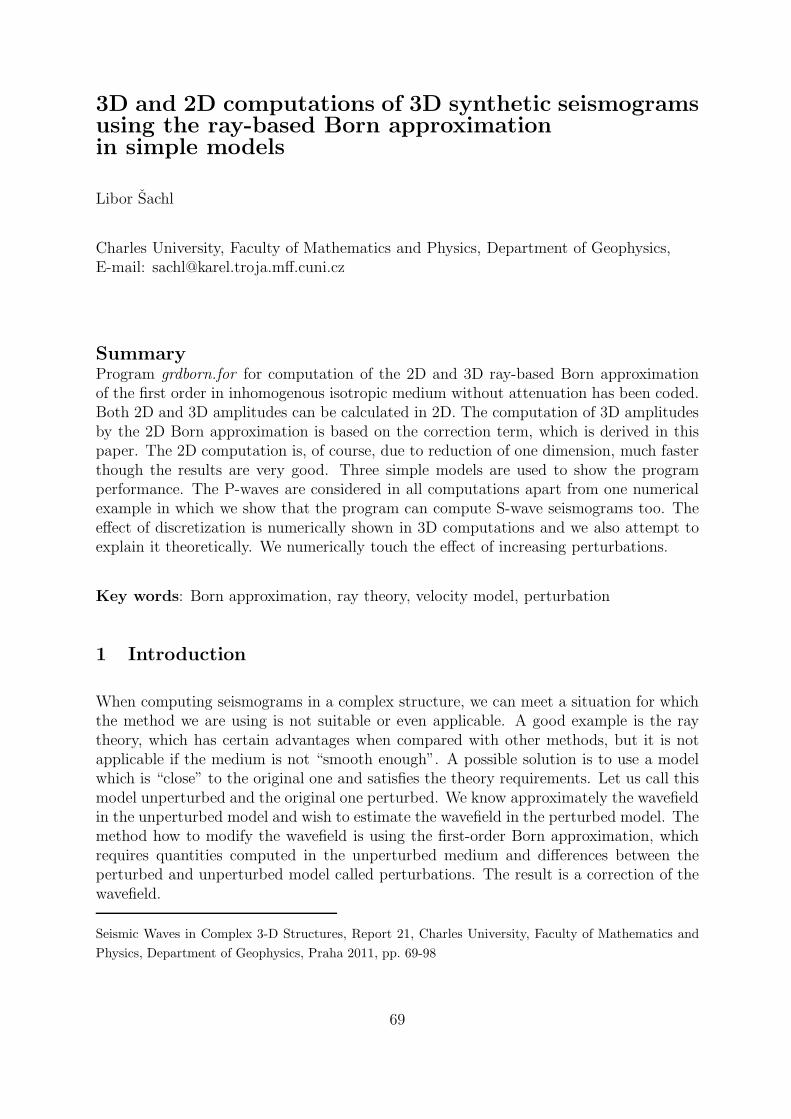
Model 1 has a horizontal interface in the depth of 10 km. The model volume is(0 km, 10 km)× (0 km, 10 km)× (0 km, 20 km). See Figure 1.

Model 2 has an inclined interface with slope 2/5. The model volume is (−5 km, 10 km)×(0 km, 10 km)× (0 km, 20 km). See Figure 2.

Model 3 has a curved interface. The model volume is (−5 km, 15 km)×(0 km, 10 km)×(0 km, 20 km). See Figure 3.

4 Numerical examples of 3D computations of 3D seismograms

In all 3 models, the explosive source is situated at point (2 km, 1 km, 1 km), receiver atpoint (8 km, 9 km, 0 km). The source time function is a Gabor signal with prevailingfrequency 10 Hz, filtered by frequency filter which is nonzero only for frequencies f , 1 Hz< f < 20 Hz. There is a cosine tapering for 1 Hz < f < 2 Hz and 19 Hz < f < 20 Hzwhile for 2 Hz < f < 19 Hz the filter is equal to one. Just P-waves are considered in allnumerical examples except one numerical example focused on S waves.

In the SW3D programs, the following specification of the grid is used: O1, O2, O3

specify the coordinates of the origin of the grid. N1, N2, N3 are the numbers of gridpoints

71

Figure 1: The model volume, the interface and the reflected ray in model 1. The figures of the modelswere created in program GOCAD.

72

Figure 2: The model volume, the interface and the reflected ray in model 2.

73

Figure 3: The model volume, the interface and the reflected rays in model 3.

74

along the x1, x2, x3 coordinate axes, respectively. D1, D2, D3 are the grid intervals inthe directions of the x1, x2, x3 coordinate axes, respectively. We use this notation in thispaper.

4.1 Model 1

4.1.1 Model 1 - grid density

The position of the grid with respect to the horizontal interface is depicted in Figure 4.The unfilled circles represent grid points where perturbations are zero. The interfaceis situated precisely between two grid point planes. The distance between the modelboundary and the nearest grid point plane is equal to the half of the grid interval, becausethe value of any quantity at each grid point represents the value in the block centered atthe grid point with the sides equal to the grid intervals.

s s s s s s s s s

s s s s s s s s s

s s s s s s s s s

c c c c c c c c c

Figure 4: Position of the grid in model 1, which discretize the interface in the best way. Bold line:Model boundary. Thin line: Interface.

For the position of the coordinate axes, refer to Figure 1 in Section 3. The gridinterval is chosen 0.1 km, which is smaller than quarter of wavelength λ = vp/fd ⇒ λ

4=(

14

610

)km = 0.15 km, where we inserted the value of the prevailing frequency of the Gabor

signal fd = 10 Hz and P-wave velocity vp = 6 km/s. The size of the grid is 100×100×100points and covers only the lower part of the model where the perturbation is nonzero inorder to save memory. Figure 5 shows the resulting seismogram. We can see that mainfeatures are captured, but obviously some discrepancies are present. In order to get rid ofthem, we try to densify our grid. First, we densify it twice in the direction of the third axis(For the position of the coordinate axes, refer to Figure 1.). The resulting seismogramdisplayed in Figure 6 is better than the previous one. Second, we try to additionallydensify the grid in the direction of the first axis. It is a bit surprising that it has noimpact on the seismogram. Therefore we step back, use 100 grid points in the directionof the first axis, but apply additional densification in the direction of the third axis. Theseismogram has improved, see Figure 7. There are virtually no differences between theBorn and ray-theory seismogram.

We try to understand the effect of discretization. Let us assume paraxial approxima-tion with the first-order Taylor expansion of travel with respect to the spatial coordinates.The central point is the point of reflection, therefore the derivatives of travel time with

75

3 . 4

3 . 5

3 . 6

3 . 7

3 . 8

T IME

B L A C K . . . B o r n a p p r o x i m a t i o nR E D . . . R a y t h e o r y

r e c 1r e c 13 . 4

3 . 5

3 . 6

3 . 7

3 . 8

T IME


r e c 1r e c 1

Figure 5: Model 1, grid 100 × 100 × 100 grid-points.


3 . 4

3 . 5

3 . 6

3 . 7

3 . 8

T IME


r e c 1r e c 1


76

respect to the first and second coordinate axes are equal to zero and the integral in theBorn approximation in the homogenous model can be simplified to

I0 =

∞∫

0

exp(iωp3x3)dx3 = − 1

iωp3, (8)

where

ω =2πv

λ, p3 = p3 + P3 =

2 cosα

v, (9)

with α being the angle between the slowness vector of the incident wave and the normalto the interface.

Discretisation with the grid interval h affects the integral in the following way:

I1 =∞∑

n=0

h exp

[iωp3

(h

2+ nh

)]= h exp

(iωp3

h

2

)1

1− exp(iωp3h). (10)

Using expressions (8) and (10), we can write

I1I0

− 1 = −iωp3hexp

(iωp3

h2

)

1− exp(iωp3h)− 1,

which readsI1I0

− 1 =ωp3

h2

sin(ωp3h2)− 1. (11)

The expression in (11) is real, therefore the discretisation error influence the amplitudeof the wave but not the phase. We rewrite (11) using (9) as

I1I0

− 1 =2π h

λcosα

sin(2π h

λcosα

) − 1, (12)

which approximately reads

I1I0

− 1 ≈ 1

6

(2π

h

λcosα

)2

. (13)

We compare the numerical results with the theoretical predictions (12) and (13), seeTable 1.

h = D3 [km] Equation (13) [%] Equation (12)[%] Measured [%]0.1 14 16 170.05 3.6 3.7 2.20.025 0.89 0.90 0.90

Table 1: Effect of discretization error on the wave amplitude. The comparison of the theoreticalprediction and the numerical results. D3 is the grid interval in the direction of the third coordinate axis.

Both theoretical predictions (12) and (13) agrees well with numerical modelling incase of the smallest grid interval D3 = 0.025 km. The differences between the theoret-ical predictions and numerical results are observed for D3 = 0.05 km and 0.1 km. Thedifference between the full formula (13) and its first approximation (12) is negligable forD3 = 0.025 km. The difference grows for D3 = 0.05 and is important for D3 = 0.1 km.

77

4.1.2 Model 1 - spurious waves

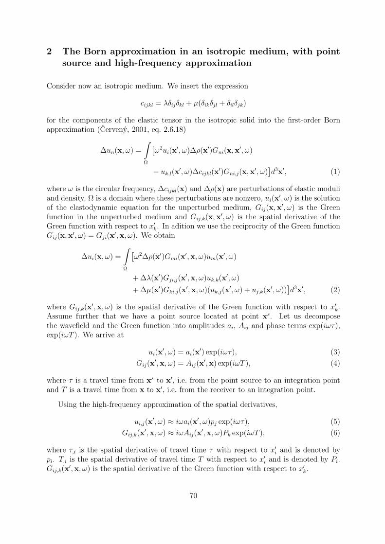
In previous Section 4.1.1, we studied the seismogram in the time window 3.4 − 3.8 sand when we used sufficiently dense grid we did not observe any differences betweenseismograms computed using the Born approximation and the ray theory. However, thedifferences are apparent when we extend our time window from 3.4− 3.8 s to 3.0− 7.2 s,see Figure 8. The differences are caused by interfaces artificially introduced by the grid.Perturbed model has one defined interface. The model is defined within the model volume,but it smoothly continues across the model boundaries. Elastic parameters are not zerooutside the model volume and so model perturbations can be nonzero there, too. In otherwords, model boundaries (side boundaries, bottom and top boundary) are not interfaces.On the contrary, our choice of the grid is equivalent to putting model perturbations zeroelsewhere. In the case of model 1, boundaries of the lower part of the model are treatedas interfaces. From what was said, we expect various types of reflections present in theseismogram, for example the wave reflected from the bottom model interface, as well asdiffractions.

How to distinguish these spurious waves from the right ones? They are sensitive topositions of the grid boundaries. Therefore, if we shift these boundaries, the seismogramsshould change a bit. A good shift is λ

4because the wave has to travel ∆l = 2λ

4= λ

2

longer/shorter in the case of the normal incidence. If the incidence is not normal, thelength of the trajectory changes by ∆l = λ

2cosα where α is the angle between the normal

to the interface and the vector tangent to the ray. We decide to reduce the grid, sothat ∆l < 0 and the shift present in the seismogram should be towards lower times.D1 = D2 = 0.1 km, D3 = 0.025 km, λ

4= 0.15 km, therefore we erase 2 side gridpoint

planes and 8 bottom gridpoint planes, which is equivalent to |∆l| = 0.2 cosα km. Thisvalue is bigger than λ

4for normal incidence, but due to cosine modification for obligue

incidence, a higher value is better than smaller. The seismogram is displayed in Figure 9.

The waves which are shifted in the seismogram should be eliminated. There are atleast two ways how to do it. The first one is safe but computationally expensive. Itconsists in the sufficient extension of the grid. If the grid boundaries (interfaces) are farenough, reflections etc. arrive sufficiently late. The seismogram depicted in Figure 10 iscomputed using the grid which covers the volume of (−10 km, 20 km)×(−10 km, 20 km)×(10 km, 20 km). The grid density is the same as in computation of the seismograms inFigures 7 and 8, but the grid contains 9 times more points. Compare three waves visiblein the seismograms in Figures 8, 9, 10. The first wave is obviously the true wave, becausewe do not see any shift in the seismogram in Figure 9. The second wave and the thirdwave are both shifted in the seismogram in Figure 9, but notice that no shift is presentin the seismogram in Figure 10 in case of the third wave. We enlarge the model in thehorizontal direction, which means that the third wave is the reflection from the bottomof the grid.

One might think, that we can use sparser grid if we are sufficiently far from the sourceand the receiver. If this were true, we would be able to cover big volume with onlya bit more computational effort using varying density grid. Unfortunately we can be

78

3 . 0

4 . 0

5 . 0

6 . 0

7 . 0

T IME


r e c 1r e c 13 . 0

4 . 0

5 . 0

6 . 0

7 . 0

T IME

B L A C K . . . B o r n a p p r o x i m a t i o nR E D . . . B o r n a p p r o x i m a t i o n , s m a l l e r g r i d

r e c 1r e c 1

Figure 8: Model 1, grid 100 × 100 × 400 grid-points, enlarged time window.

Figure 9: Model 1, grid 100 × 100 × 400 grid-points vs grid 96× 96× 392 gridpoints.

3 . 0

4 . 0

5 . 0

6 . 0

7 . 0

T IME


r e c 1r e c 1

Figure 10: Extended model 1, grid 300× 300×400 gridpoints.

79

badly surprised. We try to cover the same volume (−10 km, 20 km)× (−10 km, 20 km)×(10 km, 20 km), but now utilizing combination of two grids. The first grid is sparseand covers the whole volume except the middle part (0 km, 10 km) × (0 km, 10 km) ×(10 km, 20 km). The second grid is dense and covers the middle part. SW3D programswork with regular rectangular grids. We thus have to compose the first grid of tworectangular grids. Grid A is sparse and covers the whole volume, grid B is also sparseand covers the middle part. The first grid is grid A minus grid B. The seismograms fromthe second grid and grid B are correct, but the seismogram from grid A is incorrect, seeFigure 11. It is probable that constructive apart from destructive interference occurred.

The second way how to eliminate a spurious wave is to apply the cosine window on theartificial grid boundaries. 1D cosine window starting at point xs of length L is function

w(x)

= 0 for x < xs

= 12

(1− cos

[π(x−xs)

L

])for x ∈ 〈xs, xs + L〉

= 1 for x > xs + L.

(14)

We introduce the following numbering of the model boundaries, see Table 2.

Axis perpendicular to the boundary Assigned number1-st, negative direction 11-st, positive direction 22-nd, negative direction 32-nd, positive direction 43-rd, negative direction 53-rd, positive direction 6

Table 2: Numbering of the model boundaries

If we apply the cosine window of length L to the 1-st boundary at (x01, •, •), then

cosine window is a function w(x1) defined by (14) with xs = x01 − D1

2. Similarly for other

boundaries.

We apply the cosine windows of the equal length to each grid boundary except the 5-thone, where we model the reflection. Tested lengths are L = 1 km, L = 1.5 km, L = 2 km,L = 2.5 km, L = 3 km The corresponding seismograms are displayed in Figures 12, 13,14, 15, 16.

Remark that amplitudes of the spurious waves decrease and the waves arrive earlier.The values of L = 2.5 km or L = 3 km are obviously too big, the spurious wave arrives soearly that it interferes with the right wave. Another important fact is that the reflectionfrom the bottom grid boundary is very well damped while diffractions from the side gridboundaries are damped worse.

This phenomenon can be explained in a similar way as we derived formula (13). Werewrite the expression (14) for cosine window of length L as

w(x) =1− cos

(π x

L

)

2=

1

2− 1

4exp

(iπ

x

L

)− 1

4exp

(−iπ

x

L

). (15)

80

3 . 0

4 . 0

5 . 0

6 . 0

7 . 0

T IME


r e c 1r e c 13 . 0

4 . 0

5 . 0

6 . 0

7 . 0

T IME


r e c 1r e c 1

Figure 11: Extended model 1, grid 75×75×400gridpoints.

Figure 12: Model 1, grid 100× 100× 400 grid-points, cosine window of length 1 km applied togrid boundaries 1,2,3,4,6 (see Table 2).

The Born approximation with applied cosine window can be reduced to

I1 =

L∫

0

w(x) exp(iωp3x3)dx3 +

∞∫

L

exp(iωp3x3)dx3

=1

2iωp3[exp(iωp3L)− 1]− 1

4(i πL+ iωp3

) [exp(iπ + iωp3L)− 1]

− 1

4(−i π

L+ iωp3

) [exp(−iπ + iωp3L)− 1]− 1

iωp3exp(iωp3L),

which can be rewriten into factorized form

I1 =

[1

4(iωp3 + i π

L

) +1

4(iωp3 − i π

L

) − 1

2iωp3

][1 + exp(iωp3L)] (16)

=12

(πL

)2

iωp3

[(ωp3)2 −

(πL

)2] [1 + exp(iωp3L)] . (17)

81

3 . 0

4 . 0

5 . 0

6 . 0

7 . 0

T IME


r e c 1r e c 13 . 0

4 . 0

5 . 0

6 . 0

7 . 0

T IME


r e c 1r e c 1

Figure 13: Model 1, grid 100× 100× 400 grid-points, cosine window of length 1.5 km applied togrid boundaries 1,2,3,4,6.

Figure 14: Model 1, grid 100× 100× 400 grid-points, cosine window of length 2 km applied togrid boundaries 1,2,3,4,6.

3 . 0

4 . 0

5 . 0

6 . 0

7 . 0

T IME


r e c 1r e c 13 . 0

4 . 0

5 . 0

6 . 0

7 . 0

T IME


r e c 1r e c 1



82

Using expressions (8) and (17) we can express

I1I0

=

(πL

)2(πL

)2 − (ωp3)2

1 + exp(iωp3L)

2. (18)

If we suppose that ωp3L ≫ π, we have

∣∣∣∣I1I0

∣∣∣∣ <(

π

ωp3L

)2

,

and finally, employing (9), ∣∣∣∣I1I0

∣∣∣∣ <(

λ

4L cosα

)2

. (19)

4.1.3 Modified model 1 - applicability of the ray based Born approximation

We shall now study, how well the Born approximation behaves if medium perturbationsincrease. The grid is identical with the one used in the computation of the seismogramshown in Figure 7. Values of the elastic parameters in the lower layer are graduallyincreased to obtain the following perturbations of elastic parameters:

∆vp = 0.1 km/s, ∆vs = 0.1 km/s, ∆ρ = 100kg/m3, (20)

∆vp = 0.5 km/s, ∆vs = 0.5 km/s, ∆ρ = 500kg/m3, (21)

∆vp = 1 km/s, ∆vs = 1 km/s, ∆ρ = 1000kg/m3. (22)

Resulting seismograms are displayed in Figures 17, 18, 19. The scale is chosen to havepractically equal ray-theory seismogram. It is interesting that, though perturbations (20)are 10 times greater than in the computation of the seismogram of Figure 7, the seis-mograms looks still quite well. Discrepancies appear and grow for greater perturbations.It is probably consequence of the nonlinearity of the reflection coefficient, see also Sachl(2011, sec. 3.2, fig. 22).

4.1.4 Model 1 - other types of waves

So far we have tested the algorithm for P-waves. Now we shall focus on other possiblesituations, i.e. incident P wave and scattered S wave (P-S for short), S-P and S-S. Theresulting seismograms corresponding to the first two cases are displayed in Figures 20and 21. Good agreement is observed. In the last case composed purely of S-waves,discrepancies are observed, see Figure 22. Note that vp = 6 km/s, vs = 3 km/s and thus

λs =λp

2. Therefore the grid should be twice denser to be effectively the same as in case

of P-waves. For the grid twice denser in the vertical direction, discrepancies disappear,see Figure 23.

83

3 . 4

3 . 5

3 . 6

3 . 7

3 . 8

T IME


r e c 1r e c 13 . 4

3 . 5

3 . 6

3 . 7

3 . 8

T IME


r e c 1r e c 1

Figure 17: Model 1, grid 100× 100× 400 grid-points, perturbations (20).


3 . 4

3 . 5

3 . 6

3 . 7

3 . 8

T IME


r e c 1r e c 1


84

5 . 2 0

5 . 3 0

5 . 4 0

5 . 5 0

T IME


r e c 1r e c 15 . 0

5 . 1

5 . 2

5 . 3

T IME


r e c 1r e c 1

Figure 20: Model 1, incident P wave, scatteredS wave, grid 100× 100× 400 gridpoints.

Figure 21: Model 1, incident S wave, scatteredP wave, grid 100× 100× 400 gridpoints.

6 . 9

7 . 0

7 . 1

7 . 2

7 . 3

7 . 4

T IME


r e c 1r e c 16 . 9

7 . 0

7 . 1

7 . 2

7 . 3

7 . 4

T IME


r e c 1r e c 1

Figure 22: Model 1, incident S wave, scatteredS wave, grid 100× 100× 400 gridpoints.

Figure 23: Model 1, incident S wave, scatteredS wave, grid 100× 100× 800 gridpoints.

85

4.2 Model 2

4.2.1 Model 2 - grid

We choose N2 = 100 for the computations in this 3D model. This number of gridpointsalong the second coordinate axis is equal to the value used in Section 4.1. For the positionof the coordinate axes, refer to Figure 2 in Section 3. Slope of the inclined interface is 2

5.

We choose the grid which fits the shape and position of the interface, i.e. the interfacelies between two grid point planes, see Figure 24. We thus take

D1 =5

2D3 (23)

We set N3 = 400. The interface begins in the depth 6 km, so that D3 = 0.034956 km ≈20−6

N3+0.5km, therefore D1 ≈ 0.087391 km and N1 = 171 ≈ 15 km

D1

.

s s s s

s s s s

s s s s

s s s saaaaaaaaaaaaaaaaaaaaaa

Figure 24: Grid which fits the shape and position of the interface in model 2. Cross section in x1 − x3

plane. Bold line: Model boundary. Thin line: Interface.

Using this configuration, we calculate the seismogram displayed in Figure 25. TheBorn and ray-theory seismograms agree very well, despite the fact that grid interval D3

is bigger than in the computation of the seismogram in Figure 5 and discretization ofthe interface is worse too. Indeed, in model 1, discretization is h = D3 = 0.025 km. Inmodel 2, h is equal to the altitude in the right triangle with legs D1, D3,

h =D1D3√D2

1 +D23

, (24)

inserting (23) we obtain

h =5√29

D3 ≈ 0.0232 km. (25)

4.2.2 Model 2 - spurious waves

Spurious waves are revealed in the same way as in model 1, see Figure 26. They aresuppressed by using cosine windows of lengths 0.5 km, 1 km and 1.5 km respectively.The results are depicted in Figures 27, 28, 29.

86

3 . 1

3 . 2

3 . 3

3 . 4

3 . 5

3 . 6

T IME


r e c 1r e c 12 . 8

3 . 8

4 . 8

5 . 8

6 . 8

7 . 8

T IME


r e c 1r e c 1

Figure 25: Model 2, grid 171× 100× 400 grid-points.

Figure 26: Model 2, grid 171× 100× 400 grid-points, enlarged time window.

4.3 Model 3

For the position of the coordinate axes, refer to Figure 3 in Section 3. The grid of300× 100× 800 points is chosen. The grid intervals are D1 = 0.066667 km, D2 = 0.1 kmand D3 = 0.025 km. The grid interval in the direction of the third axis is the same as inthe computation of the seismogram in Figure 7. Shape of the interface does not dependon x2, therefore 100 grid points in the direction of the second coordinate axis would seemenough. The seismogram computed using this grid is displayed in Figure 30. We cansee differences between the Born and ray-theory seismogram in Figure 30, therefore wecompute the Born approximation with more precise grid values of elastic parameters. Wediscretize the density, P-wave and S-wave velocity on the grid twice denser in the directionof the first and third axes. The quantities are then averaged to the above described grid.The density is averaged by geometrical mean, which corresponds to the conservation ofmass inside the volume determined by the averaged grid cell. The P-wave and S-wavevelocities are averaged by harmonic mean, which corresponds to the conservation of traveltime inside the volume determined by the averaged grid cell. We obtain the seismogramin Figure 31. We see improvement in the first wave, but more important effect is thereduction of oscillations visible on the previous seismogram around 3.72 s, i.e. after thesecond wave. We further try to densify used grid. Interface is quite complicated in planex1-x3 and so we consider that discretization in the direction of the 1-st axis could beinsufficient. Therefore we use grid with 600 × 100 × 800 grid points, i.e. we densify it

87

2 . 8

3 . 8

4 . 8

5 . 8

6 . 8

7 . 8

T IME


r e c 1r e c 12 . 8

3 . 8

4 . 8

5 . 8

6 . 8

7 . 8

T IME


r e c 1r e c 1



2 . 8

3 . 8

4 . 8

5 . 8

6 . 8

7 . 8

T IME


r e c 1r e c 13 . 0

3 . 1

3 . 2

3 . 3

3 . 4

3 . 5

3 . 6

3 . 7

3 . 8

T IME


r e c 1r e c 1


Figure 30: Model 3, grid 300× 100× 800 grid-points.

88

3 . 0

3 . 1

3 . 2

3 . 3

3 . 4

3 . 5

3 . 6

3 . 7

3 . 8

T IME


r e c 1r e c 13 . 0

3 . 1

3 . 2

3 . 3

3 . 4

3 . 5

3 . 6

3 . 7

3 . 8

T IME


r e c 1r e c 1

Figure 31: Model 3, grid 300× 100× 800 grid-points, averaged elastic parameters.

Figure 32: Model 3, grid 600× 100× 800 grid-points, averaged elastic parameters.

twice in the direction of the 1-st axis. The elastic parameters are again computed onthe grid twice denser in the direction of the first and third axes and then averaged asin the previous example. The resulting seismogram, see Figure 32, is satisfactory forlower arrival time, say until 3.4 s. But there is evidently something wrong with the waveswhich arrive later. This discrepancy is radically improved after applying cosine windowof length L = 1.5 km, see Figure 33. Our opinion is that it is caused by diffracted wavesproduced by introduction of the grid needed for the numerical calculation. More precisely,we claim that these spurious waves come from the intersection between the grid boundaryperpendicular to the second coordinate axis and the interface. To prove it see the nextcomputation.

Grid contains 666×100×3200 gridpoints. The elastic parameters are discretized in thesame grid. We apply cosine window only in the direction of the second coordinate axis.We acquire Figure 34, which is similar to Figure 33. The agreement between the Bornand ray-theory seismograms is even a bit better. On the other hand, almost 4.5 timesmore grid points are used (though elastic parameters are not computed in the denser gridand averaged). Notice also Figure 35 where we shift the grid boundary perpendicular tothe second coordinate axis, i.e. we made the grid smaller in the direction of the secondcoordinate axis. The shift is equal to 0.2 km, i.e. approximately λ

4as in similar previous

situations. The first wave in the seismogram is unaffected, while the second wavegroup isshifted. The wavegroup is distorted, which means that the wavegroup is a superpositionof two waves. One wave shifts and another one does not shift. The reflected wave is mixedwith the numerically diffracted wave.

89

3 . 0

3 . 1

3 . 2

3 . 3

3 . 4

3 . 5

3 . 6

3 . 7

3 . 8

T IME


r e c 1r e c 13 . 0

3 . 1

3 . 2

3 . 3

3 . 4

3 . 5

3 . 6

3 . 7

3 . 8

T IME


r e c 1r e c 1

Figure 33: Model 3, grid 600× 100× 800 grid-points, averaged elastic parameters, cosine win-dow of length 1.5 km applied to grid boundaries1,2,3,4,6.

Figure 34: Model 3, grid 666× 100× 3200 grid-points, cosine window of length 1.5 km applied togrid boundaries 3,4.

3 . 0

3 . 1

3 . 2

3 . 3

3 . 4

3 . 5

3 . 6

3 . 7

3 . 8

T IME


r e c 1r e c 1

Figure 35: Model 3, grid 666× 100× 3200 grid-points vs grid 666× 96× 3200 gridpoints.

90

5 Theory of 2D computations of 3D seismograms

If the source and receiver are situated in a symmetry plane of a 2D model, we can computethe Born approximation numerically in 2D slice and perform the remaining one dimen-sional integration in the direction perpendicular to the slice analytically (Cerveny & Cop-poli, 1992). Of course, we do not know values of the quantities present in the Bornapproximation there. We use paraxial approximation:

ui(x) = ai(x0) exp

[iω

(τ0 + τ,i∆xi +

1

2τ,ij∆xi∆xj

)], (26)

where x0 is a point in the slice, ∆x = x − x0 and ∆x is perpendicular to the slice,τ0 = τ(x0), τ,22 = τ,22(x0). Let us introduce the coordinate system in which all points inthe slice have the second coordinate equal to zero. Than x0 = (x1, 0, x3), ∆x = (0, x2, 0)and (26) has the form

ui(x) = ai(x0) exp

[iω

(τ0 +

1

2τ,22x

22

)], (27)

Notice that the first-order spatial derivative of travel time with respect to x2 is not present,because it is equal to zero. Travel time is an even function of x2. Derivative of an evenfunction is an odd function and an odd function is zero for x2 = 0. In fact, also thethird-order spatial derivative of travel time with respect to x2 is equal to zero since thesecond-order spatial derivative of travel time with respect to x2 is an even function. Thespatial derivatives in the high-frequency approximation read

ui,j(x) = iω(τ0,j + δj2τ,22x2)ai(x0) exp

[iω

(τ0 +

1

2τ,22x

22

)], (28)

where we neglected 12τ,22jx

22 = 1

2(δj1τ,221 + δj3τ,223)x

22 (see discussion after formula (43)).

Similarly for the Green function.

Gij(x) = Aij(x0) exp

[iω

(T0 +

1

2T,22x

22

)], (29)

Gij,k(x) = iω(T0,k + δk2T,22x2)Aij(x0) exp

[iω

(T0 +

1

2T,22x

22

)]. (30)

Recall the Born approximation (2) in an isotropic medium and decompose it into threeparts

IA = ω2

∫

Ω

∆ρ(x′)Gmi(x′,x, ω)um(x

′, ω)d3x′, (31)

IB =

∫

Ω

∆λ(x′)Gji,j(x′,x, ω)uk,k(x

′, ω)d3x′, (32)

IC =

∫

Ω

∆µ(x′)Gki,j(x′,x, ω)(uk,j(x

′, ω) + uj,k(x′, ω))d3x′. (33)

91

We insert (27) and (29) into the first part of the Born approximation (31) with notationS for the slice and obtain

I1 = ω2

∫

S

∆ρAjiaj exp[iω(τ0 + T0)]

∞∫

−∞

exp[iω

2(τ,22 + T,22)x

22

]dx2

dx1dx3, (34)

Integral over slice S is evaluated numerically, we focus on the integral in brackets. We callthis integral Icor1. We introduce small imaginary part of the derivatives of travel times,then we have

Icor1 =

∞∫

−∞

exp[i(ω2(τ,22 + T,22) + iǫ

)x22

]dx2 =

∞∫

−∞

exp[−(ǫ− iA)x2

2

]dx2, (35)

where A = ω2(τ,22+T,22), ǫ > 0, ǫ ≪ 1. We employ the expression for integral of a complex

Gaussian∞∫

−∞

exp(−pt2)dt =

√π

p, ∀p ∈ C : Re(p) > 0 (36)

to obtain

Icor1 =

√π

ǫ− iA≈

√π

−iA=

√2π

A

1

1− i=

√π

ω(τ,22 + T,22)(1 + i). (37)

The second part of the Born approximation (32) is more complicated due to spatialderivatives. Using (27), (28), (29) and (30)

I2 =

∫

S

∆λAjiP0jakp0k exp[iω(τ0 + T0)]

∞∫

−∞

exp[iω

2(τ,22 + T,22)x

22

]dx2

dx1dx3 (38)

+

∫

S

∆λAjiP0ja2τ,22 exp[iω(τ0 + T0)]

∞∫

−∞

x2 exp[iω

2(τ,22 + T,22)x

22

]dx2

dx1dx3

(39)

+

∫

S

∆λA2iT,22akp0k exp[iω(τ0 + T0)]

∞∫

−∞

x2 exp[iω

2(τ,22 + T,22)x

22

]dx2

dx1dx3

(40)

+

∫

S

∆λA2iT,22a2τ,22 exp[iω(τ0 + T0)]

∞∫

−∞

x22 exp

[iω

2(τ,22 + T,22)x

22

]dx2

dx1dx3,

(41)

where P0j = T0,j and p0k = τ0,k. Integrals (39) and (40) are equal to zero because inparentheses we integrate odd function over symmetrical interval. Integral in parentheses

92

in (38) is equal to (37). To compute integral in parentheses in (41) we use formula

∞∫

−∞

t2k exp(−pt2)dt =1.3 . . . (2k − 1)

(2p)k

√π

p, ∀p ∈ C : Re(p) > 0, k = 1, 2, . . . (42)

and obtain

Icor2 ≈√π

2(−iA)3/2= −

√π

2A3

1

1 + i= −

√π

ω3(τ,22 + T,22)3(1− i). (43)

Comparing (37) and (43) we see that

Icor2 ≈Icor1ω

, (44)

therefore in the high-frequency approximation we can neglect (41) and only (38) remains.In other words we can neglect corrections δj2τ,22x2 and δk2T,22x2 in (28) and (30). Similarlyusing (42) can be shown that it is possible to neglect terms 1

2τ,22jx

22 and 1

2T,22jx

22, as we

did when writing (28) and (30).

The third part of the Born approximation (33) has similar structure as the secondpart (32). Therefore we can compute the Born approximation on 2D grid in the sameway as we did on 3D grid, the only modification is the multiplication of the integrand inthe Born integral by term Icor1:

∆ui(x, ω) =

∫

S

√π

ω(τ,22 + T,22)(1 + i)

[ω2∆ρ(x′, ω)Gmi(x

′,x, ω)um(x′, ω)

+ ∆λ(x′, ω)Gji,j(x′,x, ω)uk,k(x

′, ω)

+ ∆µ(x′, ω)Gki,j(x′,x, ω)(uk,j(x

′, ω) + uj,k(x′, ω))

]d3x′. (45)

6 Numerical examples of 2D computations of 3D seismograms

The models 1,2,3 are exactly the same as the ones used in the 3D computations of Section 4and are described in Section 3, but the source and the receiver positions are different. Wemoved the source and the receiver into the symmetry plane. Namely explosive source isat point (1.5 km,0 km,1 km) and the receiver at point (8.5 km,0 km,0 km).

6.1 Model 1

Experienced from the computations in the 3D version of model 1, we directly start withthe grid 100 × 400 points big. The obtained seismogram displayed in Figure 36 shows agood agreement with the reference solution. It is interesting to see how important is thecorrection (37). The seismogram in Figure 37 was computed without this correction. Itwas necessary to use 100 times smaller magnification to visualize it.

93

3 . 2

3 . 3

3 . 4

3 . 5

3 . 6

T IME


r e c 1r e c 13 . 2

3 . 3

3 . 4

3 . 5

3 . 6

T IME


r e c 1r e c 1

Figure 36: Model 1, 2D computation, grid 100×400 gridpoints.

Figure 37: Model 1, 2D computation, grid 100×400 gridpoints, without correction (37), 100 timessmaller magnification.

6.2 Model 2

According to the grid used in the computation of the seismogram in Figure 25, we firstlyselect grid with 171× 400 points. Resulting seismogram displayed in Figure 38 is slightlyless accurate than the seismogram in Figure 25. For the denser grid with 343×800 pointswe get excellent seismogram in Figure 39.

2D computations have undoubtedly one advantage compared to 3D computations.They are much faster. We used 100 times less points in model 2. Therefore one caneasily experiment and get quick results. As an example, we try to shift the whole grid of171 × 400 points downwards. The shift is smaller than D3

2but it is close to this value.

Figure 40 shows the same seismograms as in Figure 38, but they are shifted against eachother. That is correct. The interface is discretized between two grid point planes. We shiftthese planes downwards, so that the Born approximation shifts the interface downwardsand the wave therefore arrives later.

The second experiment shows what happens if gridpoints lie exactly on the interface.It is obviously not a good choice, because one might expect seismogram shifts as in theprevious experiment and in addition rounding error can make the interface nonplanar.The chosen grid coveres the part of the model with vertical coordinate bigger than 6 andit was quite dense, 375× 875 grid points. Despite this fact the seismogram in Figure 41is much worse than the seismograms computed with more suitable grids.

94

2 . 9

3 . 0

3 . 1

3 . 2

3 . 3

T IME


r e c 1r e c 12 . 9

3 . 0

3 . 1

3 . 2

3 . 3

T IME


r e c 1r e c 1



2 . 9

3 . 0

3 . 1

3 . 2

3 . 3

T IME


r e c 1r e c 12 . 9

3 . 0

3 . 1

3 . 2

3 . 3

T IME


r e c 1r e c 1

Figure 40: Model 2, 2D computation, grid 171×400 gridpoints, wrong discretization cause shift ofthe interface.

Figure 41: Model 2, 2D computation, grid375× 875 gridpoints, grid rectangles centered onthe interface.

95

6.3 Model 3

Motivated by the computation of seismogram in Figure 34 in Section 4.3, we choose gridcontaining 600×3200 grid points. The calculated Born seismogram corresponds very wellto the ray-theory seismogram, see Figure 42.

In 2D computation, there is no grid boundary perpendicular to the second coordinateaxis thanks to the used numerical method (analytical integration in the direction of thesecond coordinate axis). Remember that using analogous grid in 3D computation inSection 4.3, we did not obtain agreement between the Born and ray-theory seismogramsuntil we applied cosine window of length of L = 1.5 km in the direction of the secondaxis.

We also try grid, which contains 600× 800 gridpoints, see Figure 43. It is interestingthat the first wave is already well resolved using this grid, while there are apparent wrongoscillations on the second wave.

2 . 8

2 . 9

3 . 0

3 . 1

3 . 2

3 . 3

3 . 4

3 . 5

3 . 6

T IME


r e c 1r e c 12 . 8

2 . 9

3 . 0

3 . 1

3 . 2

3 . 3

3 . 4

3 . 5

3 . 6

T IME


r e c 1r e c 1



96

7 Concluding remarks

We tested the ray-based first-order Born approximation in homogenous background mod-els. If the Born integral (2) is evaluated numerically using computational grid, we shouldexpect spurious waves introduced by the finite size of the grid. These waves are eitherreflections or diffractions from the grid boundaries. This effect was observed and sup-pressed applying the cosine window of the appropriate length to the integrand of theBorn integral, see Sections 4.1.2, 4.2.2 and 4.3. The effect of the cosine window on thespurious wave reflected from the grid boundary depends on the angle of incidence con-siderably. For large angle of incidence, application of the cosine window is problematic.This phenomenon was numerically observed and theoretically described in formula (19).Another possibility how to get rid of these spurious waves is to enlarge the computationalvolume, which is safe but numerically expensive method. The discretization of the Bornintegral brings also errors in the amplitude of the wave. Formulas (11) and (12) describethis effect.

The Born approximation is suitable for small differences in elastic parameters betweenthe perturbed and unperturbed model. In model 1, see Section 3, we touched the problemof growing perturbations. The elastic parameters in the background were vp = 6 km/s,vs = 3 km/s and ρ = 2000 kg/m3. If perturbations of all elastic parameters were equalto (20) the seismogram was modelled correctly. For perturbations equal to (21) discrep-ancies were observed and they grow and are significant for perturbations equal to (22).

If the interface is shifted due to wrong discretization, the seismogram is shifted intime, see Figure 40.

We derived the form of the Born approximation usable if the source and receiver aresituated in a symmetry plane of a 2D model. The integral is two dimensional in theresulting formula (45). The formula works with 3D amplitudes of the incident wavefieldand of the Green function. The formula was numerically tested in Sections 6.1, 6.2 and6.3 with very good results.

Acknowledgements

First of all I would like to thank Ludek Klimes, who greatly helped me with the workwhich led to this paper. I would also like to thank Vaclav Bucha who helped me with thefigures of models in Section 3.

The research has been supported by the Grant Agency of the Czech Republic undercontract P210/10/0736, by the Ministry of Education of the Czech Republic within re-search project MSM0021620860, and by the members of the consortium “Seismic Wavesin Complex 3-D Structures” (see “http://sw3d.cz”).

97

References

Cerveny, V. (2001): Seismic ray theory, Cambridge Univ. Press., Cambridge.

Cerveny V. & Coppoli A. D. M. (1992): Ray-Born synthetic seismograms for complexstructures containing scatterers. In: Journal of seismic exploration 1, 191-206.

Sachl, L. (2011): 2D computations of 3D synthetic seismograms using the ray based Bornapproximation in heterogenous background model P1. In: Seismic Waves in Complex

3–D Structures, Report 21, pp. 99-114, Dep. Geophys., Charles Univ., Prague.

98

3d and 2d computations of 3d synthetic seismograms using

Documents