seismic attenuation due to wave-induced flowsantos/research/fracture...seismic attenuation due to...

$: Seismic attenuation due to wave-induced flowsantos/research/fracture...Seismic attenuation due to wave-induced flow S. R. Pride Earth Sciences Division, Lawrence Berkeley National$
Seismic attenuation due to wave-induced flow

S. R. PrideEarth Sciences Division, Lawrence Berkeley National Laboratory, Berkeley, California, USA

J. G. BerrymanUniversity of California, Lawrence Livermore National Laboratory, Livermore, California, USA

J. M. HarrisDepartment of Geophysics, Stanford University, Stanford, California, USA

Received 19 June 2003; revised 9 October 2003; accepted 23 October 2003; published 14 January 2004.

[1] Three P wave attenuation models for sedimentary rocks are given a unifiedtheoretical treatment. Two of the models concern wave-induced flow due toheterogeneity in the elastic moduli at ‘‘mesoscopic’’ scales (scales greater than grainsizes but smaller than wavelengths). In the first model, the heterogeneity is due tolithological variations (e.g., mixtures of sands and clays) with a single fluid saturatingall the pores. In the second model, a single uniform lithology is saturated in mesoscopic‘‘patches’’ by two immiscible fluids (e.g., air and water). In the third model, theheterogeneity is at ‘‘microscopic’’ grain scales (broken grain contacts and/or microcracksin the grains), and the associated fluid response corresponds to ‘‘squirt flow.’’ Themodel of squirt flow derived here reduces to proper limits as any of the fluid bulkmodulus, crack porosity, and/or frequency is reduced to zero. It is shown that squirt flow isincapable of explaining the measured level of loss (10�2 < Q�1 < 10�1) within the seismicband of frequencies (1–104 Hz); however, either of the two mesoscopic scale modelseasily produces enough attenuation to explain the field data. INDEX TERMS: 0935 Exploration

Geophysics: Seismic methods (3025); 5102 Physical Properties of Rocks: Acoustic properties; 5114 Physical

Properties of Rocks: Permeability and porosity; 5144 Physical Properties of Rocks: Wave attenuation;

KEYWORDS: seismic attenuation, poroelasticity, seismic dispersion

Citation: Pride, S. R., J. G. Berryman, and J. M. Harris (2004), Seismic attenuation due to wave-induced flow, J. Geophys. Res., 109,

B01201, doi:10.1029/2003JB002639.

1. Introduction

[2] The physics controlling the intrinsic seismic attenua-tion of sedimentary rock throughout the seismic band offrequencies (say 1 to 104 Hz) is still not entirely understood.In particular, seismic data from sedimentary regions oftenexhibits more intrinsic attenuation than can be explainedusing existing theoretical models. The principal goal of thispaper is to provide models that can help explain the levelsof loss determined from seismograms.[3] Intrinsic loss is often quantified using the inverse

quality factor Q�1 which represents the fraction of waveenergy lost to heat in each wave period. For seismictransmission experiments (earthquake recordings, VSP,cross-well tomography, sonic logs), the total attenuationinferred from the seismograms can be decomposed asQtotal

�1 = Qscat�1 + Q�1 where both the scattering and intrinsic

contributions are necessarily positive. In transmissionexperiments, multiple scattering transfers energy from thecoherent first-arrival pulse into the coda and into directionsthat will not be recorded on the seismogram, and is thus

responsible for the effective ‘‘scattering attenuation’’ Qscat�1 .

Techniques have been developed that attempt to separate theintrinsic loss from the scattering loss in transmission experi-ments [e.g., Wu and Aki, 1988; Sato and Fehler, 1998]. Inseismic reflection experiments, backscattered energy fromthe random heterogeneity can sometimes act to enhance theamplitude of the primary reflections. At the present time,techniques that can reliably separate the total inferred loss ofa reflection experiment into scattering and intrinsic portionsare generally not available.[4] Cross-well experiments in horizontally stratified sedi-

ments produce negligible amounts of scattering loss so thatessentially all apparent loss (except for easily correctedspherical spreading) is attributable to intrinsic attenuation.Quan and Harris [1997] use tomography to invert theamplitudes of cross-well P wave first arrivals to obtain theQ�1 for the layers of a stratified sequence of shaly sandstonesand limestones (depths ranging from 500 to 900 m). Thecenter frequency of their measurements is roughly 1750 Hzand they find that 10�2 < Q�1 < 10�1 for all the layers in thesequence. Sams et al. [1997] also measure the intrinsic loss ina stratified sequence of water-saturated sandstones, siltstonesand limestones (depths ranging from 50 to 250 m) using

JOURNAL OF GEOPHYSICAL RESEARCH, VOL. 109, B01201, doi:10.1029/2003JB002639, 2004

Copyright 2004 by the American Geophysical Union.0148-0227/04/2003JB002639$09.00

B01201 1 of 19

VSP (30–280 Hz), cross-well (200–2300 Hz), sonic logs(8–24 kHz), and ultrasonic laboratory (500–900 kHz)measurements. Sams et al. [1997] calculate (withsome inevitable uncertainty) that in the VSP experiments,Q�1/Qscat

�1 � 4, while in the sonic experiments, Q�1/Qscat�1 �

19; that is, for this sequence of sediments, the intrinsic lossdominates the scattering loss at all frequencies. Sams et al.[1997] also find 10�2 < Q�1 < 10�1 across the seismic band.[5] It will be demonstrated here that wave-induced fluid

flow generates enough heat to explain these measured levelsof intrinsic attenuation. Other attenuation mechanisms neednot be considered since they are likely contributing muchsmaller percentages to the overall observed attenuation. Theinduced flow occurs at many different spatial scales that canbroadly be categorized as ‘‘macroscopic,’’ ‘‘mesoscopic,’’and ‘‘microscopic.’’[6] The macroscopic flow is the wavelength-scale equil-

ibration occurring between the peaks and troughs of aP wave. This mechanism was first treated by Biot [1956a,1956b] and is often simply called ‘‘Biot loss.’’ However, theflow at such macroscales drastically underestimates themeasured loss in the seismic band (by as much as 5 ordersof magnitude). Two possible alternatives to Biot loss weretherefore proposed in the mid-1970s.[7] First, Mavko and Nur [1975, 1979], Budiansky and

O’Connell [1976], and O’Connell and Budiansky [1977]proposed a microscopic mechanism due to microcracks inthe grains and/or broken grain contacts. When a seismicwave squeezes a rock having such grain-scale damage, thecracks respond with a greater fluid pressure than the mainpore space resulting in a flow from crack to pore that Mavkoand Nur [1975] named ‘‘squirt flow’’. Dvorkin et al. [1995]have also presented a squirt flow model applicable to liquid-saturated rocks. Although squirt flow seems capable ofexplaining much of the measured attenuation in the labora-tory at ultrasonic frequencies and may also turn out to beimportant for propagation in ocean sediments at ultrasonicfrequencies [Williams et al., 2002], we show here that thismechanism cannot explain the attenuation in the seismicband.[8] Second, White [1975] and White et al. [1975] mod-

eled the wave-induced flow created by mesoscopic-scaleheterogeneity. Mesoscopic length scales are those largerthan grain sizes but smaller than wavelengths. Heterogene-ity across these scales may be due to lithological variationsor to patches of different immiscible fluids. When a com-pressional wave squeezes a material containing mesoscopicheterogeneity, the effect is similar to squirt with the morecompliant portions of the material responding with a greaterfluid pressure than the stiffer portions. There is a subsequentflow of fluid capable of generating significant loss in theseismic band.[9] White [1975] considered the flow in a concentric

porous sphere model in which the inner sphere is saturatedby one fluid type (say gas), the outer shell is saturated byanother fluid type (say liquid), and the porous frame proper-ties are everywhere uniform. This is the first so-called‘‘patchy saturation’’ model. White had the insight to use theBiot [1956a, 1956b] theory as the local model for the meso-scopic flow between the spheres. Dutta and Ode [1979a,1979b] and Dutta and Seriff [1979] went on to make severalimportant corrections to the initial White [1975] model, add-

ing to our understanding of the low-frequency and high-frequency limits. White’s [1975] prediction of enhancedattenuation in the presence of even small volume fractionsof gas phase has been experimentally confirmed [e.g.,Murphy, 1982, 1984; Cadoret et al., 1998].[10] White et al. [1975] considered the wave-induced

flow between the mesoscopic-scale layers in a sedimentarybasin. Here the mesoscopic heterogeneity is in the frameproperties of the porous rocks with a single fluid saturatingall layers. Again, Biot theory was used as the local modelfor the mesoscopic flow. A host of theoretical refinementshave subsequently been added to White’s initial model ofmesoscopic flow in finely layered media [e.g., Norris, 1993;Gurevich and Lopatnikov, 1995; Gelinsky and Shapiro,1997].[11] More recent work by Johnson [2001] has treated

wave-induced mesoscopic flow due to patchy saturationwithout placing restrictions on the patch geometries. Thepresent study also seeks to model the wave-induced flowfor arbitrary mesoscopic geometry due either to litholog-ical variations or to patchy saturation, albeit under therestriction that only two porous phases are mixed togetherin each averaging volume. Furthermore, our same formal-ism is shown to produce new exact results at both low andhigh frequencies for the Dvorkin et al. [1995] squirt flowmodel.[12] In section 2, we review the recent theory of Pride

and Berryman [2003a, 2003b] treating the mesoscopicloss created by lithological patches having, for example,different degrees of consolidation. This so-called ‘‘double-porosity’’ model provides the theoretical framework thatwill be used throughout. In section 3, we reanalyze thepatchy saturation model of Johnson [2001] and demon-strate numerically that our double-porosity approach tothe problem is asymptotically identical to Johnson’s resultin the limits of low and high frequencies (both analysesare exact for the model in the two limits). In section 4,we provide a new analysis of the Dvorkin et al. [1995]squirt flow model that is numerically compared to theapproximate analysis of Dvorkin et al. [1995]. Finally, inthe concluding section 5, we summarize what has beenlearned from these models.

2. Review of the Double-Porosity Theory

[13] In this theory, the mesoscopic heterogeneity is mod-eled as a mixture of two porous phases saturated by a singlefluid.[14] Various scenarios can be envisioned for how two

porous phases might come to reside within a single geo-logical sample. For example, even within an apparentlyuniform sandstone formation, there can remain a smallvolume fraction of less consolidated (even noncemented)sand grains. This is because diagenesis is a transport processsensitive to even subtle heterogeneity in the initial grainpack resulting in spatially variable mineral deposition [e.g.,Thompson et al., 1987] and, supposedly, in spatially vari-able elastic moduli. Alternatively, the two phases mightcorrespond to interwoven lenses of detrital sands and clays;however, any associated anisotropy in the deviatoric seismicresponse will not be modeled in the present paper. Jointedrock is also reasonably modeled as a double-porosity

B01201 PRIDE ET AL: WAVE-INDUCED FLOW LOSSES

2 of 19

B01201

material. The joints or macroscopic fractures are typicallymore compressible and have a higher intrinsic permeabilitythan the background host rock they reside within.

2.1. Local Governing Equations

[15] Each porous phase is locally modeled as a porouscontinuum and obeys the laws of poroelasticity [e.g., Biot,1962]

r � TDi �rpci ¼ r�ui þ rf _Qi; ð1Þ

Qi ¼ � ki

hrpfi þ rf �ui� �

; ð2Þ

r � _ui

r �Qi

24

35 ¼ � 1

Kdi

1 �ai

�ai ai=Bi

24

35 _pci

_pfi

24

35; ð3Þ

TDi ¼ Gi rui þruTi � 2

3r � ui I

� �; ð4Þ

where the index i represents the two phases (i = 1, 2). Theresponse fields in these equations are themselves localvolume averages taken over a scale larger than the grainsizes but smaller than the mesoscopic extent of either phase.The local fields are: ui, the average displacement of theframework of grains;Qi, the Darcy filtration velocity; pfi, thefluid pressure; pci, the confining pressure (total averagepressure); andTi

D, the deviatoric (or shear) stress tensor. In thelinear theory of interest here, the overdots on these fieldsdenote a partial time derivative. In the local Darcy law (2), h isthe fluid viscosity and the permeability ki is a linear timeconvolution operator whose Fourier transform ki (w) is calledthe ‘‘dynamic permeability’’ and can be modeled using thetheory of Johnson et al. [1987] (see Appendix A).[16] In the local compressibility law (3), Ki

d is the drainedbulk modulus of phase i (confining pressure change dividedby sample dilatation under conditions where the fluid pres-sure does not change), Bi is Skempton’s [1954] coefficient ofphase i (fluid pressure change divided by confining pressurechange for a sealed sample), and ai is the Biot and Willis[1957] coefficient of phase i defined as

ai ¼ ð1� Kdi =K

ui Þ=Bi; ð5Þ

where Kiu is the undrained bulk modulus (confining pressure

change divided by sample dilatation for a sealed sample). Inthe present work, no restrictions to single-mineral isotropicgrains will be made. Finally, in the deviatoric constitutivelaw (4),Gi is the shearmodulus of the framework of grains. Atthe local level, all these poroelastic constants are taken to bereal constants. In Appendix Awe give the Gassmann [1951]fluid substitution relations that allowBi andai to be expressedin terms of the porosity fi, the fluid and solid bulk moduli Kf

and Ks, and the drained modulus Kid.

2.2. Double-Porosity Governing Equations

[17] In the double-porosity theory, the goal is to deter-mine the average fluid response in each of the porousphases in addition to the average displacement of the solidgrains [Berryman and Wang, 1995]. The averages are takenover regions large enough to significantly represent bothporous phases, but smaller than wavelengths. Assuming an

e�iwt time dependence, Pride and Berryman [2003a] havevolume averaged the local laws (1)–(4) to obtain themacroscopic ‘‘double-porosity’’ governing equations inthe form

r � TD �rPc ¼ �iw rvþ rf q1 þ rf q2� �

; ð6Þ

q1

q2

24

35 ¼ � 1

h

k11 k12

k12 k22

24

35 �

rpf 1 � iwrf v

rpf 2 � iwrf v

24

35; ð7Þ

r � v

r � q1

r � q2

266664

377775 ¼ iw

a11 a12 a13

a12 a22 a23

a13 a23 a33

266664

377775 �

Pc

pf 1

pf 2

266664

377775þ iw

0

zint

�zint

266664

377775; ð8Þ

�iwzint ¼ g wð Þ pf 1 � pf 2

� �; ð9Þ

�iwTD ¼ G wð Þ � iwg wð Þ½ rvþ rvð ÞT� 2

3r � v I

� �: ð10Þ

The macroscopic fields are v, the average particle velocityof the solid grains throughout an averaging volume of thecomposite; qi, the average Darcy flux across phase i; Pc,the average total pressure in the averaging volume; TD, theaverage deviatoric stress tensor; �pfi, the average fluidpressure within phase i; and �iwzint, the average rate atwhich fluid volume is being transferred from phase 1 intophase 2 as normalized by the total volume of the averagingregion. The dimensionless increment zint represents the‘‘mesoscopic flow.’’[18] Equation (7) is the generalized Darcy law allowing

for fluid cross coupling between the phases [cf. Pride andBerryman, 2003b], equation (8) is the generalized com-pressibility law where r � qi corresponds to fluid that hasbeen depleted from phase i due to transfer across theexternal surface of an averaging volume, and equation (9)is the transport law for internal mesoscopic flow (fluidtransfer between the two porous phases).[19] The coefficients aij and g in these equations have

been modeled in detail by Pride and Berryman [2003a,2003b]. Before presenting these results in sections 2.4 and2.5, the nature of the waves implicitly contained in theselaws is briefly commented upon. If plane wave solutions forv, q1 and q2 are introduced, there is found to be a singletransverse wave, and three longitudinal responses: a fastwave and two slow waves [Berryman and Wang, 2000]. Thefast wave is the usual P wave identified on seismograms,while the two slow waves correspond to fluid pressurediffusion in phases 1 and 2. The only problem withanalyzing the fast compressional wave in this manner isthat the characteristic equation for the longitudinal slownesss is cubic in s2 and therefore analytically inconvenient.

2.3. Reduction to an Effective Biot Theory

[20] The approach that we take instead is to first reducethese double-porosity laws (6)–(10) to an effective single-porosity Biot theory having complex frequency-dependentcoefficients. The easiest way to do this is to assume thatphase 2 is entirely embedded in phase 1 so that the averageflux q2 into and out of the averaging volume across theexternal surface of phase 2 is zero. By placing r � q2 = 0


3 of 19

B01201

into the compressibility laws (8), the fluid pressure �pf2 canbe entirely eliminated from the theory. In this case thedouble-porosity laws reduce to effective single-porosityporoelasticity governed by laws of the form (3) but witheffective poroelastic moduli given by

1

KD

¼ a11 �a213

a33 � g=iw; ð11Þ

B ¼ �a12ða33 � g=iwÞ þ a13 a23 þ g=iwð Þa22 � g=iwð Þ a33 � g=iwð Þ � a23 þ g=iwð Þ2

; ð12Þ

1

KU

¼ 1

KD

þ B a12 �a13 a23 þ g=iwð Þ

a33 � g=iw

� �: ð13Þ

Here, KD(w) is the effective drained bulk modulus of thedouble-porosity composite, B(w) is the effective Skempton’scoefficient, and KU(w) is the effective undrained bulkmodulus. An effective Biot-Willis constant can then bedefined using a(w) = [1 � KD(w)/KU(w)]/B(w).[21] The complex frequency-dependent ‘‘drained’’ mod-

ulus KD defines the total volumetric response when theaverage fluid pressure throughout the host phase 1 isunchanged. Because of the fluid pressure differencesbetween the two phases, fluid pressure equilibration ensueswhich results in KD being complex and frequency-depen-dent. Similar interpretations hold for the undrained moduliKU and B. An undrained response is when no fluid canescape or enter through the external surface of an averag-ing volume; however, there can be considerable internalexchange of fluid between the two phases resulting in thecomplex frequency-dependent nature of both KU and B.

2.4. Double-Porosity aij Coefficients

[22] The constants aij are all real and correspond to thehigh-frequency response for which no internal fluid pres-sure relaxation can take place. They are given exactly as[Pride and Berryman, 2003a]

a11 ¼ 1=K; ð14Þ

a22 ¼v1a1

Kd1

1

B1

� a1 1� Q1ð Þ1� Kd

1=Kd2

� �; ð15Þ

a33 ¼v2a2

Kd2

1

B2

� a2 1� Q2ð Þ1� Kd

2=Kd1

� �; ð16Þ

a12 ¼ �v1Q1a1=Kd1 ; ð17Þ

a13 ¼ �v2Q2a2=Kd2 ; ð18Þ

a23 ¼ � a1a2Kd1=K

d2

1� Kd1=K

d2

�2 1

K� v1

Kd1

� v2

Kd2

� �; ð19Þ

where the Qi are auxiliary constants given by

v1Q1 ¼1� Kd

2=K

1� Kd2=K

d1

v2Q2 ¼1� Kd

1=K

1� Kd1=K

d2

: ð20Þ

Here, v1 and v2 are the volume fractions of each phasewithin an averaging volume of the composite.[23] The one constant in these aij that has not yet been

determined is the overall drained modulus K = 1/a11 of the

two-phase composite (the modulus defined in the quasi-static limit where the local fluid pressure throughout thecomposite is everywhere unchanged). It is through K thatthe aij acquire their dependence on both the mesoscopicgeometry and shear properties of each porous phase. Havingexpressions for how K depends on the properties of the twoconstituents is quite useful even though an exact analyticalmodel applicable to any given double-porosity scenario maynot be known.[24] The Hashin and Shtrikman [1963] bounds for the

overall low-frequency drained bulk modulus K and shearmodulus G of the composite can be written

1

K þ 4Gi=3¼ v1

Kd1 þ 4Gi=3

þ v2

Kd2 þ 4Gi=3

ð21Þ

1

Gþ zi¼ v1

G1 þ ziþ v2

G2 þ zi; ð22Þ

where zi is defined

zi ¼Gi

6

9Kdi þ 8Gi

�Kdi þ 2Gi

� : ð23Þ

We will find it natural to define phase 2 as being morecompliant than phase 1 so that K2

d < K1d and G2 < G1. In this

case, the upper limits for K and G are obtained by taking i =1 and the lower limits by taking i = 2. Interestingly, theupper limit is exactly realized when phase 2 is a spheresurrounded by a spherical shell of phase 1 [Hashin, 1962],while the lower limit is exactly realized when thedifferential effective medium theory of Bruggeman [1935]is used to model phase 2 as a collection of arbitrarilyoriented penny-shaped oblate spheroids or disks [Roscoe,1973].[25] To help decide which effective medium model is

most appropriate, consider the following geological sit-uations. Any small portions of a consolidated sandstoneformation that received little or no secondary mineraldeposition will likely have a shape that is more dendriticthan compact because mineral deposition is a transportprocess. Furthermore, scenarios in which thin clay lensesare engulfed by sand deposits will correspond to anembedded phase 2 geometry that is more like a penny-shaped oblate spheroid than a compact sphere. Similarcomments also hold for situations in which phase 2corresponds to macroscopic fractures or joints embeddedwithin a stiffer sandstone host. In each of these cases, thelower Hashin and Shtrikman [1963] bounds are moreappropriate than the upper bounds. Our modeling sugges-tion is simply to use the lower bounds for modeling Kand G in these situations. As will be demonstrated in anumerical example, using the upper bound for K and Gproduces much less mesoscopic flow loss and dispersionthan using the lower bound.[26] Finally, all dependence of the aij on the fluid’s bulk

modulus is contained within the two Skempton’s coeffi-cients B1 and B2 and is thus restricted to a22 and a33. In thequasi-static limit w ! 0 (fluid pressure everywhere uniformthroughout the composite), equations (12) and (13) reduce


4 of 19

B01201

to the known exact results of Berryman and Milton [1991]once equations (14)–(19) are employed.

2.5. Double-Porosity Transport

[27] Pride and Berryman [2003b] obtain the internaltransport coefficient g of equation (9) as

g wð Þ ¼ gm

ffiffiffiffiffiffiffiffiffiffiffiffiffiffiffiffi1� i

wwm

r; ð24Þ

where gm and wm are parameters dependent on theconstituent properties and the mesoscopic geometry. Toobtain useful analytical results for these two parameters,some type of approximation is required.[28] Normally, the double-porosity model is useful (or

necessary) only in situations where the two phases havestrong contrasts in their physical properties. When theembedded phase 2 is much more permeable than the hostphase 1, Pride and Berryman [2003b] obtain

gm ¼ � k1Kd1

hL21

a12 þ Bo a22 þ a33ð ÞR1 � Bo=B1

� �1þ O k1=k2ð Þ½ ; ð25Þ

where the aij are given by equations (14)–(19) and wherethe remaining terms Bo, L1 and R1 are now defined.[29] The dimensionless quantityBo is the static Skempton’s

coefficient for the composite and is given exactly by

Bo ¼ � a12 þ a13ð Þa22 þ 2a23 þ a33

ð26Þ

regardless of the mesoscopic geometry.[30] The length L1 characterizes the average distance in

phase 1 over which the fluid pressure gradient still exists inthe final stages of equilibration and has the formal mathe-matical definition

L21 ¼1

V1

Z�1

�1 dV ¼ 1

V1

Z�1

r�1 � r�1 dV ; ð27Þ

where �1 is the region of an averaging volume occupied byphase 1 and having a volume measure V1. The potential �1

has units of length squared and is a solution of an ellipticboundary value problem that under conditions where thepermeability ratio k1/k2 can be considered small, reduces to

r2�1 ¼ �1 in �1; ð28Þ

n � r�1 ¼ 0 on @E1; ð29Þ

�1 ¼ 0 in @�12: ð30Þ

Here, @E1 is the external surface of the averaging volumecoincident with phase 1, while @�12 is the internal interfaceseparating phases 1 and 2. Multiplying equation (28) by �1

and integrating over �1, establishes that second integral ofequation (27).[31] The dimensionless quantity R1 is the ratio of the

average static confining pressure in phase 1 to the pressure

applied to the external surface of a sealed sample of thecomposite. Pride and Berryman [2003a] derive this ratio tobe

R1 ¼ Q1 þa1 1� Q1ð ÞBo

1� Kd1=K

d2

� v2

v1

a2 1� Q2ð ÞBo

1� Kd2=K

d1

; ð31Þ

where the Qi are given by equation (20). Thus, once theoverall drained modulus K is chosen (e.g., using the Hashinand Shtrikman [1963] lower bound), gm can now bedetermined from equation (25).[32] If it is more appropriate to consider the host phase 1

as being more permeable than the embedded phase 2(k2/k1 � 1), one must only exchange indices 1 and 2throughout all of equations (25)–(31).[33] In passing, if it is assumed that the harmonic mean is

a reasonable approximation for the drained modulus of thecomposite (i.e., 1/K = v1/K1

d + v2/K2d), then Qi = 1, a23 = 0,

R1 = 1 and all of the above expressions exactly reduce to

gm ¼ v1k1

hL211þ O k1=k2ð Þ½ : ð32Þ

However, the harmonic mean for K is not alwaysappropriate, and we consider the lower Hashin andShtrikman [1963] bound as preferable for most geologicalsituations of interest.[34] The transition frequency wm corresponds to the onset

of a high-frequency regime in which the fluid pressurediffusion penetration distance between the phases becomessmall relative to the scale of the mesoscopic heterogeneity.It is given by Pride and Berryman [2003b] to be

wm ¼ hB1Kd1

k1a1

gmV

S

� �2

1þ

ffiffiffiffiffiffiffiffiffiffiffiffiffiffiffiffiffiffiffiffik1B2K

d2a1

k2B1Kd1a2

s !2

: ð33Þ

The length V/S is the volume-to-surface ratio, where S is thearea of @�12 in each volume V of composite.

2.6. Double-Porosity Modeling Choices

[35] The geometry of the phase 2 inclusion is affectingfour parameters that enter the theory: the lengths L1 and V/Sas well as the drained moduli of the composite K and G.Putting in a highly complicated multiscale distribution ofphase 2 (even a fractal distribution) changes the values ofthese four numbers but does not change the analyticstructure of the above results for gm, wm, and aij.[36] For complicated geometry, the length L1 can only be

determined numerically or inverted for from data. Foridealized geometries it can be analytically estimated. Forexample, in a concentric sphere geometry with k1/k2 � 1,Pride and Berryman [2003b] obtain

L21 ¼9

14R2 1� 7

6

a

Rþ O a3=R3

�� ;

where a is the radius of each sphere of phase 2 embeddedwithin each sphere R of composite. The volume fraction v2of embedded spheres is v2 = (a/R)3 in this case so that R canbe eliminated using R = a/v2

1/3. In the alternative case wherek2/k1 � 1, the length L2 for this same concentric spheregeometry is [e.g., Johnson, 2001] L2

2 = a2/15.


5 of 19

B01201

[37] In the scenario of interest in which phase 2 is takento be penny-shaped lenses of more compliant materialmixed into a stiffer phase 1 host, the length parameter L1can at least be approximately estimated. Assuming that eachpenny-shaped inclusion has a radius a and a thickness eawhere e is the aspect ratio of the inclusion, one can estimate�1 using a simple slab geometry. With the volume fractionv2 and both a and e treated as user-controlled parameters,one obtains that V/S = ae/(2v2) and L1

2 = a2/12. Theseestimates for L1 and V/S along with the Hashin andShtrikman [1963] lower bound for K and G will be themodel treated in the numerical examples that follow.Specific models for determining the properties of eachporous constituent are presented in Appendix A.[38] The coefficient G(w) � iwg(w) governing shear

generally has a nonzero ‘‘viscosity’’ g(w) associated withthe mesoscopic fluid transport between the compressionallobes surrounding a sheared phase 2 inclusion. Both of thefrequency functions G(w) and �wg(w) are real and areHilbert transforms of each other. The frequency dependenceof g(w) was not modeled by Pride and Berryman [2003b]but is presently being analyzed by these authors. Here, wecontinue to ignore any possible dispersion in the shearproperties and take G to be a real constant given by theHashin and Shtrikman [1963] lower bound.[39] Finally, the dynamic permeability k(w) to be used in

the effective Biot theory can be modeled in several ways. Theappropriate modeling choice when phase 2 is modeledas small inclusions embedded in phase 1 is the harmonicmean 1/k(w) = v1/k1(w) + v2/k2(w)� v1/k1(w) [1 +O(v2k1/k2)].

2.7. Phase Velocity and Attenuation

[40] With all of the double-porosity coefficients nowdefined, the compressional phase velocity and attenuationmay be determined by inserting a plane wave solution intothe effective single-porosity Biot equations (of the form(1)–(4)). This gives the standard complex longtitudinalslowness s of Biot theory

s2 ¼ b

ffiffiffiffiffiffiffiffiffiffiffiffiffiffiffiffiffiffiffiffiffiffiffiffiffiffiffiffiffiffib2 �

r~r� r2fMH � C2

s; ð34Þ

where

b ¼rM þ ~rH � 2rf C2 MH � C2ð Þ ð35Þ

is simply an auxiliary parameter and where H, C, and M arethe Biot [1962] poroelastic moduli defined in terms of thecomplex frequency-dependent parameters of equations(11)–(13) as

H ¼ KU þ 4G=3; ð36Þ

C ¼ BKU ; ð37Þ

M ¼ B2

1� KD=KU

KU : ð38Þ

The complex inertia ~r corresponds to rewriting the relativeflow resistance as an effective inertial effect

~r ¼ �h= iwk wð Þ½ : ð39Þ

Taking the minus sign in equation (34) gives an s having animaginary part much smaller than the real part and that thuscorresponds to the normal P wave. Taking the positive signgives an s with real and imaginary parts of roughly the sameamplitude and that thus corresponds to the slow P wave (apure fluid pressure diffusion across the seismic band offrequencies). We are only interested here in the properties ofthe normal P wave.[41] The P wave phase velocity vp and the attenuation

measure Qp�1 are related to the complex slowness s as

vp ¼ 1=Re sf g ð40Þ

Q�1p ¼ Im s2

� �=Re s2

� �: ð41Þ

2.8. Numerical Examples

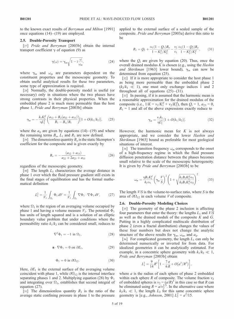
[42] In Figure 1, we give an example of Qp�1 and vp as

determined using the double-porosity theory. The examplemodels a consolidated sandstone phase 1 host that containsthin lenses (squashed/oblate spheroids) of an uncementedgranular phase 2 material. The drained properties of phase 2are determined using the modified Walton theory given inAppendix A. In this way, the moduli K2

d and G2 arefunctions of the background effective stress level Pe. Thehost phase 1 is modeled using f1 = 0.20 and c = 2 in themodel given in Appendix A. All mineral moduli are taken tobe that of quartz Ks = 38 GPa and Gs = 44 GPa and thepermeability of the host phase is k1 = 10 mdarcy. Thedrained properties of the composite were modeled usingthe Hashin and Shtrikman [1963] lower bounds given inequations (21) and (22). The penny-shaped inclusion ofphase 2 have the following geometric properties: a = 3 cm,e = 10�2, v2 = 3%, L1 = 8.6 mm, and V/S = 5 mm. Thespecific shape of the attenuation curve is highly sensitive towhether L1 is greater than or less than V/S. The invariantpeak near 106 Hz is that due to the Biot loss (fluidequilibration at the scale of the seismic wavelength), whilethe broad principal peak that changes with the effectivepressure Pe is that due to mesoscopic-scale equilibration.All dependence on Pe in this example comes from how K2

d

and G2 vary with Pe.[43] The level of attenuation in the double-porosity theory

is controlled by the factors that allow phase 2 to develop adifferent fluid pressure response as compared to phase 1. InFigure 2, this is demonstrated by comparing phase 2modeled as spheres to phase 2 modeled as penny-shapedlenses. Both examples have identically the same volumefractions of phase 2 as well as phase 1 and 2 materialproperties. The difference is that in the sphere model, theHashin and Shtrikman [1963] upper bound is used for Kand G while the lower bound is used in the penny-shapedlens model. A compliant sphere of phase 2 is protected froman applied compression by the rigidity of the phase 1 hostthat surrounds it. Accordingly, not much fluid pressuredifference is created between the two phases and so thereis only a small amount of mesoscopic loss.[44] In modeling the penny-shaped inclusions in Figure 2,

we have used the parameter values a = 3 cm (inclusionradius) and e = 10�1 to obtain V/S = 5 cm and L1 = 0.9 cm.In this case, V/S > L1 which has changed considerably thelook of the attenuation curve as compared to Figure 1 where


6 of 19

B01201

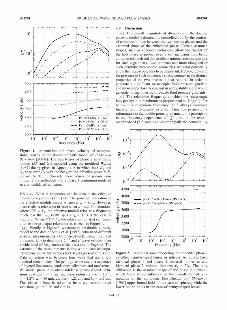
V/S < L1. What is happening can be seen in the effectivemoduli of equations (11)–(13). The principal relaxation inthe effective moduli occurs whenever w = g/aij. However,there is also a relaxation in g(w) when w = wm. For situationswhere V/S � L1, the effective moduli relax at a frequencymuch less than wm (with g(w) = gm). This is the case inFigure 2. When V/S < L1, the relaxation in g(w) can beginprior to the principal relaxation as is seen in Figure 1.[45] Finally, in Figure 3, we compare the double-porosity

model to the data of Sams et al. [1997], who used differentseismic measurements (VSP, cross-well, sonic log, andultrasonic lab) to determine Q�1 and P wave velocity overa wide band of frequencies at their test site in England. Thevariance of the measurements falling within each rectangu-lar box are due to the various rock layers present at this site.Data collection was between four wells that are a fewhundred meters deep. The geology at the site is a sequenceof layered limestones, sandstones, siltstones and mudstones.We model phase 2 as unconsolidated penny-shaped inclu-sions in which a = 5 cm (inclusion radius), e = 6 � 10�3,v2 = 1.2%, k1 = 80 mdarcy, V/S = 1.25 cm, and L1 = 1.45 cm.The phase 1 host is taken to be a well-consolidatedsandstone (f1 = 0.20 and c = 1).

2.9. Discussion

[46] The overall magnitude of attenuation in the double-porosity model is dominantly controlled both by the contrastof compressibilities between the two porous phases and theassumed shape of the embedded phase. Certain assumedshapes, such as spherical inclusions, allow the rigidity ofthe host phase to protect even a soft inclusion from beingcompressedmuch and this results inminimalmesoscopic lossfor such a geometry. Less compact and more elongated oreven dendritic mesoscopic geometries are what potentiallyallow the mesoscopic loss to be important. However, even inthe presence of such structure, a strong contrast in the drainedproperties of the two phases is also required in order togenerate a significant mesoscopic fluid pressure gradientand mesoscopic loss. A contrast in permeability alone wouldgenerate no such mesoscopic-scale fluid pressure gradients.[47] The relaxation frequency at which the mesoscopic

loss per cycle is maximum is proportional to k1/(hL12). Far

below this relaxation frequency, Q�1 always increaseslinearly with frequency as fh/k1. Thus the permeabilityinformation in the double-porosity attenuation is principallyin the frequency dependence of Q�1, not in the overallmagnitude of Q�1, and involves principally the permeability

Figure 1. Attenuation and phase velocity of compres-sional waves in the double-porosity model of Pride andBerryman [2003a]. The thin lenses of phase 2 have framemoduli (K2

d and G2) modeled using the modified Walton[1987] theory given in Appendix A in which both K2

d andG2 vary strongly with the background effective pressure Pe

(or overburden thickness). These lenses of porous con-tinuum 2 are embedded into a phase 1 continuum modeledas a consolidated sandstone.

Figure 2. A comparison of modeling the embedded phase 2as either penny-shaped lenses or spheres. All curves haveidentical phase 1 and phase 2 material properties andidentical phase 2 volume fractions v2 = 2%. The onlydifference is the assumed shape of the phase 2 inclusionwhich has a strong influence on the overall drained bulkmodulus of the composite (the Hashin and Shtrikman[1963] upper bound holds in the case of spheres, while thelower bound holds in the case of penny-shaped lenses).


7 of 19

B01201

k1 of the host phase, not the overall permeability of thecomposite (see Berryman [1988] for a related discussion). Ifphase 2 is well modeled as being small penny-shapedinclusions embedded in phase 1, then k1 is controlling theoverall permeability. If phase 2 corresponds to throughgoingconnected joints, then although Q�1(w) contains informa-tion about k1, it does not contain information about theoverall permeability which is being dominated by k2 in thiscase (i.e., k2 has no significant influence on the mesoscopicloss process).[48] In the case of throughgoing joints, the equilibration

at the scale of the wavelength (the Biot loss) has a chance ofbeing shifted to lower frequencies. The only way to deter-mine the proper attenuation curve in this case is to solve thecubic characteristic equation for s2 (the characteristic equa-tion is obtained by inserting a plane wave solution into thecomplete double-porosity equations (6)–(10), as discussedearlier).

3. Patchy Saturation Model

[49] Another important source of mesoscopic-scale het-erogeneity having an important influence on seismic prop-

erties is patchy fluid saturation [e.g., Knight et al., 1998].All natural hydrological processes by which one fluid non-miscibly invades a region initially occupied by anotherresult in a patchy distribution of the two fluids. The patchsizes are distributed across the entire range of mesoscopiclength scales and for many invasion scenarios are expectedto be fractal. As a compressional wave squeezes such amaterial, the patches occupied by the less compressible fluidwill respond with a greater fluid pressure change than thepatches occupied by the more compressible fluid. The twofluids will then equilibrate by the same type of mesoscopicflow already modeled in the double-porosity model.[50] An analysis almost identical to that of Pride and

Berryman [2003a, 2003b] can be carried out that leads tothe same effective poroelastic moduli given by equations(11)–(13) but with different definitions of the aij constantsand internal transport coefficient g(w). In the model, a singleuniform porous frame is saturated by mesoscopic-scalepatches of fluid 1 and fluid 2. We define porous phase 1 tobe those regions (patches) occupied by the less mobile fluidand phase 2 the patches saturated by the more mobile fluid,i.e., by definition, h1 > h2. This most often (but not necessar-ily) corresponds to Kf1 > Kf2 and therefore to B1 > B2.[51] Johnson [2001] has treated this model using a

different coarse-graining argument while starting from thesame local physics (however, he assumes the porous mate-rial is a Gassmann monomineral material). Our finalundrained bulk modulus is identical to the result of Johnson[2001] in the limits of high and low frequency and differsonly negligibly in the transition range of frequencies wherethe flow in either model is not explicitly treated.

3.1. Patchy Saturation aij Coefficients

[52] To obtain the aij for the patchy saturation model, wenote that by model assumption, each patch has the same aand K. The poroelastic differences between patches isentirely due to B1 being different than B2. Upon averagingequation (3) and using r � v = r � (v1 _�u1) + r � (v2 _�u2),where an overline again denotes a volume average overthe appropriate phase, and using the fact that the aij aredefined in the extreme high-frequency limit where the fluidshave no time to traverse the internal interface @�12 (i.e., theaij are defined under the condition that _zint = 0), one has

r � v ¼ � v1

K_pc1 �

v2

K_pc2 þ

v1aK

_pf 1 þv2aK

_pf 2; ð42Þ

r � q1 ¼v1aK

_pc1 �v1aKB1

_pf 1; ð43Þ

r � q2 ¼v2aK

_pc2 �v2aKB2

_pf 2: ð44Þ

The average confining pressures �pci in each phase are not apriori known; however, they are necessarily linear functionsof the three independent applied pressures of the theoryPc(= v1�pc1 + v2�pc2), �pf1, and �pf2. It is straightforward todemonstrate that if and only if the average confiningpressures take the form

v1 _pc1 ¼ v1 _Pc þ b _pf 1 � b _pf 2 ð45Þ

v2 _pc2 ¼ v2 _Pc � b _pf 1 þ b _pf 2; ð46Þ

Figure 3. Attenuation and dispersion predicted by thedouble-porosity model of Pride and Berryman [2003a](the solid curves) as compared to the data of Sams et al.[1997] (rectangular boxes). The number of Q�1 estimatesdetermined by Sams et al. [1997] falling within eachrectangular box are 40 VSP, 69 cross-well, 854 sonic log,and 46 ultrasonic core measurements. A similar number ofvelocity measurements were made. These various measure-ments come from different depth ranges at their test site.


8 of 19

B01201

will equations (42)–(44) produce aij that satisfy thethermodynamic symmetry requirement of aij = aji (i.e.,these aij constants are all second derivatives of a strainenergy function as demonstrated by Pride and Berryman[2003a]). Upon placing equations (45) and (46) intoequations (42)–(44), we then have

a11 ¼ 1=K; ð47Þ

a22 ¼ �bþ v1=B1ð Þa=K; ð48Þ

a33 ¼ �bþ v2=B2ð Þa=K; ð49Þ

a12 ¼ �v1a=K; ð50Þ

a13 ¼ �v2a=K; ð51Þ

a23 ¼ ba=K; ð52Þ

where b is the single constant remaining to be determined.[53] To obtain b, we note that in the high-frequency limit,

each local patch of phase i is undrained and thus charac-terized by an undrained bulk modulus Ki

u = K/(1 � aBi)and a shear modulus G that is the same for all patches. Inthis limit, the usual laws of elasticity (as opposed to those ofporoelasticity) govern the response of the composite. Notethat, even if the rock frame is spatially uniform, an excep-tion to uniform G can, in principle, occur if cracks areuniformly present. In this case, it is known [see Berryman etal., 2002] that the shear modulus in the regions containingdry cracks can be somewhat different from the shearmodulus in the regions containing wet cracks. In reality,however, all cracks tend to be water wet in partiallysaturated rocks and it is a physically reasonable approxi-mation to assume that G is the same for each phase evenwhen cracks are present.[54] Under these precise conditions (elasticity of an

isotropic composite having uniform G and all heterogeneityconfined to the bulk modulus which in the present casecorresponds to Ki

u), we follow Johnson [2001] by invokingthe theorem of Hill [1963], which states that the overallundrained-unrelaxed modulus of the composite KH is givenexactly by

1

KH þ 4G=3¼ v1

Ku1 þ 4G=3

þ v2

Ku2 þ 4G=3

: ð53Þ

In terms of the aij, this same undrained-unrelaxed Hillmodulus is given by

1

KH

¼ a11 þ a12dpf 1dPc

� �U

þ a13dpf 2dPc

� �U

; ð54Þ

where upon using r � qi = 0 and _zint = 0 in equation (8) andthen using (47)–(52), the undrained-unrelaxed pressureratios are

dpf 1dPc

� �U

¼ b� v1v2=B2

b v1=B1 þ v2=B2ð Þ � v1v2= B1B2ð Þ ð55Þ

dpf 2dPc

� �U

¼ b� v1v2=B1

b v1=B1 þ v2=B2ð Þ � v1v2= B1B2ð Þ : ð56Þ

Thus, after some algebra, equation (54) yields the exactresult

b ¼ v1v2v1

B2

þ v2

B1

� �a� 1� K=KHð Þ= v1B1 þ v2B2ð Þa� 1� K=KHð Þ v1=B1 þ v2=B2ð Þ

� �ð57Þ

with KH given by equation (53). All the aij are nowexpressed in terms of known information.

3.2. Patchy Saturation Transport

[55] Next, we must address the internal fluid pressureequilibration between the two phases with the goal ofobtaining the internal transfer coefficient g of equation (9).The mathematical definition of the rate of internal fluidtransfer is

_zint ¼1

V

Z@�12

n �Q1 dS; ð58Þ

where V is the volume occupied by the composite. Apossible concern in the patchy saturation analysis is whethercapillary effects at the local interface @�12 separating thetwo phases need to be considered.3.2.1. Capillary Effects[56] At the pore scale, the interface separating one fluid

patch from the next is a series of meniscii. Roughness on thegrain surfaces keeps the contact lines of these menisciipinned to the grain surfaces. Pride and Flekkoy [1999]argue that the contact lines of an air-water meniscus willremain pinned for fluid pressure changes less than roughly104 Pa, which corresponds to the pressure range induced bylinear seismic waves. So as a wave passes, the meniscii willbulge and change shape but will not migrate away.[57] For the fluid pressure equilibration problem, one

porous continuum boundary condition is that all fluidvolume that locally enters the interface @�12 from one side,must exit the other side so that n � Q1 = n � Q2(= n � Q).Another boundary condition is that the rate at which thefluid pressure difference across the interface is changing isequal to the surface tension multiplied by the rate at whichthe mean curvature of the meniscii is changing. At the levelof the porous continuum, this boundary condition may bewritten [cf. Nagy and Blaho, 1994; Nagy and Nayfeh, 1995;Tserkovnyak and Johnson, 2003]

@pf 1@t

� @pf 2@t

¼ Wn �Q on @�12 ð59Þ

where W is called the membrane stiffness. For cylindricaltube models of the pore space, one has [e.g., Nagy andBlaho, 1994] W = s/k (where s is the surface tension and kis the permeability) showing that surface tension effectsbecome more important in tighter rocks. As W ! 0, thesurface tension provides no resistance to the equilibrationwhile as W ! 1, the interface becomes effectively sealedto flow at all frequencies.[58] Tserkovnyak and Johnson [2003] have performed a

complete analysis of the undrained response problem in thepresence of finite W culminating in an analytic expressionfor the complex frequency-dependent undrained bulkmodulus. The dominant effect of finite W is to increasethe low-frequency undrained modulus while leaving the


9 of 19

B01201

high-frequency limit unchanged since this limit alreadycorresponds to no fluid equilibration. As W ! 1, there isno dispersion in the bulk modulus since the fluid in eachpatch remains in the patch at all frequencies.[59] Here, we only seek to define the precise conditions

for which the surface tension (or capillary) effects may beneglected in the static limit where such effects are the mostimportant. To do so, we follow Tserkovnyak and Johnson[2003] and integrate equation (59) over @�12 and over time.Equation (58) may be employed along with the fact thatpfi(r) = �pfi are spatial constants to give

pf 1 � pf 2 ¼V

SWzint; ð60Þ

where S is the amount of fluid interface within a sample ofvolume V. If this expression for zint is used in equation (8)along with sealed sample conditions (r � q1 =r � q2 = 0), onecan solve for both �pf1 and �pf2 and take their difference. The aijconstants of section 3.1 are unaffected by W since they aredefined in the high-frequency limit of no fluid equilibration.In thismanner, one obtains that the key dimensionless numberC controlling whether �pf1 6¼ �pf2 at low frequencies andtherefore controlling the importance of capillary effects in theelastic response is (assuming B1 > B2)

C ¼ WV

S

a b� v1v2=B2ð ÞK

: ð61Þ

When C � 1, surface tension plays absolutely no role in theeffective moduli.When C� 1, there is no acoustic dispersionor attenuation because the surface tension keeps the fluidpatches from equilibrating. If B2 > B1, one should replace B2

with B1 in the definition of C.[60] One way to be in the limit where surface tension is

negligible is to have the fluid bulk moduli in each patch verysimilar. In this case, b! v1v2/B2 and C! 0. However, in thiscase there is notmuch attenuation and dispersion since there isnot much mesoscopic flow induced by the wave.[61] Using W = s/k for making estimates, one finds that

for surface tension to be negligible the inequality

sV=SkK

< 1 ð62Þ

must hold. Using the common sandstone values of k =100 mdarcy, K = 10 GPa, and s � 10�2 Pa m (order ofmagnitude appropriate for water/air and water/oil meniscii),one obtains that V/S should be smaller than roughly 10�1 mfor surface tension effects to be negligible. In what follows,we only treat the regime C � 1 which is the regime alsostudied by Johnson [2001].3.2.2. Mesoscopic Flow Equations[62] To obtain the transport law�iwzint = g(w) (�pf 1� �pf 2),

the mesoscopic flow is analyzed in the limits of low and highfrequencies. These limits are then connected using a fre-quency function that respects causality constraints. Thelinear fluid response inside the patchy composite due to aseismic wave can always be resolved into two portions:(1) a vectorial response due to macroscopic fluid pressuregradients across an averaging volume that generate a mac-roscopic Darcy flux qi across each phase and that corre-

sponds to the macroscopic conditions �pfi = 0 and r�pfi 6¼ 0;and (2) a scalar response associated with internal fluidtransfer and that corresponds to the macroscopic conditions�pfi 6¼ 0 and r�pfi = 0. The macroscopic isotropy of thecomposite guarantees that there is no cross coupling betweenthe vectorial transport qi and the scalar transport _zint withineach sample (‘‘Curie’s principle’’ which is, in fact, a theorem[cf. deGroot and Mazur, 1984]).[63] The mesoscopic flow problem that defines _zint is the

internal equilibration of fluid pressure between the patcheswhen a confining pressure �P has been applied to a sealedsample of the composite. Having the external surface sealedis equivalent to the required macroscopic constraint thatr�pfi = 0. Upon taking the divergence of equation (2) andusing equation (3), the diffusion problem controlling themesoscopic flow becomes

k

hir2pfi þ iw

aKBi

pfi ¼ iwaKpci in �i; ð63Þ

pfi� �

¼ 0 n � rpfi� �

¼ 0 on @�12; ð64Þ

n � rpfi ¼ 0 on @Ei; ð65Þ

where �i is the region that each phase occupies within theaveraging volume, @Ei is that portion of the external surfaceof the averaging volume that is in contact with phase i, andthe brackets in equation (64) again denote jumps across theinterface. One also needs to insert equations (3) and (4) intoequation (1) to obtain a second-order partial differentialequation for the displacements ui. In general, the localconfining pressures pci are determined using

pci ¼ �Kr � ui þ apfi ð66Þ

once the displacements ui are known.3.2.3. Low-Frequency Limit of ;(W)[64] As w ! 0, we can represent the local fields as

perturbation expansions in the small parameter �iw [e.g.,Johnson, 2001]

pfi ¼ p0ð Þfi � iwp 1ð Þ

fi þ O w2 �

ð67Þ

pci ¼ p0ð Þci � iwp 1ð Þ

ci þ O w2 �

; ð68Þ

and equivalently for ui. The zeroth-order response corre-sponds to uniform fluid pressure in the pores and is thereforegiven by pc1

(0) = pc2(0) = �P and

p0ð Þfi

�P¼ Bo ¼ � a12 þ a13

a22 þ 2a23 þ a33¼ 1

v1=B1 þ v2=B2

; ð69Þ

where the patchy saturation aij have been employed. Thefact that the quasi-static Skempton’s coefficient in thepatchy saturation model is exactly the harmonic averageof the constituents Bi is equivalent to saying that atlow frequencies, the fluid bulk modulus is given by 1/Kf =v1/Kf 1 + v2/Kf 2. The quasi-static response is thus completely


10 of 19

B01201

independent of the spatial geometry of the fluid patches; itdepends only on the volume fractions occupied by thepatches.[65] The leading order correction to uniform fluid pres-

sure is then controlled by the boundary value problem

Kk

ah1r2p

1ð Þf 2 ¼ h2

h11� Bo

B2

� ��P in �2; ð70Þ

Kk

ah1r2p

1ð Þf 1 ¼ 1� Bo

B1

� ��P in �1; ð71Þ

p1ð Þf 1 ¼ p

1ð Þf 2 on @�12; ð72Þ

n � rp1ð Þf 2 ¼ h2

h1n � rp

1ð Þf 1 on @�12; ð73Þ

n � rp1ð Þfi ¼ 0 on @Ei: ð74Þ

It is now assumed that for patchy saturation cases of interest(air/water or water/oil), the ratio h2/h1 can be consideredsmall. To leading order in h2/h1, equations (70), (73), and(74) require that pf 2

(1)(r) = �pf 2(1) (a spatial constant). The

fluid pressure in phase 1 is now rewritten as

p1ð Þf 1 rð Þ ¼ p

1ð Þf 2 � h1a

kK1� Bo

B1

� ��P�1 rð Þ; ð75Þ

where, from equations (71), (72) and (74) and to leadingorder in h2/h1, the potential �1 is the solution of the sameelliptic boundary value problem (28)–(30) given earlier.[66] Upon averaging (75) over all of �1, the leading order

in�iw difference in the average fluid pressures can be written

pf 1 � pf 2

�P¼ �iw

p1ð Þf 1 � p

1ð Þf 2

�P

!¼ iw

h1akK

1� Bo

B1

� �L21; ð76Þ

where L1 is again the length defined by equation (27).[67] To connect this fluid pressure difference to the

increment _zint, we use the divergence theorem and the no-flow boundary condition on @Ei to write equation (58) as

�iwzint ¼iwV

k

h

Z@�12

n � rp1ð Þf 1 dS ¼ iwv1

aK

1� Bo

B1

� ��P: ð77Þ

Replacing �P with �pf 1 � �pf 2 using equation (76) then givesthe desired law �iwzint = gp (�pf 1 � �pf 2) with

gp ¼v1k

h1L211þ O

h2h1

� �� ð78Þ

being the low-frequency limit of interest.3.2.4. High-Frequency Limit of ;(W)[68] It has already been commented that in the extreme

high-frequency limit where each patch behaves as if it weresealed to flow ( _zint = 0), the theory of Hill [1963] applies (solong as all cracks are water wet). Hill demonstrated, amongother things, that when each isotropic patch has the sameshear modulus, the volumetric deformation within eachpatch is a spatial constant. The fluid pressure response inthis limit pfi

1 is thus a uniform spatial constant throughout

each phase except in a vanishingly small neighborhood ofthe interface @�12 where equilibration is attempting to takeplace. The small amount of fluid pressure penetration that isoccurring across @�12 can be locally modeled as a one-dimensional process normal to the interface.[69] Using the coordinate x to measure linear distance

normal to the interface (and into phase 1), one has thatequation (63) is satisfied by [Johnson, 2001]

pf 1 ¼ p1f 1 þ C1eiffiffiffiffiffiffiffiffiffiiw=D1

px ð79Þ

pf 2 ¼ p1f 2 þ C2e�iffiffiffiffiffiffiffiffiffiiw=D1

px; ð80Þ

where the diffusivities are defined Di = kKBi/(hia). Theconstants Ci are found from the continuity conditions (64)to be

C1 ¼�1

1þffiffiffiffiffiffiffiffiffiffiffiffiffiffiffiffiffiffiffiffiffiffiffiffiffih2B2= h1B1ð Þ

p p1f 1 � p1f 2

� �ð81Þ

C2 ¼ffiffiffiffiffiffiffiffiffiffiffiffiffiffiffiffiffiffiffiffiffiffiffiffiffih2B2= h1B1ð Þ

p1þ

ffiffiffiffiffiffiffiffiffiffiffiffiffiffiffiffiffiffiffiffiffiffiffiffiffih2B2= h1B1ð Þ

p p1f 1 � p1f 2

� �: ð82Þ

Although not actually needed here, we have that pfi1 = Bipci,

where the uniform confining pressure of each patch is givenby equations (45) and (46), so that the fluid pressuredifference between the phases goes as

p1f 1 � p1f 2

�P¼ B1 � B2

1� b B1=v1 þ B2=v2ð Þ : ð83Þ

Equation (83) is exactly the difference between equations(55) and (56). Because the penetration distance

ffiffiffiffiffiffiffiffiffiffiDi=w

pvanishes at high frequencies, we may state that to leadingorder in the high-frequency limit, �pf1 � �pf2 = pf1

1 � pf21.

[70] To obtain the high-frequency limit of the transportcoefficient g(w), we use the definition (58) of the internaltransport (note that �n � rpf 1 = @pf 1/@x)

�iwzint ¼1

V

k

h1

Z@�12

@pf 1@x

dS ð84Þ

along with equations (79) and (81). The result is

g wð Þ � i3=2ffiffiffiw

p S

V

ffiffiffiffiffiffiffiffiffiffiffiffiffiffiffiffiffiffiffiffiffiffiffiffiffika= h1B1Kð Þ

p1þ

ffiffiffiffiffiffiffiffiffiffiffiffiffiffiffiffiffiffiffiffiffiffiffiffiffih2B2= h1B1ð Þ

p !

ð85Þ

as w ! 1. Here, S is again the area of @�12 containedwithin a volume V of the patchy composite.3.2.5. Full Model for g(w)[71] The high- and low-frequency limits of g are then

connected by a simple frequency function to obtain the finalmodel

g wð Þ ¼ gp

ffiffiffiffiffiffiffiffiffiffiffiffiffiffiffiffiffiffiffiffi1� iw=wp

q; ð86Þ

where the transition frequency wp is defined

wp ¼B1K

h1ak v1V=Sð Þ2

L411þ

ffiffiffiffiffiffiffiffiffiffih2B2

h1B1

s !2

; ð87Þ

and where gp = v1k/(h1L12). Equation (86) has a single

singularity (a branch point) at w = �iwp. Causality requiresthat with an e�iwt time dependence, all singularities and


11 of 19

B01201

zeroes of a transport coefficient like g(w) must reside in thelower half complex w plane. Equation (86) satisfies thisphysically important constraint.

3.3. Patchy Saturation Modeling Choices

[72] To use the patchy saturation model, appropriatevalues for the two geometric terms L1 and V/S must bespecified. Immiscible fluid distributions in the earth havevery complicated geometries since they arise from slowflow that often produces fractal patch distributions. Inparticular, analytical solutions of the boundary value prob-lem (28)–(30) that defines L1 for such real Earth situationsare impossible. Recall that L1 is a characteristic length ofphase 1 (the phase having the smaller fluid mobility k/h)that defines the distance over which the fluid pressuregradient is defined during the final stages of equilibration.For complicated geometries it may either be numericallydetermined, treated as a target parameter for a full waveforminversion of seismic data, or simply estimated qualitatively.In the numerical examples that follow, we will assume (forconvenience) that the individual patches correspond todisconnected spheres for which simple analytical resultsare available for L1 and V/S.[73] If we consider phase 2 (porous continuum saturated

by the less viscous fluid) to be in the form of spheresof radius a embedded within each radius R sphere of thetwo-phase composite, then v2 = (a/R)3, V/S = av2/3, andL12 = 9v2

�2/3a2/14[1 � 7v21/3/6]. This model is particularly

appropriate when v2 � v1. Since the fluid 2 patches aredisconnected, the definitions (11)–(13) of the effectiveporoelastic moduli again hold. Furthermore, fluid 2 maybe taken to be immobile relative to the framework of grainsin the wavelength-scale Biot equilibration so that the inertialproperties of equations (34) and (35) are identified as rf =rf1, r = (1 � f)rs + f(v1rf1 + v2rf2) and ~r = �h1/(iwk).[74] In situations where it is more appropriate to treat

fluid 1 (the more viscous fluid) as occupying disconnectedpatches (e.g., when v1 � v2), the effective poroelasticmoduli are defined by interchanging 2 and 3 in the sub-scripts of equations (11)–(13). Again assuming the phase 1patches to be spheres of radius a embedded within eachradius R sphere of the two-phase composite, we have thatv1 = (a/R)3 and V/S = av1/3. The elliptic boundary valueproblem (28)–(30) can be solved in this case to give L1

2 =a2/15. Furthermore, the effective inertial coefficients in theBiot theory are defined rf = rf 2, r = (1 � f) rs + f(v1rf1 +v2rf 2), and ~r = �h2/(iwk).[75] In situations where both phases form continuous

paths across each averaging volume, it is best to determinethe attenuation and phase velocity by seeking the planelongtitudinal wave solution of nonreduced ‘‘double-poros-ity’’ governing equations of the form (6)–(10). However,this approach is not pursued here. We conclude by notingthat, if the embedded fluid is fractally distributed, thelengths L1 will remain finite while (V/S)/L1 ! 0 as thefractal surface area S becomes large (however, V/S neverreaches zero because the fractality has a small-scale cutofffixed by the grain size of the material).


[76] In Figure 4 we compare the Johnson [2001] predictionof KU to our own for a consolidated sandstone (frame

properties as determined in Appendix Awith k = 100 mdarcy,c = 10, f = 0.20) in which phase 1 is saturated with water andphase 2 is taken to be spherical regions saturated with air. Thetwo estimates have identical asymptotic dependence in boththe limits of high and low frequencies. In the crossover range,the physics is not precisely modeled in either approach.However, even in the crossover range, the differences in thetwo models is slight.[77] Figure 5 gives the P wave velocity and attenuation

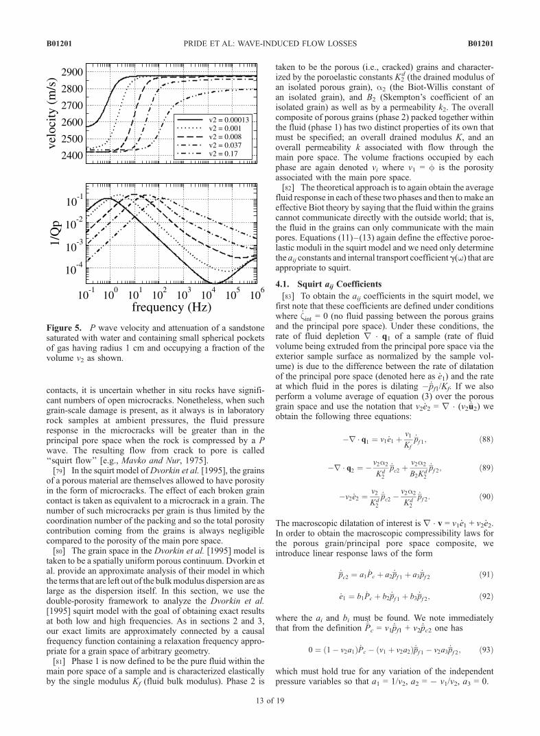
for a model in which the frame properties correspond to k =10 mdarcy, c = 15, and f = 0.15. Phase 2 is saturated by airand is taken to be isolated spheres of radius a = 1 cm.Phase 1 is saturated with water. The volume fraction v2occupied by these 1 cm spheres of gas is as shown in Figure5. Even tiny amounts of gas saturation yield rather largeamounts of attenuation and dispersion; yet these predictionsare consistent with the magnitudes of observed attenuationand dispersion in rocks.

4. Squirt Flow Model

[78] Laboratory samples of consolidated rock often havebroken grain contacts and/or microcracks in the grains.Much of this damage occurs as the rock is brought fromdepth to the surface. Since diagenetic processes in asedimentary basin tend to cement microcracks and grain

Figure 4. Undrained bulk modulus KU (w) in both thepatchy saturation model presented in this article and themodel of Johnson [2001]: (top) Re{KU} and (bottom)QK

�1 = �Im{KU}/Re{KU}. The physical model is 10 cmspherical air pockets embedded within a water-saturatedregion. The volume fraction of gas saturated rock is 3% inthis example. The properties of the rock correspond to a100 mdarcy consolidated sandstone.


12 of 19

B01201

contacts, it is uncertain whether in situ rocks have signifi-cant numbers of open microcracks. Nonetheless, when suchgrain-scale damage is present, as it always is in laboratoryrock samples at ambient pressures, the fluid pressureresponse in the microcracks will be greater than in theprincipal pore space when the rock is compressed by a Pwave. The resulting flow from crack to pore is called‘‘squirt flow’’ [e.g., Mavko and Nur, 1975].[79] In the squirt model ofDvorkin et al. [1995], the grains

of a porous material are themselves allowed to have porosityin the form of microcracks. The effect of each broken graincontact is taken as equivalent to a microcrack in a grain. Thenumber of such microcracks per grain is thus limited by thecoordination number of the packing and so the total porositycontribution coming from the grains is always negligiblecompared to the porosity of the main pore space.[80] The grain space in the Dvorkin et al. [1995] model is

taken to be a spatially uniform porous continuum. Dvorkin etal. provide an approximate analysis of their model in whichthe terms that are left out of the bulkmodulus dispersion are aslarge as the dispersion itself. In this section, we use thedouble-porosity framework to analyze the Dvorkin et al.[1995] squirt model with the goal of obtaining exact resultsat both low and high frequencies. As in sections 2 and 3,our exact limits are approximately connected by a causalfrequency function containing a relaxation frequency appro-priate for a grain space of arbitrary geometry.[81] Phase 1 is now defined to be the pure fluid within the

main pore space of a sample and is characterized elasticallyby the single modulus Kf (fluid bulk modulus). Phase 2 is

taken to be the porous (i.e., cracked) grains and character-ized by the poroelastic constants K2

d (the drained modulus ofan isolated porous grain), a2 (the Biot-Willis constant ofan isolated grain), and B2 (Skempton’s coefficient of anisolated grain) as well as by a permeability k2. The overallcomposite of porous grains (phase 2) packed together withinthe fluid (phase 1) has two distinct properties of its own thatmust be specified; an overall drained modulus K, and anoverall permeability k associated with flow through themain pore space. The volume fractions occupied by eachphase are again denoted vi where v1 = f is the porosityassociated with the main pore space.[82] The theoretical approach is to again obtain the average

fluid response in each of these two phases and then tomake aneffective Biot theory by saying that the fluid within the grainscannot communicate directly with the outside world; that is,the fluid in the grains can only communicate with the mainpores. Equations (11)–(13) again define the effective poroe-lastic moduli in the squirt model and we need only determinethe aij constants and internal transport coefficientg(w) that areappropriate to squirt.

4.1. Squirt aij Coefficients

[83] To obtain the aij coefficients in the squirt model, wefirst note that these coefficients are defined under conditionswhere _zint = 0 (no fluid passing between the porous grainsand the principal pore space). Under these conditions, therate of fluid depletion r � q1 of a sample (rate of fluidvolume being extruded from the principal pore space via theexterior sample surface as normalized by the sample vol-ume) is due to the difference between the rate of dilatationof the principal pore space (denoted here as _e1) and the rateat which fluid in the pores is dilating � _�pf1/Kf. If we alsoperform a volume average of equation (3) over the porousgrain space and use the notation that v2 _e2 = r � (v2 _�u2) weobtain the following three equations:

�r � q1 ¼ v1 _e1 þv1

Kf

_pf 1; ð88Þ

�r � q2 ¼ � v2a2

Kd2

_pc2 þv2a2

B2Kd2

_pf 2; ð89Þ

�v2 _e2 ¼v2

Kd2

_pc2 �v2a2

Kd2

_pf 2: ð90Þ

The macroscopic dilatation of interest is r � v = v1 _e1 + v2 _e2.In order to obtain the macroscopic compressibility laws forthe porous grain/principal pore space composite, weintroduce linear response laws of the form

_pc2 ¼ a1 _Pc þ a2 _pf 1 þ a3 _pf 2 ð91Þ

_e1 ¼ b1 _Pc þ b2 _pf 1 þ b3 _pf 2; ð92Þ

where the ai and bi must be found. We note immediatelythat from the definition _�Pc = v1 _�pf1 + v2 _�pc2 one has

0 ¼ 1� v2a1ð Þ _Pc � v1 þ v2a2ð Þ _pf 1 � v2a3 _pf 2; ð93Þ

which must hold true for any variation of the independentpressure variables so that a1 = 1/v2, a2 = � v1/v2, a3 = 0.

Figure 5. P wave velocity and attenuation of a sandstonesaturated with water and containing small spherical pocketsof gas having radius 1 cm and occupying a fraction of thevolume v2 as shown.


13 of 19

B01201

[84] To obtain the bi, we now combine the above into themacroscopic laws

�r � v ¼ �v1b1 þ1

Kd2

� �_Pc � v1b2 þ

v1

Kd2

� �_pf 1 � v1b3 þ

v2a2

Kd2

� �_pf 2;

ð94Þ

�r � q1 ¼ v1b1 _Pc þ v1b2 þv1

Kf

� �_pf 1 þ v1b3 _pf 2; ð95Þ

�r � q2 ¼�a2

Kd2

_Pc þv1a2

Kd2

_pf 1 þv2a2

Kd2B2

_pf 2 ð96Þ

and use the fact that the coefficients of the matrix must besymmetric (aij = aji). With a11 = 1/K corresponding to theoverall drained frame modulus of the composite (to beindependently specified), we obtain v1b1 = �(1/K � 1/K2

d),v1b2 = 1/K � (1 + v1)/K2

d, and b3 = a2/K2d. The final aij

coefficients are exactly

a11 ¼ 1=K; ð97Þ

a22 ¼ 1=K � 1þ v1ð Þ=Kd2 þ v1=Kf ; ð98Þ

a33 ¼v2a2

B2Kd2

; ð99Þ

a12 ¼ �1=K þ 1=Kd2 ; ð100Þ

a13 ¼ �a2=Kd2 ; ð101Þ

a23 ¼ v1a2=Kd2 : ð102Þ

Reasonable models for K and K2d will be discussed shortly.

4.2. Squirt Transport

[85] We next must obtain the coefficient g(w) in themesoscopic transport law �iw zint = g(w) (�pf1 � �pf2). Again,the approach is to first obtain the limiting behavior at lowand high frequencies and then to connect the two limits by asimple function.[86] The fluid response in phase 1 (the principal pore

space) is governed by the Navier-Stokes equation �rpf1 +hr2v1 = �iwrfv1 and the compressibility law Kfr � v1 =iwpf1 where v1 is the local fluid velocity in the pores. Sincefor all frequencies of interest we have that w � Kf /h (notethat Kf /h � 1012 s�1 for liquids and 1010 s�1 for gases), thefluid pressure in phase 1 is governed by the wave equation

r2pf 1 þ w2rfKf

pf 1 ¼ 0; ð103Þ

and since the acoustic wavelength in the fluid is alwaysmuch greater than the grain sizes, the fluid pressure in theprincipal pore space satisfies pf1(r) = �pf1 (a spatial constant)at all frequencies.[87] The focus, then, is on determining the flow and fluid

pressure within the cracked grains (phase 2) that is governedby the local porous continuum laws Q2 = �(k2/h)rpf2 and

k2

hr2pf 2 þ iw

a2

Kd2B2

pf 2 ¼ �iwa2

Kd2

pc2; ð104Þ

where pc2 = �K2dr � u2 + a2pf2. This deformation and

pressure change is excited by applying a uniform normal

stress ��Pn to the surface of the averaging volume withthe fluid pressure satisfying the boundary conditions n �rpf2(r) = 0 on @E2 and pf2(r) = �pf1 on @�12.4.2.1. Low-Frequency Limit of ;(W)[88] The fluid pressure and confining pressure in the

grains can again be developed as a power series in �iw(as in equations (67)–(68)). The zero-order response corre-sponds to the static limit in which the fluid pressure iseverywhere the same and given by pf2

(0) = �pf1 = Bo�P withBo = �(a12 + a13)/(a22 + 2a23 + a33) and with the aij asgiven by equations (97)–(102). The detailed result for Bo

can be expressed

1=K � 1� a2ð Þ=Kd2

Bo

¼ 1

K� 1� a2ð Þ

Kd2

þ v11

Kf

� 1� a2ð ÞKd2

� �

þ v2a2

Kd2

1

B2

� 1

� �; ð105Þ

which reduces to the standard Gassmann expression givenin Appendix A (with a total porosity given by v1 + f2v2),when B2 and a2 are themselves given by the Gassmannexpressions. In this same zero-order limit, the undrainedbulk modulus is defined as 1/Ko

u = a11 + (a12 + a13)Bo,which also reduces to the standard Gassmann expression,when B2 and a2 are themselves given by Gassmannexpressions.[89] The leading order in �iw correction to uniform fluid

pressure is thus governed by the problem

r2p1ð Þf 2 ¼ ha2

k2Kd2

p0ð Þc2 ; ð106Þ

n � rp1ð Þf 2 ¼ 0 on @E2; ð107Þ

p1ð Þf 2 ¼ 0 on @�12: ð108Þ

Here, pc2(0) is the local confining pressure in the grain space

in the static limit that can be written pc2(0)(r) = �pc2

(0) + dP(r).The average static confining pressure throughout thegrains is determined from equation (84) with Pc = �Pand pf 2 = pf1 = Bo�P to yield

p0ð Þc2 ¼ 1� v1Boð Þ

v2�P: ð109Þ

The deviations dP(r) thus integrate by volume to zero dP =0 and are formally defined

dP rð Þ ¼ � 1� v1 þ v2a2ð ÞBo

v2

� ��P � Kd

2

a2

r � u 0ð Þ rð Þ: ð110Þ

The local perturbations dP(r) are thus highly sensitive to thedetailed nature of the grain packing and grain geometry.Fortunately, the details of these perturbations do not play animportant role in the theory.[90] The fluid pressure in the grains is now written in the

scaled form

p1ð Þf 2 rð Þ ¼ � ha2 1� v1Boð Þ

v2k2Kds

�P� rð Þ; ð111Þ


14 of 19

B01201

where the potential �(r) is independent of �P and is asolution of the elliptic problem

r2� rð Þ ¼ �1� v2

1� v1Bo

dP rð Þ�P

; ð112Þ

n � r� ¼ 0 on @E2; ð113Þ

� ¼ 0 on @�12: ð114Þ

To leading order in �iw, an average of equation (111) gives

pf 1 � pf 2 ¼ iwp 1ð Þf 2 þ O w2

�¼ �iw

ha2 1� v1Boð Þv2k2Kd

s

L22�P þ O w2 �

; ð115Þ

where the squared length L22 is defined

L22 ¼ � ¼ �o 1þ v2

1� v1Bo

�odP�o�P

� �; ð116Þ

with overlines denoting volume averages over the grainspace and with the potential �o defined as the solution of

r2�o ¼ �1; ð117Þ

n � r�o ¼ 0 on @E2; ð118Þ

�o ¼ 0 on @�12: ð119Þ

Although it is not generally true that �odP = 0 for all graingeometries, we nevertheless expect this integral to be smallin general because �o is a smooth function and dP = 0. Thelocal perturbations in the static confining pressure dP(r)require a solution of the static displacements throughout theentire grain space, a daunting numerical task. Wheneverthe length L2 needs to be estimated, such as in the numericalresults that follow, our approach is simply to use thereasonable approximation that L2

2 = ��o.[91] Last, from the definition _zint of the internal transfer

we have that to leading order in �iw:

�iwzint ¼iwk2Vh

Z@�12

n � rp1ð Þf 2 dS

¼ �iwk2Vh

Z�2

r2p1ð Þf 2 dV ¼ �iw

a2

Kd2

v2p0ð Þc2

¼ v2k2

hL22pf 1 � pf 2

� �; ð120Þ

where equation (120) follows from equations (109)and (115). The desired result is thus limw!0 g(w) = gsq =v2k2/(hL2

2).4.2.2. High-Frequency Limit of ;(W)[92] In the extreme high-frequency limit, the fluid has no

time to escape in significant amounts from the porous grains(phase 2) and enter the main pore space (phase 1). As such,the fluid pressure distribution in each phase is reasonablymodeled as

pf 1 rð Þ ¼ B11 �P ð121Þ

pf 2 rð Þ ¼ B12 �P þ C2�Pe�i3=2

ffiffiffiffiffiffiffiffiw=D2

px; ð122Þ

where x is again a local coordinate measuring distancenormal to the interface @�12 and where D2 is the fluidpressure diffusivity within the porous grains that is given byD2 = k2K2

dB2/(ha2). In reality, the local confining pressure

pc2(r) throughout the grains has spatial fluctuations aboutthe average value and we have made the approximation thatthe average fluid pressure throughout the grain space isB2pc2(r) � B2

1�P. It is easy to demonstrate that underundrained and unrelaxed conditions,

B11 ¼ a13a23 � a33a12

a22a33 � a223ð123Þ

B12 ¼ a12a23 � a22a13

a22a33 � a223: ð124Þ

However, since these Bi1 do not appear in the final result,

they will not be algebraically developed.[93] The continuity of fluid pressure pf 2 = pf 1 along @�12

(x = 0) requires that C2 = B11 � B2

1. The definition of _zintmay now be used to write

�iwzint ¼1

V

Z@�12

k2

h@p2@x

¼ k2

hi3=2

ffiffiffiffiffiffiwD2

rS

VB11 � B1

2

��P

¼ i3=2ffiffiffiw

pffiffiffiffiffiffiffiffiffiffiffiffiffik2a2

hB2Kd2

sS

Vpf 1 � pf 2

� �; ð125Þ

where we have used, to leading order in the high-frequencylimit, �pf 1 � �pf 2 = (B1

1 � B21)�P. The desired result is then

g wð Þ � S

V

ffiffiffiffiffiffiffiffiffiffiffiffiffiffiffiffiffi�iwk2a2

hB2Kds

sð126Þ

as w ! 1.4.2.3. Full Model for g(w)[94] The high- and low-frequency limits are again caus-

ally connected via the simple function

g wð Þ ¼ gsq

ffiffiffiffiffiffiffiffiffiffiffiffiffiffiffi1� iw

wsq

s; ð127Þ

but now the parameters are defined as

gsq ¼v2k2

hL22ð128Þ

wsq ¼B2K

d2

ha2

k2

L22

v2V=S

L2

� �2

: ð129Þ

4.3. Squirt Flow Modeling Choices

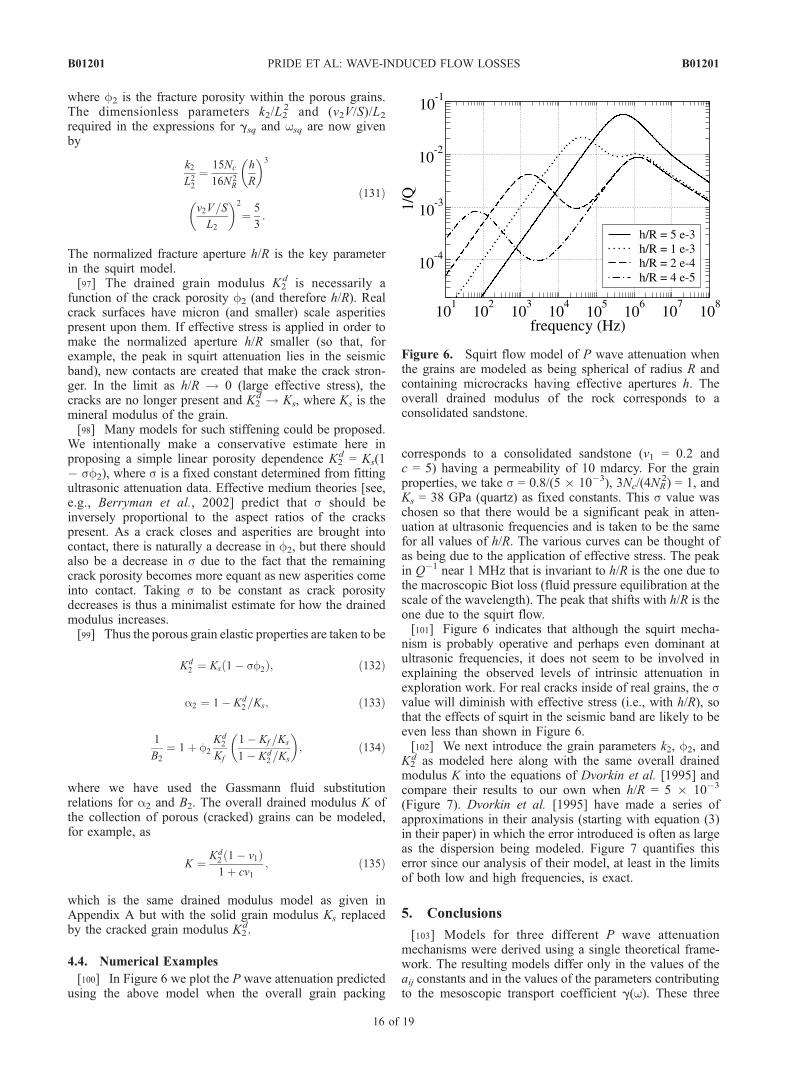
[95] To make numerical predictions of attenuation anddispersion, models must be proposed for the phase 2(porous grain) parameters.[96] If the grains are modeled as spheres of radius R, the

fluid pressure gradient length within the grains can beestimated as L2 = R/

ffiffiffiffiffi15

pand the volume to surface ratio

as V/S = R/(3v2). The grain porosity is assumed to be in theform of microcracks and so it is natural to define aneffective aperture h for these cracks. If the cracks have anaverage effective radius of R/NR (where NR is roughly 2 or 3)and if there are on average Nc cracks per grain (where Nc isalso roughly 2 or 3), then the permeability and porosity ofthe grains are reasonably modeled as

f2 ¼3Nc

4N2R

h

R

k2 ¼ f2h2=12;

ð130Þ


15 of 19

B01201

where f2 is the fracture porosity within the porous grains.The dimensionless parameters k2/L2

2 and (v2V/S)/L2required in the expressions for gsq and wsq are now givenby

k2

L22¼ 15Nc

16N2R

h

R

� �3

v2V=S

L2

� �2

¼ 5

3:

ð131Þ

The normalized fracture aperture h/R is the key parameterin the squirt model.[97] The drained grain modulus K2

d is necessarily afunction of the crack porosity f2 (and therefore h/R). Realcrack surfaces have micron (and smaller) scale asperitiespresent upon them. If effective stress is applied in order tomake the normalized aperture h/R smaller (so that, forexample, the peak in squirt attenuation lies in the seismicband), new contacts are created that make the crack stron-ger. In the limit as h/R ! 0 (large effective stress), thecracks are no longer present and K2

d ! Ks, where Ks is themineral modulus of the grain.[98] Many models for such stiffening could be proposed.

We intentionally make a conservative estimate here inproposing a simple linear porosity dependence K2

d = Ks(1� sf2), where s is a fixed constant determined from fittingultrasonic attenuation data. Effective medium theories [see,e.g., Berryman et al., 2002] predict that s should beinversely proportional to the aspect ratios of the crackspresent. As a crack closes and asperities are brought intocontact, there is naturally a decrease in f2, but there shouldalso be a decrease in s due to the fact that the remainingcrack porosity becomes more equant as new asperities comeinto contact. Taking s to be constant as crack porositydecreases is thus a minimalist estimate for how the drainedmodulus increases.[99] Thus the porous grain elastic properties are taken to be

Kd2 ¼ Ks 1� sf2ð Þ; ð132Þ

a2 ¼ 1� Kd2=Ks; ð133Þ

1

B2

¼ 1þ f2

Kd2

Kf

1� Kf =Ks

1� Kd2=Ks

� �; ð134Þ

where we have used the Gassmann fluid substitutionrelations for a2 and B2. The overall drained modulus K ofthe collection of porous (cracked) grains can be modeled,for example, as

K ¼ Kd2 1� v1ð Þ1þ cv1

; ð135Þ

which is the same drained modulus model as given inAppendix A but with the solid grain modulus Ks replacedby the cracked grain modulus K2

d.


[100] In Figure 6 we plot the P wave attenuation predictedusing the above model when the overall grain packing

corresponds to a consolidated sandstone (v1 = 0.2 andc = 5) having a permeability of 10 mdarcy. For the grainproperties, we take s = 0.8/(5 � 10�3), 3Nc/(4NR

2) = 1, andKs = 38 GPa (quartz) as fixed constants. This s value waschosen so that there would be a significant peak in atten-uation at ultrasonic frequencies and is taken to be the samefor all values of h/R. The various curves can be thought ofas being due to the application of effective stress. The peakin Q�1 near 1 MHz that is invariant to h/R is the one due tothe macroscopic Biot loss (fluid pressure equilibration at thescale of the wavelength). The peak that shifts with h/R is theone due to the squirt flow.[101] Figure 6 indicates that although the squirt mecha-

nism is probably operative and perhaps even dominant atultrasonic frequencies, it does not seem to be involved inexplaining the observed levels of intrinsic attenuation inexploration work. For real cracks inside of real grains, the svalue will diminish with effective stress (i.e., with h/R), sothat the effects of squirt in the seismic band are likely to beeven less than shown in Figure 6.[102] We next introduce the grain parameters k2, f2, and

K2d as modeled here along with the same overall drained

modulus K into the equations of Dvorkin et al. [1995] andcompare their results to our own when h/R = 5 � 10�3

(Figure 7). Dvorkin et al. [1995] have made a series ofapproximations in their analysis (starting with equation (3)in their paper) in which the error introduced is often as largeas the dispersion being modeled. Figure 7 quantifies thiserror since our analysis of their model, at least in the limitsof both low and high frequencies, is exact.

5. Conclusions

[103] Models for three different P wave attenuationmechanisms were derived using a single theoretical frame-work. The resulting models differ only in the values of theaij constants and in the values of the parameters contributingto the mesoscopic transport coefficient g(w). These three

Figure 6. Squirt flow model of P wave attenuation whenthe grains are modeled as being spherical of radius R andcontaining microcracks having effective apertures h. Theoverall drained modulus of the rock corresponds to aconsolidated sandstone.


16 of 19

B01201

models correspond to (1) mesoscopic-scale heterogeneity inthe frame moduli (‘‘double porosity’’), (2) mesoscopic-scaleheterogeneity in the fluid type (‘‘patchy saturation’’), and(3) grain-scale heterogeneity due to microcracks in thegrains (‘‘squirt’’). In all three models, the amount ofattenuation is controlled principally by the contrast of elasticcompressibility among the constituents along with theassumed mesoscopic geometry. In the double-porositymodel, it is necessary that the embedded phase have anelongated or squashed form and that the contrast betweenthe frame bulk modulus of the two porous phases is strongin order for the mesoscopic loss to be significant. In thepatchy saturation model, the contrast in the fluid bulkmodulus must be strong (immiscible patches of differentfluids that have nearly identical bulk moduli would notproduce much attenuation), while in the squirt model, it isthe contrast between the drained modulus of an isolatedcracked grain and that of the entire packing of grains thatcontrols the amount of attenuation.[104] Putting in thin lenses of unconsolidated sand grains

into an otherwise consolidated sandstone can produce atten-uation in the seismic band that is comparable to what is

measured in the field even when the embedded phase repre-sents only a small amount of the total volume (<1% volumefractions). Such a model might correspond to a jointedsandstone. Since mesoscopic-scale heterogeneity is ratherubiquitous throughout the earth’s crust, it seems reasonableto suppose that this mechanism may be responsible for mostof the attenuation observed in seismograms. The squirtmechanism produces a great deal of attenuation at theultrasonic frequencies used in laboratory measurements, buthas trouble explaining attenuation in the seismic band. Thisresult is important for some applications of the theory becausethe rate at which the mesoscopic-scale fluid pressure equili-brates is a strong function of the permeability of the porousmaterial. The rate at which microcracks equilibrate with themain pores in squirt flow is not permeability-dependent.This leaves open the possibility of extracting permeabilityinformation from the frequency dependence of seismicallymeasured Q.

Appendix A: Constituent Properties

[105] In order to use the unified double-porosity frame-work of the present paper, it is convenient to have modelsfor the various porous continuum constituent properties.[106] For unconsolidated sands and soils, the frame mod-

uli (drained bulk modulus Kd and shear modulus G) are wellmodeled using the following variant of the Walton [1987]theory (see Pride [2003] for details)

Kd ¼ 1

6

4 1� foð Þ2n2oPo

p4C2s

" #1=3Pe=Poð Þ1=2

1þ 16Pe= 9Poð Þ½ 4n o1=24

ðA1Þ

G ¼ 3Kd=5; ðA2Þ

where Pe is the effective overburden pressure (e.g., Pe =(1 � f)(rs � rf) gh, where g is gravity and h is overburdenthickness) and Po is the effective pressure at which all grain-to-grain contacts are established. For Pe < Po, thecoordination number n (average number of grain contactsper grain) is increasing as (Pe/Po)

1/2. For Pe > Po, thecoordination number remains constant n = no. Theparameter Po is commonly on the order of 10 MPa. AsPo ! 0, the Walton [1987] result is obtained (all contacts inplace starting from Pe = 0). The porosity of the grain pack isfo and the compliance parameter Cs are defined

Cs ¼1

4p1

Gs

þ 1

Ks þ Gs=3

� �ðA3Þ

where Ks and Gs are the mineral moduli of the grains. Forunimodal grain-size distributions and random grain packs,one typically has 0.32 < fo < 0.36 and 8 < no < 11. Inthe numerical examples we use fo = 0.36, no = 9, and Po =10 MPa.[107] For consolidated sandstones, the frame moduli are

modelled in the present paper as (see Pride [2003] for details)

Kd ¼ Ks

1� f1þ cf

; ðA4Þ

G ¼ Gs

1� f1þ 3cf=2

: ðA5Þ

Figure 7. Dispersion (top) in the real parts of the drainedbulk modulus KD (w), (middle) the undrained bulk modulusKU(w), and (bottom) the Skempton’s coefficient B(w) asdetermined both in the present study and by Dvorkin et al.[1995]. The plots were all generated with h/R = 5 � 10�3.Both theories use identically the same input parameters andare treating identically the same model. The present studymay be considered exact in both the low- and high-frequency limits of the model.


17 of 19

B01201

The consolidation parameter c represents the degree ofconsolidation between the grains and lies in the approximaterange 2 < c < 20 for sandstones. If it is necessary to use a cgreater than say 20 or 30, then it is probably better to use themodified Walton theory.[108] The undrained moduli Ku and B are conveniently

and exactly modeled using the Gassmann [1951] theorywhenever the grains are isotropic and composed of a singlemineral. The results are

B ¼ 1=Kd � 1=Ks

1=Kd � 1=Ks þ f 1=Kf � 1=Ks

� ðA6Þ

Ku ¼ Kd

1� B 1� Kd=Ksð Þ ; ðA7Þ

from which the Biot-Willis constant a may be determined tobe a = 1 � Kd/Ks. These Gassmann results are often calledthe ‘‘fluid substitution’’ relations.[109] The dynamic permeability k(w) as modeled by

Johnson et al. [1987] is

k wð Þko

¼ffiffiffiffiffiffiffiffiffiffiffiffiffiffiffiffiffiffiffiffiffi1� i

4

nJ

wwc

r� i

wwc

� ��1

; ðA8Þ

where the relaxation frequency wc, which controls thefrequency at which viscous boundary layers first develop, isgiven by

wc ¼h

rf Fko: ðA9Þ

Here, F is exactly the electrical formation factor when grainsurface electrical conduction is not important and isconveniently (though crudely) modeled using Archie’s lawF = f�m. The cementation exponent m is related to thedistribution of grain shapes (or pore topology) in the sampleand is generally close to 3/2 in clean sands, close to 2 in shalysands, and close to 1 in rocks having fracture porosity (indeed,a reasonable model is m = 3/2 + 1/c). In the numericalmodeling, the parameter nJ is, for convenience, taken to be 8(cylinder model of the pore space).

[110] Acknowledgments. The work of S.R.P. was supported by theDirector, Office of Science, Office of Basic Energy Sciences, of the U.S.Department of Energy under contract DE-AC03-76SF00098. The work ofJ.G.B. was performed under the auspices of the U.S. Department of Energyunder contract W-7405-ENG-48 and supported specifically by the Geo-sciences Research Program of the DOE Office of Basic Energy Sciences,Division of Chemical Sciences, Geosciences and Biosciences. Work ofJ.G.B. also supported in part by the Stanford Exploration Project, while onsabbatical visiting the Geophysics Department at Stanford University. Allthree authors would like to thank the Associate Editor Jack Dvorkin and thetwo referees for having made useful suggestions that improved the paper.

ReferencesBerryman, J. G. (1988), Seismic wave attenuation in fluid-saturated porousmedia, Pure Appl. Geophys., 128, 423–432.

Berryman, J. G., and G. W. Milton (1991), Exact results for generalizedGassmann’s equations in composite porous media with two constituents,Geophysics, 56, 1950–1960.

Berryman, J. G., and H. F. Wang (1995), The elastic coefficients of double-porosity models for fluid transport in jointed rock, J. Geophys. Res., 100,24,611–24,627.

Berryman, J. G., and H. F. Wang (2000), Elastic wave propagation andattenuation in a double-porosity dual-permability medium, Int. J. RockMech. Min. Sci., 37, 63–78.

Berryman, J. G., S. R. Pride, and H. F. Wang (2002), A differential schemefor elastic properties of rocks with dry or saturated cracks, Geophys. J.Int., 151, 597–611.

Biot, M. A. (1956a), Theory of propagation of elastic waves in a fluid-saturated porous solid. I. Low-frequency range, J. Acoust. Soc. Am., 28,168–178.

Biot, M. A. (1956b), Theory of propagation of elastic waves in a fluid-saturated porous solid. II. Higher frequency range, J. Acoust. Soc. Am.,28, 179–191.

Biot, M. A. (1962), Mechanics of deformation and acoustic propagation inporous media, J. Appl. Phys., 33, 1482–1498.

Biot, M. A., and D. G. Willis (1957), The elastic coefficients of the theoryof consolidation, J. Appl. Mech., 24, 594–601.

Bruggeman, D. A. G. (1935), Berechnung verschiedener physikalischerKonstanten von heterogenen Substanzen, Ann. Phys. Leipzig, 24, 636–679.

Budiansky, B., and R. J. O’Connell (1976), Elastic moduli of a crackedsolid, Int. J. Solids Struct., 12, 81–97.

Cadoret, T., G. Mavko, and B. Zinszner (1998), Fluid distribution effect onsonic attenuation in partially saturated limestones, Geophysics, 63, 154–160.

deGroot, S. R., and P. Mazur (1984), Non-equilibrium Thermodynamics,Dover, Mineola, N. Y.

Dutta, N. C., and H. Ode (1979a), Attenuation and dispersion of compres-sional waves in fluid-filled porous rocks with partial gas saturation(White model)—part I: Biot theory, Geophysics, 44, 1777–1788.

Dutta, N. C., and H. Ode (1979b), Attenuation and dispersion of compres-sional waves in fluid-filled porous rocks with partial gas saturation(White model)—part II: Results, Geophysics, 44, 789–805.

Dutta, N. C., and A. J. Seriff (1979), On White’s model of attenuation inrocks with partial gas saturation, Geophysics, 44, 1806–1812.

Dvorkin, J., G. Mavko, and A. Nur (1995), Squirt flow in fully saturatedrocks, Geophysics, 60, 97–107.

Gassmann, F. (1951), Uber die Elastizitat poroser Medien, Vierteljahrsschr.Naturforsch. Ges. Zuerich, 96, 1–23.

Gelinsky, S., and S. A. Shapiro (1997), Dynamic-equivalent mediumapproach for thinly layered saturated sediments, Geophys. J. Int., 128,F1–F4.

Gurevich, B., and S. L. Lopatnikov (1995), Velocity and attenuation ofelastic waves in finely layered porous rocks, Geophys. J. Int., 121,933–947.

Hashin, Z. (1962), The elastic moduli of heterogeneous materials, J. Appl.Mech., 29, 143–150.

Hashin, Z., and S. Shtrikman (1963), A variational approach to the theory ofthe elastic behavior of multiphase materials, J. Mech. Phys. Solids, 11,127–140.

Hill, R. (1963), Elastic properties of reinforced solids: Some theoreticalprinciples, J. Mech. Phys. Solids, 11, 357–372.

Johnson, D. L. (2001), Theory of frequency dependent acoustics in patchy-saturated porous media, J. Acoust. Soc. Am., 110, 682–694.

Johnson, D. L., J. Koplik, and R. Dashen (1987), Theory of dynamicpermeability and tortuosity in fluid-saturated porous media, J. FluidMech., 176, 379–402.

Knight, R., J. Dvorkin, and A. Nur (1998), Acoustic signatures of partialsaturation, Geophysics, 63, 132–138.

Mavko, G., and A. Nur (1975), Melt squirt in the asthenosphere, J. Geo-phys. Res., 80, 1444–1448.

Mavko, G., and A. Nur (1979), Wave attenuation in partially saturatedrocks, Geophysics, 44, 161–178.

Murphy, W. F., III (1982), Effects of partial water saturation on attenuationin Massilon sandstone and Vycor porous-glass, J. Acoust. Soc. Am., 71,1458–1468.

Murphy, W. F., III (1984), Acoustic measures of partial gas saturation intight sandstones, J. Geophys. Res., 89, 1549–1559.

Nagy, P. B., and G. Blaho (1994), Experimental measurements of surfacestiffness on water-saturated porous solids, J. Acoust. Soc. Am., 95, 828–835.

Nagy, P. B., and A. H. Nayfeh (1995), Generalized formula for the surfacestiffness of fluid-saturated porous media containing parallel pore chan-nels, Appl. Phys. Lett., 67, 1827–1829.

Norris, A. N. (1993), Low-frequency dispersion and attenuation in partiallysaturated rocks, J. Acoust. Soc. Am., 94, 359–370.

O’Connell, R. J., and B. Budiansky (1977), Viscoelastic properties of fluid-saturated cracked solids, J. Geophys. Res., 82, 5719–5735.

Pride, S. R. (2003), Relationships between seismic and hydrological proper-ties, in Hydrogeophysics, edited by Y. Rubin and S. Hubbard, pp. 1–31,Kluwer Acad., New York.

Pride, S. R., and J. G. Berryman (2003a), Linear dynamics of double-porosity and dual-permeability materials. I. Governing equations andacoustic attenuation, Phys. Rev. E, 68, 036603.


18 of 19

B01201

Pride, S. R., and J. G. Berryman (2003b), Linear dynamics of double-porosity and dual-permeability materials. II. Fluid transport equations,Phys. Rev. E, 68, 036604.

Pride, S. R., and E. G. Flekkoy (1999), Two-phase flow through porousmedia in the fixed-contact-line regime, Phys. Rev. E, 60, 4285–4299.

Quan, Y., and J. M. Harris (1997), Seismic attenuation tomography usingthe frequency shift method, Geophysics, 62, 895–905.

Roscoe, R. (1973), Isotropic composites with elastic or viscoelastic phases:General bounds for the moduli and solutions for special geometries,Rheol. Acta, 12, 404–411.

Sams, M. S., J. P. Neep, M. H. Worthington, and M. S. King (1997), Themeasurement of velocity dispersion and frequency-dependent intrinsicattenuation in sedimentary rocks, Geophysics, 62, 1456–1464.

Sato, H., and M. Fehler (1998), Seismic wave propagation and scattering inthe heterogeneous earth, Springer-Verlag, New York.

Skempton, A. W. (1954), The pore-pressure coefficients A and B, Geotech-nique, 4, 143–147.

Thompson, A. H., A. J. Katz, and C. E. Krohn (1987), The microgeometryand transport properties of sedimentary rock, Adv. Phys., 36, 625–694.

Tserkovnyak, Y., and D. L. Johnson (2003), Capillary forces in the acous-tics of patchy-saturated porous media, J. Acoust. Soc. Am., 114, 2596–2606.

Walton, K. (1987), The effective elastic moduli of a random packing ofspheres, J. Mech. Phys. Solids, 35, 213–226.

White, J. E. (1975), Computed seismic speeds and attenuation in rocks withpartial gas saturation, Geophysics, 40, 224–232.

White, J. E., N. G. Mikhaylova, and F. M. Lyakhovitsky (1975), Low-frequency seismic waves in fluid-saturated layered rocks, Izvestija Acad-emy of Sciences USSR, Phys. Solid Earth, 11, 654–659.

Williams, K. L., D. R. Jackson, E. I. Thorsos, D. Tang, and S. G. Schock(2002), Comparison of sound speed and attenuation measured in a sandysediment to predictions based on the Biot theory of porous media, IEEEJ. Ocean. Eng., 27, 413–428.

Wu, R. S., and K. Aki (1988), Multiple scattering and energy transfer ofseismic waves: separation of scattering effect from intrinsic attenuation.II. Application of the theory to Hindu Kush region, Pure Appl. Geophys.,128, 49–80.

��J. G. Berryman, University of California, Lawrence Livermore National

Laboratory, P. O. Box 808 L-200, USA. ([email protected])J. M. Harris, Department of Geophysics, Stanford University, Stanford,

CA 94305, USA. ([email protected])S. R. Pride, Lawrence Berkeley National Laboratory, Earth Sciences

Division, 1 Cyclotron Road MS 90-1116, Berkeley, CA 94720, USA.([email protected])


19 of 19

B01201

seismic attenuation due to wave-induced flowsantos/research/fracture...seismic attenuation due to...

Documents