seismic and petro -physical studies on seismic wave...
TRANSCRIPT

Seismic and PetroSeismic Wave Attenuation
Thesis submitted in accordance with the requirements of
For the award of the D
Wasiu
Seismic and Petro-physical Studies on Seismic Wave Attenuation
Thesis submitted in accordance with the requirements of
ward of the Degree of Doctor of Philosophy
By
Wasiu Olanrewaju RAJI
July 2012
i
physical Studies on Seismic Wave Attenuation
Thesis submitted in accordance with the requirements of
Doctor of Philosophy

ii
TABLE OF CONTENT ii
LIST OF FIGURES v
LIST OF TABLES ix
LIST OF APPENDICES x
DEDICATION xi
ACKNOWLEDGEMENTS xii
ABSTRACT xiv
CHAPTER ONE: INTRODUCTION
1.1: Introduction 2
1.2: Research motivation and aims of the thesis 5
1.3: Thesis structure 6
CHAPTER TWO: SEISMIC ATTENUATION: THEORY, MECHANISM , AND DESCRIPTION 2.1: Phenomenon of attenuation 9
2.1.1: Scattering attenuation 10
2.1.2: Intrinsic attenuation 12
2.2: Describing attenuation with the quality factor, Q 13
2.3: Absorption properties (Q) of the Earth and its effects on the seismic
Waveform 16
2.4: Review of techniques for Q measurement in seismic data 20
2.4.1: Wavelet modelling method 21
2.4.2: Rise time method 22
2.4.3: Analytical signal method 23
2.4.4: Spectral ratio method 24
2.4.5: Frequency shift method 25
2.5: Mechanisms of seismic attenuation 26
2.5.1: Squirt flow mechanism 27
2.5.2: Wave induced fluid flow in random porous media 28
2.5.3: Patchy saturation model 29
2.5.4: Porous – Fracture model 30
2.6: Modulus – Frequency – Dispersion 32

iii
2.6.1: Low frequency elastic modulus 34
2.6.2: High frequency elastic modulus 35
2.6.3: Estimating inverse quality factor (���� from modulus-
frequency- dispersion 38
2.6.4: Irreducible water saturation, ����� 38
CHAPTER THREE: DETERMINATION OF QUALITY FACTOR (Q) IN REFLECTION SEISMIC DATA 3.1: Abstract 43
3.2: Introduction 44
3.3: Theory and methods 48
3.4: Synthetic tests and model comparison 52
3.5: Q measurement in field seismic data 56
3.6: Results and Discussion 63
3.7: Separating scattering attenuation from composite attenuation 65
3.8: Conclusion 68
CHAPTER FOUR: ROCK PHYSICS DIAGNOSTICS, ATTENUATION MEASUREMENT AND ANALYSES IN WELLS
4.1: Abstract 71
4.2: Introduction 71
4.3: Description of some elastic moduli 75
4.4.1: Rock Physics analysis for rock fluid diagnosis 77
4.4.2: Rock physics analyses for pore fluid diagnosis- Discussion of results 86 4.5.1: Attenuation estimation and analysis in wells 87
4.5.2: Attenuation diagnostics and estimation in wells –
Discussion of results 93
4.6: Conclusion 94
CHAPTER FIVE: ENHANCED SEISMIC Q-COMPENSATION
5.1: Abstract 97
5.2: Introduction 98
5.3: The Q-compensation procedure 101

iv
5.4: Q-compensation scheme in a stack of layers 104
5.5: Application to synthetic and field seismic data 107
5.6: Q-compensation and the input layer parameters 114
5.7: Discussion 117
5.8: Conclusion 118
CHAPTER SIX: THE USE OF SEISMIC ATTENUATION FOR MON ITORING SATURATION IN HYDROCARBON RESERVOIRS 6.1: Summary 120
6.2: Introduction 120
6.3: The use of seismogram-derived attenuation for monitoring reservoir
saturation 123
6.4: Effects of other reservoir properties on attenuation 130
6.5: Attenuation calibration: seismic to well logs 133
6.6: Discussion and Conclusion 135
CHAPTER SEVEN: SUMMARY OF RESULTS AND SCOPE FOR FUTURE WORK
7.1: Summary of results 138
7.2: Future work 144
BIBLIOGRAPHY 148
APPENDICES 157

v
LIST OF FIGURES Fig. 2.1: Energy loss in decibel (db) with distance due to attenuation......................................3 Fig. 2.1: Plane wave propagations in elastic and attenuating Earth models. (a) is the trace from elastic model; (b) is the trace from attenuating model. The trace in (b) shows amplitude diminution, delayed arrivals, waveform distortion, and phase reversal compared to the blue plot, due to the effects of attenuation. Q is represented by 30 in all the layers in the attenuating model..................................................................................................................19 Fig. 2.2: Schematic diagram of patchy saturated rock model.................................................34 Fig. 2.3: The estimated compressional modulus versus water saturation using Gassmann (1951) equation. The nearly straight line is the high frequency modulus, while the curved line in is the low frequency modulus..........................................................................................37 Fig. 2.4: The estimated compressional modulus versus water saturation using Vp-substitution equation (Mavko et al., 1995). The nearly straight line is the high frequency modulus, while the curved line in is the low frequency modulus.............................................37 Fig. 2.5: Estimated inverse quality factor Vs. water saturation. The blue plot is from Gassmann (1951) equation, the red plot is from Mavko et al. (1998) equation. Water saturation increases from left to right, while gas saturation increases from right to left of the plot..........................................................................................................................................39 Fig. 2.6: The estimated maximum inverse quality factor versus saturation at 40%, and 80% irreducible water saturation, using Gassmann (1951) equation. The higher the irreducible water saturation, the lower the attenuation..............................................................................41 Fig. 2.7: The estimated maximum inverse quality factor versus saturation at 40%, and 80% irreducible water saturation, using Mavko et al. (1998) equation. The higher the irreducible water saturation, the lower the attenuation...............................................................................41 Fig. 3.1: The frequency spectrum of Ricker wavelet at time 0 (black) and time 2.2s (blue) in an attenuating medium with Q value equals 30....................................................................49 Fig. 3.2: The amplitude spectrum of a Ricker wavelet at time 0 and 2.2s in an attenuating Earth model of Q value equals 30. The signal at 3.2ms is a multiple reflection.....................49 Fig. 3.3: The various spectra shapes used in the attenuation model to represent the real seismic signal. Red is the triangular spectrum, pink is the Ormsby spectrum (or a boxcar), black is the Gaussian spectrum and blue is the Ricker spectrum............................................52 Fig 3.4: A three-layer earth model comprising shale-sandstone-shale layers showing the layers parameters.........................................................................................................................53 Fig. 3.5: Input Q model versus Q estimates. The colour code represents the various spectral shapes. For Ormsby, Gaussian and Triangular spectral shapes, the frequency bandwith is 10-40Hz. For the Ricker spectrum, the dominant frequency is 20Hz. See legend for the colour codes...................................................................................................................................53 Fig. 3.6: Comparing the SFVQM with the Spectra Ratio Method- testing the effects of noise on Q measurements. For each Q model, the noise level in the seismogram is increased from 5 to 10%, 15% to 20% of the maximum signal amplitude. The average Q estimates are plotted on the vertical axis (with error bar). See legend for colour code................................55 Fig. 3.7: Comparing the SFVQM with the method of Quan and Harris (1997) - testing the effects of the change in frequency bandwidth. For each Q model, the frequency band of the
vi
source wavelet is varied as 10-40Hz, 10-50Hz, 20-50Hz, and 20-60Hz. The average Q estimates are plotted on the vertical axis (with error bar).......................................................55 Fig. 3.8: X and Y Coordinates of the survey area. The blue rectangle shows the position of the traces that were analysed, the red star show the position of the well; and the blue vertical line represents the traces in CDP 602..........................................................................58 Fig. 3.9: Left- some seismic traces within the blue box in figure 3.9a. Right- stacked trace along the CDP 602 line. The trace length is subdivided into four intervals; AB, BC, CD and DE. The subdivision is for the purpose of Q measurement only. The 500 traces used for Q measurement are shown in appendix 3A...................................................................................58 Fig. 3.10: The frequency spectrum of the seismic signal corresponding to the top (black) and bottom (blue) of interval BC of the stacked trace.............................................................59 Fig. 3.11: Histograms showing the distribution of the Q estimates at the four intervals. The negative values of Q are not considered in the computation of the mean attenuation (1/��).. .......................................................................................................................................................60 Fig. 3.12: Attenuation profile plotted from the 1/�� � calculated from the positive values of Q shown in Fig. 3.11................................................................................................................62 Fig. 3.13: Attenuation profile plotted from the 1/Q estimated from the stacked trace. Red is from SFVQM, blue is from SRM...............................................................................................62 Fig. 3.14: Density and velocity logs used to generate synthetic the seismograms used for measuring scattering attenuation...............................................................................................67 Fig.4.1: well log curves: shown from left to right are (A) Time log, (B) Gamma ray log, (C) Porosity log, (D) Permeability log, (E) Clay volume log, (F) Bulk density log, (G) Water saturation log and (H) Hydrocarbon saturation log. The first four logs are from Gullfaks Well A-10. Others log curves are estimated using some quantitative models. In frame H, green is gas and red is oil.............................................................................................................97 Fig. 4.2: The estimated bulk modulus versus depth- showing sensitivity of the bulk modulus to different fluids in the rocks in logged interval. Bulk modulus is also sensitive to changes in lithology. It registers different values for water saturated sand and water saturated shale. .............................................................................................................................82 Fig. 4.3: The estimated shear modulus versus depth. Shear modulus is not sensitive to pore fluid but sensitive to change of lithology (sand – shale – sand) due to the changes in mineral matrix.............................................................................................................................................82 Fig.4.4: Estimated compressional modulus versus depth in the logged interval. The plot shows the sensitivity of compressional modulus to different pore fluids and lithology.........83 Fig.4.5: Estimated Lame’s first parameter versus depth. The plot shows the sensitivity of Lame’s first parameter to change of pore fluid. Colour index is shown in the legend..........83 Fig. 4.6: The estimated P-wave velocity versus depth in the logged interval. P-wave velocity is sensitive to change of pore fluid and lithology.......................................................................84 Fig. 4.7: Estimated S-wave velocity versus depth in the logged interval. S-wave velocity is not sensitive to change of pore fluid, but sensitive to change of lithology..............................85 Fig.4.8: The estimated P-wave to S-waves velocity ratio versus depth in the logged interval. The velocity ratio discriminates between pore fluids. It is also sensitive to the change of lithology.........................................................................................................................................85
vii
Fig. 4.9: Attenuation log computed from well data with the predicted inverse quality factor (���) in the two last frames. From left to right: porosity, density, water saturation, hydrocarbon saturation (green is gas, red is oil), P-wave inverse quality factor and S-wave inverse quality factor....................................................................................................................90 Fig. 4.10: The estimated inverse quality factor ratio, ����/ ���� plotted with depth. Colour index is shown in the legend........................................................................................................91 Fig. 4.11: Cross plot of the ratio of the inverse quality factor (���� ����⁄ ) and the velocity ratio (�� ��⁄ ). Colour index is shown in the legend..................................................................91 Fig. 4.12: P-wave and S-wave attenuation calculated from full-waveform sonic and dipole log data in medium-porosity sandstone (SS) with oil, water, gas and condensate by Klimetos (1995). Adopted from Mavko et al. (2005).................................................................................92 Figure 5.1: Attenuation and Q-Compensation – showing the problem of instability in full amplitude and phase compensation. (a) Synthetic traces showing the effect of attenuation- Q=400, 200, 100, 50, 25 (b) Q-compensation for full amplitude and phase compensation, result which clearly indicates numerical instability. (c) Q compensation for both amplitude and phase compensation- with full band phase compensation but band limited amplitude compensation. Adapted from Wang (2002)…………………………………………………..100 Fig. 5.2: Schematic diagram of wave propagation in an Earth medium. The signal will be compensated for earth Q-effects on its ways from the source (S) down to the reflector and to the receiver (R)…………………………………………………………………………………102 Fig. 5.3: A schematic diagram of a stack of homogeneous absorbing layers between two half spaces...........................................................................................................................................106 Fig. 5.4: Synthetic seismic traces before and after Q-compensation: (a) constant Q attenuated traces. Q values are 100, 50 and 20 for the first, second and third trace, respectively. (b) The respective trace after Q-compensation. (c) The reference trace -representing seismic record from ‘perfectly elastic’ layers. (d) The difference plot between the reference trace (c) and the compensated traces (b). (e) The difference plot magnified by 5. The Earth model consists of eight layers having the same velocity and thickness but with varying density, such that seismic events are separated in time by 300ms...........................108 Fig. 5.5: Synthetic traces before and after Q-compensation. (a) Seismic traces from varying Q earth layers. In the first race, Q values decreases progressively as 150, 120, 100, 50, 30, 20, 20, 10. In the second trace, Q value varies as 100, 50, 30, 100, 50, 30, 20, 100, typical of partially saturated reservoir rocks surrounded by less attenuating rocks. (b) The respective trace after Q-compensation. (c) The reference trace- seismic record from ‘perfectly elastic’ layers. (d) Difference plot- the difference between the reference (c) and the compensated traces (b). (e) The difference plot magnified by 5. The Earth model consists of eight layers having the same velocity and thickness but with varying density, such that seismic events are separated in time by 300ms.................................................................................................109 Fig. 5.6: Field seismic trace before and after Q compensation. Black is before Q compensation. Blue is after Q compensation...........................................................................110 Fig. 5.7: Field traces plotted in wiggle format- showing clearer image of the reflectors after Q-compensation. (Top) original field traces, (bottom) Q-compensated traces.....................111 Fig. 5.8: The mean spectrum of the traces- showing restoration of high frequencies in the compensated traces (blue) compared to the uncompensated traces (black). The High frequency components that have been attenuated in the original trace have been restored in the compensated traces...............................................................................................................112
viii
Fig.5.9: Time-amplitude data plotted in pixel format. (Top) the original traces before Q-compensation, (bottom) traces after Q-compensation............................................................113 Fig.5.10: The difference plot between the compensated and original traces........................113 Fig. 5.11: A three layer Earth mode- sandstone reservoir between two shale layers...........114 Fig 5.12: Seismic events before and after Q compensation: (a) Attenuated trace. (b) Trace compensated using the correct value of Q. (c) Trace compensated using underestimated Q. And (d) Trace compensated using overestimated value of Q. The source impulse is a 20Hz Ricker wavelet………………………………………………………………………………….116 Fig.6.1: Estimated inverse quality factor (������ ) versus saturation using the theoretical model of Mavko et al. (1998). The blue points are the attenuation values used for the study.............................................................................................................................................125 Fig. 6.2: Time lapse seismic data showing increased amplitude diminution, waveform distortion and time-thickness in the reservoir section (red box) due to the time-variant increase in reservoir saturation. ��� is the value of the attenuation model in the reservoir.......................................................................................................................................127 Fig. 6.3: Seismogram-derived attenuation plotted with saturation (red circles). Saturation is inverted from the SDA using the theoretical curve. The black circles are the plots of attenuation and saturation from the theoretical curve in figure 6.1. ....................................129 Fig. 6.4: Seismic-derived attenuation after reducing the effects of noise plotted with saturation (red plots). Saturation is inverted from the SDA using the theoretical curve. The blue circles are the plot of attenuation and saturation from figure 6.1.................................130 Fig: 6.5: Attenuation estimate versus saturation – Showing the effects of other material parameters of reservoir on attenuation. For example, at 70% saturation (the black vertical line), the attenuation value of 0.17 changes to 0.15 and �0.18 due to the 10% change in the fluid bulk modulus and porosity respectively. The green plot is when the porosity is reduced by 10%, the red plot is when the fluid bulk modulus is reduced by 10%, while the blue plot is when the mineral composition (clay and quartz) is altered by 10%. Please note that the blue curve is overlaying the black curve. The black curve is from figure 1..........................133
ix
LIST OF TABLES Table 3.1: The mean attenuation (1/��) and the standard deviation (�) calculated for the four intervals.................................................................................................................................61 Table 3.2: Attenuation ( � � � ) estimates in the stacked traces using SFVQM and SRM...............................................................................................................................................63 Table 5.1: Layer parameters for the three layer Earth model...............................................116 Table 5.2: The effects of using incorrect Q value for attenuation compensation. Showing the amplitude size and time location of the event that corresponds to the bottom of the sandstone reservoir.....................................................................................................................116 Table 6.1: Saturation and the corresponding attenuation extracted from the theoretical curve (blue circles)......................................................................................................................126 Table 6.2: Saturation values predicted for the seismic derived attenuation (���) and the theoretical rock physics model (���).......................................................................................130
x
List of Appendices Appendix 2A: A MATLAB code for generating seismic traces in Earth Q model...........158 Appendix 2B: A MATLAB code for computing inverse quality factor using the Gassmann (1951) equation…………………………………………………………………..161 Appendix 2C: A MATLAB code for showing the effect of irreducible water saturation on inverse quality factor, using the Gassmann (1951) equation………………………………162
Appendix 2D: A MATLAB code for computing inverse quality factor using the Vp-substitution equation (Mavko et al., 1995)……………………………………………..163 Appendix 2E: A MATLAB code for showing the effect of irreducible water saturation on inverse quality factor, using Vp-substitution equation (Mavko et al., 1995) ……………164 Appendix 3A: Well logs and seismic data from Gullfaks field, North Sea, Norway.........165
Appendix 3B: Work flow for Q measurement in seismic records using SEISLAB interface on MATLAB………………………………………………………………………………….166 Appendix 3C: The Distribution of 1/Q used to compute the mean attenuation in the four intervals: AB, BC, CD, and DE......................................................................................168 Appendix 3D: Maps showing Q distribution in the four intervals. The colour scale is clipped below zero....................................................................................................................169 Appendix 3E: The layers parameters (from figure 3.14) used to generate the synthetic seismograms that are used to measure scattering attenuation............................171 Appendix 4A: Table of values for some parameter used in Chapter Four………………172 Appendix 4B: Mathematical definitions of some elastic moduli…………………………..173
Appendix 5: Layer parameters for the Earth model………………………………………174
Appendix 6: The definitions and numerical values of the properties of the model rock ....................................................................................................................................................175

xi
Dedicated to my mum, wife, and children
xii
Acknowledgements
The contributions of my supervisor, Prof. Andreas Rietbrock, toward the success
of this Ph. D are immeasurable. He truly deserves a first mention on the list of
acknowledgements. Dear Andreas: thank you. The encouragement and advice
received from Prof. Nick Kusznir – my secondary supervisor, provided the fuel
that kept me going. Comments, annotations, and suggestions from my examiners,
Prof. Mike Kendall & Dr. Dan Faulkner, added so much value to this thesis. I
thank them most humbly for the help and guidance. I thank Petroleum
Technology Development Fund, PTDF, for giving me a life time opportunity.
This Ph.D.would have been impossible without a PTDF funding.
I would also like to thank Garth Thomas; Christina Kelly; Stephen Hicks; Lean
Cowie; Isabelle Ryder; and Stuart Nipress for proofreading some pages of my
thesis. Alan McCormack, Obilor Nwamadi, and Shanvas Sathar taught me some
computer applications. Dr. Dave Hodgson and Galvin facilitated the release of
Gullfaks dataset by Imperial College. Hans Agurto is a wonderful colleague.
Many thanks to my friends: Muhammed Bukar; Sallah El Garmahdi; Muhammed
Shatwan, Oshein Blake; Muhammed and Fatty Amali; Aliu Musa; Aminu Audu;
Kehinde Olafiranye, Asu Fubura, Elvis Onovughe; Mahroof Bello; Taiye
oloyede; and Abdulkareem Oloyede.
Back In Ilorin. My sincere appreciation goes to Prof. S.O. Abdulraheem, Prof.
S.O.O.Amali, Mr Jimoh Abdulbaqi, Prof Ogunsanwo, Dr. R.B. Bale; Dr. O. Ojo;
and the entire staff member of the Department of Geology. Worthy of special
acknowledgement is Prof. I.O. Oloyede, the Vice Chancellor of University of
Ilorin: May Almighty ALLAH grants all his heart desires.
The warmth and encouragement received from my brothers and sister before and
during this Ph.D cannot be quantified. Therefore, I would like to say thank you to
Misbau, Fatai, Ade Hamzat, Rasaq, Kamaldeen, and Muslimat. My cousins,
Muritala Akande , Ismail wahab and Dr. Rasak Ajao helped me to do many
personal stuffs while I am away in U.K. for the Ph.D.
Praise be to Almighty ALLAH, the omniscience and omnipresence. I thank him
most sincerely for his help, guidance, and protection; for giving me the

xiii
knowledge, courage and patience required for the Ph.D work. Finally I invoke
the peace and Rahma of ALLAH on the soul of Nabbiy Muhammed and my late
father.
xiv
ABSTRACT
Anelasticity and inhomogeneity in the Earth decreases the energy and modifies
the frequency of seismic waves as they travel through the Earth. This
phenomenon is known as seismic attenuation. The associated physical process
leads to amplitude diminution, waveform distortion and phase delay. The level of
attenuation a wave experiences depends on the degree of anelasticity and the
scale of inhomgeneity in the rocks it passes through. Therefore, attenuation is
sensitive to the presence of fluids, degree of saturation, porosity, fault, pressure,
and the mineral content of the rocks.
The work presented in this thesis covers attenuation measurements in seismic
data; estimation of P- and S-wave attenuation in recorded well logs; attenuation
analysis for pore fluid determination; and attenuation compensation in seismic
data. Where applicable, a set of 3D seismic data or well logs recorded in the
Gullfaks field, North Sea, Norway, is used to test the methods developed in the
thesis.
A new method for determining attenuation in reflection seismic data is presented.
The inversion process comprises two key stages: computation of centroid
frequency for the seismic signal corresponding to the top and base of the layer
being investigated, using variable window length and fast Fourier transform; and
estimation of the difference in centroid frequency and traveltime for the paired
seismic signals. The use of a shape factor in the mathematical model allows
several wavelet shapes to be used to represent a real seismic signal. When
applied to synthetic data, results show that the method can provide reliable
estimates of attenuation using any of the wavelet shapes commonly assumed for
a real seismic signal. Tested against two published methods of quality factor (Q)
measurement, the new method shows less sensitivity to interference from noise
and change of frequency bandwidth. The method is also applied to seismic data
recorded in the Gullfaks field. The trace length is divided into four intervals: AB,
BC, CD, and DE. The mean attenuation (1/��) calculated in intervals AB, BC,
CD, and DE are 0.0196, 0.0573, 0.0389, and 0.0220, respectively. Results of
attenuation measurements using the new method and the classical spectral ratio
xv
method (Bath 1974, Spencer et al, 1982) are in close agreement, and they show
that interval BC and AB have the highest and lowest value of attenuation,
respectively.
One of the applications of Q measured in seismic records is its usage for
attenuation compensation. To compensate for the effects of attenuation in
recorded seismograms, I propose a Q-compensation algorithm using a recursive
inverse Q-filtering scheme. The time varying inverse Q-filter has a Fourier
integral representation in which the directions of the up-going and down-going
waves are reversed. To overcome the instability problem of conventional inverse
Q-filters, wave numbers are replaced with slownesses, and the compensation
scheme is applied in a layer-by-layer recursive manner. When tested with
synthetic and field seismograms, results show that the algorithm is appropriate
for correcting energy dissipation and waveform distortion caused by attenuation.
In comparison with the original seismograms, the Q-compensated seismograms
show higher frequencies and amplitudes, and better resolved images of
subsurface reflectors.
Compressional and shear wave inverse quality factors (���� and ����) are
estimated in the rocks penetrated by well A-10 of the Gullfaks field. The results
indicate that the P-wave inverse quality factor is generally higher in
hydrocarbon-saturated rocks than in brine-saturated rocks, but the S-wave
inverse quality factor does not show a dependence on fluid content. The range of
the ratio of ���� to ���� measured in gas, water and oil-saturated sands are 0.56 –
0.78, 0.39 – 0.55, and 0.35 – 0.41, respectively. A cross analysis of the ratio of P-
wave to S-wave inverse quality factors, � !"�#!", with the ratio of P-wave to S-wave
velocities, $ $#, clearly distinguishes gas sand from water sand, and water sand
from oil sand. Gas sand is characterised by the highest � !"�#!" and the lowest
$ $#; oil
sand is characterised by the lowest � !"�#!" and the highest
$ $#; and water sand is
characterized by the $ $# and
� !"�#!" values between those of the gas and oil sands.
The signatures of the bulk modulus, Lame’s first parameter, and the
xvi
compressional modulus (a hybrid of bulk and shear modulus) show sensitivities
to both the pore fluid and rock mineral matrix. These moduli provided a
preliminary identification for rock intervals saturated with different fluids.
Finally, the possibility of using attenuation measured in seismic data to monitor
saturation in hydrocarbon reservoirs is studied using synthetic time-lapse
seismograms, and a theoretical rock physics forward modelling approach. The
theory of modulus-frequency-dispersion is applied to compute a theoretical curve
that describes the dynamic effects of saturation on attenuation. The attenuation
measured in synthetic time-lapse seismograms is input to the theoretical curve to
invert the saturation that gave rise to the attenuation. Findings from the study
show that attenuation measured in recorded seismograms can be used to monitor
reservoir saturation, if a relationship between seismogram-derived attenuation
and saturation is known. The study also shows that attenuation depends on other
material properties of rocks. For the case studied, at a saturation of 0.7, a 10%
reduction in porosity caused a 5.9% rise in attenuation, while a 10% reduction in
the bulk modulus of the saturating fluids caused an 11% reduction in attenuation.

1
Chapter one
INTRODUCTION
2
1.1: Introduction
Generally, the Earth is approximated to an ideal elastic medium. Seismic wave
propagation is therefore explained by means of the elastic wave equations.
However, in reality, the propagation of seismic waves in the Earth is different in
many ways from wave propagation in an ideal solid. The energy of seismic
waves is strongly impacted by the anelasticity and inhomogeneity in the rocks,
and thus the amplitude of a seismic wave decreases and its frequency content is
modified. This phenomenon is called seismic attenuation and the associated
physical process is responsible for the amplitude diminution, phase dispersion,
and waveform distortion in seismic waves. Attenuation is a combination of
energy absorption as well as energy redistribution. The energy redistribution is
often addressed as seismic scattering. Anelasticity causes energy absorption
while inhomogeneity in the Earth structure causes energy scattering and
redistribution within the wavefield. Attenuation theory describes the Earth as an
imperfectly elastic medium, and explains the motion of seismic waves in terms
of the elastic moduli and the seismic quality factor (Q). Q, very often, represents
both the anelasticity of the rock and the inhomogeneity in the Earth.
The energy dissipation in a wave due to attenuation can be generally defined as:
%&'� %()&�*&+�,�, 2.1
where %( is the initial energy stored in the wave, % is the energy in the wave after
travelling a distance ', - is the circular frequency, and . is the attenuation
coefficient. Attenuation coefficient . can be related to the quality factor, Q as:
.&-� /0�&+�1&+�. 2.2

3
Where 2&-� is the phase velocity, and 3 is the frequency. The causality of wave
propagation requires Q to be frequency dependent. By the causality principle,
attenuation implies velocity dispersion (Futterman, 1962; Kjartanson, 1979; Aki
and Richard, 2002). Velocity dispersion occurs when the different component of
the wave frequency travels with different velocity. Q is a dimensionless quantity,
a measure of the energy dissipation in waves. The reciprocal of Q is called the
attenuation factor (���), and it can be defined (Knopoff and MacDonald, 1958)
as:
��� ∆56/5. 2.3
Where ∆7 is energy loss per cycle, 7 is the peak energy during the cycle. As
shown in figure 1.1, the energy loss due to attenuation depends on the distance
travelled and the frequency of the waves. A wave with high frequency will
experience higher attenuation than a wave with low frequency. This is because a
high frequency wave has shorter wavelength than a low frequency wave, and
therefore requires higher number of cycles to travel the same distance.
Ene
rgy
loss
(db
)
0 50 100 150 200 2500
1
2
3
4
5
6
7
8
9
20Hz
50Hz
100Hz
Fig. 1.1: Energy loss in decibel (db) with distance, due to attenuation
Distance (m)
4
The level of attenuation a wave experience depends on the degree of anelasticity
and the scale of the inhomogeneity in the rocks along the wave’s travel path.
Inhomogeneity is due to the geometric arrangement of rocks having differing
acoustic properties. It causes energy partitioning and multiple scattering in waves
as they move from one rock layer to another. Anelasticity causes energy
absorption by converting some part of the wave’s energy into heat. The factors
that cause anelasticity in rocks include the presence of fluid, the degree of
saturation, porosity, mineralogy, fractures, and pressures. The attenuation
measured in seismic data (1/Q) is a composite attenuation. It is a combination of
the intrinsic (1/��) and the extrinsic (1/�8) attenuation. Intrinsic attenuation is the
attenuation due to the anelasticity of the rock, while extrinsic attenuation is due
to scattering attenuation. Therefore, the composite attenuation measured in the
seismic data can be separated into the two elements (Spencer et al., 1982;
Richard and Menke, 1983) as:
1/� 1/�� + 1/�8. 2.4
Seismic attenuation is caused by a number of processes that are still not
completely understood. These processes include (i) oscillatory fluid flow
between pore spaces of partially saturated or fully-saturated elastically
heterogeneous rocks, due to wave-induced variation of pore pressure (Winkler
and Nur, 1979; Pride et al., 2004); and (ii) energy scattering and partitioning at
rock layers boundaries due to material heterogeneity, multiple scattering and thin
layering (O'Doherty and Anstay, 1971; Sato and Fehler, 1998). The first process
causes energy loss by converting some part of the wave’s energy into heat; the
second process causes energy redistribution to the unobserved wavefield. A
5
number of mechanisms and hypotheses have been put forward to explain the
phenomenon of seismic attenuation. The mechanisms of seismic attenuation
include the squirt flow model (Mavko and Jizba, 1991), gas bubble model
(White, 1975), thermo-elasticity model (Ricker, 1977; Aki and Richard, 1980),
wave induced fluid flow (Pride et al., 2004), and Biot–Squirt model (Dvorkin et
al., 1995). Mathematical models often use to explain the effects of attenuation on
seismic waves include Klosky (1956), Lomnitz (1957), Futterman (1962) and
Kjartanson (1979). The mathematical models and mechanisms of attenuation are
explained in the next chapter. From the study of seismic attenuation, we may be
able to develop methods of quantifying attenuation in geophysical data; use
attenuation to reconstruct subsurface seismic images with a better resolution; and
use attenuation to invert detailed information about the rock properties.
1.2: Research motivation and aims of the thesis
Attenuation is an inherent property of rocks that is often neglected. It is sensitive
to rock fluids, saturation, pressure, porosity, fracture, and mineralogy.
Attenuation is thus viewed as a potential tool for multi-attribute study in rocks.
Though difficult, its accurate determination in seismic and well logs data can
provide a crucial added dimension to hydrocarbon exploration in terms of
hydrocarbon detection, distinguishing hydrocarbon types, and seismic data
processing.
The research work presented in this thesis addresses the attenuation phenomenon
observed in seismic exploration. The overall objective of the thesis is to use

6
attenuation as a tool for hydrocarbon exploration. The aims of the thesis are as
follows:
• Propose a new method for robust determination of attenuation in seismic
records and extract intrinsic attenuation from the composite attenuation
observed in seismic data.
• Propose an algorithm for compensating the effects of attenuation on
seismic waves.
• Apply the anelastic rock physics theories to estimate P- and S-waves
inverse quality factors in well log data, and use the quality factors to
determine the presence and the nature of rock fluids.
1.3: Thesis structure
The structure of the thesis is summarised as follows:
• Chapter one gives introductory background to the attenuation and
justifies the needs for research on attenuation. The chapter also highlights
the motivation for the research and summarises the structure of the thesis.
• Chapter two presents the theories, mechanisms, and descriptions of the
phenomenon of seismic attenuation.
• Starting with a theoretical background and phenomenal observation, a
new technique for measuring attenuation in seismic data is presented in
chapter three. The method is tested with synthetic data, and a 3D dataset
from Gullfaks field, North Sea, Norway. A procedure for obtaining the
relative contribution of the intrinsic attenuation to the composite
7
attenuation observed in field seismic data is also presented in chapter
three.
• Chapter four begins with the sensitivity analysis of the elastic moduli of
rocks to pore fluids. Using a well log data from Gullfak field, North Sea
Norway, the chapter describes P- and S-waves attenuation measurements
in well log data; builds attenuation pseudo-logs for the well under
investigation; and uses a cross-analysis of the elastic properties and
attenuation factor to discriminate rock fluids.
• Chapter five presents a new algorithm for compensating the effects of
attenuation and velocity dispersion in seismic data. The algorithm is
tested on synthetic seismic data and a data set recorded from Gullfaks
field, North Sea, Norway, to show its appropriateness.
• Chapter six describes a theoretical based deterministic approach to
predict saturation from the attenuation determined in seismic data. The
chapter also describes a step-by step procedure to calibrate attenuation
measured in well log data to the attenuation determined in seismic
records.
• Chapter seven presents the summary of the results from the previous
chapters and suggests some topics for future research.
Chapters three, four, five, and six, are written in the form of technical papers.
Each of these chapters begins with an abstract or a summary and ends with
conclusions. Due to the structure of the thesis, and for ease of reference, some
basic concepts and definitions are repeated from one chapter to the other.
8
Chapter Two
SEISMIC ATTENUATION: THEORY, MECHANISM, AND
DESCRIPTION
9
This chapter provides background to the study of seismic attenuation. It
assembles the various views on the hypotheses, mechanisms and descriptions of
attenuation phenomenon, through a review of previously published literature.
The chapter studies the effects of attenuation on seismic waveforms, reviews the
types and causes of seismic attenuation. It also reviews the techniques for Q
measurement in seismic records, and describes the rock physics formulations for
the estimation of the inverse quality factor (Q), using the theory of modulus-
frequency-dispersion.
2.1: Phenomenon of attenuation
Attenuation is the phenomenon that is responsible for amplitude diminution and
phase dispersion in waves travelling in Earth media. Attenuation is a composite
effect arising from a wide range of properties and conditions of the Earth
subsurface materials. These properties and conditions include porosity,
permeability, pressure, temperature, pore fluid, fluid type, degree of saturation,
fracture, micro-cracks, and voids, etc. Which factor plays a leading role in
attenuation depends on the environmental setting and the rock conditions.
Seismic attenuation is caused by a number of processes which are still not
completely understood. The processes include viscous-elastic wave damping and
internal frictional forces between the rock grain matrix and the saturating
fluid(s), and the passing wave (Biot, 1956a & b; Dvorkin et al., 1995; Dvorkin et
al., 2003; Pride et al., 2004). Seismic attenuation is of two types: intrinsic and
extrinsic attenuation. Intrinsic attenuation (also known as absorption) is the
energy loss in waves due to its conversion to heat. In extrinsic attenuation,
energy is only redistributed to the other (unobserved) parts of the wavefield by
10
processes that include spherical divergence, scattering and energy partitioning at
rock interfaces. The physical effects of attenuation on seismic waves include
amplitude reduction, waveform distortion, phase reversal and phase delay.
Attenuation commonly observed in seismic data is a combination of the effects
of extrinsic and intrinsic attenuation. Both the intrinsic and extrinsic attenuation
causes amplitude reduction and pulse broadening in seismic wavelets.
Descriptions of the two types of attenuation are presented below.
2.1.1: Scattering attenuation
Scattering attenuation is otherwise known as extrinsic attenuation. Scattering
attenuation is a combination of the process of energy loss due heterogeneity in
the Earth and the geometric arrangement of rock layers. The factors responsible
for scattering attenuation includes thin layering, reflection and transmission
process at a rock boundary, lithological heterogeneity and 3D structures.
Scattering attenuation arises from the redistribution or redirection of seismic
energy within the medium. The overall effect does not remove energy from the
wavefield. Energy is only redistributed into different directions away from the
receiver, or converted into other wave types that arrive later at the receiver in
different time windows (O'Doherty and Anstay, 1971; Cormier, 1989; Sato and
Fehler, 1998). Rock boundaries redistribute wave’s energy through the process of
reflection and transmission; thin layering causes multiple scattering; and
lithology heterogeneity and 3D structure redirects wave’s energy into arbitrary
directions. The magnitude of scattering attenuation depends on the correlation
properties of the medium, the ratio of P- to S- wave velocity, the scale of
heterogeneity, and the frequency content of the incident waves (Hong and
11
Kennett, 2003). Energy partitioning or redistribution at rock interfaces occur
when there is a contrast in seismic impedance (Z) between the two rocks sharing
a boundary. It is significant when the impedance contrast at the boundary is very
strong compared to the wavelength ( 9) (Mavko et al., 1998). Scattering can be
divided into several domains depending on the ratio of heterogeneity scale (L)
and the wave length 9, (Mavko et al., 1998). If L : 9, the medium is said to be
homogeneous and scattering is insignificant. The scale of heterogeneity, L, is
usually described in terms of the impedance contrast.
In summary, the physical effects of extrinsic attenuation on seismic waves
include signal amplitude diminution and waveform distortion. Therefore,
extrinsic attenuation is difficult to separate from the composite attenuation.
Composite attenuation is the attenuation observed in seismic records; it is a
combination of the intrinsic and extrinsic attenuation. Richard and Menke
(1983), Lerche and Menke (1986) and Ik Bum and McMechan (1994) separated
the observed (composite) attenuation into the intrinsic and extrinsic attenuation
using the additive law of attenuation. Hoshiba (1993) measured scattering
attenuation and intrinsic absorption of shear waves using seismograms from
shallow earthquakes, in Japan. He used multiple lapse time window techniques to
measure attenuation from the observed seismogram envelope. His findings show
that both the scattering and the intrinsic attenuation are frequency dependent.
Hoshiba et al. (2001) measured scattering attenuation and intrinsic absorption of
shear waves in northern Chile using multiple time lapse window techniques. The
result of their studies shows that scattering attenuation is smaller than intrinsic
attenuation in the crust and mantle. Generally speaking, either intrinsic or extrinsic
12
attenuation can dominate the observed (composite) attenuation, depending on the
tectonic setting, rheology, saturation and the mechanism playing the leading role
in the attenuation process.
2.1.2: Intrinsic attenuation
This is the process of energy loss in waves due to the petropysical properties and
the saturation conditions of the rock. The petrophysical properties include
permeability, porosity, clay content and fluid content. Other factors that may lead
to intrinsic attenuation include pore fluid, porosity, saturation level, voids,
microscopic cracks, fractures, faults, and temperature. Intrinsic attenuation is an
irreversible process by which the energy of a travelling seismic wave is
converted into heat. Various physical models have been put forward to explain
intrinsic attenuation. These models include thermo-elasticity (Aki and Richard,
1980), the squirt-flow model (Biot 1956a &1956b), and wave induced fluid
flow in porous rocks (Pride et al., 2004). Laboratory studies by Carcione and
Piccati (2006) show that the key factor responsible for intrinsic attenuation in
porous media is saturation and porosity. Dvorkin et al (2003) shows that the
movement of fluid between the fully saturated patch and the partially saturated
surrounding region, due to the passage of waves is the principal factor
controlling seismic attenuation in partially saturated rocks. There is no single
mechanism that can account for intrinsic energy loss in all environmental settings
(Zhang, 2008). The factor playing the leading role in the attenuation process
depends on the environment (e.g., rock types, depositional setting), and the
internal properties (porosity, saturation, permeability, mineral composition) of
the rocks. The widely accepted mechanisms of intrinsic energy loss in porous
13
rock is the viscous fluid flow and sliding frictional movement, which transfer
part of the energy of the passing wave into heat. A study by Cooper (2002)
showed that the knowledge of the internal friction properties of the minerals
making up the rock is essential for the interpretation of the seismic attenuation
signatures of the rock. Some of the physical mechanisms put forward to explain
intrinsic attenuation are reviewed in section 2.5.
2.2: Describing attenuation with the quality factor, Q
Q is an abbreviation commonly used to designate the quality factor. The quality
factor is a measure of the dissipation property of a material. Q is commonly used
to describe the general property of a rock (except velocity, density, anisotropy)
that give rise to energy attenuation. Q is sensitive to porosity, saturation,
permeability, temperature, and pore fluids. The attenuation coefficient . can be
defined as the exponential decay coefficient of a harmonic wave:
%&', <� %( exp&@.&-�'� expAB&-< @ C'�D, 2.1
where %( is the amplitude of the input signal, % is the amplitude of the received
signal after time <. ' is the spatial co-ordinate, - 2F3 is the circular
frequency, 3 is the frequency, C is the wavenumber and B is the imaginary
number. Attenuation in seismic waves is usually measured in terms of �.
Assuming that Q is slightly frequency dependent within a narrow frequency
band, the relationship between attenuation coefficient and Q can be defined as:
.&-� /0�&+�1&+�. 2.2
Substitute equation 2.2 into equation 2.1, we can rewrite equation 2.1 as:

14
G&,,H�GI exp J@ /0,�&+�1&+�K exp &B&-< @ C'�, 2.3
where 2 is the phase velocity. As shown in equation 2.2, the attenuation
coefficient is inversely proportional to the quality factor (Q). It can also be stated
that the attenuation coefficient is directly proportional to the inverse quality
factor, ���. Due to this relation, inverse quality factor is often used to capture
attenuation especially among the rock physicists. The relationship between ���
and the distance (') travelled by waves is:
���&-� *&+�,/0H . 2.4
The farther the distance travelled by a wave, the higher the attenuation. Q is often
assumed to be slightly frequency dependent (e.g., Ricker, 1953; Futterman, 1956;
Lomnitz, 1957; Pride, 2004; Carcione and Piccoti, 2006). However, some
literature (e.g., Knopoff, 1964; Kjartanson,1979; Sams et al., 1997) described Q
to be constant and independent of frequency in the seismic frequency range, 10 –
200Hz. However, the causality principle of seismic wave propagation requires
attenuation to be frequency dependent (Aki and Richard, 2002). Attenuation is
usually accompanied by velocity dispersion. Velocity dispersion occurs when
different frequency components of a wave travel with different velocities.
Assuming that attenuation (���) is frequency independent within a narrow
seismic frequency bandwidth, Haberland and Rietbrock (2001) studied the
attenuation structure of the Western Central Andes using local earthquakes. Their
findings show a strong attenuation anomaly beneath the volcanic arc. Their
results are consistent with those of Schilling et al. (1997) and Chimielowski et al.
(1999). This suggests that the assumption that ��� is frequency independent
within a narrow frequency bandwidth can be upheld. The attenuation measured
15
in seismic records can be separated into different components- the intrinsic and
the extrinsic components. If we can independently measure either of the intrinsic
attenuation (�LM��) or the extrinsic attenuation (�LM��), the additive law of
attenuation (Dainty, 1981; Spencer et al. 1982; Richard and Menke, 1983) can
be applied to separate the attenuation (�NO��) measured in seismic data into the
intrinsic and the extrinsic components. The three elements can be related
(Richard and Menke, 1983; Spencer et al., 1982) as:
�NO�� �LM�� P �5,H�� . 2.5
For the purpose of relating attenuation to different mechanisms that can be linked
to reservoir properties and conditions, numerical models are often used to
illustrate different attenuation mechanisms. Attenuation in reservoir rocks may
be due to a number of factors or properties of the reservoir. If the clay content of
a reservoir rock causes attenuation whose magnitude is g and the presence of
fluid in the same reservoir rock cause attenuation of magnitude 2g, the total
attenuation in the rock is 3g. Using the example in Wall et al. (2006) , let us
assume that the clay content in a reservoir rock acts to reduce the amplitude of a
wave from %( to %� by a factor Q, and the effect of pore fluid acts to further
reduce the amplitude of the wave from %� to %6 by a factor R. The separate effect
of the clay and fluid on the amplitude of the wave after travelling a distance ' in
the reservoir can be written as:
%� %(exp &@.�'�, %6 %�exp &@.6'�. 2.6
The combined effects of the two mechanisms can be assumed to reduce the wave
amplitude by QR. The resulting amplitude of the wave can be defined (Walls et
al., 2006) as:
%6 QR%( b(exp&@.�'� exp&@.6'� %( exp @&.� P .6� ' 2.7
16
Equation 2.7 follows the additive law of attenuation written in equation 2.5. The
law is useful in determining the relative contribution of attenuation from
different factors and/or mechanisms to an observed attenuation measured in
seismic waveforms. This law is applied in chapter three to determine the
independent contribution of the intrinsic attenuation to the composite attenuation
measured in field seismic data.
2.3: Absorption properties (Q) of the Earth and its effects on seismic
waveform
The assumption that the Earth is perfectly elastic has been honoured for many
decades. Based on this assumption, the propagation of seismic waves in Earth
media is described by wave propagation in an ideal solid. While the elastic
theory explains the first order effect, an increasing body of evidence from
various studies shows that the assumption can no longer be upheld. Compelling
evidences from theoretical, laboratory and field studies have indicated that the
Earth is absorptive, anelastic and inhomogeneous, and that seismic wave
propagation in Earth media is different in many ways from wave propagation in
an ideal solid. The amplitude and waveform of seismic waves are strongly
influenced by the details of the earth velocity and density structure in the vicinity
of the ray path and by the absorption properties of the rock (O' Neill and Hill,
1979). Attenuation is due to the cumulative effects of the Earth’s anelasticity and
inhomogeneity (e.g., fractures and fluid) that lead to loss in the energy of a
travelling seismic wave. Attenuation model can be classified into two: causal and
non-causal models. To describe the attenuation properties of the Earth, the non –

17
causal model replaced the real-valued velocity of an Earth medium with a
complex valued frequency independent velocity. Helmberger (1973) and Kennett
(1975) were among the first to propose non-causal models. The non causal
model can be defined (Aki and Richard, 2002) to the first order as:
2 T J1 @ �*+K, 2.8
V is the layer velocity and 2 is the complex-valued frequency independent
velocities. The Causal model uses complex -valued frequency dependent velocity
to replace the real valued layer velocity of an Earth medium. The causal
absorption model states that attenuation is usually accompanied by velocity
dispersion. Causal attenuation models became popular when Kanamori and
Anderson (1977) showed that the effect of velocity dispersion due to attenuation
is significant and cannot be ignored (O' Neill and Hill, 1979). Subsequently, it
became obvious that attenuation is linked to velocity dispersion by the principle
of causality. The causal absorption model can be defined (Cerveny and Frangie,
1982) as:
2&+� T J1 @ �*&V�+ K. 2.9
The commonly applied causal attenuation models include Lomnitz (1957),
Futterman (1962), and Kjartanson (1979). These three models are written in
equations 2.10, 2.11, and 2.12, respectively:
2&-� TW1 @ 2&F���� ln J ++ZK["\ @ B 2]�� W1 @ 2&F����ln & ++Z�[��/6, 2.10
2&-� TW1 @ &F���� ln J ++ZK[ @ B 2]�� , 2.11
2&-� T�& ++_�` @ B T�� tan & �6/`�, 2.12
c �/ arctan &����. 2.13
18
In equation 2.10 -N is a reference angular frequency (where, -N 10�(). In
equation 2.11, -N is a reference angular frequency (where -N 0.01). In
equation 2.12, T� is the velocity corresponding to a reference angular frequency
-�. In this thesis, unless otherwise stated, the relationship presented by
Futterman (1962) will be used to describe attenuation and velocity dispersion in
Earth media. This is because the thesis upholds the assumption that Q is slightly
frequency dependent (�&3� �(W1 @ &F�(��� ln J ++ZK[) in the exploration
frequency band.
To model the effects of Earth’s attenuation on seismic waves, the Futterman
(1962) model is incorporated into the plane wave reflection algorithm of Müller
(1985), and plane wave is generated in a five-layer attenuating Earth model as
shown in figure 2.1a. Figure 2.1b is the plane wave generated from the same
Earth model without considering the effects of attenuation. The Q value in each
layer of the attenuating model is 30. The MATLAB programme written to
generate seismic traces in attenuating Earth model is given in Appendix 2A. The
program is efficient for generating attenuated seismic traces for P-P, P-S, S-P,
and S-S waves and their multiples. As shown in figure 2.1a in comparison to
figure 2.1b, the physical effects of attenuation on waves are: (i) amplitude
diminution- amplitude decreases more rapidly with increasing travel time in
attenuating medium. The decrease in amplitude is frequency dependent – it is
higher at high frequencies than at low frequencies; (ii) the width of the signal
increases with traveltime in the attenuating model. As the signal becomes
broader, its rise time changes; and (iii) due to velocity dispersion, the first arrival
from different layers are delayed (in time) compared with the signals from the
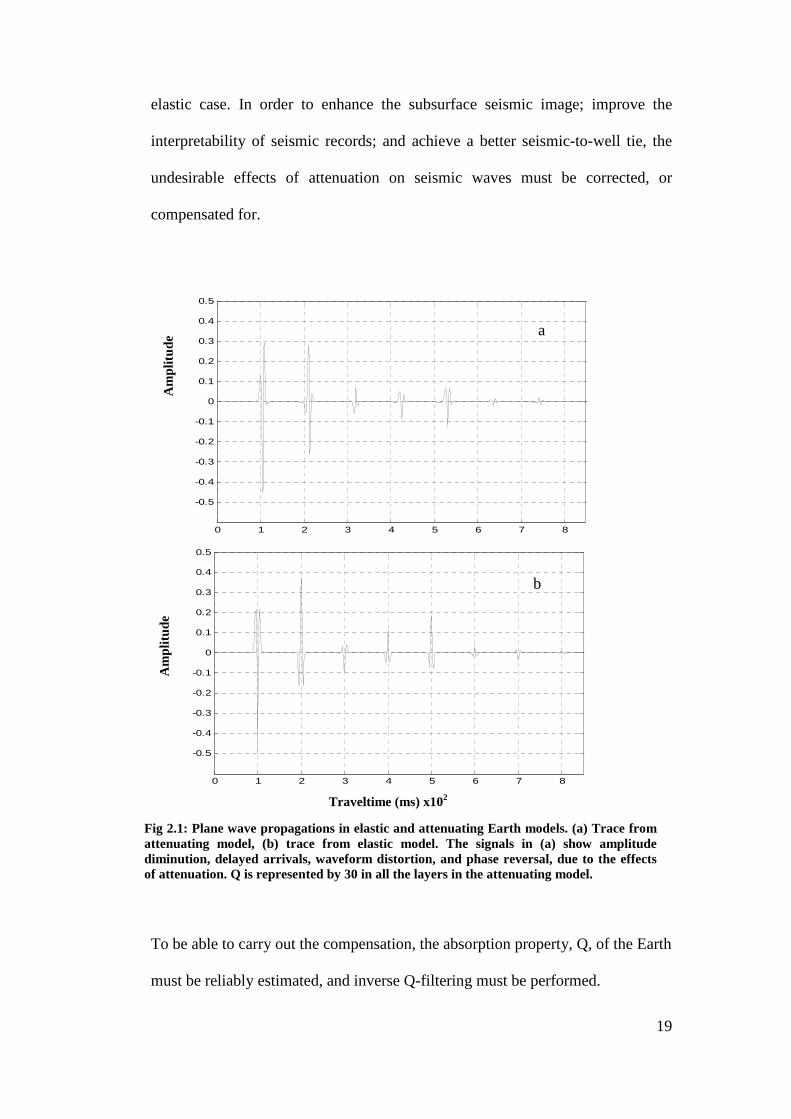
19
elastic case. In order to enhance the subsurface seismic image; improve the
interpretability of seismic records; and achieve a better seismic-to-well tie, the
undesirable effects of attenuation on seismic waves must be corrected, or
compensated for.
To be able to carry out the compensation, the absorption property, Q, of the Earth
must be reliably estimated, and inverse Q-filtering must be performed.
Fig 2.1: Plane wave propagations in elastic and attenuating Earth models. (a) Trace from attenuating model, (b) trace from elastic model. The signals in (a) show amplitude diminution, delayed arrivals, waveform distortion, and phase reversal, due to the effects of attenuation. Q is represented by 30 in all the layers in the attenuating model.
0 1 2 3 4 5 6 7 8
-0.5
-0.4
-0.3
-0.2
-0.1
0
0.1
0.2
0.3
0.4
0.5
0 1 2 3 4 5 6 7 8
-0.5
-0.4
-0.3
-0.2
-0.1
0
0.1
0.2
0.3
0.4
0.5
Traveltime (ms) x102
Am
plitu
de
Am
plitu
de
a
b
20
Q estimation in seismic data and attenuation compensation are the subjects of
chapters three and five respectively. A review of some existing techniques of Q
measurement is presented in the next section.
2.4: Review of techniques for Q measurement in seismic data
Reliable estimate of Q is required for correcting attenuation in seismic records.
Therefore, different techniques have been proposed for the measurement of
attenuation in seismic data. All measurement techniques are based on the
comparison of wave properties at two points, h� and h6 in the absorbing media.
The energy dissipation in waves due to attenuation can be defined as:
%&h6� %(&h��exp @.&-�. 2.14
Where %&h6� and %(&h�� are the signal at near and far positions, and . is the
coefficient of attenuation. Cheng et al. (1982) and Fink et al. (1983) measured
attenuation in full waveform sonic logs. Their findings show that a profile of
centroid frequencies gives reliable representation of full waveform sonic log
data, for correlating the attenuation and velocity of P- and S-waves. Goueygou et
al. (2002) measured attenuation in concrete using the spectral ratio technique.
They simulated ultrasonic signal through a concrete material of known
attenuation, and applied the cross spectrum technique to determine the average
Q. They concluded that multiple measurements of attenuation provide reliable
measurement of Q and reduce errors due to the presence of noise. Techniques of
Q measurement in seismic data can be classified into two: the time domain
method, and the frequency domain method (Tonn, 1991). An issue confronting
many of the Q measuring techniques is the extraction of a seismic wavelet.
Seismic wavelet extraction is easy in synthetic data but often difficult in real
21
seismic data due to spectral interference from noise and multiples. The problem
of spectral interference sometimes leads to negative Q values. The widely
accepted techniques for Q measurement in seismic data are reviewed in the next
paragraphs.
2.4.1: Wavelet modelling method
Introduced by Jannsen et al. (1985), the wavelet modelling technique for Q
measurement is based on a matching technique. A synthetic seismic pulse is
modelled and perturbed to match an observed attenuated seismic pulse in terms
of the spectral shape; the amplitude size; and the frequency content, by varying
the Q value used in the attenuation model for generating the synthetic wavelet:
ij&-, �j� � i�&-, ���, 2.15
�j � ��,
where i� is the observed seismic amplitude, and ij is the synthetic amplitude
spectral. The Q value used in the synthetic model is perturbed until a maximum
fit between the synthetic and real spectral is achieved. The Q value that produced
the maximum fit is assumed to be the real Q that is responsible for the
attenuation in the observed seismic signal. The comparison of a modelled and a
real seismic wavelet is based on a L1, or L2 norm. The L1 norm is the difference
in amplitude values (size) between the two signals while the L2 norm is the least
square misfit between the two amplitudes spectral (Tonn, 1991). The method is
reliable but computationally intensive and time consuming.

22
2.4.2: Rise time method
The method being among the earliest, was extensively used before computers
became widely used in seismology (Tonn, 1991). Introduced by Gladwin and
Stacy (1974), the rise time method is an empirical based method of Q
measurement. It is based on the observation that the seismic wavelet becomes
broadened as it travels from one point to another in an attenuating medium. As
the wavelet broaden, its rise time (k) changes. Rise time is the time between the
zero and maximum amplitude of a seismic pulse. The rise time of a seismic
wavelet at two different points in an attenuating medium can be related (Gladwin
and Stacy, 1974) as:
k k( P ] l ���H( m<, 2.16
where k( and k are the rise times at zero and time t, and ] is a constant.
Kjartanson (1979) showed that c is constant when Q is greater than or equal to
20, but varies when Q is less than 20. ] is dependent on the source, nature of the
rock, and the receiver (Gladwin and Stacy, 1974; Kjartanson, 1979; Muckelman,
1985; Tarif and Bourbie, 1989). Robust measurement of Q in field data using the
rise time method is difficult because c depends on factors that cannot be
determined during the measurement.
2.4.3: Analytical signal method
Q measurement using the analytical signal method is based on the ratio of the
instantaneous amplitude of the analytical signal at two positions in an attenuating
layer. The method was introduced by Engelhard (1986). An analytical signal in
this case is a measured seismic trace described by instantaneous amplitude,
frequency, and phase.
23
nQ Jo\&H�o"&H�K @ /p0&q�rs� P ], 2.17
where i� and i6 are the instantaneous amplitudes of the analytical signals at two
locations, k is the interval time, that is, the relative time of a data point within the
wavelet duration, p. r denotes the average over a ray path, 3 is the instantaneous
frequency calculated by taking the derivatives of the instantaneous phase with
respect to time, and t is the group traveltime. ] is a constant that represents
energy loss due to geometric spreading, and the reflection and transmission
process. The reliability of Q estimate from this method largely depends on t.
Slight error in T can cause significant error in Q (Sun, 2009). The basic
algorithm for the analytical signal method is similar to that of the spectral ratio
method, except that the former is a time domain method.
2.4.4: Spectral ratio method
The spectral ratio method was first described by Bath (1974). The method is
based on the ratio of amplitude or power of the transmitted to the incident
signals. Q is extracted from a plot of the ratio of amplitudes and frequency. The
method can be generally defined as:
nQ uo\&0,v\�o"&0,v"�w @ /0�$ &h6 @ h�� 2.18
Where i� and i6 are the respective amplitude spectrum of seismic signal at
distances h� and h6, 3 is the frequency and T is the velocity. The spectral ratio
method has been widely used for estimating attenuation, especially in vertical
seismic profile (VSP) data (Spencer et al., 1982; Tonn, 1991). Q estimates based
on this method are affected by a number of factors including source-receiver
coupling, scattering, thin layer effects, and geometric spreading. Q estimates
24
from spectral ratios are also sensitive to noise and the choice of frequency band.
Improvements to the classical spectral ratio method include the work of
Dasgupta and Clark (1998) and Rein et al. (2009b). Dasgupta and Clark (1998)
introduced a method to account for the variation of apparent attenuation with
offset. Rein et al. (2009b) presented a method to address the effects of source-
receiver directivity and attenuation anisotropy in the overburden materials.
Spectral interference and the choice of frequency bandwidth for the spectral ratio
are still issues in this method.
2.4.5: Frequency shift method
The frequency shift method is based on the fact that absorption is a high-
frequency filtering process – where the high frequency content of the seismic
wave is preferentially attenuated. The method compares the frequency content of
a seismic pulse at two different locations in the absorbing medium and estimates
Q from the difference in the frequency and traveltime of the two seismic signals
being compared. The method can be generally defined as:
]3� @ ]36 /0H� . 2.19
Where ]3� and ]36 are the frequency domain spectra of the signal at locations 1
and 2 respectively, 3 is the frequency and < is the traveltime. The frequency
content of a spectrum may be expressed by an average parameter (Quan and
Harris, 1997) or by a point in the spectrum (Zhang and Ulrych, 2002). To a first
order, Q estimate from this method is not affected by far field geometrical
spreading, transmission and reflection loss (Quan and Harris, 1997). This method
has been extensively applied for Q estimates in VSP and surface seismic data.

25
Accurate estimation of wavelet spectral in traces recorded from thin layers is still
a problem in the frequency shift method.
Among the techniques of Q measurement reviewed above, only the spectral ratio
and the frequency shift methods are currently being used for measuring
attenuation in seismic data. This is probably due to the fact that other methods
require many assumptions that are hard to quantify. In chapter three of this
thesis, a new algorithm based on centroid frequency shift is presented. The
choice of frequency shift method (Quan and Harris, 1997) is based on the fact
that the centroid frequency, an average spectral parameter is less affected by
interference from noise and other forms of signal corruption.
2.5: Mechanisms of seismic attenuation
Q Model or mechanism of attenuation explains how different rock properties and
physical process are linked to the phenomenon of seismic attenuation. Although
several mechanisms have been put forward to explain the phenomenon of
seismic energy loss in Earth media, there is no agreement or consensus in the
scientific community on which model is superior to the other. Due to the spatial
and temporal changes in the Earth layers, a model that best suits a rock type or an
environmental setting may fail in another rock type or a different geological
setting. Therefore, there is no single model that can describe attenuation in all
rock types and environmental settings. This section of the thesis focuses on
mechanisms of intrinsic attenuation in partially or fully saturated porous rocks
that are typical for hydrocarbon reservoirs. Most of the mechanisms describing
26
intrinsic attenuation in reservoir rocks consider two processes: (i) sliding
frictional movement among rock grains, and along the grain matrix contact
during the passage of seismic waves; and (ii) oscillatory fluid flow in and out of
rock pore spaces during the passage of seismic waves. Either or both of these
processes cause part of the energy of a travelling wave to be irreversibly lost.
Often mentioned attenuation mechanisms include thermo-elasticity (Ricker,
1977; Aki and Richard, 1980), gas bubble model (White, 1975), squirt flow
model (Mavko and Jizba, 1991), fractal-pore model (Brajanovski et al., 2005;
Brajanovski et al., 2006), patchy saturation model (Norris, 1993; Muller and
Gurevich, 2004), and wave induced fluid flow (Pride et al., 2004). Below, I
review the mechanisms of attenuation that are commonly referenced in literature
dealing with attenuation.
2.5.1: Squirt flow mechanism
The squirt flow mechanism explains seismic attenuation in terms of the frictional
force due to the pressure induced fluid flow between the compliant pores and the
stiffened parts of the rock. The passage of waves induces variation of pore
pressure between the compliant pores and the stiff part of the rock, causing fluid
flow from the compliant pores into the stiff part. During the fluid flow, some
energy of the waves is converted into heat, thus causing attenuation of the waves’
energy. An example of a compliant pore is a soft, thin crack, or fracture, or
micro-cracks which is closed under high pressure (Dvorkin et al., 1995). The
presence of micro-cracks in a rock influences the strength and elastic response of
the rock (Heap and Faulkner, 2008). The stiff parts of the rock are the primary
pore structures that do not close under high pressure. The attenuation process is
27
frequency dependent. The frequency involved is classified into three: (i) low
frequency, usually referred to as the “relaxed” state; (ii) high frequency, usually
referred to as the “unrelaxed” state; and (iii) the transition frequency. At low
frequencies, the pressure equilibrates and the pore pressure is quasi-static.
Attenuation is insignificant and seismic velocities approach their low frequency
limit predicted by Gassmann’s (1951) equation. At high frequency, the fluid is
“unrelaxed”, attenuation is insignificant and seismic velocities approach their
high frequency limit. At the transition frequencies, the intensive fluid cross-flow
between the compliant and stiff parts results in significant seismic attenuation
and velocity dispersion. The transition frequency is referred to as ‘squirt flow
frequency’. The squirt flow frequency is proportional to the permeability of the
rock and inversely proportional to the viscosity of the saturating fluid (Chapman
et al., 2003). The squirt flow mechanism is based on the Biot (1956a & b) model.
The basic assumptions in the squirt flow model are: the rock is isotropic,
macroscopically homogeneous, and the pores are arbitrarily shaped and
randomly distributed.
Understanding the squirt flow mechanism is important for the interpretation of
laboratory rock physics measurements. Hudson et al. (1996) and Van der Kolk et
al. (2001) have proposed models for the influence of squirt flow on anisotropic
seismic response of fractured in-situ rocks. The Biot-Squirt model (BISQ)
proposed by Dvorkin et al. (1995) incorporates the Biot and the Squirt models to
link compressional wave velocity and attenuation to the elastic constant of a
drained rock skeleton. The elastic constant depends on the squirt flow length (n), and the rock and fluid properties (e.g., porosity, permeability, saturation,
28
viscosity, and compressibility). The Biot-Squirt model, compared with the Biot
model, provides better description of attenuation and velocity dispersion that is
commonly observed in porous rocks.
2.5.2: Wave induced fluid flow in random porous media
This model explains attenuation in terms of the frictional movement of fluids in
and out of the pore structures of a heterogeneous rock, due to the pressure
induced by the passing waves (Muller and Gurevich, 2005a). The inhomo-
geneous rock consists of numerous clusters with random porosity. Each cluster
consists of different minerals which have different elastic moduli, but have
comparable sizes and similar density (x); porosity (y); and permeability (C). The
movement of seismic energy through such rock creates variation of pore
pressure, and thus leads to fluid flow among the clusters. The frictional
movement during the fluid flow causes attenuation of the energy of passing
waves. At low frequencies, pressure attains equilibrium, attenuation is
insignificant and seismic velocities approach their low frequency limits predicted
by Gassmann’s (1951) relation. At high frequencies, pressure could not attain
equilibrium and attenuation is insignificant. At intermediate frequencies,
macroscopic fluid flow is induced and friction occurs at the clusters. These result
in significant attenuation and velocity dispersion.
The basic assumptions of this model are: (i) the scale of heterogeneity (L) is
mesoscopic, i.e. smaller than the wavelength (9) but larger than the individual
pore size; (ii) pores are distributed randomly, and pore shapes are arbitrary; (iii)
heterogeneity in the rock is spatially random. Muller and Gurevich (2005a & b)
29
explained that when a rock model described above is saturated with fluid and
loaded with seismic waves, the overall seismic attenuation in the rock is the
average of the attenuation in the individual clusters in the rock. Mathematical
models put forward to explain this model include Dvorkin and Nur (1993) and
Pride and Berryman (2003).
2.5.3: Patchy saturation model
Unlike the squirt flow and the random porous models that deal with rocks
saturated with one type of fluid, the patchy saturation model deals with
heterogeneous rock bodies saturated with two or three different types of fluids
concentrated in patches and their surrounding regions. The patches are
mesoscopic, and larger than a typical pore size, but small compared to a seismic
wavelength. The pore fluids are assumed to be immiscible. This rock model
perfectly captures hydrocarbon reservoirs that often contain water, gas, and oil.
In this model, seismic wave attenuation is explained by wave induced fluid flow
between patches and surrounding rock. During the flow, the energy of the
travelling wave is converted to heat. Elastic waves travelling through such rocks
show characteristic frequency dependent attenuation and velocity dispersion
(Dvorkin et al., 2003). Attenuation is insignificant at low frequency (‘relaxed’
state) and velocity at the low frequency limit is estimated using the Gassmann’s
(1951) relation. At intermediate frequencies, attenuation and velocity dispersion
arise from induced fluid flow between the fully water saturated patches and the
partially gas saturated region. In the intermediate frequency range, attenuation
and dispersion are significant. At high frequencies, the patch is said to be
30
‘unrelaxed’, seismic velocity approaches the high frequency limit and attenuation
is insignificant (Mavko and Dvorkin, 2005).
Patchy saturation is believed to be a major cause of dispersion and attenuation in
the seismic exploration frequency range (Pride et al., 2004). White (1975) and
Noris (1993) are among the first theoretical models for wave attenuation in
patchy saturated rock. Theoretical models proposed for randomly distributed
fluid in patches include Muller and Gurevich (2004) and Tom et al. (2007). The
models show that attenuation increases with frequency and porosity, whilst
velocity increases with frequency, it decreases with porosity. The basic
assumption in their model is that fluid is randomly spatially distributed. Krzikalla
et al. (2006) numerically simulated wave propagation in a partially saturated
rock model containing water with gas inclusions. They extracted attenuation
from the simulated seismograms using a finite difference algorithm developed
by Wang (2001), and they inferred the size of the patch from the estimated
attenuation. The work by Krzikalla et al. (2006) suggests the possibility of
estimating the size of a fluid patch from seismic data.
2.5.4: Porous – Fracture model
Different from the above three models which considered only porous (but not
fractured) media, the fracture–porous model considers the mechanism of
attenuation in porous and fractured Earth media. This model is important in
exploration geophysics as hydrocarbon reservoirs are often naturally fractured,
and the fractures control the secondary permeability of the reservoir. The fracture
– porous model explains seismic attenuation and velocity dispersion in terms of
31
the energy loss in seismic waves due to the fluid flow between the pores and
fractures of a rock. Based on Biot’s theory of poroelasticity (Biot,1956a) and
Norris (1993), Brajanovski et al. (2006) studied attenuation by modelling
randomly oriented fractures in highly porous thin layers in a porous background
rock. They assumed that the porous media is permeated by a periodic sequence
of fractures. The study shows that: (i) when pores and fractures are dry, the rock
behaviour is similar to that of a dry, isotropic, and porous material with linear-
slip interfaces; (ii) and when rock pores and fractures are saturated with liquid,
the rock exhibits significant attenuation and velocity dispersion due to the
induced fluid flow between the pores and the fractures. Brajanovski et al. (2006)
show that the magnitude of attenuation is dependent on the degree of fracturing
and the background porosity of the media.
Similar to all other models, attenuation and velocity dispersion in a fracture –
porous model is frequency dependent. Attenuation is insignificant at high and
low frequencies but significant at intermediate frequency. According to this
model, the characteristic frequency of attenuation and dispersion depends on the
background permeability, fluid viscosity, and fracture density (Brajanovski et al.,
2005; Brajanovski et al., 2006; Hall et al., 2008; Al-Harrasi et al., 2011). Fracture
size in sedimentary settings may vary from micro-scale to macro-scale. The
macro-scale fractures control the reservoir storability and fluid flow (Al-Harrasi
et al., 2011). Observations from indirect data sources (e.g., seismicity) from fault
related fluid flow can be used to explain the process of fluid flow in natural faults
at depths and scales that are not available to laboratory experiements (Faulkner et
al., 2010). Using space concentration of penny-shaped cracks in porous matrix,
32
Hudson et al. (1996) and Chapman et al. (2003) proposed theoretical models for
attenuation and dispersion in porous-fractured media. The basic assumptions of
the porous–fracture model are: (i) the direction of propagation of waves in the
rock is perpendicular to the orientation of the fractures; (ii) the porous
background without fractures is isotropic; and (iii) the fractures are periodic and
parallel to the wave direction.
2.6: Modulus – Frequency – Dispersion
Consensus among the mechanisms of attenuation are: (i) the passage of seismic
waves in a saturated porous rock causes variation in pore pressure between the
different regions of the rock; (ii) attenuation and dispersion are frequency
dependent; and (iii) attenuation is significant at the intermediate frequency range,
but insignificant at the extreme frequencies. The change in the rock modulus due
to the frequency of a propagating wave is the subject of this section. The section
reviews some rock physics formulations for measuring rock elastic modulus at
high and low frequencies, and for measuring attenuation or inverse quality factor
as the difference between high and low frequency moduli. The rock model
selected for this study consists of two grain sizes: the clay size; and the sand size.
The clay size materials are formed in clusters or patches and the patches are
assumed to be fully water saturated. The sand-size grains (i.e., the larger
particles) form the background rock, and are partially saturated with gas. The
rock model is shown in figure 2.2. Although the Gassmann (1951) and Mavko et
al. (1998) equations are the principal tools for this study, this section will follow
the report by Walls et al. (2006) to introduce the main concepts. In this section,
33
dry rock is used to capture partially gas-saturated rock; wet rock is used to
capture fully water-saturated rock; and inverse quality factor (���) is used
interchangeably with attenuation.
The propagation of seismic waves in a rock model described above would cause
difference in pore pressure of the fully saturated patches and the partially
saturated regions. The differential pore pressure will lead to oscillatory fluid flow
between the patches and the surrounding region. During the fluid flow, a part of
the energy of the passing wave is converted to heat, and seismic attenuation
arises. The flow effect determines the changes in the elastic moduli of the rock
with frequency (Mavko and Dvorkin, 2005). The changes in elastic modulus are
related to attenuation via the Krammer-Kronig relation (Mavko et al., 1998).
The elastic modulus, z is linked to frequency, 3, according to the standard linear
solid model (Zener, 1948; Mavko et al, 1998) as:
z&0� {I{|}�~& �����\�{|~{I& �����\ , 2.20
where z( and z� are the high and low frequency elastic moduli, respectively.
3�� is the critical frequency at which transition between low frequency and high
frequency occurs. “The reaction of a rock with patchy saturation to loading due
to wave propagation depends on the frequency of the wave. If the frequency is
low, loading of the rock is slow, the oscillatory fluid flow between the fully
water-saturated patch and the partially gas-saturated region next to it equilibrates,
and the patch is said to be ‘relaxed’. Conversely, if the frequency is high, loading
of the rock is fast, the resulting oscillatory pressure between the fully water-
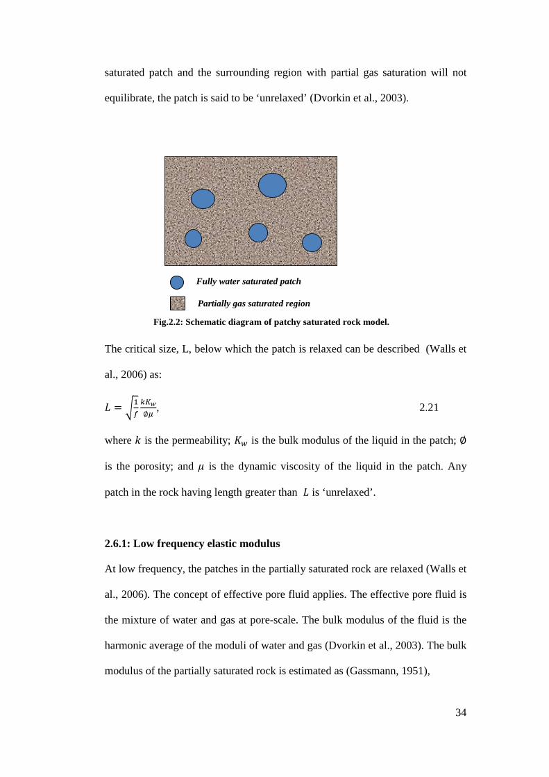
34
saturated patch and the surrounding region with partial gas saturation will not
equilibrate, the patch is said to be ‘unrelaxed’ (Dvorkin et al., 2003).
The critical size, L, below which the patch is relaxed can be described (Walls et
al., 2006) as:
� ��0 ��Vy� , 2.21
where C is the permeability; �+ is the bulk modulus of the liquid in the patch; y
is the porosity; and � is the dynamic viscosity of the liquid in the patch. Any
patch in the rock having length greater than � is ‘unrelaxed’.
2.6.1: Low frequency elastic modulus
At low frequency, the patches in the partially saturated rock are relaxed (Walls et
al., 2006). The concept of effective pore fluid applies. The effective pore fluid is
the mixture of water and gas at pore-scale. The bulk modulus of the fluid is the
harmonic average of the moduli of water and gas (Dvorkin et al., 2003). The bulk
modulus of the partially saturated rock is estimated as (Gassmann, 1951),
Fully water saturated patch
Partially gas saturated region
Fig.2.2: Schematic diagram of patchy saturated rock model.

35
�joH( �j y��_��&�~y�����_� �#⁄ ~��&��y���~y�#�����_� �#⁄ , and 2.22
��� ���� P ������ . 2.23
Where �� is the bulk modulus of the mineral phase (i.e., clay and quartz); ���� is
the bulk modulus of the dry rock; �� is water saturation; �� is the modulus of
water; and �� is the modulus of gas. The compressional modulus at low
frequency (zjoH() is defined in terms of bulk modulus (�joH() and shear modulus
(����) as:
zjoH( ��joH( P �� ����. 2.24
Similarly, the low frequency compressional moduli can be estimated directly
using the approximate Vp- only substitution equation (Mavko et al., 1998):
zjoH( zj y{����&�~y���{��� {#⁄ ~��&��y���~y{#���{��� {#⁄ . 2.25
While all other terms remain the same as defined above, z represents the
compressional modulus.
2.6.2: High frequency elastic modulus
At high frequency compressional modulus, fluid distribution is at patch scale,
and the concept of effective pore fluid is not applicable. The bulk modulus of the
fully-water saturated patch, �� and the bulk modulus of the partially gas-
saturated region, ����( is estimated individually using the Gassmannn (1951)
equation. The compressional modulus of the entire rock is estimated as the
harmonic average of the water and gas-saturated regions of the rock. Assuming
that the shear modulus is the same for water saturated and gas-saturated regions,
the compressional modulus of the entire rock is calculated in terms of the bulk
and shear modulus (Walls et al., 2006) as:

36
�{���| ��� ~����_� P �����#� ¡~����_�, 2.26
where �� is the volumetric concentration of the fully water saturated patch,
1 @ ¢+ is the volumetric concentration of the partially gas saturated region. The
bulk modulus of the fully-water saturated patches (��) is:
�� �j y�����&�~y������� �#⁄ ~��&��y���~y�#������� �#⁄ , 2.27
and the bulk modulus of the gas-saturated region (����£) is:
����£ �j y�����&�~y������� �#⁄ ~��&��y���~y�#������� �#⁄ . 2.28
Using a similar approach, the compressional modulus of the entire rock at high
frequency (zjoH�) can be estimated using the approximate Vp-only substitution
equation (Mavko et al., 1998):
�{���| ��{ P ����{#� ¡ , where 2.29
z� zj y{����&�~y���{��� {#⁄ ~��&��y���~y{#���{��� {#⁄ , and 2.30
z���£ zj y{����&�~y���{��� {#⁄ ~��&��y���~y{#���{��� {#⁄ . 2.31
For a reservoir rock model with porosity, clay content, dry frame bulk modulus,
and shear moduli of 0.27, 0.10, 2.64 GPa, and 3.2 Gpa, respectively, the
estimated compressional moduli of the rock are plotted in figures 2.3 and 2.4.
The compressional moduli plotted in figure 2.3 are estimated using the
Gassmannn’s (1951) equation, while those plotted in figure 2.4 are estimated
using the Vp-only substitution equation of Mavko et al. (1998).
An important observation from the plots is that fluid heterogeneity is a necessary
condition for attenuation. The observed difference between the low and the high
frequency moduli for dry (0% �� or 100% ��) and fully water saturated rock
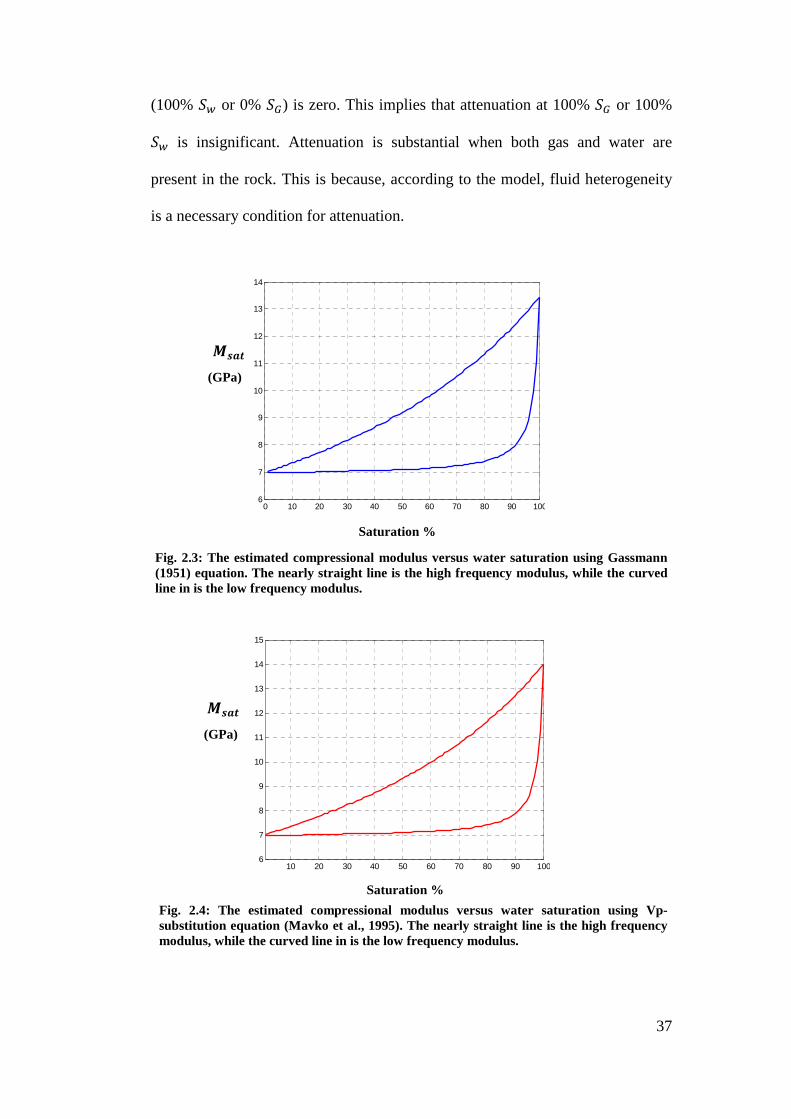
37
0 10 20 30 40 50 60 70 80 90 1006
7
8
9
10
11
12
13
14
Msa
t
water sat. %
10 20 30 40 50 60 70 80 90 1006
7
8
9
10
11
12
13
14
15
(100% �+ or 0% ��) is zero. This implies that attenuation at 100% �� or 100%
�+ is insignificant. Attenuation is substantial when both gas and water are
present in the rock. This is because, according to the model, fluid heterogeneity
is a necessary condition for attenuation.
Fig. 2.4: The estimated compressional modulus versus water saturation using Vp-substitution equation (Mavko et al., 1995). The nearly straight line is the high frequency modulus, while the curved line in is the low frequency modulus.
Saturation %
Saturation %
¤¥¦§ (GPa)
¤¥¦§ (GPa)
Fig. 2.3: The estimated compressional modulus versus water saturation using Gassmann (1951) equation. The nearly straight line is the high frequency modulus, while the curved line in is the low frequency modulus.

38
2.6.3: Estimating inverse quality factor (̈ ��� from modulus-frequency-
dispersion
Change in the rock modulus due to a change in frequency is referred to as
modulus-frequency-dispersion. The estimated difference between the high and
low frequency modulus can be translated into attenuation using the standard
linear model (Zener, 1948; Mavko et al., 1998), if we assume that the rock is
viscoelastic and linearly frequency dependent. The maximum inverse quality
factor (��o,�� ) can be estimated from the modulus-frequency-dispersion (Mavko
et al., 1998) as:
��o,�� {|�{¡6©{¡{|, 2.32
where z� is the high frequency compressional modulus, and zª is the low
frequency
compressional modulus. In figures 2.5, the red plot is the inverse quality factor
estimated using the Gassmann (1951) relation, while the blue plot is the inverse
quality factor estimated using the Mavko et al. (1998) equation. The MATLAB
codes written to compute the inverse quality factor (��o,�� ) as a function of
saturation are given in appendices 2B and 2C, respectively. The model discussed
above will be applied in chapter four to estimate P-wave and S-wave inverse
quality factor from well log data recorded in the Gullfaks field.
2.6.4: Irreducible water saturation, «¬®®
Real hydrocarbon reservoirs usually contain irreducible water saturation in
addition to the oil or/and gas. Irreducible water saturation is the portion of the
pore space occupied by water at maximum hydrocarbon saturation (Crain Ross,
2000). This water is immobile and cannot be displaced, no matter how highly
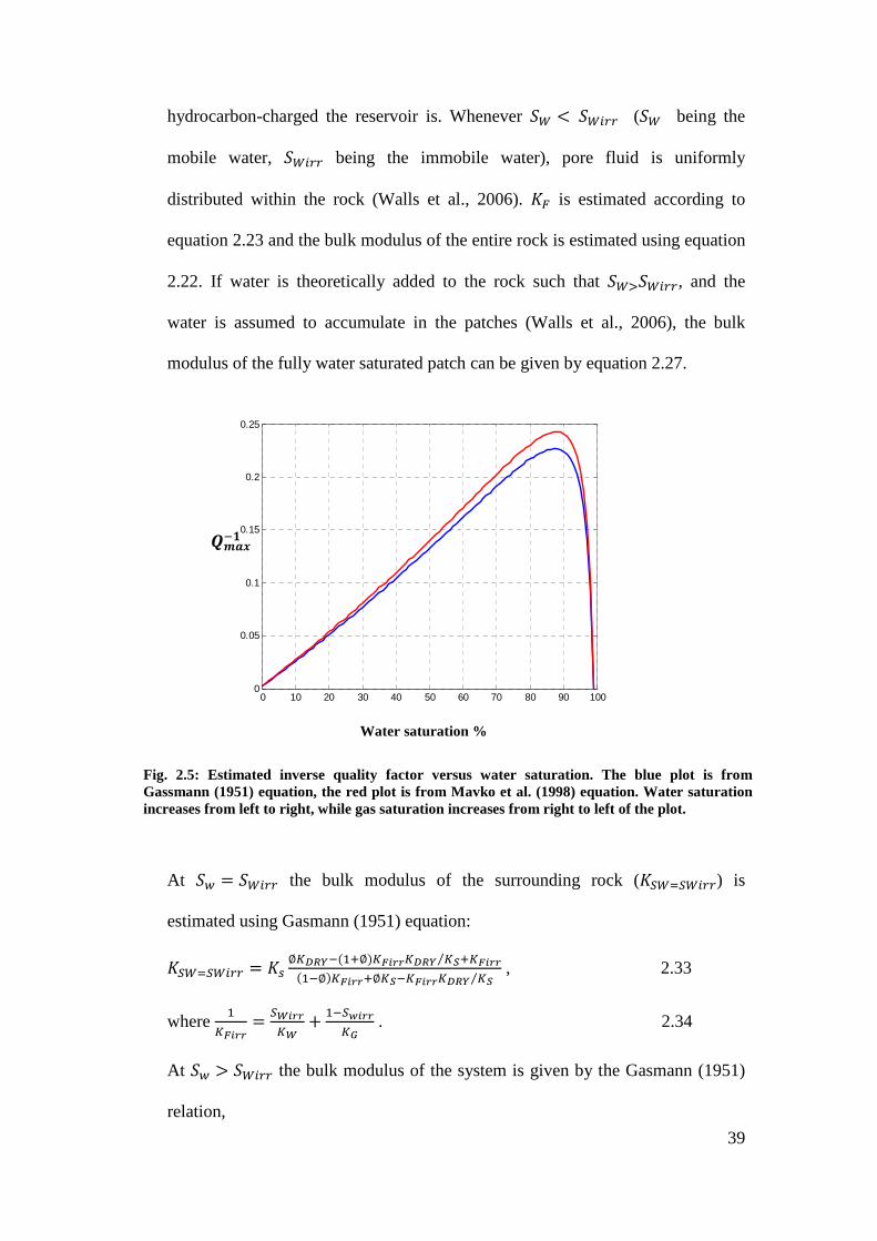
39
hydrocarbon-charged the reservoir is. Whenever �� ¯ ����� (�� being the
mobile water, ����� being the immobile water), pore fluid is uniformly
distributed within the rock (Walls et al., 2006). �° is estimated according to
equation 2.23 and the bulk modulus of the entire rock is estimated using equation
2.22. If water is theoretically added to the rock such that ��±�����, and the
water is assumed to accumulate in the patches (Walls et al., 2006), the bulk
modulus of the fully water saturated patch can be given by equation 2.27.
At �+ ����� the bulk modulus of the surrounding rock (���������) is
estimated using Gasmann (1951) equation:
��������� �j y�����&�~y���²__���� �#⁄ ~��²__&��y���²__~y�#���²__���� �#⁄ , 2.33
where ���²__ ��²__�� P ���V²__�� . 2.34
At �+ ³ ����� the bulk modulus of the system is given by the Gasmann (1951)
relation,
0 10 20 30 40 50 60 70 80 90 1000
0.05
0.1
0.15
0.2
0.25
¨´¦µ��
Water saturation %
Fig. 2.5: Estimated inverse quality factor versus water saturation. The blue plot is from Gassmann (1951) equation, the red plot is from Mavko et al. (1998) equation. Water saturation increases from left to right, while gas saturation increases from right to left of the plot.
40
�� #¶·¸__|~����_� 0 � ~����_� P ��0¹�#� #�¸__~����_�, 2.35
where 3O ��!#�¸__����¸__ , and 2.36
�� #¶·¸__|~����_� &�����¸__� &����¸__�⁄� ~����_� P &����� &����¸__�⁄�#� #�¸__~����_�. 2.37
Following a similar procedure and assumptions, the Vp-only substitution
equation of Mavko et al. (1998) can be applied to estimate compressional
modulus of the rock. When �+ º �����, the compressional modulus at
irreducible water saturation, z�»sL��£ is estimated according to equations 2.23
and 2.25. For a condition of �+ ³ �����, the compressional modulus of the rock
is estimated as:
�{#¶·¸__| &�����¸__� &����¸__�⁄{ P &����� &����¸__�⁄{#� #�¸__ , 2.38
where z� is from equation 2.30, and
z�����L�� zj y{�_��&�~y���¸__{�_� {#⁄ ~��¸__&��y���¸__~y{#���¸__{�_� {#⁄ . 2.39
�°L�� is defined in equation 2.34. The effect of the irreducible water saturation
on the maximum inverse quality factor (��o,�� ) are shown in figures 2.6 and 2.7.
The MATLAB codes written to show the effects of irreducible water saturation
on the estimated inverse quality factor, ��o,�� are shown in appendices 2D and 2E
respectively. An important observation from the effect of irreducible water
saturation on attenuation (Figs. 2.6 and 2.7) is that the higher the irreducible
water saturation, the lower the attenuation. The observation can be explained
thus: the higher the irreducible water saturation, the less the pore spaces, or the
pore volume that is available to accommodate mobile water and gas; the pore
fluid-mix is therefore dominated by a particular fluid (i.e., the irreducible water);

41
and fluid heterogeneity, a condition necessary for attenuation according to the
patchy saturation model is insignificant, and thus attenuation is insignificant.
10 20 30 40 50 60 70 80 90 1000
0.05
0.1
0.15
0.2
0.25
water sat. %
10 20 30 40 50 60 70 80 90 1000
0.05
0.1
0.15
0.2
0.25
Saturation %
Fig. 2.6: The estimated maximum inverse quality factor versus saturation at 40%, and 80% irreducible water saturation, using Gassmann (1951) equation. The higher the irreducible water saturation, the lower the attenuation.
¨´¦µ��
Fig. 2.7: The estimated maximum inverse quality factor versus saturation at 40%, and 80% irreducible water saturation, using Mavko et al. (1998) equation. The higher the irreducible water saturation, the lower the attenuation.
Saturation %
¨´¦µ��
42
Chapter Three
DETERMINATION OF QUALITY FACTOR (Q) IN REFLECTION
SEISMIC DATA
43
3.1: Abstract
A new method for measuring attenuation in reflection seismic data is presented.
The inversion process involves two key stages: computation of the centroid
frequency for the individual signal using variable window length and fast Fourier
transform; and estimation of the difference in the centroid frequencies and
traveltimes of paired incident and transmitted signal. The method introduces a
shape factor, a constant which allows several spectral shapes to be used to
represent a real seismic signal without altering the mathematical model.
Application of the method to synthetic data shows that it can provide reliable
estimates of Q using any of the spectral shapes commonly assumed for real
seismic signals. Tested against two published methods of Q measurement, the
new method shows less sensitivity to interference from noise and change of
frequency bandwidth. The method is also applied to a 3D data set from the
Gullfaks field, North Sea, Norway. The mean attenuation (1/��) calculated from
500 measurements at intervals AB, BC, CD, and DE, are 0.0196, 0.0573, 0.0389,
and 0.0220, respectively. The 1/Q measured in a stack of the traces along CDP
602 line, qualitatively agrees with the 1/��. All the measurements show that
interval AB has the lowest 1/Q value, and that interval BC has the highest 1/Q
value. The values of 1/Q measured in the CDP stack using the new method are
consistent with those measured using the classical spectral ratio method. Because
of the strategic importance of the intrinsic attenuation to saturation and other
material properties of rocks, a procedure for quantifying the relative contribution
of the intrinsic attenuation in the composite attenuation measured in field seismic
data is presented. For interval DE, the value of intrinsic attenuation is 0.0138.

44
3.2: Introduction
Detailed knowledge of the attenuation structure of the Earth is essential for
hydrocarbon exploration. Studies on the anelastic properties of rocks have linked
attenuation to the presence of hydrocarbon and the saturation condition of rocks.
Laboratory experiments and mathematical models (Gassmann, 1951; Toksoz et
al., 1979; Winkler and Nur, 1979; Johnson and Toksoz, 1980; Klimentos and
McCann, 1990; Klimentos, 1995) have shown that attenuation can indicate
pressure, porosity, fluid type, and saturation level. Field studies also have shown
that attenuation can be used for lithology discrimination (Stainsby and
Worthington, 1985; Dasgupta and Clark, 1998; Singleton, 2008) and anisotropy
study of fractures (Helffrich et al., 2002; Maultzsch et al., 2007; Zhu et al., 2007;
Behura and Tsvankin, 2009; Clark et al., 2009; Al-Harrasi et al., 2011). In fact,
the study by Winkler and Nur (1979) indicates that attenuation (���) may be
more sensitive to the changes in saturation and pressure than the velocity. Apart
from its use in seismic data processing, the knowledge of attenuation is also
useful in seismic acquisition design. It helps in the survey planning stage to know
the portion of the source energy that will reach the target layers (Rickett, 2006).
Despite its numerous potential applications, attenuation analysis of seismic
reflection amplitudes is yet to become a routine in hydrocarbon industry. A lack
of reliable method for estimating seismic attenuation in field data was cited at the
2005 SEG (Society of Exploration Geophysicists) Development and Production
Forum as being the major limitation to the further development of ���
technology for hydrocarbon exploration. Another limitation in the use of ��� for
hydrocarbon exploration is how to determine the portion of ��� that is solely due
45
to the rock anelastic properties (e.g. saturation). This is because the ���
measured in seismic data is a combination of intrinsic attenuation, ��MH�� and
extrinsic (or scattering) attenuation, �8,H�� . The attenuation measured in field
seismic data is sometimes known as composite attenuation, �NO��. The three
elements can be related (Dainty, 1981; Richard and Menke, 1983) as:
1/�NO = 1/��MH + 1/�8,H 3.1
The extrinsic attenuation includes attenuation due to stratigraphic scattering (the
geometric arrangement of layers) and thin layering effects.
Attenuation is commonly measured in terms of the rock quality factor (�). The
inverse of the rock quality factor (���) is proportional to the attenuation
coefficient (.�as:
.&-� ��&+� /01&+�. 3.2
Where 3 is the frequency of the wave, and 2 is the velocity. During propagation,
the amplitude of a seismic wave decays, the peak frequency shifts towards the
lower frequency band and the wavelet width broadens. Methods proposed for �
measurement are based on the attenuation-induced changes in spectral properties
of seismic wavelets. Methods for determining � in seismic records include the
spectral ratio method (Bath, 1974; Spencer et al., 1982), centroid frequency-shift
method (Quan and Harris, 1997; Raji and Rietbrock, 2010) and peak frequency-
shift method (Zhang and Ulrych, 2002). The spectral ratio and the centroid
frequency-shift methods are design for Q measurements in VSP data. While
these methods provide robust Q estimates in VSP data, they are less successful
for estimating Q in reflection seismic data because of the strong influence of
46
reflections from closely spaced rock layers (Parra et al., 2006). Further to this,
the Q estimates provided by VSP data does not give areal coverage for the
attenuation properties in rocks. Improvements to the classic spectral ratio method
include the work of Dasgupta and Clerk (1998) and Rein et al. (2012a & b) .
Dasgupta and Clerk (1998) improved the accuracy of Q estimates from spectral
ratio method by estimating Q in the pre-stack domain- avoiding spectral
distortion due to stacking and the normal move out (NMO) stretch. Rein et al.
(2012a & b) improved Q estimates from the spectral ratio method by accounting
for the effects of source-receiver directivity, overburden anisotropy, and ray path
differences. However, the choice of frequency bandwidth for the spectral ratio is
still an issue in this approach. Although the peak frequency shift method (Zhang
and Ulrych, 2002) is designed for reflection seismic data, the technique largely
depends on the peak frequency. The peak frequency of a seismic signal– the
frequency that corresponds to the amplitude maxima– is easily influenced by a
number of factors including the presence of noise, inter-bed multiples, and the
wavelet extraction (windowing) process. These factors in turn affect the accuracy
of Q estimates using the peak frequency shift method.
The method presented in this chapter uses the centroid frequency. The centroid
frequency is similar to a statistical average of the frequencies in the spectrum of a
seismic signal (Barnes, 1993); it is more stable and less sensitive to interference
compared to the peak frequency. In all the frequency-shift based attenuation
methods, the shape of the seismic signal is commonly model. This is to allow for
the quantitative assessment of the attenuation-induced variation in the frequency
content of the seismic spectrum. The commonly assumed shapes include
47
Gaussian, boxcar, triangle (Quan and Harris, 1997), and Ricker (Zhang and
Ulrych, 2002). Arising from these shapes, different mathematical models are
defined for the various methods due to the differences in the spectral shapes (see,
Quan and Harris, 1997; Zhang and Ulrych, 2002). The model being presented in
this chapter uses a new mathematical relation, and a shape factor to measure � in
seismic records. The process of Q measurement can be divided into two parts:
computation of the centroid frequency for the individual signal using variable
window length and fast Fourier transform; and estimation of the difference in the
centroid frequencies and traveltimes of paired incident and transmitted signals.
The use of variable window length reduces interference from seismic multiples
and noise. The inclusion of a shape factor in the mathematical model allows the
users to represent the real seismic signal with any spectral shape that satisfies the
basic characteristics of a seismic signal (as commonly done in attenuation
measurement experiments) without altering the mathematical model. The
spectral shapes considered in the new attenuation model include Gaussian,
Ormsby (or boxcar), Ricker, and triangle wavelets.
In the following sections, I describe the proposed method and test it on synthetic
seismic records computed from various Earth Q models. The method is also
tested for Q measurement in field data recorded in the Gullfaks field, North Sea,
Norway. Following these, a method of quantifying the relative contribution of
the intrinsic attenuation in the composite attenuation measured in field seismic
data is discussed.
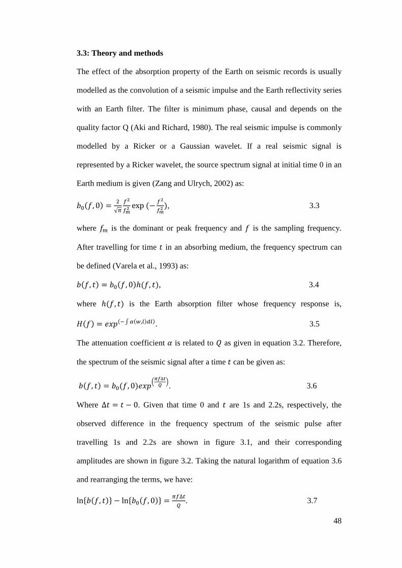
48
3.3: Theory and methods
The effect of the absorption property of the Earth on seismic records is usually
modelled as the convolution of a seismic impulse and the Earth reflectivity series
with an Earth filter. The filter is minimum phase, causal and depends on the
quality factor Q (Aki and Richard, 1980). The real seismic impulse is commonly
modelled by a Ricker or a Gaussian wavelet. If a real seismic signal is
represented by a Ricker wavelet, the source spectrum signal at initial time 0 in an
Earth medium is given (Zang and Ulrych, 2002) as:
%(&3, 0� 6√/ 0\0½\ exp &@ 0\0½\ �, 3.3
where 3� is the dominant or peak frequency and 3 is the sampling frequency.
After travelling for time < in an absorbing medium, the frequency spectrum can
be defined (Varela et al., 1993) as:
%&3, <� %(&3, 0�¾&3, <�, 3.4
where ¾&3, <� is the Earth absorption filter whose frequency response is,
¿&3� )'À&� l *&+,Á��Á�. 3.5
The attenuation coefficient . is related to � as given in equation 3.2. Therefore,
the spectrum of the seismic signal after a time < can be given as:
%&3, <� %(&3, 0�)'ÀJÂ�∆�à K. 3.6
Where ∆< < @ 0. Given that time 0 and < are 1s and 2.2s, respectively, the
observed difference in the frequency spectrum of the seismic pulse after
travelling 1s and 2.2s are shown in figure 3.1, and their corresponding
amplitudes are shown in figure 3.2. Taking the natural logarithm of equation 3.6
and rearranging the terms, we have:
lnÄ%&3, <�Å @ lnÄ%(&3, 0�Å /0∆H� . 3.7
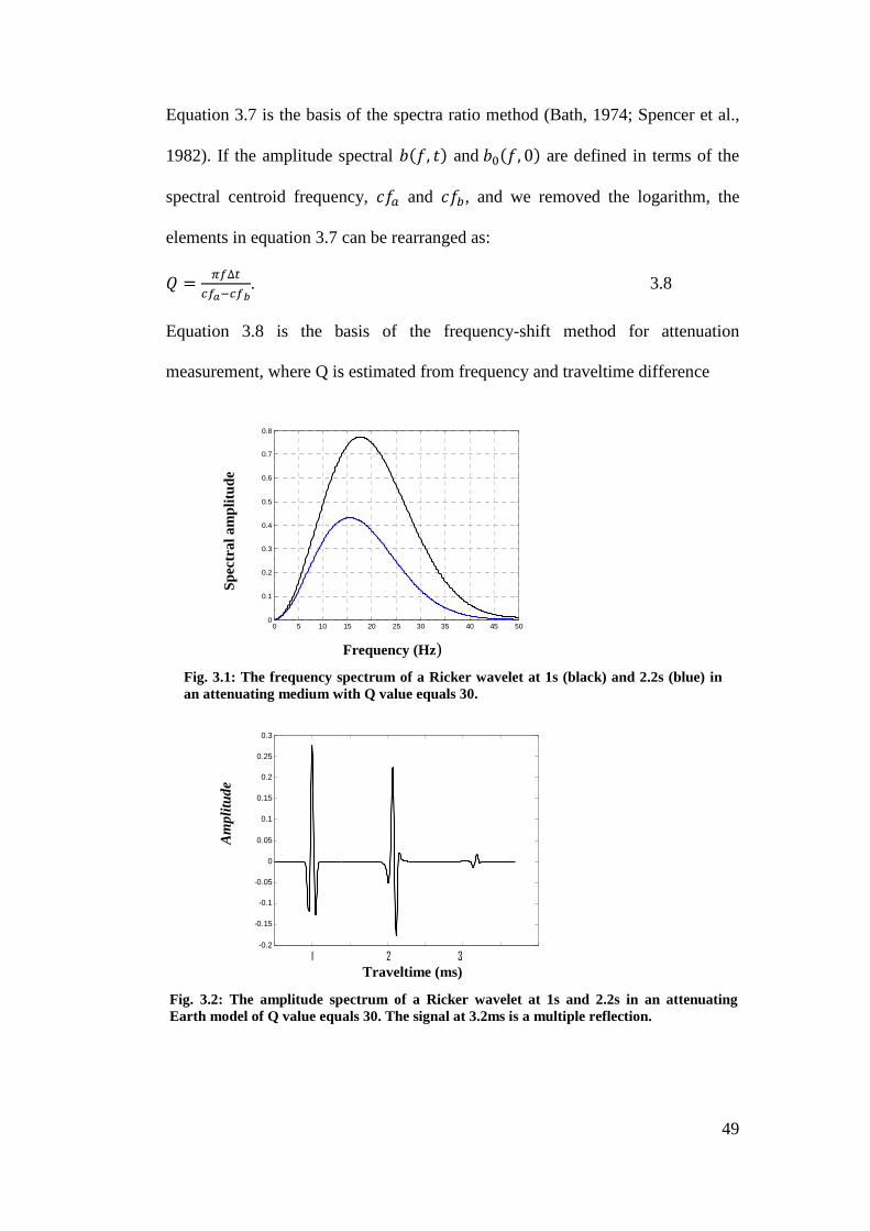
49
Equation 3.7 is the basis of the spectra ratio method (Bath, 1974; Spencer et al.,
1982). If the amplitude spectral %&3, <� and %(&3, 0� are defined in terms of the
spectral centroid frequency, ]3o and ]3G, and we removed the logarithm, the
elements in equation 3.7 can be rearranged as:
� /0∆HN0��N0Æ. 3.8
Equation 3.8 is the basis of the frequency-shift method for attenuation
measurement, where Q is estimated from frequency and traveltime difference
0 1 2 3 4 5 6 7-0.2
-0.15
-0.1
-0.05
0
0.05
0.1
0.15
0.2
0.25
0.3
0 5 10 15 20 25 30 35 40 45 500
0.1
0.2
0.3
0.4
0.5
0.6
0.7
0.8
Fig. 3.1: The frequency spectrum of a Ricker wavelet at 1s (black) and 2.2s (blue) in an attenuating medium with Q value equals 30.
Am
plitu
de
Frequency (Hz)
Spe
ctra
l am
plitu
de
1 2 3 Traveltime (ms)
Fig. 3.2: The amplitude spectrum of a Ricker wavelet at 1s and 2.2s in an attenuating Earth model of Q value equals 30. The signal at 3.2ms is a multiple reflection.

50
(]3o @ ]3G and ∆< ) between the incident and the transmitted signals (see, Quan
and Harris, 1997; Zhang and Ulrych, 2002). ]3 is a spectra parameter known as
the centroid frequency. The centroid frequency is an average spectra parameter
(Barnes, 1993) defined as:
]3o l 0Ço&0�Ç�0|Il Ço&0�Ç�0|I , and 3.9
]3G l 0ÇG&0�Ç�0|Il ÇG&0�Ç�0|I . 3.10
For attenuation measurement in the exploration frequency band, it is common to
use an empirical equation to model attenuation (Gladwin and Stacy, 1974;
Toverud and Ursin, 2005). Based on the physical observations shown in figures
3.1 & 3.2; the definition given equation 3.8; and several synthetic experiments, a
statistics-based empirical model for Q measurement is proposed as:
� H6N0�N0Æ�È�Æ&N0�!N0Æ�. 3.11
Where � is the shape factor, a constant used to obtain the best fit to the data for
the various spectral shapes. As pointed out by equations (12), (13) and (14) of
Quan and Harris (1997), the constant � depends on the actual spectral content of
the wavelet, and � varies with the spectral shapes. ÉoG is the average standard
deviation of the incident and transmitted spectral, and < is the traveltime
different. The average standard deviation, ÉoG is:
ÉoG È�~ÈÆ6 , 3.12
where Éo ©Éo6, and ÉG ©ÉG6.
Éo�6 l&0�N0��\o&0��0l o&0��0 , and ÉG�6 l&0�N0Æ�\G&0��0l G&0��0 . 3.13
For a source-receiver offset ', the traveltime < can be expressed (Sheriff and
Geldart, 1985; Burger et al. 1992) as:
0
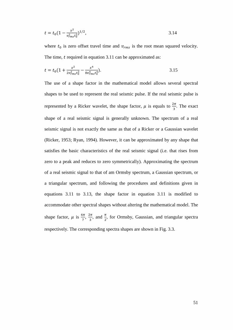
51
< <(&1 @ ,\1_½�\ HI\��/6, 3.14
where <( is zero offset travel time and 2��j is the root mean squared velocity.
The time, < required in equation 3.11 can be approximated as:
< <(&1 P ,\61_½�\ HI\ @ ,�Ê1_½�� HI��. 3.15
The use of a shape factor in the mathematical model allows several spectral
shapes to be used to represent the real seismic pulse. If the real seismic pulse is
represented by a Ricker wavelet, the shape factor, � is equals to 6/� . The exact
shape of a real seismic signal is generally unknown. The spectrum of a real
seismic signal is not exactly the same as that of a Ricker or a Gaussian wavelet
(Ricker, 1953; Ryan, 1994). However, it can be approximated by any shape that
satisfies the basic characteristics of the real seismic signal (i.e. that rises from
zero to a peak and reduces to zero symmetrically). Approximating the spectrum
of a real seismic signal to that of am Ormsby spectrum, a Gaussian spectrum, or
a triangular spectrum, and following the procedures and definitions given in
equations 3.11 to 3.13, the shape factor in equation 3.11 is modified to
accommodate other spectral shapes without altering the mathematical model. The
shape factor, � is Ë/Ì ,
6/� , and /6, for Ormsby, Gaussian, and triangular spectra
respectively. The corresponding spectra shapes are shown in Fig. 3.3.

52
3.4: Synthetic tests and model comparison
Using the Q measurement algorithm described in the section above, seismic
traces are generated in a three-layer attenuating Earth model comprising a shale–
sandstone–shale layered model. The sandstone is partially saturated and has
higher attenuation compared to the underlying and overlying shale layers. The
Earth model and the layer parameters are shown in figure 3.4. The quality factor
in the sandstone layer is represented by Q values of 10, 20, 30, 40, 50, and 100.
Attenuated seismic signals and their multiples are generated from the Earth
model using the algorithm described in Appendix 2A. Q is measured in the
seismic records at the interval that corresponds to the sandstone layer, by
comparing the spectral of the seismic signals that correspond to the top and the
bottom of the sandstone layer. The Q estimates for the various input Q models
are shown in figure 3.5.
Fig. 3.3: The various spectra shapes used in the attenuation model, to represent the real seismic signal. Red is the triangular spectrum, pink is the Ormsby spectrum (or a boxcar), black is the Gaussian spectrum and blue is the Ricker spectrum.
-50 0 500
0.2
0.4
0.6
0.8
1
-50 0 50-0.5
0
0.5
1
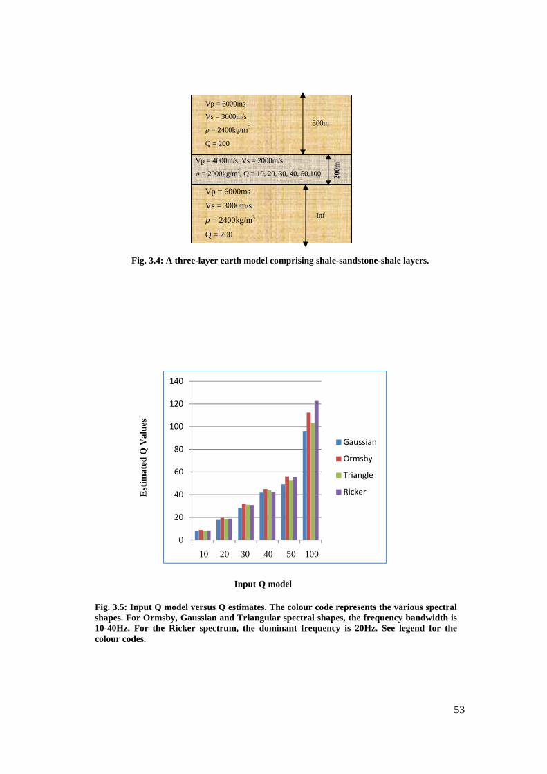
53
Est
imat
ed Q
Val
ues
Fig. 3.4: A three-layer earth model comprising shale-sandstone-shale layers.
Fig. 3.5: Input Q model versus Q estimates. The colour code represents the various spectral shapes. For Ormsby, Gaussian and Triangular spectral shapes, the frequency bandwidth is 10-40Hz. For the Ricker spectrum, the dominant frequency is 20Hz. See legend for the colour codes.
0
20
40
60
80
100
120
140
1 2 3 4 5 6
Gaussian
Ormsby
Triangle
Ricker
Input Q model
10 20 30 40 50 100
200m
Inf
Vp = 6000ms
Vs = 3000m/s x = 2400kg/m3
Q = 200
Vp = 4000m/s, Vs = 2000m/s x = 2900kg/m3, Q = 10, 20, 30, 40, 50,100
300m
Vp = 6000ms
Vs = 3000m/s x = 2400kg/m3
Q = 200
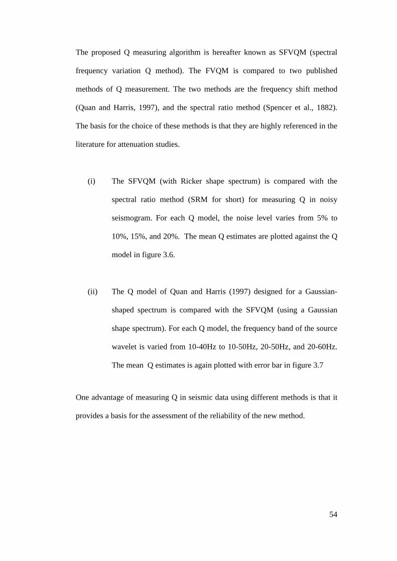
54
The proposed Q measuring algorithm is hereafter known as SFVQM (spectral
frequency variation Q method). The FVQM is compared to two published
methods of Q measurement. The two methods are the frequency shift method
(Quan and Harris, 1997), and the spectral ratio method (Spencer et al., 1882).
The basis for the choice of these methods is that they are highly referenced in the
literature for attenuation studies.
(i) The SFVQM (with Ricker shape spectrum) is compared with the
spectral ratio method (SRM for short) for measuring Q in noisy
seismogram. For each Q model, the noise level varies from 5% to
10%, 15%, and 20%. The mean Q estimates are plotted against the Q
model in figure 3.6.
(ii) The Q model of Quan and Harris (1997) designed for a Gaussian-
shaped spectrum is compared with the SFVQM (using a Gaussian
shape spectrum). For each Q model, the frequency band of the source
wavelet is varied from 10-40Hz to 10-50Hz, 20-50Hz, and 20-60Hz.
The mean Q estimates is again plotted with error bar in figure 3.7
One advantage of measuring Q in seismic data using different methods is that it
provides a basis for the assessment of the reliability of the new method.
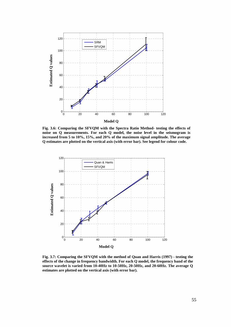
55
Est
imat
ed Q
val
ues
Fig. 3.6: Comparing the SFVQM with the Spectra Ratio Method- testing the effects of noise on Q measurements. For each Q model, the noise level in the seismogram is increased from 5 to 10%, 15%, and 20% of the maximum signal amplitude. The average Q estimates are plotted on the vertical axis (with error bar). See legend for colour code.
0 20 40 60 80 100 1200
20
40
60
80
100
120
SRM
SFVQM
Model Q
Est
imat
ed Q
val
ues
0 20 40 60 80 100 1200
20
40
60
80
100
120
Quan & Harris
SFVQM
Fig. 3.7: Comparing the SFVQM with the method of Quan and Harris (1997) - testing the effects of the change in frequency bandwidth. For each Q model, the frequency band of the source wavelet is varied from 10-40Hz to 10-50Hz, 20-50Hz, and 20-60Hz. The average Q estimates are plotted on the vertical axis (with error bar).
Model Q
56
The results plotted in figure 3.5 show that SFVQM can provide reliable estimates
of Q in synthetic seismograms using any of the spectral shapes. SFVQM is less
sensitive to the interference from noise compared to the spectral ratio method
(figure 3.6). This is because the Q estimates from SFVQM rely on the centroid
frequency – an average spectral parameter, rather than the entire frequency
content of the signal. The error analysis of the Q estimates presented in figure 3.6
shows that the mean error from SFVQM is 9.5%, while the mean error from
SRM is 14.7%. The mean error is estimated as the average of the errors from the
six measurements plotted in figure 3.6. The result plotted in fig 3.7 show that the
SFVQM compares favourably with the method proposed by Quan and Harris
(1997). The mean errors from SFVQM and the method proposed by Quan and
Harris (1997) are 9.8% and 13.4%, respectively. However, it is observed that
SFVQM gives less robust estimates, compared to the other methods, when the
input Q is 100. The synthetic experiment does not consider the tuning effects that
may arise from thin layers. However, it is expected that tuning effects of thin
layers will increase the estimation error in all the methods of Q measurement.
3.5: Q measurement in seismic field data
A set of 3D data from the Gullfaks field is used to test the suitability of the
SFVQM method for Q measurement in field data. The Gullfaks field is located in
the Norwegian sector of the northern North Sea. The data was acquired by
STATOIL in 1985, and donated to Imperial College, London, for PETREL
training. The seismic records represent a traveltime interval of 905 ms, starting
from 1397ms to 2302ms, and cut across two series of sandstones separated by a

57
shale layer. Figure 3.8 shows the survey area. The blue rectangle shows the
position of the analysed traces; the red star shows the position of well A-10; and
the blue vertical line represents the traces along CDP 602 line. The section of the
data selected for Q measurement is informed by the availability of a well in the
area. The well data consist of Time, Porosity, Permeability and Gamma logs
covering a depth range of 1500m to 2416m (see appendix 3A). The information
synthesised from the well logs is used to generate a lithology log and an acoustic
impedance log, to provide guidance in discriminating the reflections that
correspond to lithological boundaries from those that are due to artefacts, noise
and multiples. Based on this approach, the entire time-depth section covered by
the seismic traces is partitioned into four intervals as indicated in the traces
shown figure 3.9. The selected traces were edited to remove traces with
unacceptable level of noise. A total of 500 traces were selected for the Q
measurement. For Q measurement in field data, I assumed that the shape of the
real seismic signal is similar to a Ricker wavelet, and I use the SFVQM with a
Ricker spectrum (i.e. � is 2F 3⁄ ). Seismic signals that correspond to the top and
base of the interval to be analysed for attenuation were isolated using a Hanning
window. To minimise interference from noise, variable window lengths are used
(see also Reine at al., 2009a). The minimum and maximum window lengths used
are 76ms and 98ms, respectively. Fourier transforms are computed within the
window containing each desired event. The spectral parameters required for Q
measurement are computed as defined in equations (3.11) – (3.13).

58
Before the proper Q measurement, the sensitivity of Q estimates to the window
length is tested. Window size is varied within the minimum and maximum (76ms
and 98ms) lengths, and Q measurements are tested using some traces. Results of
the sensitivity test shows that variation in the window length within the
maximum and minimum lengths can influence the Q estimates by 2% to 19%.
Fig. 3.9: Left- some seismic traces within the blue box in figure 3.8. Right- stacked trace along the CDP 602 line. The trace length is subdivided into four intervals; AB, BC, CD and DE. The subdivision is for the purpose of Q measurement only. The 500 traces used for Q measurement are shown in appendix 3A.
Tim
e (m
s)
Fig. 3.8: X and Y Coordinates of the survey area. The blue rectangle shows the position of the traces that were analysed, the red star show the position of the well; and the blue vertical line represents the traces in CDP 602.
Y C
oord
inat
e (m
) x
106
X Coordinate (m) x 105
1400
1500
1600
1700
1800
1900
2000
2100
2200
Tim
e (m
s)
A
B
C
D
E
A
B
C
D
E
Tim
e (m
s)

59
The low error limit is when there is no signal interference (i.e., no noise or
multiple within the window). The error increases when there is spectral
interference (i.e., when noise or multiples is present within the window). For the
real Q analysis, the minimum possible window length is used in order to reduce
signal interference during spectral computation. Whenever possible, the same
window length is used for a signal pair being compared in the measurement.
Important step before computing the spectral parameters is the accurate time
measurement of the reflection events. The definition of arrival time adopted is
the traveltime that corresponds to the maximum amplitude of the desired seismic
event. The time < used for the Q inversion is the difference between traveltime of
paired events – one event corresponding to the top, and the other corresponding
to the bottom of the interval being analysed for attenuation (1/Q). Examples of
the frequency spectral of seismic signals computed at the top and bottom of
interval BC in one of the traces are shown in figure 3.10.
Nor
mal
ised
Spe
ctra
l Am
plitu
de
0 20 40 60 80 100 120
0.05
0.1
0.15
0.2
Frequency (Hz)
Fig. 3.10: The frequency spectrum of the seismic signal corresponding to the top (black) and bottom (blue) of interval BC in one of the traces.

60
-20 0 20 40 60 80 1000
20
40
60
80
100
120
140
160
180
200interval cd
For the purpose of Q estimation, the total travel time represented by the traces is
divided into four intervals: AB, BC, CD and DE, as shown in figure 3.9.
Subsequently, Q is measured in each of the four intervals, trace by trace. The
distribution of Q estimates is shown in figure 3.11.
Distribution of the Q estimates in interval AB. Distribution of the Q estimates in interval BC.
-20 0 20 40 60 80 1000
20
40
60
80
100
120
140
160
180
200
-20 0 20 40 60 80 1000
20
40
60
80
100
120
140
160
180
200
-20 0 20 40 60 80 1000
20
40
60
80
100
120
140
160
180
200
Distribution of the Q estimates in interval CD. Distribution of the Q estimates in interval DE.
Fig. 3.11: Histograms showing the distribution of the Q estimates at the four intervals. The negative values of Q are not considered in the computation of the mean attenuation (1/��).
The inverse Q mean (1/��) is calculated as:
��½ �M ∑ ��²M��� . 3.16

61
Where ��² is the inverse of the individual Q value plotted in figure 3.11. B = 1, 2,
3, 4, 5, . . . . ., 500. The negative values of Q were considered as outliers, and
were excluded from the computation of 1/��. The outliers constitute about 5%
of the total estimates. The 1/�� and the standard deviation, É calculated for each
interval are shown in table 3.1. A MATLAB code written to measure Q in the
field data is shown in appendix 3B. Because MATLAB cannot read seismic data
in SEGY format, a SEISLAB interface on MATLAB is used.
Table 3.1: The mean attenuation (1/��) and the standard deviation (�) calculated for the four intervals.
Interval
(m)
AB
1495-1673
BC
1673-1737
CD
1737-1839
DE
1839-2242
1 ��⁄ 0.0196 0.0573 0.0389 0.0220
É 0.0045 0.0338 0.0180 0.0075
Figure 3.12 shows the attenuation profile representing the 1/�� calculated from
500 traces in the vicinity of the well. The histograms showing the distribution of
the positive 1/Q values are shown in appendix 3C. Following this, the traces
corresponding to CDP 602 are stacked. Attenuation (or 1/Q) is measured in the
stacked traces using the SFVQM and spectral ratio method (SRM). The results of
the measurements are presented in table 3.2. The attenuation profiles plotted
from the 1/Q measured in the stacked trace, using the SFVQM and SRM is
shown figure 3.13. Maps showing Q distribution in the four intervals are shown
in appendix 3D.
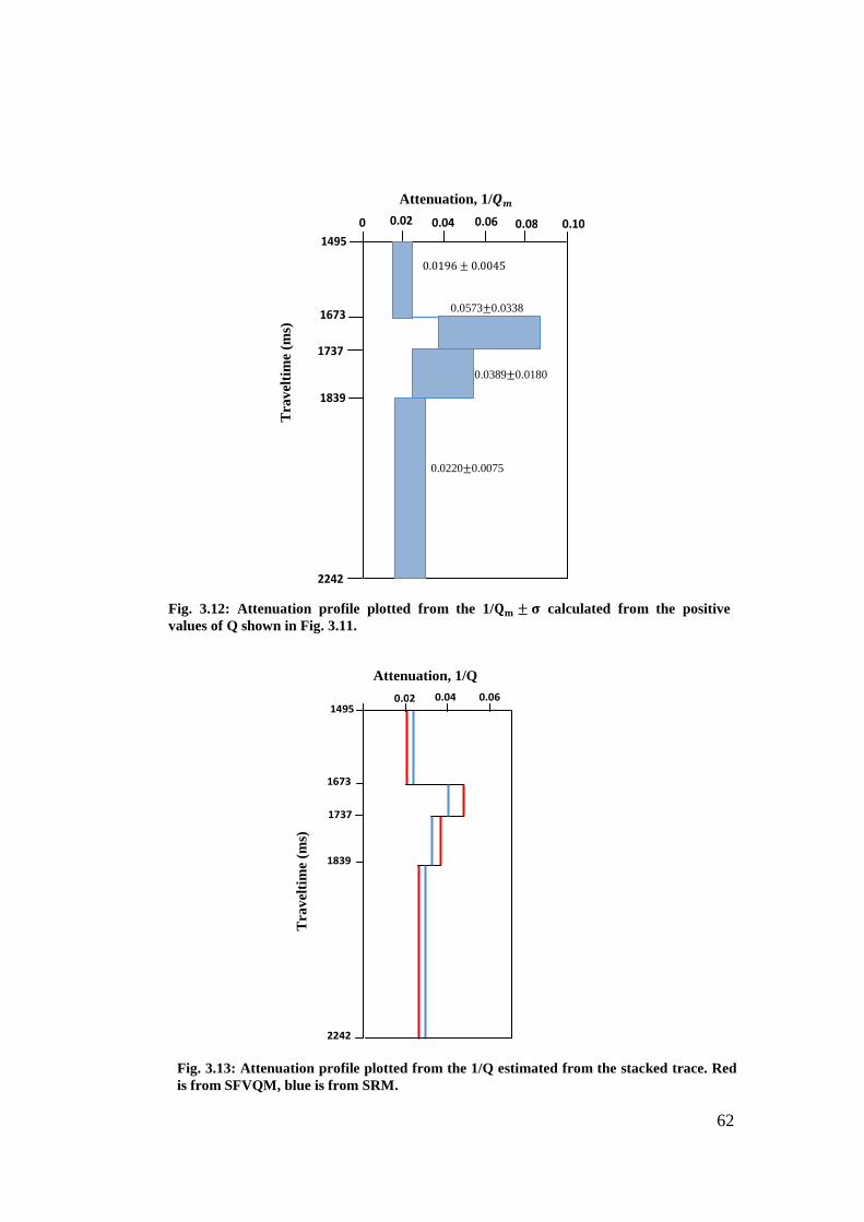
62
1495
2242
1839
1673
1737
0.02 0.06 0.04
Tra
velti
me
(ms)
T
rave
ltim
e (m
s)
Attenuation, 1/Q
Fig. 3.12: Attenuation profile plotted from the 1/�� � calculated from the positive values of Q shown in Fig. 3.11.
Fig. 3.13: Attenuation profile plotted from the 1/Q estimated from the stacked trace. Red is from SFVQM, blue is from SRM.
0.0196 0.0045
0.0573 0.0338
0.0389 0.0180
0.0220 0.0075
0.02 0.06 0.04 0.08 0.10 0
1495
1673
1737
1839
2242
Attenuation, 1/̈ ´
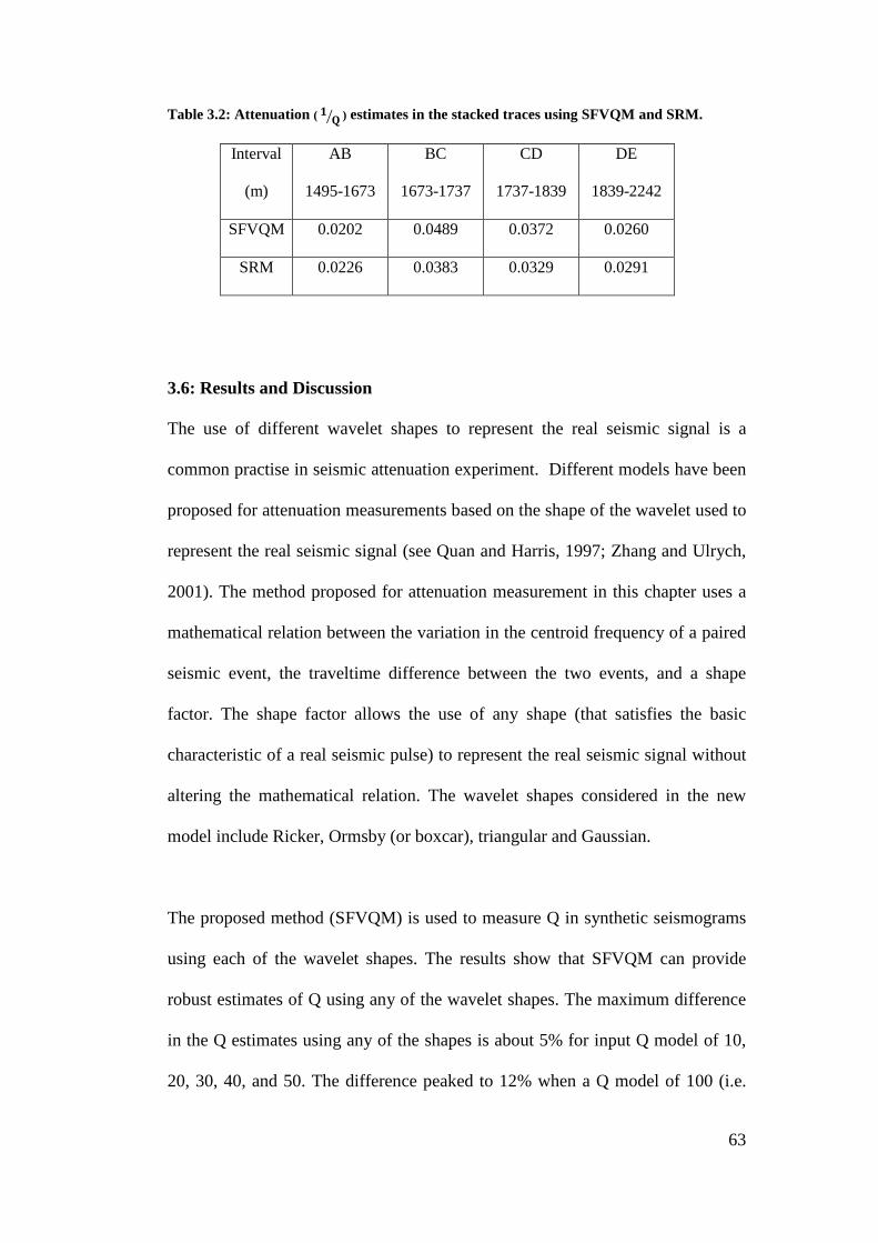
63
Table 3.2: Attenuation ( � � � ) estimates in the stacked traces using SFVQM and SRM.
Interval
(m)
AB
1495-1673
BC
1673-1737
CD
1737-1839
DE
1839-2242
SFVQM 0.0202 0.0489 0.0372 0.0260
SRM 0.0226 0.0383 0.0329 0.0291
3.6: Results and Discussion
The use of different wavelet shapes to represent the real seismic signal is a
common practise in seismic attenuation experiment. Different models have been
proposed for attenuation measurements based on the shape of the wavelet used to
represent the real seismic signal (see Quan and Harris, 1997; Zhang and Ulrych,
2001). The method proposed for attenuation measurement in this chapter uses a
mathematical relation between the variation in the centroid frequency of a paired
seismic event, the traveltime difference between the two events, and a shape
factor. The shape factor allows the use of any shape (that satisfies the basic
characteristic of a real seismic pulse) to represent the real seismic signal without
altering the mathematical relation. The wavelet shapes considered in the new
model include Ricker, Ormsby (or boxcar), triangular and Gaussian.
The proposed method (SFVQM) is used to measure Q in synthetic seismograms
using each of the wavelet shapes. The results show that SFVQM can provide
robust estimates of Q using any of the wavelet shapes. The maximum difference
in the Q estimates using any of the shapes is about 5% for input Q model of 10,
20, 30, 40, and 50. The difference peaked to 12% when a Q model of 100 (i.e.

64
low attenuation) is considered. Compared to the spectral ratio method (SRM),
SFVQM is less sensitive to noise interference. This is because SFVQM relies on
the centroid frequency- an average of the entire frequency content of the signal,
while SRM relies on the entire frequency content in the signal bandwidth. The
error in Q estimates due to the effects of noise interference is 9.5% for the
SFVQM and 13.4% for the SRM. When tested for the effects of the change of
frequency bandwidth, SFVQM shows less sensitivity compared to the method
proposed by Quan and Harris (1997). The errors are 9.8% and 14.7%, for
SFVQM and the method of Quan and Harris (1997), respectively.
Q measurements were performed on 500 traces selected from the seismic data
recorded in the Gullfaks field, North Sea, Norway. The data length is partitioned
into four sections: AB, BC, CD, and DE. The estimated mean attenuation (1/��)
and the standard deviation (É) for these intervals are shown in table 3.1. The
attenuation profile plotted from the 1/Q measured in the CDP-stacked trace
(figure 3.9b left), using the SFVQM and SRM are comparable, and they agree
qualitatively with the attenuation profile plotted from the 1/��. The mean
attenuation 1/�� computed from the 500 measurements and 1/Q measured in the
traces stacked along the CDP 602 line show that interval BC has the highest
attenuation value, and that interval AB has the lowest attenuation value. The
values of 1/�� and 1/Q in measured in interval BC by SFVQM are 0.0573 and
0.0489, respectively. While the 1/�� and 1/Q measured at interval AB are
0.0196 and 0.0202, respectively. Interval BC which recorded the highest
attenuation value approximately coincides with the shale break that separates the
top and base sandstones. The factor responsible for high attenuation in interval
65
BC compared to the overlying and underlying sandstone cannot be ascertained
from this study. However, results from attenuation measurement by Stainsby and
Worthington (1985) in VSP data recorded in a well from North Sea, Norway,
show that shale in the area has a Q value of 25 3 (i.e., 0.0357 º1/Q º 0.0455).
Toverud and Ursin (2005) also show that Q values in sandstone of the North Sea
Norway ranges between 30 and 40 (i.e., 0.0250 º 1/Q º 0.0333). These figures
are in considerable agreement with those recorded by SFVQM.
3.7: Separating scattering attenuation from composite attenuation
Research on seismic attenuation attracted lots of interest in the hydrocarbon
industry because of its potential use for hydrocarbon prospect evaluation. One of
the limitations in the use of attenuation for prospect evaluation is identifying the
portion of the attenuation which is directly related to the internal properties of the
rock. Quantifying the value of the intrinsic attenuation in the composite
attenuation is a key step in the use of attenuation for hydrocarbon exploration
and reservoir characterisation. The attenuation measured in field seismic data is
composite attenuation. It is a combination of the intrinsic and the scattering
attenuation. An approximate value of intrinsic attenuation in the attenuation
measured in seismic field records can be obtained if we have an independent way
of measuring the extrinsic attenuation. In this study, I approximate the scattering
attenuation to the energy loss due to the stratigraphic scattering, as a result of the
changes in the seismic properties of the Earth layers. In stratigraphic scattering,
energy loss is not because it is converted into heat, but, because it is partitioned
and redirected into the unobserved parts of the wavefield (O’Doherty and

66
Anstay, 1971; Cormier, 1989) as the waves travel from one stratigraphic layer to
another. ‘Elastic seismograms’ still carry some hidden but measurable
attenuation due to energy partition, redistribution, and multiple scattering at
lithological interface. To quantify the stratigraphic attenuation, I model and
measure the attenuation that will occur in waves travelling in a layer of interest,
without measuring the attenuation that is due to the intrinsic properties of the
layer. I generated full elastic plane wave seismograms, without considering the
Earth’s Q effects, using information from well log. Then, I measure the
scattering attenuation that will occur (due to reflection, transmission and multiple
scattering) in the layer, by comparing the spectral of the seismic signals that
correspond to the top and bottom of the layer. Using the additive law of
attenuation (Dainty, 1981; Richard and Menke, 1983; Mayeda et al., 1992), the
intrinsic attenuation (1/��MH) is the difference between the composite attenuation
(1/�NO) measured in the field data and the scattering attenuation (1/�jN)
measured in the synthetic equivalence of the field seismograms. The relationship
between the three elements of attenuation is defined in equation 3.1, and restated
in equation 3.16 for ease of reference.
���¹ ���Z P ��¸Ó�. 3.17
The well logs and the seismic data recorded in the Gullfaks field, North Sea
Norway is used to demonstrate the process of quantifying the intrinsic
attenuation. The well logs and the seismic data have been presented in appendix
3A. As the available well log suite does not contain velocity and density data, a
velocity model for the logged depth is calculated using the Gassman (1951)
relation. The bulk density of the rock is estimated using Hilterman (2001)
relation. The density and velocity models are shown in figure 3.14, and the layer
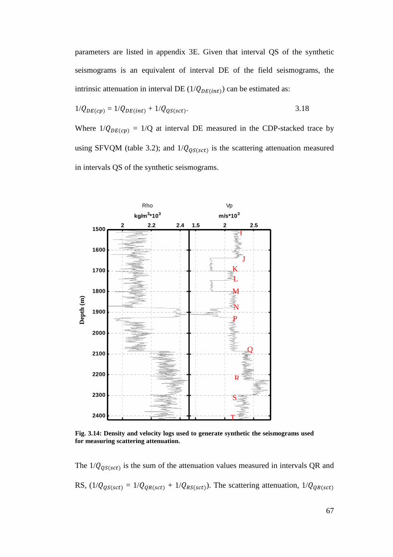
67
parameters are listed in appendix 3E. Given that interval QS of the synthetic
seismograms is an equivalent of interval DE of the field seismograms, the
intrinsic attenuation in interval DE (1/�Ô5&�MH�) can be estimated as:
1/�Ô5&NO� = 1/�Ô5&�MH� + 1/���&jNH�. 3.18
Where 1/�Ô5&NO� = 1/Q at interval DE measured in the CDP-stacked trace by
using SFVQM (table 3.2); and 1/���&jNH� is the scattering attenuation measured
in intervals QS of the synthetic seismograms.
The 1/���&jNH� is the sum of the attenuation values measured in intervals QR and
RS, (1/���&jNH� = 1/���&jNH� + 1/���&jNH�). The scattering attenuation, 1/���&jNH�
1.5 2 2.5
Vp
m/s*103
2 2.2 2.41500
1600
1700
1800
1900
2000
2100
2200
2300
2400
Rho
kg/m3*103
I
J K L
M
N
P
Q
R
S
Fig. 3.14: Density and velocity logs used to generate synthetic the seismograms used for measuring scattering attenuation.
Dep
th (
m)
T

68
and 1/���&jNH� estimated in interval QR and RS are 0.0054 and 0.0068,
respectively. From equation 3.17, the intrinsic attenuation at interval DE
(1/��MHÔ5) is estimated as:
1/��MH� = 0.0260 - (0.0054 + 0.0068) = 0.0138
It is important to mention that the last paragraph of this section is only for the
purpose of demonstration of the procedure for quantifying intrinsic attenuation.
The key point here is not the values of Q obtained but the description of the
process. A comprehensive well log suite containing all the required rock
properties would be more appropriate for the exercise.
3.8: Conclusion
A new method (SFVQM) for measuring Q-factor has been presented in this
chapter. The chapter shows that SFVQM can provide reliable estimates of Q in
synthetic data using any of the spectral shapes commonly assumed for the real
seismic signal. The new method is less sensitive to the interference from noise,
and the change of frequency bandwidth, compared to the SRM and the method
proposed by Quan and Harris (1997). The consistencies in the attenuation
profiles plotted from the 1/�� and 1/Q measured in field seismic data using
SFVQM and the SRM show that SFVQM can provide robust estimates of
attenuation from seismic data. Intrinsic attenuation dominates the extrinsic
attenuation in the composite attenuation measured in the seismic data. Knowing
the value of the intrinsic attenuation in the composite attenuation is a key step in
the use of attenuation for hydrocarbon prospect evaluation. The applications of

69
seismic Q factor are inexhaustible. Its uses include amplitude restoration before
AVO analysis, pre-stack Q-migration and reservoir characterisation.

70
Chapter Four
ROCK PHYSICS DIAGNOSTICS, ATTENUATION MEASUREMENT
AND ANALYSES IN WELLS
71
4.1: Abstract
P-wave and S-wave inverse quality factors (�O�� and �j��) are estimated from the
log data recorded in well A-10 of Gullfaks Field, North Sea, Norway. The results
show that the P-wave inverse quality factor is generally higher in hydrocarbon
saturated rocks than in brine (water) saturated rocks, while the S-wave inverse
quality factor does not show a dependence on fluid content. The range of �¹!"��!"
values measured in gas, water and oil saturated sands are 0.56 – 0.78, 0.39 –
0.55, and 0.35 – 0.41, respectively. A cross plot of the ratio of P-wave to S-wave
inverse quality factors (� !"�#!") with the ratio of P-wave to S-wave velocities (
$ $#)
clearly distinguishes gas sand from water sand and water sand from oil sand. Gas
sand is characterised by the highest � !"�#!" and the lowest
$ $# ratios; oil sand is
characterised by the lowest � !"�#!" and the highest
$ $#; and water sand is
characterized by the $ $# and
� !"�#!" values that plotted between those of the gas and
oil sand. The signatures of the bulk modulus, the Lame’s first parameter, and the
compressional modulus (a hybrid of bulk and shear modulus) show sensitivity to
both the pore fluid and rock mineral matrix. These moduli provide preliminary
identification for sand intervals saturated with different pore fluids.
4.2: Introduction
Attenuation analysis on recorded well logs can provide crucial additional
dimensions to the existing exploration techniques (e.g., Amplitude-versus-Offset,
72
AVO) if realistic rock physics models for the static (porosity, permeability,
mineralogy) and dynamic (saturation, pressure) reservoir properties are available.
Without a good understanding of the geology and the underlying rock physics, it
is impossible to interpret the time variant changes in pore-pressure and saturation
(Andersen et al., 2009). The effect of pore fluid changes on attenuation can be
estimated from rock and fluid properties obtained in recorded well logs and the
mineral composition obtained from geological information, using theoretical
rock physics relations. The change of pore fluid or saturation levels can be
related to the elastic modulus of the rock using the rock physical model of
Gassmann (1951) or Mavko et al. (1995). Therefore, changes in rock modulus
with frequency (modulus-frequency–dispersion) can be linked to the inverse
quality factor (���� via standard linear solid equation, SLS (Mavko et al., 1998).
P- and S-wave attenuation pseudo-logs can be computed from well data as the
difference between high and low frequency moduli using the Kramers-Kronig
relation and the standard linear solid model (Mavko et al., 1998; Dvorkin and
Uden, 2004; Dvorkin and Mavko, 2006). At low frequencies, a pore-scale fluid
distribution is assumed for the rock. The modulus of the rock at low frequency is
estimated as a function of the bulk modulus of the mixture of the pore fluids. The
bulk modulus of the pore fluid mix is the harmonic average of the modulus of the
individual fluids present in the rock. At high frequency, patch-scale fluid
distribution is assumed for the rock. The patches and the region surrounding
them are saturated with different fluid types. The rock modulus at high frequency
is therefore estimated as the harmonic average of the bulk moduli of the patches
and the surrounding region. Attenuation can be estimated in well data using these
73
theories if information regarding porosity, saturation, density, and clay or shale
volume is available from the well log records. The parameters relating to the
fluid and dry rock properties (e.g., bulk modulus of fluid, density of fluid, dry
rock modulus) were obtained from the literature and are specific to the area
under investigation (Klimentos and McCann, 1990; Mavko and Dvorkin, 2005
and Duffaut et al., 2011). Attenuation analysis supported by rock physics models
that are based on valid geological assumptions can serve as a direct hydrocarbon
indicator, and it can potentially guide exploration decisions where common
exploration techniques (e.g., AVO) fail to produce reliable results.
Elastic moduli respond differently to pore fluid and/or rock mineral matrix. The
differential response of these parameters and their hybrids can be used as a
preliminary diagnosis for fluid and lithology to direct further study. The velocity
of seismic waves propagating through a rock can be strongly affected by the
saturation history and fluid distribution in the rock (e.g., Endress and Knight,
1991, 1998; Cadoret, 1993; Mavko and Nolen-Hoeksema, 1994). Bulk modulus
(C), Lame’s first parameter (9), shear modulus (�) (also known as Lame’s second
parameter), and compressional modulus (z) (a hybrid of bulk and shear
parameters) are elastic parameters that can be used to analyse the physical
properties of rocks. Apart from being basic ingredients for attenuation analyses
in well log data, the moduli are on their own sensitive to pore fluid or rock
mineral matrix (lithology), or to both.
Attenuation measurements in recorded well log data using the standard linear
model and the Kramers-Kronig relation have been carried out by Mavko et al.
74
(2005) and Dvorkin and Mavko (2006). The differences between the work
presented in this thesis and those mentioned above are as follows:
• Mavko et al. (2005) and Dvorkin and Mavko (2006) measured
attenuation in well logs recorded in the Gulf of Mexico. The work
presented in this chapter shows how attenuation can be estimated in well
logs with incomplete datasets, and thus engages some quantitative models
to compute the required data;
• This study presents a robust method of combining elastic and anelastic
properties of P- and S-waves to distinguish fluids in rocks;
• The analysis is applied to a dataset from a different geological setting
(Gullfaks field, North Sea, Norway).
This chapter shows how the elastic and inelastic properties of P-wave and S-
wave estimated based on log data recorded in well A-10 of the Gullfaks field,
North Sea, Norway, can be applied to the analysis of the rocks and fluids
penetrated by the well. The chapter applies the sensitivity of some rock-fluid
elastic modulus (Bulk modulus, Shear modulus, Lame’s first parameter and
compressional modulus) to study the lithology and fluids penetrated by the well.
A step by step procedure for estimating P-wave and S-wave inverse quality
factors from well log data using the theory of modulus-frequency-dispersion
(Mavko et al., 1998) is presented. Following this, a robust technique of combined
elastic and inelastic properties of P- and S-wave is used to distinguish gas from
oil and oil from water. The chapter ends with an overview of the discussions and
a conclusion. Throughout this chapter, inverse quality factor is used
interchangeably with attenuation.
75
4.3: Description of some elastic moduli
An elastic modulus is a rock property that describes the tendency of the rock to
be deformed elastically when a force is applied. The force, in the context of this
study is not a mechanical force, it is the force impacted on the rock by the waves
travelling through the rock. The rock is assumed to be homogeneous and
elastically isotropic. The higher the elastic modulus of a rock, the higher the
rock’s resistance to elastic deformation. The three main types of elastic moduli
commonly used by rock physicists are: bulk modulus, shear modulus, and
Lame’s first parameter. The Lame’s first parameter is also known as the
longitudinal modulus. Another type of elastic modulus that is mentioned in this
thesis is the compressional modulus. Compressional modulus is a hybrid of shear
and bulk moduli. The presence of a fluid in rock affects the bulk moduli,
compressional moduli, and Lame’s first parameter of the rock. Therefore, the
three parameters are useful for fluid unit interpretation. These parameters are also
known as P-type parameters (Yuedong and Hongwei, 2007). The shear modulus
of a rock does not depend on the presence of fluid, and thus, it cannot be used for
fluid unit interpretation. The higher the viscosity of the fluid, the higher the P-
type parameters of the rock. All the elastic moduli are measured in Pascal.
Shear modulus, Õ: The shear modulus of a rock describes the resistance of the
rock to deformation, when a force is applied to one of its surfaces while the
opposite surface is experiencing an opposing force. Shear modulus is also known
as the rigidity modulus or the Lame’s second parameter. It is usually explained in
terms of the ratio of shear stress to shear strain. The velocity of a shear wave in a
76
rock is controlled by the shear modulus of the rock. The shear modulus can be
defined in terms of the Young’s Modulus (7) and Poisson’s ratio (2) as:
� 7 2&1 P 2�⁄ , 4.1
or in terms of the shear velocity (Tj) and density (x) as:
� &Tj�6x. 4.2
Bulk modulus (K): the bulk modulus of a rock is a measure of the ability of the
rock to resist change of volume due to the compressional forces acting on all its
surfaces. Bulk modulus is the reciprocal of compressibility. It is also known as
the modulus of volume elasticity, and it is generally defined as the ratio of the
applied pressure to the strain. Bulk modulus can be estimated from shear
modulus and Poisson’s ratio (Wikiversity, 2012) as:
� 2�&1 P 2� 3&1 @ 22�⁄ , 4.3
or from the shear modulus and Lame’s first parameter (Mavko et al., 1998) as:
� 9 P �&2 3⁄ �. 4.4
Compressional modulus (¤): the compressional modulus of a rock describes
the elastic behaviour of the rock when both bulk and shear moduli are acting on
the rock. It is the measure of the rock’s resistance to dynamic compressional
stress. Compressional modulus is also known as P-wave modulus. It can be
define in term of the bulk and shear modulus as:
z � P &4 3�⁄ �, 4.5
or in terms of the bulk modulus and Poisson’s ratio (Wikipedia, 2012) as:
z 3�&1 @ 2� &1 P 2�⁄ . 4.6

77
Lame’s first parameter (Ö�: The Lame’s first parameters is an elastic property
of a rock that describes the resistance of the rock to the compressional
deformation posed by forces acting on the longitudinal axis of the rock. It is also
known as the longitudinal modulus. The Lame’s first parameter can be related to
bulk and shear moduli as:
C 9 P �&2/3�. 4.7
The Lames first parameter can be defined in terms of shear and Poisson’s ratio
as:
9 2�2 &1 @ 22�⁄ . 4.8
The relationships defined in equations 4.2, 4.4, 4.6, and 4.7 are commonly used
by rock physicists to describe shear modulus, bulk modulus, compressional
modulus and Lame’s first parameters, respectively. These equations will be used
in this chapter to estimate the moduli from well log data recorded in the Gullfaks
field.
4.4.1: Rock physics analysis for rock fluid diagnosis
An important goal of petrophysical analyses is to obtain accurate rock physics
parameters to indicate fluid and lithology from borehole (log) data. The three
basic independent elastic parameters that are readily obtained from well logs are
the P-wave velocity (T�), S-wave velocity (T�) and Density (x). These three
fundamental rock properties can be combined to extract rock properties that are
useful to discriminate between lithologies, and can be indicative of the presence
of fluid(s). The elastic properties of rocks can be classified into S-type and P-
type parameters (Yuedong and Hongwei, 2007). S-type parameters are the
parameters that are not sensitive to the presence of fluid (because shear stress
78
cannot transmit in fluids). Examples of S-type parameters include S-wave
velocity, S-wave impedance and shear modulus. Parameters such as P-wave
velocity, P-wave impedance, bulk modulus, Lame’s first parameter, and
compressional modulus are sensitive to fluids. They are generally known as P-
type parameters. Some of the S-type and P-type parameters and their hybrids will
be used for the petrophysical analyses of well data with the goal of delineating
fluid saturated regions, and indicating changes in fluid and lithology.
The log data used for this study is from Well A-10 of the Gullfaks Field, North
Sea Norway. It consists of time, gamma, porosity and permeability data covering
a depth interval from 1500m to 2416m. The well penetrated two sandstone series
separated by a shale section. The log suite used does not contain velocity or
density data that are required for the analysis. However, some quantitative
models (e.g. Timur, 1968, Rider, 1986 and Hilterman, 2001) were used to
compute the well data required for the analysis. Starting from the log data shown
in red in the first four frames of figure 4.1, clay volume (TNÁo�) is predicted from
the Gamma log using Rider (1986) equation:
TNÁo�× ��&1oÁØ8����&��M���&�o,����&ÙÚÛ� . 4.9
Where �Ü&2inÝ)� is the gamma ray value. �Ü&RBQ� and �Ü&Ri'� are the
minimum and maximum gamma ray value, respectively, and TNÁo�× is the linear
clay volume. The linearity in the estimated clay volume is removed as:
TNÁo� $ZÞ��ß��6$ZÞ��ß. 4.10
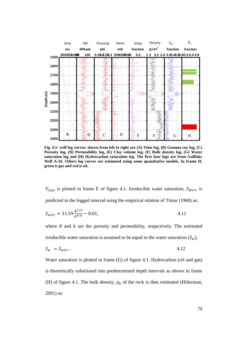
79
TNÁo� is plotted in frame E of figure 4.1. Irreducible water saturation, ��L�� is
predicted in the logged interval using the empirical relation of Timur (1968) as:
�+��� 11.59 y".\à�I.�á @ 0.01, 4.11
where â and C are the porosity and permeability, respectively. The estimated
irreducible water saturation is assumed to be equal to the water saturation (�+),
�+ �+��� . 4.12
Water saturation is plotted in frame (G) of figure 4.1. Hydrocarbon (oil and gas)
is theoretically substituted into predetermined depth intervals as shown in frame
(H) of figure 4.1. The bulk density, xG of the rock is then estimated (Hilterman,
2001) as:
50 100
GR
APIunit
0.150.20.250.3
Porosity
phi
50010001500
Perm
mD
0 0.5 1
Vclay
fraction
2 2.2 2.4
Rho
g/cm3
0.20.40.60.8
SW
fraction
0.2 0.4 0.6
hc
fraction
80090010001500
1600
1700
1800
1900
2000
2100
2200
2300
2400
time
msD
epth
(m)
Fig. 4.1: well log curves: shown from left to right are (A) Time log, (B) Gamma ray log, (C) Porosity log, (D) Permeability log, (E) Clay volume log, (F) Bulk density log, (G) Water saturation log and (H) Hydrocarbon saturation log. The first four logs are from Gullfaks Well A-10. Others log curves are estimated using some quantitative models. In frame H, green is gas and red is oil.
A B C D E F G H
Density
g/cm3
�+ ¾N
80
xG &1 @ y�x�o P y��oH8�x�oH8� P y��ojx�oj P y�£�Áx£�Á, 4.13
where x�o, x�oH8�, x�oj and x£�Á are the density of the grain matrix, water, gas
and oil respectively. ��oH8�, ��oj and �£�Á are the saturations of water, gas and
oil obtained from figure 4.1. Saturation is expressed as a fraction. The density of
the rock matrix is estimated from the clay and quartz composition as:
x�o T�Áo�x�Áo� P &1 @ T�oÁ��x�Øo�Hv, 4.14
where T�Áo�, x�Áo�, x�Øo�Hv are the clay volume, clay density, and quartz
density, respectively. Densities of the rock grains, pore fluids, and bulk moduli of
the fluid, as well as other parameters that are not obtainable from well data (but
usually determined in the laboratory) were obtained from literature published on
the Gullfaks field (Andersen et al. 2009; Duffaut et al. 2011) and Mavko et al.
(1998). These parameters and their values are listed in appendix 4A. The bulk
modulus of the partially saturated rock, �joH in the interval covered by the log
suite is estimated from the Gassmann (1951) formulation as:
�joH �j y�����&�~y������� �#⁄ ~��&��y���~y�#������� �#⁄ . 4.15
The bulk modulus of the saturating fluid �° is estimated as the harmonic average
of the moduli of water, �� and hydrocarbon, �ãN such that:
��� �V�� P ãZ�äZ. 4.16
Where ¾N is the hydrocarbon saturation (plotted in figure 4.1) and can be
substituted with gas or oil saturation. The estimated bulk modulus is plotted with
depth in figures 4.2. The shear modulus, � is estimated using the Pride (2005)
formulation:
� �½�&��y�&��`*y� , 4.17
Where, c �~6*�~* .
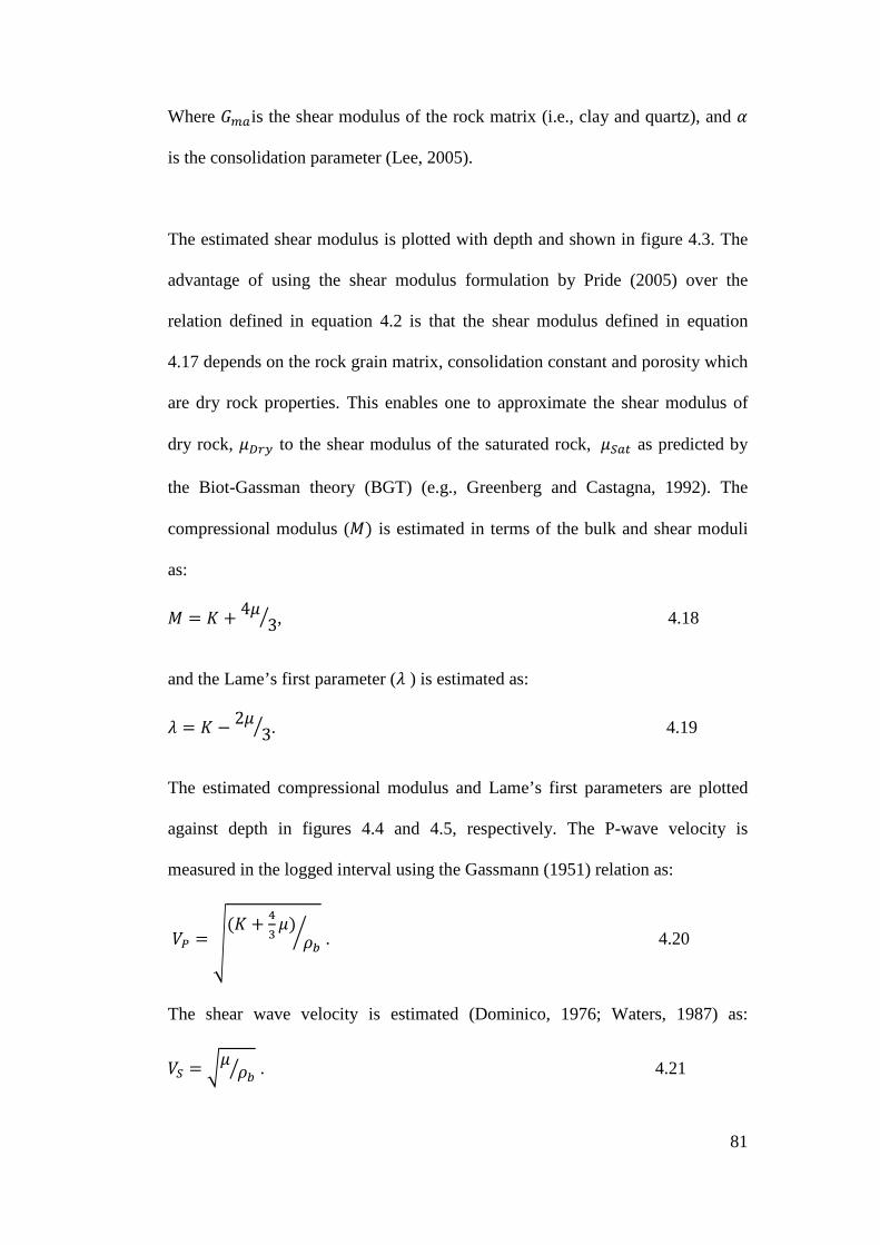
81
Where ��ois the shear modulus of the rock matrix (i.e., clay and quartz), and .
is the consolidation parameter (Lee, 2005).
The estimated shear modulus is plotted with depth and shown in figure 4.3. The
advantage of using the shear modulus formulation by Pride (2005) over the
relation defined in equation 4.2 is that the shear modulus defined in equation
4.17 depends on the rock grain matrix, consolidation constant and porosity which
are dry rock properties. This enables one to approximate the shear modulus of
dry rock, ��� to the shear modulus of the saturated rock, ��oH as predicted by
the Biot-Gassman theory (BGT) (e.g., Greenberg and Castagna, 1992). The
compressional modulus (z� is estimated in terms of the bulk and shear moduli
as:
z � P 4� 3� , 4.18
and the Lame’s first parameter (9 ) is estimated as:
9 � @ 2� 3� . 4.19
The estimated compressional modulus and Lame’s first parameters are plotted
against depth in figures 4.4 and 4.5, respectively. The P-wave velocity is
measured in the logged interval using the Gassmann (1951) relation as:
T� å&� P �� �� xGæ . 4.20
The shear wave velocity is estimated (Dominico, 1976; Waters, 1987) as:
T� �� xG� . 4.21
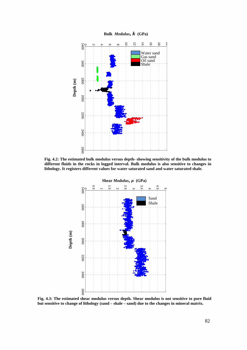
82
14001600
18002000
22002400
26000
0.5 1
1.5 2
2.5 3
3.5 4
4.5 5
Shear Modulus, Õ (GPa)
Dep
th (
m)
14001600
18002000
22002400
26000 2 4 6 8 10 12 14 16 18 20
Bulk Modulus, ç (GPa)
Water sand Gas sand Oil sand Shale
Fig. 4.2: The estimated bulk modulus versus depth- showing sensitivity of the bulk modulus to different fluids in the rocks in logged interval. Bulk modulus is also sensitive to changes in lithology. It registers different values for water saturated sand and water saturated shale.
Dep
th (
m)
Fig. 4.3: The estimated shear modulus versus depth. Shear modulus is not sensitive to pore fluid but sensitive to change of lithology (sand – shale – sand) due to the changes in mineral matrix.
Sand Shale

83
Dep
th (
m)
Fig. 4.4: Estimated compressional modulus versus depth in the logged interval. The plot shows the sensitivity of compressional modulus to different pore fluids and lithology.
Lame’s Parameter Ö (GPa)
Fig. 4.5: Estimated Lame’s first parameter versus depth. The plot shows the sensitivity of Lame’s first parameter to change of pore fluid. Colour index is shown in the legend.
Dep
th (
m)
Compressional Modulus, ¤ (GPa)
Water sand Gas sand Oil sand Shale
Water sand Gas sand Oil sand Shale

84
Where the shear modulus of the rock (�), bulk modulus of the saturated rock
(�) and the bulk density (xG� are from equations (4.17), (4.15) and (4.12)
respectively. The shear modulus of a saturated rock is the same as the shear
modulus of the dry rock (���� �joH). TO and Tj are plotted against depth in
figures 4.6 and 4.7, respectively. The estimated TO/Tj for the logged depth is
plotted in figure 4.8. It is important to note that sands in the interval between
2100 m and 2416 m are more compacted and less porous due to the weight of
overburden material. The sand is probably over-pressured and if compared to the
shallower sand, would exhibit slightly different properties including density and
velocity, even if they contain the same fluid. This probably explains the observed
increase in the values of velocity and elastic moduli in deep sand relative to the
shallow sand.
14001600
18002000
22002400
26000
0.5 1
1.5 2
2.5 3
3.5 4
P-wave velocity èé (km/s)
Dep
th (
m)
Fig. 4.6: The estimated P-wave velocity versus depth in the logged interval. P-wave velocity is sensitive to change of pore fluid and lithology.
Water sand Gas sand Oil sand Shale
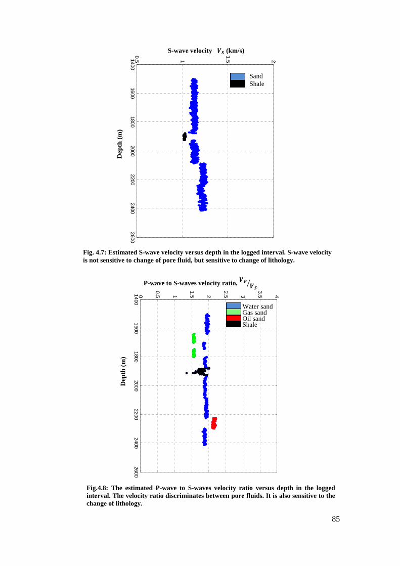
85
14001600
18002000
22002400
26000.5 1
1.5 2
S-wave velocity è« (km/s)
Dep
th (
m)
Fig. 4.7: Estimated S-wave velocity versus depth in the logged interval. S-wave velocity is not sensitive to change of pore fluid, but sensitive to change of lithology.
14001600
18002000
22002400
26000
0.5 1
1.5 2
2.5 3
3.5 4
P-wave to S-waves velocity ratio, èé è«�
Fig.4.8: The estimated P-wave to S-waves velocity ratio versus depth in the logged interval. The velocity ratio discriminates between pore fluids. It is also sensitive to the change of lithology.
Dep
th (
m)
Water sand Gas sand Oil sand Shale
Sand Shale
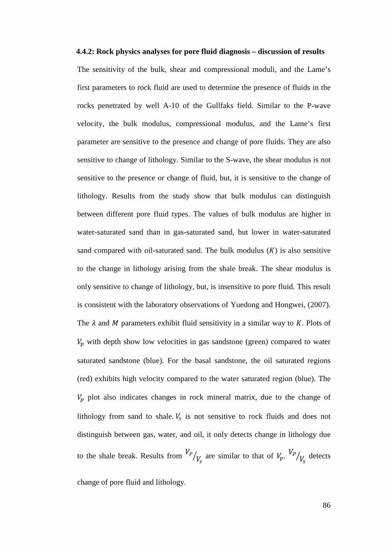
86
4.4.2: Rock physics analyses for pore fluid diagnosis – discussion of results The sensitivity of the bulk, shear and compressional moduli, and the Lame’s
first parameters to rock fluid are used to determine the presence of fluids in the
rocks penetrated by well A-10 of the Gullfaks field. Similar to the P-wave
velocity, the bulk modulus, compressional modulus, and the Lame’s first
parameter are sensitive to the presence and change of pore fluids. They are also
sensitive to change of lithology. Similar to the S-wave, the shear modulus is not
sensitive to the presence or change of fluid, but, it is sensitive to the change of
lithology. Results from the study show that bulk modulus can distinguish
between different pore fluid types. The values of bulk modulus are higher in
water-saturated sand than in gas-saturated sand, but lower in water-saturated
sand compared with oil-saturated sand. The bulk modulus (�) is also sensitive
to the change in lithology arising from the shale break. The shear modulus is
only sensitive to change of lithology, but, is insensitive to pore fluid. This result
is consistent with the laboratory observations of Yuedong and Hongwei, (2007).
The 9 and z parameters exhibit fluid sensitivity in a similar way to �. Plots of
TO with depth show low velocities in gas sandstone (green) compared to water
saturated sandstone (blue). For the basal sandstone, the oil saturated regions
(red) exhibits high velocity compared to the water saturated region (blue). The
TO plot also indicates changes in rock mineral matrix, due to the change of
lithology from sand to shale. Tj is not sensitive to rock fluids and does not
distinguish between gas, water, and oil, it only detects change in lithology due
to the shale break. Results from T� Tj� are similar to that of TO. T� Tj� detects
change of pore fluid and lithology.
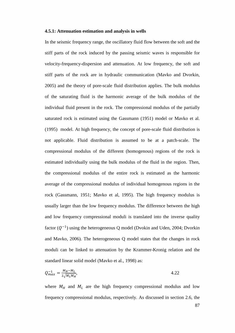
87
4.5.1: Attenuation estimation and analysis in wells
In the seismic frequency range, the oscillatory fluid flow between the soft and the
stiff parts of the rock induced by the passing seismic waves is responsible for
velocity-frequency-dispersion and attenuation. At low frequency, the soft and
stiff parts of the rock are in hydraulic communication (Mavko and Dvorkin,
2005) and the theory of pore-scale fluid distribution applies. The bulk modulus
of the saturating fluid is the harmonic average of the bulk modulus of the
individual fluid present in the rock. The compressional modulus of the partially
saturated rock is estimated using the Gassmann (1951) model or Mavko et al.
(1995) model. At high frequency, the concept of pore-scale fluid distribution is
not applicable. Fluid distribution is assumed to be at a patch-scale. The
compressional modulus of the different (homogenous) regions of the rock is
estimated individually using the bulk modulus of the fluid in the region. Then,
the compressional modulus of the entire rock is estimated as the harmonic
average of the compressional modulus of individual homogenous regions in the
rock (Gassmann, 1951; Mavko et al, 1995). The high frequency modulus is
usually larger than the low frequency modulus. The difference between the high
and low frequency compressional moduli is translated into the inverse quality
factor (���) using the heterogeneous Q model (Dvokin and Uden, 2004; Dvorkin
and Mavko, 2006). The heterogeneous Q model states that the changes in rock
moduli can be linked to attenuation by the Krammer-Kronig relation and the
standard linear solid model (Mavko et al., 1998) as:
��o,�� {ê�{ß6©{ß{ê, 4.22
where zë and z× are the high frequency compressional modulus and low
frequency compressional modulus, respectively. As discussed in section 2.6, the
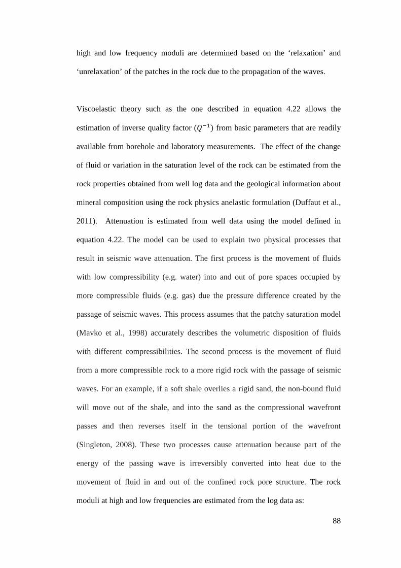
88
high and low frequency moduli are determined based on the ‘relaxation’ and
‘unrelaxation’ of the patches in the rock due to the propagation of the waves.
Viscoelastic theory such as the one described in equation 4.22 allows the
estimation of inverse quality factor (���� from basic parameters that are readily
available from borehole and laboratory measurements. The effect of the change
of fluid or variation in the saturation level of the rock can be estimated from the
rock properties obtained from well log data and the geological information about
mineral composition using the rock physics anelastic formulation (Duffaut et al.,
2011). Attenuation is estimated from well data using the model defined in
equation 4.22. The model can be used to explain two physical processes that
result in seismic wave attenuation. The first process is the movement of fluids
with low compressibility (e.g. water) into and out of pore spaces occupied by
more compressible fluids (e.g. gas) due the pressure difference created by the
passage of seismic waves. This process assumes that the patchy saturation model
(Mavko et al., 1998) accurately describes the volumetric disposition of fluids
with different compressibilities. The second process is the movement of fluid
from a more compressible rock to a more rigid rock with the passage of seismic
waves. For an example, if a soft shale overlies a rigid sand, the non-bound fluid
will move out of the shale, and into the sand as the compressional wavefront
passes and then reverses itself in the tensional portion of the wavefront
(Singleton, 2008). These two processes cause attenuation because part of the
energy of the passing wave is irreversibly converted into heat due to the
movement of fluid in and out of the confined rock pore structure. The rock
moduli at high and low frequencies are estimated from the log data as:
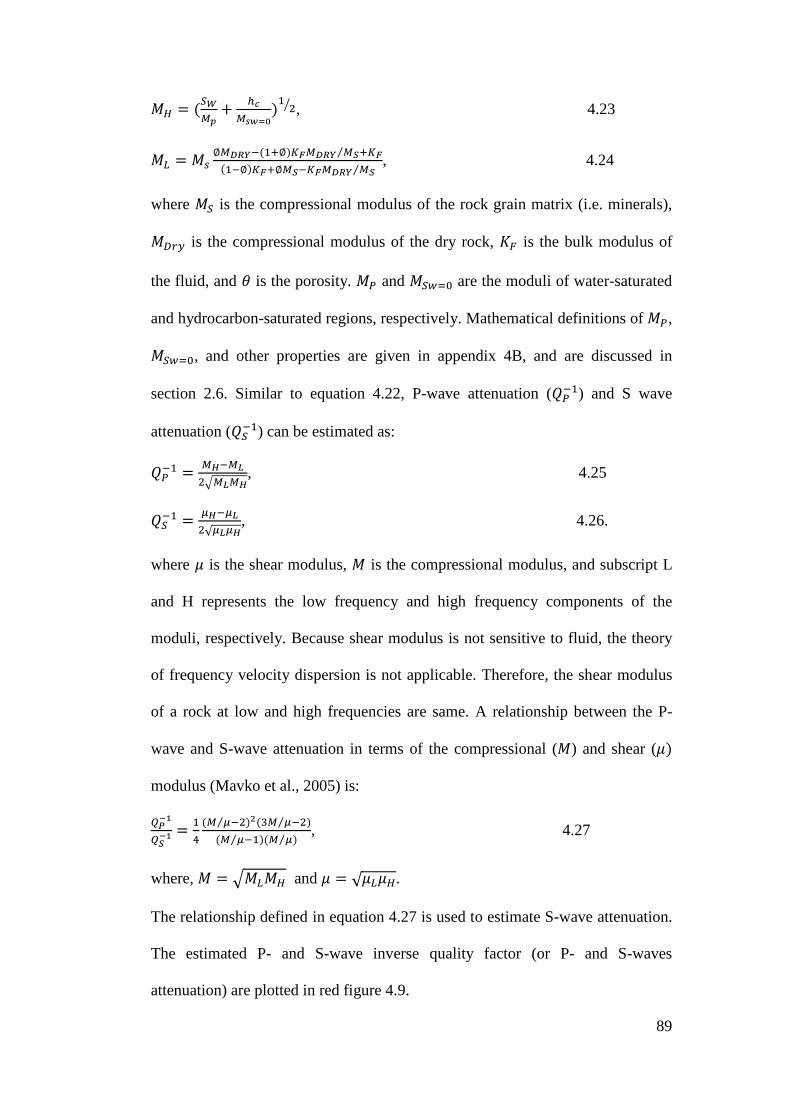
89
zë &��{¹ P ãZ{�V I�� 6� , 4.23
z× zj y{����&�~y���{��� {#⁄ ~��&��y���~y{#���{��� {#⁄ , 4.24
where z� is the compressional modulus of the rock grain matrix (i.e. minerals),
zÔ�� is the compressional modulus of the dry rock, �° is the bulk modulus of
the fluid, and â is the porosity. z� and z�+�( are the moduli of water-saturated
and hydrocarbon-saturated regions, respectively. Mathematical definitions of z�,
z�+�(, and other properties are given in appendix 4B, and are discussed in
section 2.6. Similar to equation 4.22, P-wave attenuation (����) and S wave
attenuation (����) can be estimated as:
���� {ê�{ß6©{ß{ê, 4.25
���� �ê��ß6√�ß�ê, 4.26.
where � is the shear modulus, z is the compressional modulus, and subscript L
and H represents the low frequency and high frequency components of the
moduli, respectively. Because shear modulus is not sensitive to fluid, the theory
of frequency velocity dispersion is not applicable. Therefore, the shear modulus
of a rock at low and high frequencies are same. A relationship between the P-
wave and S-wave attenuation in terms of the compressional (z) and shear (��
modulus (Mavko et al., 2005) is:
� !"�#!" �� &{ ��6�\&�{ ��6�⁄⁄&{ ����&{ ��⁄⁄ , 4.27
where, z ©z×zë and � √�×�ë.
The relationship defined in equation 4.27 is used to estimate S-wave attenuation.
The estimated P- and S-wave inverse quality factor (or P- and S-waves
attenuation) are plotted in red figure 4.9.

90
The results show that the ���� signature is higher in gas saturated sand and oil
saturated sand, than in water saturated sand. On the other hand, ���� does not
differentiate gas sand from water sand, but, it registers higher values in oil sand.
The P- to S-wave inverse quality factor ratio, � !"�#!", is also estimated in the logged
interval and plotted against depth in figure 4.10. A cross plot of velocity ratio, $ $#
and attenuation ratio, � !"�#!" is shown in figure 4.11. The colour codes for the plots
are: blue for water sand, green for gas sand, red for oil sand, and black for shale.
Qualitative interpretation of the results plotted in figure 4.10 shows that: gas sand
exhibits higher � !"�#!" compared to water sand, while oil sand exhibits the lowest
� !"�#!" ratio. In figure 4.11, the three sands plotted at different points on the
attenuation and velocity ratios chart, due to the differences in their pore fluid.
Fig. 4.9: Attenuation log computed from well data with the predicted inverse quality factor (���) in the two last frames. From left to right: porosity, density, water saturation, hydrocarbon saturation (green is gas, red is oil), P-wave inverse quality factor and S-wave inverse quality factor.
2 2.2 2.4
Rho
g/cm3
0.2 0.4 0.6 0.8
SW
fraction
0.2 0.4 0.6
hc
fraction
0.05 0.1 0.15
1/Qp
no
0.2 0.41500
1600
1700
1800
1900
2000
2100
2200
2300
2400
1/Qs
no
Dep
th (m
)
0.150.20.250.31500
1600
1700
1800
1900
2000
2100
2200
2300
2400
Porosity
phiD
epth
(m)
¾N �+ Density g/cm3
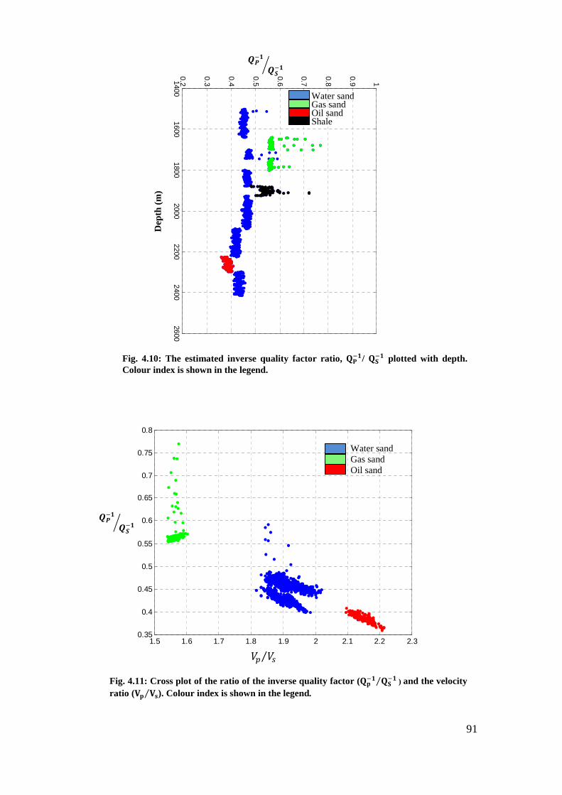
91
14001600
18002000
22002400
26000.2
0.3
0.4
0.5
0.6
0.7
0.8
0.9 1
Dep
th (
m)
¨é�� ¨«��æ
1.5 1.6 1.7 1.8 1.9 2 2.1 2.2 2.30.35
0.4
0.45
0.5
0.55
0.6
0.65
0.7
0.75
0.8
¨é�� ¨«��æ
Water sand Gas sand Oil sand Shale
Water sand Gas sand Oil sand
Fig. 4.10: The estimated inverse quality factor ratio, ����/ ���� plotted with depth. Colour index is shown in the legend.
Fig. 4.11: Cross plot of the ratio of the inverse quality factor (���� ����⁄ ) and the velocity ratio (�� ��⁄ ). Colour index is shown in the legend.
TO Tj⁄
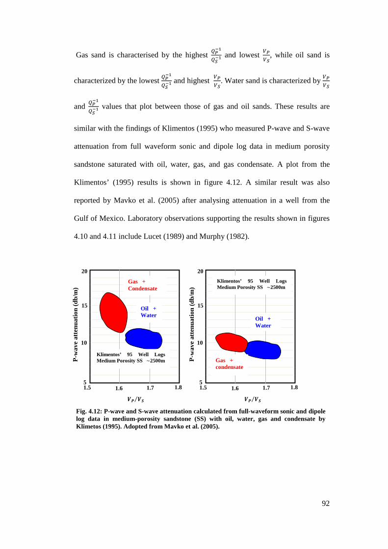
92
Gas sand is characterised by the highest � !"�#!" and lowest
$ $#, while oil sand is
characterized by the lowest � !"�#!" and highest
$ $#. Water sand is characterized by $ $#
and � !"�#!" values that plot between those of gas and oil sands. These results are
similar with the findings of Klimentos (1995) who measured P-wave and S-wave
attenuation from full waveform sonic and dipole log data in medium porosity
sandstone saturated with oil, water, gas, and gas condensate. A plot from the
Klimentos’ (1995) results is shown in figure 4.12. A similar result was also
reported by Mavko et al. (2005) after analysing attenuation in a well from the
Gulf of Mexico. Laboratory observations supporting the results shown in figures
4.10 and 4.11 include Lucet (1989) and Murphy (1982).
èé è«⁄ èé è«⁄
Fig. 4.12: P-wave and S-wave attenuation calculated from full-waveform sonic and dipole log data in medium-porosity sandstone (SS) with oil, water, gas and condensate by Klimetos (1995). Adopted from Mavko et al. (2005).
10
15
20
5 1.5 1.6 1.7 1.8
10
15
20
5 1.5 1.6 1.7 1.8
Klimentos’ 95 Well Logs Medium Porosity SS ~2500m
Gas + Condensate
Oil + Water
Gas + condensate
Klimentos’ 95 Well Logs Medium Porosity SS ~2500m
Oil + Water
P-w
ave
atte
nuat
ion
(db/
m)
P-w
ave
atte
nuat
ion
(db/
m)
93
4.5.2: Attenuation diagnostics and estimation in wells - discussion of results
Anelastic rock attributes computed from well data using rock-fluid physics
formulations show that attenuation is sensitive to the fluid present in the pore
spaces of rocks. P-wave attenuation distinguishes between water (brine) saturated
sand and gas saturated sand. P-wave attenuation is higher in hydrocarbon
saturated intervals (> 0.15 in some places), compared to water saturated regions
where the attenuation value is less than or equal to 0.1. The S-wave attenuation is
sensitive to rock grain matrix but is generally insensitive to the pore fluid.
High attenuation in the shale interval (1874 m – 1933 m) can be attributed to the
effect of lithologic heterogeneity (figure 4.10) since both sand and shale in the
interval between 1800 m and 2000 m have their pore spaces saturated with the
same kind of fluid (water). Stainsby and Worthington (1985) have earlier
reported high attenuation in the North Sea Shale. P-wave inverse quality factor
(����) is higher in gas sand than in water sand. The S-wave inverse quality factor
(����) is high everywhere in the logged interval relative to the P wave inverse
quality factor. ����does not distinguish between water and gas, but it registered
different signatures for sand and shale. Higher value of ����in the oil saturated
sand compared to the gas and water saturated sands is at variance with theoretical
predictions (Klimentos, 1995) which says ���� is ‘indifferent’ to fluid types.
However, It may be speculated that the high signature of ���� in the oil sand is in
response to high pressure and the change in the bulk density of the fluid. A
complete set of unrelated analyses will be required to better interpret the
observed high ���� in the oil sand. Cross plots of P- to S-wave inverse quality
factor, (���� ����⁄ ) and P- to S-wave velocity ratio (T� T�⁄ ) clearly distinguish
94
gas sand from water sand, and water sand from oil sand. Therefore, attenuation
attributes as well as its cross plot with elastic attributes can be used as
hydrocarbon indicator either to compliment other exploration technique or as a
stand-alone method where other methods (e.g., AVO) do not agree with borehole
results.
4.6: Conclusion
A combination of the elastic moduli and the attenuation properties of P- and S-
waves has been used to study the properties of the rocks penetrated by well A-10
of the Gullfaks field, North Sea, Norway. The Lame’s first parameter, the bulk,
shear and compressional moduli are estimated in the logged interval. The Lame’s
first parameter, the bulk, and compressional moduli show comparable results.
They are lower in gas saturated rock compared to water saturated rock, and
higher in oil saturated rock compared to water saturated rock. Therefore, they can
be used to detect changes in pore fluid. The estimated shear modulus does not
show dependence on pore fluid.
P-wave and S-wave attenuation pseudo-logs are computed for the rock interval
penetrated by well A-10, and used to show the sensitivity of P-wave attenuation
to the presence of hydrocarbon. Hydrocarbon saturated zones exhibit higher P-
wave attenuation than water saturated zones. The range of �¹!"��!" values for gas,
water, and oil saturated sands are 0.56 – 0.78, 0.39 – 0.55, and 0.35 – 0.41,
respectively. A cross plot of the ratio of the P- to S-waves inverse quality factor
and the P- to S-wave velocity ratio distinguished gas from water and water from

95
oil. Attenuation analysis in wells can be used to guide exploration, either to
compliment or confirm other methods (e.g., AVO), in order to mitigate risk in a
search for hydrocarbon accumulation.

96
Chapter Five
Enhanced Seismic Q-Compensation
97
5.1: Abstract
The process of compensating for the effects of attenuation on seismic records is
often marred by numerical instability that causes the introduction of artefacts and
the amplification of seismic noise at the expense of the desired seismic signals.
This often leads to poor seismic image resolution, especially in seismic traces
representing deep-seated high-attenuating rock layers that are typical for
hydrocarbon reservoirs. In an effort to compensate for the effects of attenuation
in seismic records, I propose a frame-work for correcting amplitude diminution
and phase distortion in seismic waves, using a recursive Q inverse filtering
scheme. The time varying inverse Q filter has a Fourier integral representation in
which the direction of propagation for the up-going and down-going waves is
reversed, and the wavenumber is defined as a complex conjugate of the wave
number in the forward propagating waves. To overcome the issue of instability,
the wave number is replaced with slowness to limit the frequency dependence of
the computation, and the Q-compensation algorithm is implemented in a layer-
by-layer step wise approach. The compensation algorithm is tested with synthetic
records and a set of data recorded in the Gullfaks field, North Sea Norway.
Results show that the algorithm is suitable for correcting energy dissipation and
phase dispersion that usually degrade the resolution of subsurface seismic
images. The compensated traces give higher resolved images of the reflectors at
accurate depth location.
98
5.2: Introduction
The amplitude and waveform of seismic waves are strongly impacted by the
anelasticity and inhomogeneity in the media through which the waves travel.
This usually results in loss, in parts, of the desired information in recorded
seismic traces. The loss is often expressed in the form of amplitude diminution,
wavelet distortion and delayed signal arrivals, which in turn degrade the quality
of seismic data. Attenuation causes poor seismic interpretability and contributes
to seismic-well data mis-tie. Correcting for the effects of amplitude reduction and
waveform distortion in recorded seismic traces is beneficial to exploration
seismology for many reasons. One reason is that signal amplitude contains
information about the lithology and reservoir conditions (Winkler and Nur, 1979;
Klimentos and McCann, 1990; Batzle et al, 1996). Another reason is that the
signal arrival time contains information on the location of the reflector. In order
to enhance the interpretability of seismic records, seismic data processing usually
involve a stage where the effects of attenuation on seismic records are corrected.
This step is here known as Q-compensation. Q-compensation is the process by
which the undesirable effects of Earth’s anelasticity and inhomogeneity on
seismic waves (i.e., amplitude attenuation, waveform distortion and velocity
dispersion) are corrected or compensated for.
A common approach to Q-compensation is inverse Q-filtering. Previous work on
the application of inverse Q filtering to the improvement of subsurface seismic
images includes Hale (1981; 1982) , Bickel and Natarajan (1985), Hargreaves
(1991), Mittet et al. (1995), Wang (2002; 2006), Knut-Sorsdal (2009) and Raji
and Rietbrock, (2011). In most of the these studies, the procedure for
99
implementing inverse Q filtering in a stack of layers is not emphasised. Inverse Q
filtering is only discussed for a single layer model. The few algorithms that
considered inverse Q filtering in stack of Earth layers are designed for constant Q
layers (i.e. all the layers are having the same Q value or the same degree of
absorption). In reality, different rock layers usually have different attenuation
characteristics, and different Q values. Apart from this, Q-compensation
algorithms at present have two main limitations: (i) accuracy of the compensated
signal, (ii) and numerical instability. The accuracy of the compensated seismic
signal is a measure of how close the Q-compensated seismic image compares to
the real image of the reflector, if the Earth media were perfectly elastic.
Instability is a common problem of the inverse Q filtering process. It is usually
due to overflow or numerical instability in the estimation of the exponential
functions, especially at high travel time components of the inverse Q-filtered
traces. This problem often leads to the introduction of artefact and the
amplification of ambient noise, in the later part of the seismic traces after Q-
compensation (see figure 5.1).
In order to solve the issue of instability, either an approximation is defined for
the amplitude compensation operator (Wang, 2002; Li et al, 2009) or a
stabilization factor is applied to the amplitude compensation operator (Wang,
2006). A Q-compensation algorithm that uses an amplitude approximation
operator or an amplitude gain limit operator can solve the problem of instability
but cannot recover an absorbed seismic signal whose amplitude is below a set
limit. In other words, such an algorithm cannot recover the highly absorbed
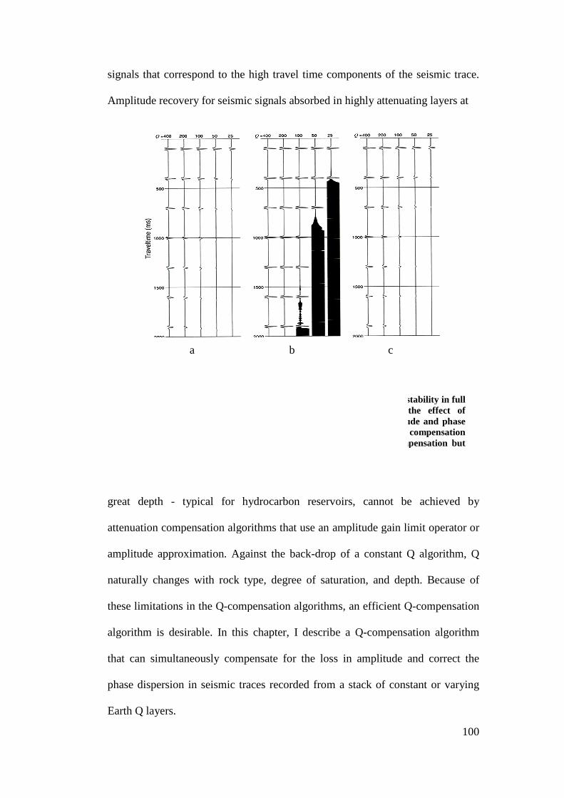
signals that correspond to the high travel time components of the seismic trace.
Amplitude recovery for seismic signals absorbed in highly attenuating layers at
great depth - typical for hydrocarbon reservoirs, cannot be achieved by
attenuation compensation algorithms that use an amplitude gain limit operator or
amplitude approximation. Against the back
naturally changes with rock type,
these limitations in the Q
algorithm is desirable. In this chapter, I describe a Q
that can simultaneously compensate for the loss in amplitude and correct the
phase dispersion in seismic traces recorded fro
Earth Q layers.
a
Figure 5.1: Attenuation and Qamplitude and phase compensation. (a) Synthetic traces showing thattenuation- Q=400, 200, 100, 50, 25 (b) Qcompensation, result which clearly indicates numerical instability. (c) Q compensation for both amplitude and phase compensationband limited amplitude compensation. Adapte
signals that correspond to the high travel time components of the seismic trace.
Amplitude recovery for seismic signals absorbed in highly attenuating layers at
typical for hydrocarbon reservoirs, cannot be achieved by
ation compensation algorithms that use an amplitude gain limit operator or
amplitude approximation. Against the back-drop of a constant Q algorithm, Q
ally changes with rock type, degree of saturation, and depth.
these limitations in the Q-compensation algorithms, an efficient Q
algorithm is desirable. In this chapter, I describe a Q-compensation algorithm
that can simultaneously compensate for the loss in amplitude and correct the
phase dispersion in seismic traces recorded from a stack of constant or varying
b c
Figure 5.1: Attenuation and Q-Compensation – showing the problem of instability in full amplitude and phase compensation. (a) Synthetic traces showing th
Q=400, 200, 100, 50, 25 (b) Q-compensation for full amplitude and phase compensation, result which clearly indicates numerical instability. (c) Q compensation for both amplitude and phase compensation- with full band phase compensaband limited amplitude compensation. Adapted from Wang (2002).
100
signals that correspond to the high travel time components of the seismic trace.
Amplitude recovery for seismic signals absorbed in highly attenuating layers at
typical for hydrocarbon reservoirs, cannot be achieved by
ation compensation algorithms that use an amplitude gain limit operator or
drop of a constant Q algorithm, Q
degree of saturation, and depth. Because of
compensation algorithms, an efficient Q-compensation
compensation algorithm
that can simultaneously compensate for the loss in amplitude and correct the
m a stack of constant or varying
showing the problem of instability in full amplitude and phase compensation. (a) Synthetic traces showing the effect of
compensation for full amplitude and phase compensation, result which clearly indicates numerical instability. (c) Q compensation
with full band phase compensation but

101
In the next sections, I describe the mathematical algorithm and the procedure for
implementing attenuation compensation in seismic traces recorded from various
Earth Q models. To give a clear description of the procedure of Q-compensation,
a brief description of the process of seismic attenuation is given. The Q-
compensation algorithm is tested with synthetic seismograms and a set of data
from the Gullfaks field, North Sea Norway. In order to demonstrate the
improvements in the compensated traces, the difference plots between the
compensated and elastic traces are shown. Following this, the effects of using
incorrect Q for attenuation compensation is examined. The term Q-compensation
is used interchangeably with attenuation compensation throughout this chapter.
5.3: The Q-compensation procedure
Q-compensation is the inverse procedure for seismic attenuation in which wave
propagation is reversed in time along the same path of the forward propagation.
This can be achieved by means of an inverse Q-filter. An important step before
constructing an inverse Q filter is to determine the Q-factor that caused the
attenuation. For the purpose of the Q-compensation algorithm, I briefly review
plane wave propagation in an absorptive Earth medium and then describe the
compensation (inversion) procedure. The plane wave two-way forward
propagation í&C,, h, -� from a source at depth h, to a reflector at further depth
step ∆h and back to a recorder at h (figure 5.2) can be defined as:
í&C,, h P ∆h, -� í&C,, h, -�)'À& î&C @ C,�∆h�. 5.1

102
Where î is the imaginary number and C is the wave-number. C, and - are the
horizontal wave-number and the angular frequency respectively.
C +1&+�, and 5.2
C, +j�M&ï�1&+� .
Where â is the angle of incidence. Following Futterman (1962), I define the
velocity 2&-� of an Earth layer as a frequency dependent complex velocity:
2&-� ð&-� @ ñ6ò&+��, and 5.3
ð&-� 2&1 @ &F���� ln J ++ZK�.
Where ð is the real valued part of the velocity, and ñ6ò&+�� is the imaginary part
of the velocity. � is the quality factor and -N is the reference angular frequency.
Substituting equation (5.3) into equation (5.2), C can be redefined as:
C +ò&+� &1 @ ñ6��. 5.4
For a case of normal incidence, where C, 0. the downward propagation of the
plane wave (i.e. from the source to the reflector) defined in equation 5.1 can be re
written as:
í&h P ∆h, -� í&h, -�exp &@î +ò&+� ∆h�exp &@ +6ò&+�� ∆h�. 5.5
Fig. 5.2: Schematic diagram of wave propagation in an Earth medium. The signal will be compensated for earth Q-effects on its ways from the source (S) down to the reflector and to the receiver (R).
â â x
∆h
z R S
x6, 26, C6
x�, 2�, C�
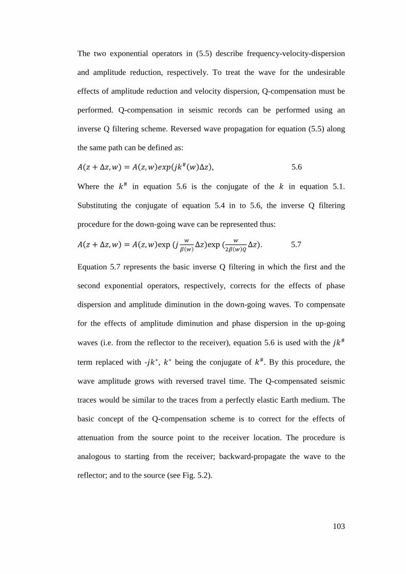
103
The two exponential operators in (5.5) describe frequency-velocity-dispersion
and amplitude reduction, respectively. To treat the wave for the undesirable
effects of amplitude reduction and velocity dispersion, Q-compensation must be
performed. Q-compensation in seismic records can be performed using an
inverse Q filtering scheme. Reversed wave propagation for equation (5.5) along
the same path can be defined as:
í&h P ∆h, -� í&h, -�)'À&îC#&-�∆h�, 5.6
Where the C# in equation 5.6 is the conjugate of the C in equation 5.1.
Substituting the conjugate of equation 5.4 in to 5.6, the inverse Q filtering
procedure for the down-going wave can be represented thus:
í&h P ∆h, -� í&h, -�exp &î +ò&+� ∆h�exp & +6ò&+�� ∆h�. 5.7
Equation 5.7 represents the basic inverse Q filtering in which the first and the
second exponential operators, respectively, corrects for the effects of phase
dispersion and amplitude diminution in the down-going waves. To compensate
for the effects of amplitude diminution and phase dispersion in the up-going
waves (i.e. from the reflector to the receiver), equation 5.6 is used with the îC#
term replaced with -îCô, Cô being the conjugate of C#. By this procedure, the
wave amplitude grows with reversed travel time. The Q-compensated seismic
traces would be similar to the traces from a perfectly elastic Earth medium. The
basic concept of the Q-compensation scheme is to correct for the effects of
attenuation from the source point to the receiver location. The procedure is
analogous to starting from the receiver; backward-propagate the wave to the
reflector; and to the source (see Fig. 5.2).
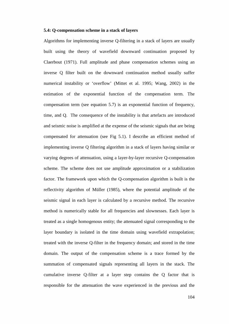
104
5.4: Q-compensation scheme in a stack of layers
Algorithms for implementing inverse Q-filtering in a stack of layers are usually
built using the theory of wavefield downward continuation proposed by
Claerbout (1971). Full amplitude and phase compensation schemes using an
inverse Q filter built on the downward continuation method usually suffer
numerical instability or ‘overflow’ (Mittet et al. 1995; Wang, 2002) in the
estimation of the exponential function of the compensation term. The
compensation term (see equation 5.7) is an exponential function of frequency,
time, and Q. The consequence of the instability is that artefacts are introduced
and seismic noise is amplified at the expense of the seismic signals that are being
compensated for attenuation (see Fig 5.1). I describe an efficient method of
implementing inverse Q filtering algorithm in a stack of layers having similar or
varying degrees of attenuation, using a layer-by-layer recursive Q-compensation
scheme. The scheme does not use amplitude approximation or a stabilization
factor. The framework upon which the Q-compensation algorithm is built is the
reflectivity algorithm of Müller (1985), where the potential amplitude of the
seismic signal in each layer is calculated by a recursive method. The recursive
method is numerically stable for all frequencies and slownesses. Each layer is
treated as a single homogenous entity; the attenuated signal corresponding to the
layer boundary is isolated in the time domain using wavefield extrapolation;
treated with the inverse Q-filter in the frequency domain; and stored in the time
domain. The output of the compensation scheme is a trace formed by the
summation of compensated signals representing all layers in the stack. The
cumulative inverse Q-filter at a layer step contains the Q factor that is
responsible for the attenuation the wave experienced in the previous and the
105
current layer. Given the diagram shown in Fig.5.3, the compensated signal í�
from reflector 3 is:
í� 7�í67�. 5.8
í6 76í�76; í� 7�í(7�; and í( 7(õ(7(. 5.9
Where í6 and í� are the matrices containing the compensated signals from
reflectors 2 and 1, respectively. õ( is the matrix containing the potential
amplitude of the attenuated signal at the base of layer 0. 7� is the phase matrix,
7� ö) ñ�÷�² 00 ) ñ�÷÷�²ø. B is the layer number (B = 0, 1, 2, .... n). In each case, 7� is
an exponential function containing the compensation operators, the thickness,
and velocity of each layer. The terms î, Cù, Cùù and m� represent the imaginary
number, P-wave-number, S-wave-number and the thickness of layer B, respectively. Cù and Cùù contain the Q-factor for correcting amplitude reduction
and phase dispersion (see equation 5.4) experienced by the waves in layer B. The
isolated attenuated event at every layer step is treated with the corresponding
inverse Q-filter in the Fourier domain, and stored in the time domain. To
circumvent numerical instability that often mars the result of inverse Q-filtering:
(i) wave-numbers are replaced with slownesses:
Ý �ú+ ûÚÛ &ï�1&+� , and (horizontal slowness) 5.10a
i �+ &Ý&-��6 @ Ý6�"\, (vertical slowness) 5.10b
where C, and C are defined in equation 5.2; (ii) Q-compensation is implemented
layer by layer in a recursive manner; (iii) and the compensation scheme avoids
working with exponential functions as much as possible - in the algorithm,
exponential function only appears in the phase matrix.
106
The compensated plane wave at a layer step 3 can be defined as:
í�At�, -D í6At6, -D exp Jî +∆s�ò�&+�K exp J +∆s�6ò�&+���K, 5.11
where t is the traveltime, and ∆t� t� @ t6.
The time-domain seismic signal at layer step 3 can be given as:
i�&t�� �6/ l í�&t� , -�m-. 5.12
Similar to Wang (2002), Montana and Margrave (2005) and Knut-Sorsdal
(2009), the complete seismic record across the stack of layers is the summation
of the Q-compensated seismic events (in the time domain) representing the
individual layer in the stack. Each Q-compensated seismic event is the plane
wave reflection at each layer boundary. One advantage of the algorithm is that it
can be used for attenuation compensation in multi-component seismic data when
í� B¢: í� Jüü �üü� �� K. 5.13
Where ü and � represent P-wave and S-wave, respectively. In the reflectivity
matrix, í�, the first letter denotes the incident wave, and the second letter denotes
the secondary wave. Another advantage of the method is that it is built on a
recursive algorithm which is unconditionally stable at all frequencies and
slownesses (see Müller, 1985). “Some algorithms (e.g., see, Kennett 1983,
0 1
2
Q
í(&t(, -� í�&t�, -� í6&t6, -�
íM&tM, -�
Fig. 5.3: A schematic diagram of a stack of homogeneous absorbing layers between two half spaces.
3 í�&t�, -�
Upper half space
Lower half space
107
Sec.6.2.2) suffer from overflow problem in the calculation of exponential
functions for high frequency and slownesses’’ Müller (1985).
5.5: Application to synthetic and field seismic data
The Q-compensation algorithm is tested on synthetic seismic data from a stack of
horizontal homogenous absorbing Earth layers. The Earth models consist of eight
layers whose properties are listed in appendix 5. The layer properties are selected
such that seismic events representing the top layer are separated in time by
300ms from the event representing the next lower layer (see the reference plot in
figures 5.4c & 5.5c). The reference figure is a seismic trace from perfectly elastic
layers, with no attenuation and dispersion. Figure 5.4a shows seismic records
from constant Q layers before attenuation compensation, while figure 5.4b shows
the traces after attenuation compensation. The difference plot between the
reference trace and the Q-compensated traces are shown in figure 5.4d & e.
Figure 5.5a shows synthetic seismic records from a stack of layer having various
degrees of attenuation. Figures 5.5b and c show the seismic records after Q-
compensation and the reference plot, respectively. The difference plot between
the reference and the compensated traces are shown in figure 5.5d & e. Overall,
the Q-compensation algorithm efficiently corrects the phase dispersion and
amplitude diminution. It returns the seismic events to their correct positions with
high resolution. The compensated traces compare favourably with the reference
plot - as if the Earth layers are perfectly elastic. The Q-compensation process
improved the interpretability of the seismic traces compared to the original
(attenuated) traces.
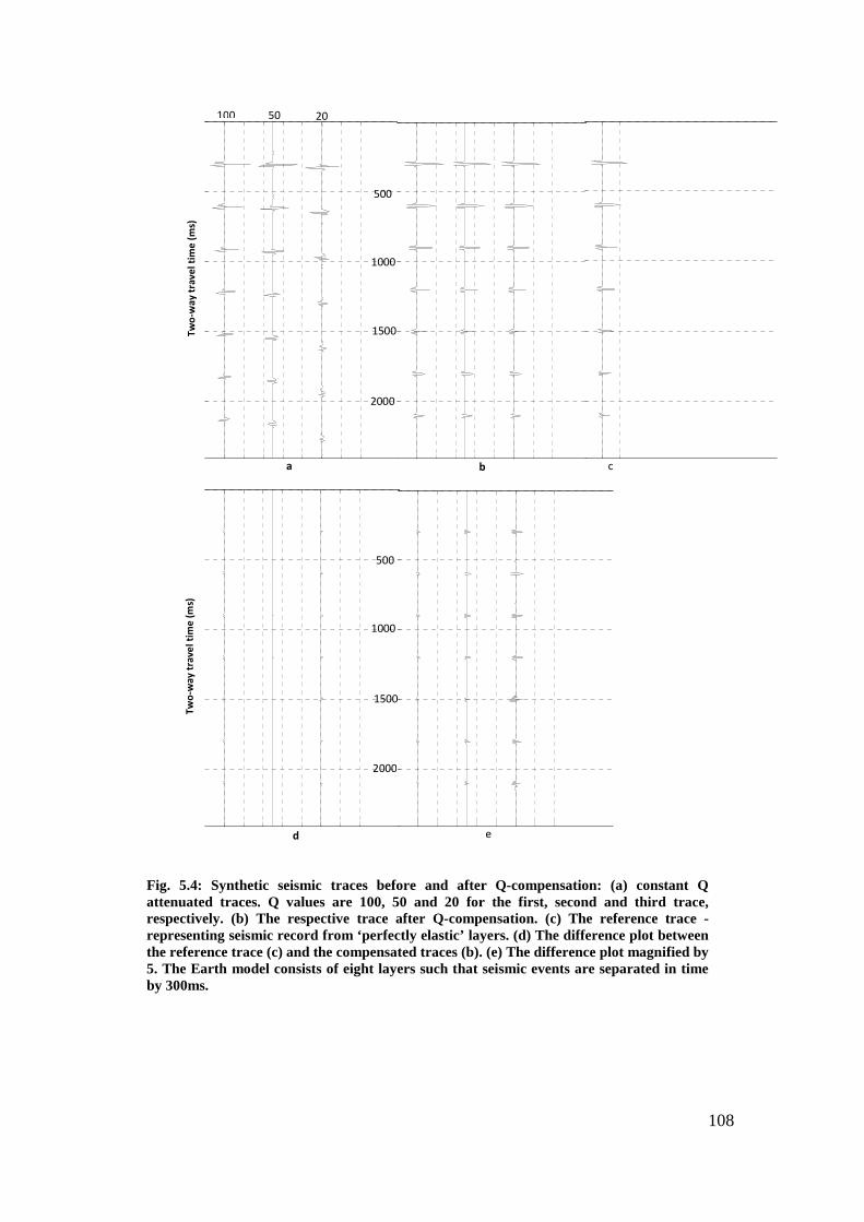
108
500
1000
1500
2000
500
1000
1500
2000
a b c
d e
100 50 20
Tw
o-w
ay
tra
ve
l ti
me
(m
s)
Tw
o-w
ay
tra
ve
l ti
me
(m
s)
Fig. 5.4: Synthetic seismic traces before and after Q-compensation: (a) constant Q attenuated traces. Q values are 100, 50 and 20 for the first, second and third trace, respectively. (b) The respective trace after Q-compensation. (c) The reference trace -representing seismic record from ‘perfectly elastic’ layers. (d) The difference plot between the reference trace (c) and the compensated traces (b). (e) The difference plot magnified by 5. The Earth model consists of eight layers such that seismic events are separated in time by 300ms.
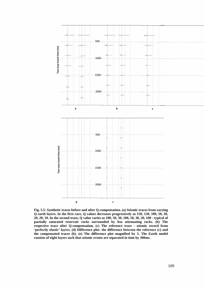
109
500
1000
1500
2000
500
1000
1500
2000
a b c
d e
Tw
o-w
ay
tra
ve
l ti
me
(m
s)
Tw
o-w
ay
tra
ve
l ti
me
(m
s)
Fig. 5.5: Synthetic traces before and after Q-compensation. (a) Seismic traces from varying Q earth layers. In the first race, Q values decreases progressively as 150, 120, 100, 50, 30, 20, 20, 10. In the second trace, Q value varies as 100, 50, 30, 100, 50, 30, 20, 100 - typical of partially saturated reservoir rocks surrounded by less attenuating rocks. (b) The respective trace after Q-compensation. (c) The reference trace - seismic record from ‘perfectly elastic’ layers. (d) Difference plot- the difference between the reference (c) and the compensated traces (b). (e) The difference plot magnified by 5. The Earth model consists of eight layers such that seismic events are separated in time by 300ms.
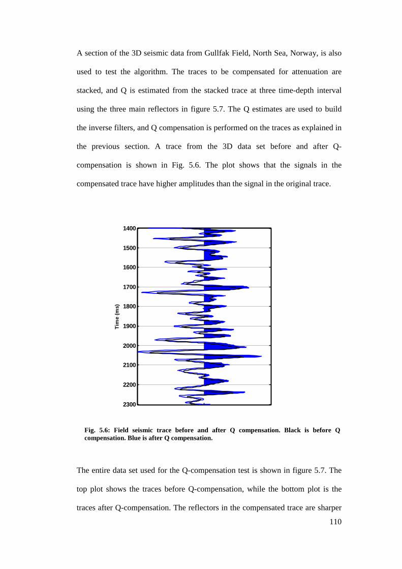
110
A section of the 3D seismic data from Gullfak Field, North Sea, Norway, is also
used to test the algorithm. The traces to be compensated for attenuation are
stacked, and Q is estimated from the stacked trace at three time-depth interval
using the three main reflectors in figure 5.7. The Q estimates are used to build
the inverse filters, and Q compensation is performed on the traces as explained in
the previous section. A trace from the 3D data set before and after Q-
compensation is shown in Fig. 5.6. The plot shows that the signals in the
compensated trace have higher amplitudes than the signal in the original trace.
The entire data set used for the Q-compensation test is shown in figure 5.7. The
top plot shows the traces before Q-compensation, while the bottom plot is the
traces after Q-compensation. The reflectors in the compensated trace are sharper
1400
1500
1600
1700
1800
1900
2000
2100
2200
2300
Tim
e (m
s)
Fig. 5.6: Field seismic trace before and after Q compensation. Black is before Q compensation. Blue is after Q compensation.

111
and better resolved than the reflectors in the original trace. The average
frequencies spectral of the traces before and after Q-compensation are shown
Fig. 5.8. The blue spectrum which represents the compensated traces shows
higher centre frequency than the original traces. It also shows the restoration of
high frequencies (70Hz-120Hz) that have been attenuated in the original trace
(black spectrum).
Fig. 5.7: Field traces plotted in wiggle format- showing clearer image of the reflectors after Q-compensation. (Top) original field traces, (bottom) Q-compensated traces.

112
The traces are plotted in pixel format in figure 5.9, and the difference between
the compensated and uncompensated traces is also plotted in pixel format in
figure 5.10. The Q-compensation process corrects amplitude diminution by
restoring the lost amplitude; enhances the frequency content of the traces, and
thereby corrects phase dispersion; and gives a clearer image of reflectors.
Overall, the Q-compensation improves the interpretability of the data.
0 20 40 60 80 100 120
0.05
0.1
0.15
0.2
0.25
Frequency (Hz)
Nor
mal
ized
spe
ctra
l am
plitu
de
Fig. 5.8: The mean spectrum of the traces - showing restoration of high frequencies in the compensated traces (blue) compared to the uncompensated traces (black). The High frequency components that have been attenuated in the original trace have been restored in the compensated traces.
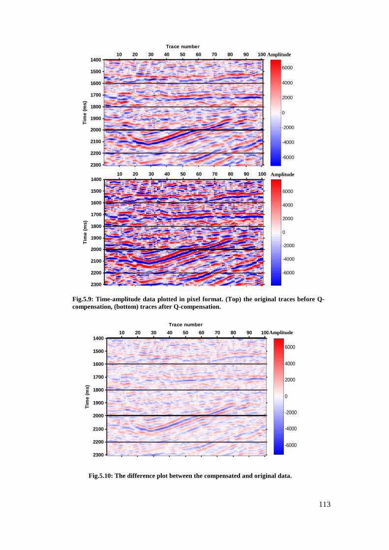
113
10 20 30 40 50 60 70 80 90 1001400
1500
1600
1700
1800
1900
2000
2100
2200
2300
Trace number
Tim
e (m
s)
-6000
-4000
-2000
0
2000
4000
6000
10 20 30 40 50 60 70 80 90 1001400
1500
1600
1700
1800
1900
2000
2100
2200
2300
Tim
e (m
s)
-6000
-4000
-2000
0
2000
4000
6000
10 20 30 40 50 60 70 80 90 1001400
1500
1600
1700
1800
1900
2000
2100
2200
2300
Trace number
Tim
e (m
s)
-6000
-4000
-2000
0
2000
4000
6000
Fig.5.9: Time-amplitude data plotted in pixel format. (Top) the original traces before Q-compensation, (bottom) traces after Q-compensation.
Fig.5.10: The difference plot between the compensated and original data.
Amplitude
Amplitude
Amplitude

114
5.6: Q-compensation and the input layer parameters The Q-compensation process described above, just like any other inverse Q
filtering scheme, assumes a priori information concerning the layer parameters.
Most important among these parameters (in this case) is the quality factor (Q).
The trueness of the resulting seismic image after attenuation compensation may
not only depend on the robustness of the compensation algorithm, but may also
depend on the accuracy of the estimated quality factor (or attenuation) that serve
as input into the Q-compensation scheme. Because the estimated values of Q
may be different from the real values of Q, we can express the error in a Q
estimate as:
�8 �� P ∆�. 5.12
Where �8, �� and ∆� are the estimated, actual, and error Q value respectively.
Here, the effects of incorrect Q on the Q-compensated seismic signals are
examined. The Earth model used for the synthetic experiment comprises of three
layers (figure 5.13): top shale; sandstone reservoir; and basal shale. Attenuation
in the sandstone reservoir is represented by 0.05 (Q = 20).
250m
200m
Inf.
Upper shale
sandstones
Lower shale
shaleshale
Fig. 5.11: A three layer Earth mode- sandstone reservoir between two shale layers.
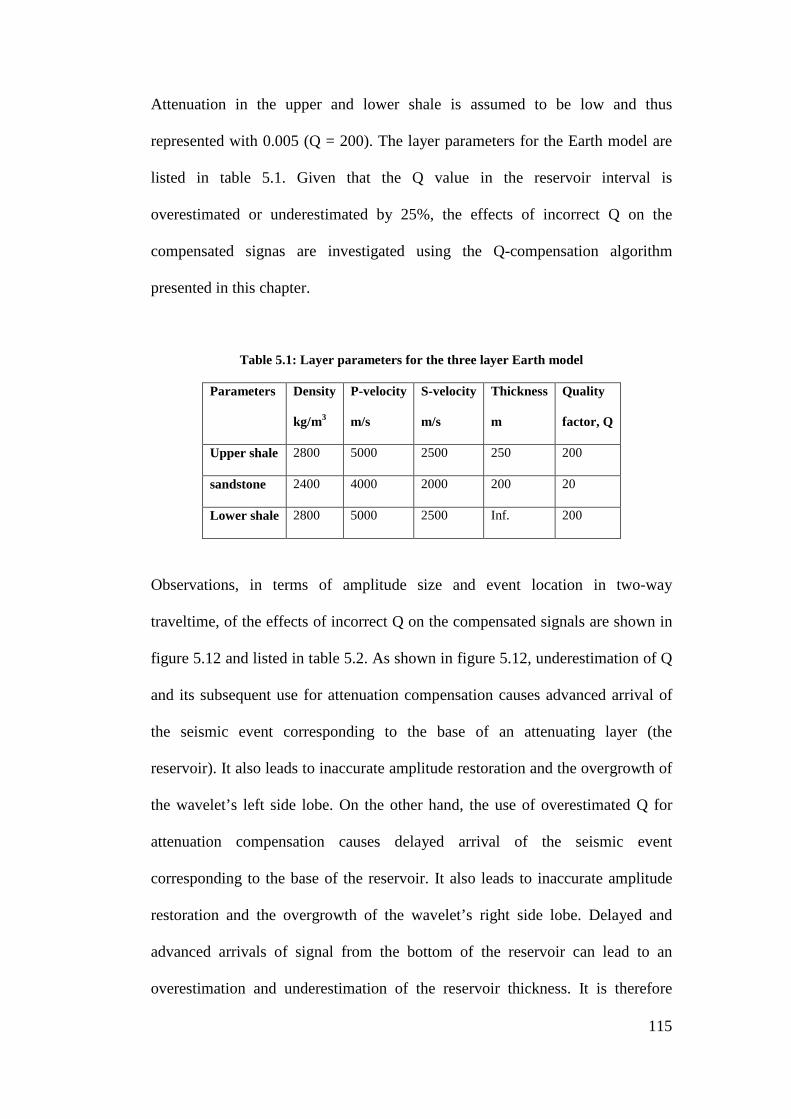
115
Attenuation in the upper and lower shale is assumed to be low and thus
represented with 0.005 (Q = 200). The layer parameters for the Earth model are
listed in table 5.1. Given that the Q value in the reservoir interval is
overestimated or underestimated by 25%, the effects of incorrect Q on the
compensated signas are investigated using the Q-compensation algorithm
presented in this chapter.
Table 5.1: Layer parameters for the three layer Earth model
Parameters
Density
kg/m3
P-velocity
m/s
S-velocity
m/s
Thickness
m
Quality
factor, Q
Upper shale 2800 5000 2500 250 200
sandstone 2400 4000 2000 200 20
Lower shale 2800 5000 2500 Inf. 200
Observations, in terms of amplitude size and event location in two-way
traveltime, of the effects of incorrect Q on the compensated signals are shown in
figure 5.12 and listed in table 5.2. As shown in figure 5.12, underestimation of Q
and its subsequent use for attenuation compensation causes advanced arrival of
the seismic event corresponding to the base of an attenuating layer (the
reservoir). It also leads to inaccurate amplitude restoration and the overgrowth of
the wavelet’s left side lobe. On the other hand, the use of overestimated Q for
attenuation compensation causes delayed arrival of the seismic event
corresponding to the base of the reservoir. It also leads to inaccurate amplitude
restoration and the overgrowth of the wavelet’s right side lobe. Delayed and
advanced arrivals of signal from the bottom of the reservoir can lead to an
overestimation and underestimation of the reservoir thickness. It is therefore
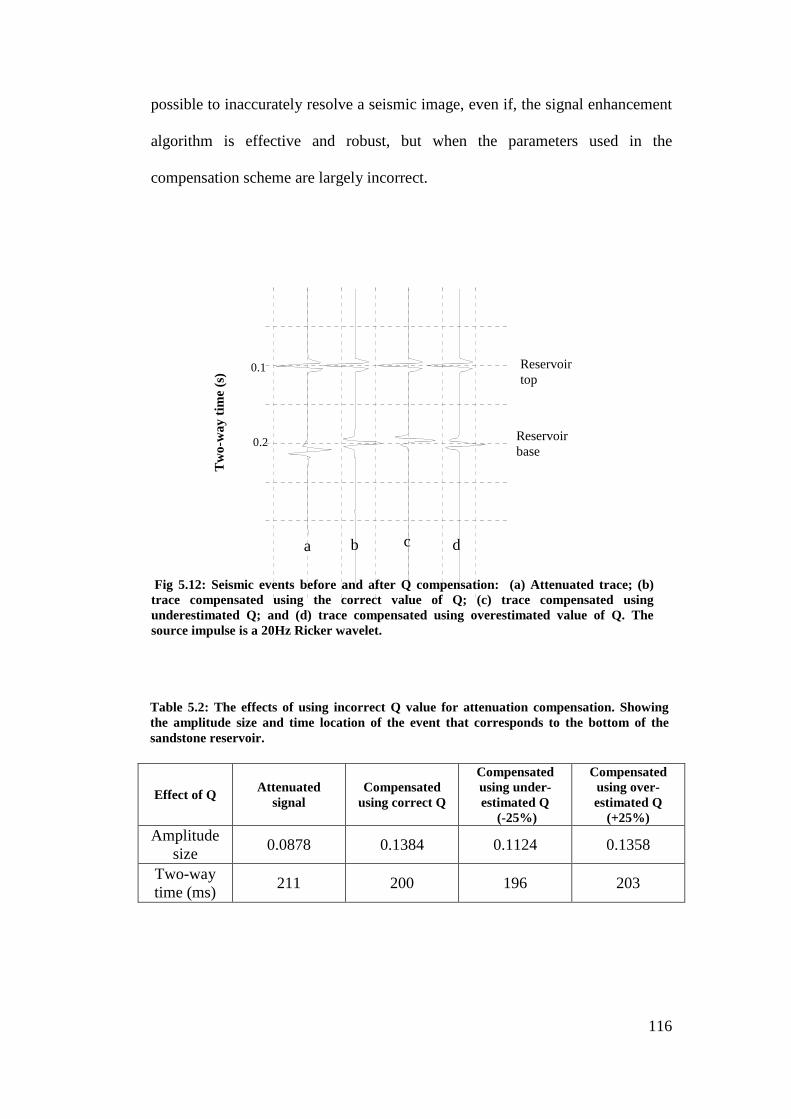
116
possible to inaccurately resolve a seismic image, even if, the signal enhancement
algorithm is effective and robust, but when the parameters used in the
compensation scheme are largely incorrect.
Effect of Q Attenuated
signal Compensated
using correct Q
Compensated using under- estimated Q
(-25%)
Compensated using over- estimated Q
(+25%) Amplitude
size 0.0878 0.1384 0.1124 0.1358
Two-way time (ms)
211 200 196 203
Fig 5.12: Seismic events before and after Q compensation: (a) Attenuated trace; (b) trace compensated using the correct value of Q; (c) trace compensated using underestimated Q; and (d) trace compensated using overestimated value of Q. The source impulse is a 20Hz Ricker wavelet.
Table 5.2: The effects of using incorrect Q value for attenuation compensation. Showing the amplitude size and time location of the event that corresponds to the bottom of the sandstone reservoir.
Reservoir top
Reservoir base
a b c d
Tw
o-w
ay ti
me
(s) 0.1
0.2
117
5.7: Discussion
Seismic wave propagation in real Earth is different in many ways from wave
propagation in an ideal solid. The Earth is neither a perfectly elastic medium nor
an ideal solid medium. The amplitude, waveform, and arrival time of waves
propagating in the Earth are influenced by anelasticity and inhomogeneity in the
rocks through which they travel. This causes attenuation which degrades the
quality of seismic data and affects the resolution of subsurface structures. An
efficient method of correcting the undesirable effects of the Earth’s attenuation
on seismic waves is described in this chapter. For a single layer, the scheme is
basically an inverse procedure for the wave propagation. The procedure is similar
to starting from the receiver, backward-propagate the wave to the reflector and to
the source. For seismic records from a stack of layers, the Q-compensation
scheme is implemented in a layer by layer recursive manner. The attenuated
signal corresponding to each lithology or seismic layer is treated with the Q
responsible for the attenuation and dispersion using an inverse Q filter. By this
approach, every seismic event is treated for attenuation and dispersion it
experienced along its propagation path. The applications of the Q-compensated
algorithm to synthetic and field seismic data show that the algorithm is
appropriate for correcting amplitude diminution and phase dispersion in seismic
waves, and thus improves the interpretability of seismic records. Synthetic
experiments on the effects of using incorrect Q for attenuation compensation
shows that largely incorrectly estimated attenuation and its subsequent use for
attenuation compensation can lead to inaccurate amplitude restoration and under-
correction of dispersion. The Q-compensated scheme described in this chapter
118
can be incorporated into a migration scheme to achieve a well resolved migrated
image.
5.8: Conclusion
An algorithm for correcting the effects of amplitude diminution, wavelet
distortion and velocity dispersion in seismic waves has been presented. The Q-
compensation scheme circumvents the undesirable effects of instability and
prevents the introduction of artefacts that usually mar the results of an inverse Q-
filtering process. The method proved appropriate when applied to synthetic and
field seismic data. The Q-compensation process improves the quality of seismic
images and returns subsurface reflectors to their correct position, by correcting
amplitude diminution, waveform distortion and phase delay. The process
generally improves the interpretability of the seismic section. The use of an
incorrect Q in a compensation scheme affects the quality of the compensated
seismic images. Therefore, the quality of a Q-compensated seismic record
depends on the robustness of the compensation algorithm and the accurateness of
the input parameters.

119
Chapter Six
THE USE OF SEISMIC ATTENUATION FOR MONITORING
SATURATION IN HYDROCARBON RESERVOIRS
120
6.1: Summary
A theoretical rock physics forward model and synthetic time lapse seismic data
have been used to explore the possible use of attenuation to monitor saturation in
hydrocarbon reservoirs. Given the time variant changes in saturation and the
properties of the reservoir rock, the rock physics anelastic model (Mavko et al.
1998) is used to formulate a theoretical curve to observe the dynamic effects of
saturation on attenuation. The partial saturation part of the curve is used to
formulate a relation between attenuation and saturation. Attenuation is measured
in time lapse synthetic seismic records and the curve-based relation is used to
estimate the approximate corresponding saturation that gave rise to the
seismogram-derived attenuation (SDA). Results from the study show that SDA
can be used to monitor hydrocarbon saturation in reservoirs, if a relationship
between SDA and saturation is known; the saturation values predicted by the
theoretical model are consistent with the saturation values inverted from SDA.
Apart from saturation, attenuation depends on porosity, mineral content of the
rock, and the property of the saturating fluid(s). For the case studied, at a
saturation of 0.7, a 10% reduction in porosity caused a 5.9% rise in attenuation,
while a 10% reduction in the bulk modulus of the saturating fluids caused an
11% reduction in attenuation.
6.2: Introduction
The observed changes in amplitude and frequency content of seismic signals
recorded from a reservoir rock as its saturation changes make it theoretically
plausible to use attenuation measured in seismic data (SDA) to monitor or predict
saturation in hydrocarbon reservoirs; however, a relation between SDA and
121
saturation is still unknown. Attenuation is a propagational seismic attribute that
can be measured in seismic records and well log data. A detailed knowledge of
attenuation is beneficial for seismic data processing and pore fluid
discrimination. The low frequency shadow associating with attenuation has been
exploited to identify hydrocarbon saturated layers (Castagna et al., 2003;
Singleton, 2008). A combination of P- and S-waves attenuation and P- and S-
wave velocity ratio has been applied to discriminate gas sand from oil sand and
oil sand from water sand (Klimentos, 1995). Despite the compelling evidence
from laboratory and theoretical studies (Mavko et al., 1998; Cadoret, 1995;
Muller and Gurevich, 2004) that increase in saturation (up to a critical saturation
level) will cause increase in seismic attenuation, predicting saturation from SDA
is still a difficult endeavour. The increase in reservoir saturation with time can
be observed in time lapse saturation logs. Saturation values obtained from well
logs can be combined with the elastic rock moduli using Gassmann’s (1951)
equation and the standard linear solid model (Mavko et al., 1998), to create the
attenuation-saturation character curve for the rock under investigation. The
increase in reservoir saturation will affect the amplitude, frequency content, and
travel time of a wave travelling through the reservoir. Therefore, the effects of
changes in saturation should be measurable in seismic waveforms in terms of
attenuation. Amplitude diminution and frequency down-shift in waves are foot
prints of attenuation and they have been used to measure attenuation in seismic
records (e.g., Dasgupta and Clark, 1998; Rein et al. 2009). If scattering
attenuation is removed from SDA, the theoretical curve can be used to invert the
saturation that gave rise to seismic attenuation.
122
The patchy saturation model is commonly used to explain the physical
phenomenon that causes seismic attenuation in waves travelling in an isotropic
porous medium containing two or more fluids. The phenomenon is explained by
the movement of fluids with low compressibility (e.g., water) into and out of
space accommodating a more compressible fluid (e.g., gas) due to the changes in
pressure created by the passage of seismic waves. The process causes attenuation
because some energy of the passing wave is irreversibly converted to heat during
the movement of fluid in and out of confined rock pore structure. The patchy
saturation model plausibly describes the volumetric disposition of fluids having
different compressibilities (Mavko et al., 1998) and is suitable for describing the
mechanism of attenuation in reservoir rock that usually contains two or more
saturants (e.g., water, oil or gas). The theory of modulus-frequency-dispersion
typically describes the dynamic effect of saturation on attenuation in porous
isotropic media containing two or more fluids(Raji and Rietbrock, 2012). The
model has been applied to the study of attenuation in real hydrocarbon reservoirs
(Dvorkin and Uden, 2004; Dvorkin and Mavko, 2006). I adopt the patchy
saturation mechanism and used the theory of modulus-frequency dispersion to
study the effect of changes in saturation on seismic wave attenuation. The
assumptions in the study are as follows: (i) Saturation is the sole cause of the
attenuation measured in seismic data. (ii) The theoretical curve from the
modulus-frequency-dispersion describes the approximate relation between
attenuation and saturation for the rock model under study. The study builds on
the theoretical description of the effects of saturation on attenuation using the
theory of modulus-frequency-dispersion (Mavko et al., 1998) and attenuation
measurement in field and synthetic seismic records.
123
6.3: The use of seismogram-derived attenuation (SDA) for monitoring reservoir saturation
Patchy saturation model is known to be the principal process responsible for
attenuation and dispersion in seismic waves at frequencies similar to those used
in seismic exploration (Pride et al., 2004). I adopt the patchy saturation
mechanism, and applied the theory of modulus-frequency-dispersion to observe
the dynamic effect of saturation on attenuation. A modelled but realistic reservoir
rock used for this study consists of two parts: the patches, and the background
rock matrix, each saturated with water and gas respectively. The properties of the
reservoir rock and their numeric values are detailed in appendix 6. The effect of
pore fluid changes on the elastic moduli of the rock is estimated using the rock
properties that can be obtained from well log data and laboratory measurements,
and related by rock physics formulation (Gassmann, 1951). Attenuation is related
to the rock moduli versus frequency using the Krammer-Kronig relation and the
standard linear model (Mavko et al., 1998) as:
��o,�� &z� @ z(� 2©z�z(⁄ , 6. 1
where z� is the high frequency compressional moduli, z( is the low frequency
compressional moduli and ��o,�� is the maximum inverse quality factor. At low
frequency, the effective pore fluid is the mixture of water and gas at pore scale.
The bulk modulus of the fluid is the harmonic average of the moduli of water and
gas (Dvorkin et al., 2003). The bulk modulus of the partially saturated rock is
estimated using Gassmann (1951) formulation while the compressional modulus
of the partially saturated rock is estimated as:
z( �( P �� �Ô�ý, 6.2
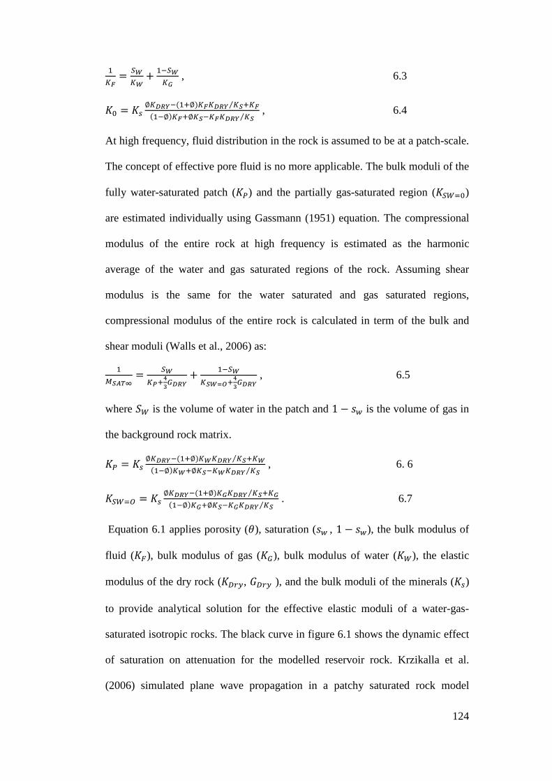
124
��� ���� P ������ , 6.3
�( �j y�����&�~y������� �#⁄ ~��&��y���~y�#������� �#⁄ , 6.4
At high frequency, fluid distribution in the rock is assumed to be at a patch-scale.
The concept of effective pore fluid is no more applicable. The bulk moduli of the
fully water-saturated patch (��) and the partially gas-saturated region (����()
are estimated individually using Gassmann (1951) equation. The compressional
modulus of the entire rock at high frequency is estimated as the harmonic
average of the water and gas saturated regions of the rock. Assuming shear
modulus is the same for the water saturated and gas saturated regions,
compressional modulus of the entire rock is calculated in term of the bulk and
shear moduli (Walls et al., 2006) as:
�{#¶·| ��� ~������ P �����#� ¡~������ , 6.5
where �� is the volume of water in the patch and 1 @ ¢+ is the volume of gas in
the background rock matrix.
�� �j y�����&�~y������� �#⁄ ~��&��y���~y�#������� �#⁄ , 6. 6
����£ �j y�����&�~y������� �#⁄ ~��&��y���~y�#������� �#⁄ . 6.7
Equation 6.1 applies porosity (â), saturation (¢+ , 1 @ ¢+), the bulk modulus of
fluid (�°), bulk modulus of gas (��), bulk modulus of water (��), the elastic
modulus of the dry rock (���, ��� ), and the bulk moduli of the minerals (�j)
to provide analytical solution for the effective elastic moduli of a water-gas-
saturated isotropic rocks. The black curve in figure 6.1 shows the dynamic effect
of saturation on attenuation for the modelled reservoir rock. Krzikalla et al.
(2006) simulated plane wave propagation in a patchy saturated rock model
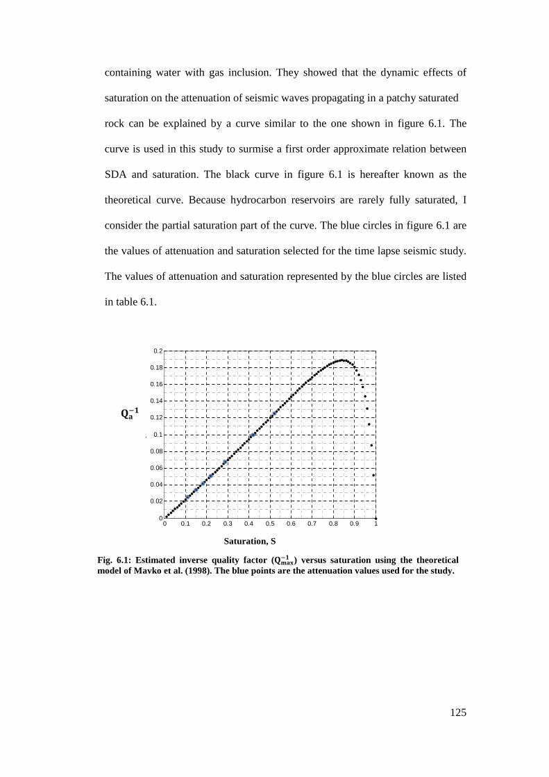
125
containing water with gas inclusion. They showed that the dynamic effects of
saturation on the attenuation of seismic waves propagating in a patchy saturated
rock can be explained by a curve similar to the one shown in figure 6.1. The
curve is used in this study to surmise a first order approximate relation between
SDA and saturation. The black curve in figure 6.1 is hereafter known as the
theoretical curve. Because hydrocarbon reservoirs are rarely fully saturated, I
consider the partial saturation part of the curve. The blue circles in figure 6.1 are
the values of attenuation and saturation selected for the time lapse seismic study.
The values of attenuation and saturation represented by the blue circles are listed
in table 6.1.
����
Fig. 6.1: Estimated inverse quality factor (������ ) versus saturation using the theoretical model of Mavko et al. (1998). The blue points are the attenuation values used for the study.
0 0.1 0.2 0.3 0.4 0.5 0.6 0.7 0.8 0.9 10
0.02
0.04
0.06
0.08
0.1
0.12
0.14
0.16
0.18
0.2
Q1
saturation
Saturation, S
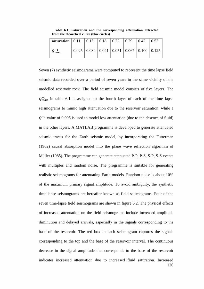
126
saturation 0.11 0.15 0.18 0.22 0.29 0.42 0.52
¨´¦µ�� 0.025 0.034 0.041 0.051 0.067 0.100 0.125
Seven (7) synthetic seismograms were computed to represent the time lapse field
seismic data recorded over a period of seven years in the same vicinity of the
modelled reservoir rock. The field seismic model consists of five layers. The
��o,�� in table 6.1 is assigned to the fourth layer of each of the time lapse
seismograms to mimic high attenuation due to the reservoir saturation, while a
��� value of 0.005 is used to model low attenuation (due to the absence of fluid)
in the other layers. A MATLAB programme is developed to generate attenuated
seismic traces for the Earth seismic model, by incorporating the Futterman
(1962) causal absorption model into the plane wave reflection algorithm of
Müller (1985). The programme can generate attenuated P-P, P-S, S-P, S-S events
with multiples and random noise. The programme is suitable for generating
realistic seismograms for attenuating Earth models. Random noise is about 10%
of the maximum primary signal amplitude. To avoid ambiguity, the synthetic
time-lapse seismograms are hereafter known as field seismograms. Four of the
seven time-lapse field seismograms are shown in figure 6.2. The physical effects
of increased attenuation on the field seismograms include increased amplitude
diminution and delayed arrivals, especially in the signals corresponding to the
base of the reservoir. The red box in each seismogram captures the signals
corresponding to the top and the base of the reservoir interval. The continuous
decrease in the signal amplitude that corresponds to the base of the reservoir
indicates increased attenuation due to increased fluid saturation. Increased
Table 6.1: Saturation and the corresponding attenuation extracted from the theoretical curve (blue circles)
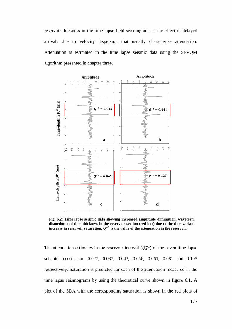
127
reservoir thickness in the time-lapse field seismograms is the effect of delayed
arrivals due to velocity dispersion that usually characterise attenuation.
Attenuation is estimated in the time lapse seismic data using the SFVQM
algorithm presented in chapter three.
The attenuation estimates in the reservoir interval (�o��) of the seven time-lapse
seismic records are 0.027, 0.037, 0.043, 0.056, 0.061, 0.081 and 0.105
respectively. Saturation is predicted for each of the attenuation measured in the
time lapse seismograms by using the theoretical curve shown in figure 6.1. A
plot of the SDA with the corresponding saturation is shown in the red plots of
01
23
45
67
-0.4
-0.3
-0.2
-0.1 0
0.1
0.2
0.3
0.4 01
23
45
67
-0.4
-0.3
-0.2
-0.1 0
0.1
0.2
0.3
0.4Q
=20
01
23
45
67
-0.4
-0.3
-0.2
-0.1 0
0.1
0.2
0.3
0.4 01
23
45
67
-0.4
-0.3
-0.2
-0.1 0
0.1
0.2
0.3
0.4
Fig. 6.2: Time lapse seismic data showing increased amplitude diminution, waveform distortion and time-thickness in the reservoir section (red box) due to the time-variant increase in reservoir saturation. ��� is the value of the attenuation in the reservoir.
¨�� þ. þ�� ¨�� þ. þ��
¨�� þ. þ�� ¨�� þ. ���
Tim
e-de
pth
x102
(ms)
T
ime-
dept
h x1
02 (m
s)
d c
a b
Amplitude Amplitude

128
figure 6.3. The saturation equivalence of the seismic derived attenuation, SDA
(red circles) can be obtained by tracing each red point to the abscissa (X-
coordinate).
Attenuation estimates from seismic data is usually influenced by many factors.
These factors include the presence of seismic noise, thin layering effects, data
processing method, and the appropriateness of the attenuation measuring
algorithm. These factors can in turn affect saturation that is predicted from SDA.
The attenuation estimates for the highest input saturation (indicated by the red
arrows) in figure 6.3 significantly differ from the input model (the blue circles
indicated by the blue arrows). This is because (i) the attenuation measuring
algorithm is less reliable for predicting attenuation when the ��� model � 0.10;
(ii) the effects of seismic noise is very high - the amplitude of the signal
corresponding to the base of the reservoir has been drastically reduced by
attenuation and the noise is now about the size of the desired seismic signal (see
figure 6.2d). The influence of the two factors mentioned in (i) and (ii) caused
significant error in the saturation predicted from the attenuation measured in the
field seismogram. To reduce the uncertainty in saturation estimates due to the
effect of noise on attenuation measurements, the seismic data can be treated for
noise by a frequency-neutral algorithm such that the process of de-noising does
not affect the frequency profile of the primary signals. In this case, the effect of
noise on attenuation measurement is reduced by measuring attenuation in noise
free synthetic seismograms in addition to the one measured in the field
seismograms. Synthetic noise-free seismograms are generated for each of the

129
time lapse seismic data using the MATLAB programme described earlier.
Attenuation estimates in the reservoir section of the noise-free synthetic
seismograms (�G��) are 0.023, 0.033, 0.040, 0.053, 0.069, 0.105 and 0.151,
respectively. To reduce the uncertainties in saturation estimates due to the effect
of noise on attenuation measurement, saturation is predicted from the mean
attenuation (����). The mean attenuation is computed as the average of �o�� and
�G��. The plot of ���� and the corresponding saturation is shown in figure 6.4.
The saturation values inverted from the SDA after correcting for the effect of
noise («¨«) (red circles in Fig. 6.4) and the saturation predicted by the theoretical
model «¨¤ (the circles plots in Fig. 6.4) are compared in table 6.2. Reducing the
effects of noise on attenuation measurement shows significant improvement in
the saturation estimates, the saturation values predicted from SDA after reducing
0 0.1 0.2 0.3 0.4 0.5 0.6 0.7 0.8 0.9 10
0.05
0.1
0.15
0.2
0.25
0.3
Fig. 6.3: Seismogram-derived attenuation plotted with saturation (red circles). Saturation is inverted from the SDA using the theoretical curve. The black circles are the plots of attenuation and saturation from the theoretical curve in figure 6.1.
Saturation, S
����

130
the effect of noise are more consistent with the saturation computed using the
theoretical model.
���
0.11 0.15 0.18 0.22 0.29 0.42 0.52
��� 0.11 0.15 0.18 0.23 0.30 0.39 0.54
6.4: Effects of other reservoir properties on attenuation
Apart from saturation level, attenuation depends on other properties of the rock
and fluid. These factors include porosity and mineral composition of the rock
0 0.1 0.2 0.3 0.4 0.5 0.6 0.7 0.8 0.9 10
0.05
0.1
0.15
0.2
0.25
0.3
���
Saturation
Fig. 6.4: Seismogram-derived attenuation after reducing the effects of noise plotted with saturation (red plots). Saturation is inverted from the SDA using the theoretical curve. The blue circles are the plot of attenuation and saturation from figure 6.1.
Table 6.2: Saturation values predicted for the seismic derived attenuation (���) and the theoretical rock physics model (���)
131
(Winkler and Nur, 1982; Klimentos and McCann, 1990) , the compressibility and
viscosity of the fluid (Chapman et al., 2003; Muller and Gurevich, 2004), and
temperature (Faul and Jackson, 2005; Fontaine et al., 2005). Attenuation
estimates in seismic records also can be influenced by thin layer effects and the
presence of noise.
To study the influence of other material properties of rock on attenuation, I kept
saturation constant and perturb the porosity, the bulk modulus of the fluids, and
the mineral composition of the rock, one after the other by 10%, in contrast to the
values used in figure 6.1 (black dots). Figure 6.5 shows the effects of these
parameters on attenuation predicted by the theoretical model. The green plot
shows the effects of 10% reduction in porosity; the blue plot is the effect of
altering the mineral composition- reducing the quartz composition by 10% and
increasing clay composition by 10%; and the red plot shows the effects of
reducing the modulus of the fluid by 10%. I found that the change in mineral
composition has the least effects on attenuation - the blue curve almost
completely overlaid the theoretical (black) curve. At 0.17 attenuation (��o,�� ) and
70% saturation (shown in black horizontal and vertical lines in figure 6.5), the
10% reduction in porosity increased attenuation by 5.9%, while a 10% reduction
in the fluid moduli caused 11% decrease in attenuation. The tuning effects due to
thin layers causes scattering attenuation and it can influence the magnitude of
attenuation estimated in seismic data. When the thickness of an attenuating layer
is less than a quarter of the dominant wavelength, the layer is known as thin
layer. In thin layers, the wavelets of the incident and transmitted signals become
undistinguishable, making it difficult to reliably compute the signal spectra
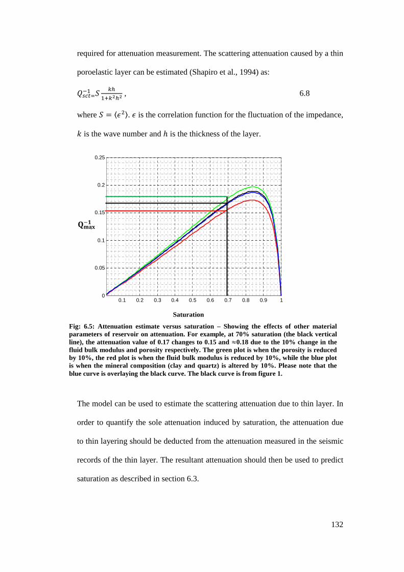
132
required for attenuation measurement. The scattering attenuation caused by a thin
poroelastic layer can be estimated (Shapiro et al., 1994) as:
�jNH��� � �ã�~�\ã\ , 6.8
where � p�6r. � is the correlation function for the fluctuation of the impedance,
C is the wave number and ¾ is the thickness of the layer.
The model can be used to estimate the scattering attenuation due to thin layer. In
order to quantify the sole attenuation induced by saturation, the attenuation due
to thin layering should be deducted from the attenuation measured in the seismic
records of the thin layer. The resultant attenuation should then be used to predict
saturation as described in section 6.3.
0.1 0.2 0.3 0.4 0.5 0.6 0.7 0.8 0.9 10
0.05
0.1
0.15
0.2
0.25
saturation
Q1
Fig: 6.5: Attenuation estimate versus saturation – Showing the effects of other material parameters of reservoir on attenuation. For example, at 70% saturation (the black vertical line), the attenuation value of 0.17 changes to 0.15 and �0.18 due to the 10% change in the fluid bulk modulus and porosity respectively. The green plot is when the porosity is reduced by 10%, the red plot is when the fluid bulk modulus is reduced by 10%, while the blue plot is when the mineral composition (clay and quartz) is altered by 10%. Please note that the blue curve is overlaying the black curve. The black curve is from figure 1.
������
Saturation
133
The emphasis of this section is that an x degree of saturation can cause different
magnitude of attenuation in different rocks due to the variation in other material
properties. Depth of burial, effects of overburden materials and temperature may
cause variation in porosity and mineral composition of reservoirs found at
different depths, it is possible that reservoir rocks found in the same area but at
different depths, can have different attenuation, even if, they have similar
saturation. It also follows that different attenuation values may be measured in
seismic data recorded from two reservoir rocks having similar material properties
and saturation but different thicknesses. It is therefore important to note that
every attenuation–saturation case should be treated individually based on the
properties and saturation conditions of the rocks. Separate theoretical curves
should be computed for different rocks, and the theoretical curve should be used
to invert saturation for the attenuation measured in seismic data after removing
the contribution of scattering attenuation.
6.5: Attenuation calibration: seismic to well logs
Reliable estimates of seismic attenuation is beneficial for seismic processing,
saturation indication and indirect signs of pore structure (Mittet et al., 1995,
Winkler and Nur, 1982; Klimentos, 1995). To use attenuation data for
exploration purposes, a check on the validity of attenuation measured in field
data is necessary. One possible way of doing this check is to measure attenuation
from two or more independent data sources, such as well log and seismic data
recorded in the same vicinity. Attenuation can be measured in well log data using
the heterogeneous Q model (Dvorkin and Uden, 2004; Dvorkin and Mavko,

134
2006) and in field seismograms using various methods (e.g., Quan and Harris,
1997; Dasgupta and Clark, 1998; Zang and Ulrych, 2002; Clark et al., 2009).
Comparison of attenuation data obtained from different data sources can be used
to produce a well constrained attenuation profile that will be beneficial to
exploration, specifically, to indicate the extent of a potential hydrocarbon pay
zone. The limitation in comparing attenuation data obtained from well logs and
seismic data is that the values of attenuation measured from the two sources of
data recorded in the same vicinity are usually not the same. The procedure
required to calibrate the attenuation measured in well log data to the one
measured in seismic data is the subject of this section. To calibrate the seismic-
derived attenuation to the well logs-derived attenuation, I assumed that the
attenuation measured from recorded well logs is solely the intrinsic attenuation.
On the other hand, the attenuation measured from seismic records is a composite
attenuation that consists of both the intrinsic and extrinsic attenuation. Because
of this, the composite attenuation measured in field seismic data should be
reduced to intrinsic attenuation. Seismic signals will always show signs of
attenuation due to (stratigraphic) scattering energy loss from the geometric
arrangement of layers, even if the Earth model is elastic. The energy loss in this
case is not dissipated into heat but will arrive later in time or be part of the
unobserved wave field. The energy loss due to tuning effect of thin layer is
another form of extrinsic attenuation. The total extrinsic attenuation can then be
estimated as the sum of the losses due to stratigraphic attenuation (����) and the
thin layering effects (�6��) as:
�8,�� ���� P �6��. 6. 9

135
The intrinsic attenuation is then estimated from the seismic field data as the
difference between the composite attenuation and the extrinsic attenuation using
the additive law of attenuation (Dainty, 1981; Richard and Menke, 1983; Mayeda
et al., 1992; Ik Bum and McMechan, 1994) as:
��� � ���ú P ��¸Ó�. 6.10
The intrinsic attenuation estimated from field seismic data as shown in equation
6.10 can then be equated to the attenuation measured in recorded well-logs, at
corresponding intervals, to obtain a calibration ratio.
6.6: Discussion and Conclusion
Theoretical but realistic rock physics model is applied to study the attenuation
dependence on saturation. The relationship observed in the theoretical curve is
used to describe the saturation dependence of seismic attenuation for the
modelled reservoir rock. Attenuation measured in seismic records is input into
the theoretical curve to invert the saturation equivalence for SDA. Because of the
strategic importance of attenuation to geophysical reservoir characterisation, a
procedure for calibrating seismic-derived attenuation to the borehole-derived
attenuation is also described. The calibration is a useful check for comparing the
trend in the attenuation measured from two sources of data, at corresponding
depth intervals, to reduce uncertainties in Q measurements and its interpretation.
The higher the attenuation measured in seismic records, the higher the saturation
inverted from SDA. The results show that the time variant saturation increase in
reservoir rocks can cause increased seismic wave attenuation that is measureable

136
in time lapse seismic data, and that attenuation can be used to monitor saturation
in reservoir rocks. If the relationship between attenuation and saturation is
known, attenuation measured in seismic records can be used to a first order
approximation, to predict hydrocarbon saturation in reservoirs. Aside saturation,
attenuation depends on some material properties of rocks. These properties affect
the magnitude of attenuation estimated using rock physics theoretical model and
the saturation predicted from the curve. For the case study, a 10% reduction in
porosity caused a 5.9% rise in attenuation, while a 10% reduction in the bulk
modulus of the saturating fluids caused an 11% drop in attenuation. These
changes have corresponding effects on the saturation predicted from the
attenuation.

137
Chapter Seven
SUMMARY OF RESULTS
138
7.1: Discussion and Summary of results
The work presented in this thesis covers four aspects of seismic attenuation
research: (i) attenuation measurement in seismic data; (ii) estimation of P- and S-
wave attenuation in recorded well logs; (iii) attenuation analysis for pore fluid
determination; (iv) and attenuation compensation in seismic data. Where
applicable, 3D seismic or well log data recorded in the Gullfaks field, North Sea,
Norway, was used to test the model or algorithm developed in this thesis. The
results from the study are discussed chapter by chapter.
Chapter three
Determination of quality factor (Q) in reflection seismic data
A new method (SFVQM) for measuring attenuation in reflection seismic data is
presented. The technique is based on the difference in the centroid frequency of
paired seismic events, their traveltime difference, and a spectral shape factor. The
inversion process involves two key stages: computation of the centroid frequency
for the individual seismic signal using variable window length and fast Fourier
transform; and estimation of the difference in the centroid frequencies and
traveltimes for a pair of incident and transmitted signals. The use of a shape
factor in the formulation made it possible to represent the real seismic signal by
any spectral shape that satisfies the basic characteristic of a real seismic signal.
Compared to the method that uses the peak frequency (Zhang and Ulrych, 2002)
or the entire frequency bandwidth (Bath, 1974; Spencer et al., 1982), SFVQM is
less sensitive to noise interference and change of frequency bandwidth. SFVQM
is tested for attenuation measurement in synthetic and real seismic data. In the
case of real data, the trace length is partitioned into four intervals, and Q is

139
measured in the traces one after the other. The distribution of Q estimates within
the four intervals is shown by histograms. Furthermore, the mean attenuation
(1/��) and its standard deviation are computed. Finally, 1D attenuation profiles
are plotted from the attenuation estimates. The main results are summarised
below:
• Tests on synthetic data show that SFVQM can provide reliable estimates
of Q using either a Ricker, an Ormsby, a triangular, or a Gaussian wavelet
to represent the real seismic signal. The maximum difference in the Q
estimates using any of the wavelets is about 5% when the Q value in the
Earth model ranges from 10 to 50. The difference increased to 12% when
the Q value in the Earth model is 100;
• In comparison with the spectral ratio method (Bath, 1974; Spencer, 1982)
and the method proposed by Quan and Harris (1997), SFVQM shows less
sensitivity to noise interference and change of frequency bandwidth. The
error in the Q estimates due to noise interference is 9.5% for SFVQM and
13.4% for the spectral ratio method. The errors due to change of
frequency bandwidth are 9.8% and 14.7%, for the SFVQM and the
method of Quan and Harris (1997), respectively;
• For the purposes of attenuation measurement, the field data is partitioned
into four intervals: AB, BC, CD, and DE. The mean attenuation 1/Q
calculated from 500 measurements in the four intervals are 0.0196,
140
0.0573, 0.0389, and 0.0220 respectively. Their corresponding standard
deviations are 0.0045, 0.0338, 0.0180, and 0.0075;
• The close agreement in the 1/Q values measured in the traces stacked
along CDP 602 line, using SFVQM and the spectral ratio method, shows
that SFVQM is appropriate for determining attenuation in seismic data.
This is further corroborated by the findings of Stainsby and Worthington
(1985) after measuring attenuation in VSP data recorded in a well from
the North Sea, Norway;
• The composite attenuation measured in seismic data is separated into
intrinsic and scattering attenuation using the additive law (Spencer et al.,
1982; Richard and Menke, 1983). In the case presented, the intrinsic
attenuation dominates the composite attenuation.
Chapter four
Rock physics diagnostics, attenuation measurement and analyses in wells
Chapter four presents an application of the elastic modulus and the visco-elastic
attenuation to study fluids in rocks. The bulk modulus, shear modulus,
compressional modulus, and Lame’s first parameter are estimated in the rocks
penetrated by well A-10 of the Gullfaks field. The theories of modulus-
frequency-dispersion and the standard linear model (Mavko et al., 1998; Dvorkin
and Uden, 2004) were applied to estimate attenuation in the well log data. P- and
S-wave attenuation pseudo-logs were computed for the logged interval, and a

141
cross analysis of the velocity and attenuation ratios was used to discriminate gas
from water and water from oil. The chapter applied some quantitative models to
compute some missing data in the log suite. Results from the study are
summarised below:
• Lame’s first parameter, bulk modulus, and compressional modulus show
comparable sensitivities to pore fluids. They are lower in gas-saturated
rock compared to water-saturated rock, and higher in oil-saturated rock
compared to water-saturated rock. The shear modulus does not show
sensitivity to pore fluids;
• The P-wave inverse quality factor (����) is higher in hydrocarbon-
saturated rocks than in water saturated rocks. The values of the ratio of P-
to S-wave attenuation (� !"�#!") measured in gas, water, and oil-saturated
rocks are 0.57 - 0.78, 0.39 - 0.55, and 0.35 - 0.41, respectively;
• A cross analysis of the velocity and the attenuation factor clearly
distinguishes gas from water and water from oil. Gas sand is
characterized by the highest � !"�#!" and the lowest
$ $# values; oil sand is
characterized by the lowest � !"�#!" and the highest
$ $# values; and water sand
is characterized by � !"�#!" and
$ $# values between those of the gas sand and
oil sand.
142
Chapter five
Enhanced seismic Q-compensation
To correct the undesirable effects of attenuation in recorded seismograms, an
enhanced Q-compensation algorithm is proposed. The Q-compensation scheme
is an inverse filtering process incorporating the attenuation (Q) factor. To
overcome the instability problem of conventional inverse Q-filters, wave
numbers are replaced with slowness, and the compensation scheme is
implemented in a layer-by-layer recursive process. The algorithm is tested with
synthetic and field seismic data, and found to be appropriate for correcting the
undesirable effects of attenuation. The improvements in the compensated data in
comparison with the original data are discussed below:
• Tests on synthetic seismograms show that the compensation algorithm
can be used to correct amplitude diminution and waveform distortion in
seismograms computed from any Earth Q model. The compensated
synthetic seismograms compares favourably with the seismograms
generated from an elastic Earth model;
• The compensated field data show clearer images of the subsurface
reflectors and higher amplitudes, compared with the original field data.
The average frequency spectrum of the compensated data contains high
frequency components (80-125Hz) that were absent in the original field
data.
143
• Generally, the compensation process enhanced the interpretability of the
synthetic and field data.
Chapter six
Predicting reservoir material parameter from attenuation
A theoretical curve describing the dynamic effect of saturation on attenuation is
computed, using the theory of modulus-frequency-dispersion and the properties
of the rock under investigation. Attenuation measured in synthetic time-lapse
seismograms is input to the theoretical curve to invert the saturation that caused
the attenuation observed in the seismograms. The findings show that attenuation
measured in seismograms can be used to invert saturation if a relation between
seismogram-derived attenuation and saturation is known. To study the effects of
other material parameters of rocks on attenuation, saturation is fixed while
porosity, mineral composition, and the bulk modulus of the fluid are perturbed,
one after the other, by 10%. A procedure for calibrating the attenuation measured
in seismic data to the attenuation measured in well log data is also discussed.
• The increase in saturation of a reservoir rock affects the amplitude and
frequency of a wave travelling through the rock, and thus the attenuation
experienced by the wave. Therefore, saturation can be predicted from
attenuation if a realistic relation between seismogram-derived attenuation
and saturation is known.
• The presence of noise can influence the accuracy of the attenuation
measured in seismic data, and therefore, influence the value of saturation
144
predicted from the attenuation-saturation curve. Correcting for the effect
of noise in the measured attenuation shows significant improvement in
the saturation values predicted by the curve.
• Aside from saturation, attenuation depends on a number of material
properties of rocks. These properties include porosity, the fluid bulk
modulus, and the mineral content of the rock. A 10% reduction in the
bulk modulus of the fluid causes an 11% decrease in attenuation; a 10%
reduction in porosity causes a 5.9% increase in attenuation; and a 10%
change in mineral content of the rock does not produce significant change
in attenuation. A certain degree of saturation can cause a different
magnitude of attenuation in different rocks, due to the difference in the
material properties of the rocks.
7.2: Future work
Standard amplitude-versus-offset (AVO) analysis typically ignores attenuation,
making use of purely elastic reflectivity modelling. Studies (e.g., Samec and
Blangy, 1992; Adriansyah and McMechan, 1998) have shown that attenuation
affects reflectivity with offset. Therefore, attenuation can influence AVO
signatures at the top and base of gas sand. Bourbie (1982) and Samec and
Blangy, (1992) studied the effects of attenuation on AVO signature at the base of
gas sand using reflectivity. They assumed an Earth model that comprises two
elastic layers encasing an attenuating gas sand layer. Their findings show how

145
attenuation caused by the presence of gas in a sand layer can influence AVO
curves. This thesis attempts to use a similar Earth model and assumptions, to
study the influence attenuation at the top of gas sand on AVO gradient,
intercept, and the gradient-intercept plot in the gas sand classification chart
(Swan, 1993; Rutherford and Williams, 1989). The reflectivity method did not
produce the desired results because reflections at the top of the gas sand, unlike
the reflections at the bottom of the gas sand, have only travelled through the
elastic (upper) shale layer, and have not experienced attenuation in the gas sand.
The inclusion of attenuation and dispersion terms in the reflectivity models
commonly used for AVO analysis (e.g., Wiggins et al., 1983; Shuey, 1985) may
yield the desired results, if the impedance of the gas sand is reduced by a term
representing attenuation and dispersion. Because of time constraints, this work is
marked for future study.
The use of attenuation for hydrocarbon exploration and reservoir characterisation
requires knowledge of the attenuation that is due to saturation only. As it is, the
intrinsic attenuation (estimated in Chapter 3) represents a number of rock
properties which include pressure, sand-shale ratio (mineralogy), saturation, and
fluid characteristics. Extraction of an intrinsic attenuation that is solely due to
fluid saturation is required for a more confident prediction of pore fluids in
porous rocks.
The Q compensation algorithm presented in Chapter 4 can form part of a
migration process. Further research is expected to incorporate the Q-

146
compensation scheme into a migration algorithm, to achieve a better resolved
migrated image.

147
BIBLIOGRAPHY

148
ADRIANSYAH & MCMECHAN, G. A. 1998. Effects of attenuation and scattering on AVO measurements. Geophysics, 63, 2025-2034.
AKI, K. & RICHARD, P. G. 1980. Quantitative seismology - theory and methods, W. F. Freeman and Company.
AKI, K. & RICHARD, P. G. 2002. Quantitaive seismology, second edition, University Science Book.
AL-HARRASI, O. H., KENDALL, J.-M. & CHAPMAN, M. 2011. Fracture characterization using frequency-dependent shear-wave anisotropy analysis of microseismic data. Geophysical Journal International, 185, 1059-1070.
ANDERSEN, C. F., GROSFIELD, A., VAN WIJNGAARDEN, A. J. & HAALAND, A. N. 2009. Interactive interpretation of 4D prestack inversion data using rock physics template, dual classification and real- time visualization. The Leading Edge, 28, 898 - 906.
BABBEL, G. 1984. Untersuchungen zur bestimmung der dampfung seismischer wellen aus reflexion seismogremmen. PhD, University of Clausthal.
BARNES, E. A. 1993. Instantaneous spectral bandwidth and dominant frequency with application to seismic reflection data. Geophysics 58, 419 - 428.
BATH, M. 1974. Spectral Analysis in Geophysics. Development in Solid earth Geophysics. Elsevier Science Publishing Co.
BATZLE, M., HAND, D. & CASTAGNA, J. 1996. Seismic signal measurements of velocity and attenuation. SEG annual international meeting, Expaded abstract, 1687 - 1690.
BEHURA, J. & TSVANKIN, I. 2009. Estimation of interval anisotropic attenuation from reflection data. Geophysics, 74, A69-A74.
BICKEL, S. H. & NATARAJAN, R. R. 1985. Plane wave Q deconvolution. Geophysics, 50, 1426 - 1439.
BIOT, M. A. 1956a. Theory of propagation of elastic waves in fluid saturated porous solid 1- low frequency. Journal of the Acoustic Society of America 28.
BIOT, M. A. 1956b. Theory of propagation of elastic wave in a fluid saturated porous solid II - High frequency range. Journal of Acoustic Society of America, 28, 179-191.
BOURBIE, T. 1982. the effect of attenuation on reflections. Ph.D., Satanford University.
BRAJANOVSKI, M., GUREVICH, B. & SCHOENBERG, M. 2005. A model for P-wave attenuation and dispersion in a porous medium permeated by alligned fractures. Geophysical Journal International, 163, 372-384.
BRAJANOVSKI, M., MULLER, T. M. & GUREVICH, B. 2006. Characteristic frequency of seismic attenuation due to wave induced fluid flow in fractured porous media. Geophysical Journal International, 166, 574-578.
BURGER, H. R., SHEEHAN, A. F. & JONES, G. H. 1992. Exploring the shallow subsurface, W. W. Norton and Company, New York & London.
CADORET, T. 1993. Effect de la saturation eau/gas sur les proprieties acoustic des roches. PhD. thesis, university of paris. VII.
CADORET, T., MORION, D. & ZINSZNER, B. 1995. Influence of frequency and fluid distribution on elastic wave velocities in partially saturated limestone. Journal of geophysical research, 100, 9784-9803.
149
CARCIONE, J. M. & PICOTTI, S. 2006. P-wave seismic attenuation by slow-wave diffusion: Effects of inhomogeneous rock properties. Geophysics, 71, O1-O8.
CASTAGNA, J. P., SUN, S. & SIEGFRIED, R. W. 2003. Instataneous spectral analysis: Detection of low frequency shadow associating with hydrocarbons. The Leading Edge, 120 -127.
CERVENY, V. & FRANGIE, A. B. 1982. Effects of causal absorptionon on seismic body waves. studia Geophysia geodaetica. springa Neitherland, 26, 238 -253.
CHAPMAN, M. 2003. Frequency dependent anisotropy due to meso-scale fracture in the presence of equant porosity. Geophysical Prospecting, 51, 369-379.
CHAPMAN, M., MAULTZSCH, S. & LIU, E. 2003. Estimating the squirt-flow frequency. 65th Annual meeting and Exhibition, European Association of Geoscientists and Engineers. Stavanger, Norway.
CHENG, C. N., TOKSOZ, N. & WILLIS, M. 1982. Determination of in situ attenuation from full waveform sonic logs. Journal of Geophysical Research, 87, 4577-5484.
CHIMIELOWSKI, J., ZANDT, C. & HABERLAND, C. 1999. The Central Andean Altiplano-Puna Magma Body. Geophysical research letter, 26, 783-786.
CLAERBOUT, J. M. 1971. Towards a unified theory of reflector mapping. Geophysics, 36, 467-481.
CLARK, R. A., BENSON, P. M., CARTER, A. J. & GUERRERO MORENO, C. A. 2009. Anisotropic P-wave attenuation measured from a multi-azimuth surface seismic reflection survey. Geophysical Prospecting, 57, 835-845.
COOPER, R. F. 2002. Seismic wave attenuation: energy disspation in viscoelastic crystalline solids. in karato, S. & Wenk, H. (eds). Plastic deformation in minerals and rocks: Review of mineralogy and geochemistry. Mineralogical Society of America, 51, 253-290.
CORMIER, V. F. 1989. Seismic attenuation: observation and measurement. In D.E. james (eds.). Encyclopedia of solid Earth geophysics, Van Nostrand.
CRAIN ROSS, E. R. 2000. Crain's Petrophysic Handbook [Online]. http/www.spec2000.net/14-swbasics.htm. [Accessed 24th May 2011].
DAINTY, A. M. 1981. A scattering model to explain seismic Q observations in the lithosphere between 1 and 30HZ. Geophysical Research Letters, 8, 1126-1128.
DASGUPTA, E. A. & CLARK, R. A. 1998. Estimation of Q from surface seismic data. Geophysics, 63, 2120-2128.
DOMENICO, S. N. 1976. Effect of brine Gas mixture on velocity in an unconsolidated sand reservoir. Geophysics, 41, 882 -894.
DUFFAUT, K., AVSETH, P. & LANDRO, M. 2011. Stress and fluid sensitivity in two north sea oil fields - comparing rock physics model with seismic observations. The Leading Edge, 30, 98-102.
DVORKIN, J. & MAVKO, G. 2006. Modelling attenuation in reservoir and non-reservoir rocks. The Leading Edge, 25, 194-197.
DVORKIN, J., MAVKO, G. & NUR, A. 1995. Squirt flow in fully saturated rocks. Geophysics, 60, 97-107.
150
DVORKIN, J., MAVKO, G., WALLS, J., TANER, M. T. & DERZHI, N. 2003. Attenuation at Patchy saturation - A model. EAGE Annual meeting and International Exposition, Stranvager, Norway, Z-99.
DVORKIN, J. & NUR, A. 1993. Dynamic poroelasticity: A unified model with the squirt and Boit mechanisms. Geophysics, 58, 524-533.
DVORKIN, J. & UDEN, R. 2004. Seismic wave attenuation in a methane hydrate reservoir. Leading Edge, 23, 730-732.
ENDRES, A. L. & KNIGHT, R. 1991. The effects of pore-scale fluid distribution on the physical properties of partially saturated tight sandstones. Journal of Applied Physics, 69, 1091-1098.
ENDRES, A. L. & KNIGHT, R. 1998. The effect of microscopic fluid distribution on elastic wave properties: Log analysis. Geophysics, 30, 437-445.
ENGELHARD, L., DOAN, D., DOHR, G., DREWS, P., GROSS, T., NEUPERT, F., SATTLEGGER, J. & SCHONFELD, U. 1986. Determination of the attenuation of seismic waves from the actual field data, as well as consideration to fundermental questions: model and laboratory measurement. DKMG Report, 254, 83-119.
FAUL, U. H. & JACKSON, I. 2005. Seismic signature of temperature and grain size in the upper mantle. Earth Planet Science Letter, 144, 93-108.
FAULKNER, D. R., JACKSON, C. A. L., LUNN, R. J., SCHLISCHE, R. W., SHIPTON, Z. K., WIBBERLEY, C. A. J. & WITHJACK, M. O. 2010. A review of recent developments concerning the structure, mechanics and fluid flow properties of fault zones. Journal of Structural Geology, 32, 1557-1575.
FINK, M., HOTTIER, F. & CADOSO, J. 1983. Ultrasonic signal processing for invivo attenuation measurement: short time Fourier analysis. Ultrasonic imaging, 5, 117-135.
FONTAINE, F. R., ILDEFONSE, B. & BAGDASSAROV, N. S. 2005. Temperature dependence of shear wave attenuation in partially molten gabbronorite at seismic frequencies. Geophysical Journal International, 1-14.
FUTTERMAN, W. I. 1962. Dispersive body waves. Journal of Geophysical research, 67, 5279-5291.
GASSMANN, F. 1951. Uber die elsatizitat poroser medien:Vierteljahrsschrift der natur Gesselschaft, 96, 1-23.
GLADWIN, M. T. & STACY, F. D. 1974. Anelastic degradation of acoustic pulses in rock. Physics of the Earth Planet Interiors, 8, 332 -336.
GOUEYGOU, M., PIWAKOWSKI, S., OULD NAFFA, S. & BUYLE-BODIN, R. 2002. Assessment of broadband ultrasonic attenuation measuremnts in inhomogemous media. Ultrasonics, 40, 77-82.
GREENBERG, M. L. & CASTAGNA, J. P. 1992. Shear wave velocity estimation in porous rocks - theoretical formulation, preliminary verification and application. Geophysical Prospecting, 40, 195 -209.
HABERLAND, C. & RIETBROCK, A. 2001. Attenuation tomography in the western central Andes: A detailed insight into the structure of a magmatic arc. Journal of Geophysical Research B: Solid Earth, 106, 11151-11167.
HALE, D. 1981. Q and addaptive prediction error filters. Standford Exploration Project report 28, 209 231.
151
HALE, D. 1982. Q-addaptive deconvolution. Standford Exploration Project report 30, 133 - 158.
HALL, S. A., KENDALL, J.-M., MADDOCK, J. & FISHER, Q. J. 2008. Crack density tensor inversion for analysis of changes in rock frame architecture. Geophys. Journal international, 173, 577-592.
HARGREAVES, N. D., AND CALVERT, A. J. 1991. Inverse Q filtering by Fourier transform. Geophysics, 56, 519-527.
HEAP, M. J. & FAULKNER, D. R. 2008. Quantifying the evolution of static elastic properties as crystalline rock approaches failure. International Journal of Rock Mechanics & Mining Sciences, 45, 564-573.
HELFFRICH, G., KANESHIMA, S. & KENDALL, J.-M. 2002. A local, crossing-path study of attenuation and anisotropy of the inner core. Geophysica Research Letter, 29, 4pp.
HELMBERGER, D. V. 1973. On the structure of low velocity zone. Geophysical Journal, 23, 417-433.
HILTERMAN, F. J. 2001. Distinguished Instructor Short Course, series No. 4, Eurpean Association of Geoscientists and Engineers.
HONG, T. K. & KENNETT, B. L. N. 2003. Scattering attenuation of 2-D elastic waves: theory and numerical modelling using a wavelet-based method. Bulletin of the Seismological Society of America, 93, 922-938.
HOSHIBA, M. 1993. Separation of intrinsic and scatteing absorption in Japan using the multiple lapse time window analysis of the full seismogram envelop. Journal of Geophysical Research, 98, 15809-15824.
HOSHIBA, M., RIETBROCK, A., SCHERBAUM, F., NAKAHARA, H. & HABERLAND, C. 2001. Scattering attenuation and intrinsic absorption using uniform and depth dependent model - application to full seismogram envelope recorded in Northern Chile. Journal of Seismology, 5, 157-179.
HUDSON, J. A., LIU, E. & CRAMPIN, S. 1996. The mechanical properties of materials with interconnected cracks and pores. Geophysical Journal International, 124, 105-112.
IK BUM, K. & MCMECHAN, G. A. 1994. Separation of intrinsic and scattering Q based on frequency-dependent amplitude ratios of transmitted waves. Journal of Geophysical Research, 99, 23,875-23,885.
JANNSEN, D., VOSS, J. & THEILEN, F. 1985. Comparison of methods to determine Q in shallow marine sediment from veritcal reflection seismograms. Geophysical Prospecting, 33, 479-497.
JOHNSTON, D. H. & TOKSOZ, M. N. 1980. Ultrasonic P- and S-wave attenuation in dry and saturated rocks under pressure. Journal of Geophysical Research, 85, 925-936.
KANAMORI, H. & ANDERSON, D. L. 1977. Importance of physical diepersion in seismic wave and free oscilation problem: review. Review of geophysics and space physics, 15, 105-112.
KENNETT, B. L. N. 1975. The effect of attenuation on seismogram. Bulletin of the Seismological Society of America, 65.
KJARTANSSON, E. 1979. Constant Q-wave propagation and attenuation. Journal of Geophysical Research, 84, 4737-4748.
KLIMENTOS, T. 1995. Attenuation of P-wave and S-wave as a method of distinguishing gas condensate from oil and water. Geophysics, 60, 447 -458.
152
KLIMENTOS, T. & MCCANN, C. 1990. Relationships between compressional wave attenuation, porosity, clay content and permeability of sandstones. Geophysics, 55, 998 - 1014.
KLOSKY, H. 1956. The propagation of stress pulses in viscoelastic solids. Philosophical Magazine, 1, 693-710.
KNIGHT, R., DVORKIN, J. & NUR, A. 1998. Acoustic signature of partial saturation. Geophysics, 63, 132-138.
KNOPOFF, L. 1964. Q. Reviews of Geophysics, 2, 625-660. KNOPOFF, L. & MACDONALD, G. J. 1958. Attenuation of small amplitude
stress waves in solids. Review of Modern Physics, 30, 1178-1192. KNUT SORSDAL, C. R. 2009. Stabilised inverse Q filtering algorithm.
http://bki.net/mx/forskmidt.html. KRZIKALLA, F., MULLER, T. M., HARDY, B. & GUREVICH, B. 2006.
Seismic wave attenuation and dispersion in Patchy-saturated rocks - Numerical Experiments. 68th Annual meeting and exhibition, European Association of Geoscientists and Engineers. Vienna, Austria.
LEE, M. W. 2005. Proposed moduli of dry rock and their application to predicting elastic velocities of sandstones. U.S. Geological Survey Scientific Investigation, Report 2005-5119.
LERCHE, I. & MENKE, W. 1986. An inversion method for separating apparent and intrinsic attenuation in layered media. Geophysical Journal of Royal Astronomical Society of America, 87, 333-347.
LI, H. Q., ZHAO, B., TANG, B. W., WANG, W. C. & ZHANG, H., Y. 2009. Q-absorption Compensation - An Application Study. Expanded Abstract,70th EAGE annual international meeting.
LOMNITZ, C. 1957. Linear dissipation in solids. Journal of Applied Physics, 28, 201-205.
LUCET, N. 1989. Vitesse et attenuation des ondes elastiques soniques et ultrasoniques dans les roches sous pression de confinement. PhD. thesis, University of Paris. .
MAULTZSCH, S., CHAPMAN, M., LIU, E. & LI, X. Y. 2007. Modelling and analysis of attenuation anisotropy in multi-azimuth VSP data from the Clair field. Geophysical Prospecting, 55, 627-642.
MAVKO, G., CHAN, C. & MUKEREJI, T. 1995. Fluid substitution: Estimating changes in Vp without knowing Vs. Geophysics, 60, 1750-1755.
MAVKO, G. & DVORKIN, J. 2005. P-wave attenuation in reservoir and non reservoir rocks. 67th Annual meeting and Exhibition, European Association of Geoscientists and Engineers, Z - 99.
MAVKO, G., DVORKIN, J. & WALLS, J. 2005. A theoretical estimate of S-wave attenuation in sediment. SEG Intl. Exposition and 75th Annual Meeting. Houston, Tx.
MAVKO, G. & JIZBA, D. 1991. Estimating grain-scale fluid effects on velocity dispersion in rocks. Geophysics, 56, 1940-1949.
MAVKO, G., MUKEREJI, T. & DVORKIN, J. 1998. Rock Physics Handbook: tools for seismic analysis in porous media, Cambridge University Press.
MAVKO, G. & NOLEN-HOEKSEMA, R. 1994. Estimating seismic velocities at ultrasonic frequencies in partially saturated rocks. Geophysics, 59, 252-258.
MAYEDA, K., KOYANAGI, S., HOSHIBA, M., AKI, K. & ZENG, Y. 1992. A comparative study of scattering, intrinsic, and coda 1/Q for Hawaii, Long

153
Valley, and central California between 1.5 and 15.0Hz. Journal of Geophysical Research, 97, 6643-6659.
MITTET, R., SOLLIE, R. & HOKSTAD, K. 1995. Prestack depth migration with compensation for absorption and dispersion. Geophysics 50, 1485 -1494.
MONTANA, A. C. & MARGRAVE, G. F. 2005. Comparing three methods of Inverse Q filtering. CSEG National Convention.
MUCKELMANN, R. 1985. Theoretische und experimentelle untersuchungen von P- und S- wellen in sanden unter besonderer Berucksichtigun ihrer Dampfungseigenschaften. PhD. thesis, University of Keil.
MÜLLER, G. 1985. The reflectivity method: a tutorial. Journal of Geophysics, 58, 153 -174.
MULLER, T. M. & GUREVICH, B. 2004. One dimensional random patchy-saturation model for velocity and attenuation in porous rocks. Geophysics, 69, 1166 - 1172.
MULLER, T. M. & GUREVICH, B. 2005a. A first order statistical smoothing approximation for coherent wave field in random porous media. Journal of Acoustic Society of America, 117, 1796-1805.
MULLER, T. M. & GUREVICH, B. 2005b. Wave induced fluid flow in random porous media: Attenuation and dispersion of elastic waves. Journal of Acoustic Society of America, 117, 2737-2741.
MURPHY, W. F. 1982. Effect of microstructures and pore fluid on the acoustic properties of granular sedimentary materials. PhD. thesis, Stanford University
NORRIS, A. N. 1993a. Low frequency dispersion and attenuation in partially saturated rocks. Journal of the Acoustic Society of America, 94, 359 - 370.
NORRIS, A. N. 1993b. Low frequency dispersion and atttenuation in partially saturated rocks. Journal of Acoustic Society of America, 94, 359-370.
O' NEILL, M. E. & HILL, P. D. 1979. Causal absorption: its effects on synthetic seismograms computed by the reflectivity method. Bulletin of the Seismological Society of America, 69, 17-25.
O'DOHERTY, R. F. & ANSTAY, N. A. 1971. Reflections on Amplitude. Geophysical Prospecting, 19, 430-458.
PARRA, O. J., HACKERT, C. L., WILSON, L., COLLIER, H. A. & TODD THOMAS J. 2006. Q as a lithologic and hydrocarbon indicator: from full waveform sonic to 3D surface seismic. Report no:DE-FC26-02NT15343.
PRIDE, S. R. 2005. Relationships between seismic and hydrological properties, in Rubin, Y and Hubard, S. (eds). Hydrogeophysics; New York, Kluwer academy, 217 - 255.
PRIDE, S. R. & BERRYMAN, J. G. 2003. Linear dynamics of double-porosity dual-permeability materials I: Governing equation and acoustic attenuation. Physical Review, E68, DOI: 10.1103/PhysRevE.68.036603
PRIDE, S. R., BERRYMAN, J. G. & HARRIS, J. M. 2004. Seismic attenuation due to wave induced flow. Journal of Geophysical Research.
QUAN, Y. & HARRIS, J. M. 1997. Seismic attenuation tomography using frequency shift method. Geophysics, 57, 151 - 178.
RAJI, W. O. & RIETBROCK, A. 2011. Enhanced seismic Q-compensation. SEG Exhibition and 81st International Conference. San Antonio, U.S., 22737-2741
154
RAJI, W. O. & RIETBROCK, A. 2012. The use of seismic attenuation for
monitoring saturation in hydrocarbon reservoirs. SEG Exhibition and 82nd Annual Internation Conference. Las Vegas, U.S.
RAJI, W. O. & RIETBROCK, R. 2010. A novel method for interval attenuation measurement from pre-stack seismic gather 72nd EAGE Annual International meeting, Barcelona, Spain.
REINE, C., CLARK, R. & VAN DER BAAN, M. 2012a. Robust prestack Q-determination using surface seismic data: Part 1-Method and synthetic examples. Geophysics, 77, R45-R56.
REINE, C., CLARK, R. & VAN DER BAAN, M. 2012b. Robust prestack Q-determination using surface seismic data: Part 2 - 3D case study. Geophysics, 77, B1-B10.
REINE, C., VAN DAN BAAN, M. & CLARK, R. 2009a. The robustness of seismic attenuation measurement using fixed and variable-window time-frequency transform. Geophysics, 74, WA123-WA135.
REINE, C. A., CLARK, R. A. & VAN DER BAN, M. 2009b. Interval Q measurement from seismic data using robust pre-stack inversion algorithm. 71st Annual meeting, European Association of Geoscientists and Engineer. Amsterdam.
RICHARDS, P. G. & MENKE, W. 1983. The apparent attenuation of scattering medium. Bulletin of the Seismological Society of America, 73, 1005- 1021.
RICKER, N. 1953. The form and laws of propagation of seismic wavelets. Geophysics, 18, 10 - 40.
RICKER, N. 1977. Transient waves in visco-elastic media. Elsevier Scientific Publication.
RICKETT, J. 2006. Integrated estimation of interval-attenuation profiles. Geophysics, 71, A19-A23.
RIDER, M. H. 1986. The geological interpretation of well logs, Blackie, Glasgow and London. Halsted press, New York.
RUTHERFORD, S. R. & WILLIAMS, R. H. 1989. Amplitude-versus-offset variations in gas sands. Geophysics, 54, 680-688.
RYAN, H. 1994. Ricker, Ormsby, klaunder, Butterworth - A choice of wavelets. CSEG, 19, 8-9.
SAMEC, P. & BLANGY, J. P. 1992. Viscoelastic attenuation, anisotropy and AVO. Geophysics, 57, 441 - 450.
SAMS, M. S., NEEP, J. P., WORTHINGTON, M. H. & KING, M. S. 1997. The measurement of velocity dispersion and frequency-dependent intrinsic attenuation in sedimentary rocks. Geophysics, 62, 1456 - 1464.
SATO, H. & FEHLER, M. C. 1998. Seismic wave propagation and scattering in heterogenous earth. Springer - Verlag New York Inc.
SCHILLING, F. R., PARTZSCH, G. M., BRASSE, H. & SCHWARZ, G. 1997. Partial melting below the magmatic arc in the central Andes deduced from geoelectromagnetic field experiments and laboratory data. Physics of the Earth and Planetary Interiors, 103, 17-31.
SHAPIRO, S. A., ZIEN, H. & HUBRA, P. 1994. A generalized O'Doherty-Anstay formula for waves in finely-layered media. Geophysics, 59, 1750-1762.
155
SHERRIF, R. E. & GELDART, L. P. 1995. Exploration Seismology, Cambridge University Press.
SHUEY, R. T. 1985. A simplification of the Zoeppritz equations. Geophysics, 50, 609-614.
SINGLETON, S. 2008. The use of seismic attenuation to aid simultaneous impedance inversion in geophysical reservoir characterisation. The Leading Edge, 27, 398 - 407.
SPENCER, T. W., SONNAD, J. R. & BUTLER, T. M. 1982. Seismic Q-stratigraphy or dissipation. Geophysics, 47, 16-24.
STAINSBY, S. D. & WORTHINGTON, W. H. 1985. Q estimation from vertical seismic profile data and anomalous variation in the central North Sea. Geophysics 50, 615 - 626.
SUN, L. 2009. Attenuation and velocity dispersion in the exploration seismic frequency band. PhD. thesis, University of Toronto.
SWAN, H. W. 1993. Properties of direct AVO hydrocarbon indicators, in Castagna, J. P., and Backus, M. M., Eds., Offset Dependent Reflectivity - Theory and practice of AVO analysis. Society of Petroleum Geophysicists, 78-92.
TARIF, P. & BOURBIE, T. 1987. Experimental comparison between spectral ratio and rise time techniques for attenuation measurement. Geophysical prospecting, 35, 668-680.
TIMUR, A. 1968. An investigation of permeability, porosity and residual water saturation relationships for sandstone reservoirs. The log analyst, 8-17.
TOKSOZ, M. N., JOHNSTON, D. H. & TIMUR, A. T. 1979. Attenuation of seismic waves in dry and saturated rocks-I: Laboratory measurements. Geophysics, 44, 681-690.
TOMS, J., MULLER, T. M. & GUREVICH, B. 2007. Seismic attenuation in porous rocks with random patchy saturation. Geophysical Prospecting, 55, 671-678.
TONN, R. 1991. The determination of the seismic quality factor Q from VSP data: a comparison of different computational methods. Geophysical Prospecting, 39, 1-27.
TOVERUD, T. & URSIN, B. 2005. Comparison of seismic attenuation models using zero-offset vertical seismic profiling (VSP) data. Geophysics, 70, F17-F25.
VAN DER KOLK, C. M., GUEST, S. W. & POTTER, J. H. H. M. 2001. 3D shear experiment over the Naith field in Oman: the effect of fracture filling fluids on shear wave propagation. Geophysical Prospecting, 49, 179-197.
VARELA, C. L., ROSA, A. L. R. & ULRYCH, T. J. 1993. Modeling of attenuation and dispersion. Geophysics, 58, 1167-1173.
WALLS, J., TANER, M. T., UDEN, R., SINGLETON, S., DERZHI, N., MAVKO, G. & DVORKIN, J. 2006. Novel use of P- and S-wave seismic attenuation for deep natural gas exploration and development. Report DE-FC26-04NT42243. Rock Solid image.
WANG, X. M. 2001. Seismic waves modelling in porous-elastic media using a high order finite-difference method. 71st Annual meeting of the Society of Exploration Geophysicists. San Antonio, Texas.
WANG, Y. 2002. A stable and efficient approach of inverse Q filtering. Geophysics, 67, 657 - 663.
156
WANG, Y. 2006. Inverse Q filter for seismic resolution enhancement. Geophysics, 71, V51- V60.
WATERS, K. H. 1987. Reflection seismology, a tool for energy resource exploration. 3rd edn. Wiley, New York, NY, 538pp.
WHITE, J. E. 1975. Computed seismic speeds and attenuation in rocks with partial gas saturation. Geophysics, 40, 224-232.
WIGGINS, R., KENNY, G. S. S. G. & MCCLURE, C. D. 1983. A method for determining and displaying shear-velocity reflectivity of a geological formation. European Patent Application 0113944. European Patent Application 0113944.
WIKIPEDIA 2012. Elastic Modulus or Modulus Elasticity of tocks. http://en.wikipedia.org/wiki/Elastic_modulus.
WIKIVERSITY 2012. introduction to elasticity: constitutive relation. http://en.wikiversity.org/wiki/Introduction_to_Elasticity/Constitutive_relations#The_stiffness_and_compliance_tensors.
WINKLER, K. & NUR, A. 1979. Pore fluids and seismic attenuation in rocks. Geophysical Research Letter, 6, 1 - 4.
YUEDONG, Q. & HONGWEI, A. 2007. Study of petrophysical parameter sensitivity from well log data. Applied Geophysics, 4, 282-287.
ZENER, C. 1948. Elasticity and Anelasticity of Metals. University of Chicago Press, Chicago, 170 pp.
ZHANG, C. 2008. Seismic absorption estimation and compensation. Ph.D., University of British Columbia.
ZHANG, C. & ULRYCH, T. J. 2002. Estimation of quality factor from CMP records. Geophysics, 67, 1542 - 1547.
ZHU, Y., TSVANKIN, I. & VASCONCELOS, I. 2007. Effective attenuation anisotropy of thin-layered media. Geophysics, 72, D93-D106.

157
APPENDICES

158
Appendix 2A A MATLAB code for generating seismic traces in Earth Q model
Qmodel_Nlayers.m: Computing seismic traces in absorbing/ attenuating Earth model by incorporating the Futter mann (1962) absorption model in to the reflectivity algorithm o f Muller (1985) clear all V=[k,l,m,n,p];input(‘P-wave velocity for the layers ’) B=[k,l,m,n,p];input (‘S-wave velocity for the layer s’) P=[k,l,m,n,p]; input(‘density of the layers’) d=[k,l,m,n,inf]; input(‘Thickness of the layers’) q=[30,30,30,30,30];input (‘P-wave quality factor fo r the layers’) Q=[30,30,30,30,30,30];input(‘S-wave quality factor for the layers’) fc=[0.1,0.1,0.1,0.1]; input(‘reference frequency‘) n=length(d); n=length(V); n=length(B); n=length(P); n=length(q); n=length(fc); z=0; % the incidence angle u=sind(z)/V(1); %horizontal slowness[instead of us ing horizontal %wave number) I=[1 0;0 1]; % identity matrix for k1=1:n ; % n is the number of layers y(k1)=P(k1)*(B(k1)^2); b(k1)=sqrt(B(k1)^-2-u^2); %S-wave vertical slo wness a(k1)=sqrt(V(k1)^-2-u^2); %P-wave vertical slo wness end m=length(y); for k2=2:m c(k2-1)=2*(y(k2-1)-y(k2)); end m2=length(c); %% calculating the parameters required for t he estimation %% of the reflectivities and transmisivities of the up %% going and down-going waves. for k=2:n; Dd1(k)=(c(k-1)*u^2 - P(k-1)+P(k))^2*u^2 + (c(k -1)*u^2-P(k- 1))^2*a(k)*b(k)+P(k-1)*P(k)*a(k)*b(k-1) ; Dd2(k)=(c(k-1))^2*u^2*a(k-1)*a(k)*b(k-1)*b(k)+ (c(k- 1)*u^2+P(k))^2*a(k-1)*b(k-1)+P(k-1)*P(k )*a(k-1)*b(k); Du1(k)=(c(k-1)*u^2-P(k-1)+P(k))^2*u^2+(c(k- 1)*u^2+P(k))^2*a(k-1)*b(k-1)+P(k-1)*P(k )*a(k-1)*b(k); Du2(k)=c(k-1)^2*u^2*a(k-1)*a(k)*b(k-1)*b(k)+(c (k-1)*u^2-P(k- 1))^2*a(k)*b(k)+P(k-1)*P(k)*a(k)*b(k-1 ); Rdpp(k)=(Dd2(k)-Dd1(k))/(Dd1(k)+Dd2(k)); Rdps(k)=-(2*u*a(k-1)/(Dd1(k)+Dd2(k)))*((c(k-1) *u^2-P(k- 1)+P(k))*(c(k-1)*u^2+P(k))+c(k-1)*(c(k -1)*u^2-P(k- 1))*a(k)*b(k)); Tdpp(k)=(2*P(k-1)*a(k-1)/(Dd1(k)+Dd2(k)))*((c( k- 1)*u^2+P(k))*b(k-1)-(c(k-1)*u^2-P(k-1) )*b(k)); Tdps(k)=-(2*P(k-1)*u*a(k-1)/(Dd1(k)+Dd2(k)))*( c(k-1)*u^2- P(k-1)+P(k)+c(k-1)*a(k)*b(k-1));
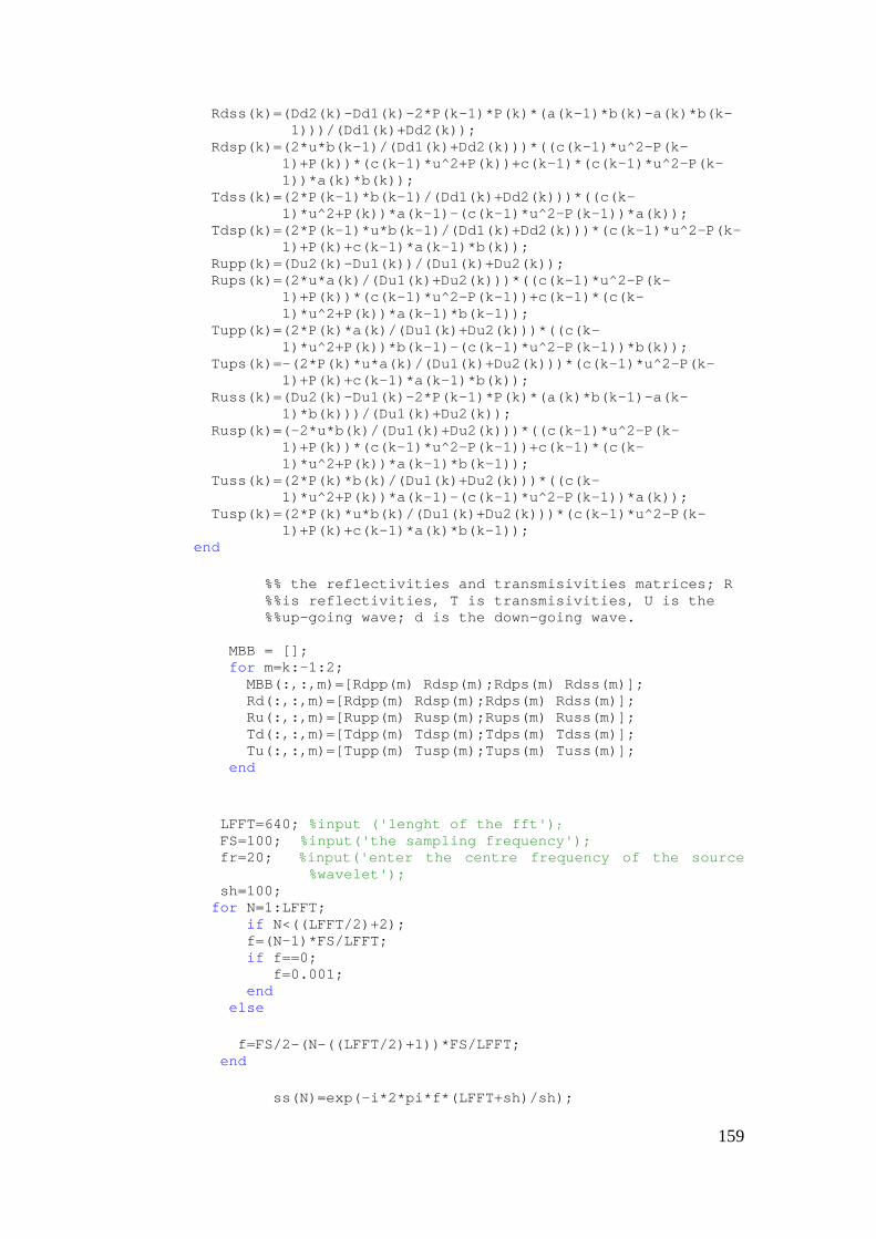
159
Rdss(k)=(Dd2(k)-Dd1(k)-2*P(k-1)*P(k)*(a(k-1)*b (k)-a(k)*b(k- 1)))/(Dd1(k)+Dd2(k)); Rdsp(k)=(2*u*b(k-1)/(Dd1(k)+Dd2(k)))*((c(k-1)* u^2-P(k- 1)+P(k))*(c(k-1)*u^2+P(k))+c(k-1)*(c(k -1)*u^2-P(k- 1))*a(k)*b(k)); Tdss(k)=(2*P(k-1)*b(k-1)/(Dd1(k)+Dd2(k)))*((c( k- 1)*u^2+P(k))*a(k-1)-(c(k-1)*u^2-P(k-1) )*a(k)); Tdsp(k)=(2*P(k-1)*u*b(k-1)/(Dd1(k)+Dd2(k)))*(c (k-1)*u^2-P(k- 1)+P(k)+c(k-1)*a(k-1)*b(k)); Rupp(k)=(Du2(k)-Du1(k))/(Du1(k)+Du2(k)); Rups(k)=(2*u*a(k)/(Du1(k)+Du2(k)))*((c(k-1)*u^ 2-P(k- 1)+P(k))*(c(k-1)*u^2-P(k-1))+c(k-1)*(c (k- 1)*u^2+P(k))*a(k-1)*b(k-1)); Tupp(k)=(2*P(k)*a(k)/(Du1(k)+Du2(k)))*((c(k- 1)*u^2+P(k))*b(k-1)-(c(k-1)*u^2-P(k-1) )*b(k)); Tups(k)=-(2*P(k)*u*a(k)/(Du1(k)+Du2(k)))*(c(k- 1)*u^2-P(k- 1)+P(k)+c(k-1)*a(k-1)*b(k)); Russ(k)=(Du2(k)-Du1(k)-2*P(k-1)*P(k)*(a(k)*b(k -1)-a(k- 1)*b(k)))/(Du1(k)+Du2(k)); Rusp(k)=(-2*u*b(k)/(Du1(k)+Du2(k)))*((c(k-1)*u ^2-P(k- 1)+P(k))*(c(k-1)*u^2-P(k-1))+c(k-1)*(c (k- 1)*u^2+P(k))*a(k-1)*b(k-1)); Tuss(k)=(2*P(k)*b(k)/(Du1(k)+Du2(k)))*((c(k- 1)*u^2+P(k))*a(k-1)-(c(k-1)*u^2-P(k-1) )*a(k)); Tusp(k)=(2*P(k)*u*b(k)/(Du1(k)+Du2(k)))*(c(k-1 )*u^2-P(k- 1)+P(k)+c(k-1)*a(k)*b(k-1)); end %% the reflectivities and transmisivitie s matrices; R %%is reflectivities, T is transmisivitie s, U is the %%up-going wave; d is the down-going wav e. MBB = []; for m=k:-1:2; MBB(:,:,m)=[Rdpp(m) Rdsp(m);Rdps(m) Rdss(m )]; Rd(:,:,m)=[Rdpp(m) Rdsp(m);Rdps(m) Rdss(m) ]; Ru(:,:,m)=[Rupp(m) Rusp(m);Rups(m) Russ(m) ]; Td(:,:,m)=[Tdpp(m) Tdsp(m);Tdps(m) Tdss(m) ]; Tu(:,:,m)=[Tupp(m) Tusp(m);Tups(m) Tuss(m) ]; end LFFT=640; %input ('lenght of the fft') ; FS=100; %input('the sampling frequency'); fr=20; %input('enter the centre frequency of the source %wavelet'); sh=100; for N=1:LFFT; if N<((LFFT/2)+2); f=(N-1)*FS/LFFT; if f==0; f=0.001; end else f=FS/2-(N-((LFFT/2)+1))*FS/LFFT; end ss(N)=exp(-i*2*pi*f*(LFFT+sh)/sh);

160
% Futterman absorption Model Vc(n-1)=V(n-1)*(1-(1/(pi*q(n-1)))*log(f/fc(n-1) ))-(i/(2*V(n- 1)*q(n-1))); % P- wave velocity Bc(n-1)=B(n-1)*(1-(1/(pi*Q(n-1)))*log(f/fc(n-1) ))-(i/(2*B(n- 1)*Q(n-1))); % S- wave velocity l2(N)=sqrt(((2*pi*f)^2/(Vc(n-1))^2)-(2*pi*f*sin d(z)/Vc(n- 1))^2); % P-wave number ll2(N)=sqrt(((2*pi*f)^2/(Bc(n-1))^2)-(2*pi*f*si nd(z)/Bc(n- 1))^2); % S- wave number E2=[exp(-i*(-l2(N))*d(n-1)) 0;0 exp(-i*(-ll2(N) )*d(n-1))];% %phase matrix for down going wave E22=[exp(i*(l2(N))*d(n-1)) 0;0 exp(i*(ll2(N))*d (n-1))];% %phase matrix for up-going waves MT=E2*Rd(:,:,k)*E22; %L is the number of layers k5= n-1; for L=k5:-1:2; A(:,:,L)=I-MT*Ru(:,:,L); BB(:,:,L)=MT*Td(:,:,L); MB(:,:,L-1)=Rd(:,:,L)+(Tu(:,:,L)*A(:,:,L)^-1 *BB(:,:,L)); Vc(L-1)=V(L-1)*(1-(1/(pi*q(L-1)))*log(f/fc(L- 1)))- (i/(2*V(L-1)*q(L-1))); Bc(L-1)=B(L-1)*(1-(1/(pi*Q(L-1)))*log(f/fc(L- 1)))- (i/(2*B(L-1)*Q(L-1))); l(N)=sqrt(((2*pi*f)^2/(Vc(L-1))^2)-(2*pi*f*si nd(z)/Vc(L- 1))^2); ll(N)=sqrt(((2*pi*f)^2/(Bc(L-1))^2)-(2*pi*f*s ind(z)/Bc(L- 1))^2); E=[exp(-i*(-l(N))*d(L-1)) 0;0 exp(-i*(-ll(N)) *d(L-1))]; EE=[exp(i*(l(N))*d(L-1)) 0;0 exp(i*(ll(N))*d( L-1))]; MT=E*MB(:,:,L-1)*EE; end MT1PP(N)=MT(1,1); end MT2PP=MT1PP.*ss; %% modeling a source impulse (e.g a Ricker w avelet) for kk=1:LFFT; if kk < (sh+1); t=-((sh+1)-kk)*1/FS; else t= (kk-(sh+1))*1/FS; end r(kk)=exp(-pi^3*fr^2/4*t^2)*(1-pi^3*fr^2/2*t^2 ); end sg=fft(r); MT2PP(1)=abs(MT2PP(1)); MT2PP(1:LFFT/2 +1)=conj(MT2PP(1:LFFT/2 +1)); MT2PP(LFFT/2 +1)=abs(MT2PP(LFFT/2 +1)); ysmtq=ifft(MT2PP.*sg); t=0:0.01:6.39; plot(t,ysmtq)
161
Appendix 2B A MATLAB code for computing inverse quality factor using the Gassmann
(1951) equation
[email protected]: modelling attenuation as a function of Saturation in partially saturated porous rock using Gassmann(1951)formulations Input: Kg=bulk modulus of Gas; Kw= bulk modulus of water; fclay=Proportion of clay in the reservoir rock ; fQfz= proportion of Quartz in the reservoir ro ck; Sw=Water saturation; Sg=Gas saturation; Kf=bulk modulus of the fluid PP=patch; P= porosity; Kdry= bulk modulus of the dry rock Gdry=shear modulus of the dry rock K=bulk modulus Numerical values of the parameters Kw=2.64; Kg=0.04;p=0.3; clay=0.05;quartz=0.95; fclay=0.05; fQtz=0.095; Kdry=2.6;Gdry=3.2; Kclay=1.45; KQtz=37.9; Mdry=Kdry+4/3*Gdry; Sw+Sg=1 for n= 1:100; Sw=n*0.01; Kf=inv(Sw/Kw +(1-Sw)/Kg); Ks=(fclay*Kclay)+(fQtz*Kclay) % atlow frequency Ksat0(n)=Ks*((p*Kdry-(1+p)*Kf*Kdry/Ks+Kf)/((1-p )*Kf+p*Ks- Kf*Kdry/Ks)); Msat0(n)= Ksat0(n)+4/3*Gdry; %at high frequency Kpp(n)=Ks*((p*Kdry-(1+p)*Kw*Kdry/Ks +Kw)/((1-p) *Kw+p*Ks- Kw*Kdry/Ks)); Ksw0(n)=Ks*((p*Kdry-(1+p)*Kg*Kdry/Ks +Kg)/((1-p )*Kg+p*Ks- Kg*Kdry/Ks)); Msat1(n)=inv( Sw/(Kpp(n)+ 4/3*Gdry) +(1-Sw)/(Ks w0(n)+ 4/3*Gdry)); �{o,�� (n)= (Msat1(n)-Msat0(n))/(2*sqrt(Msat0(n).*Msat1(n) )); end sat=1:1:100 plot(sat, ��o,�� );
162
Appendix 2C
A MATLAB code for showing the effect of irreducible water saturation on inverse quality factor, using the Gassmann (1951) equation.
% [email protected]: modelling attenuation as a %function of saturation with the consideration of i rreducible %water saturation; This code relied on appendix 2b for some %parameters %K=irreducible water saturation for n=1:100; K=40; Swir=K/100; if n<K; Sww=Swir; else Sww=n*0.01; end Fp=(Sww-Swir)/(1-Swir) % the patch saturation Kfir=inv(Swir/Kw +(1-Swir)/Kg); Kswir=Ks*((p*Kdry-(1+p)*Kfir*Kdry/Ks +Kfir)/((1-p)* Kfir+p*Ks - Kfir*Kdry/Ks)); Msat1ir(n)=inv(Fp/(Kp(n)+ 4/3*Gdry) +(1-Fp)/ (Kswir +4/3*Gdry)); if n<K; Msat0ir=Msat1ir; else Msat0ir=Msat0; �{o,�� IRR(n)=(Msat1ir(n)-Msat0ir(n))/(2*sqrt(Msat0ir(n) .*Msat1ir(n))); end end Sat=1:1:100; %saturation in percentage Plot(sat, �{o,�� IRR)
163
Appendix 2D
A MATLAB code for computing inverse quality factor using the Vp-substitution equation (Mavko et al., 1995)
[email protected]: modelling attenuation as a function of Saturation in partially saturated porous rock u sing Mavko et al.(1998)Vp–substitution equation. Input: Input: Kg=bulk modulus of Gas; Kw= bulk modulus of water; fclay=Proportion of clay in the reservoir rock ; fQfz= proportion of Quartz in the reservoir ro ck; Sw=Water saturation; Sg=Gas saturation; Kf=bulk modulus of the fluid PP=patch; P= porosity; Mclay= Compressional modulus of clay MQtz= compressional modulus of Quartz Mdry= compressional modulus of the dry rock Ms=compressional modulus of the mineral phase Given that; Kw=2.64; Kg=0.04;p=0.3; clay=0.05;quartz=0.95; Kdry=2.6;Gdry=3.2;MQtz=97;Mclay=3.28;fclay=0.05; fQtz=0.95; Mdry=Kdry+4/3*Gdry; for n= 1:100; Sw=n*0.01; Kf=inv(Sw/Kw +(1-Sw)/Kg); Ms=(fclay*Mclay)+(fQtz*MQtz); % at low frequency Msat0(n)=Ms*((p*Mdry-(1+p)*Kf*Mdry/Ms+Kf)/((1- â)*Kf+p*Ms- Kf*Mdry/Ms)); %at high frequency Mpp=Ms*((p*Mdry-(1+p)*Kw*Mdry/Ms +Kw)/((1-p)*Kw +p*Ms- Kw*Mdry/Ms)); Msw0=Ms*((p*Mdry-(1+p)*Kg*Mdry/Ms +Kg)/((1-p)*K g+p*Ms- Kg*Mdry/Ms)); Msat1(n)=inv(Sw/Mp +(1-Sw)/Msw0); �{o,�� Q(n)= (Msat1(n)-Msat0(n))/(2*sqrt(Msat0(n).*Msat1(n ))); end sat=1:1:100; %saturation in percentage plot(sat, �{o,�� )
164
Appendix 2E
A MATLAB code for showing the effect of irreducible water saturation on inverse quality factor, using Vp-substitution equation (Mavko et al., 1995)
[email protected]: Modelling attenuation as a %function of saturation with the consideration of i rreducible %water saturation; This code rely on appendix 2d fo r some %parameters. for n=1:100; K=40; Swir=K/100; if n<K; Sww=Swir; else Sww=n*0.01; end Fp=(Sww-Swir)/(1-Swir); % the patch saturation Kfir=inv(Swir/Kw +(1-Swir)/Kg); Mswir=Ms*((p*Mdry-(1+p)*Kfir*Mdry/Ms +Kfir)/((1-p)* Kfir+p*Ms- Kfir*Mdry/Ms)); Msat1ir(n)=inv(Fp/Mp +(1-Fp)/Mswir); Msat0ir(n)= Ms*((p*Mdry-(1+p)*Fp*Mdry/Ms+Fp)/((1-p) *Fp+p*Ms- Fp*Mdry/Ms)); if n<K; Msat0ir=Msat1ir; else Msat0ir=Msat0; Mdiffir(n)=Msat1ir(n)-Msat0ir(n); invQir(n)= (Msat1ir(n)-Msat0ir(n))/ (2*sqrt(Msat0ir (n) .*Msat1ir(n))); end end sat=1:1:100; %saturation in percentage plot(sat, �{o,�� IRR)
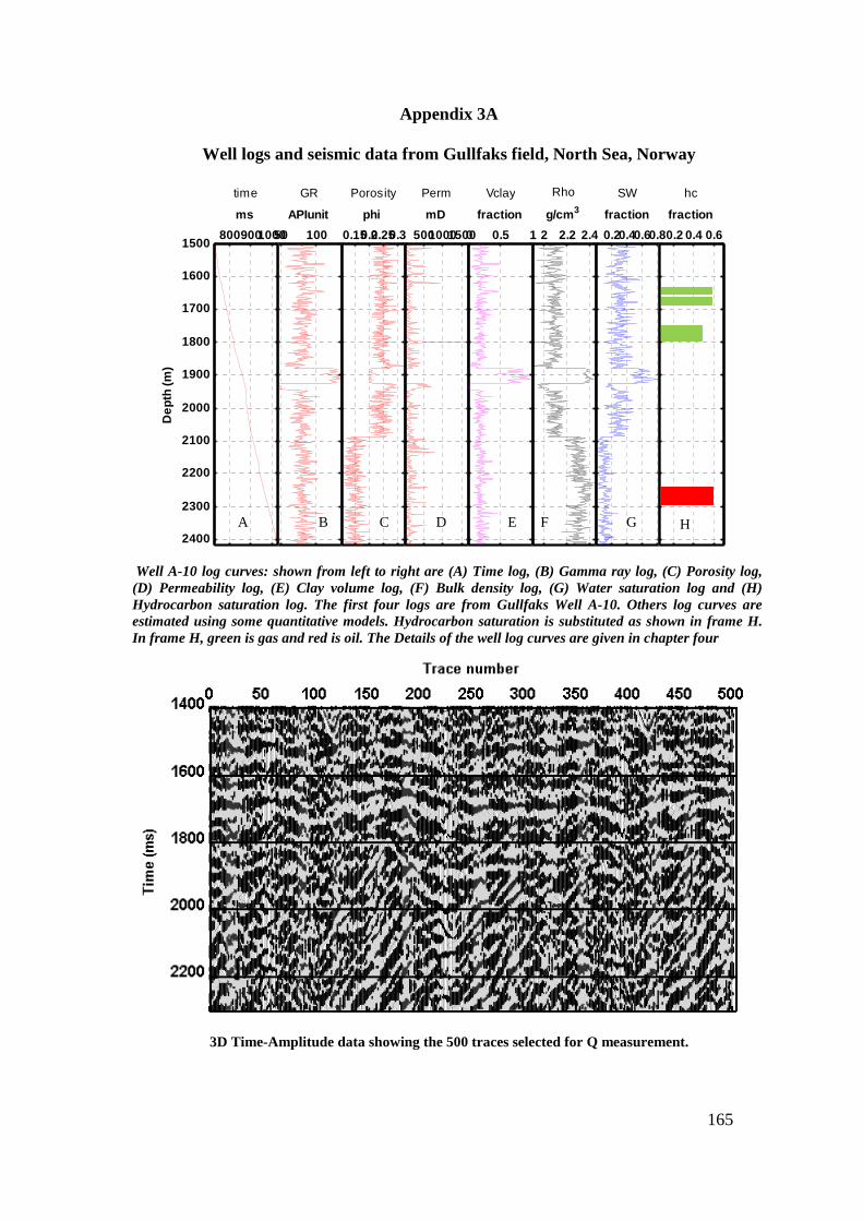
165
Appendix 3A
Well logs and seismic data from Gullfaks field, North Sea, Norway
50 100
GR
APIunit
0.150.20.250.3
Porosity
phi
50010001500
Perm
mD
0 0.5 1
Vclay
fraction
2 2.2 2.4
Rho
g/cm3
0.20.40.60.8
SW
fraction
0.2 0.4 0.6
hc
fraction
80090010001500
1600
1700
1800
1900
2000
2100
2200
2300
2400
time
ms
Dep
th (m
)
Well A-10 log curves: shown from left to right are (A) Time log, (B) Gamma ray log, (C) Porosity log, (D) Permeability log, (E) Clay volume log, (F) Bulk density log, (G) Water saturation log and (H) Hydrocarbon saturation log. The first four logs are from Gullfaks Well A-10. Others log curves are estimated using some quantitative models. Hydrocarbon saturation is substituted as shown in frame H. In frame H, green is gas and red is oil. The Details of the well log curves are given in chapter four
3D Time-Amplitude data showing the 500 traces selected for Q measurement.
A B C D E F G H

166
Appendix 3B
Work flow for Q determination in seismic records using SEISLAB interface
on MATLAB
1. Read the seismic data in to matlab using seislab interface
2. Extract the subset of the data to be analysed for Q
3. Normalise the data
4. Read the traces out one after the other
5. Determine the length of FFT and the sampled frequency from the (.traces,
step) of the field data
6. isolate/extract the wavelets that correspond to the top and the bottom of the
seismic layer to be analysed
7 record the time-location of the peak of each wavelet and compute the travel
time difference between the two wavelets
8. Do zero padding of each wavelet (according to the position on the trace) to
make up length of FFT
9. Compute the frequency spectrum of the wavelets
10. Compute centroid frequency of the wavelets
11. Compute variance and standard deviation about the centroid frequency.
12. Compute attenuation.
clear all keep WF presets Gullfaks_data=read_segy_file( 'C:\gullfaks_3D_TimeAmp.sgy' ); Sub_data=select( 'Gullfaks_data' ,{‘traces’,x,y}); Sub_data_norm=normalize(Sub_data,{‘value’,1}); % extract the wavelet of the incident signal Wavelet1a=s_select(Sub_data_norm,{‘times’, t1,t2},{ ‘traces’,1}); % extract the waveket of the transmitted signal Wavelet1b=s_select(Sub_data_norm,{‘times’, t1,t2},{ ‘traces’,1}); Define LFF; Define F; 1a= wavelet1a after zeros padding 1b= wavelet1b after zeros padding S=1a; R=1b;
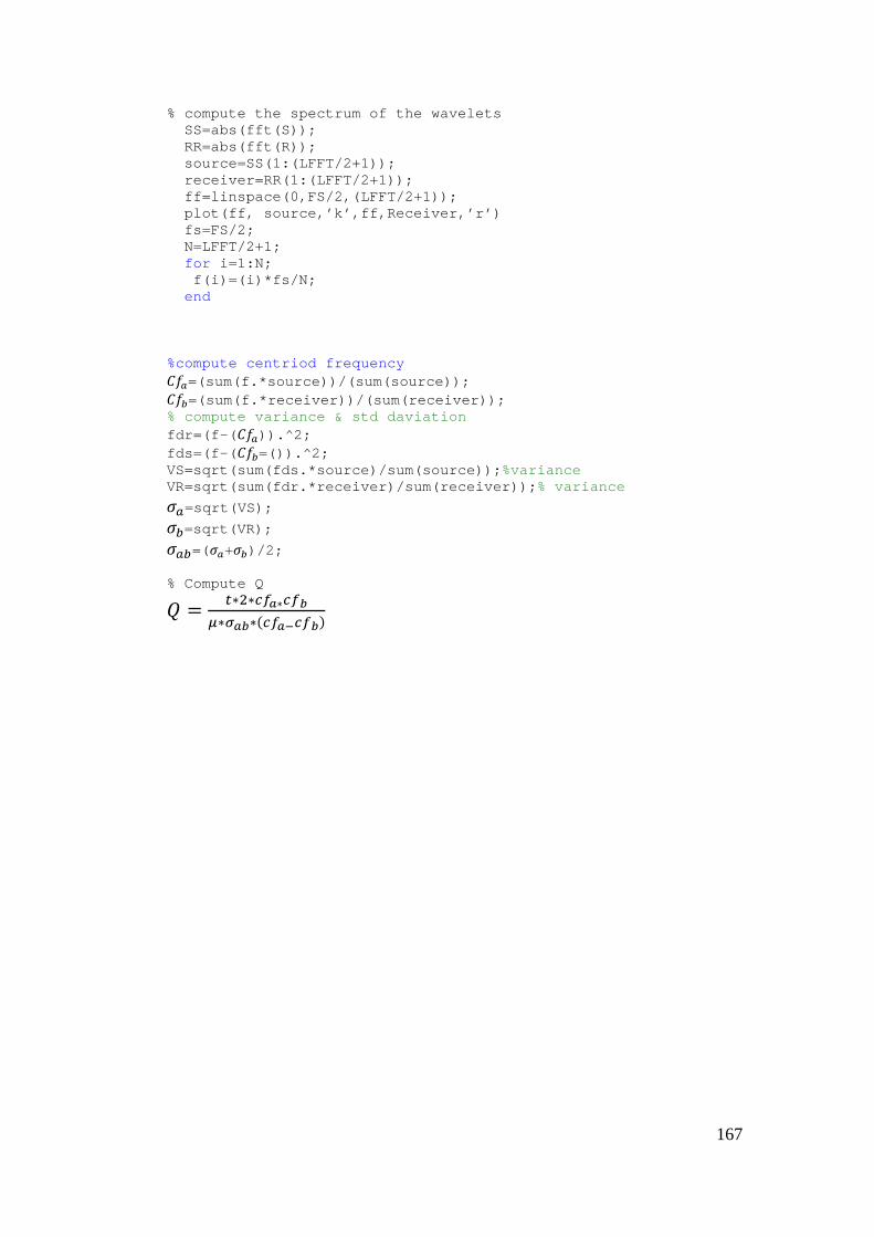
167
% compute the spectrum of the wavelets SS=abs(fft(S)); RR=abs(fft(R)); source=SS(1:(LFFT/2+1)); receiver=RR(1:(LFFT/2+1)); ff=linspace(0,FS/2,(LFFT/2+1)); plot(ff, source,’k’,ff,Receiver,’r’) fs=FS/2; N=LFFT/2+1; for i=1:N; f(i)=(i)*fs/N; end %compute centriod frequency 3o=(sum(f.*source))/(sum(source)); 3G=(sum(f.*receiver))/(sum(receiver)); % compute variance & std daviation fdr=(f-( 3o)).^2; fds=(f-( 3G=()).^2; VS=sqrt(sum(fds.*source)/sum(source)); %variance VR=sqrt(sum(fdr.*receiver)/sum(receiver)); % variance Éo=sqrt(VS); ÉG=sqrt(VR); ÉoG=( Éo+ÉG)/2; % Compute Q � Hô6ôN0�ôN0Æ�ôÈ�Æô&N0�!N0Æ�

168
-0.05 0 0.05 0.1 0.15 0.20
20
40
60
80
100
120
140
160
180
200
Appendix 3C
The Distribution of 1/Q used to compute the mean attenuation in the four intervals:
AB, BC, CD, and DE. The distribution of 1/Q³ 0 in for interval CD
0 0.01 0.02 0.03 0.04 0.05 0.060
20
40
60
80
100
120
140
160
180
200
0 0.05 0.1 0.15 0.2 0.25 0.30
20
40
60
80
100
120
140
160
180
200interval bc
-0.02 -0.01 0 0.01 0.02 0.03 0.04 0.05 0.06 0.07 0.080
50
100
150
200
250
The distribution of 1/Q³ 0 in for interval AB The distribution of 1/Q³ 0 in for interval BC
The distribution of 1/Q³ 0 in for interval CD The distribution of 1/Q³ 0 in for interval DE

169
Appendix 3D
.
4.56 4.565 4.57 4.575 4.58
x 105
6.782
6.7821
6.7822
6.7823
6.7824
6.7825
6.7826
6.7827
6.7828
6.7829
6.783
x 106
0
10
20
30
40
50
60
70
80
90
100
4.56 4.565 4.57 4.575 4.58
x 105
6.782
6.7821
6.7822
6.7823
6.7824
6.7825
6.7826
6.7827
6.7828
6.7829
6.783
x 106
0
10
20
30
40
50
60
70
80
90
100
4.56 4.565 4.57 4.575 4.58
x 105
6.782
6.7821
6.7822
6.7823
6.7824
6.7825
6.7826
6.7827
6.7828
6.7829
6.783
x 106
0
10
20
30
40
50
60
70
80
90
100
Interval AB
Q
Interval BC
Interval CD
Y C
oord
inat
e (m
) Y
Coo
rdin
ate
(m)
Y C
oord
inat
e (m
)
X coordinates (m)
X coordinates (m)
X coordinates (m) Q
Q
Maps showing Q distribution in the four intervals. The colour scale is clipped below zero

170
4.56 4.565 4.57 4.575 4.58
x 105
6.782
6.7821
6.7822
6.7823
6.7824
6.7825
6.7826
6.7827
6.7828
6.7829
6.783
x 106
10
20
30
40
50
60
70
80
90
100
Interval DE
X coordinates (m)
Y C
oord
inat
e (m
) Q

171
Appendix 3E
The layers parameters (from figure 3.14) used to generate the synthetic seismograms that is used to measure scattering attenuation.
interval Depth (m) Thickness (m) velocity m/s Density kg/m3
IJ 1500-1639 139 2210.2 2085
JK 1639-1700 61 1767.2 2102
KL 1700-1745 45 2099.9 2088
LM 1745-1800 55 1775.7 2097
MN 1800-1870 79 2139.2 2081
NP 1879-1926 47 1854.5 2352
PQ 1926-2087 161 2145.8 2087
QR 2087-225 138 2371.1 2299
RS 2225-2298 73 2586.1 2364
ST 2298-2416 118 2307.4 2297

172
Appendix 4A
Table of values for some parameter used in chapter 4
Parameter �� �� �£�Á ��oH �Ô���oM� �Ô���ãoÁ8
value 2.54 0.08 1.41 3.2 5.2 4.4
Parameter x�oH8� x£�Á x�oj x�ãoÁ8 x�oM� S
value 1.04 0.824 0.00077 2.85 2.68 4.4
Parameter ��Áo� ��Øo�Hv z�Áo� ��Áo� x�oM� ��Øo�Hv
value 1.45 37.9 95.67 3.37 2.68 44.3
Parameter xNÁo� x�Øo�Hv
value 1.58 2.65
Sources: Duffault et al.,(2011); Mavko et al., (1998) and Anderson et al., (2009) Notations and Units x represents density. The unit is in g/cm3. While � and � represents shear modulus and bulk modulus respectively. Their unit is Gpa
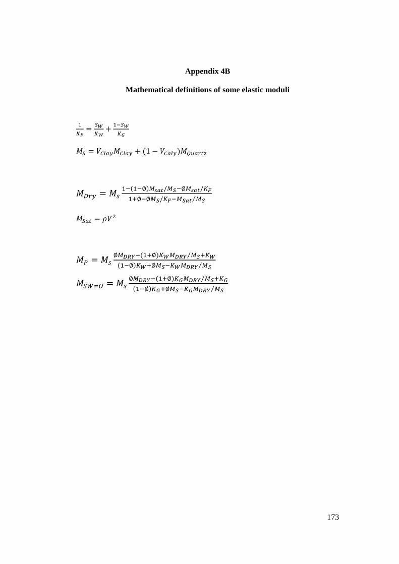
173
Appendix 4B
Mathematical definitions of some elastic moduli
��� ���� P ������
z� T�Áo�z�Áo� P &1 @ T�oÁ��z�Øo�Hv
zÔ�� zj ��&��y�{���/{#�y{���/���~y�y{#/���{#�� {#⁄
z�oH xT6
z� zj y{����&�~y���{��� {#⁄ ~��&��y���~y{#���{��� {#⁄
z���£ zj y{����&�~y���{��� {#⁄ ~��&��y���~y{#���{��� {#⁄
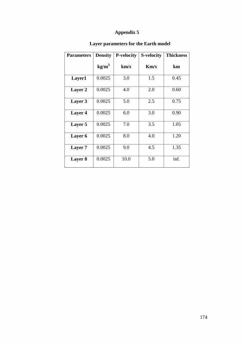
174
Appendix 5
Layer parameters for the Earth model
Parameters
Density
kg/m3
P-velocity
km/s
S-velocity
Km/s
Thickness
km
Layer1 0.0025 3.0 1.5 0.45
Layer 2 0.0025 4.0 2.0 0.60
Layer 3 0.0025 5.0 2.5 0.75
Layer 4 0.0025 6.0 3.0 0.90
Layer 5 0.0025 7.0 3.5 1.05
Layer 6 0.0025 8.0 4.0 1.20
Layer 7 0.0025 9.0 4.5 1.35
Layer 8 0.0025 10.0 5.0 inf.
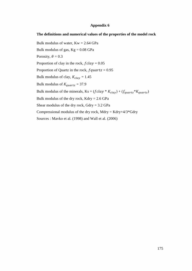
175
Appendix 6
The definitions and numerical values of the properties of the model rock
Bulk modulus of water, Kw = 2.64 GPa
Bulk modulus of gas, Kg = 0.08 GPa
Porosity, â = 0.3
Proportion of clay in the rock, 3]ni = 0.05
Proportion of Quartz in the rock, 3�Ýi�<h = 0.95
Bulk modulus of clay, �NÁo� = 1.45
Bulk modulus of � Øo�Hv = 37.9
Bulk modulus of the minerals, Ks = (3]ni * �NÁo�) + (3 Øo�Hv*� Øo�Hv)
Bulk modulus of the dry rock, Kdry = 2.6 GPa
Shear modulus of the dry rock, Gdry = 3.2 GPa
Compressional modulus of the dry rock, Mdry = Kdry+4/3*Gdry
Sources : Mavko et al. (1998) and Wall et al. (2006)