determination of seismic wave attenuation for the garhwal ... · determination of seismic wave...

Determination of Seismic Wave Attenuation for the Garhwal Himalayas, India

Soham Banerjee, Abhishek Kumar*

Department of Civil Engineering, Indian Institute of Technology Guwahati, Assam, India Email: [email protected]

Abstract. Present work determines the seismic wave attenuation characteristics in the Garhwal Himalayan, India. These are obtained based on the attenuations of P, S and coda wave spectra from the recorded seismograms of nearby earthquakes (EQs) with focal depth up to 10 km. Since P and S waves come directly to the site, attenuation of P and S waves in the present study represents the crustal attenuation characteristics of the region whereas coda wave appears from deeper lithospheric regions thus coda wave attenuation represents the attenuation characteristics of deeper lithospheric regions. Above attenuation characteristics are frequency dependent and are shown in terms of the Quality factors ( ) Q . The average −Q f correlation ( )η= oQ Q f for P, S and coda waves

obtained in the present study are ( ) ( )±± 1.065 0.048 76 9 f , ( ) ( )±± 0.927 0.099 155 36 f and

( ) ( )±± 1.059 0.036101 9 f respectively. Value of s

p

QQ

ratio greater than 1 for the study area suggests

that the crust beneath this region is composed of dry rocks. In addition, −Q f correlations for coda wave are also determined with the increasing lapse time suggesting that the upper lithosphere of Garhwal Himalayas is more heterogeneous than the lower lithosphere. The obtained −Q f correlations are essential for creating a Ground motion model in this region.

Keywords: Seismic wave attenuation, quality factor, lapse time, scale of heterogeneity.

1 Introduction

The movement of tectonic plates during an earthquake (EQ) dissipates seismic energy which spreads in the form of a spherical wavefront throughout the lithospheric medium. This seismic energy of the wave attenuates during its propagation away from the source due to geometrical spreading, intrinsic attenuation and scattering attenuation. Attenuation due to geometrical spreading does not vary with medium properties but it depends on the radius of the spherical wavefront, whereas intrinsic and scattering attenuation varies depending on the medium characteristics. Intrinsic attenuation occurs when a part of seismic energy gets converted into heat or any other form of energy depending on the elastic properties of the propagation medium. Scattering attenuation on the other hand, occurs due to redistribution of energy caused by the interaction of seismic energy with the medium heterogeneities. Thus, to characterize the lithosphere, study of seismic wave attenuation can be very helpful. Further, these attenuation characteristics of the medium are directly related to EQ generated ground motions. Hence, along with the source and site characteristics, propagation path attenuation is also an integral part of ground motion prediction models.

Attenuation characteristics of seismic wave are usually defined in terms of Quality factor ( )Q which is a frequency ( )f dependent dimensionless parameter [1]. Q represents the wave transmission quality of the medium [2] and can be expressed [3] as: ( ) η= oQ f Q f (1)

where, oQ is the value of Q at 1 Hz and η is a numerical constant. It has to be highlighted that low

oQ is associated with tectonically active areas and the value of η increases with increase in the scale of medium heterogeneity [4 and 5]. By taking logarithm, equation 1 can be represented as [3]:

Geosciences Research, Vol. 2, No. 2, May 2017 https://dx.doi.org/10.22606/gr.2017.22005 105

Copyright © 2017 Isaac Scientific Publishing GR

( ) η= +log ?oQ f logQ logf (2)

Equation 2 above represents a straight line with ologQ and η as the intercept and slope of the straight line respectively. Inverse of Q resembles seismic wave attenuation. Q values for tectonically stable regions are comparatively higher than those for tectonically active regions. These Q values are obtained considering the waveforms of different wave types, generated during EQ and recorded at a seismic recording station. Among those waves, two are primary waves (P and S) whereas others are secondary waves (surface waves, coda waves etc.). P and S waves are the compressional and shear waves respectively generated at the EQ source, whereas coda waves are backscattered waves generated from randomly distributed medium heterogeneities [6]. Determination of Q values for P, S and coda waves for various regions have been attempted by numerous researchers [3, 7, 8, 9, 10, 11, 12, 13 and 14] throughout the world.

P and S waves reach the site of interest directly from the EQ source through crustal medium whereas coda waves at a site arrive from deeper depths and also from all the directions [6]. Thus, for shallow EQs (focal depth within 70 km as per [15]), P and S wave attenuation − −（ and ）1 1

p sQ Q mostly

represents the crustal attenuation characteristics whereas attenuation of coda wave ( )−1cQ represents

the average attenuation characteristics of the deeper lithospheric regions [12]. As per [16], the spectral content of coda wave ( ),cA f t was observed to be independent of path, hypocentral distance ( )r and EQ magnitude ( )wM but decays with the increase in lapse time ( )t from the EQ origin. Lapse time

( )t here is the time elapsed after the origin of EQ. Thus, with increase in t , coda wave from the deeper part of the lithosphere appears at the seismic recording station [12]. In other words, attenuation of coda waves can determine the attenuation characteristics of deeper lithosphere.

In the present work, attenuation characteristics considering P, S and coda spectra are obtained for the Garhwal region to understand the attenuation characteristics of the upper crust and deeper lithospheric regions.

2 Methodology

The present study considers two different methodologies. One methodology focuses on determination of direct wave attenuation while second methodology talks about the determination of coda wave attenuation. These include Coda Normalization Method (CNM) to obtain direct wave attenuation and single backscattering model to obtain coda wave attenuation. Each of these methodologies is discussed in detail in following subsections.

2.1 Direct Q by CNM

In order to obtain the direct wave attenuation, CNM developed by [7] and further extended by [9] is used in this work. As the name suggests, in CNM, the coda wave spectra of the seismogram is used in order to normalize the direct wave spectra in order to obtain the direct wave attenuation. Coda wave is the backscattered wave which originates from various scattering sources when a direct wave generated during an EQ interacts with these scatterers [6]. For this reason, coda wave arrives at the tail end of the seismogram after all the direct waves pass away. As coda wave spectrum is independent of r and wM [6], thus coda spectra will be similar in various ground motion records irrespective of r and wM values of each EQ record. Direct wave spectrum on the other hand, is directly linked with r and wM values. These differences between direct and coda waves are shown in many previous studies [6 and 16]. Based on the properties of coda wave, coda normalization method was developed. [17] presented detailed literature review on CNM.

106 Geosciences Research, Vol. 2, No. 2, May 2017

GR Copyright © 2017 Isaac Scientific Publishing

[7] First developed coda normalization method to obtain S wave attenuation, which was further extended by [9] to obtain P wave attenuation. As per [9], for narrow f and wM range, the ratio of

source spectral amplitude of P and S waves ( )( )

s

p

S f

S f is a function of f which can be expressed as:

( )( )

= Constant s

p

S ff

S f (3)

Further, [9] concluded that the coda spectral amplitude ( ) ,?cA f t is proportional to both ( )sS f and

( )pS f individually as indicated by the following equation:

( ) ( ) ( )∝ ∝, ?c s pA f t S f S f (4) In addition, the coda normalized amplitude of direct P and S waves can be written as [9]:

( )( ) ( )

γπ

= − +

,Constant

,p

c p p

A f r r fln r fA f t Q f V

(5)

( )( ) ( )

γπ

= − +

,Constant

,s

c s s

A f r r fln r fA f t Q f V

(6)

where, ( ),pA f r and ( ),sA f r are the spectral amplitude of P and S waves respectively. ( )pQ f and

( )sQ f are the quality factors for P and S waves respectively. pV and sV are the average velocities of P and S waves respectively and γ is the geometrical spreading factor. Hence, γr here considers the effect of geometrical spreading in equations 5 and 6 for P and S waves respectively. It can be observed that both equations 5 and 6 are straight line equations which represent the least square regression lines for the plot of coda normalized amplitude of P and S wave versus (vs) r respectively. Thus, ( )pQ f

and ( )sQ f are obtained from the slope of the regression lines ( )π

−p p

fQ f V

and ( )π

−s s

fQ f V

respectively.

For different f ranges, the values of ( )pQ f and ( )sQ f can be obtained separately. Finally, −Q f relationships (equation 1) can be obtained from the plot of plogQ vs log f and slogQ vs log f (equation 2) for P and S waves respectively.

2.2 Coda Q ( )cQ Using Single Backscattering Model

From the work, [6] developed two models to explain the origin of coda waves. One of the models was single backscattering model where coda wave was considered as backscattered S wave, generated due to interaction of primary S wave with the medium heterogeneities. This model considered scattering to be a weak process and the effect of multiple scattering was abandoned in support of the Born approximation. As per [6], distribution of scatterers was considered uniform throughout the region. Attenuation due to geometrical spreading however was considered separately in this model. Thus, obtained cQ value from this model only represents intrinsic and scattering attenuation and not geometric attenuation. As per [6], the coda wave amplitude ( ),cA f t can be represented as a function of f and t using the equation:

( ) ( )π−

−= 1, c

ftQ

cA f t c f t e (7)

where, ( ),cA f t is root mean square (RMS) amplitude of coda wave at t from origin of the seismogram, filtered at f band with central frequency ( )cf , ( )c f is the coda source factor, −1t considers the effect of geometrical spreading for body wave and cQ is quality factor for coda wave. Taking natural logarithm, equation (7) can be expressed as:

Geosciences Research, Vol. 2, No. 2, May 2017 107


( ) ( ) π = − ,cc

fln A f t t ln c f tQ

(8)

It can be observed that equation (8) above represents a straight line equation between ( ) ,cln A f t t

and t with π−

c

fQ

and ( ) ln c f being the slope and intercept of the line respectively. In order to

obtain the values of ( ),cA f t , a coda window starting at t can be extracted from the filtered seismogram. Coda window represents coda wave spectrum which is a superposition of backscattered waves scattered from uniformly distributed scatterers throughout the region. In this work, the value of t for coda window is considered beyond twice the S wave arrival time ( )2 st to avoid the interference of S wave data with coda wave data in accordance with [6 and 18]. Values of ( ),cA f t can then be

obtained at different t from the above coda window. These calculated values of ( ) ,cln A f t t are then

plotted against corresponding t to obtain a scattered plot between ( ) ,cln A f t t and t . Least square

regression line representing equation (8) can be fit to the plotted data and cQ can be calculated from

the slope of above regression line π −

c

fQ

. Clearly, cQ can be obtained for different f and in general,

this value of cQ is observed to be increasing with f [12 and 19]. The clogQ and log f values can be plotted against each other to obtain equation 2 from which the −Q f relationship are obtained in accordance with equation 1.

As highlighted earlier, coda wave attenuation ( )−1cQ represents an average attenuation characteristic

of the region. [20] predicted that such a region can be represented by the volume of an ellipsoid whose surface projection (ellipse) can be defined as:

( ) ( ) ( )

+ =−

2 2

2 2 21

/ 2 / 2 / 2s s

x y

V t V t r (9)

where, x and y represent the locus of a point on the ellipse and sV is the S wave velocity. According to [20], two foci of this ellipse represent EQ source and recording station. Further, [20] assumed that the scatterers through which coda waves are generating, are uniformly distributed over the surface of this ellipsoid. Again in eq. (9), t represents the time taken by the wave to reach the scatterer from the EQ source plus the time taken by the wave to arrive at the recording station from the scatterer. Hence, if t increases, the volume of the ellipsoid also increases. Thus, the attenuation of coda wave determined based on longer cw represents the attenuation characteristics of deeper lithosphere. The cQ value determined from a single EQ record represents the attenuation characteristics of a region enclosed by one ellipsoid [20]. In case many EQ events are recorded at multiple stations located within a region, there will be many cQ values and thus there are chances that ellipsoids corresponding to each cQ value will overlap. In other words, if the −Q f correlation as discussed earlier, is determined considering all such cQ values, it will represent average attenuation characteristics considering the effects of all the scatterers available within that region [20].

3 Study Area

The Garhwal region considered for the present work as shown in Figure 1 lies adjacent to the western Himalayan belt. This region is near to the convergence zone of Indian plate under the Eurasian plate namely Indus Suture Zone (ISZ) which hosts many major thrusts such as, Main Central Thrust (MCT), Main Boundary Thrust (MBT) and Himalayan Frontal Thrust (HFT) along with other localized faults [12]. All these faults are active sources of EQs all along their lengths. Numerous devastating EQs which have occurred adjacent to the study area include: 1905 Kangra EQ (>7.0 wM ), 1991 Uttarkashi EQ



(6.8 wM ), 1999 Chamoli EQ (6.5 wM ) etc., which resulted in loss of lives and infrastructure. Understanding the seismic wave attenuation for the region as attempted in this work, will help in developing ground motion models as well as in understanding the attenuation characteristics of this region towards minimizing future damage scenario [21, 22, 23] as well as for seismic hazard studies [24] of important urban centers.

Figure 1. The Locations of the earthquake epicenters and recording stations are shown in blue earthquake symbols and orange home symbols respectively.

4 Ground Motions Selected

As discussed earlier, determination of regional attenuation characteristics of seismic waves require regional ground motion records. PESMOS (Program for Excellence in Strong Motion Studies) is one of the most significant database of ground motion records in India [25], maintained by Department of Earthquake Engineering, IIT Roorkee. For the present work, ground motion records at Garhwal region are taken from PESMOS database. Each of these ground motions was recorded by digital strong motion accelerographs installed in recording stations within Garhwal regions. The recording of data in accelerographs is done at a sampling rate of 200 samples per second. The data are recorded in ASCII format which were processed through computer programs to generate the baseline corrected outputs and those outputs were accessed from the PESMOS website for the present work [26].

For the present work, a total of 21 ground motions recorded during 11 EQ events in Garhwal Himalayas are considered. All the above EQ events occurred between 2005 and 2014. Epicentral locations along with the corresponding date of EQ occurrence are listed in Table 1. In addition, details of the recording stations considered in this work are shown in Table 2. All the above selected EQ events had occurred within 15 km focal depth ( )h having wM ranges from 3.0 to 5.1 and r within 100km range. Further, each of these EQ records was available in three components: one vertical and two horizontal (North-South and East-West). As per [9], P wave components are prominent in vertical



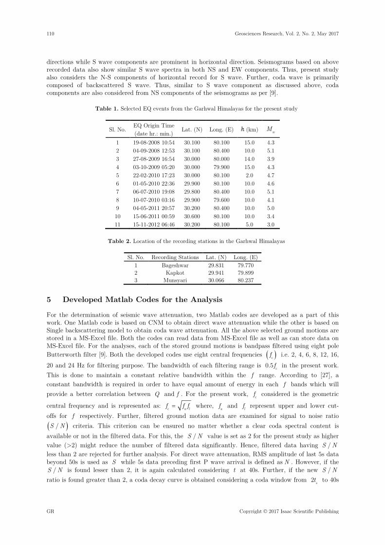
directions while S wave components are prominent in horizontal direction. Seismograms based on above recorded data also show similar S wave spectra in both NS and EW components. Thus, present study also considers the N-S components of horizontal record for S wave. Further, coda wave is primarily composed of backscattered S wave. Thus, similar to S wave component as discussed above, coda components are also considered from NS components of the seismograms as per [9].

Table 1. Selected EQ events from the Garhwal Himalayas for the present study

Sl. No. EQ Origin Time (date hr.: min.)

Lat. (N) Long. (E) (km) wM

1 19-08-2008 10:54 30.100 80.100 15.0 4.3 2 04-09-2008 12:53 30.100 80.400 10.0 5.1 3 27-08-2009 16:54 30.000 80.000 14.0 3.9 4 03-10-2009 05:20 30.000 79.900 15.0 4.3 5 22-02-2010 17:23 30.000 80.100 2.0 4.7 6 01-05-2010 22:36 29.900 80.100 10.0 4.6 7 06-07-2010 19:08 29.800 80.400 10.0 5.1 8 10-07-2010 03:16 29.900 79.600 10.0 4.1 9 04-05-2011 20:57 30.200 80.400 10.0 5.0 10 15-06-2011 00:59 30.600 80.100 10.0 3.4 11 15-11-2012 06:46 30.200 80.100 5.0 3.0

Table 2. Location of the recording stations in the Garhwal Himalayas

Sl. No. Recording Stations Lat. (N) Long. (E) 1 Bageshwar 29.831 79.770 2 Kapkot 29.941 79.899 3 Munsyari 30.066 80.237

5 Developed Matlab Codes for the Analysis

For the determination of seismic wave attenuation, two Matlab codes are developed as a part of this work. One Matlab code is based on CNM to obtain direct wave attenuation while the other is based on Single backscattering model to obtain coda wave attenuation. All the above selected ground motions are stored in a MS-Excel file. Both the codes can read data from MS-Excel file as well as can store data on MS-Excel file. For the analyses, each of the stored ground motions is bandpass filtered using eight pole Butterworth filter [9]. Both the developed codes use eight central frequencies ( )cf i.e. 2, 4, 6, 8, 12, 16, 20 and 24 Hz for filtering purpose. The bandwidth of each filtering range is 0.5 cf in the present work. This is done to maintain a constant relative bandwidth within the f range. According to [27], a constant bandwidth is required in order to have equal amount of energy in each f bands which will provide a better correlation between Q and f . For the present work, cf considered is the geometric

central frequency and is represented as: =c u lf f f where, uf and lf represent upper and lower cut-offs for f respectively. Further, filtered ground motion data are examined for signal to noise ratio ( )/S N criteria. This criterion can be ensured no matter whether a clear coda spectral content is available or not in the filtered data. For this, the /S N value is set as 2 for the present study as higher value (>2) might reduce the number of filtered data significantly. Hence, filtered data having /S N less than 2 are rejected for further analysis. For direct wave attenuation, RMS amplitude of last 5s data beyond 50s is used as S while 5s data preceding first P wave arrival is defined as N . However, if the

/S N is found lesser than 2, it is again calculated considering t at 40s. Further, if the new /S N ratio is found greater than 2, a coda decay curve is obtained considering a coda window from 2 st to 40s



and the value of ( ),cA f t at 50s is determined according to the decay curve. In coda wave attenuation, to obtain /S N , RMS amplitude of last 5s data of the coda window is used as S and 5s data preceding first P wave arrival is used as N respectively [3].

5.1 Analysis for pQ and sQ

Based on filtered seismograms obtained above, three windows surrounding the direct P wave, direct S wave and coda wave data are required to be defined to obtain pQ and sQ values. For the present analysis, the value of tw is selected as 2s. It has to be mentioned here that considering tw value greater than 2s is not possible since many of the above considered EQ events occurred near to the recording stations thus reducing the time gap between P and S wave arrival ( )Δ pst to less than 3s. [9]

studied the effects of tw on −Q f relations and found no significant change in oQ value with the increasing length of tw . It has to be highlighted there that the direct wave windows are selected from the onset of P and S wave in accordance with [9]. On a seismogram, the onset time of direct P wave ( )pt is detected visually. The S wave arrival time ( )st however cannot be visualized confidently from a

seismogram. Thus, st is determined indirectly by considering an average pV and sV values for Garhwal region as 6.5km/s and 3.6km/s respectively after [28] and using these following equations:

∆ = −

1 1ps

s p

t rV V

(10)

= + Δs p pst t t (11)

The coda window on the other hand, is selected at lapse time ( )t where, t is at the center of the coda window. This value of t has to be same for all the selected EQ records and should be greater than 2 st in order to avoid the interference of S wave data with the coda wave data [9]. Thus, for the present analysis t is considered at 50s such that most of the EQ records qualify ≥ 2 st t criteria. Once the identification of different wave records is done, peak amplitude analysis is attempted to determine ( ),pA f r and ( ),sA f r . For direct wave records, both the positive and negative peaks are determined from the above filtered P and S wave windows and the average of these two peak values are used as ( ),pA f r and ( ),sA f r respectively. For ( ),cA f t determination however, the RMS amplitudes from the filtered coda window are used referring to [9]. Above estimated values of ( ),pA f r , ( ),sA f r

and ( ),cA f t are further used to determine the values of ( )( )

γ

,

,p

c

A f r rln

A f t and

( )( )

γ

,

,s

c

A f r rln

A f t in

accordance with equations (5) and (6) respectively. Later, ( )( )

γ

,

,p

c

A f r rln

A f t and

( )( )

γ

,

,s

c

A f r rln

A f t and

are then plotted with corresponding values of r over different ranges of f as shown in Figures 2(a-h) and 3(a-h) respectively. In addition, the regression lines for each plot are also shown in Figures 2(a-h)

and 3(a-h). It has to be highlighted here that the slopes of above regression lines represent ( )π

p p

fQ f V

and ( )π

s s

fQ f V

respectively with f considered to be cf . For known values of sV , pV and f , the

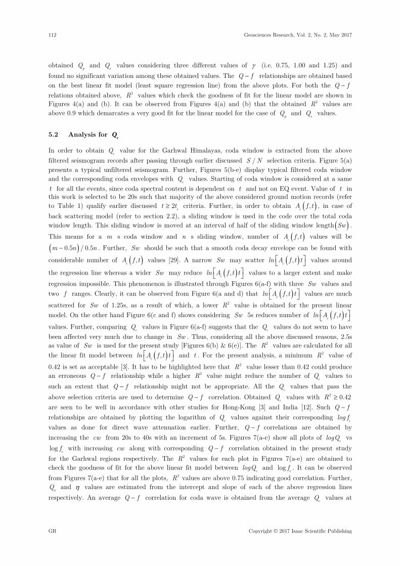
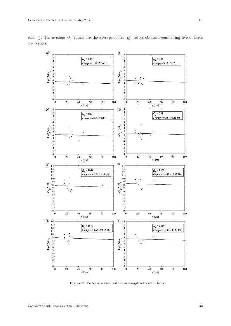
values of pQ and sQ values are obtained from those slopes corresponding to f ranges as shown in Figures 2(a-h) and 3(a-h) respectively. Further, the logarithm of above determined pQ and sQ values with the corresponding values of log cf are then plotted as shown in Figures 4(a) and (b) respectively. It has to be mentioned here that widely accepted value of 1 for γ is considered in the above analysis. [9]



obtained pQ and sQ values considering three different values of γ (i.e. 0.75, 1.00 and 1.25) and found no significant variation among these obtained values. The −Q f relationships are obtained based on the best linear fit model (least square regression line) from the above plots. For both the −Q f relations obtained above, 2R values which check the goodness of fit for the linear model are shown in Figures 4(a) and (b). It can be observed from Figures 4(a) and (b) that the obtained 2R values are above 0.9 which demarcates a very good fit for the linear model for the case of pQ and sQ values.

5.2 Analysis for cQ

In order to obtain cQ value for the Garhwal Himalayas, coda window is extracted from the above filtered seismogram records after passing through earlier discussed /S N selection criteria. Figure 5(a) presents a typical unfiltered seismogram. Further, Figures 5(b-e) display typical filtered coda window and the corresponding coda envelopes with cQ values. Starting of coda window is considered at a same t for all the events, since coda spectral content is dependent on t and not on EQ event. Value of t in this work is selected to be 20s such that majority of the above considered ground motion records (refer to Table 1) qualify earlier discussed ≥ 2 st t criteria. Further, in order to obtain ( ),cA f t , in case of back scattering model (refer to section 2.2), a sliding window is used in the code over the total coda window length. This sliding window is moved at an interval of half of the sliding window length ( )Sw . This means for a m s coda window and n s sliding window, number of ( ),cA f t values will be

( )− 0.5 / 0.5m n n . Further, Sw should be such that a smooth coda decay envelope can be found with

considerable number of ( ),cA f t values [29]. A narrow Sw may scatter ( ) ,cln A f t t values around

the regression line whereas a wider Sw may reduce ( ) ,cln A f t t values to a larger extent and make

regression impossible. This phenomenon is illustrated through Figures 6(a-f) with three Sw values and two f ranges. Clearly, it can be observed from Figure 6(a and d) that ( )

,cln A f t t values are much

scattered for Sw of 1.25s, as a result of which, a lower 2R value is obtained for the present linear model. On the other hand Figure 6(c and f) shows considering Sw 5s reduces number of ( )

,cln A f t t

values. Further, comparing cQ values in Figure 6(a-f) suggests that the cQ values do not seem to have been affected very much due to change in Sw . Thus, considering all the above discussed reasons, 2.5s as value of Sw is used for the present study [Figures 6(b) & 6(e)]. The 2R values are calculated for all the linear fit model between ( )

,cln A f t t and t . For the present analysis, a minimum 2R value of

0.42 is set as acceptable [3]. It has to be highlighted here that 2R value lesser than 0.42 could produce an erroneous −Q f relationship while a higher 2R value might reduce the number of cQ values to such an extent that −Q f relationship might not be appropriate. All the cQ values that pass the above selection criteria are used to determine −Q f correlation. Obtained cQ values with ≥2 0.42R are seen to be well in accordance with other studies for Hong-Kong [3] and India [12]. Such −Q f relationships are obtained by plotting the logarithm of cQ values against their corresponding clog f values as done for direct wave attenuation earlier. Further, − Q f correlations are obtained by increasing the cw from 20s to 40s with an increment of 5s. Figures 7(a-e) show all plots of clogQ vs log cf with increasing cw along with corresponding −Q f correlation obtained in the present study for the Garhwal regions respectively. The 2R values for each plot in Figures 7(a-e) are obtained to check the goodness of fit for the above linear fit model between clogQ and log cf . It can be observed from Figures 7(a-e) that for all the plots, 2 R values are above 0.75 indicating good correlation. Further,

oQ and η values are estimated from the intercept and slope of each of the above regression lines respectively. An average −Q f correlation for coda wave is obtained from the average cQ values at



each cf . The average cQ values are the average of five cQ values obtained considering five different cw values.

Figure 2. Decay of normalised P wave amplitudes with the r



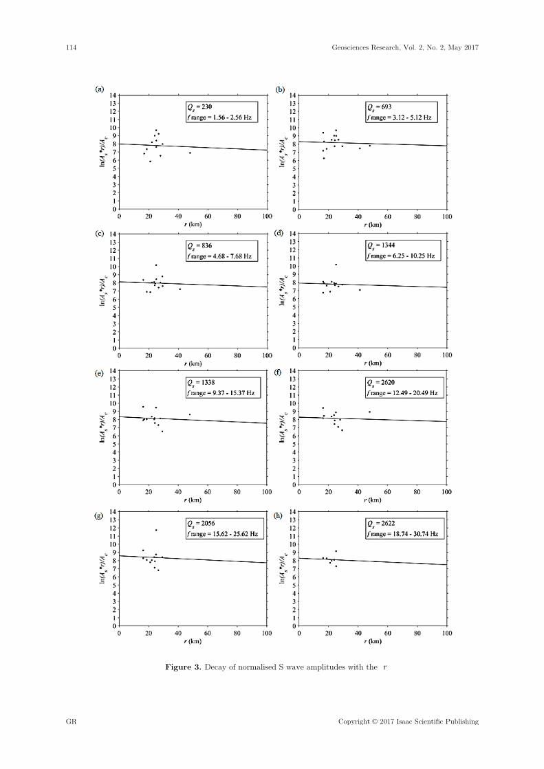
Figure 3. Decay of normalised S wave amplitudes with the r



Figure 4. −Q f correlation for P and S wave in Garhwal region

6 Results and Discussion

Above analysis for direct wave attenuation is done considering the ground motion records from the Garhwal Himalayas. Further, pQ and sQ values are obtained considering eight f ranges with 0.5 cf as bandwidth. It has to be highlighted here that the Geometrical spreading is considered separately for the present analysis. Thus, obtained pQ and sQ values show the combined effect of intrinsic and

scattering attenuation. Table 3 shows all the values of pQ , sQ and s

p

QQ

obtained from the above

analysis. Obtained values of pQ and sQ seem to increase with f which clearly indicates that the attenuation of direct wave decreases with increase in f . At low f range ( cf = 2Hz), pQ and sQ are obtained as 142 and 230 respectively as listed in Table 3. Further, for higher f range ( cf = 24 Hz), pQ

and sQ are increased to 2319 and 2622 respectively. In addition, the ratios s

p

QQ

are obtained for all the

f ranges and are found to be greater than 1 as shown in Table 3. Based on earlier studies [30, 31, 32,

33 and 34], s

p

QQ

> 1 in case crustal medium consists of dry rocks while s

p

QQ

< 1 represents a crustal



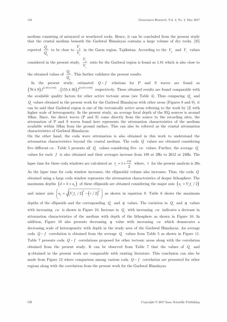
medium consisting of saturated or weathered rocks. Hence, it can be concluded from the present study that the crustal medium beneath the Garhwal Himalayas contains a large volume of dry rocks. [35]

reported s

p

QQ

to be close to p

s

VV

in the Garm region, Tajikistan. According to the pV and sV values

considered in the present study, p

s

VV

ratio for the Garhwal region is found as 1.81 which is also close to

the obtained values of s

p

QQ

. This further validates the present results.

In the present study, estimated −Q f relations for P and S waves are found as

( ) ( )±± 1.065 0.04876 9 f , ( ) ( )±± 0.927 0.099 155 36 f respectively. These obtained results are found comparable with the available quality factors for other active tectonic areas (see Table 4). Thus comparing pQ and

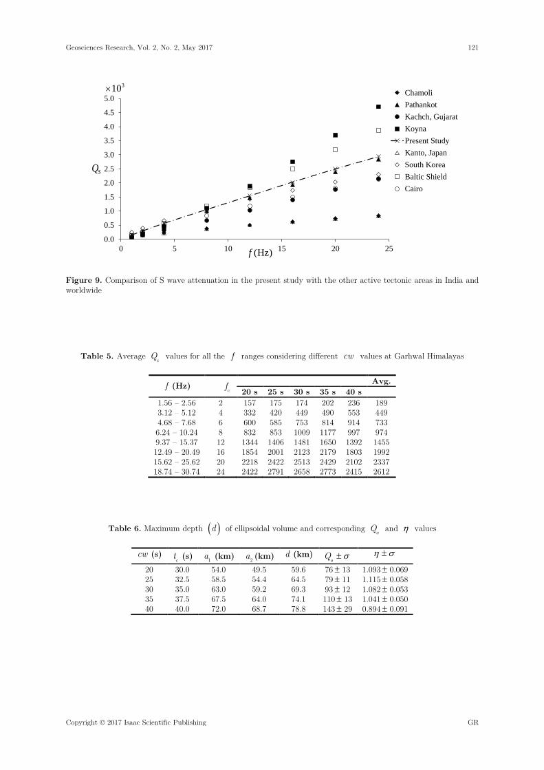
sQ values obtained in the present work for the Garhwal Himalayas with other areas (Figures 8 and 9), it can be said that Garhwal region is one of the tectonically active areas referring to the work by [3] with higher scale of heterogeneity. In the present study, an average focal depth of the EQ sources is around 10km. Since, the direct waves (P and S) come directly from the source to the recording sites, the attenuation of P and S waves found here represents the attenuation characteristics of the medium available within 10km from the ground surface. This can also be referred as the crustal attenuation characteristics of Garhwal Himalayas. On the other hand, the coda wave attenuation is also obtained in this work to understand the attenuation characteristics beyond the crustal medium. The coda Q values are obtained considering

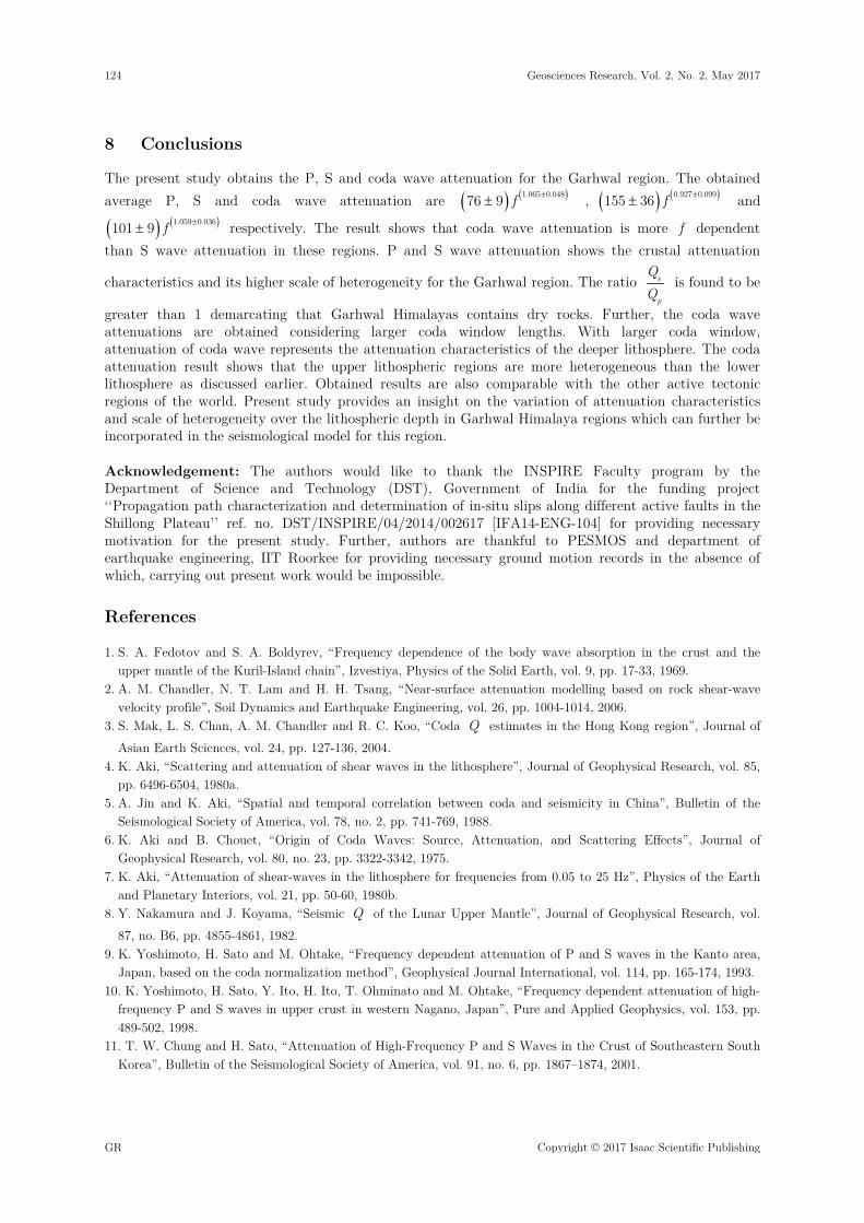
five different cw . Table 5 presents all cQ values considering five cw values. Further, the average cQ

values for each f is also obtained and their averages increase from 189 at 2Hz to 2612 at 24Hz. The

lapse time for these coda windows are calculated as = +2c

cwt t where, t for the present analysis is 20s.

As the lapse time for coda window increases, the ellipsoidal volume also increases. Thus, the coda Q obtained using a large coda window represents the attenuation characteristics of deeper lithosphere. The maximum depths ( )= + 2d h a of these ellipsoids are obtained considering the major axis ( )=1 ? / 2s ca V t

and minor axis ( ) ( ) = −

2 2

2 ? / 2 / 2s ca V t r as shown in equation 9. Table 6 shows the maximum

depths of the ellipsoids and the corresponding oQ and η values. The variation in oQ and η values

with increasing cw is shown in Figure 10. Increase in oQ with increasing cw indicates a decrease in

attenuation characteristics of the medium with depth of the lithosphere as shown in Figure 10. In addition, Figure 10 also presents decreasing η value with increasing cw which demarcates a decreasing scale of heterogeneity with depth in the study area of the Garhwal Himalayas. An average coda −Q f correlation is obtained from the average cQ values from Table 5 as shown in Figure 11.

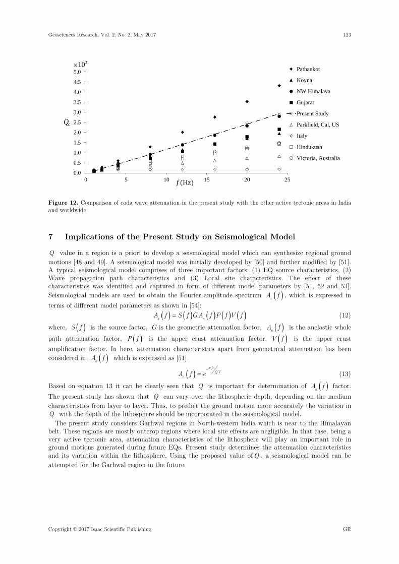
Table 7 presents coda −Q f correlations proposed for other tectonic areas along with the correlation

obtained from the present study. It can be observed from Table 7 that the values of oQ and

η obtained in the present work are comparable with existing literature. This conclusion can also be made from Figure 12 where comparison among various coda −Q f correlation are presented for other regions along with the correlation from the present work for the Garhwal Himalayas.



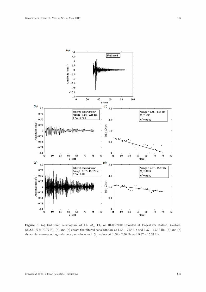
Figure 5. (a) Unfiltered seismogram of 4.6 wM EQ on 01-05-2010 recorded at Bageshwer station, Garhwal (29.831 N & 79.77 E), (b) and (c) shows the filtered coda window at 1.56 – 2.56 Hz and 9.37 – 15.37 Hz, (d) and (e) shows the corresponding coda decay envelope and cQ values at 1.56 – 2.56 Hz and 9.37 – 15.37 Hz



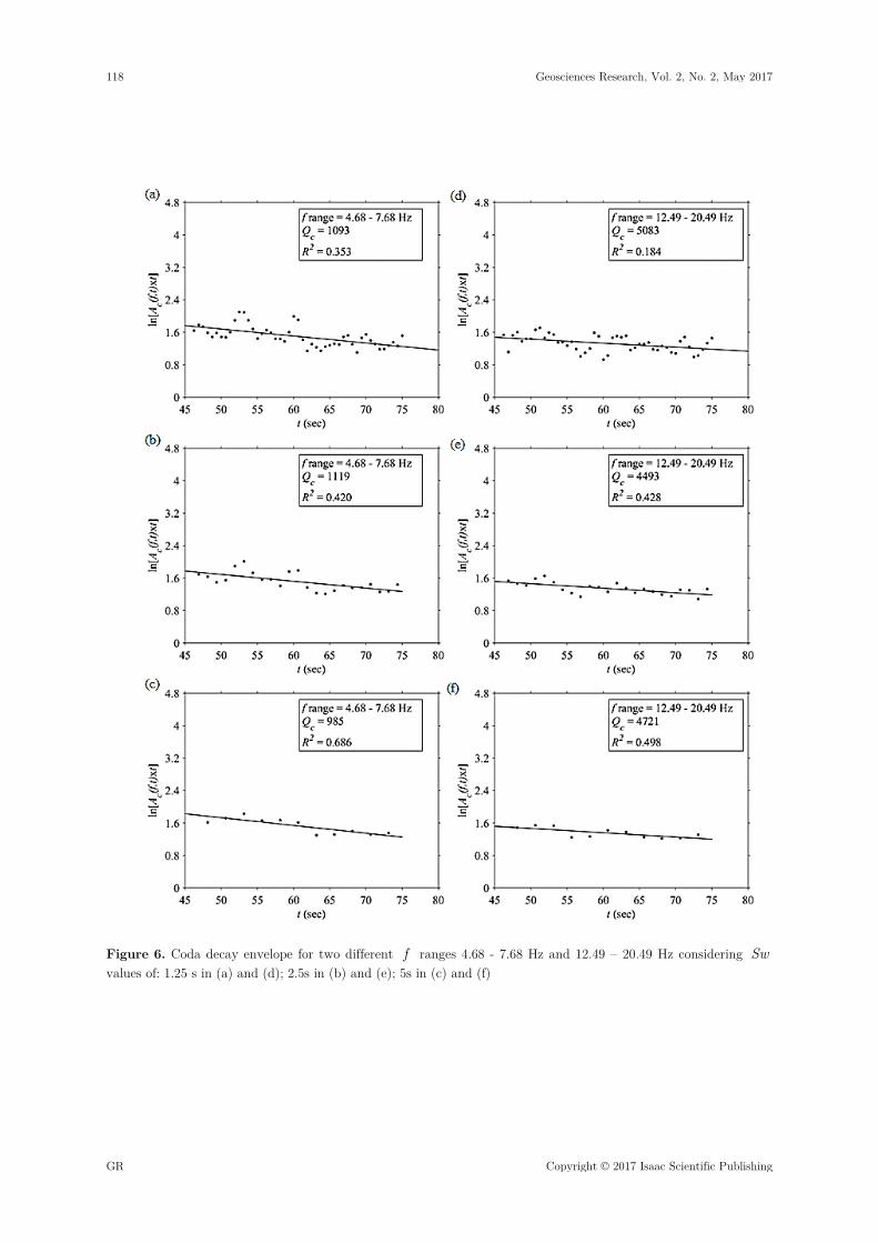
Figure 6. Coda decay envelope for two different f ranges 4.68 - 7.68 Hz and 12.49 – 20.49 Hz considering Sw values of: 1.25 s in (a) and (d); 2.5s in (b) and (e); 5s in (c) and (f)



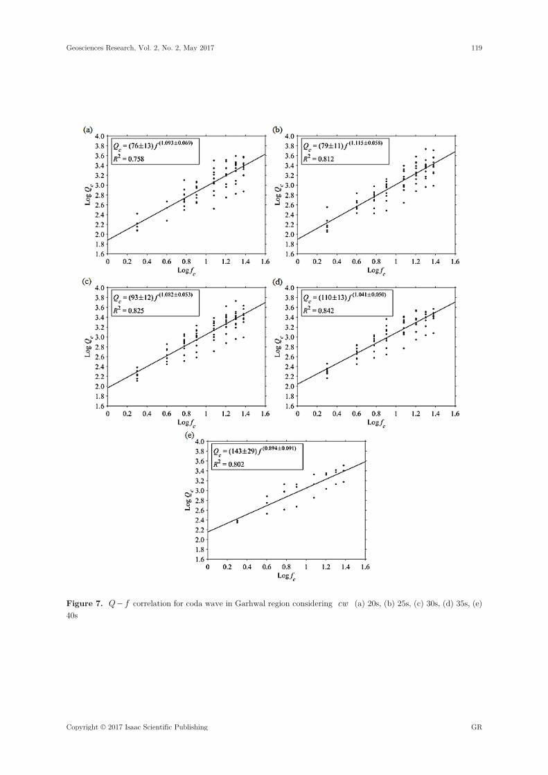
Figure 7. − Q f correlation for coda wave in Garhwal region considering cw (a) 20s, (b) 25s, (c) 30s, (d) 35s, (e) 40s



Table 3. pQ and sQ values and their ratios for all the f ranges for the Garhwal Himalayas

f (Hz) cf pQ sQ

s

p

QQ

1.56 - 2.56 2 142 230 1.624 3.12 - 5.12 4 345 693 2.008 4.68 - 7.68 6 580 836 1.443 6.25 - 10.25 8 753 1344 1.785 9.37 - 15.37 12 1094 1338 1.223 12.49 - 20.49 16 1509 2620 1.737 15.62 - 25.62 20 1542 2056 1.333 18.74 - 30.74 24 2319 2622 1.131

Table 4. Comparison of oQ and η values for P and S wave with the obtained values in other active tectonic areas in India and worldwide

Study Area P S

σ±oQ η σ± σ±oQ η σ±

Present Study 76 ± 9 1.065 ± 0.048 155 ± 36 0.927 ± 0.099 Chamoli [36] 44 ± 1 0.820 ± 0.04 87 ± 3 0.710 ± 0.03 Pathankot [19] 103 ± 8 0.990 ± 0.09 139 ± 13 0.950 ± 0.09 Kachchh, Gujarat [37] 105 0.82 74 1.06 Koyna Region [38] 59 1.04 71 1.32 Kanto, Japan [9] 32 0.95 83 0.73 South Korea [11] 111 1.05 250 0.70 Baltic Shield [39] 125 0.89 125 1.08 Cairo, Egypt [40] 53 0.80 143 0.85

0.0

0.5

1.0

1.5

2.0

2.5

3.0

3.5

0 5 10 15 20 25

ChamoliPathankotKachch, GujaratKoynaPresent StudyKanto, JapanSouth KoreaBaltic ShieldCairo

(Hz)f

pQ

310×

Figure 8. Comparison of P wave attenuation in the present study with the other active tectonic areas in India and worldwide



0.0

0.5

1.0

1.5

2.0

2.5

3.0

3.5

4.0

4.5

5.0

0 5 10 15 20 25

ChamoliPathankotKachch, GujaratKoynaPresent StudyKanto, JapanSouth KoreaBaltic ShieldCairo

(Hz)f

sQ

310×

Figure 9. Comparison of S wave attenuation in the present study with the other active tectonic areas in India and worldwide

Table 5. Average cQ values for all the f ranges considering different cw values at Garhwal Himalayas

f (Hz) cf Avg. 20 s 25 s 30 s 35 s 40 s

1.56 – 2.56 2 157 175 174 202 236 189 3.12 – 5.12 4 332 420 449 490 553 449 4.68 – 7.68 6 600 585 753 814 914 733 6.24 – 10.24 8 832 853 1009 1177 997 974 9.37 – 15.37 12 1344 1406 1481 1650 1392 1455 12.49 – 20.49 16 1854 2001 2123 2179 1803 1992 15.62 – 25.62 20 2218 2422 2513 2429 2102 2337 18.74 – 30.74 24 2422 2791 2658 2773 2415 2612

Table 6. Maximum depth ( )d of ellipsoidal volume and corresponding oQ and η values

cw (s) ct (s) 1 a (km) 2a (km) d (km) σ±oQ η σ±

20 30.0 54.0 49.5 59.6 76 ± 13 1.093 ± 0.069 25 32.5 58.5 54.4 64.5 79 ± 11 1.115 ± 0.058 30 35.0 63.0 59.2 69.3 93 ± 12 1.082 ± 0.053 35 37.5 67.5 64.0 74.1 110 ± 13 1.041 ± 0.050 40 40.0 72.0 68.7 78.8 143 ± 29 0.894 ± 0.091



Figure 10. Variation in oQ and η values with the increasing t

Figure 11. Average −Q f correlation for coda wave in the Garhwal region

Table 7. Comparison of oQ and η values for coda wave with the obtained values in other active tectonic areas in India and worldwide

Study Area Coda

σ±oQ η σ±

Present Study 101 ± 9 1.059 ± 0.036 Pathankot [12] 131 1.10 Koyna [41] 169 0.77 NW Himalayas [42] 113 1.01 Gujarat, India [43] 87 1.01 Parkfield, California [44] 79 0.74 Apenninesm Italy [45] 130 0.10 Hindukush [46] 60 1.00 Victoria, Australia [47] 100 0.85



0.0

0.5

1.0

1.5

2.0

2.5

3.0

3.5

4.0

4.5

5.0

0 5 10 15 20 25

Pathankot

Koyna

NW Himalaya

Gujarat

Present Study

Parkfield, Cal, US

Italy

Hindukush

Victoria, Australia

(Hz)f

cQ

310×

Figure 12. Comparison of coda wave attenuation in the present study with the other active tectonic areas in India and worldwide

7 Implications of the Present Study on Seismological Model

Q value in a region is a priori to develop a seismological model which can synthesize regional ground motions [48 and 49]. A seismological model was initially developed by [50] and further modified by [51]. A typical seismological model comprises of three important factors: (1) EQ source characteristics, (2) Wave propagation path characteristics and (3) Local site characteristics. The effect of these characteristics was identified and captured in form of different model parameters by [51, 52 and 53]. Seismological models are used to obtain the Fourier amplitude spectrum ( )xA f , which is expressed in terms of different model parameters as shown in [54]: ( ) ( ) ( ) ( ) ( )= x nA f S f GA f P f V f (12)

where, ( )S f is the source factor, G is the geometric attenuation factor, ( ) nA f is the anelastic whole path attenuation factor, ( ) P f is the upper crust attenuation factor, ( ) V f is the upper crust amplification factor. In here, attenuation characteristics apart from geometrical attenuation has been considered in ( ) nA f which is expressed as [51]

( )π−

= fr

QVnA f e (13)

Based on equation 13 it can be clearly seen that Q is important for determination of ( )nA f factor. The present study has shown that Q can vary over the lithospheric depth, depending on the medium characteristics from layer to layer. Thus, to predict the ground motion more accurately the variation in Q with the depth of the lithosphere should be incorporated in the seismological model.

The present study considers Garhwal regions in North-western India which is near to the Himalayan belt. These regions are mostly outcrop regions where local site effects are negligible. In that case, being a very active tectonic area, attenuation characteristics of the lithosphere will play an important role in ground motions generated during future EQs. Present study determines the attenuation characteristics and its variation within the lithosphere. Using the proposed value of Q , a seismological model can be attempted for the Garhwal region in the future.



8 Conclusions

The present study obtains the P, S and coda wave attenuation for the Garhwal region. The obtained average P, S and coda wave attenuation are ( ) ( )±± 1.065 0.04876 9 f , ( ) ( )±± 0.927 0.099 155 36 f and

( ) ( )±± 1.059 0.036101 9 f respectively. The result shows that coda wave attenuation is more f dependent than S wave attenuation in these regions. P and S wave attenuation shows the crustal attenuation

characteristics and its higher scale of heterogeneity for the Garhwal region. The ratio s

p

QQ

is found to be

greater than 1 demarcating that Garhwal Himalayas contains dry rocks. Further, the coda wave attenuations are obtained considering larger coda window lengths. With larger coda window, attenuation of coda wave represents the attenuation characteristics of the deeper lithosphere. The coda attenuation result shows that the upper lithospheric regions are more heterogeneous than the lower lithosphere as discussed earlier. Obtained results are also comparable with the other active tectonic regions of the world. Present study provides an insight on the variation of attenuation characteristics and scale of heterogeneity over the lithospheric depth in Garhwal Himalaya regions which can further be incorporated in the seismological model for this region.

Acknowledgement: The authors would like to thank the INSPIRE Faculty program by the Department of Science and Technology (DST), Government of India for the funding project ‘‘Propagation path characterization and determination of in-situ slips along different active faults in the Shillong Plateau’’ ref. no. DST/INSPIRE/04/2014/002617 [IFA14-ENG-104] for providing necessary motivation for the present study. Further, authors are thankful to PESMOS and department of earthquake engineering, IIT Roorkee for providing necessary ground motion records in the absence of which, carrying out present work would be impossible.

References

1. S. A. Fedotov and S. A. Boldyrev, “Frequency dependence of the body wave absorption in the crust and the upper mantle of the Kuril-Island chain”, Izvestiya, Physics of the Solid Earth, vol. 9, pp. 17-33, 1969.

2. A. M. Chandler, N. T. Lam and H. H. Tsang, “Near-surface attenuation modelling based on rock shear-wave velocity profile”, Soil Dynamics and Earthquake Engineering, vol. 26, pp. 1004-1014, 2006.

3. S. Mak, L. S. Chan, A. M. Chandler and R. C. Koo, “Coda Q estimates in the Hong Kong region”, Journal of Asian Earth Sciences, vol. 24, pp. 127-136, 2004.

4. K. Aki, “Scattering and attenuation of shear waves in the lithosphere”, Journal of Geophysical Research, vol. 85, pp. 6496-6504, 1980a.

5. A. Jin and K. Aki, “Spatial and temporal correlation between coda and seismicity in China”, Bulletin of the Seismological Society of America, vol. 78, no. 2, pp. 741-769, 1988.

6. K. Aki and B. Chouet, “Origin of Coda Waves: Source, Attenuation, and Scattering Effects”, Journal of Geophysical Research, vol. 80, no. 23, pp. 3322-3342, 1975.

7. K. Aki, “Attenuation of shear-waves in the lithosphere for frequencies from 0.05 to 25 Hz”, Physics of the Earth and Planetary Interiors, vol. 21, pp. 50-60, 1980b.

8. Y. Nakamura and J. Koyama, “Seismic Q of the Lunar Upper Mantle”, Journal of Geophysical Research, vol. 87, no. B6, pp. 4855-4861, 1982.

9. K. Yoshimoto, H. Sato and M. Ohtake, “Frequency dependent attenuation of P and S waves in the Kanto area, Japan, based on the coda normalization method”, Geophysical Journal International, vol. 114, pp. 165-174, 1993.

10. K. Yoshimoto, H. Sato, Y. Ito, H. Ito, T. Ohminato and M. Ohtake, “Frequency dependent attenuation of high-frequency P and S waves in upper crust in western Nagano, Japan”, Pure and Applied Geophysics, vol. 153, pp. 489-502, 1998.

11. T. W. Chung and H. Sato, “Attenuation of High-Frequency P and S Waves in the Crust of Southeastern South Korea”, Bulletin of the Seismological Society of America, vol. 91, no. 6, pp. 1867–1874, 2001.



12. N. Kumar, I. Parvez and H. Virk, “Estimation of coda wave attenuation for NW Himalayan region using local earthquakes”, Physics of the Earth and Planetary Interiors, vol. 151, pp. 243-258, 2005.

13. T. Tuve, F. Bianco, J. Ibanez, D. Patane, E. Del Pozzo, and A. Bottari, “Attenuation study in the Straits of Messina area (Southern Italy)”, Tectonophysics, vol. 421, pp. 173-185, 2006.

14. S. Baruah, D. Hazarika, N. K. Gogoi and P. S. Raju, “The effects of attenuation and site on the spectra of microearthquakes in the Jubilee Hills region of Hyderabad, India”, Journal of Earth System Science, vol. 116, no. 1, 37-47, 2007.

15. USGS, Available: https://earthquake.usgs.gov/learn/topics/determining_depth.php. 16. K. Aki, “Analysis of the Seismic Coda of Local Earthquakes as Scattered Waves”, Journal of Geophysical

Research, vol. 74, no. 2, pp. 615-631, 1969. 17. S. Banerjee and A. Kumar, “Determination of Seismic Wave Attenuation: A Review”, Disaster Advances, vol. 9,

no. 6, pp. 10-27, 2016. 18. T. G. Rautian and V. I. Khalturin, “The use of coda for determination of the earthquake source spectrum”,

Bulletin of the Seismological Society of America, vol. 68, pp. 923-948, 1978. 19. I. A. Parvez, P. Yadav and K. Nagaraj, “Attenuation of P, S and Coda Waves in the NW-Himalayas, India”,

International Journal of Geoscience, vol. 3, pp. 179-191, 2012. 20. J. J. Pulli, “Attenuation of coda waves in New England”, Bulletin of the Seismological Society of America, vol.

74, no. 4, pp. 1149-1166, 1984. 21. P. Anbazhagan, A. Kumar and T. G. Sitharam, “Site Response Deep Sites in Indo-Gangetic Plain for Different

Historic Earthquakes”, Proceedings of 5th International Conference on Recent Advances in Geotechnical Earthquake Engineering and Soil Dynamics, San Diego, California, Paper No. 3.21b: 12, San Diego, California, USA, 2010.

22. P. Anbazhagan, A. Kumar and T. G. Sitharam, “Amplification factor from intensity map and site response analysis for the soil sites during 1999 Chamoli earthquake”, 311-316, CD Proceeding of 3rd Indian Young Geotechnical Engineers Conference, New Delhi, India, 2011.

23. A. Kumar, P. Anbazhagan and T. G. Sitharam, “Site Specific Ground Response Study of Deep Indo-Gangetic Basin Using Representative Regional Ground Motions”, Proceedings of Geo-Congress2012, Oakland, California, (ASCE special Publication), 2012.

24. Kumar A, Anbazhagan P. and Sitharam T. G., “Seismic Hazard Analysis of Lucknow considering Seismic gaps”, Natural Hazards, vol. 69, pp 327-350, 2013.

25. PESMOS, Available: http://www.pesmos.in/. 26. A. Kumar, H. Mittal, R. Sachdeva and A. Kumar, “Indian Strong Motion Instrumentation Network”,

Seismological Research Letters, vol. 83, no. 1, pp. 59-66, 2012. 27. Seisan earthquake analysis software manual, Available: http://seisan.info/ 28. J. N. Tripathi, P. Singh and M. L. Sharma, “Attenuation of high-frequency P and S waves in Garhwal

Himalaya, India”, Tectonophysics, vol. 636, pp. 216-227, 2014. 29. J. M. Havskov, B. Sørensen, D. Vales, M. Özyazıcıoğlu, G. Sánchez and B. Li “Coda Q in different tectonic

areas, influence of processing parameters”, Bulletin of the Seismological Society of America, vol. 106, no. 3, pp. 1-15, 2016.

30. M. N. Toksoz, D. H. Johnston and A. Timur, (1979), “Attenuation of Seismic Waves in Dry and Saturated Rocks-I Laboratory Measurements”, Geophysics, vol. 44, no. 1, pp. 681-690, 1979.

31. D. H. Johnston, M. N. Toksoz and A. Timur, “Attenuation of Seismic Waves in Dry and Saturated Rocks: I”, Mechanics in Geophysics, vol. 44, pp. 691-711, 1979.

32. S. Mochizuki, “Attenuation in Partially Saturated Rocks”, Journal of Geophysical Research, vol. 87, no. B10, pp. 8598-8604, 1982.

33. K. W. Winkler and A. Nur, “Seismic Attenuation Effects of Pore Fluids and Frictional Sliding”, Geophysics, vol. 47, no. 1, pp. 1-15, 1982.

34. M. Vassiliou, C. A. Salvado and B. R. Tittmann, “Seismic Attenuation In CRC Hand-book of Physical Properties of Rocks (ed. Carmichael R.)”, CRC Press., Florida, 1982, pp. 295-328.

35. T. Rautian, V. Khalturin, V. Martynov and P. Molnar, “Preliminary analysis of the spectral content of P and S waves from local earthquakes in the Garm, Tadjikistan region”, Bulletin of the Seismological Society of America, vol. 68, pp. 949-971, 1978.



36. B. Sharma, S. S. Teotia, D. Kumar and P. S. Raju, “Attenuation of P and S Waves in the Chamoli Region, Himalaya, India”, Pure and Applied Geophysics, vol. 166, no. 12, pp. 1949-1966, 2009.

37. S. Chopra, B. K. Rastogi and D. Kumar, “Attenuation of High Frequency P and S Waves in the Gujarat Region, India”, Pure and Applied Geophysics, vol. 168, no. 5, pp. 797-781, 2010.

38. B. Sharma, S. S. Teotia and D. Kumar, “Attenuation of P, S and Coda Waves in Koyna Region, India”, Journal of Seismology, vol. 11, no.3, pp. 327-344, 2007.

39. L. B. Kvamme and J. Havskov, “Q in Southern Norway”, Bulletin of the Seismological Society of America, vol. 79, no. 5, pp. 1575-1588, 1989.

40. A. K. Abdel-Fattah, “Attenuation of body waves in the crust beneath the vicinity of Cairo Metropolitan area (Egypt) using coda normalization method”, Geophysical Journal International, vol. 176, pp. 126-134, 2009.

41. P. Mandal and B. K. Rastogi, “A frequency dependent relation of coda Q for Koyna-Warna Region, India”, Pure and Applied Geophysics, vol. 153, pp. 163–177, 1998.

42. S. Mukhopadhyay and C. Tyagi, “Lapse time and frequency-dependent attenuation characteristics of coda waves in the Northwestern Himalayas”, Journal of Seismology, vol. 11, pp. 149–158, 2007.

43. A. K. Gupta, A. K. Sutar, S. Chopra, S. Kumar and B. K. Rastogi, “Attenuation characteristics of coda waves in mainland Gujarat (India)”, Tectonophysics, vol. 530-531, pp. 264-271, 2012.

44. M. Hellweg, P. Spandich, J. B. Fletcher and L. M. Baker, “Stability of Coda Q in the region of Parkfield, California: view from the U.S. geological survey Parkfield dense seismograph array”, Journal of Geophysical Research, vol. 100, pp. 2089–2102, 1995.

45. L. Malagnini, R. Herrmann, and M. Di-Bona, “Ground-motion scaling in the Apennines (Italy)”, Bulletin of the Seismological Society of America, vol. 90, no. 4, pp. 1062–1081, 2000.

46. S. W. Roecker, B. Tucker, J. King and D. Hartzfeld, “Estimates of in Central Asia as a function of frequency and depth using the coda of locally recorded earthquakes”, Bulletin of the Seismological Society of America, vol. 72, pp. 129–149, 1982.

47. J. Wilkie and G. Gibson, “Estimation of seismic quality factor ( )Q for Victoria, Australia”, AGSO journal of

Australian Geology and Geophysics, vol. 15, no. 4, pp. 511–517, 1995. 48. P. Anbazhagan, A. Kumar and T. G. Sitharam, “Ground Motion Predictive Equation Based on recorded and

Simulated Ground Motion Database”, Soil Dynamics and Earthquake Engineering, vol. 53, pp 92-108, 2013. 49. A. Kumar, “Seismic microzonation of Lucknow based on region specific GMPE’s and geotechnical field studies”,

PhD Thesis, Indian Institute of Science, Bangalore, India, 2013. 50. J. N. Brune, “Tectonic stress and the spectra of seismic shear waves from earthquakes”, Journal of Geophysical

Research, vol. 75, pp. 4997-5009, 1970. 51. D. M. Boore and G. Atkinson, “Stochastic prediction of ground motion and spectral response parameters at

hard-rock sites in eastern north America”, Bulletin of the Seismological Society of America, vol. 73, pp. 1865-1894, 1987.

52. D. M. Boore, “Stochastic simulation of high frequency ground motions based on seismological model of the radiated spectra”, Bulletin of the Seismological Society of America, vol. 73, no. 6, pp. 1865-1894, 1983.

53. T. C. Hanks and R. K. McGuire, “The character of high-frequency strong ground motion”, Bulletin of the Seismological Society of America, vol. 71, no. 6, pp. 2071-2095, 1981.

54. N. T. Lam, J. Wilson and G. Hutchinson, “Generation of synthetic earthquake accelerograms using seismological modelling: A Review”, Journal of Earthquake Engineering, vol. 4, no. 3, pp. 321-354, 2000.



determination of seismic wave attenuation for the garhwal ... · determination of seismic wave...

Documents