Seismic attenuation from recordings of ambient noise

Cornelis Weemstra1, Lapo Boschi2, Alexander Goertz3, and Brad Artman4

ABSTRACT

We applied seismic interferometry to data from an ocean-bottom survey offshore Norway and found that ambient seis-mic noise can be used to constrain subsurface attenuation ona reservoir scale. By crosscorrelating only a few days ofrecordings by broadband ocean bottom seismometers, wewere able to retrieve empirical Green’s functions associatedwith surface waves in the frequency range between 0.2 and0.6 Hz and acoustic waves traveling through the sea waterbetween 1.0 and 2.5 Hz. We discovered that the decay ofthese surface waves cannot be explained by geometricalspreading alone and required an additional loss of energywith distance. We quantified this observed attenuation inthe frequency domain using a modified Bessel function todescribe the cross-spectrum in a stationary field. We aver-aged cross-spectra of equally spaced station couples andsorted these azimuthally averaged cross-spectra with dis-tance. We then obtained frequency-dependent estimates ofattenuation by minimizing the misfit of the real parts to adamped Bessel function. The resulting quality factors asfunction of frequency are indicative of the depth variationof attenuation and correlated with the geology in the surveyarea.

INTRODUCTION

Passive seismic interferometry involves the crosscorrelation ofambient seismic noise recordings. The idea stems from the deriva-tion of Claerbout (1968), who shows that the autocorrelation of thetransmission response of a seismic noise source in the subsurfacebelow a horizontally layered medium yields the reflection response

of these horizontal reflectors plus its time-reversed version. He latermade an analogous conjecture for the 3D earth (Rickett and Claerb-out, 1999). In the 1980s and 1990s, several attempts have beenmade to retrieve this impulse response from crosscorrelation of realdata, with the first convincing proof of concept produced by solarseismology (Duvall et al., 1993). The first successful application toacoustics, including a detailed proof of the theory, can be attributedto Lobkis and Weaver (2001). Other theoretical derivations aregiven, e.g., by Derode et al. (2003) and Snieder (2004) and, usinga reciprocity theorem, by Wapenaar (2004). The first successful ap-plication to the solid earth is due to Campillo and Paul (2003), whouse seismic coda.Shapiro and Campillo (2004) build on the work of Campillo and

Paul (2003), showing that broadband Rayleigh waves emerge notonly from the coda of earthquakes, but also by crosscorrelating am-bient seismic noise recordings. These surface waves can be used forvelocity inversion on a continental scale (Shapiro et al., 2005; Yanget al., 2007) as well as on a local scale (Brenguier et al., 2007;Bussat and Kugler, 2009). An elegant derivation of the underlyinginterferometric theory for surface waves is given by Tsai (2009). Ithas been shown that under certain circumstances and for specificlocations and bandwidths, body waves can also be retrieved fromthe ambient seismic wavefield (e.g., Roux et al., 2005; Draganovet al., 2007; Zhang et al., 2009; Goertz et al., 2012; Poli et al.,2012).Ambient noise sources strongly vary with location and frequency.

High levels of seismic noise are observed worldwide in the fre-quency band from 0.05 to about 1 Hz (Peterson, 1993). The mainpeak within this bandwidth is the microseism peak. Microseismsare caused by ocean wave energy coupling into the solid earth.Typically, two types of microseisms, dubbed “primary” and “second-ary,” are observed at seismic stations. While the primary (or “single-frequency”) microseisms have the same frequency as the oceanwaves that generate them, i.e., !0.08 Hz, secondary (or “double-frequency”) microseisms are observed at twice this frequency.

Manuscript received by the Editor 16 April 2012; revised manuscript received 22 July 2012; published online 11 December 2012.1Spectraseis, Inc., Denver, Colorado, USA; ETH Zürich, Institute of Geophysics, Zürich, Switzerland. E-mail: kweemstra@gmail.com.2UPMC, Université Paris, CNRS, Institut des Sciences de la Terre de Paris, Paris, France; University of Zürich, Institute of Theoretical Physics, Zürich,

Switzerland. E-mail: boschi@tomo.ig.erdw.ethz.ch.3Presently PGS Geophysical AS, Lysaker, Norway; formerly ETH Zürich, Swiss Seismological Service, Zürich, Switzerland. E-mail: alexander.goertz@

gmail.com.4Spectraseis, Inc., Denver, Colorado, USA. E-mail: brad.artman@spectraseis.com.

© 2012 Society of Exploration Geophysicists. All rights reserved.

Q1

GEOPHYSICS, VOL. 78, NO. 1 (JANUARY-FEBRUARY 2013); P. Q1–Q14, 14 FIGS.10.1190/GEO2012-0132.1

Dow

nloa

ded

12/1

3/12

to 1

92.3

3.10

4.10

4. R

edist

ribut

ion

subj

ect t

o SE

G li

cens

e or

cop

yrig

ht; s

ee T

erm

s of U

se a

t http

://lib

rary

.seg.

org/

Explanations for the origin of microseisms were first given byLonguet-Higgins (1950) and Hasselmann (1963), but see, e.g.,Stehly et al. (2006), Yang and Ritzwoller (2008), and Landéset al. (2010) for an updated discussion.Recently, several researchers focus on estimating attenuation

based on interferometric measurements of surface-wave empiricalGreen’s functions (EGFs) made on regional-scale (!100–1000 km)seismic arrays (Prieto et al., 2009; Lawrence and Prieto, 2011;Lin et al., 2011). We show here that the methodologies developedin those studies can be applied equally well at the local(!10–100 km) scale. Robust estimates of seismic attenuation at thissmall scale are needed for several reasons. First, surface waves tra-veling through sedimentary basins, whose seismic velocity is low,are amplified by virtue of energy conservation, but the low-qualityfactor that also characterizes sediments counters this effect, redu-cing amplitudes again. Neglecting this phenomenon may lead tooverestimation of ground-motion predictions. Second, hydrocarbonreservoirs exhibit an abnormally strong attenuation contrast (Chap-man et al., 2006), and measuring attenuation based on the observedambient seismic wavefield might thus help us to discriminate areservoir’s fluid content. It should be noted that, as a consequence,the inversion of the ambient seismic wavefield for attenuation mayprovide a means to image hydrocarbon reservoirs. Finally, a goodS-wave velocity and attenuation model of the shallow subsurfacewould help to improve S-wave static corrections needed in oiland gas exploration.Prieto et al. (2009) show how 1D depth profiles of phase velocity

and quality factor can be effectively derived from stacked crosscor-relations of ambient noise. This approach is extended to the case of3D velocity/quality factor heterogeneity by Lawrence and Prieto(2011), who recover phase velocity and attenuation coefficientmaps at periods of 8–32 s for the western United States. Lin et al.(2011) follow a different approach, evaluating amplitude-decay oftime-domain crosscorrelations.We adapt the approaches of Prieto et al. (2009) and Lin et al.

(2011) to the reservoir-scale inverse problem associated with seis-mic recordings collected by a broadband ocean-bottom survey inthe North Sea, covering an area of !220 km2 and with averageinterstation spacing of !500 m. This demands several changes,described below, to the data preprocessing and inversion proceduresof Prieto et al. (2009) and Lin et al. (2011). We do not invert forvelocity and attenuation structure as a function of depth, but merelycompare the frequency-dependent velocity and attenuation to thedepth-dependent geology, finding an interesting correlation.We first identify an amplitude decay of the EGFs that cannot be

associated with geometrical spreading and hence represents theeffect of energy dissipation and scattering. Second, we provide areliable estimate of this excess decay in the study area based onthe frequency-domain results of our experiment. Because of theshort duration of the survey, and the difficulties intrinsic to operat-ing ocean-bottom instrumentation, however, available data do notallow to robustly constrain lateral variations in attenuation.In the following, we first summarize the theory of seismic noise

interferometry and its relation to the normalized spatial autocorrela-tion (SPAC) of Aki (1957). We point out the necessary assumptionsand approximations and consequent limitations of our formulation.We then describe the database available to us, formulate theassociated inverse problem, and finally discuss its solution andimplications.

THEORY

An isotropic wavefield is a prerequisite for obtaining symmetricEGFs (Snieder et al., 2007). Such a wavefield can be generated bya homogeneous distribution of uncorrelated stochastic sources sur-rounding the array (e.g., Larose et al., 2006; Wapenaar et al., 2010),or by multiple scattering among heterogeneities in a complex med-ium (Campillo and Paul, 2003). The relation between the SPACapplied to a seismic wavefield (Aki, 1957) on one hand andtime-domain crosscorrelation of ambient seismic noise on the otherhand, pointed out by Yokoi and Margaryan (2008) and shown ex-plicitly by Tsai andMoschetti (2010), is the backbone of the methodapplied here because it justifies azimuthal averaging of crosscorre-lations in a nonisotropic seismic wavefield.Given the recordings u!x1" and u!x2", captured at surface loca-

tions x1 and x2, the normalized time-domain crosscorrelation Cx1x2is defined as

Cx1x2!t" "1

2T

ZT

#Tu!x1; !"u!x2; ! # t"d!; (1)

where t is time, ! is integration time, and correlation time is givenby 2T.In general, the SPAC is used to find similarities in a spatial field

by evaluating, for different space shifts !, the product of the fieldwith a space-shifted version of itself. This product is then integratedover, and normalized by the size of the field A, where the unit of Adepends on the dimension of the actual field, e.g., m2 for area orm3 for volume. The SPAC, as applied by Aki, similarly yields the“coherency” "!!" of a time-dependent wavefield u!x; t" for a shiftin space by ! and is defined as

"!!; t" " 1

A

Z

Au!x; t"u!x# !; t"dx; (2)

where x denotes position and A describes the area over which thewavefield is evaluated. The integration over, and normalization by Ain equation 2 averages the product in the integral over different x.For that reason, "!!" is also called the spatially averaged coherency(Asten, 2006).Aki (1957) assumes a wavefield that is stationary in time and

space. Here, “stationary” means that the amplitude is describedby a stochast, whose joint probability distribution does not changewhen shifted in time or space. It follows that for such a wavefield,the integral in equation 2 can be replaced by a time integral (Aki,1957):

"!!" " 1

2T

ZT

#Tu!x; t"u!x# !; t"dt: (3)

An important requirement here is that T needs to be sufficientlylong to obtain an approximately constant "!!". The assumptionof a stationary u!x; t", makes "!!" independent of x.Following Aki (1957), an “average coherency” h"i can be

introduced,

h"!r"i " 1

2#

Z

j$j$r"!!"d! $ 1

2#

Z2#

0"!j!j $ r"d%; (4)

with j!j $ r being the distance between two stations and % beingtheir azimuth. After replacing "!!" in equation 4 with its expres-sion 3, we obtain

Q2 Weemstra et al.

Dow

nloa

ded

12/1

3/12

to 1

92.3

3.10

4.10

4. R

edist

ribut

ion

subj

ect t

o SE

G li

cens

e or

cop

yrig

ht; s

ee T

erm

s of U

se a

t http

://lib

rary

.seg.

org/

h"!r $ j!j"i " 1

4#T

Z2#

0

ZT

#Tu!x; t"u!x# !; t"dtd%: (5)

It is important to note here that the average coherency is an averageover time and azimuth, while the coherency is only an average overtime (see equation 3.) The averaging is completely transparent in theideal case of noise sources distributed uniformly in azimuth: in thiscase, "!!" $ h"!r"i if j!j $ r.Tsai and Moschetti (2010) consider a single deterministic

wave of frequency & and solve the time integral in equation 3assuming the correlation time 2T is sufficiently long with respectto the period of the waves. They next combine (through a simpleintegral) multiple sources, assuming them to be uncorrelated suchthat the crosscorrelations of signals generated by different sources(the “cross-terms”) cancel out. This assumption is equivalentto the assumption of stationarity by Aki (1957). Similar assump-tions have been made by other authors (Lobkis and Weaver,2001; Snieder, 2004; Wapenaar, 2004). Through this procedure,Tsai and Moschetti (2010) find analytically that

h"!r;&"i"!0;&"

$ J0

!r&c!&"

"; (6)

where J0 denotes the zeroth-order Bessel function of the first kindand c!&" is the wave velocity as a function of angular frequency.This expression coincides with equation (42) of Aki (1957). Theleft-hand side of equation 6 is denoted h'!r;&"i " h"!r;&"i$"!0;&" and dubbed the “averaged complex coherency.” Note thatthis averaged complex coherency is normalized by the energy("!0;&"), which will be independent of location and frequencyfor a stationary wavefield.Tsai and Moschetti (2010) also show that the real part of the

crosscorrelation spectrum coincides with the SPAC. If we definethe cross-spectrum Cx1x2 !&" " F%Cx1x2!t"&, where F is the Fourier-transform operator, we get

!%Cx1x2!&"& $ "!!;&": (7)

The operator !%:::& maps its complex argument into its real part,! $ x1 # x2. For a stationary wavefield, this crosscorrelation spec-trum, similar to the SPAC in equation 3, will converge toward onevalue when averaged over time. Equation 7, together with equa-tion 6, implies that an isotropic source distribution results in!%Cx1x2!&"& coinciding with J0!j!j&$c!&"" multiplied by a con-stant related to the power at frequency &, while its imaginary partwill be zero (Tsai and Moschetti, 2010).Time-averaging of coherencies stabilizes the average coherency

in the case of a stationary wavefield (Okada, 2003). We denoteE%Cx1x2!&"& the ensemble average of Cx1x2!&" over different timewindows. Similar to the normalization of the average coherencyby the time-averaged energy "!0;&" to obtain the averaged complexcoherency h'!r;&"i, we can normalize E%Cx1x2!&"& with respectto the time-averaged power of the wavefield at the two stationsat x1 and x2, which is approximated by

##########################################ju!x1;&"j2ju!x2;&"j2

p.

If the source distribution is anisotropic, one can average both sidesof equation 7 over azimuth and using equation 6 we get

$!fE%Cx1x2!&"&g#####################################################

E%ju!x1;&"j2&E%ju!x2;&"j2&p

%$ h'!r;&"i

$ J0

!r&c!&"

": (8)

Azimuthal averaging is, just as for Aki’s SPAC, over all x1 and x2for which jx1 # x2j $ r.If the source distribution changes sufficiently over a certain time

span, averaging over this time span is similar to averaging overazimuth for a fixed source distribution (Chávez-García et al.,2005). This means that if one has data for a “sufficient” amountof time, one can set up an inverse problem for a single stationcouple, i.e., fixed !, with the phase-velocity dispersion c!&" as un-known. Ekström et al. (2009) implement such an inverse problemby equating the known zeros of J0!j!j&$c!&"" to the observed zerocrossings of !%Cx1x2!&"&.It should be noted that throughout this formulation, azimuthal

averaging would not be needed in the ideal case of a wavefield gen-erated by an azimuthally uniform distribution of sources. In the realworld, averaging is needed to mimic an isotropic wavefield, com-bining a random set of ballistic fields recorded at different timesand/or locations.The way of calculating the averaged complex coherency in equa-

tion 8 is the de facto standard practice in the SPAC community(Okada, 2003), that is, the cross-spectra are first ensemble averagedand subsequently normalized by the average power spectra (Okada,2003). Tsai (2011, equation 21) evaluates essentially the same ex-pression, deriving the coherency in the limit of infinite time forfixed sources with random phases, and hence assuming a stationarywavefield. In the case of Tsai (2011), this assumption is requiredto justify neglecting the aforementioned cross-terms. While thisassumption is theoretically correct, it is somewhat unrealistic inthe application to real seismic data as these are, in general, recordedover a wavefield that is subject to continuous change (see, e.g.,Stehly et al., 2006; Olofsson, 2010). A recent theoretical derivationbased on the SPAC formulation shows how the averaged complexcoherency behaves in dissipative media (Nakahara, 2012).Recent successful studies using surface waves obtained from am-

bient noise to constrain subsurface attenuation use a modified ex-pression of equation 8 (Prieto et al., 2009; Lawrence and Prieto,2011). The latter authors “whiten” the recordings prior to crosscor-relation and obtain the “whitened complex coherency”

(!r;&" "$E&

!%Cx1x2!&"&ju!x1;&"jju!x2;&"j

'%: (9)

Whitening is a commonly used tool to increase signal-to-noiseratios of signal from crosscorrelations of ambient seismic noise(Bensen et al., 2007; Brenguier et al., 2007; Seats et al., 2012).Whitened spectra are relieved of contamination by resonance peaksin the spectra (Bensen et al., 2007; Brenguier et al., 2007) and allowfor the wavefield to be nonstationary between individual time win-dows. The whitened complex coherency will be a scaled version ofthe Bessel function

(!r;&" $ A!&"J0!

r&c!&"

": (10)

Attenuation from ambient noise Q3

Dow

nloa

ded

12/1

3/12

to 1

92.3

3.10

4.10

4. R

edist

ribut

ion

subj

ect t

o SE

G li

cens

e or

cop

yrig

ht; s

ee T

erm

s of U

se a

t http

://lib

rary

.seg.

org/

The proportionality factor A!&", with a value between 0 and 1,needs to be introduced to account for the cross-terms and is dueto the difference in normalization between equations 8 and 9.The two amplitudes in the denominator of equation 9, i.e.,ju!x1;&"j and ju!x2;&"j, are not individually ensemble averagedand hence have a high probability of being different valued fordifferent time windows. This is due to the random phase of thecross-terms (Tsai, 2011, equation 18). Conversely, the two ensem-ble-averaged amplitudes in the denominator of equation 8 will beclose to equal valued. This important consideration could poten-tially be used to obtain an ideal period of time over which to applyequation 8 after which expression 9 could be used to average overthese periods; this is beyond the scope of this work, however. Weacquiesce in using equations 9 and 10 in the knowledge that eachinterstation distance is equally affected by this phenomenon; i.e.,A!&" is independent of r.Equation 10 clearly does not account for the effects of attenua-

tion. Prieto et al. (2009) propose to include attenuation through mul-tiplication by an exponential factor e#)!&"r,

(!r;&" $ A!&"J0!

r&c!&"

"e#)!&"r: (11)

The “attenuation coefficient” )!&" accommodates a more rapiddecrease of the Bessel function with interstation distance r, repre-senting the effect of energy dissipation and scattering. The ) isrelated to the surface wave quality factor Q by (Aki and Richards,2002)

)!&" $!

&2QU!&"

"; (12)

where U!&" is the group velocity. Given a series of azimuthally andtemporally averaged complex coherencies for various interstationdistances, a frequency-dependent estimate of Q can be obtained.As surface waves of different frequencies sample different depths,the change of Q with frequency can, to the first order, be associatedwith a change in material properties as a function of depth. Thefrequency-dependent estimate of Q is obtained by minimizingthe error on the fit of the “damped” Bessel function to the real partsof the averaged complex coherencies.Tsai (2011) shows that in the presence of attenuation, the source

distribution determines how the coherency decays with distance. Heshows for a number of specific source distributions how the real partof the coherency behaves as a function of distance for a laterallyinvariant c!&" and )!&". If one evaluates the decay of the (azimuth-ally) averaged complex coherency, however, only radial symmetricsource distributions need to be considered, and the behavior of thecoherency with distance is described by a Bessel function multi-plied by a term decaying with distance. The rate of decay of thisterm depends on the distribution of sources away from the stationcouple, i.e., the radial distribution of sources (Tsai, 2011). Becauseour data consist of recordings of broadband ocean-bottom seism-ometers (BBOBSs) over a survey area offshore Norway, we assumea uniform radial distribution of noise sources with distance awayfrom the center of the array. For such a distribution of sources, mul-tiplication of the Bessel function with a decaying exponential termas in equation 11 is justified (Tsai, 2011).

DATA

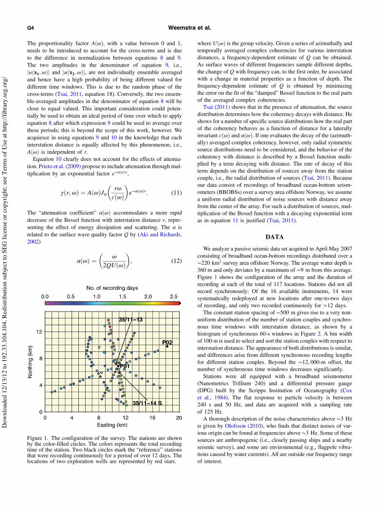
We analyze a passive seismic data set acquired in April-May 2007consisting of broadband ocean-bottom recordings distributed over a!220 km2 survey area offshore Norway. The average water depth is360 m and only deviates by a maximum of !9 m from this average.Figure 1 shows the configuration of the array and the duration ofrecording at each of the total of 117 locations. Stations did not allrecord synchronously: Of the 16 available instruments, 14 weresystematically redeployed at new locations after one-to-two daysof recording, and only two recorded continuously for >12 days.The constant station spacing of !500 m gives rise to a very non-

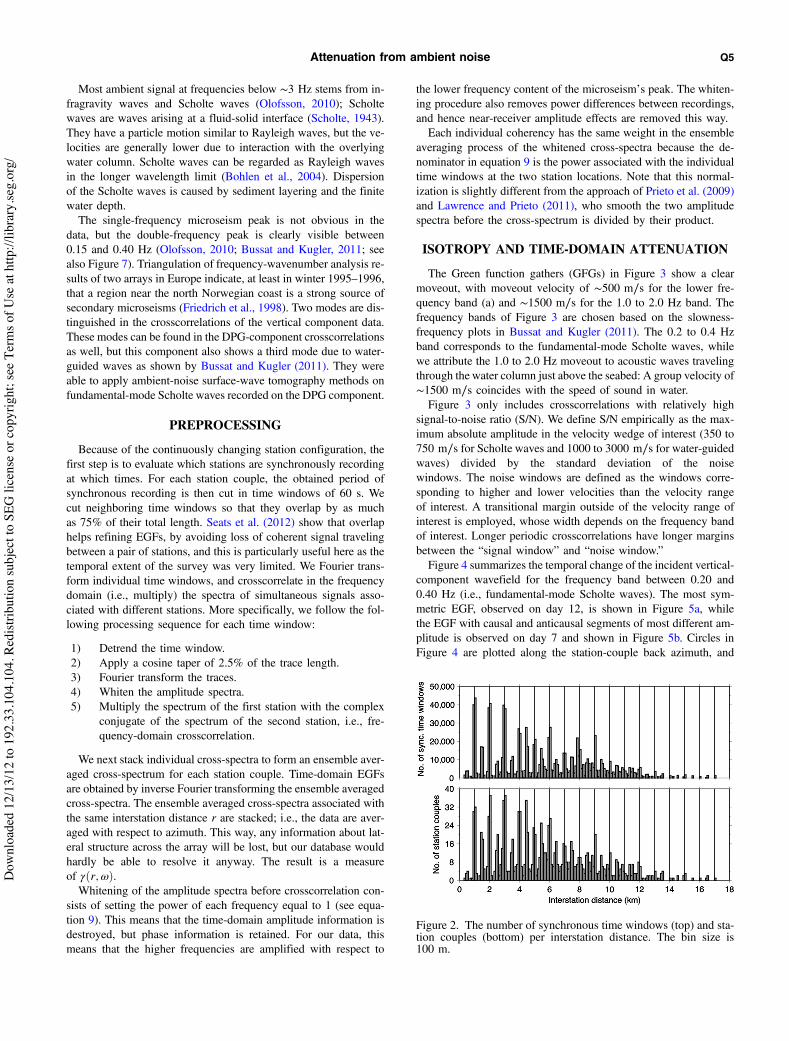
uniform distribution of the number of station couples and synchro-nous time windows with interstation distance, as shown by ahistogram of synchronous 60-s windows in Figure 2. A bin widthof 100 m is used to select and sort the station couples with respect tointerstation distance. The appearance of both distributions is similar,and differences arise from different synchronous recording lengthsfor different station couples. Beyond the !12; 000-m offset, thenumber of synchronous time windows decreases significantly.Stations were all equipped with a broadband seismometer

(Nanometrics Trillium 240) and a differential pressure gauge(DPG) built by the Scripps Institution of Oceanography (Coxet al., 1984). The flat response to particle velocity is between240 s and 50 Hz, and data are acquired with a sampling rateof 125 Hz.A thorough description of the noise characteristics above !3 Hz

is given by Olofsson (2010), who finds that distinct noises of var-ious origin can be found at frequencies above !3 Hz. Some of thesesources are anthropogenic (i.e., closely passing ships and a nearbyseismic survey), and some are environmental (e.g., flagpole vibra-tions caused by water currents). All are outside our frequency rangeof interest.

Figure 1. The configuration of the survey. The stations are shownby the color-filled circles. The colors represents the total recordingtime of the station. Two black circles mark the “reference” stationsthat were recording continuously for a period of over 12 days. Thelocations of two exploration wells are represented by red stars.

Q4 Weemstra et al.

Dow

nloa

ded

12/1

3/12

to 1

92.3

3.10

4.10

4. R

edist

ribut

ion

subj

ect t

o SE

G li

cens

e or

cop

yrig

ht; s

ee T

erm

s of U

se a

t http

://lib

rary

.seg.

org/

Most ambient signal at frequencies below !3 Hz stems from in-fragravity waves and Scholte waves (Olofsson, 2010); Scholtewaves are waves arising at a fluid-solid interface (Scholte, 1943).They have a particle motion similar to Rayleigh waves, but the ve-locities are generally lower due to interaction with the overlyingwater column. Scholte waves can be regarded as Rayleigh wavesin the longer wavelength limit (Bohlen et al., 2004). Dispersionof the Scholte waves is caused by sediment layering and the finitewater depth.The single-frequency microseism peak is not obvious in the

data, but the double-frequency peak is clearly visible between0.15 and 0.40 Hz (Olofsson, 2010; Bussat and Kugler, 2011; seealso Figure 7). Triangulation of frequency-wavenumber analysis re-sults of two arrays in Europe indicate, at least in winter 1995–1996,that a region near the north Norwegian coast is a strong source ofsecondary microseisms (Friedrich et al., 1998). Two modes are dis-tinguished in the crosscorrelations of the vertical component data.These modes can be found in the DPG-component crosscorrelationsas well, but this component also shows a third mode due to water-guided waves as shown by Bussat and Kugler (2011). They wereable to apply ambient-noise surface-wave tomography methods onfundamental-mode Scholte waves recorded on the DPG component.

PREPROCESSING

Because of the continuously changing station configuration, thefirst step is to evaluate which stations are synchronously recordingat which times. For each station couple, the obtained period ofsynchronous recording is then cut in time windows of 60 s. Wecut neighboring time windows so that they overlap by as muchas 75% of their total length. Seats et al. (2012) show that overlaphelps refining EGFs, by avoiding loss of coherent signal travelingbetween a pair of stations, and this is particularly useful here as thetemporal extent of the survey was very limited. We Fourier trans-form individual time windows, and crosscorrelate in the frequencydomain (i.e., multiply) the spectra of simultaneous signals asso-ciated with different stations. More specifically, we follow the fol-lowing processing sequence for each time window:

1) Detrend the time window.2) Apply a cosine taper of 2.5% of the trace length.3) Fourier transform the traces.4) Whiten the amplitude spectra.5) Multiply the spectrum of the first station with the complex

conjugate of the spectrum of the second station, i.e., fre-quency-domain crosscorrelation.

We next stack individual cross-spectra to form an ensemble aver-aged cross-spectrum for each station couple. Time-domain EGFsare obtained by inverse Fourier transforming the ensemble averagedcross-spectra. The ensemble averaged cross-spectra associated withthe same interstation distance r are stacked; i.e., the data are aver-aged with respect to azimuth. This way, any information about lat-eral structure across the array will be lost, but our database wouldhardly be able to resolve it anyway. The result is a measureof (!r;&".Whitening of the amplitude spectra before crosscorrelation con-

sists of setting the power of each frequency equal to 1 (see equa-tion 9). This means that the time-domain amplitude information isdestroyed, but phase information is retained. For our data, thismeans that the higher frequencies are amplified with respect to

the lower frequency content of the microseism’s peak. The whiten-ing procedure also removes power differences between recordings,and hence near-receiver amplitude effects are removed this way.Each individual coherency has the same weight in the ensemble

averaging process of the whitened cross-spectra because the de-nominator in equation 9 is the power associated with the individualtime windows at the two station locations. Note that this normal-ization is slightly different from the approach of Prieto et al. (2009)and Lawrence and Prieto (2011), who smooth the two amplitudespectra before the cross-spectrum is divided by their product.

ISOTROPY AND TIME-DOMAIN ATTENUATION

The Green function gathers (GFGs) in Figure 3 show a clearmoveout, with moveout velocity of !500 m$s for the lower fre-quency band (a) and !1500 m$s for the 1.0 to 2.0 Hz band. Thefrequency bands of Figure 3 are chosen based on the slowness-frequency plots in Bussat and Kugler (2011). The 0.2 to 0.4 Hzband corresponds to the fundamental-mode Scholte waves, whilewe attribute the 1.0 to 2.0 Hz moveout to acoustic waves travelingthrough the water column just above the seabed: A group velocity of!1500 m$s coincides with the speed of sound in water.Figure 3 only includes crosscorrelations with relatively high

signal-to-noise ratio (S/N). We define S/N empirically as the max-imum absolute amplitude in the velocity wedge of interest (350 to750 m$s for Scholte waves and 1000 to 3000 m$s for water-guidedwaves) divided by the standard deviation of the noisewindows. The noise windows are defined as the windows corre-sponding to higher and lower velocities than the velocity rangeof interest. A transitional margin outside of the velocity range ofinterest is employed, whose width depends on the frequency bandof interest. Longer periodic crosscorrelations have longer marginsbetween the “signal window” and “noise window.”Figure 4 summarizes the temporal change of the incident vertical-

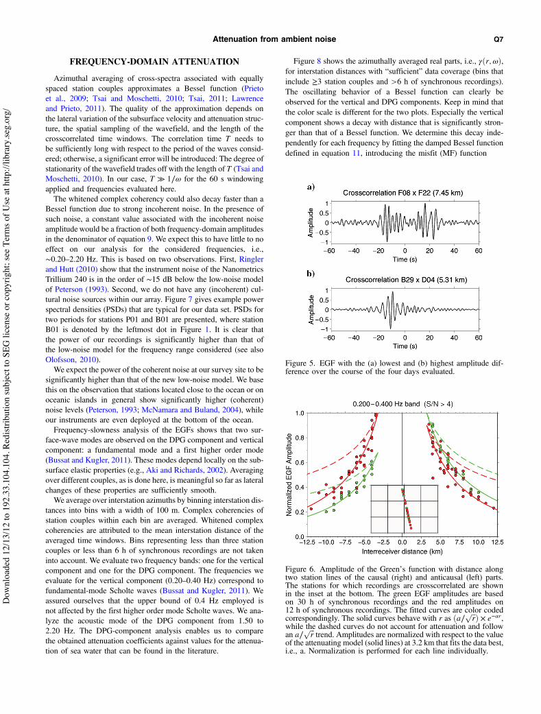
component wavefield for the frequency band between 0.20 and0.40 Hz (i.e., fundamental-mode Scholte waves). The most sym-metric EGF, observed on day 12, is shown in Figure 5a, whilethe EGF with causal and anticausal segments of most different am-plitude is observed on day 7 and shown in Figure 5b. Circles inFigure 4 are plotted along the station-couple back azimuth, and

Figure 2. The number of synchronous time windows (top) and sta-tion couples (bottom) per interstation distance. The bin size is100 m.

Attenuation from ambient noise Q5

Dow

nloa

ded

12/1

3/12

to 1

92.3

3.10

4.10

4. R

edist

ribut

ion

subj

ect t

o SE

G li

cens

e or

cop

yrig

ht; s

ee T

erm

s of U

se a

t http

://lib

rary

.seg.

org/

hence point toward the half-plane where the mostenergy is generated. In terms of source distribu-tions, this can be either a small region with a highvolume density of force or a broad region withonly a slight increase in volume density of force.These two end members are indistinguishablebased on one EGF alone.From Figure 4, one can in principle estimate

the average direction of propagation, and relativestrength of the ambient wavefield. This is in turndetermined by a number of factors. First, thesource distribution: Note, e.g., that a fully isotro-pic wavefield would result in circles associatedwith station couples all falling in the center ofthe polar plot, independent of azimuth. The sec-ond factor is the change of this source distribu-tion over time because EGFs represent differentperiods of one day. The third factor is the arrayconfiguration. The fourth factor is the interstationdistance, with the associated amplitude attenua-tion caused by geometrical spreading as well asattenuation due to the medium properties. Final-ly, the vertical and lateral structure of the subsur-face can change the amount of decay from placeto place through differences in attenuation. Wedefine attenuation here as the sum of “scattering”and “intrinsic” (i.e., absorption of energy) at-tenuation as we are unable to separate the two.Our goal with this study is to try to isolate at-

tenuation effects, and, if possible, the differencebetween attenuation due to geometrical spread-ing and attenuation due to medium properties,from all other factors. To evaluate whether thisis possible, we select two subsets of high-S/N(>4) synchronous EGFs, each correspondingto stations lying along one straight line (at inter-station distances >3.2 km). We plot in Figure 6EGF amplitude as a function of interstation dis-tance. Importantly, there is no temporal variationof the source distribution between stations of thesame subset because all EGFs are based on thesame period (> 4 h) of recording. We next com-pare these EGF amplitudes to amplitude decayproportional to a$

###r

pcaused by simple geome-

trical spreading (dashed lines) and amplitude de-cay proportional to a$

###r

p! e#)r (solid lines).

The latter model accounts for scattering and dis-sipation of energy of the ambient field. The con-stant a and attenuation coefficient ) are found byminimizing the L1-norm of the differences be-tween datapoints and the a$

###r

p! e#)r curves.

Figure 6 clearly suggests that the EGFs’ ampli-tudes decay faster than with

###r

pand that an at-

tenuating model explains the data better forcausal and anticausal parts of all data subsets.We conclude that attenuation effects other thansimple geometrical spreading can be inferredfrom the data, and we proceed to evaluate themquantitatively.

Figure 4. Polar plots show the difference between the amplitude of causal and anticausalparts of the EGFs, for four example days of recording, with each panel corresponding toone day. We only take into account here vertical-component crosscorrelations based onsynchronous recordings >4 h, interstation distances >3.2 km, and a S=N > 4, and wenormalize each of them individually to a maximum amplitude of 1. Station couples thatfulfilled these criteria are connected by lines in the inset maps. Each dot in a polar plotcorresponds to one station couple, its angular coordinate coinciding with the station-couple back azimuth, and its distance from the center of the plot proportional to thedifference between the causal and anticausal amplitude. Red dots correspond to thecrosscorrelations shown in Figure 5.

Figure 3. GFG of the vertical component for 0.2 to 0.4 Hz (a) and of the DPG com-ponent for 1.0 to 2.0 Hz (b). Only crosscorrelations based on synchronous recordings ofmore than 4 h, interstation distances of more than 3.2 km, and S=N > 4 are displayed.

Q6 Weemstra et al.

Dow

nloa

ded

12/1

3/12

to 1

92.3

3.10

4.10

4. R

edist

ribut

ion

subj

ect t

o SE

G li

cens

e or

cop

yrig

ht; s

ee T

erm

s of U

se a

t http

://lib

rary

.seg.

org/

FREQUENCY-DOMAIN ATTENUATION

Azimuthal averaging of cross-spectra associated with equallyspaced station couples approximates a Bessel function (Prietoet al., 2009; Tsai and Moschetti, 2010; Tsai, 2011; Lawrenceand Prieto, 2011). The quality of the approximation depends onthe lateral variation of the subsurface velocity and attenuation struc-ture, the spatial sampling of the wavefield, and the length of thecrosscorrelated time windows. The correlation time T needs tobe sufficiently long with respect to the period of the waves consid-ered; otherwise, a significant error will be introduced: The degree ofstationarity of the wavefield trades off with the length of T (Tsai andMoschetti, 2010). In our case, T % 1$& for the 60 s windowingapplied and frequencies evaluated here.The whitened complex coherency could also decay faster than a

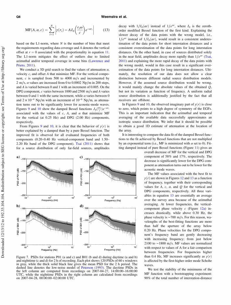
Bessel function due to strong incoherent noise. In the presence ofsuch noise, a constant value associated with the incoherent noiseamplitude would be a fraction of both frequency-domain amplitudesin the denominator of equation 9. We expect this to have little to noeffect on our analysis for the considered frequencies, i.e.,!0.20–2.20 Hz. This is based on two observations. First, Ringlerand Hutt (2010) show that the instrument noise of the NanometricsTrillium 240 is in the order of !15 dB below the low-noise modelof Peterson (1993). Second, we do not have any (incoherent) cul-tural noise sources within our array. Figure 7 gives example powerspectral densities (PSDs) that are typical for our data set. PSDs fortwo periods for stations P01 and B01 are presented, where stationB01 is denoted by the leftmost dot in Figure 1. It is clear thatthe power of our recordings is significantly higher than that ofthe low-noise model for the frequency range considered (see alsoOlofsson, 2010).We expect the power of the coherent noise at our survey site to be

significantly higher than that of the new low-noise model. We basethis on the observation that stations located close to the ocean or onoceanic islands in general show significantly higher (coherent)noise levels (Peterson, 1993; McNamara and Buland, 2004), whileour instruments are even deployed at the bottom of the ocean.Frequency-slowness analysis of the EGFs shows that two sur-

face-wave modes are observed on the DPG component and verticalcomponent: a fundamental mode and a first higher order mode(Bussat and Kugler, 2011). These modes depend locally on the sub-surface elastic properties (e.g., Aki and Richards, 2002). Averagingover different couples, as is done here, is meaningful so far as lateralchanges of these properties are sufficiently smooth.We average over interstation azimuths by binning interstation dis-

tances into bins with a width of 100 m. Complex coherencies ofstation couples within each bin are averaged. Whitened complexcoherencies are attributed to the mean interstation distance of theaveraged time windows. Bins representing less than three stationcouples or less than 6 h of synchronous recordings are not takeninto account. We evaluate two frequency bands: one for the verticalcomponent and one for the DPG component. The frequencies weevaluate for the vertical component (0.20–0.40 Hz) correspond tofundamental-mode Scholte waves (Bussat and Kugler, 2011). Weassured ourselves that the upper bound of 0.4 Hz employed isnot affected by the first higher order mode Scholte waves. We ana-lyze the acoustic mode of the DPG component from 1.50 to2.20 Hz. The DPG-component analysis enables us to comparethe obtained attenuation coefficients against values for the attenua-tion of sea water that can be found in the literature.

Figure 8 shows the azimuthally averaged real parts, i.e., (!r;&",for interstation distances with “sufficient” data coverage (bins thatinclude &3 station couples and >6 h of synchronous recordings).The oscillating behavior of a Bessel function can clearly beobserved for the vertical and DPG components. Keep in mind thatthe color scale is different for the two plots. Especially the verticalcomponent shows a decay with distance that is significantly stron-ger than that of a Bessel function. We determine this decay inde-pendently for each frequency by fitting the damped Bessel functiondefined in equation 11, introducing the misfit (MF) function

Figure 5. EGF with the (a) lowest and (b) highest amplitude dif-ference over the course of the four days evaluated.

Figure 6. Amplitude of the Green’s function with distance alongtwo station lines of the causal (right) and anticausal (left) parts.The stations for which recordings are crosscorrelated are shownin the inset at the bottom. The green EGF amplitudes are basedon 30 h of synchronous recordings and the red amplitudes on12 h of synchronous recordings. The fitted curves are color codedcorrespondingly. The solid curves behave with r as !a$

###r

p" ! e#)r,

while the dashed curves do not account for attenuation and followan a$

###r

ptrend. Amplitudes are normalized with respect to the value

of the attenuating model (solid lines) at 3.2 km that fits the data best,i.e., a. Normalization is performed for each line individually.

Attenuation from ambient noise Q7

Dow

nloa

ded

12/1

3/12

to 1

92.3

3.10

4.10

4. R

edist

ribut

ion

subj

ect t

o SE

G li

cens

e or

cop

yrig

ht; s

ee T

erm

s of U

se a

t http

://lib

rary

.seg.

org/

MF!A; ); c" $XN

i$1

(((((!ri" # AJ0

!ri&c

"e#)ri

(((( (13)

based on the L1-norm, where N is the number of bins that meetthe requirements regarding data coverage and A denotes the verticaloffset at r $ 0 associated with the proportionality in equation 11.The L1-norm mitigates the effect of outliers due to limitedazimuthal and/or temporal coverage in some bins (Lawrence andPrieto, 2011).We conduct a 3D grid search to find the values of attenuation ),

velocity c, and offset A that minimize MF. For the vertical compo-nent, c is sampled from 500 to 4000 m$s and incremented by2 m$s, ) values are increased from 0 to 0.0002 Np$m in 200 steps,and A is varied between 0 and 1 with an increment of 0.005. On theDPG component, c varies between 1000 and 2500 m$s and A variesbetween 0 and 1 with the same increment, while ) varies between 0and 2 ! 10#4 Np$m with an increment of 10#6 Np$m, as attenua-tion turns out to be significantly lower for acoustic-mode waves.Figures 9 and 10 show the damped Bessel functions J0!&ric "e

#)ri

associated with the values of c, A, and ) that minimize MFfor the vertical (at 0.25 Hz) and DPG (2.00 Hz) components,respectively.From Figures 9 and 10, it is clear that the behavior of (!r" is

better explained by a damped than by a pure Bessel function. Theimproved fit is observed for all evaluated frequencies of bothcomponents (0.20–0.40 Hz vertical-component band and 1.50–2.20 Hz band of the DPG component). Tsai (2011) shows thatfor a source distribution of only far-field sources, amplitudes

decay with 1$I0!)r" instead of 1$e)r, where I0 is the zeroth-order modified Bessel function of the first kind. Explaining theslower decay of the data points with the wrong model, i.e.,1$e)r instead of 1$I0!)r", would result in a consistent underes-timation of the data points for short interstation distances and aconsistent overestimation of the data points for long interstationdistances. On the other hand, in case of sources distributed solelyin the near field, amplitudes decay more rapidly than 1$e)r (Tsai,2011) and explaining the more rapid decay of the data points withthe wrong model, would in this case result in a significant over-estimation of the data points for long interstation distances. Ulti-mately, the resolution of our data does not allow a cleardistinction between different radial source distribution models.However, if the assumed source distribution would be wrong,it would mainly change the absolute values of the obtained Q,but not its variation as function of frequency. A uniform radialsource distribution is additionally justified by the fact that allreceivers are offshore.In Figures 9 and 10, the observed imaginary part of (!r" is close

to zero, which points to a high degree of symmetry of the EGFs.This is an important indication that the azimuthal and temporalaveraging of the available data successfully approximates anisotropic source distribution. We infer that it should be possibleto obtain a good 1D estimate of attenuation at the location ofthe array.It is interesting to compare the data fit of the damped Bessel func-

tions to the fit achieved by Bessel functions that are not multipliedby an exponential term (i.e., MF is minimized with ) set to 0). Fit-ting damped instead of pure Bessel functions (Figure 11) gives an

overall decrease of MF for the vertical and DPGcomponent of 58% and 17%, respectively. Thedecrease is significantly lower for the DPG com-ponent as attenuation turns out to be lower for theacoustic mode waves.The MF values associated with the best fit to

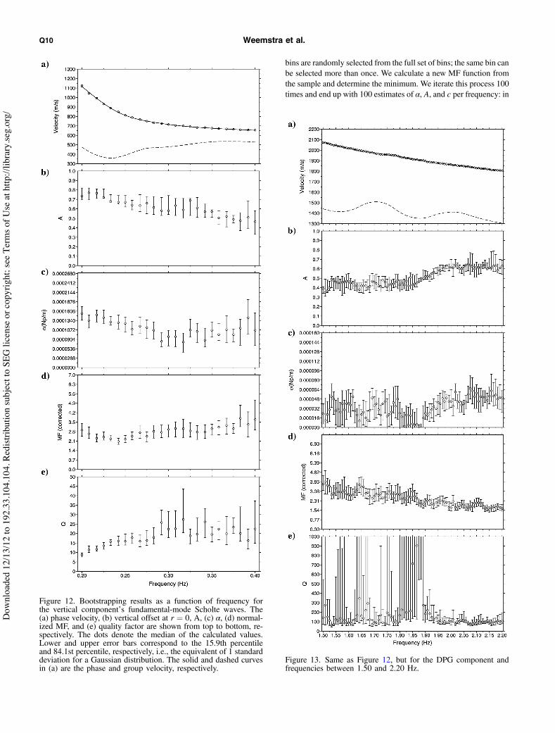
(!r" are shown in Figures 12 and 13 as a functionof frequency, together with their correspondingvalues for A, c, ), and Q for the vertical andDPG components, respectively. All three vari-ables in equation 13 are essentially an averageover the survey area because of the azimuthalaveraging. At lower frequencies, the vertical-component phase velocity c (Figure 12a) in-creases drastically, while above 0.30 Hz, thephase velocity is !700 m$s. For this reason, wa-velengths of the best-fitting functions are morethan half the aperture of the array below0.20 Hz. Phase velocities for the DPG compo-nent’s frequency band are gently decreasingwith increasing frequency; from just below2100 to !1800 m$s. MF values are normalizedwith respect to values of A for a fair comparisonbetween frequencies. For frequencies higherthan 0.4 Hz, MF increases significantly as (!r"is affected by the first-higher order mode Scholtewaves.We test the stability of the minimums of the

MF function with a bootstrapping experiment:90% of the total number of interstation-distance

Figure 7. PSDs for stations P01 (a and c) and B01 (b and d) during daytime (a and b)and nighttime (c and d) for 2 h of recording. Each plot shows 120 PSDs of 60 s windowsin gray, while the thick solid black line gives the mean PSD for the 2 h period. Thedashed line denotes the low-noise model of Peterson (1993). The daytime PSDs inthe left column are computed from recordings on 2007-04-27, 14:00:00–16:00:00UTC, while the nighttime PSDs in the right column are calculated from recordingson 2007-04-28, 00:00:00–02:00:00 UTC.

Q8 Weemstra et al.

Dow

nloa

ded

12/1

3/12

to 1

92.3

3.10

4.10

4. R

edist

ribut

ion

subj

ect t

o SE

G li

cens

e or

cop

yrig

ht; s

ee T

erm

s of U

se a

t http

://lib

rary

.seg.

org/

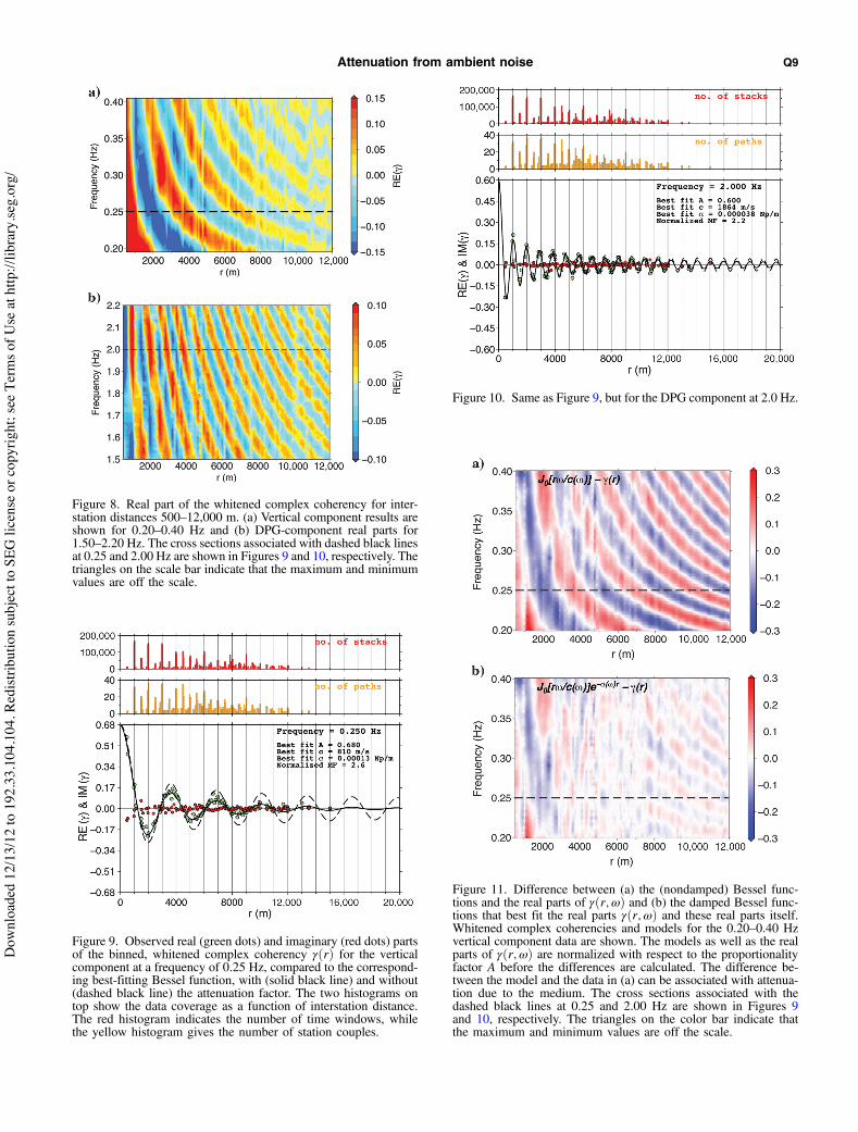
Figure 9. Observed real (green dots) and imaginary (red dots) partsof the binned, whitened complex coherency (!r" for the verticalcomponent at a frequency of 0.25 Hz, compared to the correspond-ing best-fitting Bessel function, with (solid black line) and without(dashed black line) the attenuation factor. The two histograms ontop show the data coverage as a function of interstation distance.The red histogram indicates the number of time windows, whilethe yellow histogram gives the number of station couples.

Figure 10. Same as Figure 9, but for the DPG component at 2.0 Hz.

Figure 11. Difference between (a) the (nondamped) Bessel func-tions and the real parts of (!r;&" and (b) the damped Bessel func-tions that best fit the real parts (!r;&" and these real parts itself.Whitened complex coherencies and models for the 0.20–0.40 Hzvertical component data are shown. The models as well as the realparts of (!r;&" are normalized with respect to the proportionalityfactor A before the differences are calculated. The difference be-tween the model and the data in (a) can be associated with attenua-tion due to the medium. The cross sections associated with thedashed black lines at 0.25 and 2.00 Hz are shown in Figures 9and 10, respectively. The triangles on the color bar indicate thatthe maximum and minimum values are off the scale.

Figure 8. Real part of the whitened complex coherency for inter-station distances 500–12,000 m. (a) Vertical component results areshown for 0.20–0.40 Hz and (b) DPG-component real parts for1.50–2.20 Hz. The cross sections associated with dashed black linesat 0.25 and 2.00 Hz are shown in Figures 9 and 10, respectively. Thetriangles on the scale bar indicate that the maximum and minimumvalues are off the scale.

Attenuation from ambient noise Q9

Dow

nloa

ded

12/1

3/12

to 1

92.3

3.10

4.10

4. R

edist

ribut

ion

subj

ect t

o SE

G li

cens

e or

cop

yrig

ht; s

ee T

erm

s of U

se a

t http

://lib

rary

.seg.

org/

bins are randomly selected from the full set of bins; the same bin canbe selected more than once. We calculate a new MF function fromthe sample and determine the minimum. We iterate this process 100times and end up with 100 estimates of ), A, and c per frequency: in

Figure 12. Bootstrapping results as a function of frequency forthe vertical component’s fundamental-mode Scholte waves. The(a) phase velocity, (b) vertical offset at r $ 0, A, (c) ), (d) normal-ized MF, and (e) quality factor are shown from top to bottom, re-spectively. The dots denote the median of the calculated values.Lower and upper error bars correspond to the 15.9th percentileand 84.1st percentile, respectively, i.e., the equivalent of 1 standarddeviation for a Gaussian distribution. The solid and dashed curvesin (a) are the phase and group velocity, respectively.

Figure 13. Same as Figure 12, but for the DPG component andfrequencies between 1.50 and 2.20 Hz.

Q10 Weemstra et al.

Dow

nloa

ded

12/1

3/12

to 1

92.3

3.10

4.10

4. R

edist

ribut

ion

subj

ect t

o SE

G li

cens

e or

cop

yrig

ht; s

ee T

erm

s of U

se a

t http

://lib

rary

.seg.

org/

the ideal case of a perfectly constrained solution, these estimateswould all be equal.Phase velocities prove to be well constrained as bootstrapping

yields very little variability; error bars are coinciding with medianvalues and hence are hardly visible for both components (Figures 12aand 13a). The bootstrapping does yield some variability in A and )values for both components. A slight trade-off between these twoparameters can be observed if we examine the cost functions’ MFassociated with the best fit to (!r" and fix the phase velocity c. Forthe lower frequencies in the vertical-component frequency band,i.e., toward 0.20 Hz and hence on the slope of the double-frequencymicroseism peak (Peterson, 1993), values for A tend to be higher.This points to a lower power associated with the cross-terms, whichin turn indicates that the differences in power of different sourcesare low for these frequencies. The DPG-component frequency bandshows the same for the higher frequencies.The attenuation coefficient, ), associated with the best fit of MF

to (!r" is presented in Figures 12c and 13c as a function of fre-quency and for the vertical and DPG component, respectively.The quality factors associated with these decay values are shownin Figures 12e and 13e, respectively. Calculating the quality factorsfrom ) according to equation 12 requires knowledge of the groupvelocity U. We determine U by differentiating numerically our ob-served phase-velocity dispersion curve (Aki and Richards, 2002).The vertical component’s group velocity varies around 500 m$swith an increasing trend, while the DPG component’s groupvelocity varies around 1400 m$s with a decreasing trend (seeFigures 12a and 13a, respectively). These values are in agreementwith the observed moveouts in Figure 3.Figure 13e shows that surface wave quality factor as a function of

frequency oscillates around a mean value of !100 for the DPG com-ponent. As attenuation for this component turns out to be so low, asignificant number of the bootstrapping samples yield an attenua-tion coefficient equal to zero for some frequencies; this is associatedwith error bars on the correspondingQ values reaching infinity. Var-iations become less severe with increasing frequency, however. Thevertical component Q (Figure 12e) oscillates around !20, and itdecreases with decreasing frequency below 0.30 Hz.

COMPARISON WITH OTHER STUDIES

Temporal and azimuthal averaging of spectral whitened datagives us realistic frequency-dependent estimates of Q, and we inferthat our method correctly extracts this information from the ambientseismic field. Our results show that the ambient seismic field carriessignificant information about the anelastic earth structure. This hasbeen shown before (Prieto et al., 2009; Lawrence and Prieto, 2011;Lin et al., 2011) but not for the spatial and temporal dimensionspresented here.The bulk of the Scholte and acoustic guided wave analysis per-

formed is based on shallow-water data, i.e., <100 m (Bohlen et al.,2004; Klein et al., 2005; Zhou et al., 2009). The great water depth ofthis survey (!360 m) causes a downward frequency shift of themodal transitions. Greater depths are able to accommodate lowerfrequency Scholte and acoustic wave modes. Forward modelingby Klein et al. (2005) indicates that an overlying water columnof several hundred meters would be able to support acoustic guidedwaves below 1 Hz. This is exactly what we observe for this data set.We will shortly discuss the obtained velocity and attenuation

estimates for the respective components and the relation to the localgeology.

DPG-component frequency band

The phase velocities we obtain for the acoustic guided waves are,to a first order, in agreement with values found by others (Kleinet al., 2005). Furthermore, the group velocity to be expected forthe conditions of our survey is about 1478 m$s. We use Macken-zie’s equation for the speed of sound in sea water (Mackenzie,1981) using a depth of 360 m, a temperature of 5°C, and an averagesalinity of 36 ppt (Berx and Hughes, 2009) to obtain this value. Ourgroup velocity oscillates around this value, although it is a bit lowerfor the higher frequencies.The attenuation of acoustic guided waves for the frequencies con-

sidered here is still not fully understood, and quality factors in plainsea water are unknown for the frequencies considered here (Jensenet al., 2000). Because the DPGs are measuring pressure fluctuationsonly !50 cm above the sea bottom, it is unclear if or to what extentthe estimated phase velocities and attenuation values need to be as-sociated with sea-bed sediment estimates of these parameters. Asthe obtained attenuation coefficients are to a first-order constantwith frequency, we estimate the attenuation coefficient for theacoustic guided waves at 0.00004 Np$m. This corresponds to acompressional wave quality factor of about 100 (see Figure 13).Future investigations focusing on similar frequencies and environ-ments (water depth, temperature, salinity) have to confirm ourfindings.Contrary to the fundamental and first higher mode Scholte waves,

the slowness-frequency spectra of the vertical and transversal com-ponents do not show the acoustic guided waves (Bussat and Kugler,2011). The radial component does record the acoustic guidedwaves, however. This indeed suggests a possible interaction of thesewaves with the sea-bottom sediments. The very shallow sediments(upper !5 m) act as a purely compressional medium because of thehigh water content (Jensen et al., 2000; Zhou et al., 2009). In gen-eral, the sound speed of these sediment sampling acoustic waves isonly slightly higher than the speed of sound in sea water, with theirratio approaching one with increasing frequency (Klein et al.,2005). It would be interesting to estimate phase velocities and qual-ity factors for the radial component in a similar fashion as the onesobtained for the DPG component and compare the parameters forthe two different components. This is, however, beyond the scope ofthis investigation.

Vertical component frequency band

Anelastic attenuation of Scholte waves is poorly addressed for thelow frequencies considered here. Broadhead et al. (1993) analyzeScholte wave attenuation at two sites off the coast of the westernUnited States. For water depths of 2600 and 3800 m, they find aver-age quality factors of about 30–40 for a frequency range of 0.3 to6.0 Hz. They expect, however, that the obtained Qs are biased tolower frequencies. The higher frequencies in the fundamental-modeScholte wave frequency band give us surface wave quality factorsaround 20 (see Figure 12e), which is in good agreement with theirvalues.Nguyen et al. (2009) analyze shot recordings from one broad-

band ocean-bottom survey located at the Ninetyeast Ridge in theIndian Ocean. They find that a surface wave quality factor of 40

Attenuation from ambient noise Q11

Dow

nloa

ded

12/1

3/12

to 1

92.3

3.10

4.10

4. R

edist

ribut

ion

subj

ect t

o SE

G li

cens

e or

cop

yrig

ht; s

ee T

erm

s of U

se a

t http

://lib

rary

.seg.

org/

is required for the uppermost mushy layer to explain the observedamplitude decay of the Scholte waves with distance. The uppermostlayer is relatively thin at the location they investigate, and the fre-quencies of the observed Scholte waves are significantly higher.Nevertheless, their value is in agreement with our estimates. Otherstudies evaluating Scholte wave attenuation end up with signifi-cantly higher estimates for surface wave quality factors (Bromirskiet al., 1992; Nolet and Dorman, 1996).

Relation to geology

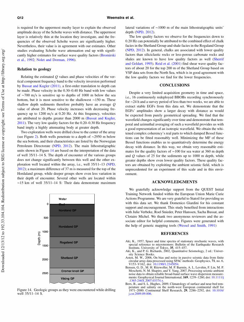
Relating the estimated Q values and phase velocities of the ver-tical component frequency band to the velocity inversion performedby Bussat and Kugler (2011), a first-order translation to depth canbe made. Phase velocity in the 0.30–0.40 Hz band with low valuesof !700 m$s is sensitive up to depths of 1000 m below the seabottom, but it is most sensitive to the shallowest !150 m. Theseshallow depth sediments therefore probably have an average Qvalue of about 20. Phase velocity increases with decreasing fre-quency up to 1200 m$s at 0.20 Hz. At this frequency, velocitiesare attributed to depths greater than 2000 m (Bussat and Kugler,2011). The very low quality factors for the 0.20–0.30 Hz frequencyband imply a highly attenuating body at greater depth.Two exploration wells were drilled close to the center of the array

(see Figure 2). Both wells penetrate to a depth of !2950 m belowthe sea bottom, and their characteristics are listed by the NorwegianPetroleum Directorate (NPD, 2012). The main lithostratigraphicunits shown in Figure 14 are based on the interpretation of the dataof well 35/11–14 S. The depth of encounter of the various groupsdoes not change significantly between this well and the other ex-ploration well located within the array, i.e., well 35/11–13 (NPD,2012); a maximum difference of 37 m is measured for the top of theHordaland group, while deeper groups show even less variation intheir depth of encounter. Several other wells are located within!15 km of well 35/11–14 S: Their data demonstrate maximum

lateral variations of !1000 m of the main lithostratigraphic units’depth (NPD, 2012).The low quality factors we observe for the frequencies down to

0.20 Hz can potentially be attributed to the combined effect of chalkfacies in the Shetland Group and shale facies in the Rogaland Group(NPD, 2012). In general, chalks are associated with lower qualityfactors than siliciclastic rocks or less-porous carbonate rocks andshales are known to have low quality factors as well (Sherrifand Geldart, 1995). Reid et al. (2001) find shear wave quality fac-tors of about 20 for the top 200 m of the Shetland Group based onVSP data sets from the North Sea, which is in good agreement withthe low quality factors we find for the lower frequencies.

CONCLUSIONS

Despite a very limited acquisition geometry in time and space,i.e., 16 continuously redeployed BBOBs recording synchronouslyfor !24 h and a survey period of less than two weeks, we are able toextract stable EGFs from this data set. We demonstrate that theEGFs’ amplitudes show a larger decay with distance as wouldbe expected from purely geometrical spreading. We find that thewavefield changes significantly over time and demonstrate that tem-poral and azimuthal averaging of such a wavefield provides us witha good representation of an isotropic wavefield. We obtain the whi-tened complex coherency’s real parts to which damped Bessel func-tions can be fitted reasonably well. Minimizing the MF of theseBessel functions enables us to quantitatively determine the energydecay with distance. In this way, we obtain very reasonable esti-mates for the quality factors of !100 for sea water at 360 m depthand Q values of 25 for the sediments up to 1000 m depth, whilegreater depths show even lower quality factors. These quality fac-tors are obtained by exploiting the ambient seismic field, which isunprecedented for an experiment of this scale and in this envir-onment.

ACKNOWLEDGMENTS

We gratefully acknowledge support from the QUEST InitialTraining Network funded within the European Union Marie CurieActions Programme. We are very grateful to Statoil for providing uswith this data set. We thank Domenico Giardini for his constantsupport and encouragement. This study benefited from interactionswith Julie Verbeke, Roel Snieder, Peter Hanssen, Sacha Bussat, andClotaire Michel. We thank two anonymous reviewers and the as-sociate editor for helpful comments. Figures were generated withthe help of generic mapping tools (Wessel and Smith, 1991)

REFERENCES

Aki, K., 1957, Space and time spectra of stationary stochastic waves, withspecial reference to microtremors: Bulletin of the Earthquake ResearchInstitute, University of Tokyo, 35, 415–457.

Aki, K., and P. G. Richards, 2002, Quantitative Seismology, 2 ed.: Univer-sity Science Books.

Asten, M. W., 2006, On bias and noise in passive seismic data from finitecircular array data processed using SPAC methods: Geophysics, 71, no. 6,V153–V162, doi: 10.1190/1.2345054.

Bensen, G. D., M. H. Ritzwoller, M. P. Barmin, A. L. Levshin, F. Lin, M. P.Moschetti, N. M. Shapiro, and Y. Yang, 2007, Processing seismic ambientnoise data to obtain reliable broad-band surface wave dispersion measure-ments: Geophysical Journal International, 169, 1239–1260, doi: 10.1111/j.1365-246X.2007.03374.x.

Berx, B., and S. L. Hughes, 2009, Climatology of surface and near-bed tem-perature and salinity on the north-west European continental shelf for1971–2000: Continental Shelf Research, 29, 2286–2292, doi: 10.1016/j.csr.2009.09.006.

Figure 14. Geologic groups as they were encountered while drillingwell 35/11–14 S.

Q12 Weemstra et al.

Dow

nloa

ded

12/1

3/12

to 1

92.3

3.10

4.10

4. R

edist

ribut

ion

subj

ect t

o SE

G li

cens

e or

cop

yrig

ht; s

ee T

erm

s of U

se a

t http

://lib

rary

.seg.

org/

Bohlen, T., S. Kugler, G. Klein, and F. Theilen, 2004, 1.5D inversion oflateral variation of Scholte-wave dispersion: Geophysics, 69, 330–344,doi: 10.1190/1.1707052.

Brenguier, F., N. M. Shapiro, M. Campillo, A. Nercessian, and V. Ferrazzini,2007, 3-D surface wave tomography of the Piton de la Fournaise volcanousing seismic noise correlations: Geophysical Research Letters, 34,L02305, doi: 10.1029/2006GL028586.

Broadhead, M., H. Ali, and L. Bibee, 1993, Scholte wave attenuationestimates from two diverse test sites: Proceedings of OCEANS’93 — Engineering in Harmony with Ocean, IEEE, volume 1,I114–I118.

Bromirski, P. D., L. N. Frazer, and F. K. Duennebier, 1992, Sedimentshear Q from airgun OBS data: Geophysical Journal International,110, 465–485, doi: 10.1111/j.1365-246X.1992.tb02086.x.

Bussat, S., and S. Kugler, 2009, Recording noise-estimating shear-wave ve-locities: Feasibility of offshore ambient-noise surface-wave tomography(ANSWT) on a reservoir scale: 79th Annual International Meeting, SEG,Expanded Abstracts, 1627–1631.

Bussat, S., and S. Kugler, 2011, Offshore ambient-noise surface-wave tomo-graphy above 0.1 Hz and its applications: The Leading Edge, 30, 514–524, doi: 10.1190/1.3589107.

Campillo, M., and A. Paul, 2003, Long-range correlations in the diffuse seis-mic coda: Science, 299, 547–549, doi: 10.1126/science.1078551.

Chapman, M., E. Liu, and X.-Y. Li, 2006, The influence of fluid-sensitivedispersion and attenuation on AVO analysis: Geophysical Journal Inter-national, 167, 89–105, doi: 10.1111/j.1365-246X.2006.02919.x.

Chávez-García, F. J., M. Rodríguez, and W. R. Stephenson, 2005, An alter-native approach to the SPAC analysis of microtremors: Exploiting statio-narity of noise: Bulletin of the Seismological Society of America, 95,277–293, doi: 10.1785/0120030179.

Claerbout, J. F., 1968, Synthesis of a layered medium from its acoustic trans-mission response: Geophysics, 33, 264–269, doi: 10.1190/1.1439927.

Cox, C., T. Deaton, and S. Webb, 1984, A deep-sea differential pressuregauge: Journal of Atmospheric and Oceanic Technology, 1, 237–246,doi: 10.1175/1520-0426(1984)001<0237:ADSDPG>2.0.CO;2.

Derode, A., E. Larose, M. Tanter, J. de Rosny, A. Tourin, M. Campillo, andM. Fink, 2003, Recovering the Green’s function from field-field correla-tions in an open scattering medium (L): Journal of the Acoustical Societyof America, 113, 2973–2976, doi: 10.1121/1.1570436.

Draganov, D., K. Wapenaar, W. Mulder, J. Singer, and A. Verdel, 2007, Re-trieval of reflections from seismic background-noise measurements: Geo-physical Research Letters, 34, L04305, doi: 10.1029/2006GL028735.

Duvall, T. L., S. M. Jefferies, J. W. Harvey, and M. A. Pomerantz, 1993,Time-distance helioseismology: Nature, 362, 430–432, doi: 10.1038/362430a0.

Ekström, G., G. A. Abers, and S. C. Webb, 2009, Determination of surface-wave phase velocities across USArray from noise and Aki’s spectral for-mulation: Geophysical Research Letters, 36, L18301, doi: 10.1029/2009GL039131.

Friedrich, A., F. Krüger, and K. Klinge, 1998, Ocean-generated microseis-mic noise located with the Gräfenberg array: Journal of Seismology, 2,no. 1, 47–64, doi: 10.1023/A:1009788904007.

Goertz, A., B. Schechinger, B. Witten, M. Koerbe, and P. Krajewski, 2012,Extracting subsurface information from ambient seismic noise — A casestudy from Germany: Geophysics, 77, no. 4, KS13–KS31, doi: 10.1190/geo2011-0306.1.

Hasselmann, K., 1963, A statistical analysis of the generation of microseisms:Reviews of Geophysics, 1, 177–210, doi: 10.1029/RG001i002p00177.

Jensen, F. B., W. A. Kuperman, M. B. Porter, and H. Schmidt, 2000, Com-putational ocean acoustics: Springer-Verlag.

Klein, G., T. Bohlen, F. Theilen, S. Kugler, and T. Forbriger, 2005, Acquisi-tion and inversion of dispersive seismic waves in shallow marine envir-onments: Marine Geophysical Researches, 26, no. 2, 287–315, doi: 10.1007/s11001-005-3725-6.

Landés, M., F. Hubans, N. M. Shapiro, A. Paul, and M. Campillo, 2010,Origin of deep ocean microseisms by using teleseismic body waves:Journal of Geophysical Research, 115, B05302, doi: 10.1029/2009JB006918.

Larose, E., L. Margerin, A. Derode, B. van Tiggelen, M. Campillo, N. Sha-piro, A. Paul, L. Stehly, and M. Tanter, 2006, Correlation of random wa-vefields: An interdisciplinary review: Geophysics, 71, no. 4, SI11–SI21,doi: 10.1190/1.2213356.

Lawrence, J. F., and G. A. Prieto, 2011, Attenuation tomography of thewestern United States from ambient seismic noise: Journal of GeophysicalResearch, 116, B06302, doi: 10.1029/2010JB007836.

Lin, F.-C., M. H. Ritzwoller, andW. Shen, 2011, On the reliability of attenua-tion measurements from ambient noise cross-correlations: GeophysicalResearch Letters, 38, L11303, doi: 10.1029/2011GL047366.

Lobkis, O. I., and R. L. Weaver, 2001, On the emergence of the Green’sfunction in the correlations of a diffuse field: The Journal of the Acous-tical Society of America, 110, 3011–3017, doi: 10.1121/1.1417528.

Longuet-Higgins, M. S., 1950, A theory of the origin of microseisms: Phi-losophical Transactions of the Royal Society of London, Series A, Math-ematical and Physical Sciences, 243, 1–35, doi: 10.1098/rsta.1950.0012.

Mackenzie, K. V., 1981, Nine term equation for sound speed in the oceans:Journal of the Acoustical Society of America, 70, 807–812, doi: 10.1121/1.386920.

McNamara, D. E., and R. P. Buland, 2004, Ambient noise levels in the con-tinental United States: Bulletin of the Seismological Society of America,94, 1517–1527, doi: 10.1785/012003001.

Nakahara, H., 2012, Formulation of the spatial autocorrelation (SPAC)method in dissipative media: Geophysical Journal International, 190,1777–1783, doi: 10.1111/j.1365-246X.2012.05591.x.

Nguyen, X., T. Dahm, and I. Grevemeyer, 2009, Inversion of Scholte wavedispersion and waveform modeling for shallow structure of the NinetyeastRidge: Journal of Seismology, 13, no. 4, 543–559, doi: 10.1007/s10950-008-9145-8.

Nolet, G., and L. M. Dorman, 1996, Waveform analysis of Scholte modes inocean sediment layers: Geophysical Journal International, 125, 385–396,doi: 10.1111/j.1365-246X.1996.tb00006.x.

NPD, 2012, Norwegian petroleum directorate factpages, http://factpages.npd.no/factpages/default.aspx, accessed 19 March, 2012.

Okada, H., 2003, The microtremor survey method, No. 12: SEG.Olofsson, B., 2010, Marine ambient seismic noise in the frequency range1–10 Hz: The Leading Edge, 29, 418–435, doi: 10.1190/1.3378306.

Peterson, J., 1993, Observation and modeling of seismic background noise:U.S. Geological Survey Open-File Report, 93–322.

Poli, P., H. A. Pedersen, and M. Campillo, and the POLENET/LAPNETWorking Group, 2012, Emergence of body waves from cross-correlationof short period seismic noise: Geophysical Journal International, 188,549–558, doi: 10.1111/j.1365-246X.2011.05271.x.

Prieto, G. A., J. F. Lawrence, and G. C. Beroza, 2009, Anelastic Earthstructure from the coherency of the ambient seismic field: Journal ofGeophysical Research, 114, B07303, doi: 10.1029/2008JB006067.

Reid, F. J. L., P. H. Nguyen, C. MacBeth, and R. A. Clark, 2001,Q estimatesfrom North Sea VSPs: 71st Annual International Meeting, SEG, Ex-panded Abstracts, 440–443.

Rickett, J., and J. Claerbout, 1999, Acoustic daylight imaging via spectralfactorization; helioseismology and reservoir monitoring: The LeadingEdge, 18, 957–960, doi: 10.1190/1.1438420.

Ringler, A. T., and C. R. Hutt, 2010, Self-noise models of seismic instru-ments: Seismological Research Letters, 81, 972–983, doi: 10.1785/gssrl.81.6.972.

Roux, P., K. G. Sabra, P. Gerstoft, W. A. Kuperman, and M. C. Fehler, 2005,P-waves from cross-correlation of seismic noise: Geophysical ResearchLetters, 32, L19303, doi: 10.1029/2005GL023803.

Scholte, J., 1943, Over het verband tussen zeegolven en microseismen, I andII: Verslag Nederlands Akademie van Wetenschappen, 52, 669–683.

Seats, K. J., J. F. Lawrence, and G. A. Prieto, 2012, Improved ambient noisecorrelation functions using Welch’s method: Geophysical Journal Inter-national, 188, 513–523, doi: 10.1111/j.1365-246X.2011.05263.x.

Shapiro, N. M., and M. Campillo, 2004, Emergence of broadband Rayleighwaves from correlations of the ambient seismic noise: Geophysical Re-search Letters, 31, L07614, doi: 10.1029/2004GL019491.

Shapiro, N. M., M. Campillo, L. Stehly, and M. H. Ritzwoller, 2005, High-resolution surface-wave tomography from ambient seismic noise:Science, 307, 1615–1618, doi: 10.1126/science.1108339.

Sherrif, R. E., and L. P. Geldart, 1995, Exploration seismology (second edi-tion): Cambridge University Press.

Snieder, R., 2004, Extracting the Green’s function from the correlation ofcoda waves: a derivation based on stationary phase: Physical Review E,69, no. 4, 046610, doi: 10.1103/PhysRevE.69.046610.

Snieder, R., K. Wapenaar, and U. Wegler, 2007, Unified Green’s functionretrieval by cross-correlation; connection with energy principles: PhyscalReview E, 75, 036103, doi: 10.1103/PhysRevE.75.036103.

Stehly, L., M. Campillo, and N. M. Shapiro, 2006, A study of the seismicnoise from its long-range correlation properties: Journal of GeophysicalResearch, 111, B10306, doi: 10.1029/2005JB004237.

Tsai, V. C., 2009, On establishing the accuracy of noise tomography travel-time measurements in a realistic medium: Geophysical Journal Interna-tional, 178, 1555–1564, doi: 10.1111/j.1365-246X.2009.04239.x.

Tsai, V. C., 2011, Understanding the amplitudes of noise correlation mea-surements: Journal of Geophysical Research, 116, B09311, doi: 10.1029/2011JB008483.

Tsai, V. C., and M. P. Moschetti, 2010, An explicit relationship betweentime-domain noise correlation and spatial autocorrelation (SPAC) results:Geophysical Journal International, 182, 454–460, doi: 10.1111/j.1365-246X.2010.04633.x.

Wapenaar, C., D. Draganav, R. Snieder, X. Campman, and A. Verdel, 2010,Tutorial on seismic interferometry: Part 1 — Basic principles and appli-cations: Geophysics, 75, no. 5, 75A195–75A209, doi: 10.1190/1.3457445.

Attenuation from ambient noise Q13

Dow

nloa

ded

12/1

3/12

to 1

92.3

3.10

4.10

4. R

edist

ribut

ion

subj

ect t

o SE

G li

cens

e or

cop

yrig

ht; s

ee T

erm

s of U

se a

t http

://lib

rary

.seg.

org/

Wapenaar, K., 2004, Retrieving the elastodynamic Green’s function of anarbitrary inhomogeneous medium by cross correlation: Physical ReviewLetters, 93, 254301, doi: 10.1103/PhysRevLett.93.254301.

Wessel, P., and W. H. F. Smith, 1991, Free software helps map and displaydata: EOS Transactions of the AGU, 72, 441, doi: 10.1029/90EO00319.

Yang, Y., and M. H. Ritzwoller, 2008, Characteristics of ambient seismicnoise as a source for surface wave tomography: Geochemistry, Geophysics,Geosystems, 9, Q02008, doi: 10.1029/2007GC001814.

Yang, Y., M. H. Ritzwoller, A. L. Levshin, and N. M. Shapiro, 2007,Ambient noise Rayleigh wave tomography across Europe: Geophysical Jour-nal International, 168, 259–274, doi: 10.1111/j.1365-246X.2006.03203.x.

Yokoi, T., and S. Margaryan, 2008, Consistency of the spatial autocorrela-tion method with seismic interferometry and its consequence: Geo-physical Prospecting, 56, 435–451, doi: 10.1111/j.1365-2478.2008.00709.x.

Zhang, J., P. Gerstoft, and P. M. Shearer, 2009, High-frequency P-wave seis-mic noise driven by ocean winds: Geophysical Research Letters, 36,L09302, doi: 10.1029/2009GL037761.

Zhou, J.-X., X.-Z. Zhang, and D. P. Knobles, 2009, Low-frequency geo-acoustic model for the effective properties of sandy seabottoms: Journalof the Acoustical Society of America, 125, 2847–2866, doi: 10.1121/1.3089218.

Q14 Weemstra et al.

Dow

nloa

ded

12/1

3/12

to 1

92.3

3.10

4.10

4. R

edist

ribut

ion

subj

ect t

o SE

G li

cens

e or

cop

yrig

ht; s

ee T

erm

s of U

se a

t http

://lib

rary

.seg.

org/