seismic attenuation and mantle wedge temperatures in the alaska

Seismic attenuation and mantle wedge temperatures

in the Alaska subduction zone

Joshua C. Stachnik1 and Geoffrey A. AbersDepartment of Earth Sciences, Boston University, Boston, Massachusetts, USA

Douglas H. ChristensenGeophysical Institute, University of Alaska Fairbanks, Fairbanks, Alaska, USA

Received 12 February 2004; revised 22 June 2004; accepted 8 July 2004; published 8 October 2004.

[1] Anelastic loss of seismic wave energy, or seismic attenuation (1/Q), provides a proxyfor temperature under certain conditions. The Q structure of the upper mantle beneathcentral Alaska is imaged here at high resolution, an active subduction zone where arcvolcanism is absent, to investigate mantle thermal structure. The recent BroadbandExperiment Across the Alaska Range (BEAAR) provides the first dense broadbandseismic coverage of this region. The spectra of P and SH waves for regional earthquakesare inverted for path averaged attenuation operators between 0.5 and 20 Hz, along withearthquake source parameters. These measurements fit waveforms significantly betterwhen the frequency dependence of Q is taken into account, and in the mantle, frequencydependence lies close to laboratory values. Inverting these measurements for spatialvariations in Q reveals a highly attenuating wedge, with Q < 150 for S waves at 1 Hz, anda low-attenuation slab, with Q > 500, assuming frequency dependence. Comparison withP results shows that attenuation in bulk modulus is negligible within the low-Q wedge,as expected for thermally activated attenuation mechanisms. Bulk attenuation is significantin the overlying crust and subducting plate, indicating that Q must be controlled by otherprocesses. The shallowest part of the wedge shows little attenuation, as expected for acold viscous nose that is not involved in wedge corner flow. Overall, the spatial pattern ofQ beneath Alaska is qualitatively similar to other subduction zones, although the highestwedge attenuation is about a factor of 2 lower. The Q values imply that temperaturesexceed 1200�C in the wedge, on the basis of recent laboratory-based calibrations for dryperidotite. These temperatures are 100–150�C colder than we infer beneath Japan or theAndes, possibly explaining the absence of arc volcanism in central Alaska. INDEX

TERMS: 7218 Seismology: Lithosphere and upper mantle; 3909 Mineral Physics: Elasticity and anelasticity;

5144 Physical Properties of Rocks: Wave attenuation; 8180 Tectonophysics: Tomography; 8124

Tectonophysics: Earth’s interior—composition and state (1212); KEYWORDS: subduction zone, seismic

attenuation, tomography

Citation: Stachnik, J. C., G. A. Abers, and D. H. Christensen (2004), Seismic attenuation and mantle wedge temperatures in the

Alaska subduction zone, J. Geophys. Res., 109, B10304, doi:10.1029/2004JB003018.

1. Introduction

[2] In subduction zones, the presence of magmatismimplies that temperatures must reach solidus conditionssomewhere within the wedge. Some evidence suggests thatmelting conditions may prevail for much of the mantlewedge [Kelemen et al., 2003], and melts of dry mantle maybe common [Elkins-Tanton et al., 2001], although thethermal structure of the wedge depends upon a number ofdynamic and rheological factors [Kincaid and Sacks, 1997].

Seismic attenuation (described by a quality factor, Q)provides one tool for imaging temperature. At mantleconditions the attenuation of seismic waves occurs througha variety of temperature-dependent grain-scale processes[Karato and Spetzler, 1990], but Q is relatively insensitiveto small degrees of partial melt or rock composition, unlikeseismic velocities. Recently Q has shown promise as animaging tool, and can vary spatially by a factor of 2–5, overtens of kilometers in subduction zones [e.g., Eberhart-Phillips and Chadwick, 2002; Haberland and Rietbrock,2001; Myers et al., 1998; Roth et al., 1999; Takanami et al.,2000; Tsumura et al., 2000]. Such measurements of Q (ormore commonly, 1/Q) should provide insight into wheretemperatures may allow melting to take place.[3] The Alaska segment of the Aleutian subduction

system provides a useful test of melting theories. Although

JOURNAL OF GEOPHYSICAL RESEARCH, VOL. 109, B10304, doi:10.1029/2004JB003018, 2004

1Now at Alaska Earthquake Information Center, Geophysical Institute,University of Alaska Fairbanks, Fairbanks, Alaska, USA.

Copyright 2004 by the American Geophysical Union.0148-0227/04/2004JB003018$09.00

B10304 1 of 16

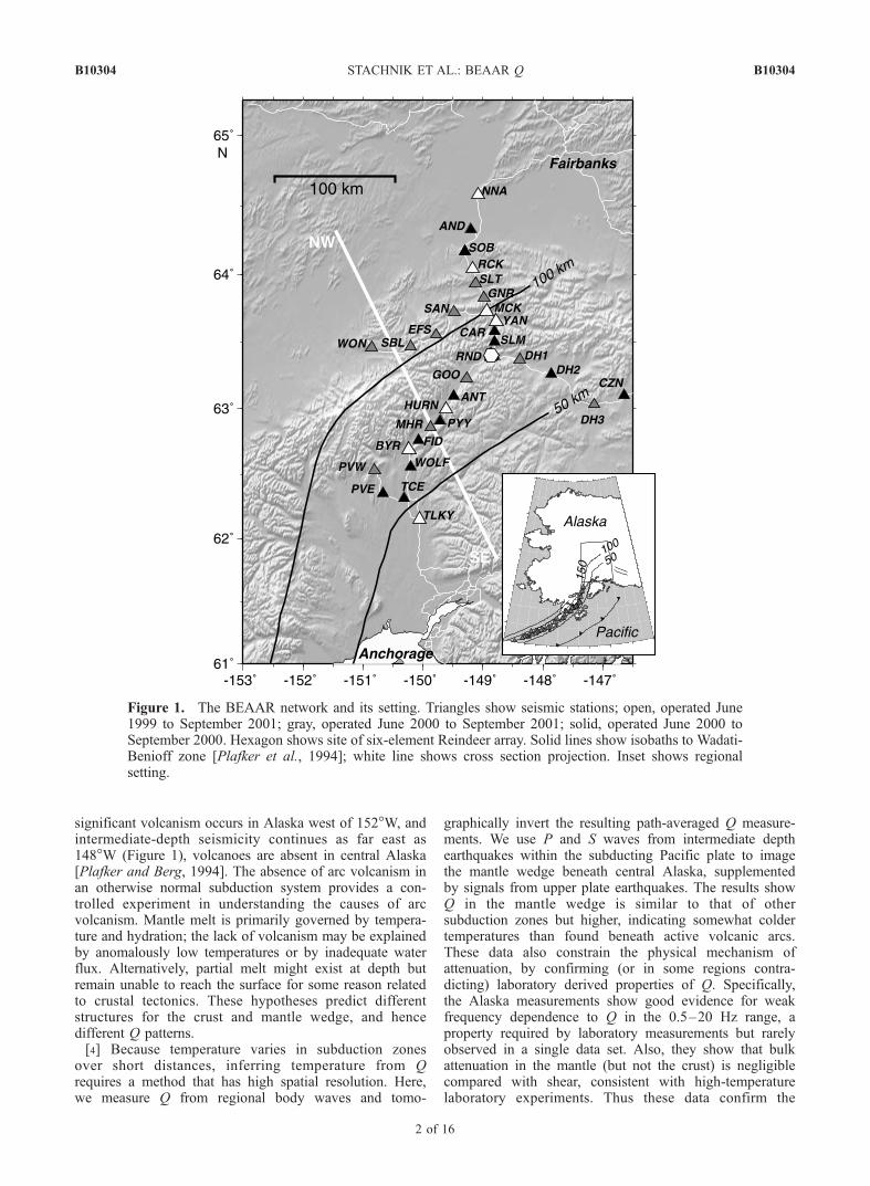
significant volcanism occurs in Alaska west of 152�W, andintermediate-depth seismicity continues as far east as148�W (Figure 1), volcanoes are absent in central Alaska[Plafker and Berg, 1994]. The absence of arc volcanism inan otherwise normal subduction system provides a con-trolled experiment in understanding the causes of arcvolcanism. Mantle melt is primarily governed by tempera-ture and hydration; the lack of volcanism may be explainedby anomalously low temperatures or by inadequate waterflux. Alternatively, partial melt might exist at depth butremain unable to reach the surface for some reason relatedto crustal tectonics. These hypotheses predict differentstructures for the crust and mantle wedge, and hencedifferent Q patterns.[4] Because temperature varies in subduction zones

over short distances, inferring temperature from Qrequires a method that has high spatial resolution. Here,we measure Q from regional body waves and tomo-

graphically invert the resulting path-averaged Q measure-ments. We use P and S waves from intermediate depthearthquakes within the subducting Pacific plate to imagethe mantle wedge beneath central Alaska, supplementedby signals from upper plate earthquakes. The results showQ in the mantle wedge is similar to that of othersubduction zones but higher, indicating somewhat coldertemperatures than found beneath active volcanic arcs.These data also constrain the physical mechanism ofattenuation, by confirming (or in some regions contra-dicting) laboratory derived properties of Q. Specifically,the Alaska measurements show good evidence for weakfrequency dependence to Q in the 0.5–20 Hz range, aproperty required by laboratory measurements but rarelyobserved in a single data set. Also, they show that bulkattenuation in the mantle (but not the crust) is negligiblecompared with shear, consistent with high-temperaturelaboratory experiments. Thus these data confirm the

Figure 1. The BEAAR network and its setting. Triangles show seismic stations; open, operated June1999 to September 2001; gray, operated June 2000 to September 2001; solid, operated June 2000 toSeptember 2000. Hexagon shows site of six-element Reindeer array. Solid lines show isobaths to Wadati-Benioff zone [Plafker et al., 1994]; white line shows cross section projection. Inset shows regionalsetting.

B10304 STACHNIK ET AL.: BEAAR Q

2 of 16

B10304

appropriateness of laboratory measurements of Q topredict temperature within the mantle wedge.

2. Attenuation Mechanisms

[5] Attenuation of seismic waves can be controlled bytemperature, water content, and cracks or porosity ofmaterials [Karato and Spetzler, 1990; Mitchell, 1995].The attenuation of P and S waves, measured here as QP

and QS, varies with attenuation of bulk and shear elasticmoduli Qk and Qm, as

1=QP ¼ 1� Rð Þ=Qkþ R=Qm ð1aÞ

1=QS ¼ 1=Qm ð1bÞ

where R = 4VS2/3VP

2, and VP, VS are the P and S velocities,respectively [Aki and Richards, 1980]. At near-solidusconditions (temperatures above 900–1000�C), laboratoryexperiments show that seismic energy is dissipated throughgrain boundary interactions [Sato et al., 1989] or intra-granular relaxation [Jackson et al., 2002, 1992; Karato andSpetzler, 1990], with 1/Qm � 1/Qk for both mechanisms.Addition of small amounts of water, as hydrogen impuritiesin olivine crystals, may have the effect of lowering Q(increasing attenuation) in a manner indistinguishable fromtemperature changes [Karato, 2003], although directmeasurements of this effect on Q have not yet been made.At temperatures substantially below solidus, it is likely thatother processes attenuate seismic waves, including inter-granular thermoelasticity and (at low pressures) deformationof cracks [e.g., Budiansky et al., 1983; Karato and Spetzler,1990; Winkler and Nur, 1979]. These latter processes canproduce substantial 1/Qk. Therefore the relationship of QP

to QS should provide some insight into the attenuationmechanism, an approach which has indicated near-solidusconditions (i.e., 1/Qm � 1/Qk) beneath the Lau back arc[Roth et al., 1999]. Some contribution from scattering toapparent attenuation may exist, particularly if 1/Q fromthese other processes is small.[6] In laboratory studies, Q is found to be dependent on

frequency [e.g., Karato and Spetzler, 1990], a property weconfirm here with seismic data. Typically, the dependence isdescribed as Q � f a for frequency f. Experiments at hightemperatures give a = 0.27 for dunite at seismic frequencies[Jackson et al., 2002], with older experiments generallyshowing a = 0.1–0.3 [Karato and Spetzler, 1990]. Thisweak frequency dependence seems generally consistentwith long-period variations in Q at mantle depths [e.g.,Warren and Shearer, 2000]. By contrast, crustal studiesshow strong frequency dependence (a > 0.5), using Lg andcoda waves (1–20 Hz) [e.g., Benz et al., 1997; McNamara,2000] or body waves in continental crust (1–25 Hz) [e.g.,Sarker and Abers, 1998a]. The physical mechanism of suchstrong frequency dependence is unclear, but probablydepends upon the presence and deformation of cracks orpores [O’Connell and Budiansky, 1977; Winkler and Nur,1979]. Although most attenuation mechanisms indicatesome frequency dependence, most measurements of Q withbody waves typically fix a = 0, usually because frequencydependence often cannot be resolved over limited frequency

ranges [e.g., Flanagan and Wiens, 1994; Schlotterbeck andAbers, 2001; Takanami et al., 2000]. In two exceptions,Flanagan and Wiens [1998] showed that a = 0.1–0.3 in theupper mantle beneath the Fiji Plateau, would reconcileseveral studies over 0.1–8 Hz, and Shito et al. [2004] founda = 0.2–0.4 in the Izu back arc from regional P wavespectra.

3. Data and Methods

3.1. Experiment

[7] From June 1999 through August 2001 we deployed theBroadband Experiment Across the Alaska Range (BEAAR),an array of 36 IRIS/PASSCAL broadband instruments acrosscentral Alaska (Figure 1). During the deployment, seveninstruments at 50 km spacing operated for the full 28 months,an additional 10 stations operated for 15 months, and all36 stations operated for 4 summer months. For this studywe analyze data only from the 4 summer months in 2000during which the entire network operated. Data derive fromRefTek 72A-08 24-bit digitizers, operating at 50 samples/s,recording signals from three-component broadband instru-ments (Guralp CMG-3T and CMG-3ESP sensors). Thisconfiguration yields a flat velocity response between fre-quencies of 0.0083 and 20 Hz, here corrected for instrumentgain and integrated to displacement. All stations had clocktimes and station locations determined by GPS.

3.2. Hypocenters and Velocities

[8] We analyze here regional earthquakes >50 km deepthat sample the slab and wedge beneath BEAAR, supple-mented with 24 events in the upper plate crust. Prelimi-nary earthquake locations are derived from monthlycatalogs produced by the Alaska Earthquake InformationCenter (AEIC) from June to September 2000 using theirautomatic detection and location system [Lindquist, 1998].These arrival times are supplemented with P and S timespicked from BEAAR records, then jointly inverted forrelocated hypocenter and one-dimensional velocity struc-ture following Roecker [1993]. The resulting data setincludes 178 hypocenters up to 140 km deep (Figures 2

Figure 2. Events used. Crosses show original cataloglocations; solid circles show relocated epicenters; trianglesshow BEAAR stations; thick gray lines show 50 and 100 kmslab isobaths; thin line shows location of cross section inFigure 3.


3 of 16

B10304

and 3), and eight-layer P and S velocity model. Mantle Pvelocities lie in the range 7.80–8.05 km/s. The relocationsreduce the scatter of the Benioff zone seismicity so thatevents depart by only a few km from a single surface, with noevents elsewhere at mantle depths. Receiver functions showthat these events all lie immediately beneath the slab surface,probably within subducted crust [Ferris et al., 2003].

3.3. Waveforms and Spectra

[9] We analyze body wave spectra of regional eventsfrom the vertical component for P waves and the transversecomponent for S waves (to minimize P-to-S mode conver-sions off horizontal discontinuities). Multitaper spectra[Park et al., 1987] are calculated from these signals inwindows 3 s in duration, beginning 0.5 s before the arrivalpick, then corrected for instrument gain and converted todisplacement. Body waves from slab events typically showshort duration, so these windows include all of the mainpulse of the waveform; signals were excluded where sig-nificant P or S energy extended past the windows. Testsshowed that increasing the window length to 4–6 s pro-duced insignificantly different spectra or attenuation mea-surements; the latter agreed with those derived for a 3 swindow with correlation coefficient of 0.93 and no signif-icant bias. The longer windows occasionally includedsecondary phases, so the 3 s windows are favored.[10] We calculate noise spectra from a 3 s long window

immediately preceding each signal window (Figure 4). ForS, the noise window consists of late P coda. The frequencyband fit varies according to signal-to-noise levels (Figure 4and Table 1), typically between 0.25 and 20 Hz, in order tomaximize information content. Low-Q paths give S wavesabove noise only at frequencies below 5–10 Hz, whilespectra from high-Q paths show little effect on amplitudesexcept at frequencies above 5–10 Hz. While a narrower

Figure 3. Cross section of hypocenters relocated usingBEAAR arrival times. Crosses show original cataloglocations; solid circles show relocated epicenters. Crosssection is located on Figure 2.

Figure 4. Spectral fitting example with S waveforms. (a) Swaves at a northern station (NNA) and (b) at a southernstation (PVW) from an event 110 km deep. D showsdistance to stations. (c) and (d) Multitaper amplitude spectraof same signals corrected to displacement (black line) or ofnoise in 3 s window immediately preceding (gray line).Thin lines show best fit model following equation (2) for aas labeled. Vertical lines show window being fit on allpanels. Note lack of high-frequency energy at NNA, typicalof wedge paths.


4 of 16

B10304

band has an advantage of consistency, a wide frequencyband is necessary to analyze wide ranges in Q. In one test,in which all spectra were limited to f < 8 Hz, QP andcrustal Q increased in variance by several times relativeto the results from all frequencies, and were essentiallyunusable. The mantle QS remained well constrained. For theupper plate events, only path lengths less than 150 km longare used in location, to avoid Pn contamination. For allevents, paths are short and generally upgoing; 50% ofsource-receiver ranges are <100 km and 90% of paths are<190 km long. Slab events range from 40 to 135 km depth.Because these ray paths are upgoing and exit the slabrapidly, three-dimensional ray bending effects should beminor throughout the wedge.[11] Of the 178 earthquakes relocated, 102 have good

signals on 6 or more stations and form the basic attenuationdata set. These earthquakes range in moment-magnitude(Mw) 2.1 to 4.7, corresponding to corner frequencies rang-ing from 2 to >20 Hz. Earthquakes are small and show awide variation in focal mechanism, so directivity effects arelikely to be minor and unsystematic.

4. Attenuation Measurements

4.1. The Parameter t** From Parametric Inversions

[12] Following common practice [e.g., Schlotterbeck andAbers, 2001], we measure path-averaged attenuation as t* =t/Q, for travel time t. A displacement spectrum recorded atstation j from earthquake k, Ajk( fi), can be approximated as[e.g., Anderson and Hough, 1984]

Ajk fið Þ ¼CjkM0k exp �pfi tjk*

� �

1þ fi=fckð Þ2ð2Þ

where fi is the ith frequency sampled, M0k and fck are theseismic moment and corner frequency, respectively, for thekth event, Cjk accounts for frequency-independent effectssuch as geometrical spreading, radiation pattern andelasticity, and t*jk is the attenuation operator. This modeldoes not include frequency-dependent site amplification andassumes a simple f 2 source spectrum, consistent with most

previous studies. We calculate Cjk from geometricalspreading, free surface and source excitation effectsconsistent with the one-dimensional velocity model, andapproximate the P and S radiation patterns by their sphericalaverage [Aki and Richards, 1980].[13] To determine the parameters, all spectra for event k

are jointly inverted for a single M0k and fck, and for separatet*jk along each path. The source parameters are determinedseparately for P and S, because the fck may differ with phase[e.g.,Madariaga, 1976]. To show the form of this inversion,equation (2) can be rewritten as a set of equations forseveral i, j:

ln Ajk fið Þ� �

þ ln 1þ fi=fckð Þ2n o

� ln Cjk

� �¼ ln M0kf g � tfi tjk*:

ð3Þ

The left-hand side of these equations contain the observeddisplacement spectra Ajk( fi) for theM stations ( j = 1, . . .,M)which record event k, corrected for source ( fck) andfrequency-independent propagation effects (Cjk). Eachspectrum is sampled continuously (at 50/512 Hz interval)at the N frequencies (i = 1, . . ., N ) for which signal-to-noiselevels are high, so N varies from record to record. For eventk, this forms a system of NM equations forM + 2 parametersln{M0k}, fck, and M values t*jk. To solve the nonlinear part ofthis problem, a sequence of values for fck is tested from 0.25to 50 Hz at 0.25 Hz intervals. At each fck the remaininglinear system of equation (3) is solved for ln{M0k} and t*jk.The fck producing the lowest misfit between left- and right-hand sides of equation (3) in the least squares sense ischosen. These measurements of t*jk are termed parametricbecause the results depend upon a parameterized descriptionof source effects.[14] The standard errors calculated from the linear part of

the problem become the formal uncertainties in the resultingt*jk used for subsequent tomographic inversions. Such uncer-tainties account for noise in observations but neglect trade-off with uncertainty in fck, which is fixed in the linearinversion. They also implicitly assume that each A( fi) areindependent, which is unlikely for windowed multitaper

Table 1. Path-Averaged Q Estimates

Path Phase Qo Errora, % Qav Error,a % Number of Data nVarb Qav-corc Error,a % fmin,

d Hz fmax,d Hz

a = 0.27Crust P 291 10 242 5.0 446 0.33 0.4 19.2Wedge P 764 66 257 4.5 340 0.41 266 19 0.8 19.1Slab P 1e - 793 10.3 515 0.87 1e - 1.0 19.2Crust S 3445 82 317 5.7 398 0.28 0.3 13.9Wedge S 174 12 173 2.4 286 0.13 138 7.7 0.3 9.4Slab S 4308 136 497 4.1 503 0.47 724 53 0.4 16.9

a = 0.0Wedge P 1696 63 528 4.0 340 0.37 537 36 0.8 19.1Wedge S 252 11 348 3.0 286 0.17 283 20 0.4 9.4

a = 0.65Wedge P 1213 328 93 5.0 340 0.45 104 6.6 0.9 19.1Wedge S 94 15 73 2.5 286 0.13 62 2.6 0.4 9.4

aFormal uncertainty (1s) in 1/Q is from regression for 1/Qo or 1/Qav, expressed as percent.bVariance of misfit to t* data is for the Qo regression, normalized to variance in t* measurements.cQav is corrected for attenuation in the crust.dThe fmin and fmax are mean minimum and maximum frequency bounds in t* measurements.eThe 1/Q estimate is negative, but uncertainties include zero.


5 of 16

B10304

spectra, so underestimate actual errors. An approximation,discussed below, accounts for these additional sources oferror in the tomographic inversion by treating them as errorsin theory [Tarantola and Valette, 1982].[15] A correction is made to account for frequency-

dependent site effects. The residual spectra (differencebetween left- and right-hand sides of equation (3)) for eachstation are averaged over all events, smoothed, and sub-tracted from the observed spectra. Then, the entire inversionprocedure is repeated, to derive final t*jk estimates. Also,three stations showing large site effects (DH1, MHR, TCE)were not used to determine fc. Results for S show littlesensitivity to site corrections, although the P results in theupper plate crust show some differences. Finally, only thosesignals showing signal-to-noise ratios above 2.5 for both Sand P were kept, so that the data set has matching S and Pobservations.[16] These procedures and subsequent outlier removal

produce a total of 2318 t*S measurements and 2066 t*Pmeasurements, used for path-averaged estimates. Of these,2004 had common station-event pairs for P and S, and wereused in tomographic inversion. For a = 0 (see below),median t* is 0.0247 s for P and 0.0474 s for S, but both varyby an order of magnitude with median formal errors of0.0016 s and 0.0024 s, respectively. The fc for P systemat-ically exceeds those for S by a factor of 1.5, consistent witha variety of source models [Madariaga, 1976]. Seismicmoments for S and P correlate well (correlation coefficient =0.93 with no significant bias), and correlate well withcatalog magnitudes [Stachnik, 2002]. Thus the inversionsrecover reasonable source parameters.

4.2. Potential Distortion of Spectra

[17] The presence of a low-velocity layer atop the sub-ducting slab, possibly representing subducted oceanic crust,has been shown to exist under central Alaska [Abers andSarker, 1996; Ferris et al., 2003]. Because such a layer actsas a frequency-dependent waveguide, the observed spec-trum for certain paths could be modeled incorrectly. Awaveguide enhances high frequencies, so should decreasethe apparent attenuation. We exclude signals that exhibitobvious dispersion by visual inspection, and exclude raypaths with long segments along the top of the slab. Still,some measurements of small (or negative) t* may beinfluenced by focusing, particularly along the slab. Theunusual parts of the slab we observe have high not lowattenuation, so cannot be explained by this mechanism.[18] Errors in fc may trade off with t*, as both parameters

affect spectral falloff [Anderson, 1986]. Several resultssuggest that this trade-off does not produce significantbiases here in source parameters, and by inference in t*.First, our fc estimates appear reasonable; they give stressdrops comparable with those elsewhere (e.g., 1–10 MPa)and are similar for P and S [Stachnik, 2002]. Second, theseismic moments estimated here are consistent with thosederived from ML magnitudes for Alaska earthquakes aftercorrecting for known path biases [Lindquist, 1998; Stachnik,2002]. Third, in several tests we reinverted all spectra withdifferent assumptions about the source, and the resultingattenuation estimates show no systematic changes. Thesetests include (1) fc fixed a priori from the earthquakemagnitude and assumed stress drop (10 MPa); (2) fc

arbitrarily set to 40 Hz, well outside the range of fits;(3) earthquakes restricted to those with M < 2.2, a size forwhich corner frequencies should significantly exceed therange of frequencies sampled (see section 4.4); and (4) asource model with sharper corner, in which the denominatorin equation (2) is changed to [1 + ( f/fc)

4]1/2 [Abercrombie,1995]. In all of these tests, the resulting changes toattenuation lie inside the calculated uncertainties. Overall,while errors in source parameterization may contribute touncertainties, they do not seem to significantly bias theestimated attenuation.

4.3. Q From S-to-P Spectral Ratio

[19] As a check on the parametric measurement of t*(equation (3)), we also estimate Q from the spectral ratio ofS to P waves, an approach which should approximatelyremove source, site and instrument effects [e.g., Roth et al.,1999]. The method gives estimates of dt* = t*S � t*P, whichrequire assumptions about QP/QS to interpret, a quantitywhich we find varies greatly. The overall pattern of atten-uation inferred from dt* resembles that from t*S, and givessimilar estimates of QS for highly attenuating wedge paths;the similarity can be seen by comparing dt* to parametricestimates of t*S � t*P (Figure 5). Uncertainties are similarfor the two techniques; suites of dt* measurements fromevent clusters to individual stations show statistical variancethat is comparable to that of parametric t*S or t*P. Thissimilarity in variance may indicate that trade-offs betweent*S and fc, presumably eliminated in dt*, are not a majorsource of error. A small bias between dt* and t*S � t*P mayresult from the assumption that fc is the same in P and S inthe ratio technique. Also, at high t*, the t*P appears slightlyunderestimated. A positivity constraint applied to tomogra-phy (see below) removes this slight shift. Because no majorbiases could be found between the two sets of results, and

Figure 5. Comparison of dt* to parametric estimates oft*S � t*P. Each symbol represents average measurement forone station over events in one depth range (symbol). Dashedline shows 1:1 relationship, gray line shows estimated biasin dt* if P and S corner frequencies differ by a factor of 1.5,as expected [Madariaga, 1976]. Similarity of two axesindicates that the parametric method accounts for sourceeffects adequately.


6 of 16

B10304

interpretation of dt* requires assumptions about QP/QS, wedo not discuss these results further.

4.4. Frequency Dependence

4.4.1. Estimation of A[20] Physical mechanisms of attenuation can be poten-

tially discriminated by their frequency dependence, de-scribed by

t* ¼ to*f�a ð4Þ

where t*o represents attenuation at 1 Hz. We constrainthis frequency dependence substituting equation (4) intoequations (2) and (3), then invert each spectra for t*o in themanner described above, but with a fixed at values from 0.0to 1.0 at 0.1 increments. The a is estimated by minimizingthe global variance of the misfit for large data subsets(Figure 6). For simplicity, t*o is referred to as t* insubsequent discussions.[21] We estimate a for the entire data set and for three

subsets: (1) paths that sample upper plate crust (pathsfrom sources <40 km deep); (2) mantle wedge paths(sources >85 km deep, north of 63�N, west of 149�W, tostations north or west of MCK), and (3) slab paths (sameevents as wedge, but to stations south or east of RND).For the entire data set, a = 0.7 or 0.6 fit P or S best,respectively, and similar values are found for crustalpaths (Figure 6). The independent estimate of a = 0.66at 1–20 Hz from crustal Lg phases in central Alaska[McNamara, 2000] agrees closely, indicating that thefrequency dependence is robust and well constrained,

and that similar processes likely attenuate both body wavesand Lg. Values of a near 0.65 typify many tectonicallyactive areas [Mitchell, 1995].[22] By comparison, both wedge and mantle paths

show significantly lower values of a, near 0.4–0.5 inthe wedge and slightly higher for slab paths (Figure 6).These mantle paths sample the crust for roughly one thirdof their length, for which a = 0.6–0.7. Hence attenuationin the mantle must then exhibit somewhat less frequencydependence than a = 0.4–0.5, likely close to the a = 0.27indicated by high-temperature laboratory experiments[Jackson et al., 2002; Karato, 2003]. In the wedge theseexperiments should have most relevance, so it is reassur-ing that the observed frequency dependence agrees withthat predicted for high-temperature mantle rock. Flanaganand Wiens [1998] and Shito et al. [2004] observe similara for back arc paths.[23] It is possible that the inferred frequency depen-

dence represents some bias in the fitting procedure, ratherthan real frequency dependence, but several tests suggestotherwise. Increasing a decreases the rate at whichamplitudes decay with increasing frequency, an effectwhich may be mimicked by errors in the description ofthe source spectra. To test this effect, we recalculated ausing only the 33% of the data set corresponding to smallevents (ML < 2.2), which should have corner frequenciesabove the frequency band being studied. The results shownearly identical minima in variance of misfit with a,indicating that a source parameterization error is notproducing apparent frequency dependence. In two relatedtests, we fixed fc to an arbitrary high value, and to avalue predicted from the local magnitude assuming con-stant stress drop. The results show greater scatter, but nosystematic change in a.4.4.2. Implications for Comparing Q From DifferentStudies[24] Attenuation estimates at 1 Hz (from t*o) vary system-

atically with a, such that larger a gives lower Q at 1 Hz(Figure 7 and Table 1). Estimates of Q at different a

Figure 6. Variance of misfit to spectra summed over dataset, as a function of frequency dependence parameter a,normalized to minimum variance value for phases shown.Np and Ns give number of records used for P and S,respectively.

Figure 7. Variations in path-averaged Q with frequencyfor the mantle wedge (Qav, Table 1) for varying a. S waves(thick lines) all give similar Q near fR = 10 Hz for any a,while P waves (thin lines) give same values near fR = 15 Hz.The maximum frequencies sampled ( fmax, Table 1) lie nearfR, indicating that the greatest sensitivity to Q lies at thehighest frequencies used.


7 of 16

B10304

converge above 1 Hz, such that the estimates for all aconverge at a common frequency, fR, for any given datasubset. The common frequency fR lies at the high end ofthe frequency band sampled, near 10–20 Hz dependingupon path ( fmax in Table 1), a pattern which indicates thatthese measurements are most sensitive to attenuation nearfmax. This seems reasonable, as the amplitude reductionof spectra relative to a nonattenuating signal should begreatest at highest frequencies. In other words, any similarmeasurements of Q, particularly those assuming no fre-quency dependence, mostly reflect Q at the upper end ofthe frequency band sampled. We suspect this is true ofany measurement of attenuation based upon spectralfalloff [e.g., Haberland and Rietbrock, 2001; Roth et al.,1999; Tsumura et al., 2000]. Some of the variationbetween studies may just reflect this difference in samplefrequencies, and the frequency dependence of Q. Thusspectra-based measurements of Q cannot be comparedwithout knowing something about the frequency band ofmeasurement.[25] One consequence of this phenomenon is that fre-

quency-independent estimates will tend to systematicallyoverestimate Q (underestimate attenuation) at frequenciesbelow fR. Applications of such Q estimates, for example inpredicting seismic hazards, should take this effect intoaccount.4.4.3. Comparing Results for Different A[26] Both path-averaged Q measurements and tomo-

graphic estimates show similar patterns for all assumed a,so results for one value of a should be predictable fromanother. Rather than present results for all a in detail, wepresent results for a = 0.27 only, a value most appropriatefor the mantle wedge. Results for other a can be derived asfollows. Figure 7 shows that at some frequency, fR, the t*estimates for all a will agree. Then

Q1 að Þ ¼ Q1 0ð Þ fR=1 Hzð Þ�a ð5Þ

where Q1(a) represents a path-averaged Q estimate at 1 Hzfor a given a, and Q1(0) is the frequency-independentestimate. This relationship best fits the entire data set forfR = 13 Hz; however, fR varies with Q. The signal-to-noiseratio at high frequencies decreases with decreasing Q(greater spectral falloff), so fR decreases with decreasing Q,approximately as

fR ¼ aQ1 0ð Þk ð6Þ

for constants a and k. Regression of S wave t* measure-ments gives k = 0.505 ± 0.012 and ln(a) = �0.64 ± .08, forfR in Hz (1s uncertainties). This relationship can explain90.5% of the variance in Q1(a > 0) relative to Q1(0).

4.5. Path-Averaged Q

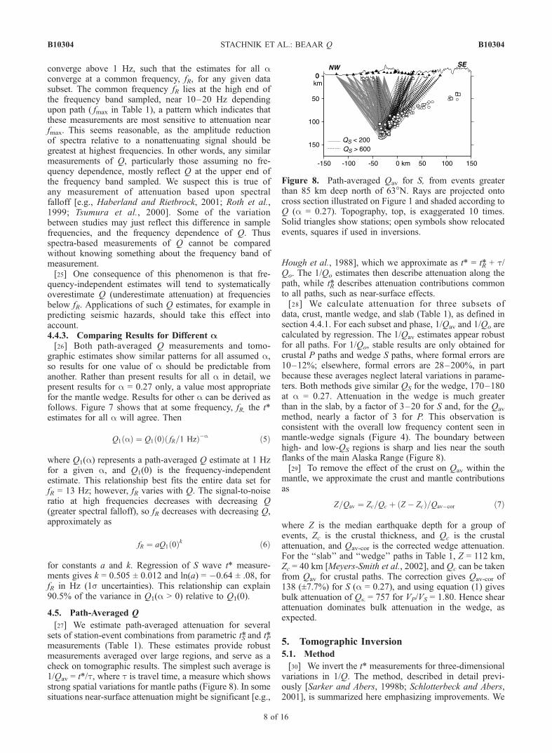
[27] We estimate path-averaged attenuation for severalsets of station-event combinations from parametric t*S and t*Pmeasurements (Table 1). These estimates provide robustmeasurements averaged over large regions, and serve as acheck on tomographic results. The simplest such average is1/Qav = t*/t, where t is travel time, a measure which showsstrong spatial variations for mantle paths (Figure 8). In somesituations near-surface attenuation might be significant [e.g.,

Hough et al., 1988], which we approximate as t* = t*R + t/Qo. The 1/Qo estimates then describe attenuation along thepath, while t*R describes attenuation contributions commonto all paths, such as near-surface effects.[28] We calculate attenuation for three subsets of

data, crust, mantle wedge, and slab (Table 1), as defined insection 4.4.1. For each subset and phase, 1/Qav and 1/Qo arecalculated by regression. The 1/Qav estimates appear robustfor all paths. For 1/Qo, stable results are only obtained forcrustal P paths and wedge S paths, where formal errors are10–12%; elsewhere, formal errors are 28–200%, in partbecause these averages neglect lateral variations in parame-ters. Both methods give similar QS for the wedge, 170–180at a = 0.27. Attenuation in the wedge is much greaterthan in the slab, by a factor of 3–20 for S and, for the Qav

method, nearly a factor of 3 for P. This observation isconsistent with the overall low frequency content seen inmantle-wedge signals (Figure 4). The boundary betweenhigh- and low-QS regions is sharp and lies near the southflanks of the main Alaska Range (Figure 8).[29] To remove the effect of the crust on Qav within the

mantle, we approximate the crust and mantle contributionsas

Z=Qav ¼ Zc=Qc þ Z � Zcð Þ=Qav�cor ð7Þ

where Z is the median earthquake depth for a group ofevents, Zc is the crustal thickness, and Qc is the crustalattenuation, and Qav-cor is the corrected wedge attenuation.For the ‘‘slab’’ and ‘‘wedge’’ paths in Table 1, Z = 112 km,Zc = 40 km [Meyers-Smith et al., 2002], and Qc can be takenfrom Qav for crustal paths. The correction gives Qav-cor of138 (±7.7%) for S (a = 0.27), and using equation (1) givesbulk attenuation of Qk = 757 for VP/VS = 1.80. Hence shearattenuation dominates bulk attenuation in the wedge, asexpected.

5. Tomographic Inversion

5.1. Method

[30] We invert the t* measurements for three-dimensionalvariations in 1/Q. The method, described in detail previ-ously [Sarker and Abers, 1998b; Schlotterbeck and Abers,2001], is summarized here emphasizing improvements. We

Figure 8. Path-averaged Qav for S, from events greaterthan 85 km deep north of 63�N. Rays are projected ontocross section illustrated on Figure 1 and shaded according toQ (a = 0.27). Topography, top, is exaggerated 10 times.Solid triangles show stations; open symbols show relocatedevents, squares if used in inversions.


8 of 16

B10304

approximate heterogeneity by blocks of constant velocity Vand 1/Q. Then t* for the ith ray path is

ti* ¼Xj

lij=VjQj ð8Þ

where lij is the path length of the ith ray in the jth block andVj and 1/Qj are the velocity and attenuation parameter,respectively, of block j. To the extent that V can beconstrained independently of 1/Q, a linear relationship thenexists between 1/Qj and t*i, that can be inverted. (Physicaldispersion introduces some coupling [Karato, 1993], butthe effects of these velocity variations on t* are negligible.)For simplicity, rays are traced in a one-dimensional velocitymodel.[31] The inversion of the t*i for 1/Qj follows the

maximum-likelihood linear inverse theory of Tarantolaand Valette [1982]. In the absence of observations, resultsare constrained to an a priori model PREM [Dziewonski andAnderson, 1981], modified to include a lossy near-surfacelayer (QS = 50 in the upper 500 m). The a priori modeluncertainties are set to 100% in 1/Q, and we do not includeany smoothness constraints other than finite block size, asthe data are well behaved. Uncertainties in observations areassumed to be those determined from the t* measurements,treated as Gaussian. To account for unmodeled errors in thet* measurements (see section 4.1), the inversion includesan a priori uncertainty in theory sT, which quantifies errorsin the theoretical relationships used to predict observations[Tarantola, 1987]. The sT incorporates errors due to finiteblock size, to errors in fc and the source model generally,and to other approximations in the theory used to predict1/Q. We set sT = 0.03 s for all observations being fit,derived from the measured variation in t* over collocatedclusters of events (for details, see Stachnik [2002]).[32] Initial inversions showed that, for a few poorly

resolved blocks, 1/QP < 0.41/QS, giving the nonphysicalresult that 1/Qk < 0 (equation (1), for VP/VS = 1.80 as inPREM). However, larger 1/QP could fit the data nearlyequally well. To enforce the physical constraint that 1/Qk� 0,the final inversions for 1/QP include an iterative stepwhich adjusts those nodes which 1/QP < 0.41/QS, bysimultaneously increasing their damping and reducing theira priori 1/QP toward 0.41/QS. No more than threeiterations are necessary in most cases to enforce the 1/Qk � 0 constraint for all but one or two nodes. Theresulting models have the benefit that 1/Qk everywhere isnonnegative, and that trade-offs between damped andundamped blocks are handled correctly. This procedureincreases global variance of misfit in P by only 4.8%relative to inversions with no positivity constraints, lessthan the variance change associated with minor changes togrid geometry. We use 1/QPu to denote P results fromthe unconstrained inversion, and 1/QPc to denote inver-sions for which 1/Qk is constrained to be positive. Asimilar process enforces 1/QS > 0 for all blocks, althoughalmost no well-resolved nodes are affected.

5.2. Inversion Parameterization

[33] We take two approaches to parameterization, oneemphasizing resolution of small features, and another‘‘minimum parameterization’’ method designed to recover

1/Q averages with high accuracy. The first follows thestandard approach of dividing the earth into small cells ofconstant 1/Q, and inverting for them. A top layer accountsfor near-surface effects, extending beneath each station to500 m below sea level, with 10 km horizontal grid spacingso that each station lies on a separate block. Such a layerallows expected high near-surface attenuation [e.g., Houghet al., 1988]. Below this layer, the inversion grid is brokeninto regular cells in both crust and mantle, 20 km wideacross strike but much longer along strike (Figure 9).Horizontal boundaries include a Moho at 40 km depth, asindicated by receiver functions [Ferris et al., 2003; Meyers-Smith et al., 2002], and others at 20 km intervals. Asequence of across-strike block widths was tested, forspacings of 10–50 km, and 20 km was the smallest sizeto significantly reduce variance over larger blocks. Weexpress results as 1000/Q, for convenience.

5.3. Inversion Results

5.3.1. Overview[34] Inversions show high 1000/QS (high attenuation) in

the mantle wedge and generally low 1000/QS in bothupper plate crust and downgoing slab (Figure 10). The high1000/QS wedge exists only where the slab is deeper than80 km, and shows an abrupt termination to the SE wherethe slab shallows. The highest attenuation in the wedge has1000/QS = 7–10 (QS = 100–140) for a = 0.27, withstandard errors near 1.0, in accord with path-averagedestimates (Table 1). This high attenuation dominates thesignals (e.g., Figures 4a and 4c). The upper plate crustshows 1000/QS < 2.5, and the slab below 75 km depthshows even less attenuation (1000/QS < 1.0). Unexpectedly,the slab shows relatively high attenuation at depths less than80 km, 1000/QS = 2.5–5.5. This region appears to be wellresolved and can be recovered from inversions of smallsubsets of the data with limited ranges of path length.[35] The P results differ substantially from S. Crust

shows high attenuation, while the mantle wedge showslittle. The QPu image has a region of almost no attenu-ation immediately above the slab at 50–100 km depth, a

Figure 9. Grid used for 1/Q inversions, showing constantQ blocks, for all depths except the near-surface. Trianglesshow stations; thick gray lines show 50 and 100 km slabisobaths.


9 of 16

B10304

feature which becomes less pronounced in QPc. Still,1000/Qk is generally low in the mantle (<1.0) and 2–5 times higher in the crust. Both 1000/QS and 1000/Qk showthe high-attenuation region within the slab at <80 km depth,discussed below.[36] Crustal attenuation lies in the range 1000/QS = 1–3,

averaging 1.3. McNamara [2000] found QS = 220 from Lgcoda at 1 Hz, and a = 0.66, equivalent to 1000/QS = 1.4 ata = 0.27 following equations (5) and (6), consistent withthe measurements here. Our 1000/QP is somewhat higher,giving 1000/Qk � 5–7 directly beneath the northernmoststations. The high 1000/Qk may reflect unusual basineffects, as these stations lie on the Central Tenana Basinsediments, 2 km thick including up to 1 km of Pliocenegravels [Kirschner, 1994]. High P wave attenuation typifiesmany crustal studies in tectonically active areas [e.g.,Mitchell, 1995; Rautian et al., 1978; Schlotterbeck andAbers, 2001], probably a combination of poroelastic andscattering effects.[37] Attenuation for the near-surface layer, representing

site effects, ranges from 1000/Q = 10–120, with medians of28 and 35 for P and S, respectively. These values are an orderof magnitude greater than 1000/Q for the blocks immediatelybelow, consistent with the a priori assumptions and withestimates for weathered layers elsewhere [Abercrombie,1997; Aster and Shearer, 1991].5.3.2. Formal Resolution and Uncertainty[38] For both 1000/QPu and 1000/QS, blocks near the

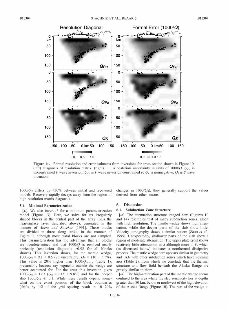
surface layer show high resolution (resolution matrix diag-onals >0.9), as do those in the mantle wedge (40–100 kmdepth) and the crust directly beneath the array (Figure 11).

Lower resolution diagonals are observed for the subductinglithosphere below the earthquakes (<0.7) and in the north-ernmost part of the mantle wedge (<0.5, all depths). Thispattern reflects ray coverage. Rays sample the mantle wedgeby short and crossing paths between the intermediate-depthearthquakes and the stations, but sample the downgoingplate only by long along-strike paths and just near its uppersurface. 1000/QPc shows a similar pattern except below80 km depth, where the positivity constraint dominates andresolution is low. Formal errors show a pattern similar toresolution, modified by variations of a priori constraints, asexpected [Jackson, 1979].5.3.3. Numerical Resolution Tests[39] Numerical tests also demonstrate the recovery of

features. In each, we trace the ray paths for all station-eventpairs through a simple 1000/Q model to generate syntheticdata, with structure resembling features of interest, and theninvert these predicted t* values in the same manner as realdata, to recover the simple model. We discuss QS results; QP

is similar.[40] A checkerboard test (Figure 12a) shows that fea-

tures of 20 km dimension can be resolved through muchof the wedge, in the volume between the slab seismicityand the stations. Amplitude recovery in the northern partof the wedge is roughly 80% beneath the stations, fallingoff rapidly to the north. Structure below the seismic zoneshows relatively poorer recovery. The high-attenuationregion of the slab <80 km deep appears to be wellresolved.[41] A second test (Figure 12b) simulates the effect of a

high-attenuation mantle wedge. Where resolution is high,

Figure 10. Results of tomographic inversion in cross section (Figure 1): (a) 1000/QS, (b) 1000/QP withno constraints, (c) 1000/QP constrained so that 1000/Qk is nonnegative, and (d) resulting bulk modulusattenuation 1000/Qk, from equation (1). Circles show events; triangles show stations projected onto crosssection. Elevations and topography are exaggerated 10 times. White corresponds to a priori model, 1000/Q = 1.67 (Q = 600). See color version of this figure at back of this issue.


10 of 16

B10304

1000/QS differs by <30% between initial and recoveredmodels. Recovery rapidly decays away from the region ofhigh-resolution matrix diagonals.

5.4. Minimal Parameterization

[42] We also invert t* for a minimum parameterizationmodel (Figure 13). Here, we solve for six irregularlyshaped blocks in the central part of the array (plus thenear-surface layer described above), generated in themanner of Abers and Roecker [1991]. These blocksare divided in three along strike, in the manner ofFigure 9, although most distal blocks are not sampled.This parameterization has the advantage that all blocksare overdetermined and that 1000/Q is resolved nearlyperfectly (resolution diagonals >0.98 for all blocksshown). This inversion shows, for the mantle wedge,1000/QS = 9.1 ± 0.5 (2s uncertainty; QS = 110 ± 5.5%).This value is 20% higher than 1000/Qav-cor (Table 1),presumably because ray segments outside the wedge arebetter accounted for. For the crust this inversion gives1000/QS = 1.63 (QS = 613 ± 9.8%) and for the deeperslab 1000/QS � 0.1. While these results depend some-what on the exact position of the block boundaries(shifts by 1/2 of the grid spacing result in 10–20%

changes in 1000/QS), they generally support the valuesderived from other means.

6. Discussion

6.1. Subduction Zone Structure

[43] The attenuation structure imaged here (Figures 10and 14) resembles that of many subduction zones, albeitwith high resolution. The mantle wedge shows high atten-uation, while the deeper parts of the slab show little.Velocity tomography shows a similar pattern [Zhao et al.,1995]. Unexpectedly, shallower parts of the slab show aregion of moderate attenuation. The upper plate crust showsrelatively little attenuation in S although more in P, which(as discussed below) indicates a nonthermal dissipativeprocess. The mantle wedge here appears similar in geometryand 1/QS with other subduction zones which have volcanicarcs (Table 2), from which we conclude that the thermalstructure and flow field beneath the Alaska Range aregrossly similar to them.[44] The high-attenuation part of the mantle wedge seems

confined to the area where the slab seismicity lies at depthsgreater than 80 km, below or northwest of the high elevationof the Alaska Range (Figure 10). The part of the wedge to

Figure 11. Formal resolution and error estimates from inversions for cross section shown in Figure 10.(left) Diagonals of resolution matrix. (right) Full a posteriori uncertainty in units of 1000/Q. QPu isunconstrained P wave inversion; QPc is P wave inversion constrained so Qk is nonnegative; QS is S waveinversion.


11 of 16

B10304

the southeast, where the slab is shallower, shows moderateto high 1/Q. A similar pattern has been observed in northernJapan [Takanami et al., 2000] and likely typifies manysubduction zones. The simplest explanation is that the low-Qzone represents hot flowing mantle, while the high-Qmantle is a cold, viscous nose of the wedge that is isolatedfrom large-scale flow, consistent with numerical experi-ments [Kincaid and Sacks, 1997]. Partial serpentinizationof this cold, shallow part of the wedge would increase itsbuoyancy and further increase its resistance to flow. Theboundary between high- and low-Q wedges also corre-sponds with a 90� rotation in mantle anisotropy inferred

from shear wave splitting [Christensen et al., 2003], sup-porting the inference that marks a boundary between flowregimes. The boundary lies along the southern margin of theAlaska Range, a major mountain belt actively forming wellinland of the subduction zone. Perhaps, the contrast instrength between hot and cold mantle, inferred from atten-uation, provides a control on localization of strain here.

Figure 12. Numerical resolution tests. (a) Checkerboard resolution test. Starting checkerboard has20 km blocks in two dimensions, with 1000/Q alternating between the a priori value, 1.7, and 10. Notegood recovery throughout region. (b) High-attenuation mantle wedge test. Attenuation measurementsgenerated 1000/Q = 10 in wedge, bound by white line, and 1.7 elsewhere. Both tests use same raysand uncertainties as actual QS result. Circles show events; triangles show stations. Blocks labeled with1000/Q if resolution diagonals exceed 0.01 (only within wedge for Figure 12b). This is same crosssection as Figure 10. For well-resolved blocks, amplitude recovery is 69–87%.

Figure 13. Minimum parameter inversion for 1000/QS.Format is the same as Figure 10. Formal errors are 2s.

Figure 14. Cartoon illustrating main Q regimes. DF showsDenali Fault trace.


12 of 16

B10304

Regardless, a prominent lateral boundary divides the wedgebetween a shallow, presumably cold region to the south, andthe hot region that comprises most of its volume.[45] All inversions show a well-resolved region of high

attenuation within the slab, where slab seismicity lies atshallow depths of 40–80 km. This part of the subductingplate has been shown from receiver functions to consist of athick low-velocity layer, 14–22 km wide, probably crust ofa subducting exotic terrane that has not converted toeclogite [Ferris et al., 2003]. Over the 40–80 km depthrange the seismic velocities within the layer increase sig-nificantly with increasing depth, perhaps indicating that theoceanic crust is dehydrating. The breakdown of hydrousminerals in subducted crust introduces free H2O to theregion, which could significantly affect shear and perhapsbulk moduli, depending upon crack geometry and density[e.g., Schmeling, 1985; Takei, 2002]. The imaged high-attenuation region corresponds closely to the subductedcrust.

6.2. QK-QM Relationship and Physical Mechanism

[46] Four distinct regimes can be defined on the basisof 1/Qk and 1/QS (1/Qm): (1) a hot mantle wedge, with high1/Qm and near-zero 1/Qk; (2) a cold slab >80 km deep withgenerally low attenuation; (3) an upper crust with low butvariable 1/Qm and moderate 1/Qk; and (4) an unusualportion of the slab <80 km deep with moderate to high 1/Qmand 1/Qk. The (1/Qk)/(1/Qm) ratio (Figure 15) shows strongchanges across the Moho of the upper plate, and at the topof the downgoing plate as inferred from seismicity. In theintervening mantle wedge, 1/Qk � 1/Qm, while in both thedowngoing and overlying crust, 1/Qk is relatively signifi-cant. These variations are unlikely to be due to varyingresolution because the P and S inversions use exactly thesame ray paths for identical sets of source-receiver pairs.[47] The mantle wedge exhibits high 1/Qm, negligible

1/Qk, and frequency dependence consistent with a = 0.27.These observations validate the application here ofthermally activated, high-temperature background attenua-tion models derived from laboratory data [Jackson et al.,2002; Karato, 2003]. While these mechanisms are oftenassumed to be applicable [Nakajima and Hasegawa, 2003],such supporting observations are rarely available. Bycontrast, no such theory can be applied to the other regionswhere 1/Qk is significant, and interpretation is necessarily

qualitative. For example, the shallow portion of the slabmay have elevated 1/Qk and 1/Qm because fluids areabundant, as discussed above, but it is difficult to constrainthe fluid content or pore geometry needed to produce theobservations.[48] In both the upper plate crust and descending crust

1/Qk is significant, indicating that some other mechanismmust be attenuating seismic waves. Possibly scattering mayplay a role. However, the QS for the crust inferred here issimilar in both value and a to that inferred from Lg andfrom coda [McNamara, 2000], despite the differences inhow these wave types sample the scattered wave field. Thissimilarity indicates intrinsic effects dominate Q [Sarker andAbers, 1998a]. As discussed above, poorly consolidatedbasin sediments may affect parts of the crustal signal, asmight an abundance of fractures or fluid circulation intectonically active regions.[49] In the slab and perhaps crust, it is possible that

heterogeneous materials exhibit significant thermoelasticity,a mechanism that should affect 1/Qk strongly [Budianskyet al., 1983; Heinz et al., 1982]. Although this mechanismis not thought to be important most places in the Earth, incold slabs the normal thermal mechanisms affecting Qmshould be unimportant, so other processes may dominate. Inheterogeneous materials, thermoelastic attenuation derives

Table 2. Q Measurements in Centers of Mantle Wedges, 50–100 km Depth

Region QP QS Band,a Hz a Reference

Central Alaska 537 ± 193 283 ± 57 0.3–9(S), 1–19(P) 0 this studyCentral Alaska 266 ± 51 138 ± 11 0.3–9(S), 1–19(P) 0.27 this studyCentral Alaska - 141b ± 25 0.3–9(S), 1–19(P) 0 this study, from dt*Central Alaska 205–345 95–140 0.3–9(S), 1–19(P) 0.27 this study, tomographyCentral Alaska 218 ± 10 110 ± 6 0.3–9(S), 1–19(P) 0.27 this study, minimum parameterNE Japan 150 - 1.0–20?c 0 Tsumura et al. [2000]NE Japan - 70–120b 1.0–8.0 0 Takanami et al. [2000]Andes 300 100 0.8–5 0 Myers et al. [1998]Andes 80–150 - 1 to (7–30) 0 Schurr et al. [2003]Tonga (Lau Basin) 240 - 1.0–7.6 0 Bowman [1988]Tonga (Lau Basin) 120–121 45–57 0.05–0.5 0.1–0.3 Flanagan and Wiens [1998]Tonga (Lau Basin) 90b - 0.1–3.5 0 Roth et al. [1999]

aCharacteristic frequency band sampled; numerical experiments indicate that Q is measured at the upper end of this band.bBased on S-to-P spectral ratios.cEstimated from figures of Tsumura et al. [2000].

Figure 15. Attenuation ratio for bulk modulus to shearmodulus from division of images in Figure 10. In mantlewedge, bulk modulus attenuation is negligible, while it issignificant in the crust and descending plate. See colorversion of this figure at back of this issue.


13 of 16

B10304

from differences in compressibility and thermal conductiv-ity between components in polycrystalline aggregates.Although anhydrous mantle is predicted to have Qk �5000 from this process [Heinz et al., 1982], the process isnot well understood. The presence of hydrous phases andisolated free fluid pockets could greatly enhance the grain-scale heterogeneity of subducting slabs, which in turn couldincrease 1/Qk through this effect. These mechanisms shouldhave frequency dependence of a = 0.5 [Budiansky et al.,1983], consistent with slab paths here (Figure 6).

6.3. Inferred Temperature and Comparison WithOther Arcs

[50] In the mantle wedge, the BEAAR data indicate QS �100–150 at 1 Hz for a = 0.27 (Table 1 and Figures 10 and13). To compare these results with those from other studies,which commonly assume a = 0, our Q estimates for thewedge should be multiplied by 2.0 (QS = 125 gives fR =10 Hz; see section 4.4.3). The conversion depends upon themaximum frequency (fR) used to measure Q, which likelyvaries from study to study, so values are not directlycomparable unless fR is similar. Still, compared with otherarcs, the wedge beneath Alaska appears to be less attenu-ating (Table 2 and Figure 16).[51] To estimate temperature (T), we assume that the

high-T background model for Q applies to the wedge, asmeasured by the laboratory experiments of Jackson et al.[2002], and that H2O content or grain size variations can beignored. Temperatures are calculated at a depth of 80 km

(2.45 GPa), assuming an activation volume of 13.8 cm3/molderived from comparing Q to T globally [Abers et al.,2003]. This pressure correction increases T estimates by130�C from laboratory values (at 0 GPa), and lies within therange of laboratory estimates for activation volume [Hirthand Kohlstedt, 2003]. For a nominal grain size of 1 mm, theAlaska results indicate T � 1250�C with 25–50� uncertain-ties, both from the a = 0.27 results at 1 Hz and from thea = 0 results at 10 Hz. Changes in grain size, activationvolume, or water content would change these absoluteestimates, typically on the order of 100�C, but the relativevariations in T do not change much. Results from otherwedges, compared at the highest frequency sampled, showT to be 100�C higher for the Andes and NE Japan, stillbelow the dry solidus of 1420�C at 2.45 GPa [Hirschmann,2000] but hot enough to allow some wet melting.[52] Nakajima and Hasegawa [2003] also estimated T

from QP in the hottest part of the mantle wedge in NEJapan. They assume a similar relationship between QS and Tas do we, but use T and pressure measured from sub-arcmantle xenoliths to calibrate the absolute scale. Theyimplicitly assume that Q in all parts of their model reflectsthe same dominant frequency. This approach gives some-what lower T than Figure 16, by about 140�C for Alaska,although relative variations in T between arcs are similar toours within 10�C. The cause of the discrepancy is unclear,but may be due to the presence of water in subduction zonesas H+ impurities within olivine grains. If this effect isignored, as we do, but H+ is present, the T inferred byour method should be overestimated by on the order of100�C at normal mantle-wedge water contents [Karato,2003]. It is also possible that the xenoliths underestimateT, if for example the pressures are overestimated.[53] We have no reason to think that water contents vary

significantly between arcs, so the Alaska wedge appears tobe colder than others beneath active arcs, by 100 ± 30�C.A cold wedge in Alaska could explain the lack of arcvolcanism above the slab here. One small young volcanicfeature has been found, the Buzzard Creek Maar on thenorth slope of the Alaska range just east of the BEAARtransect [Nye, 1999], but elsewhere Quaternary volcanism isabsent on Figure 1. Perhaps low temperatures in some wayresult from the flow geometry set up by the unusually flatslab and long distance to the trench. Alternatively, thicken-ing of the upper plate lithosphere, associated with buildingthe Alaska Ranges, may depress the hot part of the mantlewedge to depths below those where dehydration occurs. Inany case, the low temperatures inferred from QS, comparedwith other subduction zones, could explain the absence ofvolcanism beneath central Alaska.

7. Conclusions

[54] The BEAAR data set provides some of the highest-resolution information on attenuation at mantle depthsfound in any subduction zone, comparable to the resolutionof images obtained for seismic velocities. The data canindependently constrain attenuation of S and P waves,making it possible to separately evaluate the importanceof attenuation in shear modulus (1/Qm) and bulk modulus(1/Qk). Tests show that direct, parametric fits to spectra (withequation (2)) give estimates of t* that are as accurate as any

Figure 16. Comparison of observed QS in sub-arc mantle(Table 2) with predictions. Observations are from NE Japan[Takanami et al., 2000], Andes [Myers et al., 1998], Tonga/Lau [Roth et al., 1999], or this study (Alaska; a = 0.27).Horizontal box width denotes frequencies sampled. Allexcept Alaska assume a = 0, so likely reflect QS at the highend of the frequency range sampled (darkest shading).Alaska wedge appears �100�C cooler than Andes or NEJapan. Predictions are from calibration of Jackson et al.[2002] for 1 mm grain size, adjusted to 2.5 GPa (80 kmdepth) as described in text. Increasing grain size to 10 mmincreases predictions by 100�C, ignoring activation volumedecreases predictions 130�C. Dashed line shows typicalerror in absolute temperature for 1300�C; relative errors aremuch smaller. Abundant H2O would lower actual tempera-tures [Karato, 2003].


14 of 16

B10304

other method, making the separate determination of S and Pattenuation possible. The spectra also show significantsensitivity to the frequency dependence of attenuation andshow that frequency dependence is required to explainobservations. These two characteristics of this data setallow the mechanism of intrinsic attenuation to be assessedrather than assumed, and show that thermally activated high-temperature processes can explain attenuation in the mantlewedge part of the subduction zone, where a � 0.27 and1/Qk � 0. Elsewhere, we find higher frequency dependenceand significant 1/Qk, requiring other attenuative processes.[55] The results show a high-attenuation mantle wedge

overlying the subducting slab, at least where seismicity is>80 km deep, consistent with subduction zones elsewhere.The wedge over the shallower part of the slab shows lowattenuation, consistent with the notion of a stagnant viscousnose developing there. The deeper part of the slab showsvery little attenuation, as expected. These characteristicsshow that to first order the thermal structure of the Alaskasubduction zone resembles that of subduction zones else-where, despite the absence of arc volcanism. An unusualregion of moderate to high attenuation in both 1/Qm and1/Qk exists within the subducting slab, probably within thesubducting crust, where it is less than 80 km depth. In thisregion, an unusually thick crustal section is subducting andlikely dehydrating, providing conditions for high attenua-tion despite presumably low temperatures.[56] Although the overall pattern of attenuation appears

similar to that seen in other arcs, the highest values of 1/QS

are roughly half those observed beneath other arcs, onceeffects of frequency dependence are taken into account. Thisdifference is probably best explained by a colder mantlewedge above the Alaska slab, by roughly 100–150� com-pared with the central Andes or northern Japan. Theseunusually low temperatures may explain the absence of arcvolcanism over this otherwise normal subducting plate.

[57] Acknowledgments. The BEAAR project would not have beensuccessful without the help of many people, in particular, L. Meyers, whokept instruments operating year-round; the staff of the PASSCAL Instru-ment Center (PIC); and A. Ferris, who assisted in data processing. Instru-ments were made available through the PIC operated by IRIS. IRIS alsosupported a summer intern. R. Hansen and Alaska Earthquake InformationCenter made network arrival time data available throughout the experiment.This paper benefited from discussions with R. Abercrombie and G. Hirthand thoughtful reviews by A. Shito and M. Flanagan and Associate EditorS. Karato. This work was funded by NSF grant EAR9996461 to BostonUniversity.

ReferencesAbercrombie, R. E. (1995), Earthquake source scaling relationships from�1 to 5 ML using seismograms recorded at 2.5-km depth, J. Geophys.Res., 100, 24,015–24,036.

Abercrombie, R. E. (1997), Near-surface attenuation and site effects fromcomparison of surface and deep borehole recordings, Bull. Seismol. Soc.Am., 87, 731–744.

Abers, G. A., and S. Roecker (1991), Deep structure of an arc-continentcollision: Earthquake relocation and inversion for upper mantle P andS wave velocities beneath Papua New Guinea, J. Geophys. Res., 96,6379–6401.

Abers, G. A., and G. Sarker (1996), Dispersion of regional body waves at100–150 km depth beneath Alaska: In situ constraints on metamorphismof subducted crust, Geophys. Res. Lett., 23, 1171–1174.

Abers, G. A., J. C. Stachnik, and D. H. Christensen (2003), Constraintson the mechanism of attenuation and thermal structure in subductionzones: Results from BEAAR, Eos Trans. AGU, 84(46), Fall Meet.Suppl., Abstract S22B-0452.

Aki, K., and P. G. Richards (1980), Quantitative Seismology: Theory andMethods, 557 pp., W. H. Freeman, New York.

Anderson, J. G. (1986), Implication of attenuation for studies of earthquakesources, in Earthquake Source Mechanics, Geophys. Monogr. Ser.,vol. 37, edited by S. Das, J. Boatwright, and C. H. Scholz, pp. 311–318, AGU, Washington, D. C.

Anderson, J. G., and S. E. Hough (1984), A model for the shape of theFourier amplitude spectrum of acceleration at high frequencies, Bull.Seismol. Soc. Am., 74, 1969–1993.

Aster, R. C., and P. M. Shearer (1991), High-frequency borehole seismo-grams recorded in the San Jacinto Fault Zone, southern California, part 2.Attenuation and site effects, Bull. Seismol. Soc. Am., 81, 1081–1100.

Benz, H. M., A. Frankel, and D. M. Boore (1997), Regional Lg attenuationfor the continental United States, Bull. Seismol. Soc. Am., 87, 606–619.

Bowman, J. R. (1988), Body wave attenuation in the Tonga subductionzone, J. Geophys. Res., 93, 2125–2139.

Budiansky, B., E. E. Sumner, and R. J. O’Connell (1983), Bulk thermo-elastic attenuation of composite materials, J. Geophys. Res., 88, 10,343–10,348.

Christensen, D. H., G. A. Abers, and T. McNight (2003), Mantle anisotropybeneath the Alaska Range inferred from S-wave splitting observations:Results from BEAAR, Eos Trans. AGU, 84(46), Fall Meet. Suppl.,Abstract S31C-0782.

Dziewonski, A. M., and D. L. Anderson (1981), Preliminary referenceEarth model, Phys. Earth Planet. Inter., 25, 297–356.

Eberhart-Phillips, D., and M. Chadwick (2002), Three-dimensional attenua-tion model of the shallow Hikurangi subduction zone in the RaukumaraPeninsula, New Zealand, J. Geophys. Res., 107(B2), 2033, doi:10.1029/2000JB000046.

Elkins-Tanton, L. G., T. L. Grove, and J. Donnelly-Nolan (2001), Hotshallow mantle melting under the Cascades volcanic arc, Geology, 29,631–634.

Ferris, A., G. A. Abers, D. H. Christensen, and E. Veenstra (2003), Highresolution image of the subducted Pacific (?) plate beneath central Alaska,50–150 km depth, Earth Planet. Sci. Lett., 214, 575–588.

Flanagan, M. P., and D. A. Wiens (1994), Radial upper mantle attenuationstructure of inactive back arc basins from differential shear wave mea-surements, J. Geophys. Res., 99, 15,469–15,486.

Flanagan, M. P., and D. A. Wiens (1998), Attenuation of broadband P andS waves in Tonga: Observations of frequency dependent Q, Pure Appl.Geophys., 153, 345–375.

Haberland, C., and A. Rietbrock (2001), Attenuation tomography in thewestern central Andes: A detailed insight into the structure of a magmaticarc, J. Geophys. Res., 106, 11,151–11,167.

Heinz, D., R. Jeanloz, and R. J. O’Connell (1982), Bulk attenuation in apolycrystalline Earth, J. Geophys. Res., 87, 7772–7778.

Hirschmann, M. (2000), Mantle solidus: Experimental constraints and theeffects of peridotite composition, Geochem. Geophys. Geosyst., 1, paper2000GC000070.

Hirth, G., and D. Kohlstedt (2003), Rheology of the upper mantle andmantle wedge: A view from the experimentalists, in Inside the SubductionFactory, Geophys. Monogr. Ser., vol. 138, edited by J. M. Eiler, pp. 83–106, AGU, Washington, D. C.

Hough, S. E., J. G. Anderson, J. Brune, I. F. Vernon, J. Berger, J. Fletcher,L. Haar, T. Hanks, and L. Baker (1988), Attenuation near Anza, Califor-nia, Bull. Seismolon. Soc. Am., 78, 672–691.

Jackson, D. D. (1979), The use of a priori data to resolve non-uniqueness inlinear inversion, Geophys. J. R. Astron. Soc., 57, 137–157.

Jackson, I., M. S. Paterson, and J. D. F. Gerald (1992), Seismic wavedispersion and attenuation in Aheim dunite: An experimental study, Geo-phys. J. Int., 108, 517–534.

Jackson, I., J. D. FitzGerald, U. H. Faul, and B. H. Tan (2002), Grain-size-sensitive seismic wave attenuation in polycrystalline olivine, J. Geophys.Res., 107(B12), 2360, doi:10.1029/2001JB001225.

Karato, S. (1993), Importance of anelasticity in the interpretation of seismictomography, Geophys. Res. Lett., 20, 1623–1626.

Karato, S. (2003), Mapping water content in the upper mantle, in Inside theSubduction Factory, Geophys. Monogr. Ser., vol. 138, edited by J. M.Eiler, pp. 135–152, AGU, Washington, D. C.

Karato, S., and H. A. Spetzler (1990), Defect microdynamics in mineralsand solid-state mechanisms of seismic wave attenuation and velocitydispersion in the mantle, Rev. Geophys., 28, 399–421.

Kelemen, P. B., J. L. Rilling, E. M. Parmentier, L. Mehl, and B. R.Hacker (2003), Thermal structure due to solid-state flow in the mantlewedge beneath arcs, in Inside the Subduction Factory, Geophys.Monogr. Ser., vol. 138, edited by J. M. Eiler, pp. 293–311, AGU,Washington, D. C.

Kincaid, C., and I. S. Sacks (1997), Thermal and dynamical evolution of theupper mantle in subduction zones, J. Geophys. Res., 102, 12,295–12,315.


15 of 16

B10304

Kirschner, C. E. (1994), Interior basins of Alaska, in The Geology of NorthAmerica, vol. G-1, The Geology of Alaska, edited by G. Plafker and H. C.Berg, pp. 469–493, Geol. Soc. of Am., Boulder, Colo.

Lindquist, K. G. (1998), Seismic array processing and computational infra-structure for improved monitoring of Alaskan and Aleutian seismicityand volcanoes, Ph.D. thesis, Univ. of Alaska, Fairbanks.

Madariaga, R. (1976), Dynamics of an expanding circular fault, Bull. Seis-mol. Soc. Am., 66, 639–666.

McNamara, D. E. (2000), Frequency dependent Lg attenuation in south-central Alaska, Geophys. Res. Lett., 27(23), 3949–3952.

Meyers-Smith, E. V., D. H. Christensen, and G. Abers (2002), Moho topog-raphy beneath the Alaska Range: Results from BEAAR, Eos Trans.AGU, 83(47), Fall Meet. Suppl., Abstract S52A-1073.

Mitchell, B. J. (1995), Anelastic structure and evolution of the continentalcrust and upper mantle from seismic surface wave attenuation, Rev. Geo-phys., 33, 441–462.

Myers, S. C., S. Beck, G. Zandt, and T. Wallace (1998), Lithospheric-scalestructure across the Bolivian Andes from tomographic images of velocityand attenuation for P and S waves, J. Geophys. Res., 103, 21,233–21,252.

Nakajima, J., and A. Hasegawa (2003), Estimation of thermal structure inthe mantle wedge of northeastern Japan from seismic attenuation data,Geophys. Res. Lett., 30(14), 1760, doi:10.1029/2003GL017185.

Nye, C. J. (1999), The Denali volcanic gap—Magmatism at the eastern endof the Aleutian Arc, Eos Trans. AGU, 80(46), Fall Meet. Suppl., F1202.

O’Connell, R. J., and B. Budiansky (1977), Viscoelastic properties of fluid-saturated cracked solids, J. Geophys. Res., 82, 5719–5735.

Park, J., C. R. Lindberg, and I. F. Vernon (1987), Multitaper spectral anal-ysis of high-frequency seismograms, J. Geophys. Res., 92, 12,675–12,684.

Plafker, G., and H. C. Berg (1994), Overview of the geology and tectonicevolution of Alaska, in The Geology of North America, vol. G-1, TheGeology of Alaska, edited by G. Plafker and H. C. Berg, pp. 989–1021,Geol. Soc. of Am., Boulder, Colo.

Plafker, G., L. M. Gilpin, and J. Lahr (1994), Neotectonic map of Alaska, inThe Geology of North America, vol. G-1, The Geology of Alaska, editedby G. Plafker and H. C. Berg, Plate 12, Geol. Soc. of Am., Boulder, Colo.

Rautian, T. G., V. I. Khalturin, V. G. Martynov, and P. Molnar (1978),Preliminary analysis of the spectral content of P and S waves from localearthquakes in the Garm, Tadjikistan region, Bull. Seismol. Soc. Am.,68(4), 949–971.

Roecker, S. W. (1993), Tomography in zones of collision: Practical con-siderations and examples, in Seismic Tomography Theory and Practice,edited by H. M. Iyer and K. Hirahara, pp. 534–611, Chapman and Hall,New York.

Roth, E. G., D. A. Wiens, L. M. Dorman, J. Hildebrand, and S. C. Webb(1999), Seismic attenuation tomography of the Tonga back-arc regionusing phase pair methods, J. Geophys. Res., 104, 4795–4809.

Sarker, G., and G. A. Abers (1998a), Comparison of seismic body wave andcoda wave measures of Q, Pure Appl. Geophys., 153, 665–683.

Sarker, G., and G. A. Abers (1998b), Deep structures along the boundaryof a collisional belt: Attenuation tomography of P and S waves in theGreater Caucasus, Geophys. J. Int., 133, 326–340.

Sato, H., I. Sacks, T. Murase, G. Muncill, and H. Fukuyama (1989),Qp-melting temperature relation in peridoite at high pressure andtemperature: Attenuation mechanism and implications for the mechan-ical properties of the upper mantle, J. Geophys. Res., 94, 10,647–10,661.

Schlotterbeck, B. A., and G. A. Abers (2001), Three-dimensional attenua-tion variations in southern California, J. Geophys. Res., 106, 30,719–30,735.

Schmeling, H. (1985), Numerical models on the influence of partial melt onelastic, anelastic and electric properties of rocks, part I: Elasticity andanelasticity, Phys. Earth Planet. Inter., 41, 34–57.

Schurr, B., G. Asch, A. Rietbrock, R. Trumbull, and C. Haberland (2003),Complex patterns of fluid and melt transport in the central Andean sub-duction zone revealed by attenuation tomography, Earth Planet. Sci.Lett., 215, 105–119.

Shito, A., S. Karato, and J. Park (2004), Frequency dependence of Q inEarth’s upper mantle inferred from continuous spectra of body waves,Geophys. Res. Lett., 31, L12603, doi:10.1029/2004GL019582.

Stachnik, J. C. (2002), Seismic attenuation in central Alaska, M.A. thesis,Boston Univ., Boston, Mass.

Takanami, T., S. Sacks, and A. Hasegawa (2000), Attenuation structurebeneath the volcanic front in northeastern Japan from broad-band seis-mograms, Phys. Earth Planet. Inter., 121, 339–357.

Takei, Y. (2002), Effect of pore geometry on VP/VS: From equilibriumgeometry to crack, J. Geophys. Res., 107(B2), 2043, doi:10.1029/2001JB000522.

Tarantola, A. (1987), Inverse Problem Theory: Methods for Data Fittingand Model Parameter Estimations, 613 pp., Elsevier Sci., New York.

Tarantola, A., and B. Valette (1982), Generalized non-linear inverseproblems solved using least squares criterion, Rev. Geophys., 20,219–232.

Tsumura, N., S. Matsumoto, S. Horiuchi, and A. Hasegawa (2000), Three-dimensional attenuation structure beneath the northeastern Japanese arcestimated from spectra of small earthquakes, Tectonophysics, 319, 241–260.

Warren, L., and P. Shearer (2000), Investigating the frequency dependenceof mantle Q by stacking P and PP spectra, J. Geophys. Res., 105,25,391–25,402.

Winkler, K., and A. Nur (1979), Pore fluids and seismic attenuation inrocks, Geophys. Res. Lett., 6, 1–4.

Zhao, D., D. H. Christensen, and H. Pulpan (1995), Tomographic imagingof the Alaska subduction zone, J. Geophys. Res., 100, 6487–6504.

��G. A. Abers, Department of Earth Sciences, Boston University, 685

Commonwealth Ave., Boston, MA 02215, USA. ([email protected])D. H. Christensen, Geophysical Institute, University of Alaska Fairbanks,

Fairbanks, AK 99775, USA. ([email protected])J. C. Stachnik, Alaska Earthquake Information Center, Geophysical

Institute, University of Alaska Fairbanks, Fairbanks, AK, USA. ( [email protected])


16 of 16

B10304

Figure 10. Results of tomographic inversion in cross section (Figure 1): (a) 1000/QS, (b) 1000/QP withno constraints, (c) 1000/QP constrained so that 1000/Qk is nonnegative, and (d) resulting bulk modulusattenuation 1000/Qk, from equation (1). Circles show events; triangles show stations projected onto crosssection. Elevations and topography are exaggerated 10 times. White corresponds to a priori model, 1000/Q = 1.67 (Q = 600).

Figure 15. Attenuation ratio for bulk modulus to shear modulus from division of images in Figure 10.In mantle wedge, bulk modulus attenuation is negligible, while it is significant in the crust anddescending plate.

B10304 STACHNIK ET AL.: BEAAR Q B10304

10 of 16 and 13 of 16

seismic attenuation and mantle wedge temperatures in the alaska

Documents