sales in india: an econometric regression analysis

1

Sales in India: An Econometric Regression Analysis Econometrics

ECON 325

Prepared by: Zachariah A. Hughes

2

Introduction

During the late 20th century and entering the 21st century, the United States of America was considered by many to be an economic powerhouse that produced and sold more products than any other country. However, recently, two new countries appear in the headlines as up-and-coming economies with lots of potential: China and India. The reasons why these countries have encountered an unprecedented growth rate and whether or not they will be able to sustain them is wildly debated among members of the academia community. However, some facts about India are undeniable:

• Between 1951 until 2014 the GDP Annual Growth Rate in India averaged 5.82 percent with an all time high of 11.40 percent coming in the first quarter of 2010 (India GDP Annual Growth Rate).

• The Gross Domestic Product (GDP) of the United States – Purchasing Power Parity adjusted – in 2013 was around $16.72 trillion with China at $13.39 trillion and India at $4.99 trillion (GDP Country Comparison).

Although India is now among the top of all countries when it comes to GDP, it still has a

long way to go to reach the levels of production seen in the United States and China. One of the biggest issues in India that is also a source of potential is that India currently has a labor force of almost 500 million, yet has an unemployment rate of approximately 8.8% (youth joblessness is higher) meaning that around 45,000,000 are unemployed (Bank, Statista). This would be the equivalent of 1/6 the population of the United States. That is where this paper finds its purpose, from a microeconomic standpoint, how can Indian firms continue to drive up sales? Using data provided be an Enterprise Survey questionnaire I hope to determine what affects the quantity of sales because I believe that through the increasing of sales, revenue would also increase allowing for firms to grow in size, the unemployment would then decrease, and then finally the GDP of India would also increase as more products were produced. Literature Review

The literature on the matter of determinants of sales is few and far between. A majority of work has been done on advertisements influence on sales; however, most work is done with revenue. It is worth noting that sales are revenue, but revenue is not sales. A few articles were found on the subject of determinants of sales, and one can derive specific information from them to be useful.

The first paper (Bosworth, Collins, Virmani) that I encountered on the subject was written as a policy reform paper for India. The goal of the paper is to test determinants of GDP and in doing so it examines numerous variables that are very similar to what will be worked with later in this paper. The paper uses the following function to test what impacts GDP in Agriculture, Industry, and Services sectors:

Output = f(Physical Capital, Land, Education, Factor Productivity) Several conclusions were met throughout this paper for various things were examined; however, some of the more interesting conclusions drawn for purpose of this paper is that the current savings rates would later effect the investments made by companies in the future, and that education appears to earn a very good return in India on output. Overall, the paper arrives at

3

the conclusion that in order to boost the economy of India the overall living standards need to be increased through the reduction of unemployment and the increase of labor productivity through educational returns. The reason why this paper was so beneficial is because it made me think about whether or not I should include average educational attainment by workers in the regression. To this point I have arrived at the conclusion that workers education would not have any impact on the sales of a firm; however, this paper argues that it is statistically significant. The second paper (McGuire, Chiu, Elbing) runs a dynamic time series analysis on the impact of sales or revenue (R), executive incomes (Y), and profits (P). The overall objective of this paper was to analyze the effectiveness of the minimum profits constraint on the amount of sales made by a large corporation. Executive salaries is said to be directly correlated with the determination of the minimum profit constraint because the larger the firm, the higher the minimum profit constraint, and therefore the more money the executive will make. The paper found that past sales and current sales are significant when analyzing executive incomes. This could mean that there is correlation between my independent variable employee compensation and the dependent variable of sales. A third and most helpful paper (Leech, Leahy) helped me to reach a decision on functional forms and some variables that should be included, and ones that I would have liked to include if I had the data. This paper was written as an analysis of publically traded companies to determine what factors about the company helped it sell more stocks to the public. The reason why this is important is because if a company is able to quickly sell their stocks at a higher price and are able to sell them at higher prices, that means that the factors that are statistically significant are important to the overall operations of that firm. The regression which was ran was: TSG = f(LTS, EXP, SD, DIV, CEPE, AGE, BETA) Where:

• LTS = logarithm of total sales • EXP = proportion of sales exported • SD = standard deviation of share price • DIV = diversification index • EPE = capital employed per employee • AGE = number of years the company has been public • BETA = coefficient of systematic risk

LTS, EXP, and SD were found to be statistically significant, but DIV, EPE, AGE, and BETA

were not found to be statistically significant from zero. Through my analysis I do hope to challenge the findings that AGE is not significant. This paper reassured me that taking the natural log of sales would be the right thing to do when running a regression because of the convenience of being able to analyze monetary values in percentages. Two variables that I wish I could include in my data that would be very interesting to analyze would be the proportion of sales exported and the capital employed per employee; however, this data has not been provided in the Enterprise Survey.

4

The final paper that I found useful was a paper that examined how much and the various forms of credit that small US firms were taking out to use as lines of credit for their businesses. Overall the purpose of the paper was to test the hypothesis that differences in financing patterns between female- and male-owned small businesses can be explained by differences in business, credit history, and owner characteristics other than gender. The regression which was ran was:

Financing = B0 + B1(firm characteristics) + B2(owner characteristics) + B3(credit history) + B4(financing characteristics) + E

Where: • Firm Characteristics:

o Size o Industry o Organizational form o Location o Firm Age

• Owner Characteristics: o Sex o Education o Age o Experience

• Credit History: o Dun & Bradstreet Credit Score o Bankruptcy o Delinquency on personal obligations o Delinquency on business obligations o Judgments o Denied trade credit o Home ownership

• Financing Characteristics: o Checking o Savings o Owner loan o Trade Credit Borrowing o Credit Card Borrowing

The paper concluded that female owned firms were smaller, younger, more concentrated

in retail sales and services, and more likely to organize as proprietorships than were male-owned firms. The reason why this work is significant is that running just a female variable through the regression might not be good enough to determine sales because as what was just discovered: age, ownership type, and size are highly correlated with female. Ownership type and age of the firm will need to be added to the initial regression. Constructing the Model Receiving information on a micro data questionnaire from India required me to be approved for government access through Enterprise Surveys. Enterprise Surveys is a source that has over 400 sets of data and is powered by The World Bank and the International Finance

5

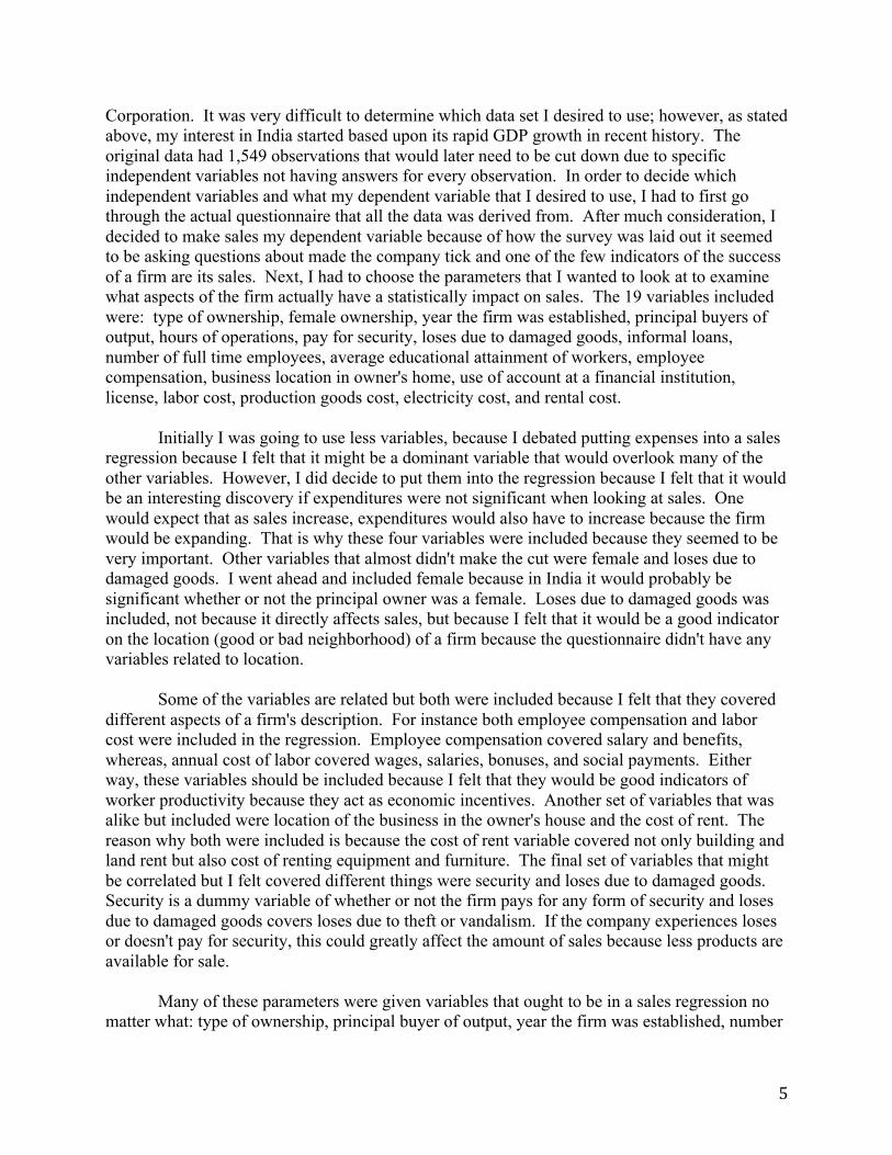
Corporation. It was very difficult to determine which data set I desired to use; however, as stated above, my interest in India started based upon its rapid GDP growth in recent history. The original data had 1,549 observations that would later need to be cut down due to specific independent variables not having answers for every observation. In order to decide which independent variables and what my dependent variable that I desired to use, I had to first go through the actual questionnaire that all the data was derived from. After much consideration, I decided to make sales my dependent variable because of how the survey was laid out it seemed to be asking questions about made the company tick and one of the few indicators of the success of a firm are its sales. Next, I had to choose the parameters that I wanted to look at to examine what aspects of the firm actually have a statistically impact on sales. The 19 variables included were: type of ownership, female ownership, year the firm was established, principal buyers of output, hours of operations, pay for security, loses due to damaged goods, informal loans, number of full time employees, average educational attainment of workers, employee compensation, business location in owner's home, use of account at a financial institution, license, labor cost, production goods cost, electricity cost, and rental cost. Initially I was going to use less variables, because I debated putting expenses into a sales regression because I felt that it might be a dominant variable that would overlook many of the other variables. However, I did decide to put them into the regression because I felt that it would be an interesting discovery if expenditures were not significant when looking at sales. One would expect that as sales increase, expenditures would also have to increase because the firm would be expanding. That is why these four variables were included because they seemed to be very important. Other variables that almost didn't make the cut were female and loses due to damaged goods. I went ahead and included female because in India it would probably be significant whether or not the principal owner was a female. Loses due to damaged goods was included, not because it directly affects sales, but because I felt that it would be a good indicator on the location (good or bad neighborhood) of a firm because the questionnaire didn't have any variables related to location. Some of the variables are related but both were included because I felt that they covered different aspects of a firm's description. For instance both employee compensation and labor cost were included in the regression. Employee compensation covered salary and benefits, whereas, annual cost of labor covered wages, salaries, bonuses, and social payments. Either way, these variables should be included because I felt that they would be good indicators of worker productivity because they act as economic incentives. Another set of variables that was alike but included were location of the business in the owner's house and the cost of rent. The reason why both were included is because the cost of rent variable covered not only building and land rent but also cost of renting equipment and furniture. The final set of variables that might be correlated but I felt covered different things were security and loses due to damaged goods. Security is a dummy variable of whether or not the firm pays for any form of security and loses due to damaged goods covers loses due to theft or vandalism. If the company experiences loses or doesn't pay for security, this could greatly affect the amount of sales because less products are available for sale. Many of these parameters were given variables that ought to be in a sales regression no matter what: type of ownership, principal buyer of output, year the firm was established, number

6

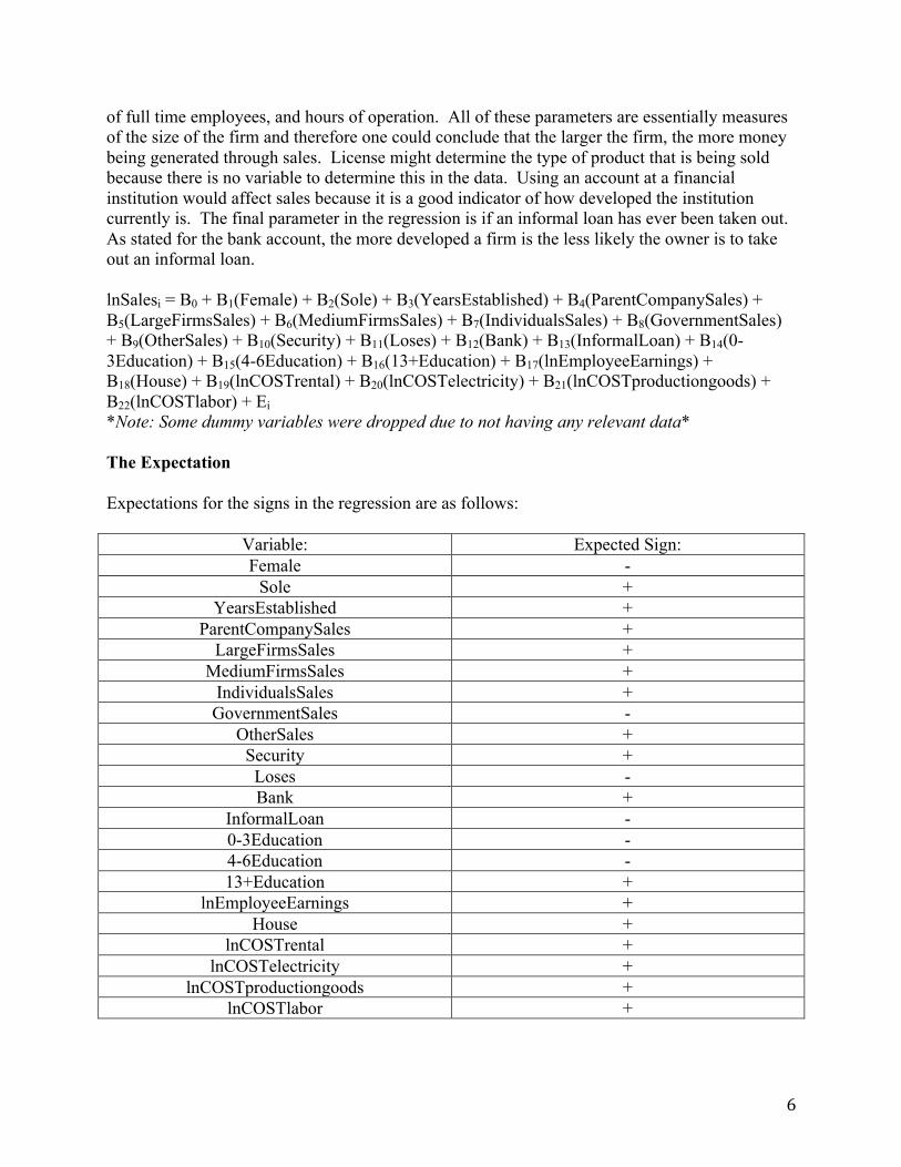
of full time employees, and hours of operation. All of these parameters are essentially measures of the size of the firm and therefore one could conclude that the larger the firm, the more money being generated through sales. License might determine the type of product that is being sold because there is no variable to determine this in the data. Using an account at a financial institution would affect sales because it is a good indicator of how developed the institution currently is. The final parameter in the regression is if an informal loan has ever been taken out. As stated for the bank account, the more developed a firm is the less likely the owner is to take out an informal loan. lnSalesi = B0 + B1(Female) + B2(Sole) + B3(YearsEstablished) + B4(ParentCompanySales) + B5(LargeFirmsSales) + B6(MediumFirmsSales) + B7(IndividualsSales) + B8(GovernmentSales) + B9(OtherSales) + B10(Security) + B11(Loses) + B12(Bank) + B13(InformalLoan) + B14(0-3Education) + B15(4-6Education) + B16(13+Education) + B17(lnEmployeeEarnings) + B18(House) + B19(lnCOSTrental) + B20(lnCOSTelectricity) + B21(lnCOSTproductiongoods) + B22(lnCOSTlabor) + Ei *Note: Some dummy variables were dropped due to not having any relevant data* The Expectation Expectations for the signs in the regression are as follows:

Variable: Expected Sign: Female -

Sole + YearsEstablished +

ParentCompanySales + LargeFirmsSales +

MediumFirmsSales + IndividualsSales + GovernmentSales -

OtherSales + Security + Loses - Bank +

InformalLoan - 0-3Education - 4-6Education - 13+Education +

lnEmployeeEarnings + House +

lnCOSTrental + lnCOSTelectricity +

lnCOSTproductiongoods + lnCOSTlabor +

7

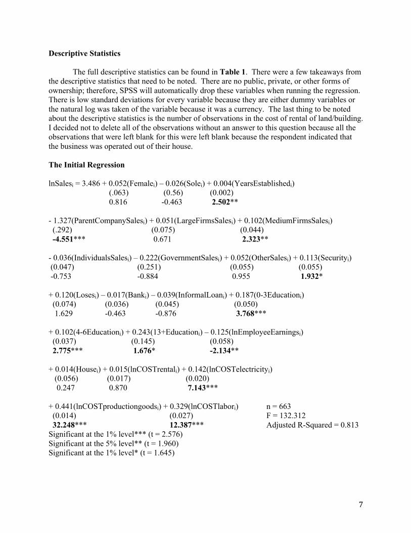
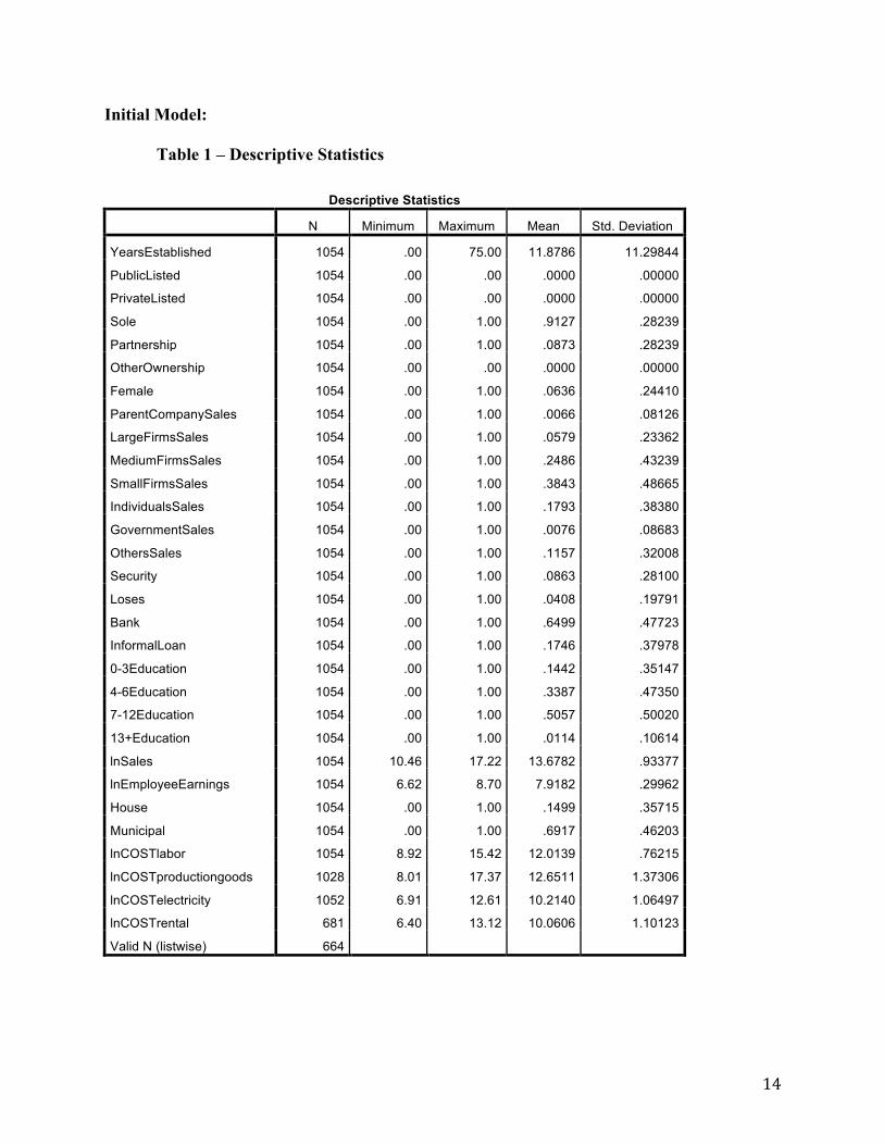
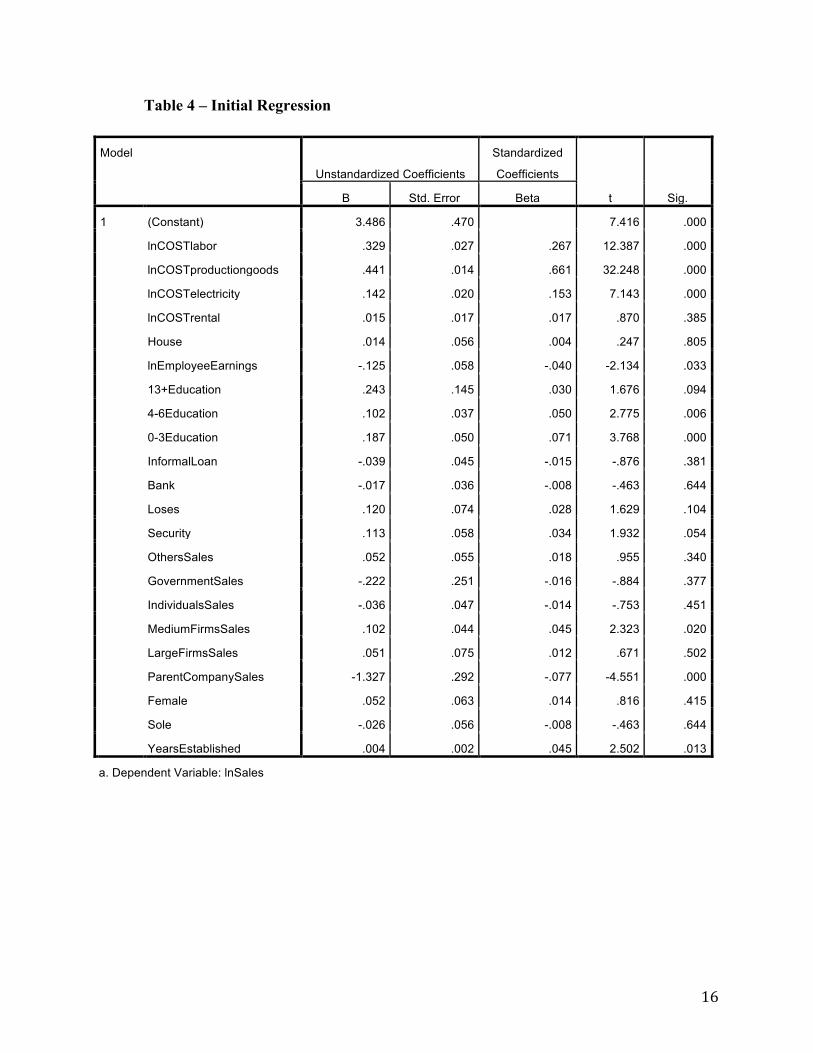
Descriptive Statistics The full descriptive statistics can be found in Table 1. There were a few takeaways from the descriptive statistics that need to be noted. There are no public, private, or other forms of ownership; therefore, SPSS will automatically drop these variables when running the regression. There is low standard deviations for every variable because they are either dummy variables or the natural log was taken of the variable because it was a currency. The last thing to be noted about the descriptive statistics is the number of observations in the cost of rental of land/building. I decided not to delete all of the observations without an answer to this question because all the observations that were left blank for this were left blank because the respondent indicated that the business was operated out of their house. The Initial Regression lnSalesi = 3.486 + 0.052(Femalei) – 0.026(Solei) + 0.004(YearsEstablishedi) (.063) (0.56) (0.002) 0.816 -0.463 2.502** - 1.327(ParentCompanySalesi) + 0.051(LargeFirmsSalesi) + 0.102(MediumFirmsSalesi) (.292) (0.075) (0.044) -4.551*** 0.671 2.323** - 0.036(IndividualsSalesi) – 0.222(GovernmentSalesi) + 0.052(OtherSalesi) + 0.113(Securityi) (0.047) (0.251) (0.055) (0.055) -0.753 -0.884 0.955 1.932* + 0.120(Losesi) – 0.017(Banki) – 0.039(InformalLoani) + 0.187(0-3Educationi) (0.074) (0.036) (0.045) (0.050) 1.629 -0.463 -0.876 3.768*** + 0.102(4-6Educationi) + 0.243(13+Educationi) – 0.125(lnEmployeeEarningsi) (0.037) (0.145) (0.058) 2.775*** 1.676* -2.134** + 0.014(Housei) + 0.015(lnCOSTrentali) + 0.142(lnCOSTelectricityi) (0.056) (0.017) (0.020) 0.247 0.870 7.143*** + 0.441(lnCOSTproductiongoodsi) + 0.329(lnCOSTlabori) n = 663 (0.014) (0.027) F = 132.312 32.248*** 12.387*** Adjusted R-Squared = 0.813 Significant at the 1% level*** (t = 2.576) Significant at the 5% level** (t = 1.960) Significant at the 1% level* (t = 1.645)

8

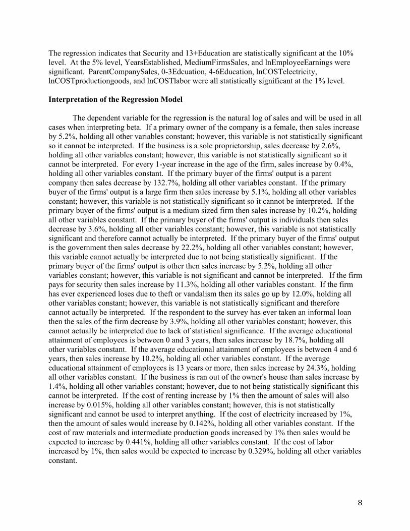
The regression indicates that Security and 13+Education are statistically significant at the 10% level. At the 5% level, YearsEstablished, MediumFirmsSales, and lnEmployeeEarnings were significant. ParentCompanySales, 0-3Edcuation, 4-6Education, lnCOSTelectricity, lnCOSTproductiongoods, and lnCOSTlabor were all statistically significant at the 1% level. Interpretation of the Regression Model The dependent variable for the regression is the natural log of sales and will be used in all cases when interpreting beta. If a primary owner of the company is a female, then sales increase by 5.2%, holding all other variables constant; however, this variable is not statistically significant so it cannot be interpreted. If the business is a sole proprietorship, sales decrease by 2.6%, holding all other variables constant; however, this variable is not statistically significant so it cannot be interpreted. For every 1-year increase in the age of the firm, sales increase by 0.4%, holding all other variables constant. If the primary buyer of the firms' output is a parent company then sales decrease by 132.7%, holding all other variables constant. If the primary buyer of the firms' output is a large firm then sales increase by 5.1%, holding all other variables constant; however, this variable is not statistically significant so it cannot be interpreted. If the primary buyer of the firms' output is a medium sized firm then sales increase by 10.2%, holding all other variables constant. If the primary buyer of the firms' output is individuals then sales decrease by 3.6%, holding all other variables constant; however, this variable is not statistically significant and therefore cannot actually be interpreted. If the primary buyer of the firms' output is the government then sales decrease by 22.2%, holding all other variables constant; however, this variable cannot actually be interpreted due to not being statistically significant. If the primary buyer of the firms' output is other then sales increase by 5.2%, holding all other variables constant; however, this variable is not significant and cannot be interpreted. If the firm pays for security then sales increase by 11.3%, holding all other variables constant. If the firm has ever experienced loses due to theft or vandalism then its sales go up by 12.0%, holding all other variables constant; however, this variable is not statistically significant and therefore cannot actually be interpreted. If the respondent to the survey has ever taken an informal loan then the sales of the firm decrease by 3.9%, holding all other variables constant; however, this cannot actually be interpreted due to lack of statistical significance. If the average educational attainment of employees is between 0 and 3 years, then sales increase by 18.7%, holding all other variables constant. If the average educational attainment of employees is between 4 and 6 years, then sales increase by 10.2%, holding all other variables constant. If the average educational attainment of employees is 13 years or more, then sales increase by 24.3%, holding all other variables constant. If the business is ran out of the owner's house than sales increase by 1.4%, holding all other variables constant; however, due to not being statistically significant this cannot be interpreted. If the cost of renting increase by 1% then the amount of sales will also increase by 0.015%, holding all other variables constant; however, this is not statistically significant and cannot be used to interpret anything. If the cost of electricity increased by 1%, then the amount of sales would increase by 0.142%, holding all other variables constant. If the cost of raw materials and intermediate production goods increased by 1% then sales would be expected to increase by 0.441%, holding all other variables constant. If the cost of labor increased by 1%, then sales would be expected to increase by 0.329%, holding all other variables constant.

9

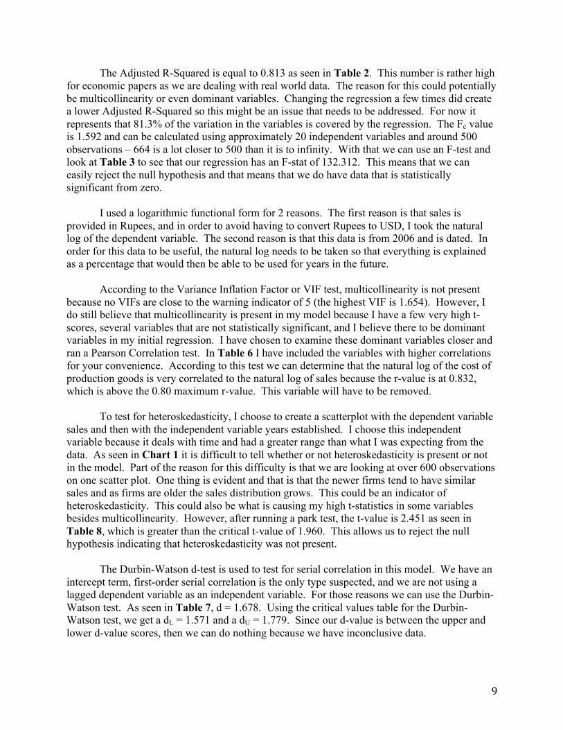
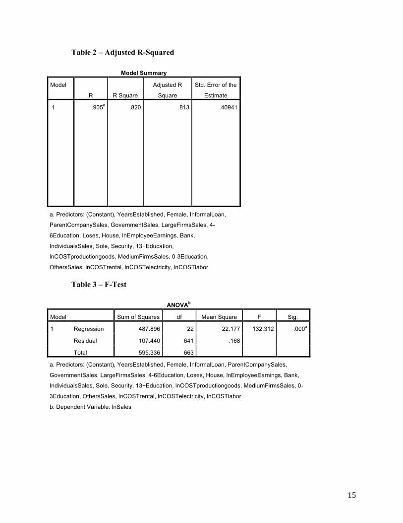
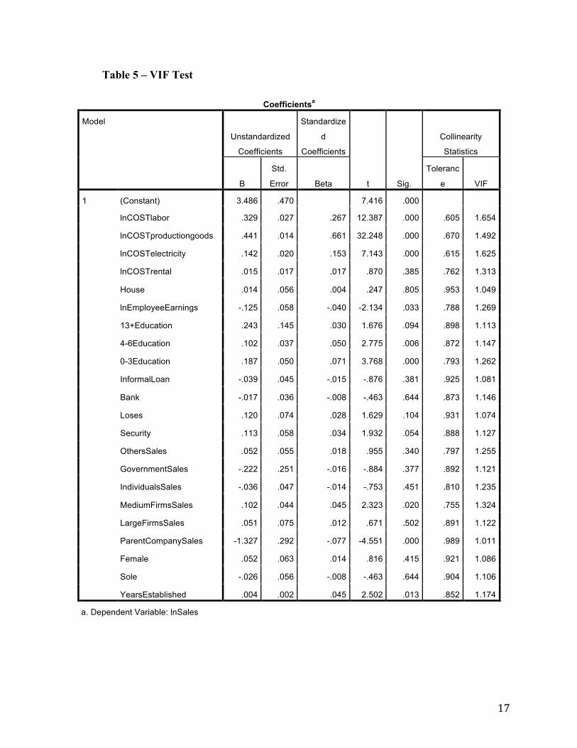
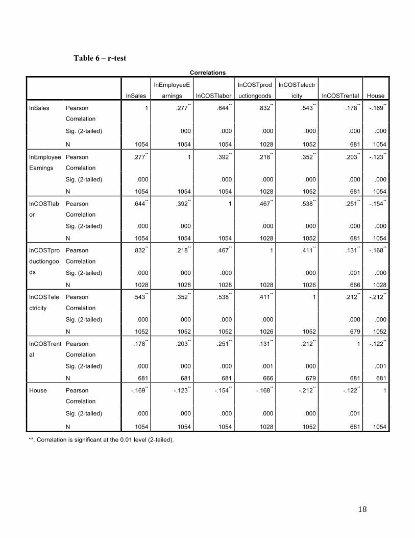
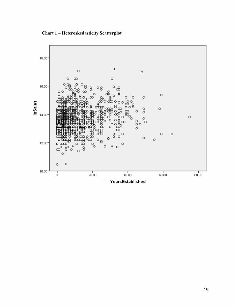
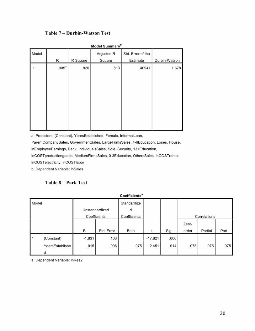
The Adjusted R-Squared is equal to 0.813 as seen in Table 2. This number is rather high for economic papers as we are dealing with real world data. The reason for this could potentially be multicollinearity or even dominant variables. Changing the regression a few times did create a lower Adjusted R-Squared so this might be an issue that needs to be addressed. For now it represents that 81.3% of the variation in the variables is covered by the regression. The Fc value is 1.592 and can be calculated using approximately 20 independent variables and around 500 observations – 664 is a lot closer to 500 than it is to infinity. With that we can use an F-test and look at Table 3 to see that our regression has an F-stat of 132.312. This means that we can easily reject the null hypothesis and that means that we do have data that is statistically significant from zero. I used a logarithmic functional form for 2 reasons. The first reason is that sales is provided in Rupees, and in order to avoid having to convert Rupees to USD, I took the natural log of the dependent variable. The second reason is that this data is from 2006 and is dated. In order for this data to be useful, the natural log needs to be taken so that everything is explained as a percentage that would then be able to be used for years in the future. According to the Variance Inflation Factor or VIF test, multicollinearity is not present because no VIFs are close to the warning indicator of 5 (the highest VIF is 1.654). However, I do still believe that multicollinearity is present in my model because I have a few very high t-scores, several variables that are not statistically significant, and I believe there to be dominant variables in my initial regression. I have chosen to examine these dominant variables closer and ran a Pearson Correlation test. In Table 6 I have included the variables with higher correlations for your convenience. According to this test we can determine that the natural log of the cost of production goods is very correlated to the natural log of sales because the r-value is at 0.832, which is above the 0.80 maximum r-value. This variable will have to be removed. To test for heteroskedasticity, I choose to create a scatterplot with the dependent variable sales and then with the independent variable years established. I choose this independent variable because it deals with time and had a greater range than what I was expecting from the data. As seen in Chart 1 it is difficult to tell whether or not heteroskedasticity is present or not in the model. Part of the reason for this difficulty is that we are looking at over 600 observations on one scatter plot. One thing is evident and that is that the newer firms tend to have similar sales and as firms are older the sales distribution grows. This could be an indicator of heteroskedasticity. This could also be what is causing my high t-statistics in some variables besides multicollinearity. However, after running a park test, the t-value is 2.451 as seen in Table 8, which is greater than the critical t-value of 1.960. This allows us to reject the null hypothesis indicating that heteroskedasticity was not present. The Durbin-Watson d-test is used to test for serial correlation in this model. We have an intercept term, first-order serial correlation is the only type suspected, and we are not using a lagged dependent variable as an independent variable. For those reasons we can use the Durbin-Watson test. As seen in Table 7, d = 1.678. Using the critical values table for the Durbin-Watson test, we get a dL = 1.571 and a dU = 1.779. Since our d-value is between the upper and lower d-value scores, then we can do nothing because we have inconclusive data.

10

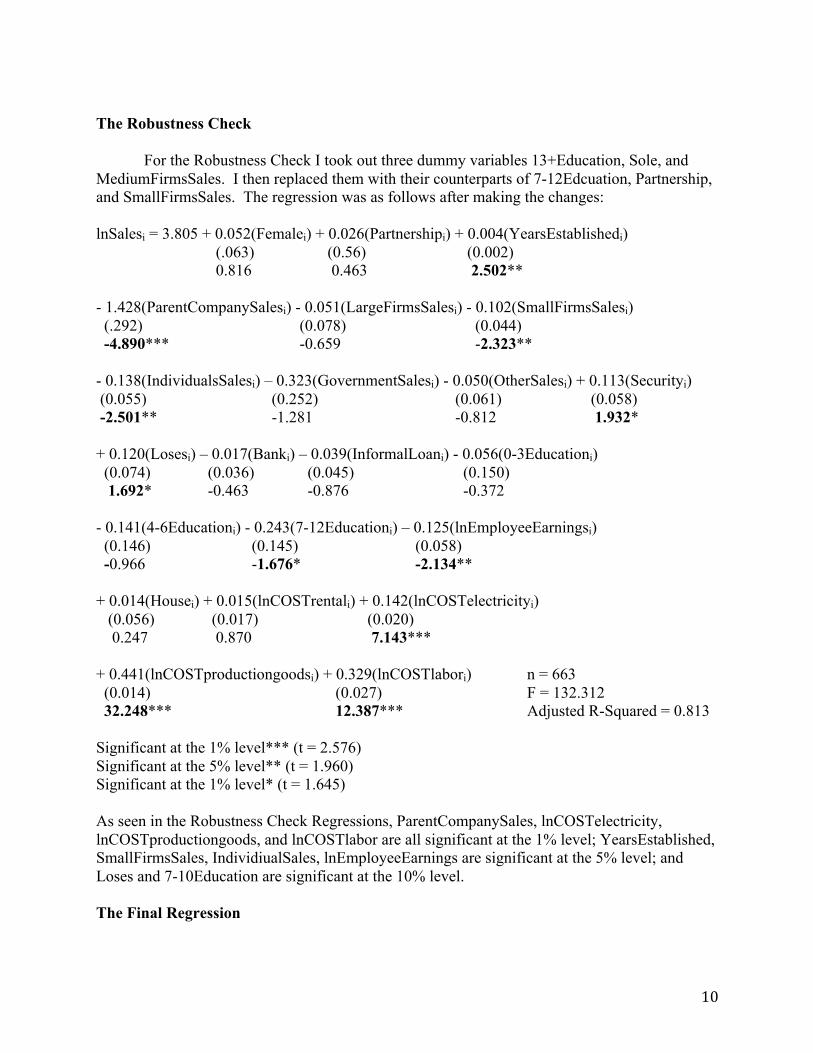
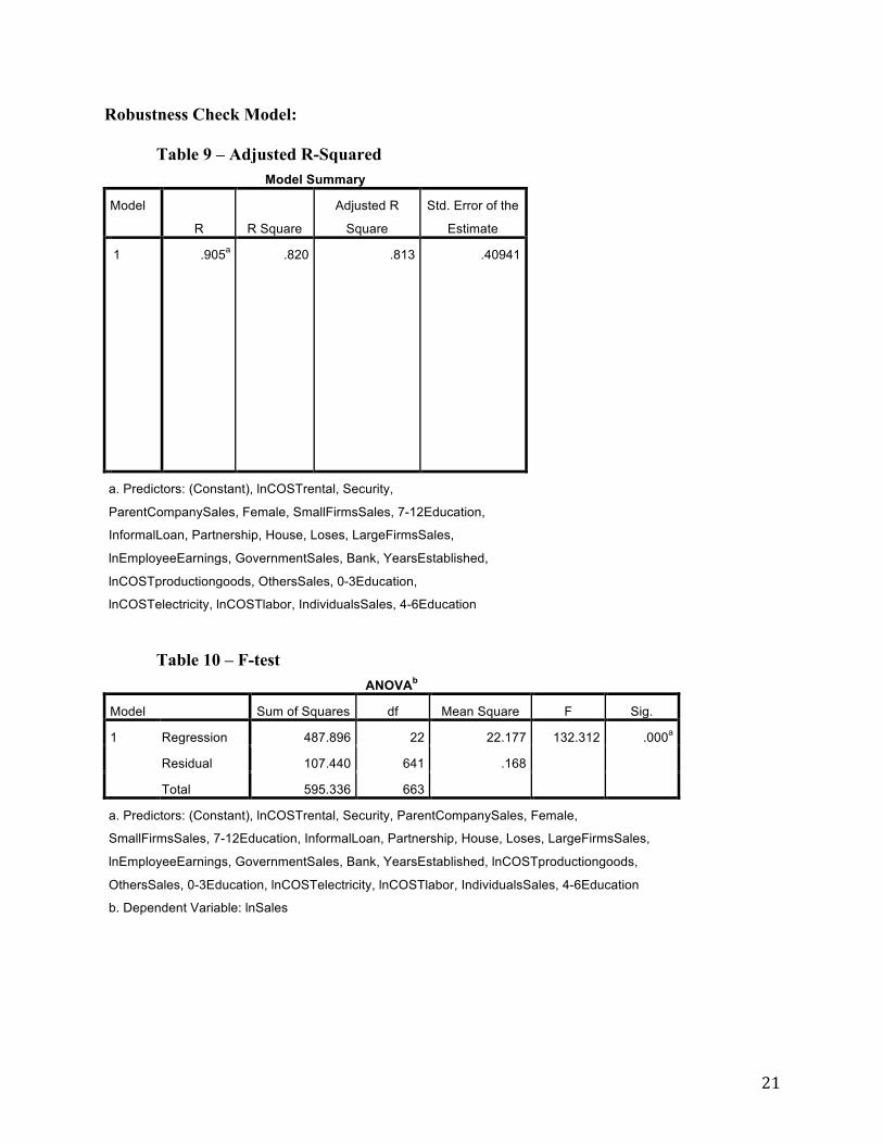
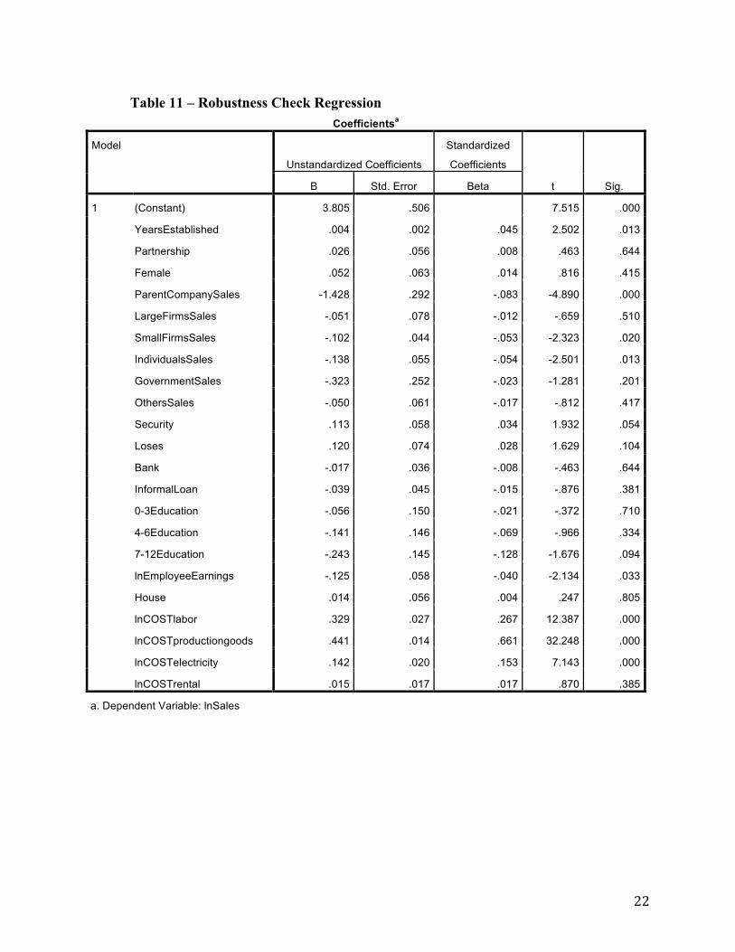
The Robustness Check For the Robustness Check I took out three dummy variables 13+Education, Sole, and MediumFirmsSales. I then replaced them with their counterparts of 7-12Edcuation, Partnership, and SmallFirmsSales. The regression was as follows after making the changes: lnSalesi = 3.805 + 0.052(Femalei) + 0.026(Partnershipi) + 0.004(YearsEstablishedi) (.063) (0.56) (0.002) 0.816 0.463 2.502** - 1.428(ParentCompanySalesi) - 0.051(LargeFirmsSalesi) - 0.102(SmallFirmsSalesi) (.292) (0.078) (0.044) -4.890*** -0.659 -2.323** - 0.138(IndividualsSalesi) – 0.323(GovernmentSalesi) - 0.050(OtherSalesi) + 0.113(Securityi) (0.055) (0.252) (0.061) (0.058) -2.501** -1.281 -0.812 1.932* + 0.120(Losesi) – 0.017(Banki) – 0.039(InformalLoani) - 0.056(0-3Educationi) (0.074) (0.036) (0.045) (0.150) 1.692* -0.463 -0.876 -0.372 - 0.141(4-6Educationi) - 0.243(7-12Educationi) – 0.125(lnEmployeeEarningsi) (0.146) (0.145) (0.058) -0.966 -1.676* -2.134** + 0.014(Housei) + 0.015(lnCOSTrentali) + 0.142(lnCOSTelectricityi) (0.056) (0.017) (0.020) 0.247 0.870 7.143*** + 0.441(lnCOSTproductiongoodsi) + 0.329(lnCOSTlabori) n = 663 (0.014) (0.027) F = 132.312 32.248*** 12.387*** Adjusted R-Squared = 0.813 Significant at the 1% level*** (t = 2.576) Significant at the 5% level** (t = 1.960) Significant at the 1% level* (t = 1.645) As seen in the Robustness Check Regressions, ParentCompanySales, lnCOSTelectricity, lnCOSTproductiongoods, and lnCOSTlabor are all significant at the 1% level; YearsEstablished, SmallFirmsSales, IndividiualSales, lnEmployeeEarnings are significant at the 5% level; and Loses and 7-10Education are significant at the 10% level. The Final Regression

11

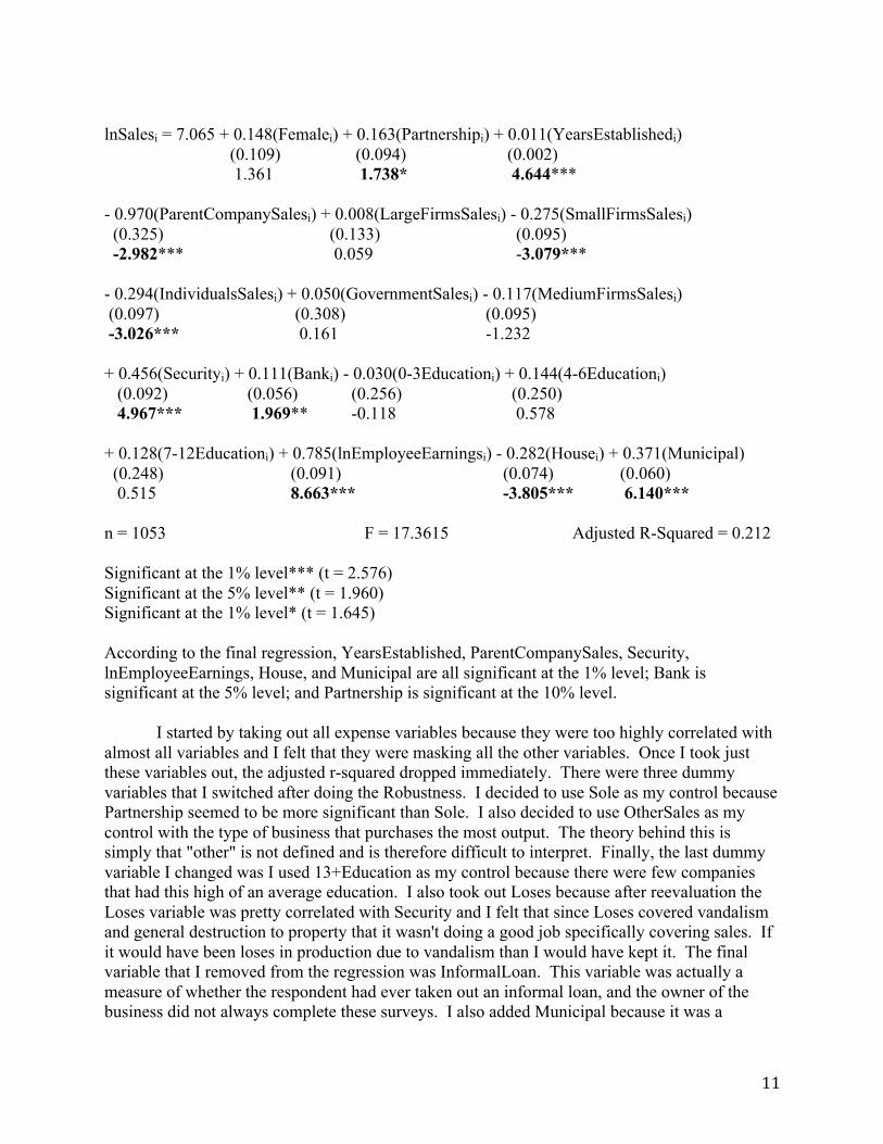
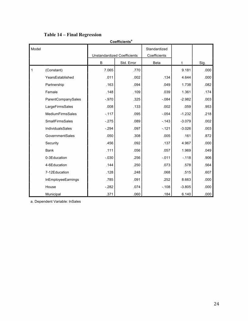
lnSalesi = 7.065 + 0.148(Femalei) + 0.163(Partnershipi) + 0.011(YearsEstablishedi) (0.109) (0.094) (0.002) 1.361 1.738* 4.644*** - 0.970(ParentCompanySalesi) + 0.008(LargeFirmsSalesi) - 0.275(SmallFirmsSalesi) (0.325) (0.133) (0.095) -2.982*** 0.059 -3.079*** - 0.294(IndividualsSalesi) + 0.050(GovernmentSalesi) - 0.117(MediumFirmsSalesi) (0.097) (0.308) (0.095) -3.026*** 0.161 -1.232 + 0.456(Securityi) + 0.111(Banki) - 0.030(0-3Educationi) + 0.144(4-6Educationi) (0.092) (0.056) (0.256) (0.250) 4.967*** 1.969** -0.118 0.578 + 0.128(7-12Educationi) + 0.785(lnEmployeeEarningsi) - 0.282(Housei) + 0.371(Municipal) (0.248) (0.091) (0.074) (0.060) 0.515 8.663*** -3.805*** 6.140*** n = 1053 F = 17.3615 Adjusted R-Squared = 0.212 Significant at the 1% level*** (t = 2.576) Significant at the 5% level** (t = 1.960) Significant at the 1% level* (t = 1.645) According to the final regression, YearsEstablished, ParentCompanySales, Security, lnEmployeeEarnings, House, and Municipal are all significant at the 1% level; Bank is significant at the 5% level; and Partnership is significant at the 10% level. I started by taking out all expense variables because they were too highly correlated with almost all variables and I felt that they were masking all the other variables. Once I took just these variables out, the adjusted r-squared dropped immediately. There were three dummy variables that I switched after doing the Robustness. I decided to use Sole as my control because Partnership seemed to be more significant than Sole. I also decided to use OtherSales as my control with the type of business that purchases the most output. The theory behind this is simply that "other" is not defined and is therefore difficult to interpret. Finally, the last dummy variable I changed was I used 13+Education as my control because there were few companies that had this high of an average education. I also took out Loses because after reevaluation the Loses variable was pretty correlated with Security and I felt that since Loses covered vandalism and general destruction to property that it wasn't doing a good job specifically covering sales. If it would have been loses in production due to vandalism than I would have kept it. The final variable that I removed from the regression was InformalLoan. This variable was actually a measure of whether the respondent had ever taken out an informal loan, and the owner of the business did not always complete these surveys. I also added Municipal because it was a

12

variable that indicated whether or not the firm was a legal establishment. I felt that it would be important in determining sales because it limits whom the firm can sale to.

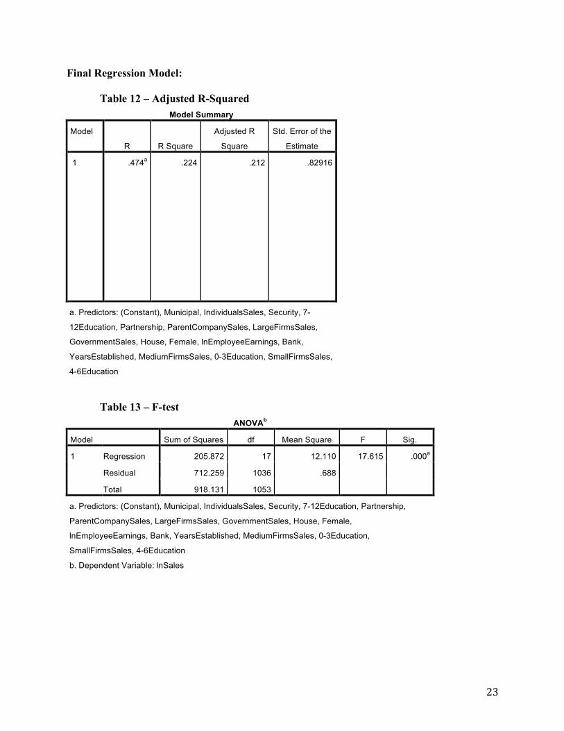
Overall, Adjusted R-squared dropped from 0.813 (Table 2) to 0.212 (Table 12). This indicates that I was able to remove the multicollinearity and the dominant variable that was overpowering the data. The F-score decreased from 132.312 (Table 3) to 17.615 (Table 13) and the intercept term increased from 3.486 (Table 4) to 7.065 (Table 14). Normally you wouldn't want to see this change, but since I was eliminating multicollinearity and dominant variables I am fine with this change. After this regression I am much more satisfied than with my initial regression. I have reasonable t-scores, an all right adjusted r-squared and I agree with all of the current signs. Conclusions Sales is the driving factor that makes a business run. Without sales, firms cannot pay their expenses nor can they afford to continue operating. Overall several conclusions can be drawn from this data and can be applied in policy form. Education not being a factor in sales is surprising; however, employee compensation is significant at the 1% level so this is not as surprising. You would expect that your worker productivity affects how much you can produce and therefore how much you can sell. Other interesting findings include that female is almost significant at the 10% level. The reason why this is so interesting is because out of 1053 observations only 82 had female owners; yet, it was still almost statistically significant. What makes the female variable even more interesting to me is that it is positive – the opposite of what I expected. The biggest ways to increase sales from a microeconomic viewpoint would be to ensure that the government registers the firm, increase your employee compensation (therefore increasing economic incentives to work harder), and ensure that you have some form of security to protect all assets. There are numerous ways that future research could be conducted on this matter. You could of course always change the country – Enterprise Surveys has this same survey for numerous other countries. Even more interesting however would be to look at our previous dominant variable of the natural log of the cost of production goods and make it the dependent variable. Then you would be able to how a firm can decrease expenses and through decreasing expenses you would then be able to analyze the impact of profit because it is revenue minuses expenses. Of course, more detail can be put into the current regression as well. It must be understood that this is not a perfect regression; however, making a few changes would not adversely affect anything.

13

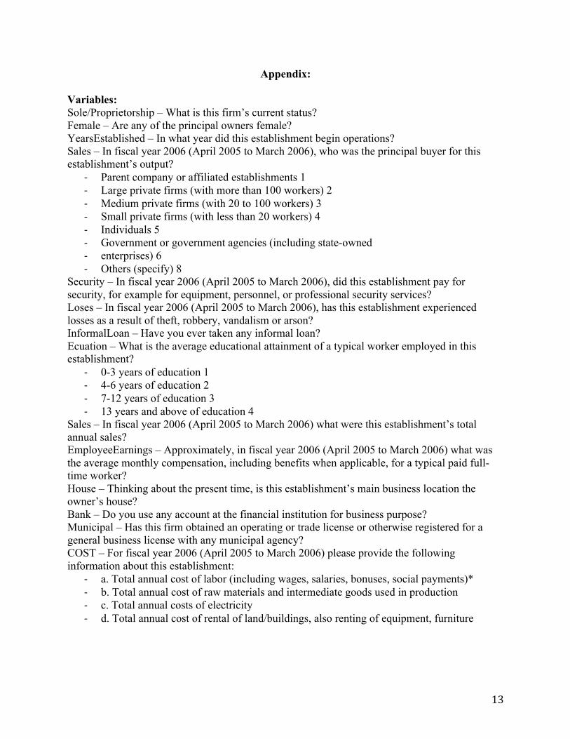
Appendix: Variables: Sole/Proprietorship – What is this firm’s current status? Female – Are any of the principal owners female? YearsEstablished – In what year did this establishment begin operations? Sales – In fiscal year 2006 (April 2005 to March 2006), who was the principal buyer for this establishment’s output?

- Parent company or affiliated establishments 1 - Large private firms (with more than 100 workers) 2 - Medium private firms (with 20 to 100 workers) 3 - Small private firms (with less than 20 workers) 4 - Individuals 5 - Government or government agencies (including state-owned - enterprises) 6 - Others (specify) 8

Security – In fiscal year 2006 (April 2005 to March 2006), did this establishment pay for security, for example for equipment, personnel, or professional security services? Loses – In fiscal year 2006 (April 2005 to March 2006), has this establishment experienced losses as a result of theft, robbery, vandalism or arson? InformalLoan – Have you ever taken any informal loan? Ecuation – What is the average educational attainment of a typical worker employed in this establishment?

- 0-3 years of education 1 - 4-6 years of education 2 - 7-12 years of education 3 - 13 years and above of education 4

Sales – In fiscal year 2006 (April 2005 to March 2006) what were this establishment’s total annual sales? EmployeeEarnings – Approximately, in fiscal year 2006 (April 2005 to March 2006) what was the average monthly compensation, including benefits when applicable, for a typical paid full-time worker? House – Thinking about the present time, is this establishment’s main business location the owner’s house? Bank – Do you use any account at the financial institution for business purpose? Municipal – Has this firm obtained an operating or trade license or otherwise registered for a general business license with any municipal agency? COST – For fiscal year 2006 (April 2005 to March 2006) please provide the following information about this establishment:

- a. Total annual cost of labor (including wages, salaries, bonuses, social payments)* - b. Total annual cost of raw materials and intermediate goods used in production - c. Total annual costs of electricity - d. Total annual cost of rental of land/buildings, also renting of equipment, furniture

14

Initial Model: Table 1 – Descriptive Statistics

Descriptive Statistics

N Minimum Maximum Mean Std. Deviation

YearsEstablished 1054 .00 75.00 11.8786 11.29844

PublicListed 1054 .00 .00 .0000 .00000

PrivateListed 1054 .00 .00 .0000 .00000

Sole 1054 .00 1.00 .9127 .28239

Partnership 1054 .00 1.00 .0873 .28239

OtherOwnership 1054 .00 .00 .0000 .00000

Female 1054 .00 1.00 .0636 .24410

ParentCompanySales 1054 .00 1.00 .0066 .08126

LargeFirmsSales 1054 .00 1.00 .0579 .23362

MediumFirmsSales 1054 .00 1.00 .2486 .43239

SmallFirmsSales 1054 .00 1.00 .3843 .48665

IndividualsSales 1054 .00 1.00 .1793 .38380

GovernmentSales 1054 .00 1.00 .0076 .08683

OthersSales 1054 .00 1.00 .1157 .32008

Security 1054 .00 1.00 .0863 .28100

Loses 1054 .00 1.00 .0408 .19791

Bank 1054 .00 1.00 .6499 .47723

InformalLoan 1054 .00 1.00 .1746 .37978

0-3Education 1054 .00 1.00 .1442 .35147

4-6Education 1054 .00 1.00 .3387 .47350

7-12Education 1054 .00 1.00 .5057 .50020

13+Education 1054 .00 1.00 .0114 .10614

lnSales 1054 10.46 17.22 13.6782 .93377

lnEmployeeEarnings 1054 6.62 8.70 7.9182 .29962

House 1054 .00 1.00 .1499 .35715

Municipal 1054 .00 1.00 .6917 .46203

lnCOSTlabor 1054 8.92 15.42 12.0139 .76215

lnCOSTproductiongoods 1028 8.01 17.37 12.6511 1.37306

lnCOSTelectricity 1052 6.91 12.61 10.2140 1.06497

lnCOSTrental 681 6.40 13.12 10.0606 1.10123

Valid N (listwise) 664

15

Table 2 – Adjusted R-Squared

Model Summary

Model

R R Square

Adjusted R

Square

Std. Error of the

Estimate

d

i

m

e

n

s

i

o

n

0

1 .905a .820 .813 .40941

a. Predictors: (Constant), YearsEstablished, Female, InformalLoan,

ParentCompanySales, GovernmentSales, LargeFirmsSales, 4-

6Education, Loses, House, lnEmployeeEarnings, Bank,

IndividualsSales, Sole, Security, 13+Education,

lnCOSTproductiongoods, MediumFirmsSales, 0-3Education,

OthersSales, lnCOSTrental, lnCOSTelectricity, lnCOSTlabor Table 3 – F-Test

ANOVAb

Model Sum of Squares df Mean Square F Sig.

1 Regression 487.896 22 22.177 132.312 .000a

Residual 107.440 641 .168 Total 595.336 663

a. Predictors: (Constant), YearsEstablished, Female, InformalLoan, ParentCompanySales,

GovernmentSales, LargeFirmsSales, 4-6Education, Loses, House, lnEmployeeEarnings, Bank,

IndividualsSales, Sole, Security, 13+Education, lnCOSTproductiongoods, MediumFirmsSales, 0-

3Education, OthersSales, lnCOSTrental, lnCOSTelectricity, lnCOSTlabor

b. Dependent Variable: lnSales

16

Table 4 – Initial Regression

Model

Unstandardized Coefficients

Standardized

Coefficients

t Sig. B Std. Error Beta

1 (Constant) 3.486 .470 7.416 .000

lnCOSTlabor .329 .027 .267 12.387 .000

lnCOSTproductiongoods .441 .014 .661 32.248 .000

lnCOSTelectricity .142 .020 .153 7.143 .000

lnCOSTrental .015 .017 .017 .870 .385

House .014 .056 .004 .247 .805

lnEmployeeEarnings -.125 .058 -.040 -2.134 .033

13+Education .243 .145 .030 1.676 .094

4-6Education .102 .037 .050 2.775 .006

0-3Education .187 .050 .071 3.768 .000

InformalLoan -.039 .045 -.015 -.876 .381

Bank -.017 .036 -.008 -.463 .644

Loses .120 .074 .028 1.629 .104

Security .113 .058 .034 1.932 .054

OthersSales .052 .055 .018 .955 .340

GovernmentSales -.222 .251 -.016 -.884 .377

IndividualsSales -.036 .047 -.014 -.753 .451

MediumFirmsSales .102 .044 .045 2.323 .020

LargeFirmsSales .051 .075 .012 .671 .502

ParentCompanySales -1.327 .292 -.077 -4.551 .000

Female .052 .063 .014 .816 .415

Sole -.026 .056 -.008 -.463 .644

YearsEstablished .004 .002 .045 2.502 .013

a. Dependent Variable: lnSales

17

Table 5 – VIF Test

Coefficientsa

Model

Unstandardized

Coefficients

Standardize

d

Coefficients

t Sig.

Collinearity

Statistics

B

Std.

Error Beta

Toleranc

e VIF

1 (Constant) 3.486 .470 7.416 .000 lnCOSTlabor .329 .027 .267 12.387 .000 .605 1.654

lnCOSTproductiongoods .441 .014 .661 32.248 .000 .670 1.492

lnCOSTelectricity .142 .020 .153 7.143 .000 .615 1.625

lnCOSTrental .015 .017 .017 .870 .385 .762 1.313

House .014 .056 .004 .247 .805 .953 1.049

lnEmployeeEarnings -.125 .058 -.040 -2.134 .033 .788 1.269

13+Education .243 .145 .030 1.676 .094 .898 1.113

4-6Education .102 .037 .050 2.775 .006 .872 1.147

0-3Education .187 .050 .071 3.768 .000 .793 1.262

InformalLoan -.039 .045 -.015 -.876 .381 .925 1.081

Bank -.017 .036 -.008 -.463 .644 .873 1.146

Loses .120 .074 .028 1.629 .104 .931 1.074

Security .113 .058 .034 1.932 .054 .888 1.127

OthersSales .052 .055 .018 .955 .340 .797 1.255

GovernmentSales -.222 .251 -.016 -.884 .377 .892 1.121

IndividualsSales -.036 .047 -.014 -.753 .451 .810 1.235

MediumFirmsSales .102 .044 .045 2.323 .020 .755 1.324

LargeFirmsSales .051 .075 .012 .671 .502 .891 1.122

ParentCompanySales -1.327 .292 -.077 -4.551 .000 .989 1.011

Female .052 .063 .014 .816 .415 .921 1.086

Sole -.026 .056 -.008 -.463 .644 .904 1.106

YearsEstablished .004 .002 .045 2.502 .013 .852 1.174


18

Table 6 – r-test

Correlations

lnSales

lnEmployeeE

arnings lnCOSTlabor

lnCOSTprod

uctiongoods

lnCOSTelectr

icity lnCOSTrental House

lnSales Pearson

Correlation

1 .277** .644** .832** .543** .178** -.169**

Sig. (2-tailed) .000 .000 .000 .000 .000 .000

N 1054 1054 1054 1028 1052 681 1054

lnEmployee

Earnings

Pearson

Correlation

.277** 1 .392** .218** .352** .203** -.123**

Sig. (2-tailed) .000 .000 .000 .000 .000 .000

N 1054 1054 1054 1028 1052 681 1054

lnCOSTlab

or

Pearson

Correlation

.644** .392** 1 .467** .538** .251** -.154**

Sig. (2-tailed) .000 .000 .000 .000 .000 .000

N 1054 1054 1054 1028 1052 681 1054

lnCOSTpro

ductiongoo

ds

Pearson

Correlation

.832** .218** .467** 1 .411** .131** -.168**

Sig. (2-tailed) .000 .000 .000 .000 .001 .000

N 1028 1028 1028 1028 1026 666 1028

lnCOSTele

ctricity

Pearson

Correlation

.543** .352** .538** .411** 1 .212** -.212**

Sig. (2-tailed) .000 .000 .000 .000 .000 .000

N 1052 1052 1052 1026 1052 679 1052

lnCOSTrent

al

Pearson

Correlation

.178** .203** .251** .131** .212** 1 -.122**

Sig. (2-tailed) .000 .000 .000 .001 .000 .001

N 681 681 681 666 679 681 681

House Pearson

Correlation

-.169** -.123** -.154** -.168** -.212** -.122** 1

Sig. (2-tailed) .000 .000 .000 .000 .000 .001

N 1054 1054 1054 1028 1052 681 1054

**. Correlation is significant at the 0.01 level (2-tailed).

19

Chart 1 – Heteroskedasticity Scatterplot

20

Table 7 – Durbin-Watson Test

Model Summaryb

Model

R R Square

Adjusted R

Square

Std. Error of the

Estimate Durbin-Watson

d

i

m

e

n

s

i

o

n

0

1 .905a .820 .813 .40941 1.678

a. Predictors: (Constant), YearsEstablished, Female, InformalLoan,

ParentCompanySales, GovernmentSales, LargeFirmsSales, 4-6Education, Loses, House,

lnEmployeeEarnings, Bank, IndividualsSales, Sole, Security, 13+Education,

lnCOSTproductiongoods, MediumFirmsSales, 0-3Education, OthersSales, lnCOSTrental,

lnCOSTelectricity, lnCOSTlabor


Table 8 – Park Test

Coefficientsa

Model

Unstandardized

Coefficients

Standardize

d

Coefficients

t Sig.

Correlations

B Std. Error Beta

Zero-

order Partial Part

1 (Constant) -1.831 .103 -17.821 .000 YearsEstablishe

d

.015 .006 .075 2.451 .014 .075 .075 .075

a. Dependent Variable: lnRes2

21

Robustness Check Model:

Table 9 – Adjusted R-Squared Model Summary

Model

R R Square

Adjusted R

Square

Std. Error of the

Estimate

d

i

m

e

n

s

i

o

n

0

1 .905a .820 .813 .40941

a. Predictors: (Constant), lnCOSTrental, Security,

ParentCompanySales, Female, SmallFirmsSales, 7-12Education,

InformalLoan, Partnership, House, Loses, LargeFirmsSales,

lnEmployeeEarnings, GovernmentSales, Bank, YearsEstablished,

lnCOSTproductiongoods, OthersSales, 0-3Education,

lnCOSTelectricity, lnCOSTlabor, IndividualsSales, 4-6Education

Table 10 – F-test ANOVAb


1 Regression 487.896 22 22.177 132.312 .000a

Residual 107.440 641 .168

Total 595.336 663

a. Predictors: (Constant), lnCOSTrental, Security, ParentCompanySales, Female,

SmallFirmsSales, 7-12Education, InformalLoan, Partnership, House, Loses, LargeFirmsSales,

lnEmployeeEarnings, GovernmentSales, Bank, YearsEstablished, lnCOSTproductiongoods,

OthersSales, 0-3Education, lnCOSTelectricity, lnCOSTlabor, IndividualsSales, 4-6Education


22

Table 11 – Robustness Check Regression Coefficientsa

Model


Standardized

Coefficients


1 (Constant) 3.805 .506 7.515 .000


Partnership .026 .056 .008 .463 .644

Female .052 .063 .014 .816 .415

ParentCompanySales -1.428 .292 -.083 -4.890 .000

LargeFirmsSales -.051 .078 -.012 -.659 .510

SmallFirmsSales -.102 .044 -.053 -2.323 .020

IndividualsSales -.138 .055 -.054 -2.501 .013

GovernmentSales -.323 .252 -.023 -1.281 .201

OthersSales -.050 .061 -.017 -.812 .417

Security .113 .058 .034 1.932 .054

Loses .120 .074 .028 1.629 .104

Bank -.017 .036 -.008 -.463 .644

InformalLoan -.039 .045 -.015 -.876 .381

0-3Education -.056 .150 -.021 -.372 .710

4-6Education -.141 .146 -.069 -.966 .334

7-12Education -.243 .145 -.128 -1.676 .094

lnEmployeeEarnings -.125 .058 -.040 -2.134 .033

House .014 .056 .004 .247 .805

lnCOSTlabor .329 .027 .267 12.387 .000

lnCOSTproductiongoods .441 .014 .661 32.248 .000

lnCOSTelectricity .142 .020 .153 7.143 .000

lnCOSTrental .015 .017 .017 .870 .385


23

Final Regression Model:

Table 12 – Adjusted R-Squared Model Summary

Model

R R Square

Adjusted R

Square

Std. Error of the

Estimate

d

i

m

e

n

s

i

o

n

0

1 .474a .224 .212 .82916

a. Predictors: (Constant), Municipal, IndividualsSales, Security, 7-

12Education, Partnership, ParentCompanySales, LargeFirmsSales,

GovernmentSales, House, Female, lnEmployeeEarnings, Bank,

YearsEstablished, MediumFirmsSales, 0-3Education, SmallFirmsSales,

4-6Education

Table 13 – F-test ANOVAb


1 Regression 205.872 17 12.110 17.615 .000a

Residual 712.259 1036 .688 Total 918.131 1053

a. Predictors: (Constant), Municipal, IndividualsSales, Security, 7-12Education, Partnership,

ParentCompanySales, LargeFirmsSales, GovernmentSales, House, Female,

lnEmployeeEarnings, Bank, YearsEstablished, MediumFirmsSales, 0-3Education,

SmallFirmsSales, 4-6Education


24

Table 14 – Final Regression Coefficientsa

Model


Standardized

Coefficients


1 (Constant) 7.065 .770 9.181 .000


Partnership .163 .094 .049 1.738 .082

Female .148 .109 .039 1.361 .174

ParentCompanySales -.970 .325 -.084 -2.982 .003

LargeFirmsSales .008 .133 .002 .059 .953

MediumFirmsSales -.117 .095 -.054 -1.232 .218

SmallFirmsSales -.275 .089 -.143 -3.079 .002

IndividualsSales -.294 .097 -.121 -3.026 .003

GovernmentSales .050 .308 .005 .161 .872

Security .456 .092 .137 4.967 .000

Bank .111 .056 .057 1.969 .049

0-3Education -.030 .256 -.011 -.118 .906

4-6Education .144 .250 .073 .578 .564

7-12Education .128 .248 .068 .515 .607

lnEmployeeEarnings .785 .091 .252 8.663 .000

House -.282 .074 -.108 -3.805 .000

Municipal .371 .060 .184 6.140 .000


25

Works Cited

Bosworth, B., Collins, S., & Virmani, A. (2007). Sources of Growth in the Indian Economy. India Policy Reform, 3, 1-70. India GDP Annual Growth Rate. (2014, November 28). Retrieved December 3, 2014. International Finance Corporation, The World Bank. Enterprise Surveys: What Businesses Experience. India Micro 2006. Leech, D., Leahy, J. (1991, November). Ownership Structure, Control Type Classifications and the Performance of Large British Companies. The Economic Journal. Vol 101. No 409. 1418-1437. McGuire, J., Chiu, J., Elbing, A. (1962, September). Executive Incomes, Sales and Profits. American Economic Association. Vol 52. No 4. 753 – 761. Robb, A., Woken, J. (2002, March). Firm Owner, and Financing Characteristics: Differences between Female- and Male- owned Small Businesses. Statista. India: Unemployment rate from 2010 to 2013. (2014). Retrieved December 3, 2014. The World Bank. Labor force, total. Retrieved December 3, 2014. The World Factbook. Country Comparison: GDP (Purchasing Power Parity). Retrieved December 3, 2014. Worldometers. India Population. (2014, December 4). Retrieved December 3, 2014.

sales in india: an econometric regression analysis

Documents