inference in time series regression when the order...

Econometric Theory, 10, 1994, 672-700. Printed in the United States of America.

INFERENCE IN TIME SERIES REGRESSION WHEN THE ORDER

OF INTEGRATION OF A REGRESSOR IS UNKNOWN

GRAHAM ELLIOTT AND JAMES H. STOCK Harvard University

The distribution of statistics testing restrictions on the coefficients in time series regressions can depend on the order of integration of the regressors. In practice, the order of integration is rarely known. We examine two conventional approaches to this problem - simply to ignore unit root problems or to use unit root pretests to determine the critical values for second-stage inference -and show that both exhibit substantial size distortions in empirically plausible sit- uations. We then propose an alternative approach in which the second-stage critical values depend continuously on a first-stage statistic that is informative about the order of integration of the regressor. This procedure has the correct size asymptotically and good local asymptotic power.

1. INTRODUCTION

The asymptotic theory of classical inference in multivariate time series models when regressors have one or more unit roots is well understood (Chan and Wei [7], Park and Phillips [16], Phillips [19], Phillips and Durlauf [24], Sims, Stock, and Watson [29]). This theory has been developed under the assumption that the number and location of unit roots in the system is known a priori. Many inferences, such as inferences on the number of lags to include in a system, are typically unaffected by the presence of unit roots in the system. However, the null distribution of statistics testing certain quantities of economic interest, such as long-run effects of one variable on another, can depend on whether the regressor has a unit root. This poses difficulties in applied work in which it is rarely known whether a series actually has a unit root. This in turn can lead researchers either to ignore the problems that arise if a regressor is integrated or to use pretests (tests for unit roots or cointe- gration) to check if the regressors are integrated or cointegrated.

This article studies inference in a special case of this general problem, in which there is a single lagged regressor x,_1 which is suspected, but not

We thank N.H. Chan, Tony Lancaster, Mark Watson, and two anonymous referees for helpful comments on an earlier draft. This research was supported in part by the National Science Foundation (grants SES-89- 10601 and SES-91-22463).

672 ? 1994 Cambridge University Press 0266-4666/94 $5.00 + .00

TESTING WITH AN UNKNOWN ORDER OF INTEGRATION 673

known, to have a unit root, that is, in which the researcher is unsure whether the regressor is integrated of order 0 or 1 (is I(0) or I(1), respectively). One motivating example is an empirical relation that has recently received considerable attention is the finance literature in which the lagged dividend yield (the dividend-price ratio) appears to be useful in predicting excess stock returns; see, for example, Fama and French [10], Campbell [3] and, for a review of this literature, Fama [9]. A typical regression in this literature is monthly (or longer) excess returns on a portfolio of stocks against a constant, lags of excess returns, and lags of the log dividend yield for the portfolio; the finding is that the lagged level of the log dividend yield enters as a sig- nificant predictor of excess returns. As emphasized in Campbell [3] and in Fama's [9] review, the importance of this regression arises from its appar- ently strong evidence against the "random walk" theory of stock prices. As several econometricians have noted, although finance theories typically pre- dict that the dividend yield will be I(0) even though stock prices are I(1), for actual portfolios the dividend yield is only slowly mean reverting and the evidence that it does not have a unit root is weak. Although our primary motivation is this dividend yield regression, this regression is similar to regressions in the empirical consumption literature in which the growth rate of consumption is regressed against the lagged level of labor income or its logarithm (Fla- vin [11]; see Mankiw and Shapiro [13] and Stock and West [32] for discussions of the unit root issues in this context). It is also closely related to money-income causality regressions, although unlike the stock return and consumption examples, in the money-income case the null hypothesis (that money is not a useful predictor of income) does not imply that the dependent variable (income growth) is I(0).

The purpose of this article is twofold. The first is to examine difficulties with conventional approaches to inference in this regression in light of the lack of asymptotic similarity of the t-test of the significance of xt-1. If the largest autoregressive root of the regressor is nearly one, then ignoring unit root issues altogether can result in Granger causality tests with asymptotic sizes that far exceed their nominal levels. One reaction to this problem is to pretest for a unit root in the regressor and, depending on whether a unit root is rejected or not, respectively to adopt Gaussian or nonstandard critical values for inference in the second-stage regression. We show in Section 2, however, that this two-stage approach also can produce large distortions in the size of the second-stage test. For example, when a Dickey-Fuller [8] t-statistic is used to pretest for a unit root in xt, a two-sided second-stage test with nominal level of 100o can have a size that exceeds 30Wo for sample sizes encountered in econometric practice.

The second purpose of the article is to propose an alternative approach to this problem, referred to as the Bayesian mixture approximation. In the proposed approach, critical values for the second-stage test depend on a statistic OT that is informative about the order of integration of xt. The condi-

674 GRAHAM ELLIOTT AND JAMES H. STOCK

tional distribution of the test statistic given OT is computed as a mixture of two asymptotic conditional distributions for the test statistic, conditional on x. being I(O) or I(1), with the mixture probabilities being given by posterior probabilities that x, is I(O) or I(1), respectively, p (I(0) I OT) and p (I(1) | lkT) The proposed procedure has three desirable features. First, under the null that the regressor has no predictive content, asymptotically the mixture distribution will provide the correct critical values, that is, for any fixed I(O) or I(1) model, the test has the correct size. Second, the (second-stage) test has good power against local Granger causality alternatives. Specifically, if the order of integration d is zero, then the local asymptotic power of the proposed test is the same as the likelihood ratio test that imposes d = 0 a priori. If d = 1, the proposed test can be compared with the test based on the same regression, but using the correct I(1) unconditional (on OT) critical values; although neither test dominates the other, the proposed test has higher power against most local alternatives. Finally, the proposed procedure avoids the difficulties of defining priors over parametric representations of x, within the I(O) or I(1) classes (e.g., see the debate between Phillips [21] and his discussants) and instead entails defining priors over the point hypotheses "I(1)" and "1(0)." Because priors are not specified over the entire parameter space, this is not a fully Bayesian treatment of inference in the second-stage regression. From a classical perspective the proposed procedure can be seen as a device for approximating the distribution of the t-statistic when the researcher has no a priori information on whether x, is I(O) or I(1). From this perspective, the argument in favor of the approximation is that it provides an asymptotically similar test with desirable power properties, thereby circumventing the pitfalls of unit root pretesting in this appli- cation. The prior on I(1) can be considered a tuning parameter to be chosen by the researcher, for example, based on a Monte-Carlo study of the effect of the choice of prior on size or power in leading finite-sample models.'

The outline of the article is as follows. Section 2 sets out the model under investigation and documents the size distortions introduced by the two conventional second-stage test procedures just described. The Bayesian mixture approximation, the construction of the posterior probabilities p (I() I OT)

and p (I() I OT), and the asymptotic properties of the Bayesian mixture approximation are given in Section 3. Section 4 presents results on the posterior probabilities when x, has large, but not unit autoregressive or moving average (MA) roots, respectively, the local-to-I(1) and local-to-I(O) cases; these results are then used to examine the performance of the Bayesian mixture approximation when x, is local-to-I(1). The asymptotic power of this procedure against local Granger causality alternatives is studied in Section 5. Numerical issues are reported, and a Monte-Carlo experiment is discussed in Section 6. Section 7 concludes.

Throughout the paper, it is assumed that a constant is included in the second-stage regression and that x, is a driftless process. The results for


Granger-causality tests are developed for the special case of demeaned data, that is, when the only deterministic regressor in the second-stage regression is a constant. However, to facilitate extensions to higher-order detrending, the theory of the first-stage Bayesian classifier is developed in Sections 3.1 and 4.1 for general polynomial detrending.

2. THE MODEL AND PROBLEMS WITH CONVENTIONAL SECOND-STAGE INFERENCE TECHNIQUES

2.1. The Model

The data are assumed to be generated by the bivariate autoregressive system,

Xt = A, + a(L)xt-I + 3(L)yt-I + qlt (la)

Yt = Iy + YXt- I + 172t, (lb)

where L is the lag operator, t = (n1,,f2t)' is a martingale difference sequence with E(17t77t I 71t-i, 7t-2,...) = E and with suptE7 4t < oo, i = 1,2, and at (L) and 1 (L) have finite orders. If xt is I(1), then one of the roots of (1 - a (L)L) equals one and the remaining roots are assumed to be fixed and greater than one in modulus. If x, is I(0), then all the roots of (1 - a(L)L) are fixed and exceed one in modulus. The null hypothesis to be tested is that -y = 0. It is assumed that xt has no drift in its univariate representation, that is, jAx = 0, where Ax = ,-x + a (l),ty.

The specification in (lb) ignores the possibility of multiple lags of xt, or of lagged Y,, being useful in predicting Yt given xt-1. Our reason for focus- ing on this restricted system is that the conceptual difficulties are associated with estimating the levels effect of the possibly integrated regressor xt. It follows from results in Chan and Wei [7], Park and Phillips [16], and Sims, Stock, and Watson [29] that, if additional lags of x, are included in this regression, then Wald tests on these additional lags will have conventional chi-square asymptotic distributions whether x, is I(0) or I(1); moreover, if x, is I(1), then the test on additional lags is asymptotically independent of the test of the levels effect of x,. Thus, only inference concerning the levels effect is affected by the order of integration of xt.

The local-to-I(1) model studied below nests the largest root of 1 - a (L)L as being in a 1/T neighborhood of 1. We therefore reparameterize (1) to iso- late this largest root. Factor (1 - a (L)L) as (1 - pL)(I - &(L)L), where p is the largest real root of (1 - a (L)L) and let a = (1 - pL). By rewriting

Yt-I in (la) as deviations from its mean under the null, we have

axt = Ax + &(L)axt + njt (L)(yt_.- y) + -1lt (2a)

Yt = /ly + 7Xt-1 + 72t- (2b)


In terms of (2), the I(1) hypothesis is that p = 1 and the I(0) hypothesis is that I p I < 1. Define Q to be 27r times the spectral density matrix of (Axt, -i2t)

at frequency zero, and let 6 = 021/(011022)

2.2. Size Distortions Introduced by Using Gaussian Critical Values or Unit Root Pretests

Two conventional approaches to inference in this problem are either to use a standard normal approximation to the distribution of tw, regardless of any information about the degree of persistence in x, or to use conventional unit root pretests to determine second-stage critical values. This subsection examines the consequences of these approaches. To simplify exposition, the problems with these two procedures are illustrated in the special case of (2a) in which there is no feedback and x, follows an AR(1) process. Specifi- cally, let

xt = /ux + PXt-l + n1t (3a)

Yt = tty + YXt-1 + "12t, (3b)

where -1t satisfies the conditions stated following (1). The assumption A3x = 0 here simplifies to ,ux = 0. In this simple model, Q = E so 6 = corr( OqIt, 2t) and the asymptotic distribution of te is determined by p and, if p is local to one, by 6.

Under the null hypothesis that zy = 0, it can be shown that the demeaned Dickey-Fuller t-statistic testing p = l(tj ) and the Granger causality t-statistic testing oy = 0, t,,, are related by the expression,

T 1/2

/T-2 Z(X 1 ) 20

t = 6T( P) ttDF+ (1 62)7ZT+ oP(M) (4)

where ZT = fZt== Xt1(?12t - Proj (i,27tI )1/(Zt=1 (XT-1) )E22) , S11 =

T1 ZT=1 ET I, S22 = 122 E l2' xA' =xt -X, and Proj(q2t I tIt) = E21 E121NIt

If p = 1, (tDF,ZT) * (", z), where +t denotes the asymptotic representation of the demeaned Dickey-Fuller t-statistic, z is a standard normal random variable, i" and z are independent, and > denotes weak convergence of random elements of D [0,1 ]. If p = l and 6 = +1, then tz = 6tDF; if p = 1 and 6 = 0, then asymptotically t, is normally distributed and is independent of tDF; and if p = 1 and O < 161 < 1, then t, is asymptotically distributed as a linear combination of independent it and z statistics.

The distribution of t,, can be obtained by using (4) when p is nearly one, in the sense that p = 1 + c/T where c is a constant. This local-to-unity nesting has been studied extensively by Bobkoski [2], Cavanagh [4], Chan and Wei [6], Chan [5], Nabeya and Tanaka [15], Perron [17], and Phillips [20], (see Nabeya and Tanaka [15] for a recent review of theoretical results).


If p = 1 + c/T, then T .2(xrT.]- x) E l1/2B'(.), where Br(s) = Bc(s) -

fl Bc(r) dr, where Bc(s) is a diffusion process that satisfies dBc(s) =

cBc(s)ds + dW(s) (e.g., Phillips [20]), where [c] denotes the greatest lesser integer function, W is a standard Brownian motion on the unit interval, and Bc(0) = 0. Under this local-to-I(1) nesting for x,,

l IB{(s) d(W(s) \

(t-~ tD ) |6 ?1/2 + 1-6)Z,

ItA B(S)2 ds3

c( Bg(S)2dS) + {f[Sis] ) (5)

where z is asymptotically independent of the functionals of B". Thus, when p is local to one and fy = 0, the qualitative results concerning the distribution of t, are similar to the p = 1 case: asymptotically, when 6 = 0, t,, is normally distributed independently of tDF, but for nonzero 6, t has a nonstandard distribution and in general t,, and tDF are dependent.

The representations in (4) and (5) permit the analysis of the sizes of the two conventional approaches to inference in this problem. First, consider the case in which standard Gaussian critical values are used to evaluate the significance of t^. If 6 = 0 or if p is fixed and less than one, then t, has an asymptotic N(0, 1) distribution and this inference is justified. However, if p = 1 and 6 ? 0, the distribution is nonstandard. Equally important, the local-to-unity result in (5) indicates that if p is large and 6 * 0, then the distribution of t. will be nonstandard and the normal distribution will provide a poor approximation.

Table 1 presents evidence on the magnitude of these effects, specifically rejection rates of the t-test of the null hypothesis y = 0 when data are generated according to (3) with ey = 0, t, is computed by regressing Yt onto (1,x x1), and rejection occurs when ty falls outside the standard Gaussian 5'% and 95W0o critical values. (Because the distribution of t, is symmetric in 6, Table 1 and subsequent tables present only results for 6 c 0.) As the theory predicts, there are no appreciable size distortions when 6 = 0, even if p is large. How- ever, for nonzero 6, the size distortions can be substantial. For example, when 6 = -.9, p = .95, and T = 50, the rejection rates are under I No in the left tail and 220%o in the right tail.

A second approach to inference on -y is to pretest for a unit root in xt by using a one-sided test. If the unit root null is rejected, then the I(0) standard normal distribution is used, whereas if the unit root null is not rejected, then the I(1) distribution obtained from (5) with c = 0 is used. A natural unit root


TABLE 1. Size of t-tests of ay = 0 with standard Gaussian critical values: One-sided tests with nominal level 5%Wo0

Pr(t,, < -1.645), p = Pr(t, > 1.645), p=

6 T .6 .8 .9 .95 .975 1 .6 .8 .9 .95 .975 1

-.9 50 .02 .01 .01 .00 .00 .00 .10 .13 .16 .22 .28 .38 100 .03 .02 .01 .00 .00 .00 .08 .10 .13 .17 .23 .39

-.5 50 .04 .03 .02 .02 .01 .01 .07 .09 .11 .13 .14 .18 100 .03 .03 .03 .02 .01 .01 .06 .08 .09 .12 .12 .19

0 50 .05 .06 .06 .06 .05 .06 .06 .05 .05 .05 .06 .06 100 .06 .05 .05 .05 .05 .05 .05 .06 .06 .05 .05 .05

aThe entries are rejection rates when te is compared with ? 1.645. The pseudodata were generated according to (3) with i.i.d. N(O,) errors, with Ell = E22 = 1 and E12 = 3. t., is the t-statistic testing y = 0 in a regression of y, onto (1,x,_1). Based on 5,000 Monte-Carlo replications.

pretest is the demeaned Dickey-Fuller t-statistic, tDF. The difficulty with this two-stage procedure arises when p is one or local-to-one and 6 * 0, so that t and tDF are asymptotically dependent; then inference on t., conditional on tDF, differs from unconditional inference. Consider the extreme case (p,6) = (1,-i), so that ty, = ~-tl. Then one-sided (left-tail) failure to reject at the a1 level in the first stage ensures one-sided (right-tail) accep- tance at the a2 level in the second stage for any a2 < a1. First-stage rejection of p = 1 by using tDF at the ai1 level (with critical value CDF;a,) leads to using standard normal critical values. As long as -cDF;O,I > cZ; a2 (typically true because of the skewness of the i-" asymptotic distribution), first-stage rejection implies a second-stage rejection with probability one. Thus, the asymptotic size of a second-stage right-tailed test of nominal level a2 iS in fact a,, as long as a!2 < a 1 and -CDF;x11 > CZ;C02.

This size distortion is found more generally when p is large and 6 * 0, and it is present in two-sided as well as one-sided tests. Monte-Carlo evidence on sizes obtained by using this sequential testing procedure for various values of p, 6, and T are summarized in Table 2. The first-stage test is a 20% one- sided Dickey-Fuller [8] t-test for a unit root with a constant and no lags of Axt in the regression; the second-stage test is equal-tailed with nominal size 10Vo, that is, the 5%7o and 95Wo quantiles of the I(0) or I(1) distribution are used, depending on the outcome of the first-stage Dickey-Fuller test. As the theory predicts, when 6 = 0, there is no size distortion introduced by the pretest. (When 6 = 0, t, has an asymptotic normal distribution in both the I(0) and I(1) cases, so the same critical values (? 1.645) are used whether or not tDF rejects.) However, when 6 * 0, the I(0) and I(1) asymptotic distribu-


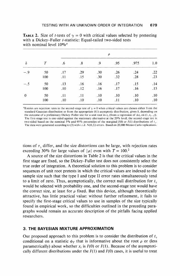
TABLE 2. Size of t-tests of ey = 0 with critical values selected by pretesting with a Dickey-Fuller t-statistic: Equal-tailed two-sided tests with nominal level 0lfoa

p

6 T .6 .8 .9 .95 .975 1.0

-.9 50 .17 .29 .30 .26 .24 .22 100 .11 .15 .30 .32 .28 .23

-.5 50 .13 .16 .16 .17 .15 .14 100 .10 .12 .16 .17 .16 .15

0 50 .11 .11 .10 .10 .10 .10 100 .10 .10 .10 .11 .10 .10

aEntries are rejection rates in the second-stage test of -y = 0 when critical values are chosen either from the standard Gaussian distribution or from the appropriate 1(1) asymptotic distribution, given 6, depending on the outcome of a preliminary Dickey-Fuller test for a unit root in xt (from a regression of Axt on (1,xt-1)). The first-stage test is one-sided against the stationary alternative at the 20% level; the second-stage test is two-sided based on the nominal 507% and 95%7o percentiles of the marginal I(0) or I(1) distributions of t'. The data were generated according to (3) with i.i.d. N(0, E) errors. Based on 20,000 Monte-Carlo replications.

tions of rT differ, and the size distortions can be large, with rejection rates exceeding 30% for large values of I p I even with T = 100.2

A source of the size distortions in Table 2 is that the critical values in the first stage are fixed, so the Dickey-Fuller test does not consistently select the true order of integration. A theoretical solution to this problem is to consider sequences of unit root pretests in which the critical values are indexed to the sample size such that the type I and type II error rates simultaneously tend to a limit of zero. Thus, asymptotically, the correct null distribution for t. would be selected with probability one, and the second-stage test would have the correct size, at least for p fixed. But this device, although theoretically attractive, has little practical value: without further refinement, it fails to specify the first-stage critical values to use in samples of the size typically found in empirical work, so the difficulties outlined in the preceding para- graphs would remain an accurate description of the pitfalls facing applied researchers.

3. THE BAYESIAN MIXTURE APPROXIMATION

Our proposed approach to this problem is to consider the distribution of tL conditional on a statistic OT that is informative about the root p or (less parametrically) about whether x, is I(0) or I(1). Because of the asymptotically different distributions under the I(1) and I(0) cases, it is useful to treat


the order of integration d as a dichotomous unknown parameter. Instead of performing a pretest on this unknown parameter, a Bayesian procedure is used to construct posterior probabilities for d given XT. This approach can be developed for general XT as long as these posterior probabilities can be computed. In this article, however, we focus on a specific class of OT statistics developed by Stock [30]. Before turning to the proposed Bayesian mixture procedure, we briefly review the construction and properties of these statistics. The theory for OT is set out for general detrending, although only the results for the demeaned case are used in the subsequent analysis of inference on y.

3.1. Construction of Posterior Probabilities for /(1) and 1(0)

The construction of the proposed approximation relies on a class of statistics OT = O(VT), introduced by Stock [30], that permit computing the posterior probability that x, is I(1) or I(O) when prior probabilities are placed solely on the point hypotheses I(1) and I(O), that is, without reference to a specific prior distribution over parametric representations of the x, process. (For an alternative approach see Phillips and Ploberger [25].) Write x, as

xt = dt + ut, (6)

where dc is deterministic and ut is stochastic. In the general case, the I(O) and I(1) hypotheses are taken to refer to properties of partial sums of ut. Let UOT(X) = T-1/2 ZVI T

us and U1T(X) = T 1/2U[TX], let 'yx(i) = cov(xt,xt-j) for a second-order stationary process xt. Throughout it is assumed that initial conditions have finite variance. The I(O) and I(1) models are respectively defined by:

00

I(O): UOT > WOW, where w 2 = E a(j), 0 < W2 < 0, (7) j=-00

I(1): UlT=>WIW,

where4D2= 2 V'U(f) 0<4<o (8) j=-00

The VT statistic is constructed by using detrended data xt. Let xt = xt- dt, where dt is an estimator of dt. Let VT(X) = cV1 T-12 X, [xi' where @ E m--ET k(MlfT) xd (Im |) and jxd(m) = T E t=m+-?1Xt t-m. The kernel k (*) is assumed to satisfy k (w) = O for I w I 1; k (w) = k (-w); 0 < k (w) ' 1 for I w < 1; k(O) = 1; and fe ,e=1 k(u/f) ?- Kfor all f > 1, whereK > O. It is assumed that the sequence of lag truncation parameters, 2T, satisfies f2 ln T/T --0, eT 0o. Let NT= T/EfT_Tk(m/fT). Let the trend estimation error be cI = dt- dt. Let IIztII = T' ZtT= z7 for a time series Zt, DOT(X) = T-1/2 ZT=LI ds, and DIT(X) = T1l2d[Tx]. The estimated trend is assumed to satisfy the following conditions.


Detrending Condition A. If u, is I(0), then

(i) (UOT,DOT) * &.0(W,DO), where Do E C[0,1], and (i 2 11 d7t 11 P 0.

Detrending Condition B. If u, is I(1), then

(i) (UIT,DIT) v 1(W,D1), where D1 E C[0,1], and (ii) 11 A di 11 = Op (1) .

The properties of specific functionals of VT under the I(1) and I(0) models for several detrending processes have been studied by Kwiatkowski et al. [12], Phillips [22], and Perron [18]. These results are extended to the general Detrending Conditions A and B in Stock [30, Theorem 1], where it is shown that if x, is I(0), then VT => Wo, whereas if xt is I(1), then NT-1/2 VT =:>

where Vd'(X) =foW Wd(s)ds/{f0 lWd (S)2 ds 12 , where Wod(s) = W(s)-DO (s) and Wld(s) = W(s) -D (s).

The general detrending conditions are satisfied by polynomial detrending by ordinary least squares (OLS) and by piecewise linear ("broken-trend") detrending. We will focus on the case of constants included in the regression so that a mean is subtracted from the data. Accordingly, denote the demeaned processes Wod and Wld by WJ' and WI, respectively, where Woy(s) = W(s) -

sW(l) and Wt'(s) = W(s) - f W(r)dr. These results permit computing the posteriors that xt is I(1) or I(0). Let

o(-) be a functional such that (i) o is a continuous mapping from D [0,1] (R1; (ii) /(ag) = ?(g) + 21na, where a is a scalar and g E D[0,1]; and (iii) Q(Wod) and O(Vrd), respectively, have continuous densities fo and f1 with support (-oo,oo). Let XT = O(VT); under these conditions, if xt is I(0), then XT O(WOg), whereas if xt is I(1), OT- lnNT O((Vd ) . The posterior probability that the series is I(d), given the statistic XT, iS p(I(d) I kT) = P(0T I(d))HId/p(T), where Hd = p(I(d)) is the prior probability that the process is I(d), d = 0, 1. In large samples, p (XT II(O)) and P (XT I(1)), respectively, can be approximated by fo (5T) and fi (4T - ln NT).

With these asymptotic approximations, the posterior probabilities can be computed as

p(I(O ) = = fo(,T)Ho (9a) P (OT)

p ((1) OT) = fl(kT lnNT)Hl (9b) P (kT)

A consequence of Theorems 1 and 2 in Stock [30] is that the posteriors asymptotically converge to zero or one: if 0 < Ho, H1 < 1 and if xt is I(0), then p (I(0) T) -+ 1 and p (I(l) I OT) + 0, whereas if xt is I(1), then p(I(O) IT) 4 0 and p(I(l) IkT)

P 1.


3.2. Bayes Mixture Approximation to the Distribution of tz

The consistency of the posteriors in (9) suggests their use for constructing the asymptotic approximation to the distribution of t,Y conditional on ?T specifically,

P (t-y I OT) = P (t-y I OT, d = O)p (I(O) |lOT) + P (ty I OT, d = I)p (IM1 |lXT) . (10)

As is made precise in Theorem 1, under (2), with -y = 0, the conditional distributions p ( t, I OT, d = 0) and p ( t, I OT, d = 1) asymptotically depend on only one nuisance parameter in the system in (2), 6, and so are readily computed.

The formulation in (10) has three parallel motivations. The first comes from its asymptotic properties. Because the posterior probabilities are consistent for zero or one, depending on d, p(t, OT) constructed by using (10) has the property that, for fixed p, the correct distribution for ta is used asymptotically.

The second motivation comes from recognizing (10) as a mixture of the I(O) and I(1) distributions with weights given by the posteriors p(I(d) I T); the greater the posterior weight on d = 1 for a realization of XT say, the greater the weight given to the d = 1 conditional distribution.

The third motivation comes from drawing an analogy between (10) and the Bayesian posterior distribution for -y. Suppose that we had available statistics Sp and S.,, where Sp is informative for p and (Sp, Se) are informative for -y. Let 0 denote the vector of nuisance parameters so that ('y, p, 0) comprise the complete parameter vector. From a Bayesian perspective, one might be interested in the posterior distribution of -y given (SP, S),

p(I I Sp s,) = f (Sp, s, Ie P, Op ( p a, dO dp/p(SP,S). (11)

Next make three assumptions: (i) the dependence of p(S,, Sp,y,p,0) on p reduces to whether p = 1 or IpI < 1, specifically, p(S ISp,y,p,0) =

p(S, I Sp,y,d = 1,0)1(p = 1) +p(SI I Sp, y,d=0,0)1(Ip I < 1); (ii)p(Sp |y,p,6) does not depend on 0 or -y, and depends on p only through p = 1 or p I < 1, specifically, p(S, Iy,O,p) =p(Sp d = 1)1(p = 1) +p(Sp d = 0)1(IpI < 1); and (iii) the priors on ey are flat and p (-y, p, 0) satisfies p (, p, 0) ocp (0)p (d = )6*(p - 1) +p(O)p(p)1(Ip < 1), where f p(0) dO = 1, 3*(.) is the Dirac

delta function, and fI pI<1p(p) dp = p(d = 0), where 0 ? p(d = 0) c 1 and p (d = 0) + p (d = 1) = 1. (An implication of Theorem 1 is that assumptions (i) and (ii) are satisfied asymptotically for (Sp, S7) = (OT, te).) With these assumptions, (11) simplifies to


p( IJ SP I SlS) {f p(SI I Sp,'y,d = O,6)p(f) d63 p(d = 0? Sp)

+ P (S71 Sp, y, d = 1, 6)p (O) d63 p(d = I Sp). (12)

Except for the integration over 0, if (Sp, Sy) = (T, ty), then the right- hand side of (12), evaluated at ty = 0, is the same as the right-hand side of (10) evaluated under the y = 0 null. This leads to the motivation of (10) as a large-sample approximation to the posterior in (12). For the system in (2), the dependence of the asymptotic approximation of p (S. I Sp,I y, d = O, 0) on 0 is limited to the single parameter &. Although in principle one could inte- grate over a prior on this parameter, in general prior beliefs about 6 are likely to be weak, and in any event 6 is consistently estimable, so in keeping with previous appeals to first-order asymptotic approximations, we treat a as known. The analogy between (12) and (10) would be more compelling were

(SP, S,) sufficient for (p, ,y), which (XT, tY) are not. For tractability, however, we restrict attention to the statistics (5r, ty-).

The value of (10) is that it provides an approximation to the conditional distribution of t,, which is readily computable, depends on only one nuisance parameter 6, and asymptotically delivers the correct null distribution of tL whether xt is I(0) or I(1) as determined by the fixed parameter p. These properties are implied by the following theorem.

THEOREM 1. Let (xt,yt) be generated according to (2) and let t. be the t-statistic that tests -y = 0 in (2) (with a constant included in the regression). Suppose that y = 0.

(a) If xt is I(O), then (i) (t-y, XT) * (ZO, ( WO)), where zo is a standard normal random variable

distributed independently of O(WO); and (ii) p(I(O) Io,) p 1 and p(I(l) I OT) ? 0.

(b) If xt is I(1), then (i) (te, XT-ln NT) (6fOl W'"(s) d W(s) /{ fO Wk,(S)2 dsJ 12 + (1 - 62)1/2Z

k(VP)), where V(X) = fox Wr(s)ds/Ifo Wtt(s)ds3 12 andzd isastandard normal random variable distributed independently of WI; and

( ii ) p (I I (O) T) O

and p (I (l1) I XT) 1 . Proof. All proofs are given in the Appendix.

Although the results in Theorem 1 are presented for x, generated according to (2a), in fact they apply more generally to x, satisfying either the I(0) or I(1) conditions in (7) and (8), of which the parametric model (2a) is a special case. In addition, the results are readily extended to more general deterministic terms than the constant considered here. For example, if x,


is linearly detrended by OLS, then Theorem 1 holds, except that WI, W0, and WI are replaced by their linearly detrended counterparts.

These results provide a straightforward mechanism for computing asymptotic approximations to the conditional distributions p (t, I V,, d = 0) and p (t, I XT, d - 1). In the I(0) case, t,, and XT are asymptotically independent, so this conditional distribution is simply a standard normal. In the I(1) case, the limiting conditional distribution is nonstandard but can be computed as p(te, T - ln NTI d = 1)/P(OT - ln NT| d = 1), where the joint distribution is computed by using the limiting representation in Theorem l(b). Despite the presence of nuisance parameters in (2), only the long-term correlation 6 between (1 - pL)x, and r,22 enters the asymptotic distributions of (ti,,T),

and then only in the I(1) case. The dependence of the joint limiting distribution of (tv, 9'T) on 6 means

that in practice 6 must be estimated to implement the Bayes mixture approximation in (10). However, this joint distribution is continuous in 6 and, moreover, 6 is a function of the spectral density matrix at frequency zero, Q, which in turn is consistently estimable (see, e.g., Andrews [1]). For the first-order asymptotic treatment here, we therefore treat 6 as known.

4. PERFORMANCE UNDER LOCAL-TO-I(1) AND LOCAL-TO-I(O) MODELS

One might suspect that the first-order asymptotic results of Section 3, which hinge on whether p is equal to or less than one, might provide poor approximations when x, is I(0) but p is large or, alternatively, when xt is I(1) with a large moving average root. This section provides some theoretical results for the case that xt is local to I(1) (I(0) with a large autoregressive root) or, alternatively, is local to I(0) (I(1) with a large moving average root). This is done by first examining the properties of the oT-based posteriors and decision rules when x, is local to either I(1) or I(0). Next, the performance of the Bayesian mixture approximation (10) is studied when xt is local to I(1).

4.1. First-Stage Posterior Probabilities Under Local-to-I(O) and Local-to-I(1) Models (General Detrending)

The results of this subsection are developed for general polynomial trends with OLS detrending; this contains the demeaning procedure considered in Section 3 as a special case. The trend component dc is given by

dt = zt', (13)

where Zt = (1, t, t2,. .t q), where the unknown parameters f are estimated by regressing xt onto Zt to obtain the OLS estimator f3 of S. Thus, q = 0 corresponds to subtracting from x, its sample mean and q = 1 corresponds to


linear detrending by OLS. For general q, under (13) the detrended data are xtd = xt -z z' = ut - d, where d-t = Zt (T=l Z/)' ETZI ZtUt.

The local-to-I(O) model considered here combines the I(0) model with the I(1) model, with a weight on the I(1) component that vanishes at rate T. Specifically, let

xt = d, + ut, ut = uot + HTult, (14)

where u0t and ult are, respectively, I(0) and I(1) as defined in (7) and (8) and where HT = h/T, where h is a constant. This representation has a natural interpretation as an unobserved components time series model in which the I(1) component is small relative to the I(0) component. Because of this analogy to unobserved components models, the two components here are taken to be independent, although the results below are readily extended to the case of a nonzero cross-spectrum between Ault and u0t.

The local components model can be rewritten as a moving average model in first differences where the largest MA root approaches one at the rate T. In the special case that Ault and uot are serially uncorrelated, the stochastic element in the local-to-I(O) model in (14) has the MA(1) representation Z Ut = 7t- OTt-l, where OT = 1 - (h?yu0(0)/'yU (0))/T + O(T-2).

The local-to-I(1) model is given by

xt = dt + ut, Ut = PTUt-I + Vt, where PT = I + c/T, (15)

where c is a constant and vt is I(0) with spectral density at frequency zero equal to 2rw2 (say). Under this local-to-I(1) specification, UIT(e) =

T-112UI[T.] converges to a diffusion process, that is, U1T * co, Bc, where BC(s) satisfies dB,(s) = cBc(s) ds + dW(s) with B,(0) = 0.

Theorem 2 summarizes the behavior of VT under these local processes with polynomial time trends of the form in (13) detrended by OLS. Because the local-to-I(0) specification is a combination of both I(0) and I(1) processes, we make the distinction between the limiting representations of these two processes, that is, in the I(0) case UOT => COO WO, whereas in the I(1) case UIT => WI W1, where W0 and WI are independent standard Brownian motions.

THEOREM 2. Let dc be given by (13) and detrending by OLS.

(a) if xt is local to I(O) as specified by (14), then VT = W0 r, where WOdr(X) Wod(X) + rfx Wd(s) ds, where r = hwl/c0o, Wd(X) = WO(X)-v(X)'M-'b, Wd(X) = WI(X) -(X)'M- 1f; M, v, and t are, respectively, (q + 1) x (q + 1), (q + 1) x 1, and (q + 1) x 1, with elements Mjj = 1/(i + j - 1), vi (X) = X'/i, and (i(X) = Xj, and 4, 'if are (q + 1) x 1 with (i = Wo(1) - (i- I)f'0si-2 Wo(s) ds, i =1 . q + and T = fJ 1 (s) WI (s) ds.

(b) If xt is local to I(1) as specified by (15), then NfT'2 VT => VP, where Vd(X) =

f"Bcd(s) dsl I fo&02 dr} I/2, where Bcd(X) = Bc (X)- (X)'M - 1 f (s)Bc(s) ds.

This theorem permits studying the posteriors under the local models. Con- sider the local-to-I(0) model. For functionals 0 discussed in Section 3A,


+(VT) =O (WO,r) = Op(1), sofo(4)(VT)) = Op(1) butf1 (4)(VT) - lnNT) + 0. For priors 0 < Ho, HI < 1, p(I(O) IjT) + 1 and p(I(l) I 4T) 2 0, that is, under the local-to-I(O) alternative, x, will be classified as I(O) with probability tending to one. Similarly, under the local-to-I(1) alternative, O(VT) -

lnNT= (Vc) = Op(l), so thatp(I(O) IT) 4 O andp(I(1) I T) 4 1 andxt will be classified as I(1) asymptotically.

It is instructive that this asymptotic misclassification of these local processes contrasts with the behavior of classical hypothesis tests based on 4)T

To be concrete, suppose that a one-sided test with asymptotic level a of the I(O) hypothesis is performed by rejecting if XT > Co, where c, is the upper 100(1 - a)th percentile of the distribution of 4)(Wd). Then the asymptotic probability of rejecting the local-to-I(O) alternative is Pr[O(WO r) > Cj.

Because O(Wo r) = Op(l) in general, this probability will exceed the level but will be less than one.3 Classical tests will have nontrivial-indeed, possibly high -power against these local-to-I(O) alternatives, but in large samples the Bayesian decision rules will classify them as I(O) with probability one for any nontrivial choice of priors. The same conclusions apply to the local- to-I(1) model for the same reasons: classical tests will have nontrivial power against this alternative, even though asymptotically the Bayesian decision rules will classify a local-to-I(1) process as I(1) with probability one.

This contrast with classical tests highlights the source of the asymptotic misclassification by this Bayesian procedure. Because the rate of convergence of 4(VT) differs by lnNT under the null and alternative hypotheses, one could perform classical hypothesis tests of (for example) the I(O) null against the I(1) alternative by using a sequence of critical values ca, T indexed to the sample size such that Ca,T -+ oo but that Ca,T - lnNT -+ -oo. If u, is truly I(O), the test would reject with asymptotic probability 0; but if u, is truly I(1), it would reject with unit asymptotic probability, so that this too would form a consistent classifier. Because O(VT) = Op(l) under the local-to-I(O) alternative, this classifier would also reject the local-to-I(O) model with probability zero asymptotically, although it would reject the local-to-I( 1) model with asymptotic probability one. The cost of eliminating the type I error is to introduce asymptotic misclassification in a vanishingly small neighborhood of the I(O) and I(1) models.

4.2. The Bayesian Mixture Approximation Under Local-to-I(1) Models

The results of Theorem 2 permit analyzing the distribution of t. for x, generated according to a local-to-I( 1) process, so that the largest root of x, is local- to-I( 1). Specifically, let p in (2a) be nested as p = 1 + c/T, where c is a constant, and let A, in (2a) be given by the sequence A,,T =-C( -o (1))-,I/T where AX is a constant. Asymptotic representations for the various statistics are given in the next theorem.


THEOREM 3. Suppose that (xt, yt) are generated according to (2) with p = 1 + c/T and that the null hypothesis Ho: -y = 0 is true. Then:

(a) (t-,0T_ In NT) * (6Xf0 B'(s) dW(s)/tft B'(s)2 dsj 1/2 + (i _62)1/2z -(v)

where Vl Ac(X) = JfOBu(s) ds/lfOl BIt(s)2 ds 1/2, zisastandard normal random variable distributed independently of (B j, W), and Bj = - flo Bc (s) ds, where Bc (s) satisfies dBc(s) = cBc (s) ds + d W(s).

(b) p(I(1) IT) + 1 and p(I(O) IkT) . 0.

The result (a) implies that the asymptotic joint distribution of (ti, OT),

and therefore the distribution of t-, given XT, is different when c * 0 than in the unit root case c = 0 (given in Theorem 1(b)). The result (b) implies that the local-to-I(1) process will be misclassified as I(1) with probability one, so that the mixture distribution in (10) will asymptotically place all weight on the I(1) conditional distribution. Taken together, these two results imply that, when p is local to one, the Bayesian mixture approximation will yield the incorrect asymptotic distribution. The magnitude of the resulting size distortions in local-to-I(1) models is investigated numerically in the Monte- Carlo analysis in Section 6.

5. POWER OF THE PROPOSED TESTS AGAINST LOCAL ALTERNATIVES

We turn to an investigation of the theoretical power properties of the test of e = 0 against a local sequence of _YT ? 0, performed by using the Bayesian mixture approximation in (10). As a simplification, the local power is analyzed for a special case of (1) in which only the first lag of x, and Yt enter the equation for x,. That is, (x,, yt) are assumed to be generated by

xt = ALx + pxt- I + /Yt- I + q I t (16a)

Yt = Iy + JTXt-I + n72t, (16b)

where Hx + flty = 0. Although there are no deterministic terms in (16), the statistics are computed by including a constant in both (16a) and (16b) to maintain comparability to the results in Section 2.

Because of the different orders in probability of xt, the local alternatives in the I(O) and I(1) cases differ: for some constant g,

If IPI < 1: YTy=g/Tl/2 (17)

If IPI = I yT = g/T. (18)

The asymptotic representations of the relevant statistics are summarized in the next theorem.


THEOREM 4. Suppose that (x,, Yt) are generated according to (16).

(a) If IpI < 1 and eT is given by (17), then (i) tY

= Z + [Yx(O)/22 l/2g, where z is a standard normal random variable; and

(ii) p(I(O) IkT) 1 and p(I(1) I XT) ? 0 (b) If p = 1 and 'YT is given by (18), then

(i) (te, - lnNT) =* (gfI2fflJ Bu(s)2ds/E22 12 + 6 fl Bg(s)dW(s)!/

[fC B (S)2 dS 1/2 + (1 _ 62)1/2Z, k(VUc)), where Vr c(X) = f B(s) ds/

{fO Bj(s) ds1'l2, Q = ElI + 213EI2 + E32E22, z isastandard normal random variable distributed independently of (B', W) and Bj = Bc(s) - fl Bc(s) ds, where Bc(s) satisfies dBc(s) = cBc(s) ds + d W(s) with c =

fg; and (ii) p(I(1)M T) P 1 andp(I(O) I T) ? 0-

The result in the p I < 1 case is conventional. Because the posterior probabilities asymptotically place all mass on the I(0) distribution, the local asymptotic power function for a two-sided level a test with Gaussian critical values ?ca/I2 is 4)(-Ca2 - gYex(o)/E22Jl/2) + 4(-C,/2 + g9Y(O)/E22J1/2),

where 4 is the cumulative normal distribution, the same local power function that would arise were it known a priori that I p I < 1, so that Gaussian critical values would be used at the outset for the ta test. In this sense, if I p I < 1, the use of the Bayesian mixture distribution results in no asymptotic loss in power of the second-stage test regardless of the priors nto and H,.

The results for the p = 1 case are more unusual and arise from the main- tained possibility of feedback from yt to xt, which results in xt being local to 1(1). This implies that the mixture distribution asymptotically places all weight on the I(1) conditional distribution. In addition, in this case yt is local-to-I(0). The results of Section 4 imply that a posterior odds ratio based on OT would, with high probability, classify Yt as I(0). Thus finite-sample evidence based on the OT classifier that yt is 1(0) does not imply that 'y = 0 but merely that -y is not too large.

For I 61 < 1 in the p = 1 case, the local asymptotic power function of the two-sided equal-tailed test of -y = 0 is given by

P [Reject Ho: -y = ? | OYT = g/T]

[ I C

_, 1/2 I

+ E4[) Cu, 1/2c$(6 + Tc + 1TH 1

(19)

where k = o(V c), Oc = Q11 fC B,(s)2ds/E221 12, H - If 1 Br(s) dW(s)1/

f1o B" (s)2 dsJ 1/2, and ce,a72(4) and Cu,a/2(k) are, respectively, the lower and upper I ath quantiles of the conditional distribution p ( t I OT = 0, d = 1). The difference between (19) and the local power function of the test based on tz when it is known a priori that x, is I(1) is that the critical values of the


latter test do not depend on XT, that is, the critical values in (19) are replaced by the constant critical values Cf, a/2 and Eu, a/2 taken from the marginal I(1) asymptotic distribution of t.. For 6 = 0, these two tests have the same critical values and thus the same local asymptotic power, but for 6 ? 0 their power functions will differ and must be compared numerically.

The local asymptotic power functions of these two tests - the proposed conditional test and the test based on t,, when p = 1 is known a priori-are plotted in Figure la for 6 = -.5 and in Figure lb for 6 = -.9, in both cases for ,B = 0 and S I = E22 (SO QII1/E22 = 1). Neither test dominates the other, although for most values of g the proposed test has higher power than the test based on the unconditional d = 1 critical values. If p = 1 is known a priori, then neither test based on te is optimal relative to the system likelihood ratio test, which imposes the p = 1 restriction. The power function of the system likelihood ratio test, computed for ,B = 0, is also plotted in Figure 1 (the short-dashed curve).4 For 6 =-.5, the power loss of the proposed procedure is moderate relative to the system likelihood ratio test; for 6 = -.9, it is substantial. In summary, if p = 1 and 161 is large, substantial power is lost by not imposing this restriction a priori; but if this restriction is not imposed and tests are based on the single equation (2b), the proposed procedure often outperforms the test based on the marginal I(1) null distribution of ty.

6. NUMERICAL ISSUES AND MONTE-CARLO RESULTS

6.1. The Specific VT Statistic and Numerical Issues

The specific OT statistic used here is one of the statistics studied in Stock [30]:

1(VT) = In{ VT(S)2ds} In =n{ T1 Z (xt,)2}. (20)

With some modifications, this statistic appears in different literatures vari- ously as a test for random coefficients (Nabeya and Tanaka [14]), as a test of the null of a unit MA root against an MA root less than one (Saikkonen and Luukkonen [27]), as test of the I(O) hypothesis against the I(1) alternative (Kwiatkowski et al. [12]), and as a test for breaks in deterministic trend components in an I(O) time series (Perron [18]), and it is also related to the Sargan-Bhargava [28] test of the unit root null. See Stock [30] and Perron [18] for further discussion.

All computations reported here place equal weight on the I(1) and I(O) hypotheses, that is, Hlo = I = 0.5. The spectral density of x, at frequency zero, w2, used to construct VT, was estimated by using a Parzen kernel with lag truncation parameter QT = min( 'T, 4max(T/10) 9), where eT is Andrews's [1] data-dependent estimated lag length for the AR(1) model for the Parzen kernel. (Note that eT satisfies the rate conditions for the asymptotic representations of VT.) For the results reported here, fmax was set to 10. Given


00 o.

0

t S ~~~~\\\ ,1

(N \ II

'16 -8 -4 0 4 8 12 16

9 (A) 6_-0.5

0

00

o i

0

010 -8 -4 0 4 8 1 2 1 6

9

(B) 6 = -0.9

FIGURE 1. Asymptotic power of tests of -y = 0 against the local alternative 'YT = g/T when XT iS I(1), ElI = E22, and ,B = 0 for (A) 6 = -.5 and (B) 6 = -.9. Solid line: Bayesian mixture approximation test; long-dashed line: test based on t,, by using the I(1) marginal null distribution of tr; short-dashed line: system likelihood ratio test that imposes p = 1.


priors -Io and Il1, the posteriors p(I() I T) and p(I(l) |T) were computed by using kernel density estimates of the asymptotic distributions fo and f1 for a given functional 4. For additional discussion, see Stock [30].

The conditional distributions of p(t1 | T, I(0)) and p (t7 | T, I ()) were computed by using the limiting representations in Theorem 1. In the I(0) case, the limiting conditional distribution is simply N(O, 1). In the I(1) case, t,, and XT-ln NT are asymptotically dependent random variables for 6 ? 0. The conditional distribution p (ty I 'kT = O, d = 1) for a value of 0 was computed by using a nearest-neighbor algorithm that was implemented by using 16,000 Monte-Carlo replications of (OT -lnNT, t), generated under the I(1) model with T = 400. The mixture distribution was computed by drawing randomly from the independent N(0, 1) I(0) distribution and this nearest- neighbor estimate of the I(1) conditional distribution.5

The quantiles of the mixture distribution p ( I |T = ) for the case HI =

JII, = 0.5, 6 = -0.9, and NT = 26.65 (corresponding to QT = 5 and T= 100 for the Parzen window) are plotted in Figure 2 as a function of 0. For low X, the posteriors place most weight on I(0), and the critical values are close to the N(0, 1) critical values. As 4 increases, more weight is placed on the I(1) distribution, and the critical values shift up sharply.

As discussed in Section 3, the mixture distribution depends on one nuisance parameter, the long-run correlation 8. In practice, 8 is unknown and would need to be estimated. As noted in Section 3, however, 6 can be estimated consistently whether xt is I(0) or I(1). In Monte-Carlo analysis, we therefore adopt the expedient of treating 6 as known. An extension for future research is to study the effect of estimating 6 on the finite sample performance of (10).

6.2. Monte-Carlo Results

The Monte-Carlo experiment studies the model examined in Section 2.2 for which the two naive procedures were found to work poorly. Specifically, the data were generated according to (3) with ELI = E22 = 1 and E12 = 6. The performance of the statistic XT is examined in Table 3, which reports the mean posterior probabilities from the first-stage estimation. These results support several of the theoretical predictions in the preceding sections. For p < 8, the posteriors tend to zero monotonically as T increases, so that the series are being correctly classified as I(0). For p = 1, the mean I(1) posterior increases to .899 for T = 400, again correctly classifying the series. The procedure has difficulty for large p when the mean I(1) posterior initially increases with T rather than decreases (p = .90, .95, and .975), although in each case for sufficiently large T the posteriors eventually decline.

Table 4 summarizes size results for the equal-tailed 100o-level test of 'y = 0 for various values of 6, p, and T by using the Bayes mixture approximation conditional critical values. For T = 100, the largest discrepancy is the size of


0

0

(n

0

0

0

0

0~~~~~~~~~~~ XTa coptdbXsn T ihaPre enl O-1. -0. 0. 0._ . . . .

s l IN , IN , 9 ( l a I ( l T f

in Section 2 indicates that conventional approaches to the choice of critical values for second-stage inference, by either ignoring unit root problems altogether or pretesting with a unit root test, can lead to substantial overrejec- tions when the null -y = 0 is true.

Second, the proposed Bayesian mixture approach has the desirable property that it asymptotically selects the correct 1(0) or I(1) distribution for fixed I(0) or I(1) models. The use of the first-stage statistic 4T has no effect on the local asymptotic power of the second-stage test if x, is I(0), and the numerical results of Section 5 indicate that the proposed procedure has bet-


TABLE 3. Mean posterior probabilities p (() I T) for first-stage inference I

p

T 0 .6 .8 .9 .95 .975 1.0

50 .089 .437 .471 .490 .489 .486 .488 100 .027 .334 .405 .514 .588 .629 .655 200 .006 .193 .262 .404 .576 .694 .815 400 .001 .102 .146 .261 .471 .675 .899

'The xt pseudorandom data were computed according to (3a) with the indicated value of p. The 'T functional used is given in (20). The process VT was computed by using demeaned data as described in Section 3.1. The Parzen kernel was used to estimate the spectral density with lag truncation parameter fT= min[fT, l0(T/100) 49], where eT is Andrews's [1] automatic lag truncation estimator (details are given in Section 6.1). For a given value of XkT, the posterior probabilities were computed by using a kernel density algorithm (based on 16,000 pseudorandom realizations of the limiting Brownian motion functional) described by Stock [30]. Prior probabilities are p(I(O)) = p(I(l)) = 0.5. Based on 5,000 Monte-Carlo replications.

ter power against most alternatives than the test of ey = 0 based on critical values from the marginal I(1) distribution of t.7

Third, the Monte-Carlo evidence is encouraging and suggests good size properties for two-sided tests based on these procedures for a wide range of values of p, including p close to, but less than, one. This is somewhat sur- prising because our theoretical results show that the size of the second-stage test will be incorrect, even asymptotically, when x, is local to I(1). For the )T statistic and models studied here, these initial results suggest that this

might not pose an important problem in practice. The results presented here suggest several directions for future research.

Throughout, we have treated the important nuisance parameter 6 as known. Although 6 can be estimated consistently, in finite samples its estimation pre- sumably will affect the performance of the proposed procedure and this remains to be investigated. The Monte-Carlo analysis has focused on a single 0 functional and uses only flat priors; the use of a different functional or informative priors might improve the finite sample performance. In addition, the performance of the second-stage statistic should be investigated for a wider range of x, processes than the AR(1) specifications considered here. More difficult is the extension to include additional potentially integrated and cointegrated variables in the second-stage regression. This increases the Bayesian selection procedure nontrivially and introduces additional nuisance parameters to the problem. The second of these difficulties has been examined by Toda and Phillips [33]. Finally, the extension to include additional lags of x, or Yt as regressors in the second-stage regression, although concep- tually straightforward, is of considerable practical importance because such


TABLE 4. Size of t-tests of ay = 0 with critical values computed by using the Bayesian mixture approximation (10): Nominal level 10%/o

p

6 T 0 .6 .8 .9 .95 .975 1.0

-0.9 50 .077 .057 .054 .057 .060 .070 .105 100 .093 .071 .072 .069 .068 .083 .168 200 .089 .075 .079 .093 .098 .094 .141 400 .102 .089 .091 .105 .135 .167 .160

-0.5 50 .101 .082 .085 .096 .101 .095 .119 100 .108 .087 .095 .088 .093 .095 .121 200 .093 .083 .094 .099 .096 .094 .110 400 .101 .098 .098 .110 .119 .122 .116

0.0 50 .106 .114 .110 .109 .122 .111 .115 100 .100 .105 .106 .106 .103 .108 .102 200 .101 .099 .107 .106 .097 .103 .103 400 .098 .105 .097 .103 .101 .105 .110

aThe data were generated according to (3). The first-stage 4T statistic was computed as described in the notes to Table 3. The critical values for ty (the t-statistic on xt- in the regression of y, onto (l,xt-1)) were computed as described in Section 6.1. Based on 5,000 Monte-Carlo replications.

lags are typically included in empirical practice. These and related problems are areas of ongoing research.

NO TES

1. The results in this paper complement those in Toda and Phillips [33], who considered the problem of sequential inference when some of the variables are cointegrated. Toda and Phil- lips's [33] theory maintains that the series are cointegrated, and they studied sequences of Wald tests of the null of no Granger causality in a vector autoregression, and inference is always x2. Their problem differs from the one considered here: our second-stage regression always examines a levels effect of the regressor, and the issue is whether standard or nonstandard distributions should be used to evaluate the significance of the estimated coefficient.

2. Similar results are obtained for a 10% pretest and a 10% equal-tailed second-stage test. For example, for T= 100 and 6 = -.9, if p = .9, the rejection rate is .34, whereas if p = .95, it is .27.

3. The nonstandard distribution of VT under the null and the alternative make it difficult to make general statements about the power function of such a test against the local alternative without resorting to numerical calculations. An illustrative case, however, is for the statistic k(VT) = ln(VT(1)2) in the case of no detrending. Under the I(O) null, this statistic has representation ln(W(1)2), which has a critical value of ln(x2a, where X?2;, is the a-level x 2

critical value. Under the local alternative, k(VT) = ln((WO(l) + rf WI (S) dS)2 }, which is distributed as the logarithm of (I + r2/3) times a standard x1. The power of this test of I(O) against the local-to-I(O) alternative is therefore Pr[X1 > X 2;ae/(1 + r2/3)]. This power function has its minimum at r = 0 and is monotone, increasing to one as r increases.


4. This power function is derived as follows. The Gaussian MLE for 'y in (16) with p = 1, f = 0, and an intercept in (16b) can be obtained by using the triangularized system, Ax, = , and y, = lA + -yxt, + KAXt + '2t, where K = E21lEII SO KAXt = Proj(ti2t7ii) and 2t =

ti2t - Proj(i2t tInI,); see Phillips [23], Saikkonen [26], and Stock and Watson [31]). Then ta is asymptotically N(0, 1) and the local asymptotic power against -YT = g/T is El 4b( -Ca/2 -

g(l - 62)-1/200) + '(-C,-,2 + g( - 62)-1/200)1, where 0o = Oc evaluated at c = 0 as defined following (19), and ca!2 is the 'Ca standard normal critical value. The power functions in Fig- ure 1 were computed by Monte-Carlo integration of the relevant expression (e.g., (19)) over ( C I ,A ) for c = 0 with 5,000 Monte-Carlo replications.

5. Specifically, 16,000 pseudorandom realizations from the limiting joint distribution were computed by using pseudodata that was generated from (2) with p = 1, ,8(L) = 0, & (L) = 0, 11I = F22 = 1, 12 = 6, and eT = 1. With the exception of 6, from Theorem 1(b) the choice of parameter values does not affect the asymptotic distribution of (1T - lnNT, t,). These can be interpreted as discretized approximations (discretized to 400 equispaced points) to the limiting Brownian motion functionals in Theorem 1(b). For a given value X, the mixture conditional distribution (10) was estimated by drawing K realizations, p (I(0) I 1kT = 1)K from a standard normal distribution and p(I(M) I T= =)K from the conditional distribution p(t, I = =k, d = 1); these latter p (I(1) I 1 T)K draws were computed as those t- for which the associated 1kT were the p (I(1) I 5t )K nearest neighbors of 1. Critical values of t,, given 1kT = 1k were computed by using the resulting Monte-Carlo mixture c.d.f. for a grid of X (grid size .05), which was then smoothed by Gaussian kernel regression to reduce Monte-Carlo error. Critical values for arbitrary 1 were computed by linear interpolation of the resulting table. These tables were constructed for various values of 6. The results reported here use K = 750.

REFERENCES

1. Andrews, D.W.K. Heteroskedasticity and autocorrelation consistent covariance matrix estimation. Econometrica 59 (1991): 817-858.

2. Bobkoski, M.J. Hypothesis Testing in Nonstationary Time Series. Ph.D. Dissertation, Uni- versity of Wisconsin, 1983.

3. Campbell, J.Y. A variance decomposition for stock returns. Economic Journal 101 (1991): 157-179.

4. Cavanagh, C. Roots Local to Unity. Harvard University, 1985. 5. Chan, N.H. On the parameter inference for nearly nonstationary time series. Journal of

the American Statistical Association 83 (1988): 857-862. 6. Chan, N.H. & C.Z. Wei. Asymptotic inference for nearly nonstationary AR(1) processes.

Annals of Statistics 15 (1987): 1050-1063. 7. Chan, N.H. & C.Z. Wei. Limiting distributions of least squares estimates of unstable auto-

regressive processes. Annals of Statistics 16 (1988): 367-401. 8. Dickey, D.A. & W.A. Fuller. Distribution of the estimators for autoregressive time series

with a unit root. Journal of the American Statistical Association 74 (1979): 427-431. 9. Fama, E.F. Efficient capital markets II. Journal of Finance 46 (1991): 1575-1617.

10. Fama, E.F. & K.R. French. Business conditions and expected returns on stocks and bonds. Journal of Financial Economics 25 (1989): 23-49.

11. Flavin, M.A. The adjustment of consumption to changing expectations about future income. Journal of Political Economy 89 (1981): 974-1009.

12. Kwiatkowski, D., P.C.B. Phillips, P. Schmidt & Y. Shin. Testing the null hypothesis of sta- tionarity against the alternative of a unit root: How sure are we that economic time series have a unit root? Journal of Econometrics 54 (1992): 159-178.

13. Mankiw, N.G. & M.D. Shapiro. Trends, random walks and tests of the permanent income hypothesis. Journal of Monetary Economics 16 (1985): 165-174.


14. Nabeya, S. & K. Tanaka. Asymptotic theory of a test for the constancy of regression coefficients against the random walk alternative. Annals of Statistics 16 (1988): 218-235.

15. Nabeya, S. & K. Tanaka. A general approach to the limiting distribution for estimators in time series regression with nonstable autoregressive errors. Econometrica 58 (1990): 145-163.

16. Park, J.Y. & P.C.B. Phillips. Statistical inference in regressions with integrated processes: Part I. Econometric Theory 4 (1988): 468-497.

17. Perron, P. The calculation of the limiting distribution of the least-squares estimator in a near-integrated model. Econometric Theory 5 (1989): 241-255.

18. Perron, P. A Test for Changes in a Polynomial Trend Function for a Dynamic Time Series. Princeton University, 1991.

19. Phillips, P.C.B. Understanding spurious regressions in econometrics. Journal of Economet- rics 33 (1986): 311-340.

20. Phillips, P.C.B. Toward a unified asymptotic theory for autoregression. Biometrika 74 (1987): 535-547.

21. Phillips, P.C.B. To criticize the critics: An objective Bayesian analysis of stochastic trends. Journal of Applied Econometrics 6 (1991): 333-364.

22. Phillips, P.C.B. Spectral regression for cointegrated time series. In W. Barnett, J. Powell & G. Tauchen (eds), Nonparametric and Semiparametric Methods in Econometrics and Sta- tistics, pp. 413-436. Cambridge University Press, Cambridge, UK. 1991.

23. Phillips, P.C.B. Optimal inference in cointegrated systems. Econometrica 59 (1991): 283-306. 24. Phillips, P.C.B. & S.N. Durlauf. Multiple time series regression with integrated processes.

Review of Economic Studies 53 (1986): 473-496. 25. Phillips, P.C.B. & W. Ploberger. Time Series Modeling with a Bayesian Frame of Refer-

ence: I. Concepts and Illustrations. Yale University, 1991. 26. Saikkonen, P. Asymptotically efficient estimation of cointegrating regressions. Economet-

ric Theory 7 (1991): 1-21. 27. Saikkonen, P. & R. Luukkonen. Testing for moving average unit root in autoregressive inte-

grated moving average models. Journal of the American Statistical Association 88 (1993): 596-601.

28. Sargan, J.D. & A. Bhargava. Testing for residuals from least squares regression for being generated by the Gaussian random walk. Econometrica 51 (1983): 153-174.

29. Sims, C.A., J.H. Stock & M.W. Watson. Inference in linear time series models with some unit roots. Econometrica 58 (1990): 113-144.

30. Stock, J.H. Deciding between I(1) and I(0). Journal of Econometrics, forthcoming. 31. Stock, J.H. & M.W. Watson. A simple estimator of cointegrating vectors in higher order

integrated systems. Econometrica 61 (1993): 783-820. 32. Stock, J.H. & K.D. West. Integrated regressors and tests of the permanent income hypoth-

esis. Journal of Monetary Economics 21 (1988): 85-96. 33. Toda, H.Y. & P.C.B. Phillips. Vector autoregression and causality. Econometrica 61 (1993):

1367-1394.

APPENDIX

Proof of Theorem 1. (a) First write xt in the form of (6). By assumption, (1 - a (L)L) is invertible, so under Ho, xt = (1 - a(I))-A, + (1 - a(L)L) -(-1It +

(L)q2t_) O= -, + v,, say. Because the roots of $3(L) are outside the unit circle and 77t is a martingale difference sequence, standard arguments imply that VT * WO. In


addition, tL has an N(0, 1) marginal distribution. To show the asymptotic independence of ty and kT, note that (1) is a special case of the system analyzed by Chan and Wei [7], so that their Theorem 2.2 implies (T-1'2 EST;] Z 7s, T-l E= l XI2s) (E'72B(.), ), where B is a standard bivariate Brownian motion, P is distributed N(0,E22yxY(0)) and where W(.) and P are independent. With this result, the asymptotic independence of tL, and XT follows by the consistency of 02 t22 (where t22 iS the OLS estimator of var(712t)), T-1 ZT-1 x1t l, and from writing VT(t) in terms of the partial sum process T- EST;] X5. Part (ii) follows from Stock [301.

(b) Write x, as xt = x0 + vt, where x0 is an initial condition and Avt = (1 - &(L)L)-1(-1It + 13(L)7n2t_1). Now vt is I(1) as defined in (8), so 7(VT) ' k(VO&) [30, Theorems 1 and 2]; this also follows, with minor modifications, from Kwiat- kowski et al. [12], Perron [18], and Phillips [22].

The joint representation of (OT, t) is obtained by using now-conventional frequency zero projection arguments. Note that T- 1/2 V[T.] = T- 1/2 Z[T.] As + op( l), where A = (1 - &())-1(7lt + 3(l)q2t), and that Q is the variance-covariance matrix of (t, 72t). Define W to be the limiting standard Brownian motion such that T-'/2 Lsi1' s Q W(I). In addition, decompose 2t as q2t = Proj(q2t I ~t) + 2t =

Q21 Q21 At + i22t, so that (<, ~2t) are a martingale difference sequence, and E( ttl2t) = 0 and var(i/2t)-- 822 = Q22 - ~Q1Ql2j . With this notation, te can be written:

Now, (T-'X2VIT T-'/2 z[I;' ~2s) (01K2 W(.),422fG(.)), where W(.) and G(.) are independent standard Brownian motions. In addition, 22 P 22 = Q22, SO

6fSW8(s) dW(s) (1 - ~2 )1/2fSwt(s) dG(s)

t'f 1 + 1 /2(A-l)

The argument in Phillips [23] or Saikkonen [26] imply that term in (A. 1) is independent of the first term and has an N(0, 1) marginal distribution, which leads to the representation given in the statement of the theorem. Part (ii) follows from Stock [30]. U

Proof of Theorem 2. Throughout, let TT = diag(1,T,.. Tq) and let MT =

T-' T ' EZT I ztz T-1. The nonstochastic q x q matrix MT has typical element MT,ij = T-' ETZ[ (t/T)i+i-2, which has the limit MT,ij - I/(i + j- 1) = Mij whether xt is I(0) or I(1).

(a) Let UT(X) = T- 1/2 E zTX7 ut, and let DT(X) =T- 1/2 E [TX dJ. The desired result will follow if it can be shown that (i) (UT,DT) satisfies detrending condition A(i), and (ii) &2 w o These are shown in turn.

(i) Bydirect calculation, UT= UOT+ THTUT, where UlT(X) =-' Z[TXI UlT(t/T). Because THT=h, UT= wO Wr, where W, (X) = W0 (X) + r WI (s) ds, where r= hwoI/cIo. Now, DT(X) = UT(X) MT rT, where PT(X) = T- [IT T lz5 and


rT= T- /2 ET 1 TTlztu,

= 4T + h'IT, where (IT

= T -/2 ET= IT lz,uot

and =T t=T l = jo TT(s)Uo T(s) ds, where T(X) = Ti'Z[TX].

From Stock's [30] Theorem 2 (OT,'IT,PVT,MT) > (c04), w 'I', v, M), where 4) is (q + 1) x 1 with 4?i = WO(l) - (i - I)fJs 2Wo(s)ds, i = 1,...,q + 1, 'I = fl (s) W1 (s) ds, where (j (X) = X'-1, and v is (q + 1) x 1 with vi (X) = X'/i, i = 1,. . . ,q + 1. Thus, FT * wo 0(4 + r'f) and DT(e) * coD(.), where D(X) = IJ(X)'M-1(4) + rI) . This verifies Detrending Condition A(i). Let XgT(x) = T

- X = UT(X) - DT(X), so that VT(X) =(c Xd (X).

Define Wod(X) = WO(X) - v(X)'M'4) and W(s) = W1(s) -(XM-1.

It follows that XOT(*) O WO r (*), where WO r (X) = Wo (X) + rfO W1 (s) ds -

v(X)'M-1(4) + rT) = Wod(X) - rfX Wd(s) ds, where the second equality uses V (X) = fox t(s) dS.

(ii) Let 32 = EIT Tk(M/fT)T-1 ZT-mi+ UtUtEm and c0 = > IT k(M/fT)

T-1 T= m I +I UOtUot_m . Now,

(t,2 - (;J < ' ( '12 - 'xo |<2_

eT T

= Z k(m/fT)T-1 Z [HTUitUit_1m1 + HT(UltUO,t_m1 M=-fT t= ml+l

+ UotUi,t-i mi)

eT T + Z k(m/fT)T-1 > tdtdt-1m, - (dtut-Hm + utdt-1m))

m=-fT t=iml+1

_ (2f + 1)1TH2jIT'1/2U1,tj + 2TI12HT IT-112U1tllll2llU t1ll2

+ (2QT + 1) ( 211ut 1/2 11dt 1 1/2 + 11dt AI 1. (A.2)

Because flT-'I2u1tI f W1(s)2ds, and 1 uotIi yu (jO), the first term in (A.2) P 0 if (2QT + I)TH2 -* 0 and (2QT + l)T1/ HT -- 0. These in turn follow from the rate condition f2 ln T/T--+ 0. Because u- uot I HT I Ui1I + 2HT I1 uot II2Il t I'2 A 0, || ut || P -yu(O), the second term in (A.2) P 0 if Q2TII A 0, which is Condition A(ii).

To show A(ii), write T IdTII = rTMT-IrT, from which it follows that

TIldTIl > W 2 (4 + r4I)'M-(4) + rI). This result and the rate condition T2 ln T/T -O 0 together imply that Q2I I T P 0, thereby verifying A(ii) so

that both terms in (A.2) P 0. Because co A wo, it follows that w2 A 00. Thus VT (X ) = r-1XT (X) > Wodr(*), the desired result.

(b) It is first demonstrated that Conditions B(i) and B(ii) hold for ut given by (15). Concerning Condition B(i), write DIT(X) = (T(X)'MTF4'T, where the terms are defined in the proof of part (a). Now, (QT,MT,IT) Q (S,M,coI), where t = fJOl(s)B,(s)ds. Thus, D1T(-) w w1 D, (.), where D1(X) = (X)'M'4', which verifies B(i). Let XdT(X) = T-2 X[TX] = UIT(X) - DIT(X), so that VT(X) =

O1f f0XXdT(s) ds. It follows that XdT(e) c w1Bgd(.), where B d(X) = BC (X) t())'M -' fOl t(s) Bc (s) ds.

Condition B(ii) follows from writing IIT'f2AdoII = foST(X)d where ST(X) =

TMf1` j(X)ST(X)'MT T' where ZT(X) = T XT 1zrTxj. Direct calculation shows


that ST=* S, where S(X) = w2I'M'- I(X) -(X)'M'4M , where S-(X) = (0,1,2X,

,q q- ), so 11JAd, 11 P 0, thereby verifying B(ii).

Next write NT 12 VT(X) = BT 1/2AT(X), where AT (X) = T-32 I X and BT-

T- EMT=_ kT(m/MT) (ImI)/Zr--CTk(m/lT). Now AT(X) w1fiBd(s)ds. To show that BT has the desired limit, it remains only to show that BT -T2 T T-1 (Xt')2 P

0. This was shown in Stock's [301 Lemma A. 1 when ut is I(1). The only part of the

proof of that lemma that requires modification for the local-to-I( 1) case is demon-

strating that the term D3T (as defined in that proof) P 0. From (A. 1) in Stock [30],

D3T P 0 if 1AJt 11 -P 0 (just shown) and if 11 Aut = OP (1). This final relation is now shown. Because (1 - PTL)Ut = Vt,

fAUt,J - VtJI = ||Vt + (PT - l)Ut-.I t- ||vtI

' 2PT - I IjUt1 1112j1vt 1 1/2 + (PT- 1)2 11Ut4.

Now (PT-1)2 IlUtI = C2T-frO UIT(S)2dS P 0 and 1I Pt 11 P

yU (0) by assumption. Thus, 11 AutJl -* -yv(O), so D3T -P+ 0 and Lemma A.1 in Stock [30] holds, thereby com-

pleting the proof. U

Proof of Theorem 3. (a) Under the stated assumptions, algebraic manipulations per-

mit rewriting xt as x, = ft + vt plus initial conditions, where ft is constant and vt satisfies

(1 - pL)(l - &(L)L)v, = f3(L)(yt,1 - nty) + ,It, where vo = 0. Thus, T7/2V[T.I =

T-(I2 [T1] p1TLI-S(l-&(L)L)-1( qlt + 3(L)iq2t-l) = T'12 S[T.11 p[T.)ss + op(l), where ~t = (1 - &( lO) (71 t + (M1)X2,)d. Note that ( t,q2t is a martingale difference

sequence with variance-covariance matrix U. As in the proof of Theorem 1(b), let

fl2t = fl2t - (Q21/Ql1)t. Then (T-1/2 [T--]P T_1/2 [T1 N2) * (91/2B (.)

221/2G (.)), where dBc(s) = cBc (s) ds + d W(s) and G is a standard Brownian motion distributed independently of W. The argument leading to (A. 1), applied here, yields,

6 fBs(s) d W(s) (1 _ 62)1/2 jB (s) dG (s) +~~~~~~~

t'Y 1/2 + 1/2 (A.3)

(fBS(S)2ds)B2 (fB(s)2ds)

As in (A. 1), the independence of G and (W, Bc, Br), and the N(0, 1) distribution of

the second term in (A.3) conditional on Bc yield the representation given in the state-

ment of the theorem. (b) It was shown in the proof of (a) that xt has the local-to-I( 1)

representation (15), so the results of Theorem 2(b) apply. The consistency of the pos-

terior probabilities follows according to the remarks following the statement of Theo-

rem 2. U

Proof of Theorem 4. Substitute (16b) into (16a) to obtain (1 - pL - 1YTL2)xt =

v,, where v, = -t + 0772t-1I (a) (i) For T sufficiently large, if I p I < 1, then for any finite g the roots of (1 -

pL - IYTL 2) will both be outside the unit circle, so that x, is I(0) in the sense of (7) and in particular T` r (xt1)2 P yx(O). Thus, under the local nesting in (17),

tV= t Et=I Xt_I ( YTXt-l + 2t,)3/{ E1 (xi' 1)- 221 3-=g[T- t-1 (x=t-1 )t/222312 +

IT T I (Xt- )2 I2/2 /2 + Z, the stated result. (ii) Because xt is I(0) in the sense of (7) for T sufficiently large, the results of Stock


[301 apply and, for the reasons discussed in Section 3. 1, the posteriors are consistent as stated.

(b)(i) When p = 1, (1 - pL - frYTL2) can be factored, (1 - r,L)( -r2L), where r, = 1 + VT and r2 = -VT, where VT - 2(l + 4I7T)1/2 - 1}. Let Tt =

(1 - VTL) (-qlt + 03t2t-1). Then, with xo 0, T-172XT.1 = T-' 2ZI (1 +

VT) [T , S`TS. Now VT = 3g/T + O(T 2), so T- 1/2 (1 + VT).1sT,-

T-1/2 E[; explog([T.] - s)/TI A P 0, where = mlt + 13t2t. Thus T-1/2X[T}

EII2B,(.), where B, is defined in the statement of the theorem, and where W is defined by T-1/2 T; ? > 1/2 W

To obtain the representation for t., note that Q is the covariance matrix of (~t, r2t) and write t =g{T 2 ET (t)2 21/2 + IT-' E~iTit2,/ 2 ETI (At1)2 1/f2. wrt t=gl t= l (X 0f_ 2/ t22 I T1Et Xt4 1712 ]/t T Lt= l t-1)2

The first term has the limit g{I 1 fo B j(s)2ds/l22} 1/2, where Ql1 = El, + 203I2 + 32E22. The behavior of the second term is the same as in Theorem 3(a). By combin-

ing this result for the first term with (A.3), we have

g f 1()2d1 1/2 6 B(s) dW(s) (i - 62)1/2 BA (s) dG (s)

te g 1/2 / 1/2

)Bc"(s )2ds) T(B"(S)2dS)

(A.4)

As in Theorem 3, G is distributed independently of (Bj, W), so the final term in (A.4) has a standard normal distribution and is independent of the other terms, which yields the representation stated in the theorem. (ii) It was shown in the proof of b(i) that xt is local-to-I(1), so the results of Theorem 2(b) apply and

p(I(M) IT) A Iandp(I(O) I T) O. U

inference in time series regression when the order...

Documents