centre for development, environment and policy p545 ... normal linear regression model. • to show...

C05

© SOAS CeDEP 1

Centre for Development, Environment and Policy

P545

Applied Econometrics

Prepared by Adam Prakash This module is partially based on the earlier module ‘Applied Econometrics for the Agricultural and Food Sector’ prepared for the University of London’s External Programme by Alison Burrell. Updated by Laure Latruffe in 2010, 2011 © SOAS | 3736

P545 Applied Econometrics Module Introduction

© SOAS CeDEP 2

MODULE INTRODUCTION

ABOUT THIS MODULE

• This module is about econometric methods and how they are applied to estimate and test the unknown parameters of economic relationships. Priority is given to both the statistical reasoning underlying the methodology and the practical considerations involved in using this methodology with a variety of models and real data.

• The focus of the module is on the classical linear regression model. This is the basis for much econometric methodology and it provides the framework for organising the module.

• The module covers

− the principles of regression analysis and its statistical foundations

− the simple linear regression model

− the multiple linear regression model

− departures from the assumptions of classical linear regression

− modelling economic behaviour

• There is a limit to the distance that can be covered in the study time available.

In an econometrics module, the trade-off between breadth and depth is low since, without good groundwork and sufficient information at each stage, ideas may be misunderstood and techniques misapplied. This module follows the standard itinerary of most econometrics textbooks. It deals only with single-equation models, but by the end of the module the student is ready to tackle simultaneous equation models, which would be the next stop-over on this itinerary.

• The practical exercises designed to be done with the help of the free computer software package R are an important element of the module.


© SOAS CeDEP 3

WHAT YOU WILL LEARN

Module Aims The specific aims of the module are:

• To explain the principles of econometric estimation and its statistical foundations.

• To present the theory of the classical linear regression model and explain why the conditions in such a model provide an ideal environment for ordinary least squares regression.

• To explain the procedures of interval estimation and hypothesis testing in the classical normal linear regression model.

• To show how econometric models can be made more realistic through the use of dummy variables and a dynamic specification.

• To explain how linear restrictions can be imposed on parameters during estimation and how these restrictions can be tested.

• To investigate the consequences of heteroscedasticity and autocorrelation of the disturbances of a regression model.

• To encourage an appreciation of what constitutes a `good' econometric model, and how to test that a model is well specified.

• To develop practical skills of data analysis, use of regression techniques and interpretation of regression results.

Module Learning Outcomes By the end of this module, students should be able to:

• understand and selectively and critically apply the basic principles of regression analysis and statistical inference in the context of a single-equation regression model

• formulate a single-equation regression model, estimate its parameters, carry out a variety of tests relating to model specification and critically interpret all results

• test hypotheses about economic behaviour and critically interpret the results of these tests

• specify and interpret models using dummy variables, different types of dynamic specification and incorporate and test linear restrictions

• test for heteroscedasticity and autocorrelation of the disturbances of a regression model, and take appropriate action when these conditions are found to be present based on critical interpretation.


© SOAS CeDEP 4

STUDY MATERIALS

The single textbook for the module is:

Gujarati D, Porter D (2010) The Essentials of Econometrics, 4th edn. McGraw-Hill.

This book has been chosen for this self-study module because of its attention to full explanations of concepts and procedures, its long introductory section presenting the basic statistical concepts used in regression modelling, and its avoidance of unnecessary algebra and difficult notation. At least part of every chapter is required reading for the module, and you are also encouraged to read those parts that are not specifically identified in the module texts, since all the material here should be within your grasp and will reinforce your understanding of the subject. By the end of the module, you will know this textbook well and will be ready for other more advanced readings.

Each unit in the study guide follows the same format and we will say more about the reasons for choosing their format in Unit 1. Each unit starts with a section on ideas and issues where the main ideas of the unit are explained in a relatively non-technical way. This is followed by a study guide section which takes you through the relevant parts of the textbook, commenting on and reinforcing the material. Next, there is a section (except in Unit 6 and in Unit 10) containing one or more worked examples in which various techniques and their application and interpretation are illustrated in the context of a practical modelling exercise. These examples are an important tool for learning: follow them through carefully, and later on, when doing the exercises, take care not to skip the question that asks you to reproduce the results of the worked example yourself. The worked example is followed by a set of questions whose answers are contained at the end of each unit and a summary of the material in the unit. Last but by no means least, each unit (except Unit 6 and Unit 10) also has a R guide explaining any new computer commands and procedures that are necessary for answering the questions in that unit.

The R guide of Unit 1 explains how to install and get started with this free software.

When studying each unit, we suggest that you study the text at your own pace and then work through the first few unit questions which are always designed to test your basic understanding of the unit material. If these questions reveal some weak spots, refresh them first before going on to the applied, data-based questions which you will need to answer in conjunction with the R Guide. When you have finished the questions and checked your answers, you should make a note of any additional knowledge or insights you have gained by doing the questions that you missed when studying the module text. The summary at the end of each unit briefly describes the topics covered and lists what you should have learnt through your study.


© SOAS CeDEP 5

Applied statistics and econometrics are subjects with a great deal of specialised jargon. It can be disconcerting to be faced with a number of unfamiliar new terms, many of them quite long and often rather similar to each other. We recommend very strongly that, right from the beginning of the module, you keep a glossary in which you list each new term as you encounter it, together with an explanation of the term in your own words. You should read through this glossary every few weeks, updating your definitions if you find that, as the module progresses, your understanding of the term develops along with your familiarity with the concept. A space is provided at the back of the study guide for your glossary.


© SOAS CeDEP 6

FURTHER READING

Intermediate textbooks

Greene W (2000) Econometric Analysis, 4th edn. Prentice Hall, New Jersey.

Gujarati D (1979) Basic Econometrics. McGraw-Hill, Singapore.

Judge GG, Hill CR, Griffiths WE, Lütkepohl H, Lee T-C (1982) Introduction to the Theory and Practice of Econometrics. John Wiley, Chichester.

Koutsoyiannis A (1973) Theory of Econometrics. Harper & Row, New York.

Advanced textbooks

Johnston J (1984) Econometric Methods, 3rd edn. McGraw-Hill, Singapore.

Maddala GS (1992) Introduction to Econometrics, 2nd edn. Macmillan, New York.

Other

Kennedy P (1985) Guide to Econometrics, 2nd edn. Blackwell, Oxford.

Helpful background reading about econometric methodology.

Hallam D (1990) Econometric Modelling of Agricultural Commodity Markets. Routledge, London.

Discussion of econometric modelling in agricultural economics.

Charemza WW, Deadman DF (1992) New Directions in Econometric Practice. Edward Elgar, Cheltenham.

Useful introduction to cointegration analysis.


© SOAS CeDEP 7

STUDY METHODS

Remember that people learn in different ways (and at different speeds). The units of the module follow a logical progression in setting out and elaborating the principles of the subject, but you can move about between units and topics if this suits you.

There is no single rule about how best to learn the kind of material presented in this study guide. Perhaps the best thing to do at the very beginning is to flick through the materials, picking out what is most interesting to you, noting what seems more difficult and what seems easier. You will notice that the module is activity-intensive. There are many questions and exercises to help you acquire the necessary analytical skills. Answers to questions and exercises are provided at the end of each relevant unit. Try to answer them on your own first before consulting the answers we have provided!

The wealth of material means that it is necessary to pace yourself through it. The Indicative Study Calendar at the end of this introduction gives you guidance on this and a series of study tips are included below, which may give you some hints on how best to study the module material.

Learning is an iterative process. It is often useful to go back to something studied earlier. It is always important to be clear about the aims and objectives of a particular unit. What are you trying to achieve in completing the unit; what are you expected to accomplish?

Reading and note taking

A key function of the units is to facilitate the activity of reading and learning. They highlight key points from the assigned readings, pose questions and provide a means of reinforcing, relating and applying the issues discussed in the readings.

In note taking, the activity of selecting what you think is most important, interesting and relevant, and putting it into your own words, is a powerful means of acquiring and developing a sound knowledge of the subject. As you read you should simultaneously be

• thinking about the content

• making notes where appropriate

• relating ideas and concepts

• comparing information with your existing knowledge

• considering the applications of what you are studying

Notes should be well organised and well structured (ie making use of headings, indentations etc), and clearly convey the meaning of what they refer to. You should always reference the notes to the relevant section or chapter; this will make it easier to return to the relevant reading for clarification and so on. You may find it useful to annotate the unit text and/or readings with connecting thoughts and ideas. This will help to link the elements of the module.

There are some features in the text of each unit that invite you to take some specific action before reading further:


© SOAS CeDEP 8

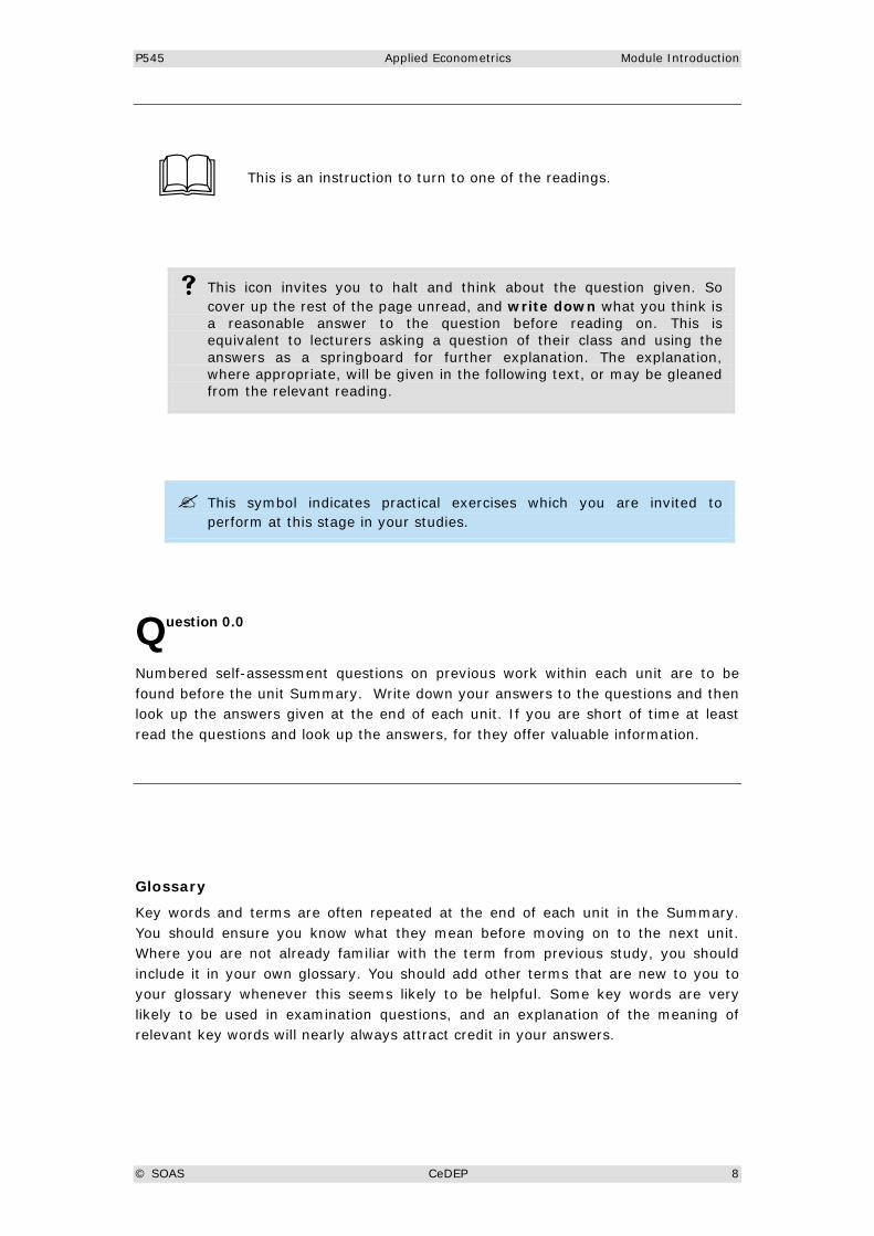
This is an instruction to turn to one of the readings.

This icon invites you to halt and think about the question given. So cover up the rest of the page unread, and write down what you think is a reasonable answer to the question before reading on. This is equivalent to lecturers asking a question of their class and using the answers as a springboard for further explanation. The explanation, where appropriate, will be given in the following text, or may be gleaned from the relevant reading.

This symbol indicates practical exercises which you are invited to perform at this stage in your studies.

uestion 0.0

Numbered self-assessment questions on previous work within each unit are to be found before the unit Summary. Write down your answers to the questions and then look up the answers given at the end of each unit. If you are short of time at least read the questions and look up the answers, for they offer valuable information.

Glossary

Key words and terms are often repeated at the end of each unit in the Summary. You should ensure you know what they mean before moving on to the next unit. Where you are not already familiar with the term from previous study, you should include it in your own glossary. You should add other terms that are new to you to your glossary whenever this seems likely to be helpful. Some key words are very likely to be used in examination questions, and an explanation of the meaning of relevant key words will nearly always attract credit in your answers.

Q


© SOAS CeDEP 9

TUTORIAL SUPPORT

There are two opportunities for receiving support from tutors during your study, and you are strongly advised to take advantage of both. These opportunities involve

(i) participating in the virtual learning environment (VLE)

(ii) completing the examined assignment (EA)

Virtual learning environment (VLE)

The virtual learning environment provides an opportunity, through the internet, for you to interact with both other students and tutors. A ‘Discussion Module’ area is provided through which you can post questions regarding any study topic that you have difficulty with, or for which you require further clarification. You can also discuss more general issues that are central or topical for your module or degree.

Additional features of the VLE include a technical area if you have any access problems, an administrative area for any relevant queries and profile areas where students and staff may introduce themselves. A very popular feature is the student ‘café’ where students may socialise and interact regarding any issue they choose (tutors are not allowed entry).


© SOAS CeDEP 10

ASSESSMENT

This module is assessed by:

• an examined assignment (EA) worth 20%

• a written examination in October worth 80%

Since the EA is an element of the formal examination process, please note the following:

(a) The EA questions and submission date will be available on the Virtual Learning Environment.

(b) The EA is submitted by uploading it to the Virtual Learning Environment.

(c) The EA is marked by the module tutor and students will receive a percentage mark and feedback.

(d) Answers submitted must be entirely the student’s own work and not a product of collaboration. For this reason, the Virtual Learning Environment is not an appropriate forum for queries about the EA.

(e) Plagiarism is a breach of regulations. To ensure compliance with the specific University of London regulations, all students are advised to read the guidelines on referencing the work of other people. For more detailed information, see the User Resource Section of the Virtual Learning Environment.


© SOAS CeDEP 11

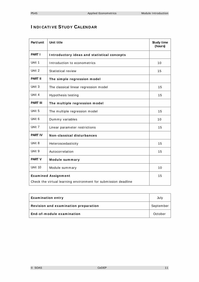
INDICATIVE STUDY CALENDAR

Part/unit Unit title Study time (hours)

PART I Introductory ideas and statistical concepts

Unit 1 Introduction to econometrics 10

Unit 2 Statistical review 15

PART II The simple regression model

Unit 3 The classical linear regression model 15

Unit 4 Hypothesis testing 15

PART III The multiple regression model

Unit 5 The multiple regression model 15

Unit 6 Dummy variables 10

Unit 7 Linear parameter restrictions 15

PART IV Non-classical disturbances

Unit 8 Heteroscedasticity 15

Unit 9 Autocorrelation 15

PART V Module summary

Unit 10 Module summary 10

Examined Assignment

Check the virtual learning environment for submission deadline

15

Examination entry July

Revision and examination preparation September

End-of-module examination October

Unit One: Introduction to Econometrics

Unit Information 1

Unit Overview 1 Unit Aims 1 Unit Learning Outcomes 1

1.0 What is econometrics? 2

2.0 Structure of module texts 6

3.0 Ideas: the concept of regression 8

4.0 Study guide 14

5.0 An example: the Keynesian consumption function 16

Self Assessment Questions 19

Unit Summary 21

Answers to Self Assessment Questions 23

P545 Applied Econometrics Unit 1

© SOAS CeDEP 1

UNIT INFORMATION

Unit Overview This unit introduces you to the study of econometrics. It begins by defining econometrics and then explains how econometrics relates to and differs from other branches of economics. The important roles of economic theory and data in econometric work are emphasised. Regression analysis is identified as the basis of econometric procedure. The aims and purpose of regression analysis are explained. The main steps of a typical econometric investigation are described and illustrated with an example.

Unit Aims • To define the nature and scope of econometrics

• To identify the special characteristics of econometrics as a tool of applied economics

• To describe and illustrate the main steps of an econometric investigation

• To identify some characteristics of economic data

• To practise some basic techniques of data investigation

Unit Learning Outcomes By the end of this unit, students should:

• have an appreciation of econometrics as a method of empirical investigation

• have an understanding of four major differences between econometric models and economic models

• have an understanding of the seven main steps of an econometric investigation

• have a knowledge of essential terminology relating to regression analysis

• know how to perform basic data analysis in R


© SOAS CeDEP 2

1.0 WHAT IS ECONOMETRICS?

Welcome to this module. Its aim is to give you an introduction to econometric methods or, more specifically, to linear regression which is the main statistical foundation for econometric work. Throughout the module you will be working with data; we hope you will find this interesting.

Economic theory is concerned with relationships between variables. You have already met some of these, including demand and supply functions for agricultural products, production functions, labour supply and demand functions, and so on. Economic theory aims to explain economic behaviour; this involves studying the relationship between economic variables and the factors that influence them.

The purpose of econometrics is to quantify economic relationships. Econometrics can provide numerical estimates of the parameters of these relationships and a framework for testing hypotheses about them. Broadly defined, econometrics is

‘ … the application of statistical and mathematical methods to the analysis of economic data, with a purpose of giving empirical content to economic theories and verifying them or refuting them…’

Source: Maddala GS (1988) Introduction to Econometrics. Macmillan, New York, Chapter 1

Other definitions are possible: in your textbook you will come across a number of definitions that each has a slightly different emphasis. Common to all definitions, however, is the stress on the empirical nature of econometric work.

• The process of econometrics involves the confrontation between economic theory and economic data in quantifying economic relationships.

Econometrics is not just a branch of mathematical economics. Mathematical economics need not have any empirical content at all whereas in econometrics the emphasis is on empirical analysis. At the same time, econometrics is not just a ‘box of tools’ to work with data. It requires, undoubtedly, a good training in statistical techniques but these techniques need to be deployed in an interactive process between theory and the data.

This module can be studied in its own right, but normally we would expect you to take it as part of the MSc programme where, in Part I, you will have studied various economic theories and models. You should therefore be familiar with a range of questions raised in theoretical discussions and with the results of some applied empirical studies. These are good foundations on which to build the study of econometrics. If up to now you have approached empirical studies from the point of view of theory or the consequences for policy making, we now invite you to look at them from the point of view of an econometrician. What is the difference?

To give empirical content to economic theories, the econometrician is confronted with four problems that hardly concern the economic theorist.


© SOAS CeDEP 3

Non-experimental data

Economic theory develops models using a priori reasoning applied to relatively simple assumptions. This procedure involves abstracting from secondary complications by assuming that ‘other things remain equal’ (or ceteris paribus), in order to investigate the links between a few key economic variables.

For example, in demand theory we say that the quantity demanded of a commodity (that is not a Giffen good) will fall if its price rises, other things being equal. These ‘other things’ which we assume are held constant include consumers’ incomes and income distribution, and the prices of substitutes and complementary goods.

This method is fruitful in economic theory but, unfortunately, it is rarely possible to carry out controlled experiments to test such statements. Therefore, in empirical economics the scope for observing such behaviour is severely limited. A researcher cannot alter a commodity’s price, holding other things constant, in order to see what happens to its demand.

In general, economic data are not the outcome of experiments but rather are observed and recorded in a non-experimental world where other things are never equal. Therefore, econometrics involves untangling the effects of different factors that act simultaneously rather than analysing the results of a laboratory experiment.

Stochastic relationships

Economic theory usually involves deterministic relationships between economic variables. This can be explained with a simple example: the Keynesian consumption function. In economic theory we assume that, if we know the level of aggregate real income, consumption will be uniquely determined. That is, for each value of aggregate real income there corresponds a given level of aggregate consumption.

In reality, however, we do not expect theoretical relationships to hold exactly. Even when all the main factors that systematically affect the behaviour of an economic variable are taken into account, there will still be some random variation due to non-systematic, ‘one-off’ factors and human variability.

Hence, in econometric work we deal with relationships between variables that contain a random or stochastic element, and that are therefore not deterministic in nature. We investigate functions between variables which we believe to be reasonably stable on average, but there is always a degree of uncertainty about them.

In econometrics we make explicit assumptions about these random components, called disturbances. This is why econometrics draws heavily on probability theory and statistical inference.

Observed variables

In economic theory we work with theoretical variables. Econometrics, in contrast, deals with observed data.

Obviously, there is a certain correspondence between them: data collection is inspired by some theoretical framework. For example, the framework for measuring national income account data derives from Keynesian economics, which is centred on the analysis of theoretical aggregates such as output, demand, employment and the price level.


© SOAS CeDEP 4

However, observed variables do not fully correspond to their theoretical counterparts because of differences in definition and coverage, and errors in measurement. For example, the ‘price level’ is an abstract concept that is usually represented empirically by some aggregate price index; however, the values it takes depend on the goods whose prices are covered by the index and the method of calculating the index.

Another example concerns modelling technology. In agricultural supply functions, the ‘state of technology’ is an important variable: changes in supply over time are driven both by price changes and by the pace of technological change. But how can technological development be measured? Many researchers resort to a simple time trend to represent this important variable.

Finally, ‘management’ is a key input in the theoretical specification of an agricultural production function but one that is always difficult to measure empirically: econometricians sometimes resort to proxy variables for management like the number of years of education the farmer has received but more often they omit this variable altogether in applied work.

In econometrics we need to be aware of the discrepancy between theoretical concepts and observed data, and its implications when quantifying theoretical propositions.

The treatment of time

The econometrician must make explicit assumptions about the role of time in his model. When economic theory postulates that consumption depends on disposable income, ceteris paribus, it implies that when income takes different values so too does consumption. Econometrics can quantify this dependency by using information about how consumption changes as income takes different values. However, this dependency could be observed empirically in two alternative ways:

(1) by recording how consumption and income move together over time, or

(2) by recording the consumption of households at different income levels during the same time period

In the first case, we have a time-series model, requiring time-series data (measured at intervals over time).

In the second case, we have a cross-section model, requiring cross-section data (measured for different individuals or micro-units at the same point or during the same period in time). The choice between a time-series and a cross-section model often depends on data availability, although this choice is less straightforward than it may seem.

First, we may need to modify our theory for explaining consumption changes over time before it can be applied to cross-sectional consumption analysis.

Second, there may be data considerations; for example, a time-series approach is hardly appropriate for studying how consumption varies with income during periods in which there has been virtually zero income growth.


© SOAS CeDEP 5

These four elements give econometric work its distinctive flavour:

• the fact that we cannot hold other things constant in empirical analysis

• the stochastic nature of relationships between variables

• the discrepancies between theoretical variables and observed data

• the need to make explicit assumptions about time

We cannot move straight from an economic model as formulated by economic theory to parameter estimation without dealing with these issues. In empirical analysis, our data never behave exactly as our theoretical models would lead us to believe. Simple theoretical models are useful abstractions.

But in empirical work the relationships we wish to disentangle from the data may involve a number of variables, and may be subject to uncertainties that our theories could not possibly aim to explain. ‘Econometric methodology’ therefore includes approaches for dealing with these issues, as well as the statistical techniques of parameter estimation.

Regression analysis provides us with an analytical framework for handling relationships involving a number of causal factors, including stochastic (random) elements. It seeks to establish statistical regularities among observed variables. To do this we need to deal with the randomness inherent in the behaviour of our variables. This requires the help of statistical theory, which allows us to model randomness as an integral part of the relationship between variables. How this is done, and how we should interpret the results, is the subject of this module.

The following are the main points to remember.

• In econometrics we confront theory with economic data so as to quantify economic relationships and to test hypotheses about them.

• In practice, we deal with stochastic relationships between variables which we can only observe in a non-experimental context.

• Econometric methodology has been developed in order to deal with this situation, and differs significantly from the way regression analysis is applied to experimental data. There are many outstanding issues and unresolved methodological problems in the practice of econometrics.

• Moreover, conclusions we draw in a particular context will always involve a considerable degree of uncertainty, even if our model is correctly specified. For this reason, we rely on probability theory and statistical inference to deal with uncertainty in assessing the results of empirical analysis.

• Econometrics is concerned primarily with quantifying and testing relationships between variables, and regression analysis is its main tool of statistical analysis.


© SOAS CeDEP 6

2.0 STRUCTURE OF MODULE TEXTS

You may be worried about studying econometrics. After all, it involves working with mathematics and statistics, and you may feel that this is not one of your strengths. Or perhaps you welcome more emphasis on mathematics and statistics. Whichever is the case, it is useful to be aware of a particular problem that may arise when studying econometrics.

Teaching and learning econometrics involves a preoccupation with technical details definitions of technical terms, mathematical derivations, step by step descriptions of statistical procedures etc, all expressed in technical notation.

This is normal and, indeed, necessary. But this preoccupation with technical detail often implies that students lose a perspective on ‘What is it all about?’ and ‘Why are we doing this?’ That is, there is a need to keep a grip on the kinds of basic questions, which give substance to the subsequent technical exercises, uncluttered by notation and technical detail. We need to get an overview of a problem before we attack it aided by our technical armoury. We need to know the simple questions and intuitive insights which have prompted elaborate technical enquiries.

For this reason, as we explained in the module introduction, each unit of the module text will always start with a section on ideas or issues, whose purpose is to explain, in simple words and with a minimum of technical notation, the basic substance of the unit.

The aim is to give you an intuitive feel for the subject matter before going into technical detail. If you feel that mathematics and statistics is not your strongest suit, this regular section will give you a few ‘analytical handles’ to hold on to when studying relevant techniques. But even if you are confident with mathematics and statistics, it is important not to skip this section.

Technical expertise is not just a question of one’s ability to work out the steps in a technical procedure or to understand a mathematical derivation. It also involves understanding the type of questions a technique tries to address and the assumptions on which it is based as well as judging the appropriateness of particular technical procedures in specific conditions.

Each section on ideas or issues is self-contained; no references will be made to the textbook. Take your time to read each one carefully, and to consider whether you understand the types of questions which will be addressed subsequently in technical detail: get familiar with the forest before you start looking at the trees.

Next, the module units contain a study guide which guides your study of the textbook. The purpose of this section is to structure your reading of the textbook as well as to provide brief comments, elaborations and cross-references to exercises and examples, and to suggest shortcuts in coping with the material.


© SOAS CeDEP 7

Following on from this, you will find a section containing an example (except Units 6 and 10). The purpose of this section is twofold.

• First, the example highlights a specific aspect of the topic under study in a particular unit of the module.

• Second, the example also tries to give you a glimpse of econometrics in action.

Sometimes, you will be asked to participate in analysing the example. The examples aim to highlight the links between economic theory and empirical investigation, and to illustrate the problems that can arise when we work with real data.

Next you will find a set of self-assessment questions. It is most important that you work through all of these. Their purpose is threefold:

• to check your understanding of basic concepts and ideas

• to verify your ability to execute technical procedures in practice

• to develop your skills in interpreting the results of empirical analysis

This is followed by a section that gives a brief summary of the main issues raised in the unit.

At the end of each unit you will find answers to the unit self-assessment questions and (except in Units 6 and 10) a guide that explains how to use R – the software package you will use to carry out econometric exercises. This guide will help you to master this particular econometrics software package.

To summarise

The section on ideas or issues aims to whet your appetite by giving you an overview of the topic of the week, expressed in non-technical language.

The core of the module unit is the study guide. This guides you through your reading of the textbook.

The example is meant to close off the study for that particular unit. It aims to highlight a problem dealt with in the module material with real data.

The summary draws your attention to the main points made in the unit.

The self-assessment questions are important and you should always work through them. They will help you to understand the module material, and the knowledge and experience you gain from doing them will help you to write assignments and answer examination questions.

The remainder of this unit presents an introduction to regression analysis. As you will see, it is structured along the pattern outlined above.


© SOAS CeDEP 8

3.0 IDEAS: THE CONCEPT OF REGRESSION

What is regression?

Regression is the main statistical tool of econometrics. But what is regression?

Regression can best be explained by an example. Consider Engel’s famous empirical law of consumer behaviour, which was based on a household budget survey of Belgian working class families collected by the statistician Ducpetiaux in 1855. Engel (a German economist and statistician) observed that the share of expenditure on food in total household expenditure (= the 𝑦-variable) was a declining function of household income (= the 𝑥-variable).

This is indeed what one would expect: on average, poorer families spend a higher proportion of their income on food in comparison with better-off families. Note that we refer to the proportion of total household expenditures spent on food and not total food consumption of the family (one would expect better-off families to spend more money on food even though these expenditures are generally a smaller proportion of their total expenditure).

Hence, we expect that, on average, the share of food in household expenditures is inversely related to household income. But we do not expect this relationship to be exact. That is, if we were to sample 10 families with identical income (ie equal 𝑥-values), we would not expect to get 10 identical shares of food consumption in total household expenditures (the 𝑦-values).

Differences in the demographic composition of families, in consumption habits and in tastes will account for differences in food expenditures. In fact, many budget studies, in the past and in the present, reveal that there is considerable variation within each income class with respect to the proportion of household expenditures spent on food. But, nevertheless, it is still valid to say that, on average, the proportion of household expenditures spent on food declines as the level of income increases.

This leads us to the concept of regression: Regression methods bring out this average relationship between a dependent variable (the 𝑦-variable) on the one hand and one or more independent variables (the 𝑥-variables, also called the explanatory variables) on the other.

In our example, the average relationship between the share of food in household expenditure and the level of household income is the regression of the former variable on the latter.

Of course, we can always take an average of one or another aspect of a number of individuals, but we rarely meet the ‘average individual’. The same holds for regression as an ‘average relationship’: although the regression line will pass through the sample means of 𝑥 and 𝑦, individual observations will rarely conform with the average line between 𝑦 and 𝑥.

Hence, in regression analysis we seek to model the chance variation around the average line as well as the average line itself.

In summary, we hope that our model captures the basic structure of interaction between economic variables. We expect that the behavioural relationships are


© SOAS CeDEP 9

reasonably stable but we know that they do not hold exactly because of the random component (the disturbance term). At most, we expect these relations to hold ‘on average’.

Trying to determine this average relationship amidst the random variation in the data is like trying to separate sound from noise when listening to a badly tuned radio.

Thus, a regression model has two components.

A regression line: this models the average relationship between the dependent variable and its explanatory variable(s). This requires us to make an explicit assumption about the shape of the regression line: the function that expresses it may be linear, quadratic, exponential, etc.

Disturbances: we acknowledge the existence of chance fluctuations due to a multitude of factors not explicitly recognised in the model. We model this element of uncertainty (the noise) in the form of a disturbance term which constitutes an integral part of our model. This disturbance term is a ‘catch all for all the variables considered irrelevant for the purpose of the model as well as all unforeseen events’ (Maddala GS (1988) Introduction to Econometrics. Macmillan, New York, Chapter 1). It is a random variable that we cannot observe or measure in practice.

We are not interested in the disturbance term as a variable per se, but we are keen to remove its blurred messages that hamper our attempts to investigate the behavioural relationship between the variables of our model. To do this, we need to model the stochastic (probabilistic) nature of the disturbance term. This is no easy task and we always need to think carefully about whether the assumptions we make about the behaviour of the disturbance term are indeed appropriate for the relationship under study. Not surprisingly, a great deal of econometric theory and practice revolves around these assumptions.

It is useful to express these important ideas more formally. We start with the population regression function. This is a theoretical construct representing a hypothesis about how the data are generated. For the simple, two-variable linear regression model we have

𝑌𝑖 = 𝛽1 + 𝛽2𝑋𝑖 + 𝑢𝑖 (1.1)

where 𝑌 is the dependent variable (sometimes called the ‘regressand’)

𝑋 is the explanatory variable or independent variable (or ‘regressor’)

𝑢 is the disturbance term

the subscript 𝑖 indicates the 𝑖-th observation

𝛽1 and 𝛽2 are the regression parameters: β1 is the intercept, or constant, and 𝛽2 is

the slope coefficient.

Typically, the variables 𝑌 and 𝑋 are observable for each observation 𝑖, the disturbance takes different values for each 𝑖 but is not observable, whereas the parameters 𝛽1 and 𝛽2 are unknown but constant for all observations.

The presence of the random disturbance means that 𝑌 is stochastic: for each value of the explanatory variable, 𝑋, there is a distribution of 𝑌-values.


© SOAS CeDEP 10

The population regression function may be viewed as comprising two components:

• a systematic element represented by a straight line showing the statistical dependence of 𝑌 on 𝑋

• a random, or stochastic, element represented by the disturbance term u

The systematic element can be expressed as

E(𝑌|𝑋𝑖) = 𝛽1 + 𝛽2𝑋𝑖 (1.2)

that is, the average, or expected, value of 𝑌 conditional on a given value of X is a linear function of 𝑋.

Therefore, the population regression function joins the conditional means of 𝑌.

The disturbance term, 𝑢, accounts for the variation in Y around the population regression line. In Unit 3 you will learn about the assumptions made concerning 𝑢.

Regression enables us to quantify the unknown parameters 𝛽1 and 𝛽2, and the

unknown disturbances {𝑢𝑖}, for 𝑖 = 1, ... , 𝑛, in equation (1.1).

Using a sample of data on 𝑌 and 𝑋, we obtain estimates, 𝛽1� and 𝛽2�, of the unknown population parameters ( � is read as ‘hat’, hence 𝛽1� is ‘beta one hat’).

We have the sample regression function

𝑌𝑖 = 𝛽1� + 𝛽2�𝑋𝑖 + 𝑢𝑖� (1.3)

in which 𝛽1 and 𝛽2 are random variables (the particular estimates obtained depend

on the particular sample of data on 𝑌 and 𝑋 used) that differ from the population

parameters 𝛽1 and 𝛽2.

Consequently, the sample residuals, 𝑢𝚤� , differ from the unknown population disturbances, 𝑢𝑖.

Whereas the disturbance term accounts for the variation in 𝑌 around the population regression line, the residuals give us the vertical deviations of the observed 𝑌-values from the estimated regression line derived from sample data.

The residuals, therefore, are not identical with the disturbances, but clearly they may contain some information that can help us understand the behaviour of the disturbances. How to analyse the information contained in the residuals is addressed in later units.

The predicted value of the dependent variable is given by the sample regression line


© SOAS CeDEP 11

𝑌𝚤� = 𝛽�1 + 𝛽�2𝑋𝑖 (1.4)

in which 𝑌𝚤� is the fitted value of the dependent variable, the estimator of 𝐸(𝑌|𝑋𝑖), that is the estimator of the population conditional mean (cf. equation (1.2)). The sample linear regression line is an estimator of the population regression line.

Linearity and log-linearity

Equation (1.1) is an example of a linear regression model. That is, 𝑌𝑖 is linear in 𝑋𝑖 and in the parameters 𝛽1 and 𝛽2. With the linear regression line

𝑌𝑖 = 𝛽1 + 𝛽2𝑋𝑖 + 𝑢𝑖

the interpretation given to 𝛽2 relies on the fact that

𝛽2 = 𝜕𝑦𝜕𝑥

(1.5)

This implies that an increase of 1 unit in 𝑋 (measured in units of 𝑋) results in an

increase of 𝛽2 units in 𝑌 (measured in units of 𝑌).

In theory, 𝛽1 is the predicted value of 𝑌 (in units of 𝑌) if 𝑋 = 0. In practice, this

interpretation of 𝛽1 is not recommended unless zero values of 𝑋 could reasonably

occur and sample values of 𝑋 are fairly close to 𝑋.

Now consider the model

𝑌𝑖 = 𝛼𝑋𝑖𝛽2𝑒𝑢1 (1.6)

which, after taking natural logarithms of both sides of the equation, can be written as

log𝑌𝑖 = 𝛽1 + 𝛽2log𝑋𝑖 + 𝑢𝑖 (1.7)

where 𝛽1 = log𝛼.

This model is also linear in the parameters 𝛽1 and 𝛽2. We may view the model as

𝑌𝑖* = 𝛽1 + 𝛽2𝑋𝑖* + 𝑢𝑖 (1.8)


© SOAS CeDEP 12

where 𝑌𝑖* = log𝑌𝑖 and 𝑋𝑖

* = log𝑋𝑖.

This model is known by various names – logarithmic, double log, log-log, log-linear and constant elasticity – and is frequently used in applied work to characterise the form of the functional relationship between the variables. It has the property that the slope coefficient measures the elasticity of 𝑌 with respect to 𝑋 because

𝛽2 =𝜕log𝑌𝑖

𝜕log𝑋𝑖=

𝜕𝑌𝑖

𝑌𝑖

𝜕𝑋𝑖𝑋𝑖

� (1.9)

Correlation analysis

Although regression analysis is related to correlation analysis, conceptually these two types of analysis are very different.

The main aim of correlation analysis is to measure the degree of linear association between two variables and this is summarised by a sample statistic, the correlation coefficient.

The two variables are treated symmetrically:

• both are considered random

• there is no distinction between dependent and explanatory variables

• there is no implication of causality in a particular direction from one variable to the other.

Regression analysis, on the other hand, can deal with relationships between two or more variables and the variables are not treated symmetrically:

• the dependent and explanatory variables are carefully distinguished

• the former is random whereas the latter are often assumed to take the same values in different samples – often referred to as ‘fixed in repeated samples’

• the underlying economic theory implies that 𝑋, an explanatory variable, ‘causes’ or ‘determines’ 𝑌, the dependent variable

• moreover, with more than one explanatory variable, regression analysis quantifies the influence of each explanatory variable on the dependent variable

It is important to note that the regression of 𝑌 on 𝑋 does not give the same sample regression line as the regression of 𝑋 on 𝑌.

The appropriate direction of causality is determined by the modeller according to a priori reasoning, based on theory or common sense.


© SOAS CeDEP 13

Data and regression

Regression methods allow us to investigate associations between variables, but the justification for these relationships comes from theory. Relationships have to be meaningful and whether they are or not depends on theoretical argument.

This does not mean, however, that data play only a passive role in economic analysis. Empirical investigation is an active part of theoretical analysis inasmuch as it involves testing theoretical hypotheses against the data as well as, in many instances, providing clues and hints towards new avenues of theoretical enquiry. Theoretical insights have to be translated into empirically testable hypotheses that we can investigate with observed data. Hence, theory and data are interactive: theoretical propositions should be continually tested empirically and theoretical insights can be improved with the aid of signals from the data.

Most of the data we use in applied economic analysis are not obtained from experiments but are the result of surveys and observational programmes. National income accounts, agricultural and industrial surveys, financial accounts, employment surveys, population census data, household budget surveys, and price and income data are collected by various statistical offices. They are records of unplanned events; they are not the outcome of experiments. The nature of this economic data makes an econometrician’s work quite different from that of a psychologist or an agricultural scientist.

In the latter cases, experiments play a central role in empirical research, and much emphasis is put on the careful design of experiments in order to single out the ‘stimulus-response’ relationship between two variables whilst controlling for the influence of other variables (that is, by holding them constant).

In economics, the scope for experimentation is very limited. We cannot change the price of a commodity, holding incomes and all other prices constant, just to see what would happen to the demand for it. In economic theory, we assume that ‘other things are equal’ (ceteris paribus) and focus on cause and effect between the remaining variables. But in empirical analysis other things are never equal, and we have to observe the behaviour of economic agents from survey data. Multiple regression techniques allow us to ‘account’ for the influence of other variables whilst investigating the interaction between two key variables, but this is not the same as ‘holding other variables constant’.

A careful observer uses data not just to confirm his or her theories, but also to get clues from empirical analysis to advance his/her theoretical grasp of a problem. It is primarily this aspect that enables data to contribute to the process of analysis.


© SOAS CeDEP 14

4.0 STUDY GUIDE

For this unit you are asked to study Chapter 1 of the module textbook, Gujarati and Porter’s Essentials of Econometrics. This chapter has three main sections. The first two of these address two questions

• What is econometrics?

• Why study econometrics?

These sections are straightforward and can be read quite quickly.

Please read Sections 1.1 and 1.2 pages 1 to 3 of Gujarati and Porter’s textbook now.

The next section of the textbook is particularly important as it explains how you might proceed in a typical econometric study. Gujarati and Porter identify eight steps associated with the typical econometric investigation. Each of the first seven steps is illustrated in the context of the decisions to enter the labour force.

You will see that in this example the data are plotted in a scatter diagram (or scatter plot) that helps to visualise the relationship between two variables in the data. Notice also the central role of estimating the parameters of the model and so obtaining the estimated regression line.

Gujarati and Porter’s discussion of the data steps distinguishes between time-series, cross-section (or cross-sectional) and pooled data (one type being panel data).

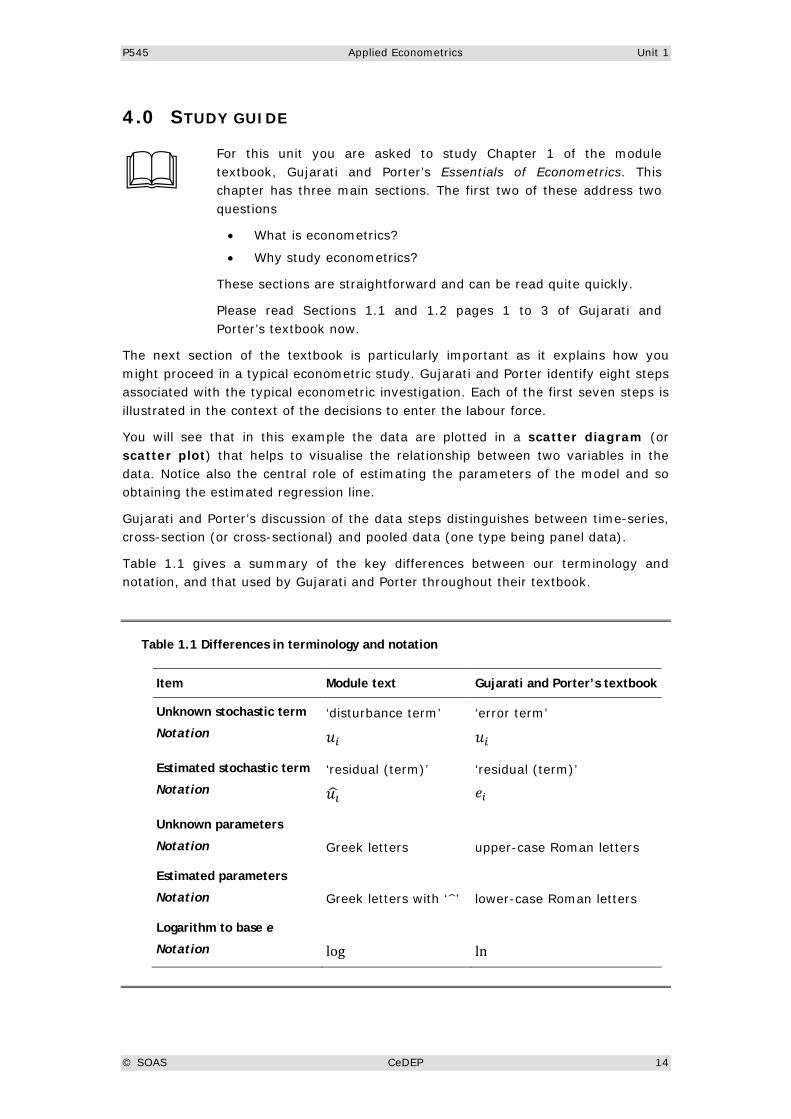
Table 1.1 gives a summary of the key differences between our terminology and notation, and that used by Gujarati and Porter throughout their textbook.

Table 1.1 Differences in terminology and notation

Item Module text Gujarati and Porter’s textbook

Unknown stochastic term

Notation

‘disturbance term’

𝑢𝑖 ‘error term’

𝑢𝑖

Estimated stochastic term

Notation

‘residual (term)’

𝑢𝚤�

‘residual (term)’

𝑒𝑖

Unknown parameters

Notation

Greek letters

upper-case Roman letters

Estimated parameters

Notation

Greek letters with ‘ �’

lower-case Roman letters

Logarithm to base e

Notation

log

ln


© SOAS CeDEP 15

Although these differences are inconvenient, it is an unfortunate fact that terminology and notation are not wholly standardised amongst econometricians and such discrepancies are often encountered.

Now please carefully read Section 1.3, pages 3 to 13 of the textbook.


© SOAS CeDEP 16

5.0 AN EXAMPLE: THE KEYNESIAN CONSUMPTION FUNCTION

The eight steps explained in the textbook are typical of any econometric investigation. We shall now illustrate seven of them with another example, the Keynesian consumption function.

Statement of the theory

The Keynesian theory of consumption is the basis of our model of consumption expenditure. This theory states that real consumption expenditure depends on real disposable income, other things held constant. (Keynes also identified many other factors that potentially affect consumption expenditure − whether or not they do is of course an empirical question − and he divided them into ‘objective’ and ‘subjective’, which he discusses in Chapters 8 and 9 respectively of his General Theory of Employment, Interest and Money.) When income rises, consumption expenditure rises, but changes in consumption expenditure are less than the change in income. Also, as income rises, the average propensity to consume, that is, consumption per unit of income, falls.

Mathematical model of the theory

Suppose we represent the Keynesian consumption function as a linear relationship

𝑌 = 𝛽1 + 𝛽2𝑋 (1.10)

where 𝑌 is real consumption expenditure, 𝑋 is real disposable income, 𝛽1 is a

constant and 𝛽2 is the slope of the consumption function, that is, the marginal

propensity to consume out of disposable income. Because of our a priori expectations concerning the average and marginal propensities to consume, we expect 𝛽1 > 0 and

0 < 𝛽2 < 1. (Note that the average propensity to consume is 𝑌 𝑋⁄ = (𝛽1� 𝑋)⁄ + 𝛽2. For this to fall as income rises, we need 𝛽1 > 0.)

Econometric model of the theory

The econometric model is stochastic. It includes a random disturbance, u, which captures the influence of all the other variables that may influence consumption expenditure.

𝑌 = 𝛽1 + 𝛽2𝑋 + 𝑢 (1.11)

Collection of data

The data to be used are annual time-series data for the UK covering the period 1955−1991. They are aggregate consumption expenditure and personal disposable income both measured in £(1985) million. The source of the data is the Economic Trends Annual Supplement 1991. Thus, our model represents a theory about the


© SOAS CeDEP 17

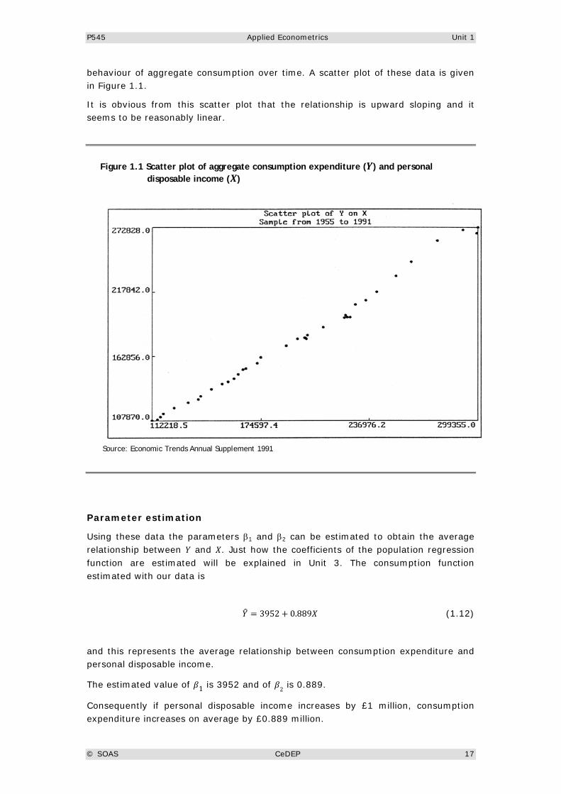
behaviour of aggregate consumption over time. A scatter plot of these data is given in Figure 1.1.

It is obvious from this scatter plot that the relationship is upward sloping and it seems to be reasonably linear.

Figure 1.1 Scatter plot of aggregate consumption expenditure (𝒀) and personal disposable income (𝑿)

Source: Economic Trends Annual Supplement 1991

Parameter estimation

Using these data the parameters β1 and β2 can be estimated to obtain the average relationship between 𝑌 and 𝑋. Just how the coefficients of the population regression function are estimated will be explained in Unit 3. The consumption function estimated with our data is

𝑌� = 3952 + 0.889𝑋 (1.12)

and this represents the average relationship between consumption expenditure and personal disposable income.

The estimated value of 𝛽1 is 3952 and of 𝛽2 is 0.889.

Consequently if personal disposable income increases by £1 million, consumption expenditure increases on average by £0.889 million.


© SOAS CeDEP 18

The interpretation of the intercept is not so meaningful. Mechanical interpretation of the estimate tells us that consumption expenditure is £3952 million if aggregate personal disposable income is zero. However, this is not particularly helpful because if aggregate personal disposable income is zero then the economy would be in chaos and the Keynesian theory of consumption expenditure would not be appropriate. The fact is that, in our sample, the 𝑋-values are a long way from zero, and we really have no idea what the consumption function might look like at low levels of income.

Tests of the hypothesims

Do the results conform to the theory of the consumption function?

With our theory we expect 𝛽1 > 0 and 0 < 𝛽2 < 1.

Is each of these hypotheses supported by the results? Clearly, our estimates are consistent with what we expected to obtain, but we must wait until Unit 4 for a discussion of formal hypothesis tests.

Prediction

We can use the estimated model to predict what consumption expenditure would be if personal disposable income were a particular amount. Suppose personal disposable income was £250 000 million. The predicted amount of consumption expenditure is

𝑌� = 3952 + 0.889(250 000)

∴ 𝑌� =226 202

That is, consumption expenditure is predicted to be £226 202 million if disposable income is £250 000 million.


© SOAS CeDEP 19

SELF ASSESSMENT QUESTIONS

uestion 1.1

What are the links between econometrics and both economic theory and mathematical economics?

For the rest of the questions, you will need to use R software. Please turn to the R Guide for Unit 1 now and follow the instructions given.

uestion 1.2

The data file u1q2.txt contains annual time-series data for the United States over the period 1959−1991 on aggregate consumption expenditure, 𝐶, and disposable income, 𝑌, both measured per head of population and in billions of constant 1987$. The source of the data is Economic Report of the President, 1992, table B-5, page 305.

• Use R software to produce a scatter plot of 𝐶 on the vertical axis and 𝑌 on the horizontal axis. Comment on the scatter plot: would a linear regression seem appropriate?

• Use R software to obtain time-series plots of 𝐶 and 𝑌. Describe the way consumption and income have moved over the period 1958−1991.

uestion 1.3

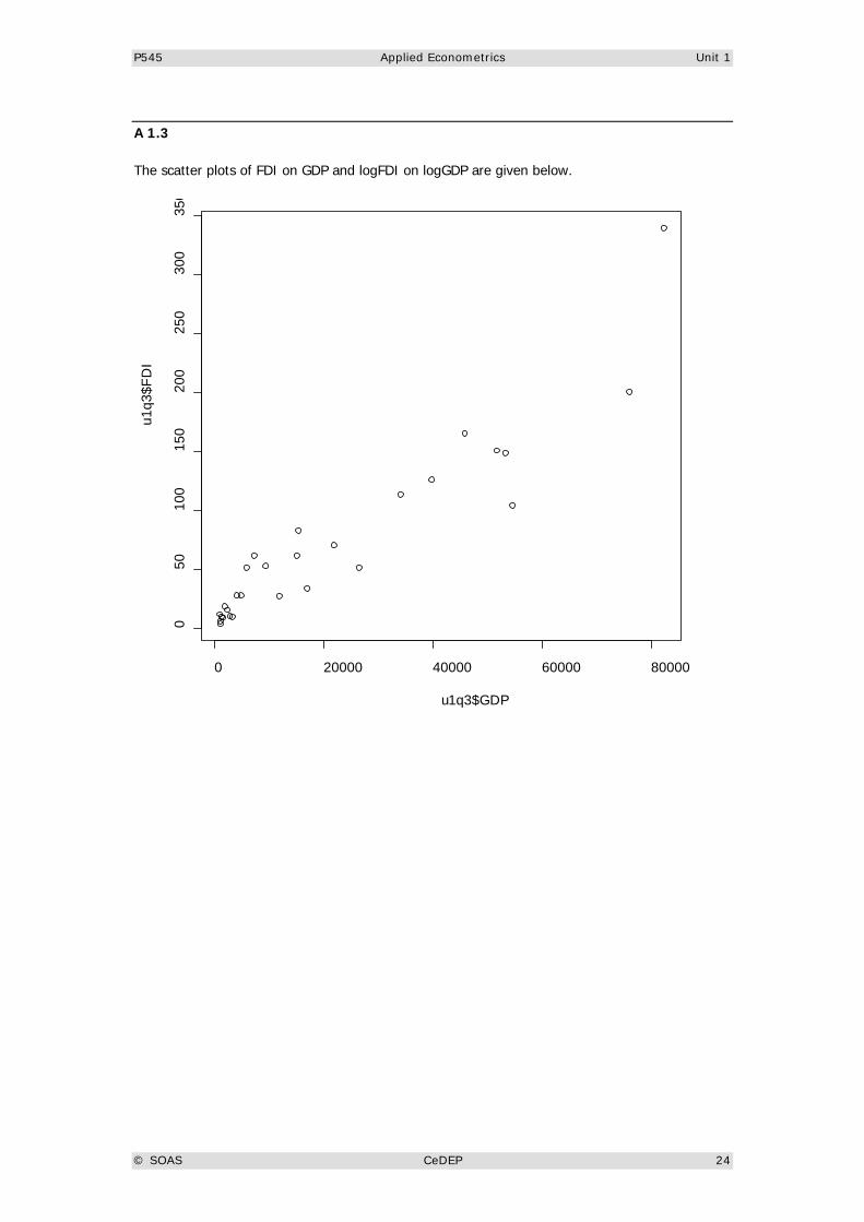
The hypothesis that foreign direct investment is determined by demand suggests that foreign direct investment and gross domestic product are positively related, other variables remaining constant. The data file u1q3.txt contains annual time-series data for the period 1958−1985 on foreign direct investment, FDI, and gross domestic product, GDP, for Taiwan. The source of these data is Pan-Long Tsai, ‘Determinants of foreign direct investment in Taiwan: an alternative approach with time series data’, World Development, 1991, Table A-1, page 285.

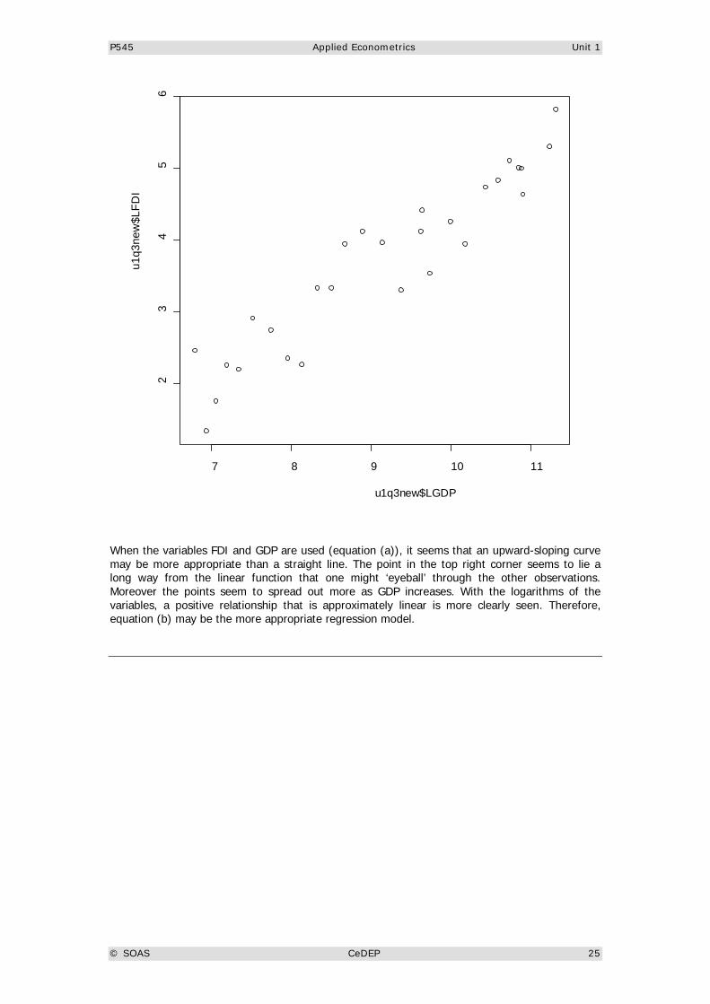
Use R software to obtain scatter plots of FDI on GDP and the logarithm of FDI on the logarithm of GDP, both for the period 1958−1985. Comment on the two scatter plots. Which of the following would you expect to be the more appropriate linear regression model:

(a) 𝐹𝐷𝐼 = 𝛽1 + 𝛽2𝐺𝐷𝑃+ 𝑢 ? or

(b) logFDI = 𝛾1 + 𝛾2log𝐺𝐷𝑃 + 𝑣 ?

Q

Q

Q


© SOAS CeDEP 20

uestion 1.4

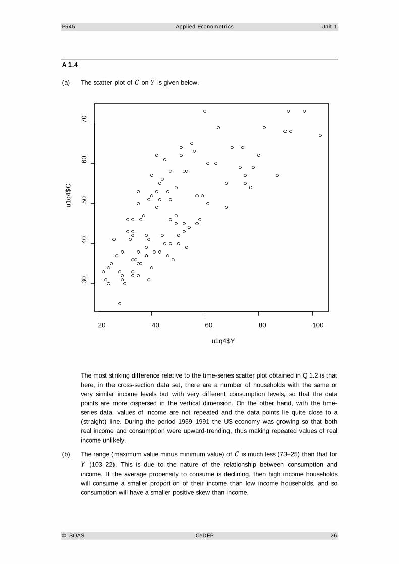
The data file u1q4.txt contains cross-section data from a sample of 100 rural households on the value of their consumption and income during a given month. Income (𝑌) includes cash income from all sources during the month concerned, plus the (imputed) market value of own production consumed by the household. Consumption (𝐶) includes the value of all purchased items, plus the value of own production consumed by the household. The units are measured in the local currency rounded to the nearest whole number.

(a) Obtain the scatter plot of 𝐶 on 𝑌. What is the main difference between this scatter plot and the one constructed in Q 1.2?

(b) Use R software to obtain the histograms of 𝐶 and 𝑌. Income has the usual positively skewed distribution that we would expect, whereas the distribution of consumption is less skewed. Can you suggest a reason for this?

(c) Use R software

(i) to obtain the average propensity to consume at the sample means

(ii) to compare the degree of skewness of the two variables

(iii) to obtain their correlation coefficient.

uestion 1.5

Weekly earnings can vary considerably in the case of casual dock labourers recruited on a day-to-day basis. There are differences between workers as well as across weeks. Weekly earnings will vary from week to week depending on the activity of the harbour which determines the demand for labour. Daily recruitment will be high if demand is high, and vice versa. Earnings also vary between workers in any given week. These depend on the numbers of days a worker manages to get recruited for in a particular week, on whether he or she is recruited for the day shift or the night shift, and on the number of hours of overtime he or she works in that week.

In this exercise you will look at data on the weekly earnings of casual workers, ECAS, and the recruitment of casual workers, CASREC. The data file u1q5.txt contains paired observations on the two variables ECAS and CASREC. The data were taken from a field study carried out in 1980/81 by the Centre of African Studies in Mozambique (Eduardo Mondlane University, Maputo) on casual labour on the docks of Maputo harbour. The earnings data are in units of 100 MT, the local currency being the Metical.

(a) Using R software, calculate the means, standard deviations, and minimum and maximum values for both variables.

(b) A particular worker is randomly chosen from the labour force in a particular week in 1980/1981 that is also randomly chosen. Using the information in your answer to part (a), what is your best estimate of the weekly earnings of this randomly selected worker?

(c) With R software, obtain the scatter plot of ECAS against CASREC. Write down what you observe.

Q

Q


© SOAS CeDEP 21

UNIT SUMMARY

In this unit we have introduced some basic ideas on econometrics and regression analysis. The most important points to remember are the following.

• Econometrics is the application of statistical and mathematical methods to the analysis of economic data, with the purpose of giving empirical content to economic theories and testing them against ‘reality’.

• The econometrician’s approach differs from that of the economic theorist because

- we cannot ‘hold other things constant’ in empirical analysis

- the random nature of relationships between variables means that the results and conclusions of empirical analysis always contain an element of uncertainty

- there is a discrepancy between theoretical variables and observed data in terms of coverage and precision of measurement

- econometricians cannot avoid explicit assumptions about the time frame of their model, since the data they use have been generated in a ‘real-time’ context

• Regression analysis is the statistical basis of econometric theory and practice. Its aim is to quantify relationships between variables, especially between variables whose relationship is subject to chance variation.

• Regression involves finding an average line that summarises the relationship whereby 𝑌 depends on 𝑋 in the midst of random variation and uncertainty of outcome.

• The randomness inherent in conclusions and outcomes based on regression analysis is formally modelled by introducing a disturbance term into our behavioural equations. This is a stochastic variable which is not observable. However, the residuals of a sample regression function may provide us with an indication as to the behaviour of these unknown disturbances.

• Regression allows us to investigate the association between variables, but it cannot ‘discover’ causality between them. To establish causality we need to resort to economic theory.

• Empirical work in economics cannot rely on experimentation. Econometric analysis is therefore based on careful observation of data drawn from within a context which we do not control.

In terms of practical skills, this unit requires that

• you are familiar with the scatter plot as a practical tool of empirical analysis

• you know how to load data into R software from a pre-existing data file

• you know the R software commands to obtain a summary of descriptive statistics of a variable, make a scatter plot and create logarithms of variables


© SOAS CeDEP 23

ANSWERS TO SELF ASSESSMENT QUESTIONS A 1.1 Economic theory can be viewed as a set of qualitative relationships between variables. Such theory can frequently be written in the form of a mathematical model. An econometric model may be obtained from an appropriate mathematical model with the addition of a random error term. By using data to estimate the econometric model we can in effect quantify economic relationships.

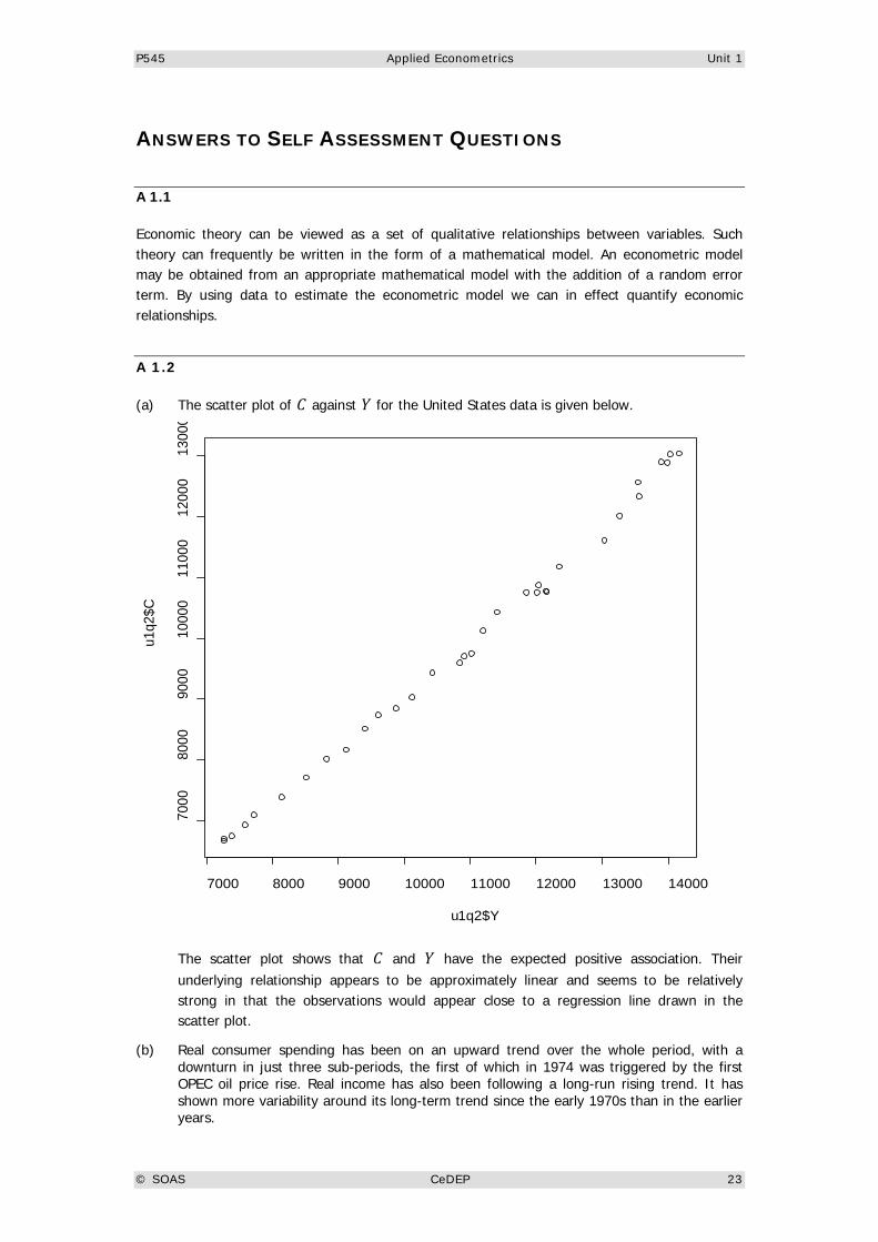
A 1.2 (a) The scatter plot of 𝐶 against 𝑌 for the United States data is given below.

The scatter plot shows that 𝐶 and 𝑌 have the expected positive association. Their underlying relationship appears to be approximately linear and seems to be relatively strong in that the observations would appear close to a regression line drawn in the scatter plot.

(b) Real consumer spending has been on an upward trend over the whole period, with a downturn in just three sub-periods, the first of which in 1974 was triggered by the first OPEC oil price rise. Real income has also been following a long-run rising trend. It has shown more variability around its long-term trend since the early 1970s than in the earlier years.

7000 8000 9000 10000 11000 12000 13000 14000

7000

8000

9000

1000

011

000

1200

013

000

u1q2$Y

u1q2

$C


© SOAS CeDEP 24

A 1.3

The scatter plots of FDI on GDP and logFDI on logGDP are given below.

0 20000 40000 60000 80000

050

100

150

200

250

300

350

u1q3$GDP

u1q3

$FD

I


© SOAS CeDEP 25

When the variables FDI and GDP are used (equation (a)), it seems that an upward-sloping curve may be more appropriate than a straight line. The point in the top right corner seems to lie a long way from the linear function that one might ‘eyeball’ through the other observations. Moreover the points seem to spread out more as GDP increases. With the logarithms of the variables, a positive relationship that is approximately linear is more clearly seen. Therefore, equation (b) may be the more appropriate regression model.

7 8 9 10 11

23

45

6

u1q3new$LGDP

u1q3

new

$LFD

I


© SOAS CeDEP 26

A 1.4

(a) The scatter plot of 𝐶 on 𝑌 is given below.

The most striking difference relative to the time-series scatter plot obtained in Q 1.2 is that here, in the cross-section data set, there are a number of households with the same or very similar income levels but with very different consumption levels, so that the data points are more dispersed in the vertical dimension. On the other hand, with the time-series data, values of income are not repeated and the data points lie quite close to a (straight) line. During the period 1959−1991 the US economy was growing so that both real income and consumption were upward-trending, thus making repeated values of real income unlikely.

(b) The range (maximum value minus minimum value) of 𝐶 is much less (73−25) than that for 𝑌 (103−22). This is due to the nature of the relationship between consumption and income. If the average propensity to consume is declining, then high income households will consume a smaller proportion of their income than low income households, and so consumption will have a smaller positive skew than income.

20 40 60 80 100

3040

5060

70

u1q4$Y

u1q4

$C


© SOAS CeDEP 27

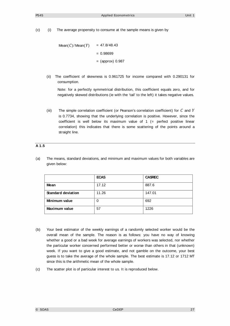
(c) (i) The average propensity to consume at the sample means is given by

Mean(𝐶)/Mean(𝑌) = 47.8/48.43

= 0.98699

= (approx) 0.987

(ii) The coefficient of skewness is 0.961725 for income compared with 0.290131 for consumption.

Note: for a perfectly symmetrical distribution, this coefficient equals zero, and for negatively skewed distributions (ie with the ‘tail’ to the left) it takes negative values.

(iii) The simple correlation coefficient (or Pearson’s correlation coefficient) for 𝐶 and 𝑌 is 0.7734, showing that the underlying correlation is positive. However, since the coefficient is well below its maximum value of 1 (= perfect positive linear correlation) this indicates that there is some scattering of the points around a straight line.

A 1.5

(a) The means, standard deviations, and minimum and maximum values for both variables are

given below:

ECAS CASREC

Mean 17.12 887.6

Standard deviation 11.26 147.01

Minimum value 0 692

Maximum value 57 1226

(b) Your best estimator of the weekly earnings of a randomly selected worker would be the overall mean of the sample. The reason is as follows: you have no way of knowing whether a good or a bad week for average earnings of workers was selected, nor whether the particular worker concerned performed better or worse than others in that (unknown) week. If you want to give a good estimate, and not gamble on the outcome, your best guess is to take the average of the whole sample. The best estimate is 17.12 or 1712 MT since this is the arithmetic mean of the whole sample.

(c) The scatter plot is of particular interest to us. It is reproduced below.


© SOAS CeDEP 28

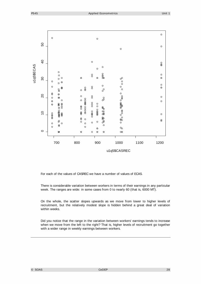
For each of the values of CASREC we have a number of values of ECAS.

There is considerable variation between workers in terms of their earnings in any particular week. The ranges are wide: in some cases from 0 to nearly 60 (that is, 6000 MT).

On the whole, the scatter slopes upwards as we move from lower to higher levels of recruitment, but the relatively modest slope is hidden behind a great deal of variation within weeks.

Did you notice that the range in the variation between workers’ earnings tends to increase when we move from the left to the right? That is, higher levels of recruitment go together with a wider range in weekly earnings between workers.

700 800 900 1000 1100 1200

010

2030

4050

u1q5$CASREC

u1q5

$EC

AS

centre for development, environment and policy p545 ... normal linear regression model. • to show...

Documents