regression models - home | princeton universitydeaton/downloads/testing_linear_versus...regression...
TRANSCRIPT
Review of Economic Studies (1980) XLVII, 275-291 0034-6527/80/00130275$02.00 (g? The Society for Economic Analysis Limited
Testing Linear versus Logarithmic
Regression Models GWYN ANEURYN-EVANS
University of Cambridge
and
ANGUS DEATON University of Bristol
INTRODUCTION
One of the problems most frequently encountered by the applied econometrician is the choice between logarithmic and linear regression models. Economic theory is rarely of great help although there are cases where one or other specification is clearly inap- propriate; for example, in demand analysis constant elasticity specifications are inconsis- tent with the budget constraint. Nor are standard statistical tests very useful; R2 statistics are not commensurable between models with dependent variables in levels and in logarithms and the comparison of likelihoods has no firm basis in statistical inference. In this paper, we develop a practical text based upon Cox's ((1961) and (1962)) procedure for testing separate families of hypotheses; the work is thus an extension of earlier econometric applications of Cox's test to single equation linear regressions in Pesaran (1974) and to many equation non-linear regression in Pesaran and Deaton (1978). The test we develop here is applicable to two competing single-equation models, one of which explains the level of a variable up to an additive error, the other of which explains its logarithm, again up to an additive error. Hence, in terms of the levels of the variables, we are testing for multiplicative versus additive errors, and it is this which differentiates this paper from the earlier work in which an additive error was always assumed. We shall also allow, as in the earlier papers, the deterministic parts of the regressions to be linear or non-linear and to have the same or different independent variables; it is thus possible to test for functional form and specification in a very general way.
Section 1 of the paper defines the problem and derives the test statistics. The formulae allow the calculation of two statistics, No and N1 say, the first of which is asymptotically distributed as N(0, 1) if the logarithmic specification is correct, the second, for all practical purposes, as N(0, 1) if the linear model is true. Section 2 discusses problems associated with the calculation of the statistics and shows how they can be surmounted. Section 3 presents the results of Monte-Carlo experiments designed to evaluate the potential of the test in practice. We investigate, in particular, the shape of the actual distributions of No and N1 in samples of sizes 20, 40 and 80 as well as comparing the performance of the Cox procedure with that of the likelihood ratio test, as proposed by Sargan (1964). Finally, we offer some evidence of the ability of the procedure to detect total misspecification when neither of the hypotheses is true. Section 4 contains a summary and conclusions.
The general issues of statistical inference raised by the use of the Cox procedure in econometrics as well as alternative testing procedures have already been widely discussed, see Pesaran and Deaton (1978), Quandt (1974) and Amemiya (1976). In this case, however, there exists one very obvious alternative procedure. This is to specify the model,
275
276 REVIEW OF ECONOMIC STUDIES
not in levels or in logarithms, but via the Box-Cox transform; hence, the dependent variable is (ya - 1)/a, so that with a = 1, the regression is linear, with a = 0, it is logarithmic, these cases being only two possibilities out of an infinite range as a varies. The general model can be estimated by grid search or by non-linear maximization of the likelihood and a maximum likelihood estimate for a obtained. The values of 0 and 1 can then be compared using a conventional likelihood ratio test. A number of comments may be made. Note that the problem is now rather different from the one originally posed. We no longer have a discrete choice between a = 0 and a = 1 but instead have to choose between one or both of these and the maximum-likelihood estimate, a', say. One possible difficulty is that the investigator may only be interested in linear or logarithmic forms so that a value for ca of 0 73, for example, may not be very useful. It is our impression that many econometricians would simply adopt a rule which chooses the linear form when or > 0 5 and the log-linear a <0 5. If so, a straightforward comparison of likelihoods between the two cases is much more appropriate, and, in Section 3, we shall examine the performance of such a rule. However, it may well be that the investigator has no prior preference for either the logarithmic or linear forms so that any value for cx is perfectly acceptable. In this case, the correct procedure is to estimate the Box-Cox model and use the value of ca which emerges; no problem of choice or of inference arises. The final possibility is that the true model may not be included even in the general form. In this case, estimation of a and comparison with 0 and 1 will be of no help; the whole experiment is being conducted within a false maintained hypothesis and is meaningless. The Cox procedure, however, encompasses the possibility of rejecting both models which is, in this case, the only correct decision. Whether in fact it will do so is a matter for empirical investigation and we shall return to the question in Section 3.
1. THE DERIVATION OF THE TEST STATISTICS
1.1. Specification of the Models
There are two models to be compared, Ho and H1. These are defined by
Ho: ln yt = ft(x, 8o) + Eot*,
Hi: yt= gt (z, 01) + E i t, ...(2)
where Yt is the tth observation on the dependent variable, t = 1, ..., T; 6o and 01 are ko and k1 vectors of parameters, and x and z are vectors of independent variables. There is no restriction on the variables which appear in x and z; they may be the same, different or transformations of one another. The functions ft and gt may or may not be linear. For Cot, we assume
Eot - N(O, _2 ). ... (3)
It is not, however possible to assume Et- N(0, o2) since, if this were so, there would always be a finite probability of Yt becoming non-positive. If so, Ho must be false since the logarithm does not exist, and the problem of inference is a trivial one. Consequently, if it is possible to give serious consideration to Ho, the distribution of Elt must be such as to ensure that y is positive. Various distributions could be used which would meet this criterion. For example, we could follow Amemiya (1973) and truncate Elt so that Yt is given by (2) if the right hand side is greater than some positive number, a, say, and equal to a otherwise. Alternatively and in some respects more simply, we can truncate the distribution of elt at a fixed number of standard deviations from zero. Here we use the normal distribution and it is convenient to truncate symmetrically, i.e. if fN(x; 0.2) is the p.d.f. of an N(0, a2) variable and if r(Eit) is the p.d.f. of Elt, we write
Tr(Elt) = a>o (k)fN((at; )1 ) ?tl < kor
= 0 | ?1tl > ka, ... (4a)
ANEURYN-EVANS & DEATON LINEAR VERSUS LOGARITHMIC 277
where
a(k) = (27)-e t2/2dt} ...(4b)
The fact that Ho is to be seriously considered will be taken to imply that k can be set a priori at some large value (k ? 6 say). For values of k of the size indicated a is so close to unity that, for many purposes, we can assume E1t -N(O, 1o). If, on the other hand, we are not prepared to assert that gt(z, 01) is always at least 6 to 8 equation standard errors above zero, then it is not sensible to regard both Ho and H1 as possible.
Let us write a0 and ai for the extended parameter vectors of the two models, so that = (6I, a2 ) and a' = (61, U2 ). Denote the log likelihood functions of Ho and H1 by
Lo(ao) and Ll(al) respectively and by Llo the log of the maximum likelihood ratio. Then, if Ho is true, we must calculate
To = L1o - T{ plimo (L) } a(5)
where plimo denotes the probability limit when Ho is true and denotes a maximum likelihood estimate. If Lio = Lo(ao) -Ll(alo), where aio = plimo a',, then Cox (1962) has shown that, if Ho is true, To is asymptotically normally distributed with mean zero and variance V0(T0), given by
1 t - Vo( To) = Vo(L lo)-T- 71 1 (6)
T
where Q is the asymptotic information matrix of Ho,
Q = -plimo - ..L (7) T caaoaa'o
and
a [plimo (L1o/ T)] * (8)
If H1 is true, similar expressions yield T1 and V1(T1).
The two log likelihood functions are given by
T T 2 2~O Lo(ao)= --ln(2ir)--Inuo- 2 I-nyt . (9) 2 2 2r
and
T T 2Zi Ll(a) =--Iln (2Xr)--Iln a- 2t+ T In a(k) ... (10)
2 2 2o
where the extra sum in (9) is the log of the product of the Jacobians. Maximum likelihood estimates 6o, co, i, a1 satisfy
(JO = E{ln Yt -nfty(0f
Y. ,a {ln yt - ft (00)} = 0, j= ... ko ...(12)
2=1 t{Yt_gt(0 ... (13)
278 REVIEW OF ECONOMIC STUDIES
Y.tag(l ly {Y- t(0^l1)= , j=L1 ...,~ ki ... (14) a lj
where, for convenience, the x and z arguments of f and g have been suppressed. The maximized log likelihood ratio L1o is thus
Ll= -n (-A) -ZtIn yt -Tlna(k). . .. (15) 2 (TO ***(
Note that L1o is itself a possible candidate for discriminating between Ho and H1 as has been suggested by Sargan (1964). The models are, of course, not nested, so that we do not have the usual justification for the statistic. Nevertheless, it is simple to calculate and, to the extent that likelihoods can be regarded as fundamental measures of plausibility, see in particular Edwards (1972), Llo is a natural quantity to inspect.
1.2. Calculation of To
Having laid this groundwork, we begin with the easier case, when Ho is true. Writing a 1o for plimo a^, so that a 10 is plimo 15, from (15) and (1)
2
TI 1 =-0n lT - -n al( -kt(0o). ...a(16)
Hence, writing (Tl for the ML estimate of U20 To is given by
T A2
2 1o
Note that in many applications, for example when ft is linear, the sum on the right hand side of (17) will be zero. The maximum likelihood estimate 1l, and hence clo, can be calculated by solving
Eo(L(c) 0. . .. (18) aa 10
But
L1(a 1o) = --In (2) T--l no - 2 Zt {Yt - gt(10)}2 + T ln a (k) . .. (19) 2 2 1o
Hence
IaLl(alo)\ T 1 y Eo ao-20 = - 220 + 2-4EoE.t{yt-gt(01o)}2. ... (20)
This can be further evaluated by writing yt = eft(0o)+?ot. In this and the sequel, the following expectations are useful
Eo(y') - erft(0o)er2c/2 . .. (21 a)
Eo(oty) - ru2 e rf(0)er eJo/21 . . . (2 1b) Eo(8 otY r) 2 r 4 rf'(06)e r2o-2/2 + (oe rf'(06)e r2o-2/2 ... (2 ic)
Hence
Eo[Z {Y t2 - 2gt(6lo)yt + gt(o10) 2}]
=. t { Yote? - 2gt(6lo)yot+gt(61o)2}
= Zt {Yot - gt (10)}2 +E yt(eY -1), ...(22)
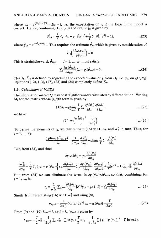
ANEURYN-EVANS & DEATON LINEAR VERSUS LOGARITHMIC 279
where yot =-e 0 EO(y), i.e. the expectation of Yt if the logarithmic model is correct. Hence, combining (18), (20) and (22), ao- is given by
A0 T t I Yot _gt ( "10)12 + A
Et Y t; ...2 3 ioT T to
where pot = eft(6o) 0 /2. This requires the estimate O10 which is given by consideration of
E LO(alod1)) 0 Eo 0.o
This is straightforward; 0101, j = 1, ..., k1 must satisfy
Et _ Yot - gt00)} = 0. . . . (24)
Clearly, 010 is defined by regressing the expected value of y from Ho, i.e. yo, on g(z, 01). Equations (12), (13), (17), (23) and (24) completely define To.
1.3. Calculation of Vo(To)
The information matrix Q may be straightforwardly calculated by differentiation. Writing Mf for the matrix whose (i, j)th term is given by
(Mf)zi=plimo 1
Etaft(00)at(800) ... (25) T--oo T aoi 80i
we have
o-1 = ( f
4 ... (26)
To derive the elements of -q, we differentiate (16) w.r.t. 00j and o-o in turn. Thus, for j= 1, ..., ko
2 a plimo (Llo/T) 1 acr0 l 1 aft(00)
-2o ~ 00-plimo--Et a00j
aoao T a0
But, from (23), and since
ayot/800o = Yot aft(0o)
0 2 af ft(0o) agt(010) a0lOk 2 _2a2 ft(0o)
=-i EtlY0t-gt(010)1 Yot a00 k-L
*OO ao +Te ?- t E t o0 8doj YT 800j - 800k 80101 I 800j
But, from (24) we can eliminate the terms in agt(100)/8O1k, so that, combining, for j=1, ...,ko
1 aft(0o) f2 at(0o) 7i = 2 Et Yot eY0t gt(010)- . . .(27)
10o a80O 80Oo
Similarly, differentiating (16) w.r.t. 0 and using (8),
1 r o~2eyo lY T 7lko+1 = 2 Et yoto2eyot- gt(010)1 - 2... (28)
2C10 2aO2
From (9) and (19) L1o = Lo(ao)-L1(a lo) is given by
T 2 1 2 T 2 1 EIy t( 01 Lio=--(uo- 2 EtEot -lnyt+-Iy o+ 2 {yt-gt(01o)}2-Tlna(k). 2 20o 2 2lo
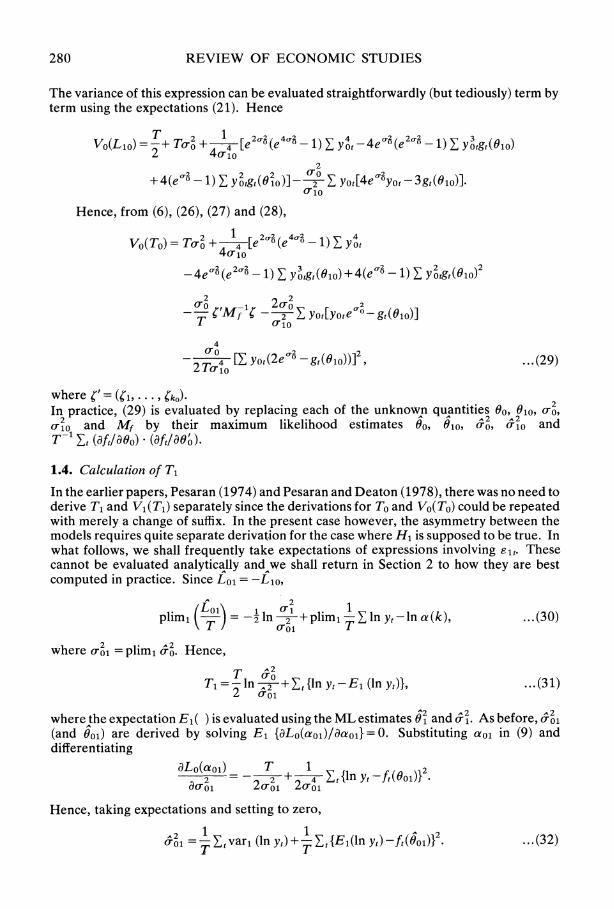
280 REVIEW OF ECONOMIC STUDIES
The variance of this expression can be evaluated straightforwardly (but tediously) term by term using the expectations (21). Hence
Vo(L1o) + T+ o + 14 [e r(e E -4e02(e E 3 2 4o10
2
+ 4(eCQ - 0) E Y20tgt( 210 - 2 E Yot[4eo'gyot - 3gt(0lo)]. 10io
Hence, from (6), (26), (27) and (28),
- 2 e2a> _1) E y3tgt(0lo) +4(e -1) y2tgt(01?)2
22
- C f M _ o Y. y0t[y0oteO-gt(O1o)]
4 CO
4[yot(2e'g -gt(10l))]2 -*29 2ToK ...(29) 2Tolo
where 'k ) .. ., .k0)
In practice, (29) is evaluated by replacing each of the unknown quantities GO, 910, 20, 2lo and Mf by their maximum likelihood estimates do, 910 2 co, A2i and
T 1 Et (dft/dSo) * (dftdaoo).
1.4. Calculation of T1
In the earlier papers, Pesaran (1974) and Pesaran and Deaton (1978), there was no need to derive T1 and V1(T1) separately since the derivations for To and Vo(To) could be repeated with merely a change of suffix. In the present case however, the asymmetry between the models requires quite separate derivation for the case where H1 is supposed to be true. In what follows, we shall frequently take expectations of expressions involving Elt. These cannot be evaluated analytically and we shall return in Section 2 to how they are best computed in practice. Since Lo1 =-Lio
2
plim1 =-ln +2 +plimn -ZE (ln yIn a(k), ... (30)
2 2o
where the expectation E1( ) is evaluated using the ML estimates 01 and 1. As before, U' oi (and 001) are derived by solving E1 {aLo(aol)/aaoo1} =0. Substituting ao, in (9) and differentiating
aLo(aoi) T + 1 Et{ln yt-t (0?1)12.
dcr1 2(Tol f0
Hence, taking expectations and setting to zero,
O'oi =T var (InYt)+TEt El(lnyt)-ft(001)}2. ... (32)
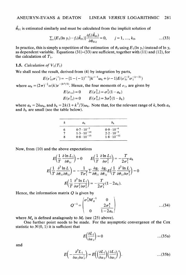
ANEURYN-EVANS & DEATON LINEAR VERSUS LOGARITHMIC 281
6o, is estimated similarly and must be calculated from the implicit solution of
E {Ei(ln y)-ft()at(1) = 0, j = 1, .. , ko- ...(33) ao;01 In practice, this is simply a repetition of the estimation of 0o using E1(ln Yt) instead of ln Yt as dependent variable. Equations (31)-(33) are sufficient, together with (11) and (12), for the calculation of T1.
1.5. Calculation of V (T1)
We shall need the result, derived from (4) by integration by parts,
( lt?1 ) {1-(-1)}kr 1zk+(r _l)E(r-2 -(r-2)) = - 1- (- 1)~'}lk' Ok + (r -1E(
where (Ck = (27r)-1a(k)e-(k /2). Hence, the four moments of ?lt are given by
E(Elt) = 0 E(e 2t) = o(1-ak)
E (E 3t) = O E (S 4t) = 3U41 (1 -bk)
where ak = 2kWk, and bk = 2k(1 + k2/3)Wk. Note that, for the relevant range of k, both ak
and bk are small (see the table below).
k ak bk
6 0 7 10-7 0.9 10-6
1-3 10 2-2 10 8 0.8.10-13 1.8. 10-12
Now, from (10) and the above expectations
Et1 a ln Ll 1( a? In L T E( aL1=0 E 2 Y ak
(T a d i Ttl) Tr2EaR a?Rl jE Tad_o) (1 a 2IntL 1 agd agT (1a )2InL
T aol1ao91 / *Tu1 ao1,i ae, 'T o1j-1 (1 a 2In L1\ T
E y2 24~(1-2ak).
Hence, the information matrix Q is given by
Q-1 =
~~~2cr4 ... (34) 0 1-2ak
where Mg is defined analagously to Mf (see (25) above). One further point needs to be made. For the asymptotic convergence of the Cox
statistic to N(0, 1) it is sufficient that
Et ) = 0 .(3 5a) aat
and
Et ala)=(a) ... (35b)
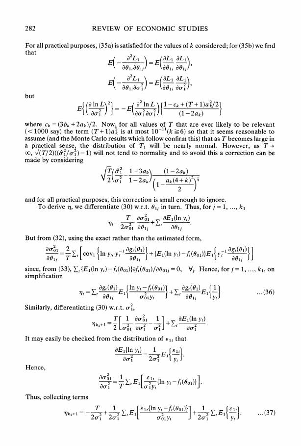
282 REVIEW OF ECONOMIC STUDIES
For all practical purposes, (35a) is satisfied for the values of k considered; for (35b) we find that 2
__a Li X Ll aLl aoljaoljJ kaol aolj
Etau 2Li ) (aLl aLl )
but f(alnL\21 aE IlnL l-ck+(T+l)ak/21 Et al) 1 E 12f (1-2ak) J
where Ck= (3bk+2ak)/2. Now, for all values of T that are ever likely to be relevant (<1000 say) the term (T+ 1)a2 is at most 10-11(k -6) so that it seems reasonable to assume (and the Monte Carlo results which follow confirm this) that as T becomes large in a practical sense, the distribution of T1 will be nearly normal. However, as T - Xo, /(T/2)((61/o2) - 1) will not tend to normality and to avoid this a correction can be made by considering
/T l 1-3ak\ (1 -2ak) U2
,- _ ) V 2 o1 l-2ak ak(4 2 )y
and for all practical purposes, this correction is small enough to ignore. To derive 71, we differentiate (30) w.r.t. Oij in turn. Thus, for j = 1, ...,
T aco1 aE1(ln yt) = 2 -o1 a
But from (32), using the exact rather than the estimated form,
801 2 r 1agt(tl)] f 1agt(oi)] t= T E covy {ln Yt, Yt g +{Ei(ln yt)-ft(0o1)}El Yt ag8oD]
since, from (33), EZ{El(ln Yt) -ft(001)}aft(0o1)/a0o1l = 0, V1. Hence, for j = 1, ..., kl, on simplification
Y. =tagt) (0In EInyt -ft(Ool)} ++ agjol) El 1 . ...(36)
Similarly, differentiating (30) w.r.t. ,
T7 1 2or 1 1 aEl(ln yt)
77kl+l= 2 2 ~
2 +Et 2 a[o1 aU27 ] I 2 0o 81 a- 1C
It may easily be checked from the distribution of E1t that
aE1{ln yt} 1 E Fit a2 2E- a1 2oi Yt
Hence,
Z2 =1tE1[ E {ln Yt- ft(Oo)}] 1 T U1Yt
Thus, collecting terms
T 1 2 2 E1t{ln Yt-ft(Ool)}] 1 Z Ei{ 1t} 71k, + =-j 2 +
2 EtEl 2+ 2 EtEl 1 ... (37) 2C1 21 (ToiYt 2 or1 Yt
ANEURYN-EVANS & DEATON LINEAR VERSUS LOGARITHMIC 283
Finally, from (10) and substitution of a01 in (9), Lo, =Li(a1)-Lo(aol) is given by
T O~i\ Z~t 1tY Lo, =-In (-2 )--2 +tln Yt+ 2 Yt{ln y-t(0ol)}2+ T In a((k). ...(38) 2 \oi 2o1 2coi
From this V1(Lo1) can be calculated term by term. Since very few of the relevant expectations can be simplified analytically, there is little point in deriving further algebraic expressions for this variance and the questions of computation will be taken up below. Once V1(Lo1) has been calculated, V1(T1) is calculated from, using (34),
22 4
Vi(Ti) = Vl(Lol) - g'Mg ; T T71k+l+ (1 - 2ak) . .. (39)
using (36) and (37) and replacing all unknown quantities by their ML estimates. (The quantity ak can be taken to be zero in practice.)
2. THE COMPUTATIONS OF THE TEST STATISTICS
The computation of To and Vo(To) poses no special difficulty. In general, both Ho and H1 will be estimated by non-linear techniques and the calculation of To requires one additional non-linear regression to estimate 010 and 5lo. The expression for Vo(To), (29), although complicated, is trivial enough to calculate. Unfortunately, this is not the case for T1 or V1(T1). For example, we require the expression E1(ln Yt) which is given by
r koI ln {gt(z, 01) + r} e ( 1 2
- kol v/2rui a for some suitable value of k, as well as a range of other expectations which arise in the calculation of V1(T1). Expressions like (40) can be evaluated each time they arise by numerical integration procedures but, in practice, this is prohibitively expensive even for practical work (e.g. if T = 60, there would be 600 or so integrations required for one test statistic), let alone for Monte Carlo experiments.
We therefore adopt the following alternative. Define v, a truncated N(0, 1) variable, by
v = 1/cr1 ... (41)
We can write r(v) for its density function so that (40) becomes
El(ln Yt) = J{ln gt(01) +ln (1 + 6v)}T(v)dv
= ln gt (01) + I ln (1 + ev) r (v)dv, . .. (42)
where l = ol/g,(01). On working through the expressions for T1 and its variance, all required expectations can be evaluated with the aid of integials of the form
k
I(a, b, c) = I 1 (+ V)a [In ( + eV)]bV ',7(v)dv, ... (43)
where e and v are as defined above and we require the ten integrals I(0, 1, 0), I(0, 2, 0), I (0, 3, 0), I (0, 4, 0), I (0, 1, 2), I (0, 2, 2,), I (- 1, 1,0), I (- 1, 1,1), I (- 1, 0,1), and I(-1, 0, 0). For given k, these integrals define ten functions of e, which we require for all values of e between zero and, say, 0 125. (If gt(61) > 8ol, it is not reasonable to consider Ho as a serious possibility.)
Each of the integrals was thus evaluated by numerical integration for values of 6 from 0 to 8 by intervals of 1/ 1024; the calculated values were then approximated by Chebycheff

284 REVIEW OF ECONOMIC STUDIES
polynomials. The polynomial coefficients were then built into the computer programme and used in routine evaluations of the statistics. This procedure worked extremely well. The calculations were very rapid compared with repeated quadrature and we were able to show that for reasonable values of k (6 to 10), the integrals were not sensitive to the precise value chosen. The programme was written so as to reject any value of e> 0 125; in this case, the Chebycheff approximations become unreliable but this is of no importance since, if this happens, Ho is clearly incorrect a priori.
3. SOME EMPIRICAL EVIDENCE
In this section, we present empirical evidence designed to elucidate the properties of the test, in particular, to investigate its distribution when either Ho or H1 is true and to discover how this is affected by sample size, and by other considerations. We also compare the Cox test with the unmodified likelihood ratio criterion suggested by Sargan (1964). Finally, we offer some tentative evidence for the case when neither Ho nor H1 is correct as specified. This last is perhaps the most important potential application of the test, but the possibilities are too vast to be more than touched on here.
Of particular interest for applications of the test is the question of how much guidance the large sample distributions of the statistics gives us about their behaviour in small or moderate-sized samples. The theory tells us that No= To/1 Vo is asymptotically dis- tributed as N(O, 1) under Ho and similarly for N1 under H1. However, we are ultimately interested in the joint distribution of No and N1 under both hypotheses and since both statistics are functions of the same magnitude, the log likelihood ratio, this can be done straightforwardly, at least asymptotically. To clarify, we change the notation slightly and write, from (5)
No= V(co) {L1o-Po(lao)} ... (44)
N1 = V(cIY2{-Llo+Pl(dl)} ... (45)
where Pa(cto)= T{plimo (Llo/T)}ao=o, Pa(c1)= T{plim1 (Llo/T)}1a=d,, we have used Lo= -Lo,, and the notation V0( ), V1( ), Po( ) and P1( ), emphasizes that the various magnitudes are evaluated as functions of the parameters of the current working hypothesis taken at their maximum likelihood values. For example, Vo is given by (29) as a function of ao and a10 but the latter is itself a function of a0 via (23) and (24) and, in practice, (29) and thus No is evaluated using the ML estimate of a0. If we rearrange (44) and (45), No and N1 satisfy (exactly),
No VO(c)2 + N1 V1 (c A1)2 = P1 (c A1) - Po(cto) . . . (46)
Hence, under Ho
[Vl(alo)] [, - _{P1(alo)-Po(ao)}] N(0, 1) (47)
while under H1
[Vo(ao) No], a1 - Po (aoto ]I
aNO ... (48)
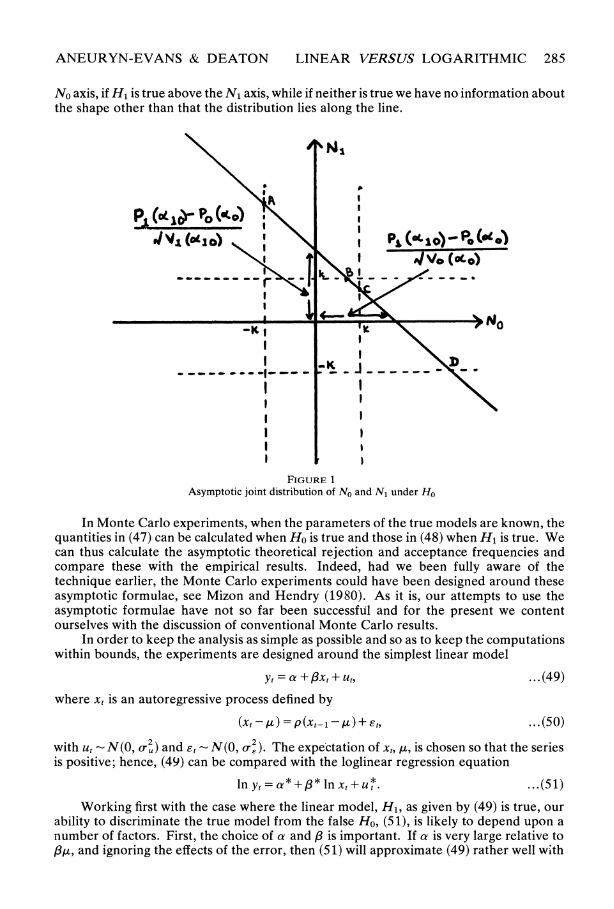
The situation when Ho is true is illustrated in Figure 1; as the sample becomes large No and N1 will lie along the line ABCD. A similar situation pertains when H1 is true although the line will have a different position and slope. In both cases ABCD moves away from the origin, maintaining its slope, as the sample size increases. The joint distribution of No and N1 is thus a singular one above the line ABCD. If Ho is true its mean lies always above the
ANEURYN-EVANS & DEATON LINEAR VERSUS LOGARITHMIC 285
No axis, if H1 is true above the N1 axis, while if neither is true we have no information about the shape other than that the distribution lies along the line.
V,(dO I PI I P=>l) -Po (at 0
-WK | l ly \NoP
.*K
JV __( ___1___ , _ _________
FIGURE 1 Asymptotic joint distribution of No and N1 under Ho
In Monte Carlo experiments, when the parameters of the true models are known, the quantities in (47) can be calculated when Ho is true and those in (48) when H1 is true. We can thus calculate the asymptotic theoretical rejection and acceptance frequencies and compare these with the empirical results. Indeed, had we been fully aware of the technique earlier, the Monte Carlo experiments could have been designed around these asymptotic formulae, see Mizon and Hendry (1980). As it is, our attempts to use the asymptotic formulae have not so far been successful and for the present we content ourselves with the discussion of conventional Monte Carlo results.
In order to keep the analysis as simple as possible and so as to keep the computations within bounds, the experiments are designed around the simplest linear model
Yt = a + fxt + ut, ...(49)
where xt is an autoregressive process defined by
(xt - A) = p (xt_-, ) + Et, ..(50)
with ut - N(O, o-b) and Et - N(O, o_ -). The expectation of xt, ,u, is chosen so that the series is positive; hence, (49) can be compared with the loglinear regression equation
ln Yt = a* +,I* ln xt + u . ...(51)
Working first with the case where the linear model, H1, as given by (49) is true, our ability to discriminate the true model from the false Ho, (51), is likely to depend upon a number of factors. First, the choice of a and ,B is important. If a is very large relative to ,I3,, and ignoring the effects of the error, then (51) will approximate (49) rather well with
286 REVIEW OF ECONOMIC STUDIES
a * = In a. Similarly, if a is close to zero, setting a * = ln 13 and 13* = 1 will make (51) close to (49). Consequently, values of a close to 13gt are likely to give us the best- chance of discrimination. The second important factor is the variance of xt; hence p and o-, are likely to be important. Finally, discrimination is likely to depend on o-r; when this is small, the linear model should fit so well as to rule out alternative specifications.
The experiments were carried out as follows. At a preliminary stage, six x, series, each of 80 observations, were generated corresponding to p = (0 5, 0 7, 0 9) and o-, =
(8, 16), using the normal random number generator G05ADF from the NAGLIB library. In each case, sufficient early values were discarded so as to ensure the arbitrary initial choice for x0 had negligible importance. The parameter , 2was set to 100 in all cases. All generated values of x, were positive. The parameter o- was controlled indirectly by setting the asymptotic R2 for the regression equation (49). Elementary manipulation leads to
plim R2= 13202/ (1 -p2) ...(52)
Given the extremely small probability of generating values of u, further than 8o-u from zero, no attempt was made to truncate the distribution. Given o- and p, oru can be chosen to set R2 at the desired level using (52). Three different sample sizes were used; for each replication, 80 observations of Yt were generated corresponding to x,. These were first used in a single test with sample size 80; each half of the sample (Yt and x,) was then used for two more tests of sample size 40. Finally, each half was itself subdivided to give four tests each with sample size 20. Each complete experiment was replicated 500 times. There are thus 500 replications for sample sizes 80, 1000 for sample sizes 40, and 2000 for sample size 20. The value of 13 was set to 5 throughout, with a at 500 (=,13A). Due to an oversight, it was not noticed that it is impossible to vary R2 for these values of a and 13 without creating a high probability of negative values of Yt. Thus, in the experiments where R2 is varied, a is set to 1000. The differences in results between a = 1000 and a = 500 were small enough to justify not repeating the earlier experiments.
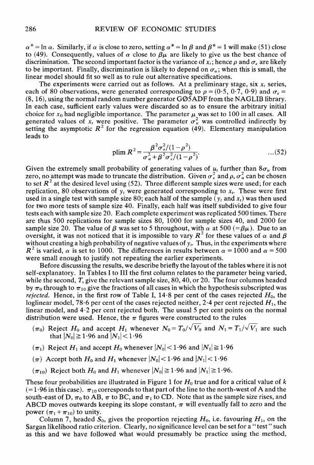
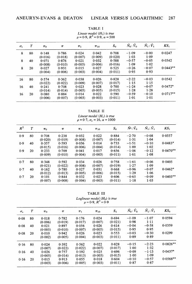
Before discussing the results, we describe briefly the layout of the tables where it is not self-explanatory. In Tables I to III the first column relates to the parameter being varied, while the second, T, give the relevant sample size, 80,40, or 20. The four columns headed by rro through to lri0 give the fractions of all cases in which the hypothesis subscripted was rejected. Hence, in the first row of Table I, 14X8 per cent of the cases rejected Ho, the loglinear model, 78-6 per cent of the cases rejected neither, 2-4 per cent rejected H1, the linear model, and 4X2 per cent rejected both. The usual 5 per cent points on the normal distribution were used. Hence, the Xr figures were constructed to the rules
(ITo) Reject Ho and accept H1 whenever NO = To/v4Vo and N1 = Ti/lV1 are such that INOI _ 1-96 and IN1I < 1-96
(IT1) Reject H1 and accept Ho whenever |NOl < 1X96 and |N11 _ 1X96
(IT) Accept both Ho and H1 whenever |NOl < 1X96 and 1N11 < 1X96
(X1r0) Reject both Ho and H1 whenever |NOl _ 1X96 and 1N11 - 1X96.
These four probabilities are illustrated in Figure 1 for Ho true and for a critical value of k (= 1X96 in this case). Ir0 corresponds to that part of the line to the north-west of A and the south-east of D, ITo to AB, IT to BC, and Ir1 to CD. Note that as the sample size rises, and ABCD moves outwards keeping its slope constant, IT will eventually fall to zero and the power (X1 + iro) to unity.
Column 7, headed S0, gives the proportion rejecting Ho, i.e. favouring H1, on the Sargan likelihood ratio criterion. Clearly, no significance level can be set for a " test " such as this and we have followed what would presumably be practice using the method,
ANEURYN-EVANS & DEATON LINEAR VERSUS LOGARITHMIC 287
TABLE I
Linear model (H1) is true p=0 9, R2= 9, a =500
oe T so i I Xo So N0:Vo N1:V1 KS1
8 80 0-148 0-786 0 024 0-042 0 708 -1-09 -0.00 0 0247 (0.016) (0.018) (0.007) (0-009) (0 020) 1 03 1-09
8 40 0 071 0 876 0 021 0 032 0 588 -0 57 -0 05 0 0342 (0-008) (0.010) (0 005) (0.006) (0.016) 1-09 1-02
8 20 0-027 0-931 0-015 0-027 0-525 -0-26 -0-07 0.0443** (0-004) (0-006) (0-003) (0.004) (0-011) 0*95 0-93
16 80 0-574 0 362 0 038 0-026 0*828 -2 22 -0-03 0-0542 (0.022) (0-022) (0.009) (0-007) (0-017) 1-15 1-15
16 40 0 241 0 708 0 023 0-028 0-700 -1 24 -0*07 0.0472* (0-014) (0-014) (0-005) (0-005) (0-015) 1-28 1-28
16 20 0-080 0-884 0-014 0-022 0-590 -0 59 -0-10 0.0717** (0 006) (0.007) (0-003) (0-003) (0-011) 1 01 1.01
TABLE II
Linear model (H1) is true p = 0-7, o = 16, a =1000
R2 T sIo IT I o So NgVo N1:V1 KS1
0 9 80 0-708 0-238 0 032 0-022 0-884 -2-70 -0-08 0-0557 (0-020) (0-019) (0 008) (0-007) (0-014) 1 31 1 04
0 9 40 0 357 0-593 0-036 0-014 0 733 -1 51 -0-10 0.0483* (0-015) (0.016) (0-006) (0-004) (0-014) 1-89 1-02
0-9 20 0-233 0 709 0 041 0-017 0 656 -1 06 -0-12 0.0470** (0-009) (0-010) (0-004) (0-003) (0.011) 1-61 1 08
0 7 80 0-348 0 592 0-034 0 026 0 758 -1 61 -0*06 0-0405 (0.021) (0*022) (0 008) (0.007) (0.019) 1*27 1-09
0-7 40 0*162 0 780 0-027 0 031 0-668 -0 96 -0-07 0.0462* (0.012) (0-013) (0-005) (0-006) (0-015) 1 29 1-06
0-7 20 0 101 0-844 0-032 0-023 0 606 -0 65 -0 09 0.0403** (0-007) (0 008) (0-004) (0-003) (0-011) 1 18 1-03
TABLE III
Loglinear model (Ho) is true p=0 9, R2 =09
o-e T so0 IT I X Si No:Vo N1: V1 KSo
0 08 80 0-018 0-782 0-176 0-024 0 694 -1-09 -1 07 0 0594 (0-006) (0.019) (0.017) (0.007) (0-021) 0*98 1.11
0-08 40 0 021 0 897 0 056 0-026 0-614 -0 04 -0 58 0 0359 (0.005) (0.010) (0.007) (0.005) (0-015) 0 95 0 95
0 08 20 0 010 0*942 0 026 0 023 0 553 -0 03 -0*30 0 0299 (0.002) (0.005) (0-004) (0.003) (0-011) 0*89 0-89
0-16 80 0*024 0-392 0-562 0*022 0 828 -0-15 -2-23 0.0826** (0.007) (0-022) (0.022) (0.007) (0.017) 1-00 1 32
0*16 40 0 026 0-757 0*192 0-025 0 696 -0*09 -1 13 0.0437* (0X005) (0.014) (0.013) (0-005) (0.015) 1-00 1.09
0 16 20 0-015 0 913 0-055 0-018 0 604 -0-10 -0*57 0.0568** (0.003) (0 006) (0-005) (0-003) (0.011) 0-87 0-87
288 REVIEW OF ECONOMIC STUDIES
to accept the model with the higher likelihood. Columns 8 and 9 headed No: V0 and N1: V, give the sample means and variances of the No's and N1's actually calculated; in theory if Ho is true, No should be zero and V0 be unity, similarly for N1 and V1. The final column KS1 or KSo is the value of the Kolmogorov-Smirnov test of the hypothesis that the N1's or No's are distributed as N(0, 1). Significant departures from N(0, 1) are indicated by * at 5 per cent and ** at 1 per cent. All figures in brackets are estimated standard errors.
We have not presented our results in terms of the usual Type I and Type II errors because the use of these concepts is less attractive when there are four rather than two possible decisions. However, if required, the probability of Type I error is given by
1i + ri0 in Tables I and II and by rro + I0o in Table III, while the probabilities of Type II error are IT + r1T and IT + ITo respectively.
The first set of experiments take a = = 500, R2 = p = 0.9 with (T. = (8, 16); the results are given in Table I. These were repeated with p = 0 7 and 0 5 for the same settings of the other parameters but the results were very close to those for p = 0 9 and are not given here. Table II investigates the effects of changing R2 from 0 9 to 0 7 with p = 0 7 and a = 1000.
Looking at the last column first, the Kolmogorov-Smirnov statistics show no evidence that the Cox statistics are not distributed as N(0, 1), for sample size 80. For sample size 40, 3 out of the 4 cases indicate a departure at the 5 per cent level, although in the four experiments not reported in detail (p = 0 5, 0 7 with o-, = 8, 16), all but one are consistent with N(0, 1). However, when T = 20, all four cases shown indicate rejection at the 1 per cent level. Note however that the Kolmogorov-Smirnov test is extremely powerful and applies to the whole distribution. There is no evidence at all in these results to suggest that the probability of Type I error is significantly larger than 0 05, even when T = 20. This is particularly important since it is frequently conjectured that large sample tests, such as the Cox test, are prone to over-frequent rejection of correct hypotheses when used in small sample situations.
Given the Kolmogorov-Smirnov test results, the values for N1 and V1 are as expected being, in all cases, close to 0 and 1 respectively. The values of No and Vo illustrate that the test performs qualitatively as it should; when the false hypothesis is treated as if it were true, the true model fits better than one would expect it to. When Ho is false, the distribution of No is shifted to the left to an extent which increases with the sample size and with the noisiness of the independent variable (o-J), while decreasing with the noisiness of the true model (o-). Note that, in these experiments at least, the variance of No when H1 is true remains, in most cases, close to unity.
These shifts in No determine the performance of the test, the relevant characteristics of which are summarized in columns 3-6. The correct decision is to reject Ho and the
2 frequency this occurs varies from 71 per cent to 3 per cent depending on R2, o-, and T. Since columns 5 and 6 add to approximately 0 05 (the Type I error), column 4, the no decision case, is approximately equal to 095 less column 3. In other words, apart from the constant 5 per cent error, the test either makes the correct decision or is indecisive, the proportion of one to the other being determined by R2 o-, and T. The Sargan test, So, has no possibility of indecision, simply selecting the model with the higher likelihood. Not
2 surprisingly, the fraction of successes, So, responds much as does Iro to changes in R ,
and T; further, it is always greater than both 7ro and 0 5 (its expectation given zero discriminatory power). Thus the Sargan test contains useful information on choosing between the two models and, given its extreme simplicity of calculation-it requires no more than the original estimation-it is likely to be useful in practice, provided we are certain in advance that either Ho or H1 is true. The superiority of So over the Cox procedure is due to its " one or other " nature; there is no possibility of indecision nor is it possible for both models to be rejected. We shall see what happens when Ho and H1 are both false below. Note too that the two models being compared here have identical numbers of parameters so that the tendency of pure likelihood tests to favour the model with the greater number of
ANEURYN-EVANS & DEATON LINEAR VERSUS LOGARITHMIC 289
parameters is of no consequence. Without some correction however, the Sargan test is likely to be dangerous unless the number of parameters are the same in both models, i.e. in the case of a "pure" log versus linear comparison. More generally some correction to favour more "parsimonious " models could easily be built in, for example by taking Lio-(ko-k1) rather than L1o in which case the Sargan test is equivalent to using the Akaike ((1972) and (1974)) information criterion. (See also Sawa (1978) for further discussion.)
Table III provides a check that the test works both ways round and should be read in conjunction with Table I. In this case Ho is true, so that the 7r1 column corresponds to the correct decision and thus to n-o in Table I. The true model underlying these results is
ln y = y + 8 ln x + v ...(53) and
In x, - In ju *=p (In xt-, - In y )+ et, ... (54)
where y = 4 6, 8 = 0.5, ,* = 100, o, = (0.08, 0-16), p = 0 9, all these numbers being chosen so as to make (53) a close approximation to the original linear model (49). This device seems to have been successful in that Table III replicates very closely the corresponding numbers in Table I. Note, however, that when o-, = 0 16, the Kolmogorov- Smirnov test rejects N(0, 1) for all three sample sizes, the only case where this occurs in all the experiments undertaken.
Finally, we look briefly at the case where both Ho and H1 are false so that we are using the Cox test as a test of misspecification. There is no particular reason to expect the test to be generally powerful in this context; it is designed around Ho and H1 specifically and its performance in recognising misspecification is likely to depend very much on the alter- native considered. We look at only one example, albeit one which is likely to arise quite often in practice. The data were generated according to
yt = za +fxt + zt + ut, .. .(55)
where a, l3, xt and ut are as in (49) and (50), with zt, an independent autoregressive process given by
Zt = P2Zt-1 + 82t, . .. (56)
where ?2t- N(O, a2e). P2 was set at 0 7 and o_ varied over (10, 20, 30). Ho and H1 were as before; hence, H1 is correct but for an omitted variable zt, the importance of which varies with 2e whereas Ho is incorrect, not only in omitting a variable, but also in functional form. H1 is thus likely to be a better approximation to (55) than is Ho. The variance of ut, c.2 , was set so as to give an asymptotic R2 of 0 9 on the misspecified equation H1; it can easily be checked that this is possible for the values of a, ,f, P2 and 0-2. indicated. It is important to realise that, in the results which follow, the (incorrect) equation H1 fits as well as it did when it was correct in the earlier experiments.
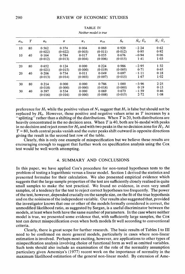
The results of the tests for T = 80 and T = 40 are given in Table IV. Experiments for T = 20 are not presented since these, in the vast majority of cases, gave a no decision result. Clearly, the sample size is very important in these experiments, as is the variability of the omitted variable. In all experiments, Ho is rejected much more frequently than is H1. The Sargan test, too, always favour H1 by a large majority. When T = 40, most experiments lead to no result with most of the remainder rejecting Ho only. However, when the sample size increases to 80, the test begins to reject both models, 6% of the time when U2, = 10, 22'4 per cent of the time when o2 = 20 and 78-6 per cent of the time when 0a2E = 30. Note that, in this case, the likelihood ratio favours H1 in all of the 500 cases so that the Sargan test, although decisive, is decisively wrong. Parenthetically, it is worth noting that the shifts in the distribution of No and N1 now appear to be much more complicated than when one of Ho and Hi was true. The negative values of No reflect the
290 REVIEW OF ECONOMIC STUDIES
TABLE IV
Neither model is true
0'2? T I IX 1 Io So N0:Vo N1:V1
10 80 0 562 0 374 0 004 0-060 0-920 -2 24 0 62 (0 022) (0 022) (0 003) (0 011) (0 012) 0 95 0 92
10 40 0 164 0 784 0 017 0 035 0-676 -0 94 0 06 (0 012) (0 013) (0 004) (0 006) (0 015) 1 41 1-03
20 80 0 652 0-124 0 000 0-224 0-986 -2 95 1 32 (0 021) (0 015) (0.000) (0 019) (0 005) 0 71 0 65
20 40 0 206 0 734 0 011 0 049 0-697 -1 11 0-18 (0-013) (0-014) (0.003) (0-007) (0 015) 1-67 1 02
30 80 0 214 0 000 0.000 0 786 1.000 -3 96 2 25 (0-018) (0 000) (0-000) (0.018) (0 000) 0.19 0 15
30 40 0 397 0 534 0 000 0 069 0 673 -1 59 0 46 (0 016) (0 016) (0 000) (0 008) (0.015) 2 72 1 08
preference for H1 while the positive values of N1 suggest that H1 is false but should not be replaced by Ho. However, these positive and negative values arise as T increases by a " splitting " rather than a shifting of the distributions. When T is 20, both distributions are heavily concentrated in the no decision area. When T is 40, both are bi-modal with peaks in no decision and reject zones for Ho and with two peaks in the no decision zone for H1. At T = 80, both central peaks vanish and the outer peaks shift outward in opposite directions giving the result in the second last row of the table.
Clearly, this is only one example of misspecification but we believe these results are encouraging enough to suggest that further work on specification analysis using the Cox test would be well worth attempting.
4. SUMMARY AND CONCLUSIONS
In this paper, we have applied Cox's procedure for non-tested hypotheses tests to the problem of testing a logarithmic versus a linear model. Section 1 derived the statistics and presented formulae for their calculation. We also presented empirical evidence which suggests that the large sample properties of the test are sufficiently closely realised in quite small samples to make the test practical. We found no evidence, in even very small samples, of a tendency for the test to reject correct hypotheses too frequently. The power of the test, however, depended crucially on the sample size, on the fit of the true hypothesis and on the noisiness of the independent variable. Our results also suggested that, provided the investigator knows that one or other of the models formally considered is correct, the unmodified likelihood ratio, as suggested by Sargan, is a useful discriminator between the models, at least when both have the same number of parameters. In the case where neither model is true, we presented some evidence that, with sufficiently large samples, the Cox test can detect misspecification even when both models fit well according to conventional criteria.
Clearly, there is great scope for further research. The basic results of Tables I to III need to be confirmed on more general models, particularly in cases where non-linear estimation is involved. Perhaps most exciting, however, are applications to other types of misspecification analysis involving choice of functional form as well as omitted variables. Such tests should also include an examination of the role of the normality assumption particulary given Amemiya's (1977) recent work on the importance of normality in the maximum likelihood estimation of the general non-linear model. By extension of Ame-
ANEURYN-EVANS & DEATON LINEAR VERSUS LOGARITHMIC 291
miya's results, it may turn out that while the Cox test is robust against non-normality when errors are additive, the robustness may not extend to the cases examined in this paper.
We should like to thank David Hendry, Adrian Pagan, Peter Phillips, Jean-Francois Richard, Gene Savin and especially Hashem Pesaran for extremely helpful comments. David Mitchell gave invaluable assistan6e with the computations.
REFERENCES AKAIKE, H. (1972), " Information theory and an extension of the maximum likelihood principle ", in Proc. 2nd
Int. Symp. on Information Theory, 267-281. AKAIKE, H. (1974), "A new look at the statistical model identification", IEEE Transactions on Automatic
Control, Ac-19, 716-723. AMEMIYA, T. (1973), " Regression analysis when the dependent variable is truncated normal ", Econometrica,
41, 997-1016. AMEMIYA, T. (1976), " Selection of regressors " (Stanford University Institute for Mathematical Studies in the
Social Sciences, Technical Report No. 225). AMEMIYA, T. (1977), "The maximum likelihood and the nonlinear three-stage least squares estimator in the
general non-linear simultaneous equation model", Econometrica, 45, 955-968. COX, D. R. (1961), " Tests of separate families of hypotheses " Proceedings of the Fourth Berkeley Symposium on
Mathematical Statistics and Probability 1, (Berkeley: University of California Press). COX, D. R. (1962), " Further results on tests of separate families of hypotheses ", Journal of the Royal Statistical
Society Series B, 24, 406424. EDWARDS, A. W. F. (1972) Likelihood (Cambridge University Press). MIZON, G. E. and HENDRY, D. F. (1980), "An empirical application and Monte Carlo analysis of tests of
dynamic specification", Review of Economic Studies, (this issue). PESARAN, M. H. (1974), "On the general problem of model selection", Review of Economic Studies 41,
153-171. PESARAN, M. H. and DEATON, A. S. (1978), "Testing non-nested non-linear regression models",
Econometrica, 46, 677-694. QUANDT, R. E. (1974), "A comparison of methods for testing non-nested hypotheses ", Review of Economics
and Statistics, 56, 92-99. SARGAN, J. D. (1964), "Wages and prices in the United Kingdom ", in Hart, P. E., Mills, G. and Whitaker, J. K.
(eds.) Econometric Analysis for National Economic Planning (London: Butterworths). SAWA, T. (1978), "Information criteria for discriminating among alternative regression models",
Econometrica, 46, 1273-1291.