eviews handout 2010 - julius.csscr.washington.edujulius.csscr.washington.edu/pdf/eviews...

EViews Document CSSCR Fall 2010 Updated by Jianguo Wang

1

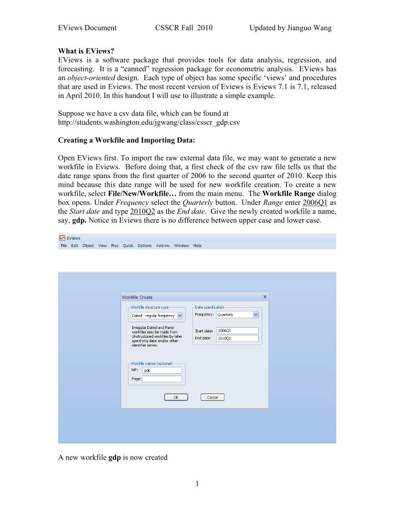
What is EViews? EViews is a software package that provides tools for data analysis, regression, and forecasting. It is a “canned” regression package for econometric analysis. EViews has an object-oriented design. Each type of object has some specific ‘views’ and procedures that are used in Eviews. The most recent version of Eviews is Eviews 7.1 is 7.1, released in April 2010. In this handout I will use to illustrate a simple example. Suppose we have a csv data file, which can be found at http://students.washington.edu/jgwang/class/csscr_gdp.csv Creating a Workfile and Importing Data: Open EViews first. To import the raw external data file, we may want to generate a new workfile in Eviews. Before doing that, a first check of the csv raw file tells us that the date range spans from the first quarter of 2006 to the second quarter of 2010. Keep this mind because this date range will be used for new workfile creation. To create a new workfile, select File/New/Workfile… from the main menu. The Workfile Range dialog box opens. Under Frequency select the Quarterly button. Under Range enter 2006Q1 as the Start date and type 2010Q2 as the End date. Give the newly created workfile a name, say, gdp. Notice in Eviews there is no difference between upper case and lower case.

A new workfile gdp is now created


2

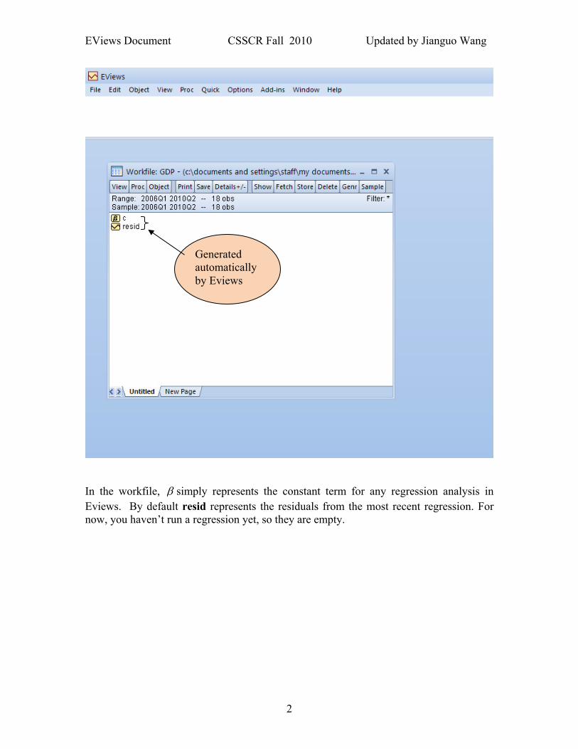
In the workfile, β simply represents the constant term for any regression analysis in Eviews. By default resid represents the residuals from the most recent regression. For now, you haven’t run a regression yet, so they are empty.

Generated automatically by Eviews


3

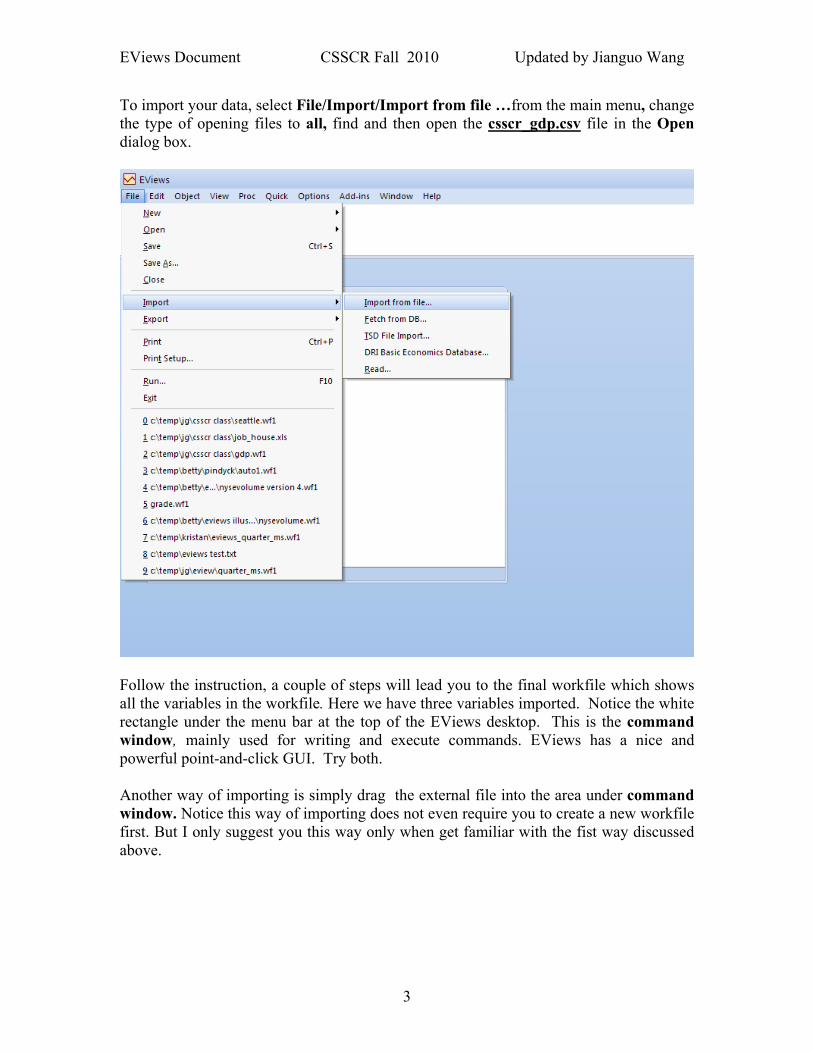
To import your data, select File/Import/Import from file …from the main menu, change the type of opening files to all, find and then open the csscr_gdp.csv file in the Open dialog box.

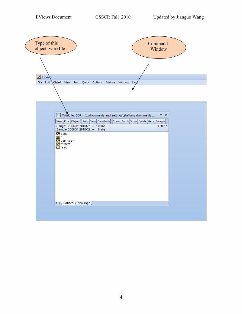
Follow the instruction, a couple of steps will lead you to the final workfile which shows all the variables in the workfile. Here we have three variables imported. Notice the white rectangle under the menu bar at the top of the EViews desktop. This is the command window, mainly used for writing and execute commands. EViews has a nice and powerful point-and-click GUI. Try both. Another way of importing is simply drag the external file into the area under command window. Notice this way of importing does not even require you to create a new workfile first. But I only suggest you this way only when get familiar with the fist way discussed above.


4

Type of this object: workfile

Command Window


5

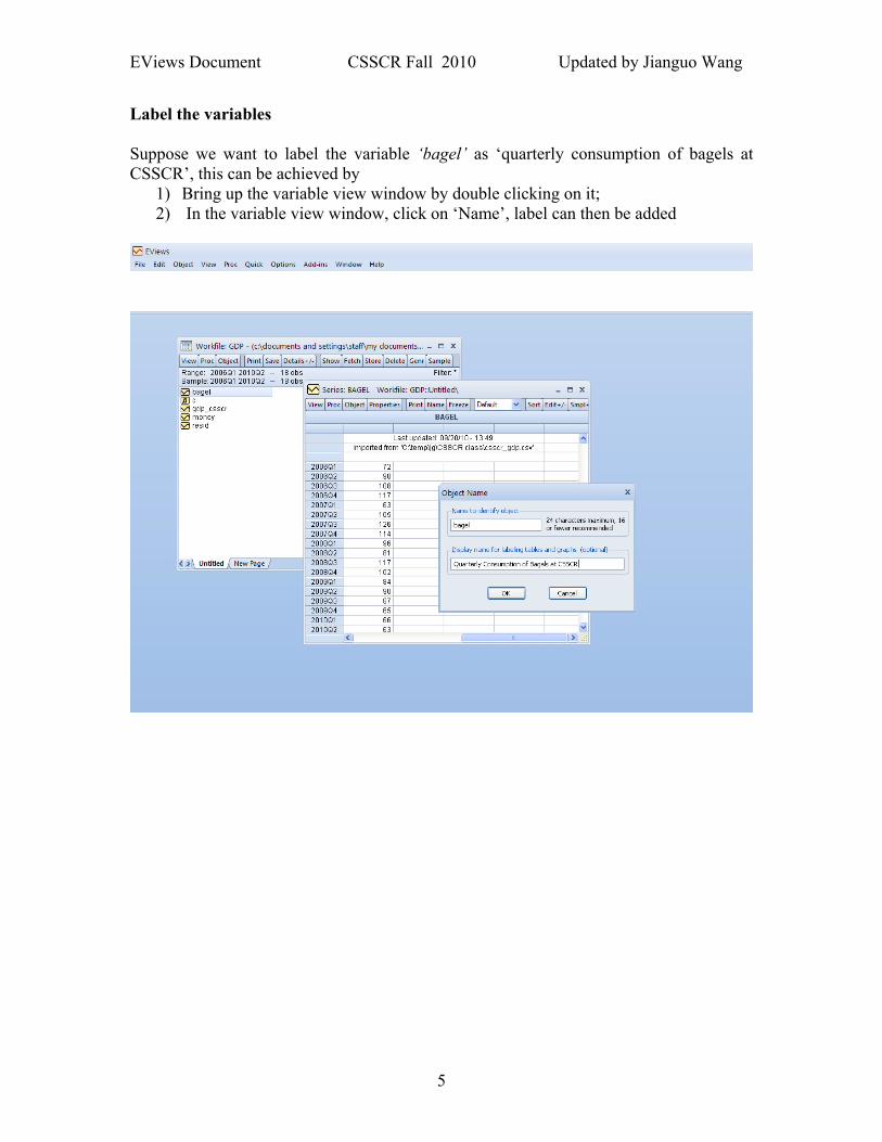
Label the variables Suppose we want to label the variable ‘bagel’ as ‘quarterly consumption of bagels at CSSCR’, this can be achieved by

1) Bring up the variable view window by double clicking on it; 2) In the variable view window, click on ‘Name’, label can then be added


6

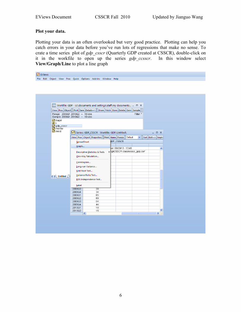
Plot your data. Plotting your data is an often overlooked but very good practice. Plotting can help you catch errors in your data before you’ve run lots of regressions that make no sense. To crate a time series plot of gdp_csscr (Quarterly GDP created at CSSCR), double-click on it in the workfile to open up the series gdp_ccsscr. In this window select View/Graph/Line to plot a line graph


7

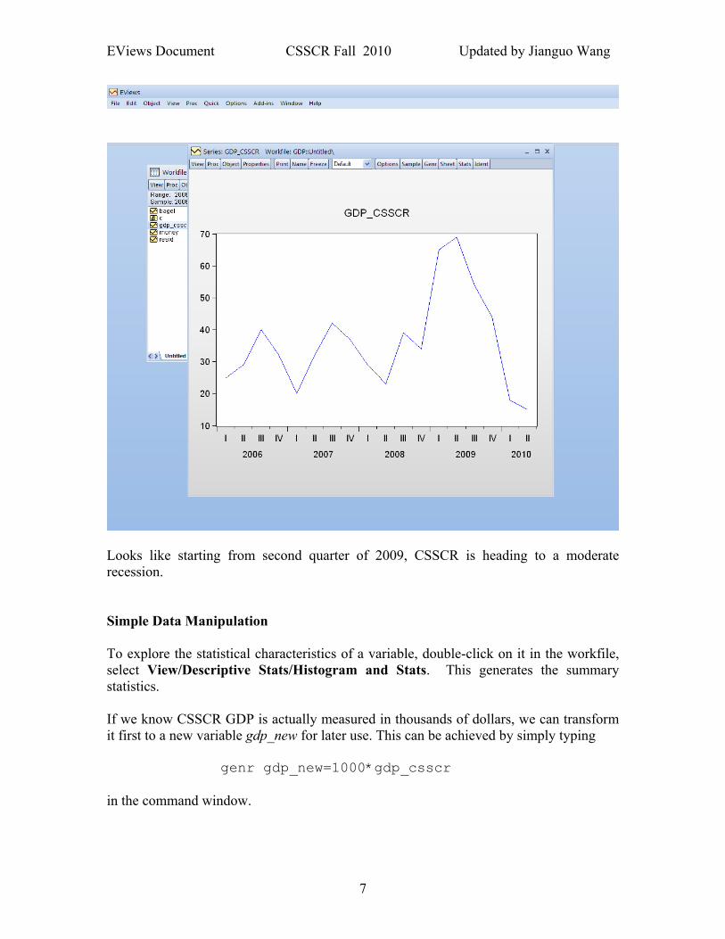
Looks like starting from second quarter of 2009, CSSCR is heading to a moderate recession. Simple Data Manipulation To explore the statistical characteristics of a variable, double-click on it in the workfile, select View/Descriptive Stats/Histogram and Stats. This generates the summary statistics. If we know CSSCR GDP is actually measured in thousands of dollars, we can transform it first to a new variable gdp_new for later use. This can be achieved by simply typing genr gdp_new=1000*gdp_csscr in the command window.


8

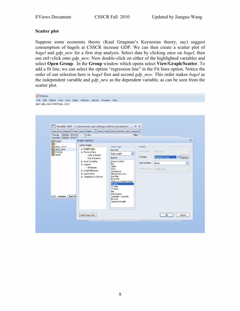
Scatter plot Suppose some economic theory (Kaul Grugman’s Keynesian theory, say) suggest consumption of bagels at CSSCR increase GDP. We can then create a scatter plot of bagel and gdp_new for a first step analysis. Select data by clicking once on bagel, then use ctrl+click onto gdp_new. Now double-click on either of the highlighted variables and select Open Group. In the Group window which opens select View/Graph/Scatter. To add a fit line, we can select the option “regression line” in the Fit lines option. Notice the order of our selection here is bagel first and second gdp_new. This order makes bagel as the independent variable and gdp_new as the dependent variable, as can be seen from the scatter plot.


9

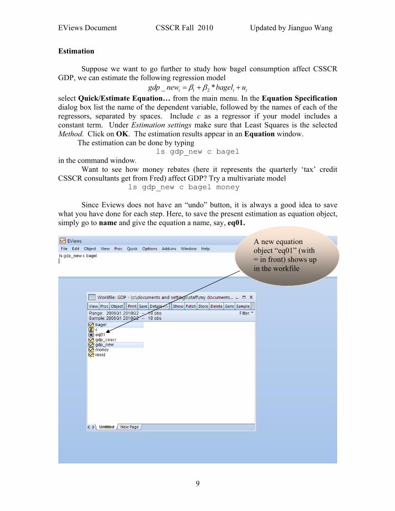
Estimation

Suppose we want to go further to study how bagel consumption affect CSSCR GDP, we can estimate the following regression model _ *t t tgdp new bagel uβ β1 2= + + select Quick/Estimate Equation… from the main menu. In the Equation Specification dialog box list the name of the dependent variable, followed by the names of each of the regressors, separated by spaces. Include c as a regressor if your model includes a constant term. Under Estimation settings make sure that Least Squares is the selected Method. Click on OK. The estimation results appear in an Equation window. The estimation can be done by typing

ls gdp_new c bagel in the command window. Want to see how money rebates (here it represents the quarterly ‘tax’ credit CSSCR consultants get from Fred) affect GDP? Try a multivariate model

ls gdp_new c bagel money

Since Eviews does not have an “undo” button, it is always a good idea to save what you have done for each step. Here, to save the present estimation as equation object, simply go to name and give the equation a name, say, eq01.

A new equation object “eq01” (with = in front) shows up in the workfile


10

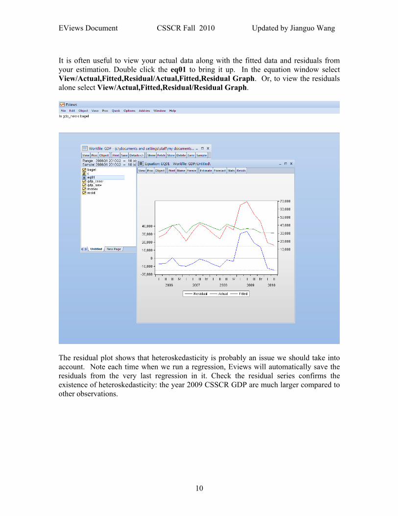
It is often useful to view your actual data along with the fitted data and residuals from your estimation. Double click the eq01 to bring it up. In the equation window select View/Actual,Fitted,Residual/Actual,Fitted,Residual Graph. Or, to view the residuals alone select View/Actual,Fitted,Residual/Residual Graph.

The residual plot shows that heteroskedasticity is probably an issue we should take into account. Note each time when we run a regression, Eviews will automatically save the residuals from the very last regression in it. Check the residual series confirms the existence of heteroskedasticity: the year 2009 CSSCR GDP are much larger compared to other observations.


11

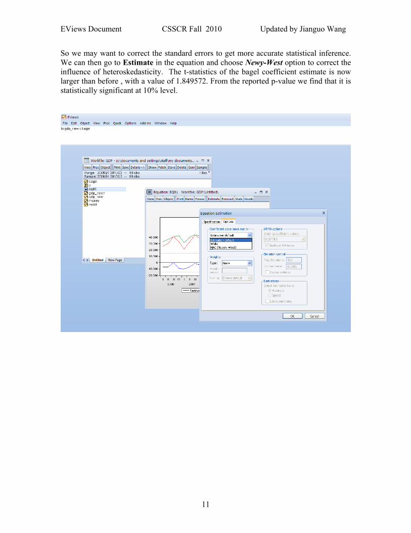
So we may want to correct the standard errors to get more accurate statistical inference. We can then go to Estimate in the equation and choose Newy-West option to correct the influence of heteroskedasticity. The t-statistics of the bagel coefficient estimate is now larger than before , with a value of 1.849572. From the reported p-value we find that it is statistically significant at 10% level.


12

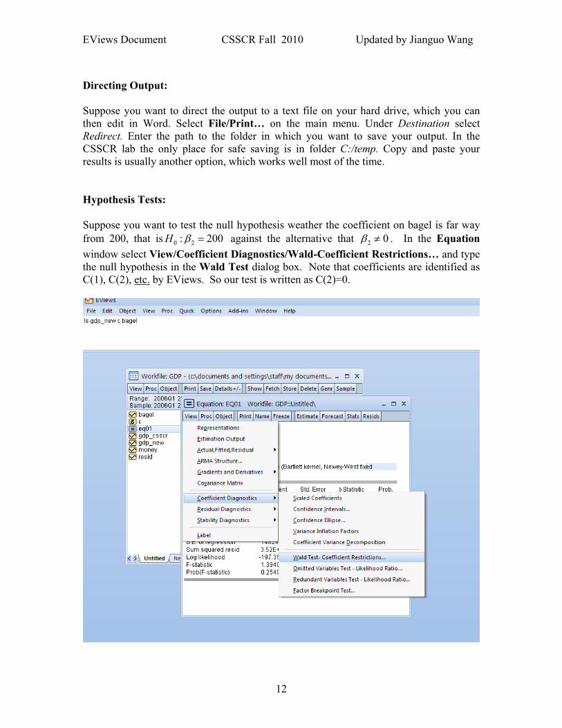
Directing Output: Suppose you want to direct the output to a text file on your hard drive, which you can then edit in Word. Select File/Print… on the main menu. Under Destination select Redirect. Enter the path to the folder in which you want to save your output. In the CSSCR lab the only place for safe saving is in folder C:/temp. Copy and paste your results is usually another option, which works well most of the time. Hypothesis Tests: Suppose you want to test the null hypothesis weather the coefficient on bagel is far way from 200, that is 0 2: 200H β = against the alternative that 2 0β ≠ . In the Equation window select View/Coefficient Diagnostics/Wald-Coefficient Restrictions… and type the null hypothesis in the Wald Test dialog box. Note that coefficients are identified as C(1), C(2), etc. by EViews. So our test is written as C(2)=0.


13

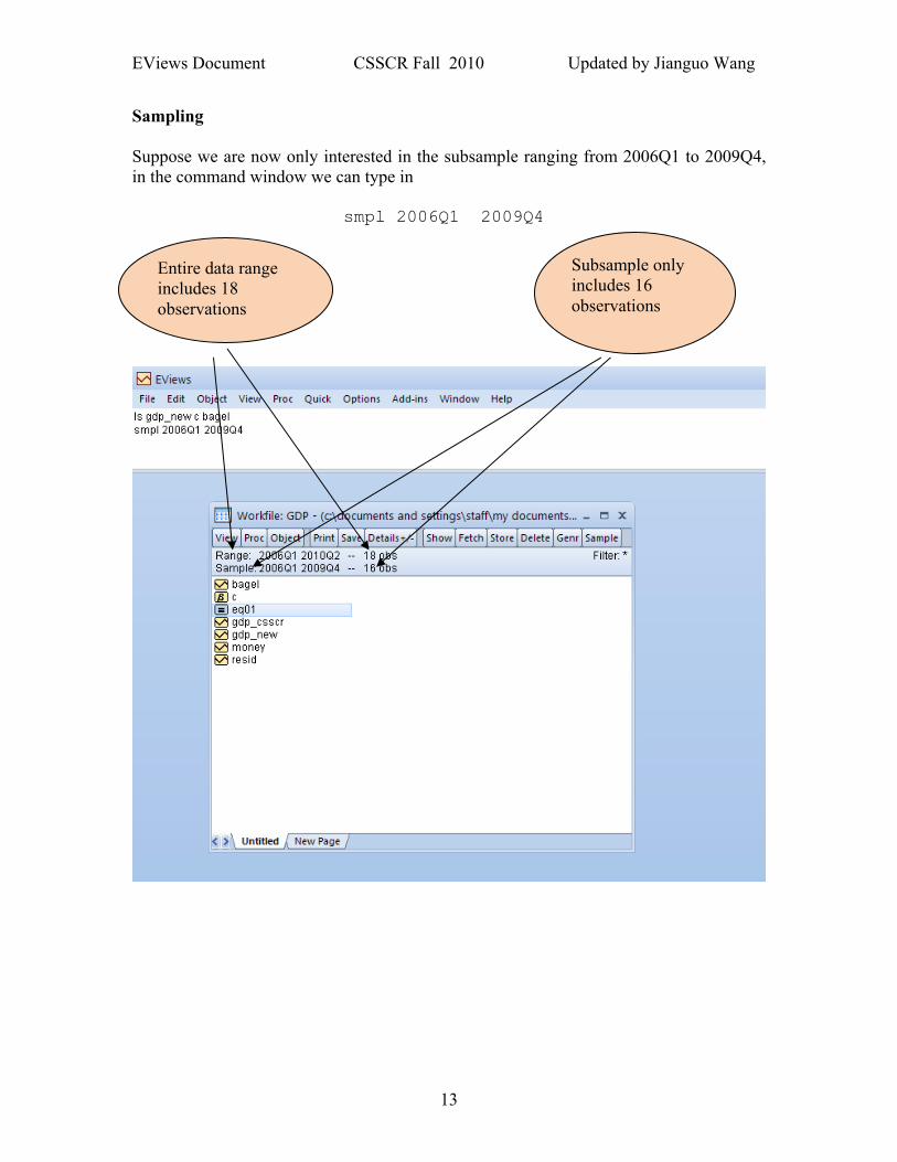
Sampling Suppose we are now only interested in the subsample ranging from 2006Q1 to 2009Q4, in the command window we can type in

smpl 2006Q1 2009Q4

Entire data range includes 18 observations

Subsample only includes 16 observations


14

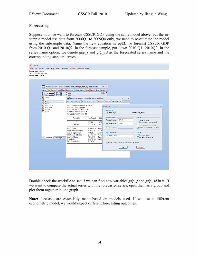
Forecasting Suppose now we want to forecast CSSCR GDP using the same model above, but the in- sample model use data from 2006Q1 to 2009Q4 only, we need to re-estimate the model using the subsample data. Name the new equation as eq02. To forecast CSSCR GDP from 2010 Q1 and 2010Q2, in the forecast sample, put down 2010 Q1 2010Q2. In the series name option, we denote gdp_f and gdp_sd as the forecasted series name and the corresponding standard errors.

Double check the workfile to see if we can find new variables gdp_f and gdp_sd in it. If we want to compare the actual series with the forecasted series, open them as a group and plot them together in one graph. Note: forecasts are essentially made based on models used. If we use a different econometric model, we would expect different forecasting outcomes.


15

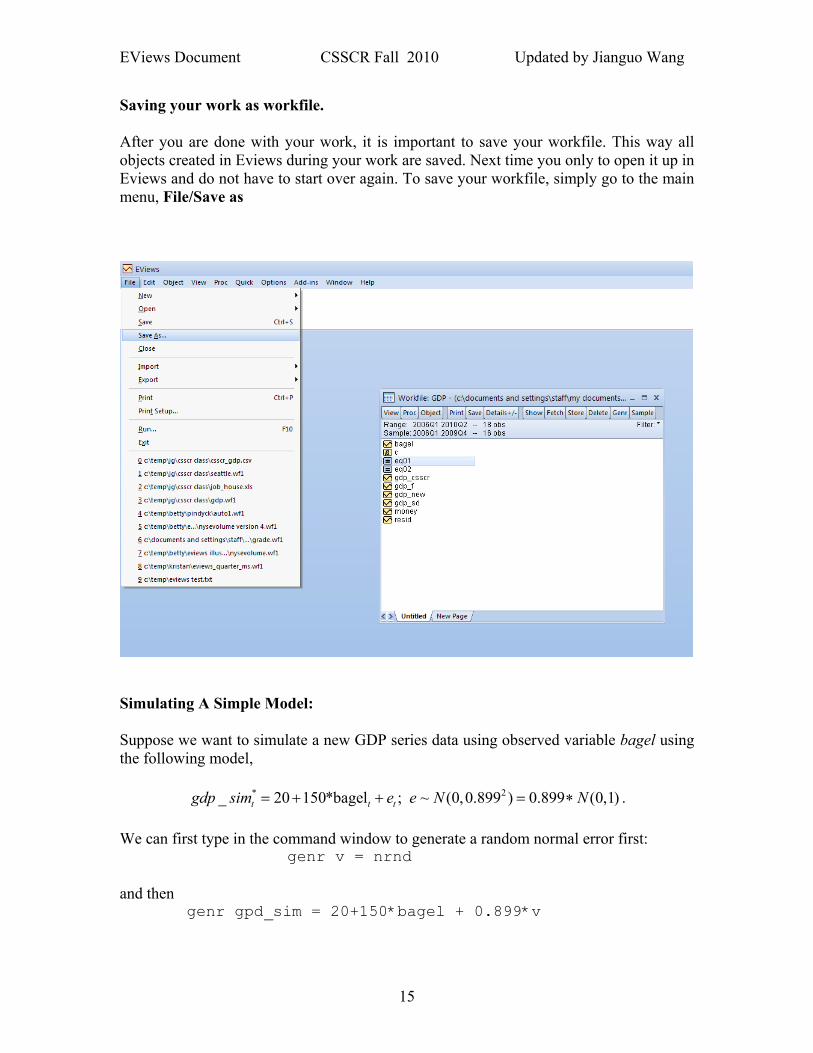
Saving your work as workfile. After you are done with your work, it is important to save your workfile. This way all objects created in Eviews during your work are saved. Next time you only to open it up in Eviews and do not have to start over again. To save your workfile, simply go to the main menu, File/Save as

Simulating A Simple Model: Suppose we want to simulate a new GDP series data using observed variable bagel using the following model, * 2_ 20 150*bagel ; ~ (0,0.899 ) 0.899 (0,1)t t tgdp sim e e N N= + + = ∗ . We can first type in the command window to generate a random normal error first: genr v = nrnd and then

genr gpd_sim = 20+150*bagel + 0.899*v


16

Appdendix:

1) Commonly used objects in Eviews Some basic objects: Workfile, Series/variables, Groups, Graphs, Equations. More advanced objects: system of equations, VAR , State Space Models, etc.

2) Some Useful EVIEWS commands

Sample Handling in Eivews For time series data, understanding Date formats (see also Help/Search/Dates) in Eviews is important for sample handling. EViews uses dates to identify time periods. Rules for composing dates are: Annual: the full year, for example, 1981, 1895, 2001 Quarterly: the full year or the last two digits of the year, colon, and the quarter number. Examples: 1992:1, 65:4, 2002:3. Monthly: the full year or the last two digits of the year, colon, and the month number. Examples: 1956:1, 1990:11,1997M10. Weekly and daily: Month number, colon, day number, colon, and year. For weekly data, the week is identified by the first day of the week. Example: 3:10:87 is March 10, 1987 or the week starting that day. Suppose we only want to studying the relation between d_price and unemployment during the time period from smpl 1995M1 2000M12 All the following operations in Eviews all only apply to this sample period. After you are done with this sample period’s work, it is a good habit to always reselect the entire sample period for future work. To do that, simly type into the command window the following smpl @all or smpl @first @end


17

Resources http://julius.csscr.washington.edu/ http://forums.eviews.com/

eviews handout 2010 - julius.csscr.washington.edujulius.csscr.washington.edu/pdf/eviews...

Documents