r I AV-2 439 L___----J

le% ASATzt± MILITARY TECHNICAL COLLEGE

CAIRO - EGYPT

1

SYSTEM IDENTIFICATION USING MODIFIED

LMS ADAPTIVE RECURSIVE FILTERING ALGORITHM

BY E. A. SOLEIT

* CPh. D)

ABSTRACT

The application of the adaptive filtering techniques in system identification and control has received a great interest to model an unknown plant based on the minimisation of the mean square error criterion. Any physical system is well represented by an auto-regressive moving average transfer function. Hence, the infinite impulse response adaptive filter is able to match a zero-pole transfer function with fewer number of coefficients. In this paper a new adaptation algorithm is introduced to update the forward and the backward filter coefficients. The proposed adaptive filter matches efficiently the unknown systems which are modeled by all pole and zero-pole transfer functions. The filter coefficients have converged exactly to the optimal values.

* Lecturer in the a': ground securing department. Military

Technical College, Cairo. Egypt.

AV-2440. ===.17‘30011..

INO0

MILITARY TECUNICAL COLLEGE

CAIRO - EGYPT

I. Introduction

Modeling and system identification are very important in the field of control, communication and signal processing(1). The unknown plant and the adaptive identifier have the same observation inputs. The coefficients of the identifier are adjusted such that a mean square error ,performance criterion is minimized. Moreover, an adaptation algorithm is used to update the identifier coefficients and to track any variation of the unknown plant (21.

The physical systems are represented by an auto regressive moving average ( ARNA ) transfer function. ience. the adaptive recursive filter is the best example to model the physical systems. A proposed least mean square (MS) adaptation algorithm is introduced to update the recursive filter coefficients (31. In this algorithm, the gradient vector is liberalized and is calculated by a moving average process rather than by an auto regressive one as in White and St earns algorithms (4,51 Hence, the stability of the proposed algorithm has been improved for a wide range of step size parameter during the adaptation process.The performance measures of the introduced adaptation algorithm are examined by computer simulation.

This paper has five sections. Section two explains the formulation analysis of the adaptive identifier. The proposed MS adaptation algorithm is introduced in section three. Section four demonstrates tl,e simulation results. Conclusions are given in section five

HI- System formulation

The identification of an unknown plant using the adaptive filtering technique is depicted in Figure 1. The coefficients of the adaptive filter are adjusted such that. the mean square of the error signal, ek is minimized. In this case.the adaptive filter

represents a good model of the unknown system:The unknown system is represented by an auto regressive moving average transfer function, then. the output signal, dk can be expressed generally

as (6):

N M

it) d - E ax- +rbd k k ki - J -J

1-0 i-i Equation (1) can be written in matrix form as:

dk m ATxk BTDk (2)

where X and Dk ars tfie input and output observation vectors

respectively and are defined as:

Xk ( xk xk-N

) (3)

and

$ 1 AV-2 '441 1

MILITARY TLCHNICAL CuLLEGE

CAIRO - EGYPT

1

Dk (dk-1 dk-2 dk-M 1 (4)

The forward and the backward coefficient vectors, A and B are defined respectively as:

AT= ( a0 a1 a2 aN ) (5) and

T B = Ha1 b2 b

M ( 6)

The output of the adaptive recursive filter, yk can be written as:

Lf Lb

Yk = E ai,k xk-i E bj.k yk-j (7)

j-1 or in matrix notation as (7]:

T T Yk = ak Sk Yk (8)

where Sk and Yk are the input and output observation vectors

respectively and are defined as:

Sk - [ xk xk-1 xk-Lf

and

Yk Yk-1 Yk-2"' c10) Yk-Lbi ak and yk are the forward and the backward coefficient vectors of

the adaptive filter. They are defined respectively as:

a0,k 81,k aLf'k (11)

and

T rk [bI,k b2.k bI"b' k)

(1y2) The error signal, ek is defined as:

ek = dk - yk (13)

Substituting (2) and (8) in (13) yields:

ck = ( AT Xk akT Sk ) + ( BT Dk - rk Yk ) (14)

(15)

The error signal, ek in (14) can be written as:

ek ef.k h,lc

where ef,k and. E'b,k

AT X

are defined respectively as:

S. (16) and

--7=-----7---A S A Tiz- MILITARY TECHNICAL COLLEGE

CAIRO - EGYPT

K Dk (17)

111- The adaptation algorithm

filter coefficients are updated such that the mean square E r'' j is minimized. During the adaptation process, the

2 -1-Ive'ea E

k ] is replaced by the instantaneous squared

1-or signal, (8). The gradient based adaptation algorithm is

4:.1 to update the forward and the backward coefficients. The E4p est decent adaptation algorithm is defined in [9] as:

),(41 = ak - p Vf (18)

(Id

Yk+1 Yk 71) (19)

where arid Vb are the gradient vectors with respect to the

forward. and the backward coefficients respectively. p is the step size parameter that controls Lhe convergence rate and the 7;t3bi ity 1 the adaptation algorithm [10]. The forward gradient vector f can be expressed as:

=

(20)

bstitnting (1) in (20) the forward gradient vector becomes:

cf,k eb,k - 4-

ak a ak

(21)

Substituting (16) and (17) in (21) Of can be written

as

Of = - 2 rk ( S1, (22)

where the derivative matrix Tk is defined as

Yk

(23)

a clk

Similarly, the backward gradient vector, Vb can be expressed as :

I _1 AV-2 443

AB A TE--- MILITARY TECHNICAL COLLEGE

CAIRO - EGYPT

b - 2 ( Yk + lk rk )

(24)

where the derivative matrix

is expressed as:

8 Yk

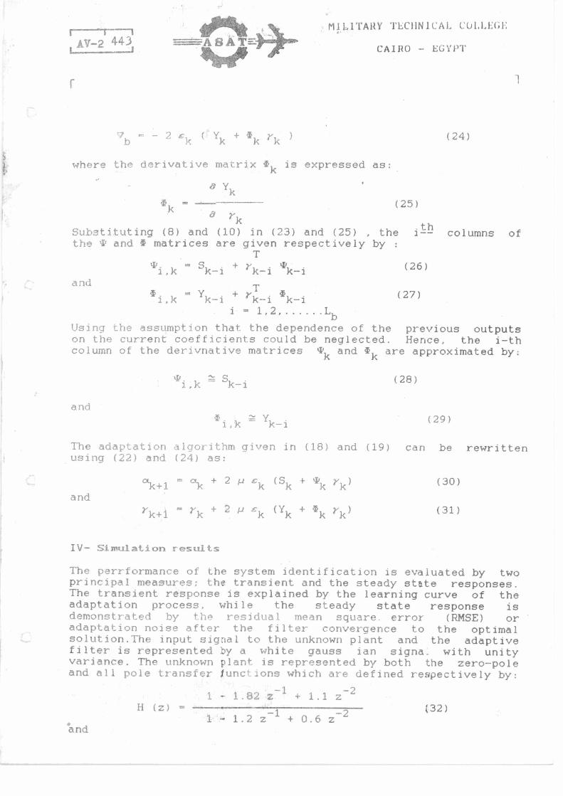
Substituting (8) and (10) in (23) and (25) , the 1-- .th columns of

the W and 1 matrices are given respectively by : T

i.k Sk-i+ . k-1 k-1

T . (26)

1.k k-1 + § k-1 k-i (27) i = 1,2 Lb

Using the assumption that the dependence of the previous outputs on the current coefficients could be neglected. Hence, the i-th column of the derivnative matrices T

k and tk are approximated by:

T.1 S,k k -i

and .

1,k k -1

The adaptation algorithm given in (18) and (19) can be rewritten using (22) and (24) as:

ak+1 = ak 2 u (Sk Ikk rk) (30)

and

rk+1 = rk 2 (Yk lk rk)

(31)

IV- Simulation results

The perrformance of the system identification is evaluated by two

The transient response is explained by the learning curve of the principal measures; the transient and the steady state responses.

adaptation process, while the steady state response is demonstrated by the residual mean square. error (RMSE) or adaptation noise after the filter convergence to the optimal solution.The input signal to the unknown plant and the adaptive filter is represented by a white gauss ian signa. with unity variance. The unknown plant is represented by both the zero-pole and all pole transfer functions which are defined respectively by:

1 - 1.82 z-1 + 1.1 z-2

H (z) -

(32) 1 - 1.2 z-1 + 0.6 z-2

and

k 8 rk (25)

and

(28)

(29)

I le% MILITARY T1', L CHNICAL CO LEE (;

AV-2I 444 AlSiVr=4■)H

1 *be

CA1R0 - EGYPT

1 II (z) (33)

1 - 1.2 z-1 + 0.6 z

-2

The learning curve illustrates the change of the instantaneous mean square error versus the iteration number, k (sampling intervals ) It is measured by ensemble averaging of 16 individual learning curves. The learning curves of the zero-pole (Nf = 3 and

Nb 2 ) and all pole (Nf

= 1 and Nb = 2)adaptive recursive filters

are shown in Figure 2 and 3 respectively. It is concluded that the zero-pole filter has a higher convergence rate than that of the all pole filter. On the other-hand, the all pole filter has smaller adaptation noise (maladjustment) than that of the zero-pole filter after convergence.

The residual mean square error ( RMSE ) is measured after 5168 iterations. over a period of 2000 samples. The RMSE is defined as:

RMSE - 1 7168 2 E 2000 j=91683

The RMSE defined in (34)is measured versus a design parameter M that is defined by :

M = P( Nf + N

b ) (35)

where Nf and Nb

are the numbers of the forward and the backward

coefficients respectively. The RMSE versus M for the zero-pole and all pole adaptive filters are depicted in Figures 4 and 5 respectively. Figure 4 illustrates that the zero-pole filter has nearly zero RMSE as 0.02 5 M IC 0.2. If M increases above 0.2 , the RMSE increases significantly. Moreover, Figure 5 explains that the all -pole filter has RMSE nearly zero as 0.01 M :5 0.07. The RMSE increases as M increases above 0.07. It is concluded from Figure 4 and 5 that the pole-zero adaptive recursive filter has greater range of M ( step size ) over the all pole filter, to ensure filter convergence and to .attain a small adaptation noise. Furthermore, the adaptive filter coefficients converge exactly to the optimal values. The forward and the backward coefficients of both the unknowW'plant and the adaptive filter after convergence are listed in Table 1.

V- Conclusion

The adoptivfi iecninive tiller can match efficiently a phynical unknown system. . The transient and the steady state responses of the adaptive filter depends on its structure. The zeros addition improves the convergence property and decreases the fluctuations during the transient time.The zero--pole filter converges and remains stable for great range of step sizes while the stability and convergence of the.all pole filter is restricted to a smaller range of step sizes.The proposed adaptation algorithm ensures the convergence of ,the filter coefficients to the optimal values.

r----r---1 AV-2 445

MILITAIL: TECHNICAL COLL177GE

CAIRO - EGYPT

VI- References

[1) Widrow B. and Stearns S. D. " Adaptive signal processing Prentice Hall Inc, Englewood, 1985.

[2] Cowan C. F. and et al. " Adaptive filters, Prentice Hall. New Jersy, 1985.

[31 Soleit E. A. " Adaptive digital filter algorithms and their application to echo cancellation ". Ph. D dissertation, Elect.Eng. Department, UKC., U.K, 1989.

14) White S. A., " An adaptive recursive filter ", Annual Asilomar Con. Circuit and Systems„ San Francisco. pp.21-25. Nov. 1975.

[5] Stearns S. D. and Elliot G. R., " On adaptive recursive filtering ", Proceedings of 12-th Asilomar Con. Circuits, System and Computer, Pacific Grove. pp. 5•10, Nov. 1976.

[6] Friedlander B., " System identification techniques for adaptive signal processing ", Circuit Systems Signal process, vol. 1, No. 1, 1982.

[7] Feintuch P. L., " An adaptive recursive MS filter ". Proc. IEEE, vol. 64. pp. 1622-1624., Nov. 1976.

[8) Widrow B. and McCool J., " A comparison of adaptive algorithms based on the methods of steepest descent and random search ", Tarns. on antenna and propagation, vol. AP-24, pp. 615-636, Sep. 1976.

(9) Scales L., " Introduction to non-linear optimization ", London, 1986.

[10] Feuer A. and Weinstein E., Convergence analysis of LMS filter with uncorrected gaussian data ", IEEE Tarns.ASP. vol-33, pp.222-229, Feb. 1985.

Input signal

x K

a2 44-

MILITARY TECHNICia. COLLEGE

CAIRO — EGYPT

Figure 1 The adaptive system identification model

Table 1 The Forward and the backward coefficients after convergence ( E1 = 0.02 )

Unknown The filter system Pole-zero All pole

pole all coefficients

zero pole filter filter

ao 1.0 1.0 0.999999 1.0

a 1 -1.82 -1.81999

a t 1.1 1.099999

b,

bl

1.2

-0.6

1.2

-0.6

1.199999

0,599999

1.2

-0.6

1 8 142

8 C2

CCr-4

8 8 8. 8 8° • n ao8a3 3eltenOSINUM

N

O

II 6 •44 14 V ✓

_X 0

ptl

$ 2

✓ 0

V

I

I

I ••i,•■•

3S1,48

FOURTH ASAT CONFERENCE

14-16 May 1991 , CAIRO AV-2 44T

•

pM

.44

04

✓

O

4

5

a 8 9 80

0 0 3S;,"vd

'gm

0

J tl

a I

O

O

•

✓

ti

•••

• '

0

4

_ m • •

60 •4. P.

0 0

1 a tl

64

0

0 0 se 0 ✓

O

4

V 0 pM O

8 8 . N

d0863 aftenos NV311