quikslope manual module 1 - members.iinet.net.aumembers.iinet.net.au/~softrock/support/module 1 -...

QuikSlope Manual

May 2010, QuikSlope Manual Version 3.0

Copyright © SoftRock Solutions Pty Ltd 2010 All Rights Reserved

QuikSlope Manual Module 1

QuikSlope Manual Version 3.0 Software Version 4.677

SoftRock Solutions specialise in slope monitoring. We have developed software and systems that will assist you with your slope monitoring needs.

QuikSlope Manual

2 / 148

May 2010, QuikSlope Manual Version 3.0 Copyright © SoftRock Solutions Pty Ltd 2010 All Rights Reserved

SoftRock Manuals Overview

SoftRock has produced a range of manuals to assist the user of its systems and software to gain the most from these products. Each manual has a unique numbering system, which allows for easy cross-referencing:

Module Number Content Module 1 QuikSlope Manual Module 2 AutoSlope Manual Module 3 Quikcom Manual Module 4 SoftRock Automated site – At A Glance Module 5 AutoSlope Installation Manual Module 6 Leica Onboard Slope Monitoring Manual Module 7 FieldSat Manual Module 8 AutoSat Manual Module 9 ATS Pocket PC Manual Module 10 Analyzer Manual

A quick example of cross-referencing

Module 2 AutoSlope Manual Index number 2.15.3.1 Instrument Settings Refers to Module 2; Chapter 15; Section 3,

Subsection 1. This cross-referencing scheme can be easily be used across any SoftRock manual. For example in Module 1 QuikSlope Manual, 1.2.1.4 Database creation. We regularly make use of cross-referencing to other manuals within our software collection. This avoids repetition, makes for easy updating, and provides an efficient method to record information. It is therefore important that the user understands this unique numbering system, as all the information for our programs cannot fit into a single manual.

QuikSlope Manual

3 / 148


Contents

Contents........................................................................................................... 3

Important Note - Date Format ....................................................................... 7

Part A Overview of Quikslope ...................................................................... 9 1.0 Field Data ............................................................................................................9 1.0.1 Calculations ....................................................................................................10 1.0.2 Base Reading..................................................................................................11 1.0.3 Reporting ........................................................................................................11 1.0.4 Excel Spreadsheet ..........................................................................................12

Part B QuikSlope Main Menu...................................................................... 13 1.1 Toolbar...............................................................................................................13 1.1.0 File ..................................................................................................................13

1.1.1 New Project.................................................................................... 13 1.1.2 Open Project .................................................................................. 14 1.1.3 Current Picture............................................................................... 14 1.1.4 Current Configuration Directory.................................................... 14

1.2 Data Import........................................................................................................15 1.2.1 Geodimeter, Leica, Topcon, Sokkia and Nikon ........................... 15 1.2.2 Import Qslope Vers 0.9 Data ........................................................ 17 1.2.3 Import Coordinate only Data ......................................................... 17 1.2.4 Data Structure................................................................................ 18

1.3 Edit .....................................................................................................................22 1.3.1 Edit Setup Data.............................................................................. 22 1.3.2 Edit Prism Data .............................................................................. 23 1.3.3 Delete Data .................................................................................... 26 1.3.6 Edit Area Names............................................................................ 28 1.3.7 Edit Bench Marks........................................................................... 29 1.3.8 Edit Events ..................................................................................... 32 1.3.9 Edit Prism Name............................................................................ 33 1.3.10 Rainfall.......................................................................................... 35

QuikSlope Manual

4 / 148


1.3.11 Crack Monitors............................................................................. 36 1.3.12 Seismic Activity ............................................................................ 38

1.4 Calculations .......................................................................................................40 1.4.1 Calculate Co-ordinates.................................................................. 41 1.4.2 Survey Control Database .............................................................. 48 1.4.3 Recalculate Movements ................................................................ 51 1.4.4 Global Calculations........................................................................ 53

1.5 Reporting and Exporting ..................................................................................57 1.5.1 Prism Graphing .............................................................................. 58 1.5.2 Prism Reports .............................................................................. 101 1.5.3 Create Export File for Spreadsheets .......................................... 104 1.5.4 Export Plot Data File (Surpac) .................................................... 109

1.6 Database Utility...............................................................................................113 1.6.1 Cropping and Exporting .............................................................. 114 1.6.2 Database Integrity Check............................................................ 117 1.6.3 Pack Database............................................................................. 117 1.6.4 Repair Database.......................................................................... 117 1.6.5 Remove all Crest and Toe Lines ................................................ 118

1.7 Help..................................................................................................................118 1.7.1 About ............................................................................................ 118 1.7.3 Register Software ........................................................................ 119

Part C QuikSlope - First User Guide........................................................ 120 1.8 First Time Check List .....................................................................................120

1.8.1 Field Procedures (Manually) ....................................................... 121 1.8.2 Field Data ..................................................................................... 121 1.8.3 Edit Data....................................................................................... 123 1.8.4 Setup Data ................................................................................... 126 1.8.5 Calculate Coordinates ................................................................. 126 1.8.6 Calculation Procedure ................................................................. 127 1.8.7 Setup Station Data ...................................................................... 127 1.8.8 Control Coordinates..................................................................... 128 1.8.9 Target Base Readings................................................................. 130 1.8.10 Reporting-Printouts.................................................................... 131 1.8.11 Creating CSV File...................................................................... 133 1.8.12 Excel and QuikSlope ................................................................. 134

QuikSlope Manual

5 / 148


Part D Terminology .................................................................................... 135 1.9 Graphing Terminology ...................................................................................135

1.9.1 XYZ Movement ............................................................................ 135 1.9.2 XYZ Vector Movement ............................................................... 135 1.9.3 Unadjusted Distance .................................................................. 135 1.9.4 Adjusted Field Data ..................................................................... 135 1.9.5 Adjusted Distance....................................................................... 136 1.9.6 Distance and Adjustment Factor ............................................... 136 1.9.7 7 Day Velocity .............................................................................. 137 1.9.8 30 Day Velocity ........................................................................... 137 1.9.9 90 Day Velocity ........................................................................... 137

1.10 QuikSlope Terminology ...............................................................................138 1.10.1 Reference Prism........................................................................ 138 1.10.2 Benchmark ................................................................................ 138 1.10.3 Setup Number........................................................................... 138 1.10.4 Target ID ................................................................................... 139 1.10.5 Area Name................................................................................ 139

1.11 Instruments ....................................................................................................140 1.11.1 Robotic Instruments ................................................................. 140 1.11.2 Topcon Data Format ................................................................ 140 1.11.3 Wild Leica File Format ............................................................. 141 1.11.4 Geodimeter File Format ........................................................... 142 1.11.5 Geodimeter Servo Driven Procedures .................................... 143

Appendix Diagrams.................................................................................... 146

QuikSlope Manual

6 / 148


Release Information

Prepared By : Harsha Seneviratne (HS) Reviewed By : Bernie Malone (BM) Authorised By : Bernie Malone

Configuration History Version No. Date Change Details Author 1 Initial Draft BM

2 01/03/09 Update BM

3 10/05/10 Upgrade to new template

HS

Distribution Copy No. Date Name(s) 1 01/03/09 SoftRock File 2 01/03/09 Website Release 3 10/05/10 Website Release

QuikSlope Manual

7 / 148


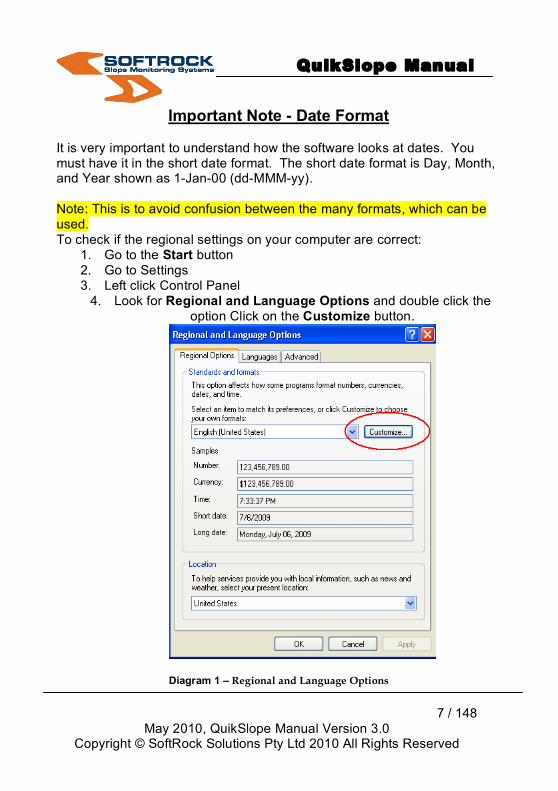
Important Note - Date Format It is very important to understand how the software looks at dates. You must have it in the short date format. The short date format is Day, Month, and Year shown as 1-Jan-00 (dd-MMM-yy). Note: This is to avoid confusion between the many formats, which can be used. To check if the regional settings on your computer are correct:

1. Go to the Start button 2. Go to Settings 3. Left click Control Panel

4. Look for Regional and Language Options and double click the option Click on the Customize button.

Diagram 1 – Regional and Language Options

QuikSlope Manual

8 / 148


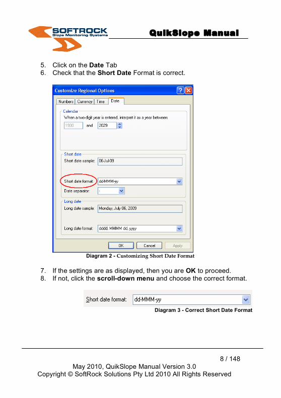
5. Click on the Date Tab 6. Check that the Short Date Format is correct.

Diagram 2 - Customizing Short Date Format

7. If the settings are as displayed, then you are OK to proceed. 8. If not, click the scroll-down menu and choose the correct format.

Diagram 3 - Correct Short Date Format

QuikSlope Manual

9 / 148


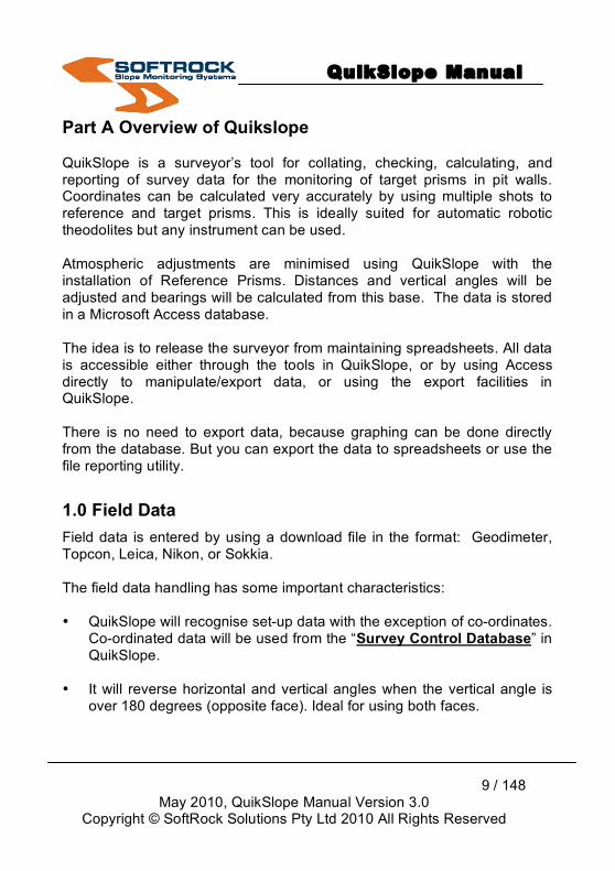
Part A Overview of Quikslope QuikSlope is a surveyor’s tool for collating, checking, calculating, and reporting of survey data for the monitoring of target prisms in pit walls. Coordinates can be calculated very accurately by using multiple shots to reference and target prisms. This is ideally suited for automatic robotic theodolites but any instrument can be used. Atmospheric adjustments are minimised using QuikSlope with the installation of Reference Prisms. Distances and vertical angles will be adjusted and bearings will be calculated from this base. The data is stored in a Microsoft Access database. The idea is to release the surveyor from maintaining spreadsheets. All data is accessible either through the tools in QuikSlope, or by using Access directly to manipulate/export data, or using the export facilities in QuikSlope. There is no need to export data, because graphing can be done directly from the database. But you can export the data to spreadsheets or use the file reporting utility.

1.0 Field Data Field data is entered by using a download file in the format: Geodimeter, Topcon, Leica, Nikon, or Sokkia. The field data handling has some important characteristics: • QuikSlope will recognise set-up data with the exception of co-ordinates.

Co-ordinated data will be used from the “Survey Control Database” in QuikSlope.

• It will reverse horizontal and vertical angles when the vertical angle is over 180 degrees (opposite face). Ideal for using both faces.

QuikSlope Manual

10 / 148


• Ideal for multiple shots to one target. Means and standard deviations will be shown.

• After data is verified, one set of mean observations is sent to the database.

• QuikSlope is ideal for using the full potential of the new breed of

“automatic theodolites”. • Multiple shots to Reference Prisms and Target Prisms result in highly

accurate bearings. • Historical data can be imported using a comma-delimited file (or CSV

Excel file) of the format: ID, Date, Northing, Easting, and Elevation. • If you have been using QuikSlope version 0.9 then you can import the

xyz file for each target and the benchmark data in the .dat file.

1.0.1 Calculations All calculations are handled by “instrument set-up” through the original download file. Each set-up is stamped by a unique ID, the set-up date, and the original file name. The calculations themselves are unique in that they are carried out using the criteria below: • Horizontal angles are based on one of the prisms in the observation

round being a reference prism. In other words one of the target prisms can be used to calculate all the bearings from the mean HA of that target.

• Vertical angles can have an adjustment applied based on the difference between today’s vertical angle and the base (true) vertical angle. This adjustment will be applied by a factor of slope distance. This will help minimise the effect due to atmospherics.

QuikSlope Manual

11 / 148


• Slope distances can be adjusted by the difference between observed distance and the true distance to a known target reference prism. The adjustment will also help minimise the effect due to atmospherics.

• Control coordinates can be stored with a date stamp. Hence all

calculations carried out will be from the coordinates of a station at that point of time. This means that all historic data can be recalculated whenever you wish. Moving control stations are catered for. The true position of target prisms can be achieved by checking the control at regular time intervals using conventional or GPS methods.

1.0.2 Base Reading A set of “base readings” is held on the file. These readings are the “benchmark” data to be used when calculating target movement. Rather than accepting the first reading for a given prism, you may edit the data directly, or use the tool available and calculate a new datum by taking the mean of the first x number of points.

Note: Remember to Recalculate Movements after performing this option.

1.0.3 Reporting Reporting can be done by: • Viewing the data graphically

• Printing a report. • Exporting to a spreadsheet. • Exporting the latest coordinates to a Surpac file. Using Reporting, Create Export File for Spreadsheets from the Toolbar, creates a delimited text file. It contains the following data:

QuikSlope Manual

12 / 148


Target ID, Date, Northing, Easting, RL, Date (numeric), dNorth, dEast, dRL, Adjusted Distance. This file can be used to enter the data into spreadsheets and create graphs. Other reporting functions will be created in the future, including a built in graphing module.

1.0.4 Excel Spreadsheet An automated sequence for loading data (via the above text file qsdata.txt) is available. The sequence:

1. Loads the text file qsdata.txt 2. Checks each line for out-of-bounds data. After all the data is

vetted, some rogue data will still appear. However, a message box will give you the option for deleting it. This data is only deleted from the current spreadsheet you are working on. All data is still on record in an Access database (called qslope.mdb), which is used by QuikSlope.

3. A chart is drawn for each target prism in the area chosen (in

qsdata.txt) and placed on a separate worksheet.

4. If you wish to save the spreadsheet, you will have to use the Save As function in Excel and save it as an ‘FileName.xls’ file and not as a CSV text file which will be the default.

QuikSlope Manual

13 / 148


Part B QuikSlope Main Menu

1.1 Toolbar Below is a layout of the main pull-down menu system (Toolbar).

Diagram 4 - Main Pull-Down Menu – Toolbar

1.1.0 File

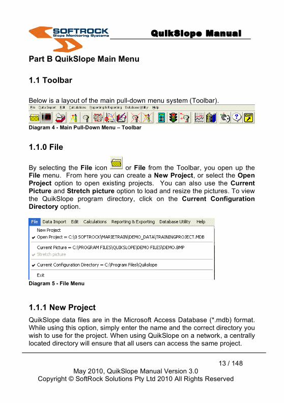
By selecting the File icon or File from the Toolbar, you open up the File menu. From here you can create a New Project, or select the Open Project option to open existing projects. You can also use the Current Picture and Stretch picture option to load and resize the pictures. To view the QuikSlope program directory, click on the Current Configuration Directory option.

Diagram 5 - File Menu

1.1.1 New Project QuikSlope data files are in the Microsoft Access Database (*.mdb) format. While using this option, simply enter the name and the correct directory you wish to use for the project. When using QuikSlope on a network, a centrally located directory will ensure that all users can access the same project.

QuikSlope Manual

14 / 148


1.1.2 Open Project Open an existing project with this option. If a project has been started previously by using the New Project option, then it will be available for use in the Open Project feature. You can use the Windows dialog tools to open local and network files. The current project will be shown on the menu and as the title on the top of the window.

1.1.3 Current Picture The Current Picture option loads a Windows BMP file into the work area. This is handy for aerial photos, plans of the target positions, or close-ups of crack areas. The current picture filename will be shown on the menu item.

1.1.4 Current Configuration Directory

This is a configuration option for QuikSlope. When you operate QuikSlope, it normally reads and writes configuration files in the application directory. On some networks this is undesirable and you can setup QuikSlope to:

• Copy all the configuration files to a new location and set all the pointers to this location.

• Simply just point to the location. When using this feature you will see a warning box saying, “see your systems administrator.” This feature should only be used if absolutely required. Note: When setting up for the first time, enable the Change Dir & Copy Files box.

QuikSlope Manual

15 / 148


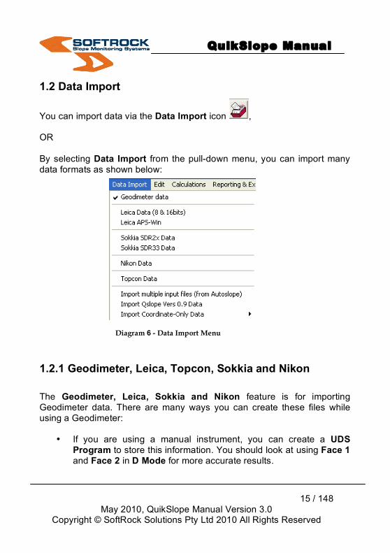
1.2 Data Import

You can import data via the Data Import icon , OR By selecting Data Import from the pull-down menu, you can import many data formats as shown below:

1.2.1 Geodimeter, Leica, Topcon, Sokkia and Nikon The Geodimeter, Leica, Sokkia and Nikon feature is for importing Geodimeter data. There are many ways you can create these files while using a Geodimeter:

• If you are using a manual instrument, you can create a UDS Program to store this information. You should look at using Face 1 and Face 2 in D Mode for more accurate results.

Diagram 6 - Data Import Menu

QuikSlope Manual

16 / 148


• If you are using a servo driven instrument, then you might look at utilising Program 23 to drive to each target point. See “Geoimeter servo driven procedures”.

• If you are using a Geodimeter ATS, or Leica TCA1100 which are

automated lock-on survey robots, you will need nothing else but QuikSlope.

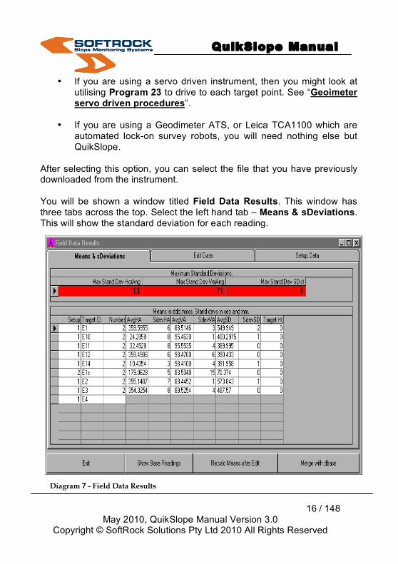
After selecting this option, you can select the file that you have previously downloaded from the instrument. You will be shown a window titled Field Data Results. This window has three tabs across the top. Select the left hand tab – Means & sDeviations. This will show the standard deviation for each reading. Diagram 7 - Field Data Results

QuikSlope Manual

17 / 148


Note: The maximums are shown in the red line at the top. (Diagram 7) The results will be inaccurate if the data is aligned with an incorrect Target ID. Take note of what Target IDs are having a problem and select the centre tab Edit Data. All the data in the Edit Data window are changeable. The data is sorted by Target ID, so you can easily find all the data to do with a particular Target Prism. Complete lines of data can be erased by selecting any cell on that line, highlighting that line by hitting the left hand tab button and using the delete key on the keyboard. After editing the data, use the Recalc Means after Edit button and check the standard deviations again. Re-edit until the standard deviations are acceptable. Note: Remember you need at least two readings to get a true standard deviation. To help with editing you can view the previous data at the bottom of the window. Accept the data and use the Merge with dbase button.

1.2.2 Import Qslope Vers 0.9 Data Use this function to import data from the earlier DOS version 0.9. In this version each target data is kept in a separate ASCII file called *.xyz. Each of these files needs to be imported. The benchmark data, which is in a file called qsdata.dat, can also be imported.

1.2.3 Import Coordinate only Data This option is for loading historical data from other sources. Simply make a comma-delimited file in the following formats:

QuikSlope Manual

18 / 148


• Target ID, Date, Time, Northing, Easting, Elevation

• Target ID, Date, Time, Slope Distance, Northing, Easting, Elevation

• Target ID, Easting, Northing, Elevation, Text • Target ID, Northing, Easting, Elevation, Dataset number.

If your data is in a spreadsheet, then make up the columns as above, and export to a file. If using Excel then save as a CSV file. The last dataset is when you wish to import edited data. This data is typical of QuikSlope data that has been exported using the export spreadsheet function i.e. it exports the dataset number. The xyz data is then edited. When editing, ensure the dataset number is still attached to the original data. This CSV file is created from the edited data. The dataset number will ensure that the edited data is written over the existing dataset. Note: Be careful using this last function. It will change your existing data.

1.2.4 Data Structure QuikSlope stores all data in a MS Access database. The database format is Access97 and this should not be updated to a later version of Access. You can use Access2000 to edit data, but do not upgrade the file to Access2000; otherwise QuikSlope will be unable to read the database. This database will be upgraded by later versions of QuikSlope. The measurement data is held in two main tables.

a. Setup Data. This contains one record for any one setup that has the following fields:

QuikSlope Manual

19 / 148


1. Setup Number - This is a unique number that connects the measurement data to the setup data.

2. File ID - Name of import file.

3. Instrument station

4. HI - Height Instrument. 5. REF HA Target - The REF prism used for adjustments.

6. Date

7. Time

8. Ppm - The ppm setting from the instrument. This is a good

guide to the quality of measured distances.

9. Calc VA correction - The VA adjustment factor (per 1000M)

10. Calc SD correction - The Sd adjustment factor (per 1000M)

b. Data. There can be one or hundreds of data records that can refer back to the Setup table. The data table holds all the measured field data and calculated data. The fields are:

1. Setup number - The setup number in the setup table. 2. Target ID - Prism name.

3. Target Ht - Normally zero.

4. HA, VA and SD - Mean field measured data. This data is the

average of multiple readings.

5. sDevHa, sDevVa, sDevSd - The standard deviations of field data.

QuikSlope Manual

20 / 148


6. Number Shots - The number of shots taken from which the mean is calculated.

7. HaAdjusted, VaAdjusted, SdAdjusted - The adjusted HA, VA

and SD. This adjustment refers to the REF adjustments.

8. North, East, RL - The calculated YXZ coordinates.

9. DHA, dVA, dSD - The difference in field data from the benchmarks.

10. DN, dE, dRL - The delta movements of YXZ from the

benchmark N, E, and RL

11. 90 day velocity - This contains the calculated velocity. It is not really a 90-day velocity but is the latest movement expressed in mm/day but multiplied by 90. So if we divide the value by 90 we will get the latest velocity expressed in mm per day.

Velocity is calculated by taking the latest slope distance and subtracting it from the Sd of the previous reading. We also take the date and time of these readings into account, and extrapolate it to 1 x 24 hour day.

12. Benchmark - This contains the benchmark or base data from

which all movements are calculated. It is also how area names are allotted. There should be only one record per prism in this table.

13. Control - Survey control data (including REF prisms) is kept

here.

14. Control Names - Table connects via the Control table.

15. Crack Names - Crack monitoring locations.

16. Cracks - This contains crack readings.

QuikSlope Manual

21 / 148


17. Events - This table contains a memo field for event recording.

18. Pit area - This field contains max and mins for graphic location of area view.

19. Pit crests - Contains XY of crest lines.

20. Pit Toes - Contains XY of toe lines for graphic reproduction.

21. Pit Max/Min - Contains the graphic maximum and minimum

XY for whole pit.

22. Rainfall - This table has date and rain gauge reading.

23. Seismic - This table contains Date/Time/Richter reading/Distance. This contains seismic data of seismic events.

Editing data directly in Access is not recommended as it could affect the operation of QuikSlope. Note: It is recommended to have a backup copy of the database at all times.

QuikSlope Manual

22 / 148


1.3 Edit By selecting the Edit pull-down menu the user has the option of carrying out edit functions.

Diagram 8 - Edit pull-down menu

1.3.1 Edit Setup Data All data sets in the database have a corresponding setup number, date, Instrument Station, Height Instrument, etc. This is kept in a table, which is accessible by selecting Edit Setup Data from - Edit pull-down menu or

clicking toolbar icon .

QuikSlope Manual

23 / 148


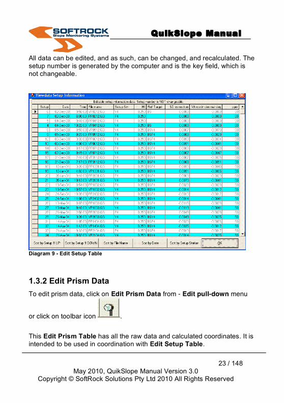
All data can be edited, and as such, can be changed, and recalculated. The setup number is generated by the computer and is the key field, which is not changeable.

Diagram 9 - Edit Setup Table

1.3.2 Edit Prism Data To edit prism data, click on Edit Prism Data from - Edit pull-down menu

or click on toolbar icon .

This Edit Prism Table has all the raw data and calculated coordinates. It is intended to be used in coordination with Edit Setup Table.

QuikSlope Manual

24 / 148


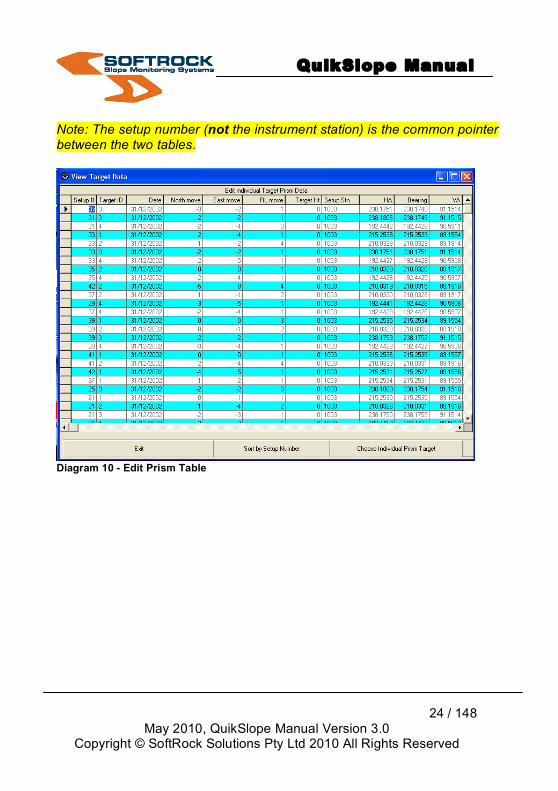
Note: The setup number (not the instrument station) is the common pointer between the two tables.

Diagram 10 - Edit Prism Table

QuikSlope Manual

25 / 148


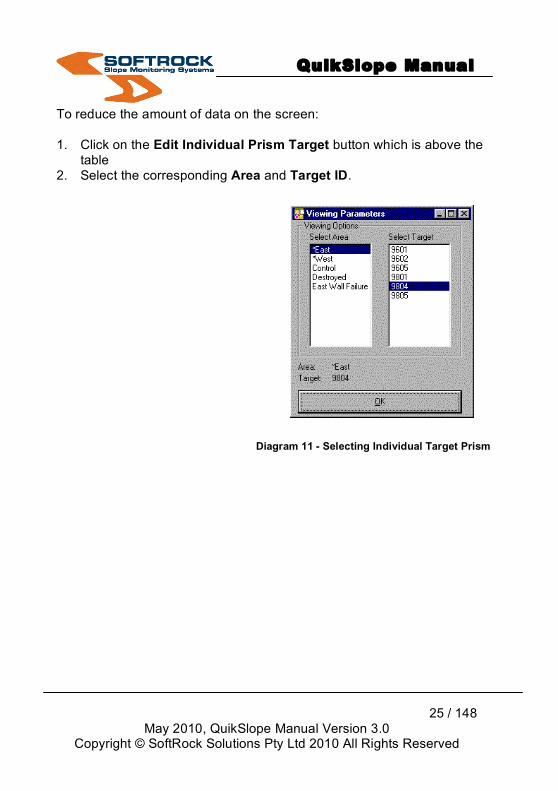
To reduce the amount of data on the screen: 1. Click on the Edit Individual Prism Target button which is above the

table 2. Select the corresponding Area and Target ID.

Diagram 11 - Selecting Individual Target Prism

QuikSlope Manual

26 / 148


1.3.3 Delete Data

There are two ways of deleting data. 1. Delete all data in the database for a particular Prism 2. Delete all data in the database for a particular setup.

1.3.3.1 Delete Prism To delete a prism, click on Delete Prism sub-menu (under Delete Data

from - Edit pull-down menu) or by clicking the toolbar button ,

Note: Deleting a prism will erase all entries of a particular Target ID.

If you have damaged or destroyed targets that you no longer use, it may be better to utilise the Area Name database, and shift all these targets into an area named Destroyed or Recycled.

QuikSlope Manual

27 / 148


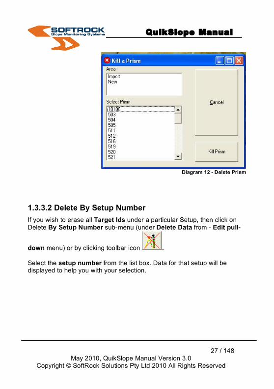
Diagram 12 - Delete Prism

1.3.3.2 Delete By Setup Number If you wish to erase all Target Ids under a particular Setup, then click on Delete By Setup Number sub-menu (under Delete Data from - Edit pull-

down menu) or by clicking toolbar icon . Select the setup number from the list box. Data for that setup will be displayed to help you with your selection.

QuikSlope Manual

28 / 148


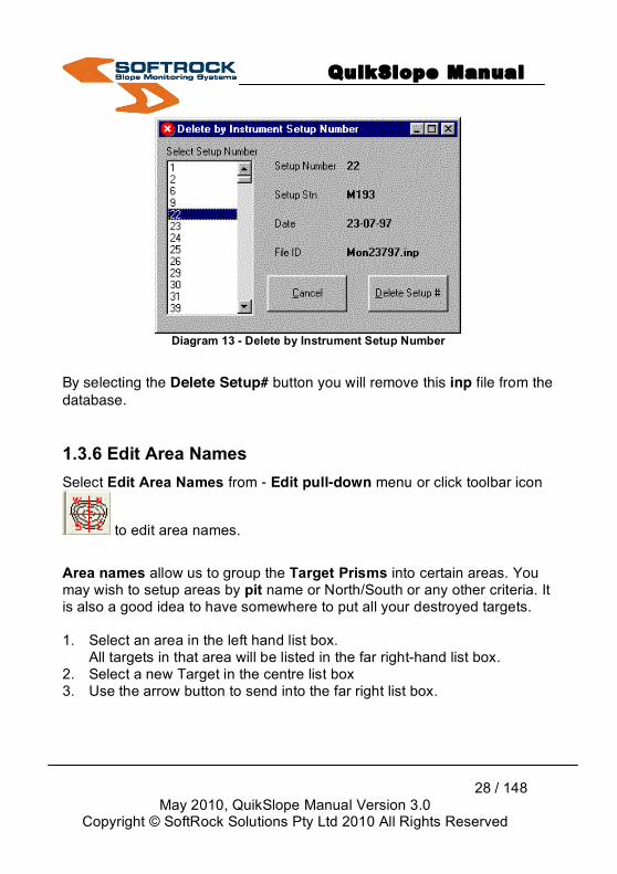
Diagram 13 - Delete by Instrument Setup Number

By selecting the Delete Setup# button you will remove this inp file from the database.

1.3.6 Edit Area Names Select Edit Area Names from - Edit pull-down menu or click toolbar icon

to edit area names.

Area names allow us to group the Target Prisms into certain areas. You may wish to setup areas by pit name or North/South or any other criteria. It is also a good idea to have somewhere to put all your destroyed targets. 1. Select an area in the left hand list box.

All targets in that area will be listed in the far right-hand list box. 2. Select a new Target in the centre list box 3. Use the arrow button to send into the far right list box.

QuikSlope Manual

29 / 148


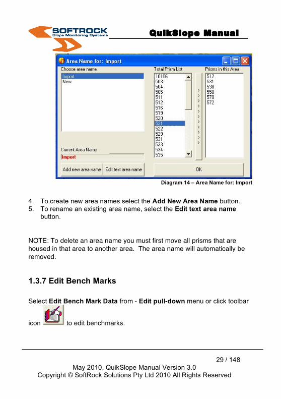
Diagram 14 – Area Name for: Import

4. To create new area names select the Add New Area Name button. 5. To rename an existing area name, select the Edit text area name

button.

NOTE: To delete an area name you must first move all prisms that are housed in that area to another area. The area name will automatically be removed.

1.3.7 Edit Bench Marks Select Edit Bench Mark Data from - Edit pull-down menu or click toolbar

icon to edit benchmarks.

QuikSlope Manual

30 / 148


The Benchmark data refers to the original data set. This data can be changed for various reasons:

• To reflect changes to raw data when using a different instrument station.

• Due to bad measurements in the original dataset • Using the mean the first 10 (or whatever number is required)

readings to achieve a more accurate benchmark

Diagram 15 - Editing Bench Marks

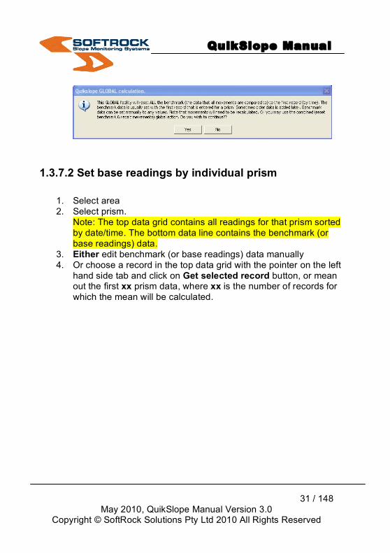
1.3.7.1 Set Base Reading globally We can set benchmark data globally or individually. To set it globally by area name, it can only be done when the benchmark window first appears as shown above:

1. Choose the area first. 2. Click on the button Set all prisms in the area to initial reading. 3. By clicking on the Globally reset all benchmark data to first

record of complete database, you can reset the benchmark by g yes on the confirmation box.

QuikSlope Manual

31 / 148


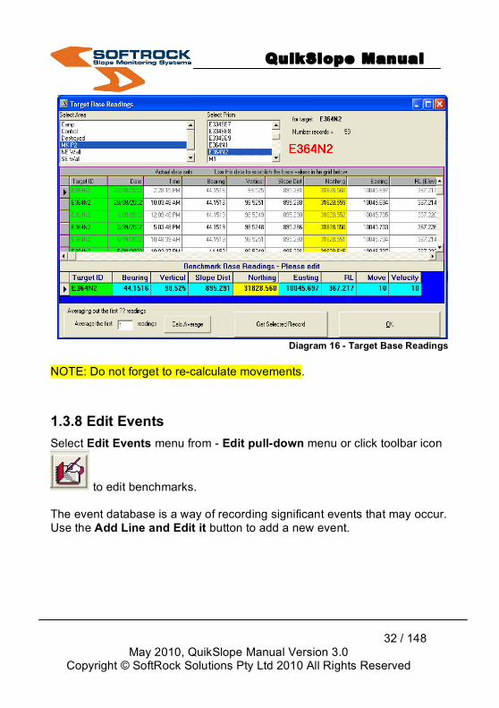
1.3.7.2 Set base readings by individual prism

1. Select area 2. Select prism.

Note: The top data grid contains all readings for that prism sorted by date/time. The bottom data line contains the benchmark (or base readings) data.

3. Either edit benchmark (or base readings) data manually 4. Or choose a record in the top data grid with the pointer on the left

hand side tab and click on Get selected record button, or mean out the first xx prism data, where xx is the number of records for which the mean will be calculated.

QuikSlope Manual

32 / 148


Diagram 16 - Target Base Readings

NOTE: Do not forget to re-calculate movements.

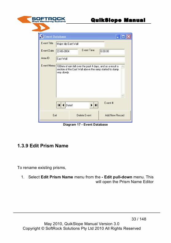
1.3.8 Edit Events Select Edit Events menu from - Edit pull-down menu or click toolbar icon

to edit benchmarks. The event database is a way of recording significant events that may occur. Use the Add Line and Edit it button to add a new event.

QuikSlope Manual

33 / 148


Diagram 17 - Event Database

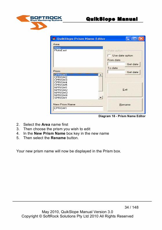
1.3.9 Edit Prism Name To rename existing prisms,

1. Select Edit Prism Name menu from the - Edit pull-down menu. This will open the Prism Name Editor

QuikSlope Manual

34 / 148


Diagram 18 - Prism Name Editor

2. Select the Area name first 3. Then choose the prism you wish to edit 4. In the New Prism Name box key in the new name 5. Then select the Rename button. Your new prism name will now be displayed in the Prism box.

QuikSlope Manual

35 / 148


Diagram 19 - List of Prism Names

1.3.10 Rainfall To keep a record of rainfall in your area, select Rainfall from - Edit pull-down menu. Simply fill in with the date and gauge reading data. You can also select the Import a file function, which will import a delimited ASCII file. Each line should contain the following: (date), (rain gauge reading). This can be a csv file from excel. To view this data, go to the graphing function and select rainfall in graph type.

Diagram 20 - Rainfall

QuikSlope Manual

36 / 148


1.3.11 Crack Monitors To keep records of cracks around the working pit, select Crack Monitors from - Edit pull-down menu. This will in open 2 sub-menus as shown below:

Diagram 21 - Crack monitors menus

Recording cracks records is a 2-step process: 1. Step 1 Select the Crack Monitor name and location menu. Fill in the table with the crack name and co-ordinates. You can also import in the form of a delimited ASCII file.

Diagram 22 - Crack Monitor Master List

QuikSlope Manual

37 / 148


2. Step 2

i. Select Crack monitor readings menu.

Diagram 23 - Crack Monitor Readings

i. Then add your readings to a table for the crack names.

ii. Fill in the crack name, date, time and reading (in mm). Again you can import this information as an ASCII file in the format of: (crack name) (northing) (easting) (elevation) and (description).

• The Resort button allows you to sort the cracks in ascending order.

QuikSlope Manual

38 / 148


• You can also select individual crack monitor readings using the Select Individual button. By simply selecting the Add a new Crack Monitor button you can add a new crack monitor from here to your master list.

NOTE: don’t forget to fill in the readings in your Crack Monitor readings table for the new crack name if you are using this button.

• If you require to delete any data from either the Crack Monitor Name

and Location or Crack Monitor Readings table, highlight the row using your mouse. Then select the delete button from the keyboard and choose OK to delete the row.

• To graph these readings simply go to the graphing facility and choose

crack movement for your graph type and then select the crack name. You can also plot the location of these crack monitors under the View Plan Plot menu.

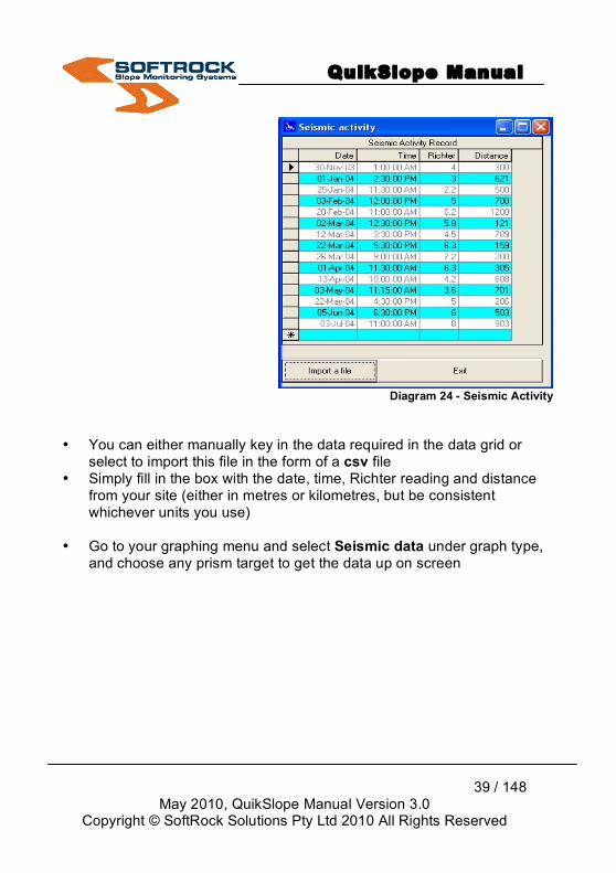
1.3.12 Seismic Activity Click on Seismic Activity from - Edit pull-down menu to add seismic information in the form of date, Richter value and distance where the tremor occurred from your location.

QuikSlope Manual

39 / 148


Diagram 24 - Seismic Activity

• You can either manually key in the data required in the data grid or

select to import this file in the form of a csv file • Simply fill in the box with the date, time, Richter reading and distance

from your site (either in metres or kilometres, but be consistent whichever units you use)

• Go to your graphing menu and select Seismic data under graph type,

and choose any prism target to get the data up on screen

QuikSlope Manual

40 / 148


1.4 Calculations

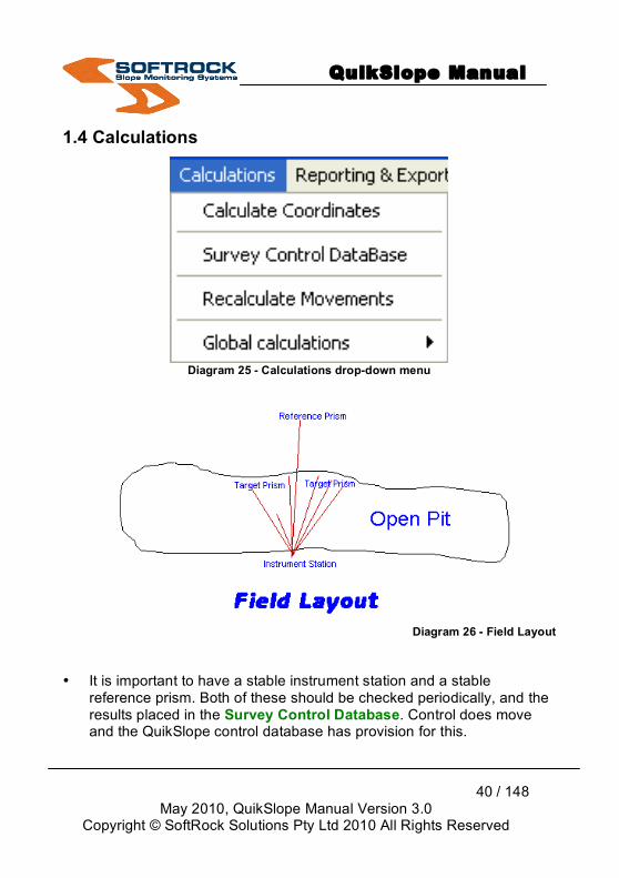
Diagram 25 - Calculations drop-down menu

Diagram 26 - Field Layout

• It is important to have a stable instrument station and a stable

reference prism. Both of these should be checked periodically, and the results placed in the Survey Control Database. Control does move and the QuikSlope control database has provision for this.

QuikSlope Manual

41 / 148


• The reference prism should be placed so that when you measure to it, it is measuring through the same column of air as the target prisms. Then you can take advantage of the full adjusting features of QuikSlope.

• Horizontal angles are calculated from the reference prism, which will be one of the prisms in the observation round. So all bearings will be based on multiple angles taken to the reference prism. NOTE: This takes full advantage of robotic instruments as no calculations are based on optical pointing.

• Vertical angles will have an adjustment applied based on the difference

to the reference prism. This adjustment will be applied by a factor of slope distance. This will help minimise the affect due to atmospherics.

• Slope distances will also be adjusted by the difference to the reference

prism. The adjustment will be applied by a factor of slope distance. This will also help minimise the affect due to atmospherics.

• Control coordinates can be stored with a date stamp. Hence all

calculations carried out will be from the coordinates of a station at that point in time. This means that all historic data can be recalculated at any time. Moving control stations can still be utilised. By checking the control at regular time intervals by conventional or GPS methods, the true position of target prisms can be achieved.

1.4.1 Calculate Co-ordinates

To calculate co-ordinates, click on Calculate Co-ordinates from the -

Calculations drop-down menu or click on toolbar icon .

QuikSlope Manual

42 / 148


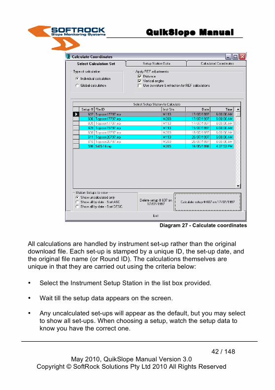
Diagram 27 - Calculate coordinates

All calculations are handled by instrument set-up rather than the original download file. Each set-up is stamped by a unique ID, the set-up date, and the original file name (or Round ID). The calculations themselves are unique in that they are carried out using the criteria below: • Select the Instrument Setup Station in the list box provided.

• Wait till the setup data appears on the screen.

• Any uncalculated set-ups will appear as the default, but you may select

to show all set-ups. When choosing a setup, watch the setup data to know you have the correct one.

QuikSlope Manual

43 / 148


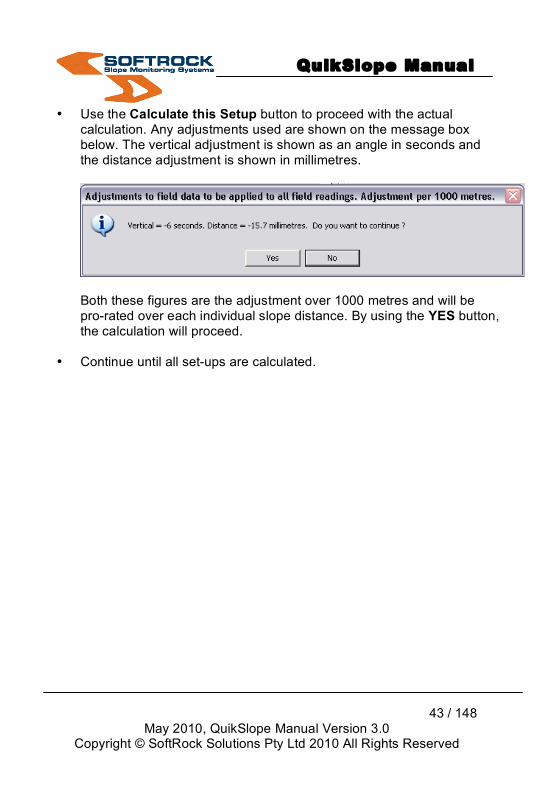
• Use the Calculate this Setup button to proceed with the actual calculation. Any adjustments used are shown on the message box below. The vertical adjustment is shown as an angle in seconds and the distance adjustment is shown in millimetres.

Both these figures are the adjustment over 1000 metres and will be pro-rated over each individual slope distance. By using the YES button, the calculation will proceed.

• Continue until all set-ups are calculated.

QuikSlope Manual

44 / 148


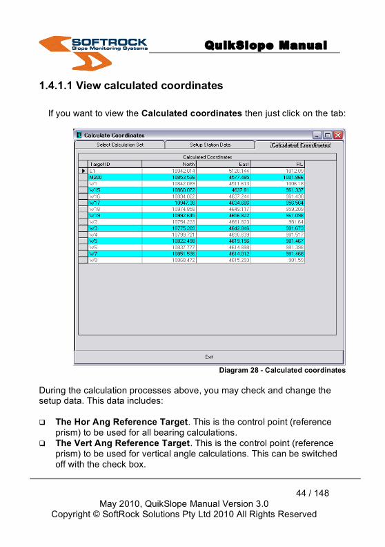
1.4.1.1 View calculated coordinates

If you want to view the Calculated coordinates then just click on the tab:

Diagram 28 - Calculated coordinates

During the calculation processes above, you may check and change the setup data. This data includes: The Hor Ang Reference Target. This is the control point (reference

prism) to be used for all bearing calculations. The Vert Ang Reference Target. This is the control point (reference

prism) to be used for vertical angle calculations. This can be switched off with the check box.

QuikSlope Manual

45 / 148


The Distance Reference Target. This is the control point (reference prism) to be used for all distance calculations. It is simply used to apply a scale factor. This can be switched off with the check box.

1.4.1.2 Calculate Adjustment Factors Use the Calculate Adjustment Factors button (under Setup Station Data tab) to check the adjustment factors at any time. The Vertical adjustment will be shown as a vertical angle (ddd.mmss) per 1000 metres. So for a distance of 500 metres only half of this angular correction will be applied. The slope distance correction is shown as a distance per 1000 metres. The horizontal correction refers to the difference to bearings. NOTE: The above is not optional.

Diagram 29 - Setup Station Data

QuikSlope Manual

46 / 148


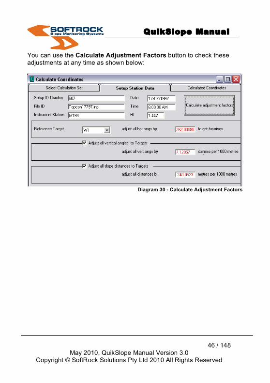
You can use the Calculate Adjustment Factors button to check these adjustments at any time as shown below:

Diagram 30 - Calculate Adjustment Factors

QuikSlope Manual

47 / 148


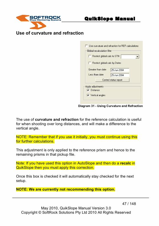
Use of curvature and refraction

Diagram 31 - Using Curvature and Refraction

The use of curvature and refraction for the reference calculation is useful for when shooting over long distances, and will make a difference to the vertical angle. NOTE: Remember that if you use it initially, you must continue using this for further calculations. This adjustment is only applied to the reference prism and hence to the remaining prisms in that pickup file. Note: If you have used this option in AutoSlope and then do a recalc in QuikSlope then you must apply this correction. Once this box is checked it will automatically stay checked for the next setup. NOTE: We are currently not recommending this option.

QuikSlope Manual

48 / 148


You are now ready to apply the graphing, reporting and exporting functions for your prism information.

1.4.2 Survey Control Database

To view and edit control data, click on Survey Control Database from the -

Calculations drop-down menu or click on toolbar icon . Control data includes instrument stations and reference targets. Each control point can have multiple entries which is meant to cater for basically two things: 1. Moving coordinates. 2. Change in reference point. The control should be checked periodically so that updated xyz values can be added. That is why the date is an important part of the control database. Calculation errors can occur if the date of the setup data precedes the date of the earliest control listing. The first control data date has to precede the initial setup.

QuikSlope Manual

49 / 148


Diagram 32 - Control Coordinate Data Form

1.4.2.1 Add and editing control data 1. Select a Control Point in the list box or use Add Control Point button

(for new control) and select it. 2. Use the Add New Date Line to add a new line of data. 3. A new data line will be added using today’s date. You can edit the data. 4. Ref HA Target, Ref VA Target, and the Ref SD Target refer to the

reference prism. It is possible to have a different reference for calculating bearings (HA), adjusting vertical angles (VA) and adjusting distances (SD). Usually you will use the same reference for each.

5. Either select an existing control point from the listing, or use the Add

control point button. You will firstly be prompted to select a Control Point as shown in the dialog box below.

Note 1: You need to include all instrument stations and reference targets (prisms).

QuikSlope Manual

50 / 148


Note 2: You can have multiple listings of the one control point.

6. Use the Delete button to delete control points. If you wish to delete a record, simply select any cell on that row, and select the button on the left so that the complete row is highlighted, and then use the delete key on the keyboard.

7. You can also import control data in CSV format, simply select the

Import a CSV file button. Follow the prompts, and the data will be placed in the QuikSlope Database.

The concept is to track the position of control points by date, and retain this historical data so that future recalculations can be done at any time. Note 3: Ensure that your earliest date is earlier (or the same) than the date of the first set of readings.

1.4.2.2 Multiple References • To align Quikslope with Autoslope, we need to be able to do

recalculations when multiple references are in use. Autoslope can use multiple references when there is a likelihood of an inability to see a reference all the time, so we can fallback to another two references.

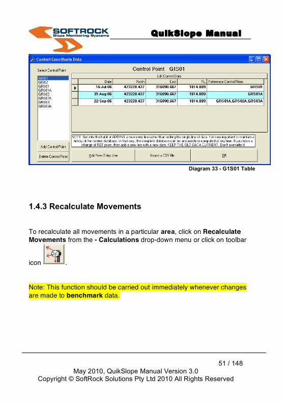
• To recalculate data that has been measured using multiple REFs, the control (all the REF prisms) are entered individually as normal, but on the instrument control (see - G1S01 Table below), instead of entering a single REF control station in the last column, we can enter multiple ones by delineating with commas. So on the bottom line we can use references GRS01A or GRS02A or GRS03A. So when we perform a recalculation in Quikslope, the first available REF in this order will be used as a bearing reference. Remember to turn OFF the adjustments.

QuikSlope Manual

51 / 148


Diagram 33 - G1S01 Table

1.4.3 Recalculate Movements

To recalculate all movements in a particular area, click on Recalculate Movements from the - Calculations drop-down menu or click on toolbar

icon .

Note: This function should be carried out immediately whenever changes are made to benchmark data.

QuikSlope Manual

52 / 148


Diagram 34 - Recalculate Movements

• If there are changes to control or to your benchmark readings then you can recalculate the delta movements for the specific areas. This option will remove obvious jumps in distance from the previous reading. Use the default jump distance or set your own. Note: If you change benchmark readings do a recalculate delta movement

• When you import old readings you can get flat-lining data e.g. The

graph appears flat and there are no delta differences calculated. • If you change your benchmark data for all (or some) areas then the

global function is useful.

QuikSlope Manual

53 / 148


• If the control is changed for the prisms being monitored you have the facility to use the global function to recalculate the movements. (This function will cut down the re-processing time).

1.4.4 Global Calculations To perform global calculations, click on Global Calculations from the - Calculations drop-down menu. This consists of a number of options that have been designed to save you time when performing major changes to your database. Note: If your database is large some of these calculations can take a bit of time to perform. It is also a good idea prior to performing these changes to copy your database to another directory. There is no undo button to reverse these calculations.

Diagram 35 - Global Calculation Options

1.4.4.1 Recalculate All Coordinates in Database This option is designed to recalculate all the co-ordinates for your Prism data. Your control and reference prism data must be maintained correctly for this option.

QuikSlope Manual

54 / 148


QuikSlope uses all changes in station and reference control to recalculate the preceding set-ups. If the either of this control data has changed for various reasons since the initial set-ups, then these changes will also be reflected in the co-ordinates for the observed prisms.

Diagram 36 - Example of temp-qs.txt

QuikSlope will create a report temp-qs.txt with all the distance and vertical adjustment factors applied.

1.4.4.2 Reset all Benchmark Data to the First Record This global facility will reset all the benchmark data to the first record by date. The benchmark data is usually set with the first record that is entered

QuikSlope Manual

55 / 148


for a prism. Sometimes older data is added later. Benchmark data can be manually set to any value. Note: Movements will need to be recalculated. You can use the combined (reset benchmark and recalculate movements of all prisms) global action. This action will change the delta movements for a prism.

1.4.4.3 Recalculate Movements for all Prisms This option will recalculate all the delta movements for all data in your database. It may be a good idea to reset the benchmark data first. It will ask you to enter a jump distance for the adjusted distance option in the graphing mode. Normally a minimum distance of 0.5 is the default. This jump distance is normally used when a site changes control stations to monitor the same prisms. In order to be able to graph using the distance function, we are required to enter a jump distance, which will eliminate this change in distance observation to the prisms. The co-ordinates of the prisms will still be correct.

1.4.4.4 Reset all Benchmarks and Calculate Movements This option will reset all the benchmarks to the first observation and recalculate the deltas of the entire database. You also have the option here to enter a jump distance if you wish.

QuikSlope Manual

56 / 148


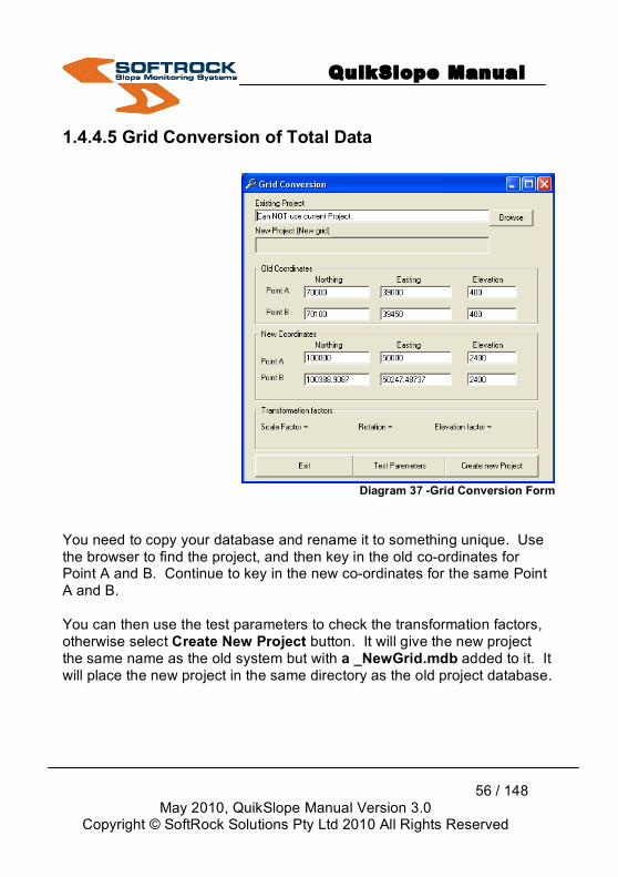
1.4.4.5 Grid Conversion of Total Data

Diagram 37 -Grid Conversion Form

You need to copy your database and rename it to something unique. Use the browser to find the project, and then key in the old co-ordinates for Point A and B. Continue to key in the new co-ordinates for the same Point A and B. You can then use the test parameters to check the transformation factors, otherwise select Create New Project button. It will give the new project the same name as the old system but with a _NewGrid.mdb added to it. It will place the new project in the same directory as the old project database.

QuikSlope Manual

57 / 148


1.4.4.6 Set Zero Adj Distance to Equal Unadj Distance When using the second import function Import Id, Date, Time, S-Dist, N, E, RL, you might get some distances coming out as zero, therefore disallowing you to calculate data. This function will reset any zero distances to equal unadjusted distances. QuikSlope will reset the benchmark data and recalculate it. The default distance of 0.5m is still used, unless you decide to change this.

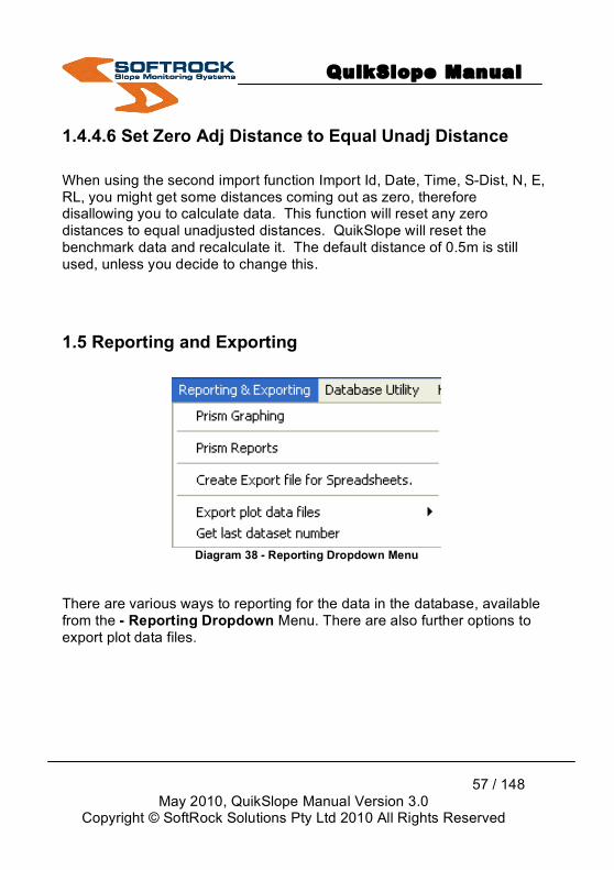
1.5 Reporting and Exporting

Diagram 38 - Reporting Dropdown Menu

There are various ways to reporting for the data in the database, available from the - Reporting Dropdown Menu. There are also further options to export plot data files.

QuikSlope Manual

58 / 148


1.5.1 Prism Graphing To select the prism graphing tool, click on Prism Graphing from the -

Reporting Dropdown Menu or click on toolbar icon . The graph tool is based on the “Graph Control” version 5.80 by Pinnacle Publishing. It is a powerful tool that is being constantly updated. QuikSlope will incorporate these releases from time to time.

1.5.1.1 24 Hour Report When you first open the Graphing window a 24-hour report is displayed, detailing the prism and prism groups, which have been read in the past 24 hours, together with any movement, which falls outside the specified thresholds. It shows any alarms that have been activated and on which prisms. It shows all the latest movements for all prisms, in a file tree format.

QuikSlope Manual

59 / 148


Diagram 39 - 24-hour report

1.5.1.2 Graph Views

Diagram 40 - Various graph views options

We have tried to create a tool that encapsulates all your graphing and plan views from the one window. There are six viewing areas –

1. a plan view for creating plots, 2. a location view

QuikSlope Manual

60 / 148


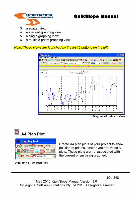
3. a scatter view 4. a stacked graphing view 5. a single graphing view 6. a multiple prism graphing view.

Note: These views are launched by the first 6 buttons on the left.

Diagram 41 - Graph View

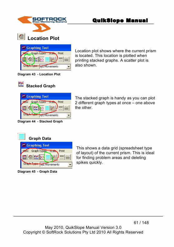
A4 Plan Plot

Create A4 plan plots of your project to show position of prisms, scatter vectors, velocity plots. These plots are not associated with the current prism being graphed.

Diagram 42 - A4 Plan Plot

QuikSlope Manual

61 / 148


Location Plot

Location plot shows where the current prism is located. This location is plotted when printing stacked graphs. A scatter plot is also shown.

Diagram 43 - Location Plot

Stacked Graph

The stacked graph is handy as you can plot 2 different graph types at once – one above the other.

Diagram 44 - Stacked Graph

Graph Data This shows a data grid (spreadsheet type of layout) of the current prism. This is ideal for finding problem areas and deleting spikes quickly.

Diagram 45 - Graph Data

QuikSlope Manual

62 / 148


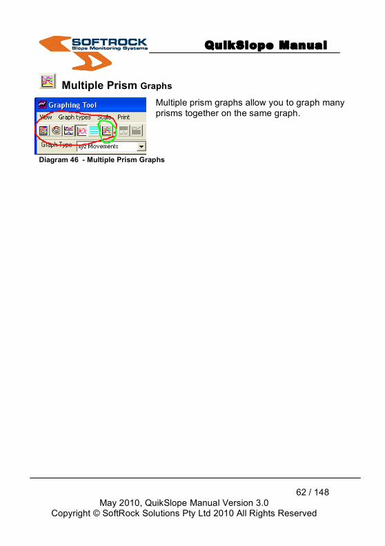
Multiple Prism Graphs

Multiple prism graphs allow you to graph many prisms together on the same graph.

Diagram 46 - Multiple Prism Graphs

QuikSlope Manual

63 / 148


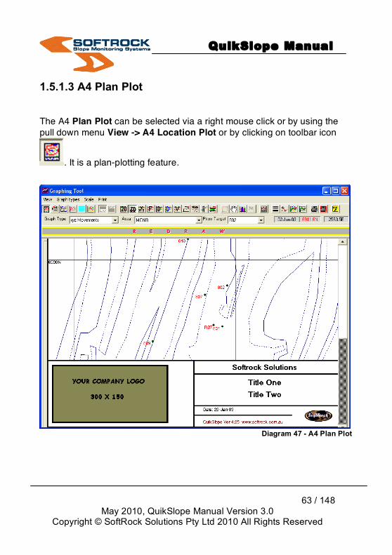
1.5.1.3 A4 Plan Plot

The A4 Plan Plot can be selected via a right mouse click or by using the pull down menu View -> A4 Location Plot or by clicking on toolbar icon

. It is a plan-plotting feature.

Diagram 47 - A4 Plan Plot

QuikSlope Manual

64 / 148


1.5.1.4 View Location Plot

This will redraw all the line work in the plan. It is the same as clicking on the redraw button.

1.5.1.5 Zoom in Window

You can use the menu item Zoom in window or the toolbar button to zoom in using bottom left and top right window positions.

1.5.1.6 Zoom In Zoom in on the current position by 150% of the view

1.5.1.7 Zoom Out

Zoom out by 50% of current view.

1.5.1.8 Draw All Zoom to extents of data

1.5.1.9 Pan

QuikSlope Manual

65 / 148


• Select the Pan button .

• Hold down the left mouse button and drag to desired position. The cursor will change shape during the drag process. Note: The graphic will not drag with the cursor until released.

• This function is only to be used for plan view of pits, and not in graph mode.

1.5.1.10 Load Plan This is how the project open cut plan (or other plans) is loaded into the database. It is done in 2 parts: 1. Load the crests lines (solid lines) 2. Load the toe lines (dash lines) The type of both files above is a Surpac string file. The structure of a Surpac string file is:

1. 2 header lines 2. string #, North, East, Elev, Description 3. 0,0,0,0, (a zero line is at the end of each string.) 4. 0,0,0,0, END (This is the footer line)

1.5.1.11 Draw Current Area View An area view can be saved under View scatter location plan. You may wish to save a view of the west side of the pit to get a closer view of all the prisms in that area. This view is also used in the printout of the stacked graphs.

QuikSlope Manual

66 / 148


1.5.1.12 Draw Area Prisms By checking this option all the prisms in the current area will be shown on the plot. The current area can also be All Prisms.

1.5.1.13 Draw Velocity Plot Only the prisms that exceed certain velocities are shown by colour depending on speed. Total movement is shown by size of the prism circle. This option is under construction at Feb 03.

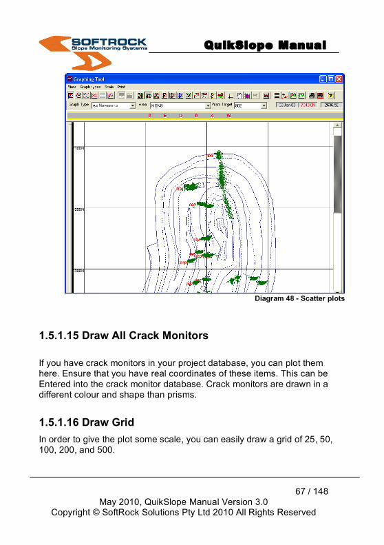
1.5.1.14 Draw Scatters Scatter plots are handy in showing if the prisms are moving in one particular direction and show what that direction is. The scatter is shown by exaggerating the scale around each prism. A slider will appear on the plot, and this is used to select the degree of scale around each prism. The larger the scale factor, the more spread out the scatter plot becomes.

QuikSlope Manual

67 / 148


Diagram 48 - Scatter plots

1.5.1.15 Draw All Crack Monitors If you have crack monitors in your project database, you can plot them here. Ensure that you have real coordinates of these items. This can be Entered into the crack monitor database. Crack monitors are drawn in a different colour and shape than prisms.

1.5.1.16 Draw Grid In order to give the plot some scale, you can easily draw a grid of 25, 50, 100, 200, and 500.

QuikSlope Manual

68 / 148


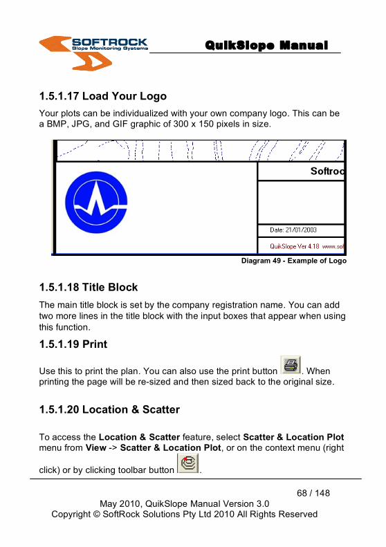
1.5.1.17 Load Your Logo Your plots can be individualized with your own company logo. This can be a BMP, JPG, and GIF graphic of 300 x 150 pixels in size.

Diagram 49 - Example of Logo

1.5.1.18 Title Block The main title block is set by the company registration name. You can add two more lines in the title block with the input boxes that appear when using this function.

1.5.1.19 Print

Use this to print the plan. You can also use the print button . When printing the page will be re-sized and then sized back to the original size.

1.5.1.20 Location & Scatter To access the Location & Scatter feature, select Scatter & Location Plot menu from View -> Scatter & Location Plot, or on the context menu (right

click) or by clicking toolbar button .

QuikSlope Manual

69 / 148


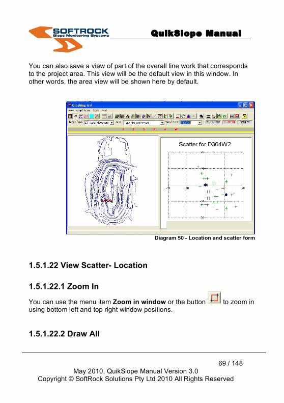
You can also save a view of part of the overall line work that corresponds to the project area. This view will be the default view in this window. In other words, the area view will be shown here by default.

Diagram 50 - Location and scatter form

1.5.1.22 View Scatter- Location 1.5.1.22.1 Zoom In

You can use the menu item Zoom in window or the button to zoom in using bottom left and top right window positions. 1.5.1.22.2 Draw All

QuikSlope Manual

70 / 148


This will redraw all the line work in the plan. It is the same as clicking on the redraw button.

1.5.1.22.3 Redraw Current Area The saved area view for the current area will be recalled. If there is no area view, then a redraw to extents of data will be applied. 1.5.1.22.4 Pan Pan data by holding down on left mouse button and dragging to desired position. The cursor will change shape during the drag process. Note that the graphic will NOT drag with the cursor until released. You can also use the pan button. 1.5.1.22.5 Load New Crest See Section 1.5.1.10 1.5.1.22.6 Load New Toes See Section 1.5.1.10 1.5.1.22.7 Save Current View You can save a view that corresponds to the current area. By zooming and panning you can set your area view then use this option to save it. When printing using stacked graphs, this view will be used by default.

QuikSlope Manual

71 / 148


1.5.1.22.8 Print This feature is not implemented. Use the view stacked graphs and print using print button.

1.5.1.23 Stacked Graphs View

Click toolbar button to select Stacked Graphs View. allows you to plot two different views at once, one over the other. All the time graphs are true time graphs, in that dates and time are shown correctly. The stacked graphs are aligned for date and time. For example, it may be handy to use rain in the bottom graph and 3D movement in the top graph. Or 3D and xyz is a good one. Use the Yscale (See Graph Operations, Yscale in this manual) to achieve the best Y size for your graphs. Note: Zoom will not work in stacked graphs

QuikSlope Manual

72 / 148


Diagram 51 - Stacked Graph Views

1.5.1.23.1 Toggle Stacked Graph When using stacked graphs, we use the toggle buttons highlighted below to change the focus from top to bottom graph in order to set a graph type.

Diagram 52 - Toggle Graph Views

QuikSlope Manual

73 / 148


The yellow highlighted graph depicts which is the top graph and the bottom graph sees above graphic. Once you have selected the stacking order, you then select the area, prism and graph type. Repeat this process for the other graph. 1.5.1.23.2 Single Graph View

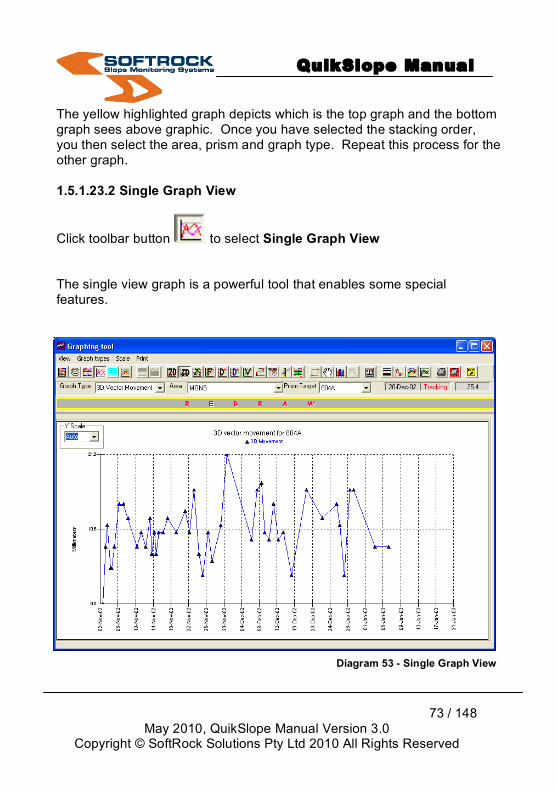
Click toolbar button to select Single Graph View The single view graph is a powerful tool that enables some special features.

Diagram 53 - Single Graph View

QuikSlope Manual

74 / 148


Note: The graph tool can be expanded to fit your full screen by using the normal windows tools.

1.5.1.24 Tracking X & Y Values

As the cursor moves over the graph, you can view the changing values of date and Y value change. This is handy on checking values of graph elements.

1.5.1.25 Zoom In

Use the zooming button to window into any area on the graph by selecting bottom left and top right of the new window.

1.5.1.26 Redraw Graph

Use the large redraw button to redraw the complete graph.

1.5.1.27 Start Date

QuikSlope Manual

75 / 148


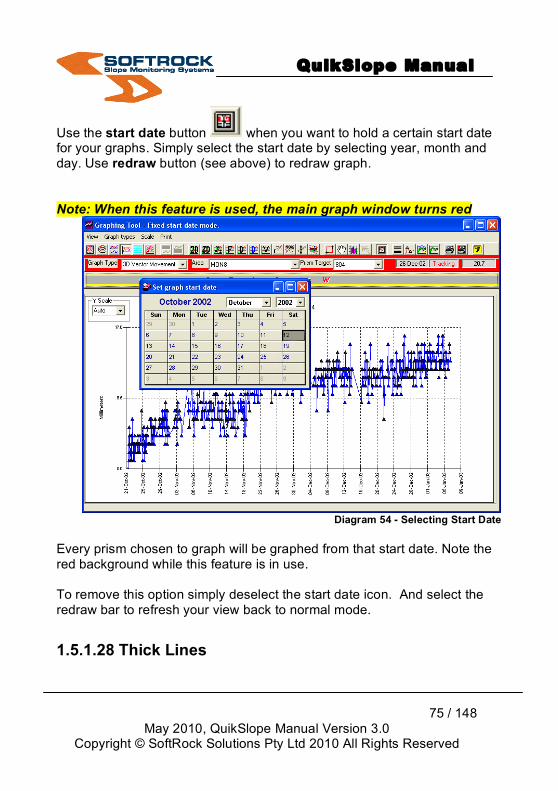
Use the start date button when you want to hold a certain start date for your graphs. Simply select the start date by selecting year, month and day. Use redraw button (see above) to redraw graph. Note: When this feature is used, the main graph window turns red

Diagram 54 - Selecting Start Date

Every prism chosen to graph will be graphed from that start date. Note the red background while this feature is in use. To remove this option simply deselect the start date icon. And select the redraw bar to refresh your view back to normal mode.

1.5.1.28 Thick Lines

QuikSlope Manual

76 / 148


Use the button to toggled on and off thick lines.

Diagram 55 - Thin Line example

Diagram 56 - Thick line example

1.5.1.29 Symbols

Use the Symbols toggle button to toggle symbols on and off. You may have to apply this button more than once for this function to work.

Diagram 57 - Symbols On

Diagram 58 - Symbols off

QuikSlope Manual

77 / 148


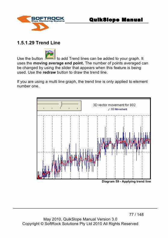
1.5.1.29 Trend Line

Use the button to add Trend lines can be added to your graph. It uses the moving average end point. The number of points averaged can be changed by using the slider that appears when this feature is being used. Use the redraw button to draw the trend line. If you are using a multi line graph, the trend line is only applied to element number one.

Diagram 59 - Applying trend line

QuikSlope Manual

78 / 148


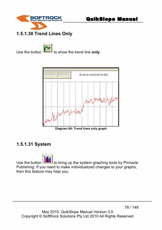
1.5.1.30 Trend Lines Only

Use the button to show the trend line only.

Diagram 60- Trend lines only graph

1.5.1.31 System

Use the button to bring up the system graphing tools by Pinnacle Publishing. If you need to make individualized changes to your graphs, then this feature may help you.

QuikSlope Manual

79 / 148


Diagram 61 - Graph Tool

1.5.1.32 View Data

Use the button to immediately view data for the current prism. Data can be edited and a line of data can be erased by highlighting the line by clicking on the left hand tab on that line. The line will be highlighted. Use the delete key on your keyboard. See remove spikes below.

QuikSlope Manual

80 / 148


Diagram 62 - View Data

1.5.1.33 Remove Spikes 1.5.1.33.1 Removing single spike You can remove a single spike in the following manner.

1. See the graph with the spike while viewing graphs in Single (or stacked) graph view.

2. Select the data view button.

3. Find the data line that is causing the problem. This is usually quite obvious. It may also be data that has not yet been calculated.

4. Highlight the problem line by clicking on the left hand tab on that line. The line will be highlighted. Use the delete key on your keyboard.

QuikSlope Manual

81 / 148


5. Check the graph by selecting the view graph button. 1.5.1.33.2 Setting limits by areas • You can also set limits by areas for deleting multiple points

1. Select the graph type adjusted distance or 3D movement 2. Enter a maximum allowable limit 3. Enter the minimum allowable limit 4. Delete the spikes outside the limits using the icon. This will delete

the points from the database, you cannot retrieve this information. 5. The limits will remain in QuikSlope until you change them.

• Or you click on the button . You must enter the maximum allowable limit for the graph, this will be a positive value in mm. Enter the minimum allowable limit for the graph, this will be a negative. These limits will remain in the database until you change them. These limits will be shown by a shaded area on your graph.

1.5.1.33.3 Show Auto Spike Delete Limits

By selecting the Auto Delete Icon , the limits that are set will be displayed. Note: If the limits set are too large for the graph in question you might need to change the limits to a smaller range.

QuikSlope Manual

82 / 148


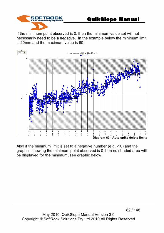
If the minimum point observed is 0, then the minimum value set will not necessarily need to be a negative. In the example below the minimum limit is 20mm and the maximum value is 60.

Diagram 63 - Auto spike delete limits

Also if the minimum limit is set to a negative number (e.g. -10) and the graph is showing the minimum point observed is 0 then no shaded area will be displayed for the minimum, see graphic below.

QuikSlope Manual

83 / 148


Diagram 64 - Graph with negative limit

Deselect the button in order to remove the shaded areas from view. 1.5.1.33.4 Delete Spike Outside Limits Once you are happy with the limits set for this graph, select the Delete

Spike Outside Limits icon . Every point within this shaded area will be deleted. They are permanently removed from the database, so use this option with care.

QuikSlope Manual

84 / 148


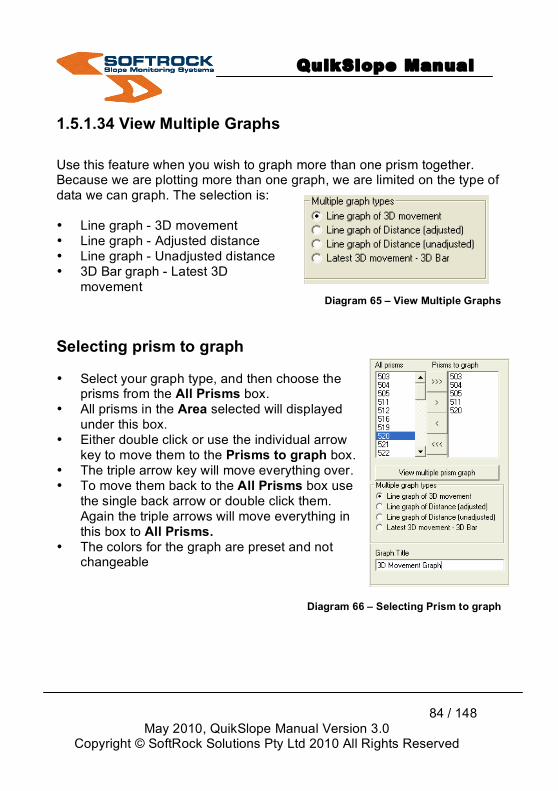
1.5.1.34 View Multiple Graphs Use this feature when you wish to graph more than one prism together. Because we are plotting more than one graph, we are limited on the type of data we can graph. The selection is: • Line graph - 3D movement • Line graph - Adjusted distance • Line graph - Unadjusted distance • 3D Bar graph - Latest 3D

movement Diagram 65 – View Multiple Graphs

Selecting prism to graph • Select your graph type, and then choose the

prisms from the All Prisms box. • All prisms in the Area selected will displayed

under this box. • Either double click or use the individual arrow

key to move them to the Prisms to graph box. • The triple arrow key will move everything over. • To move them back to the All Prisms box use

the single back arrow or double click them. Again the triple arrows will move everything in this box to All Prisms.

• The colors for the graph are preset and not changeable

Diagram 66 – Selecting Prism to graph

QuikSlope Manual

85 / 148


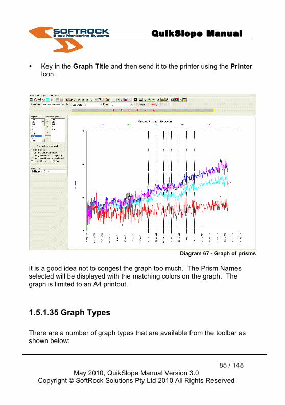
• Key in the Graph Title and then send it to the printer using the Printer

Icon.

Diagram 67 - Graph of prisms

It is a good idea not to congest the graph too much. The Prism Names selected will be displayed with the matching colors on the graph. The graph is limited to an A4 printout.

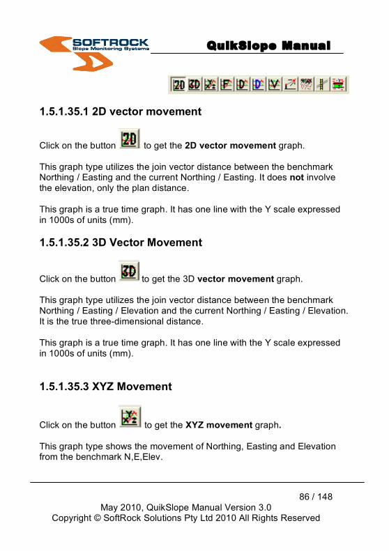
1.5.1.35 Graph Types There are a number of graph types that are available from the toolbar as shown below:

QuikSlope Manual

86 / 148


1.5.1.35.1 2D vector movement

Click on the button to get the 2D vector movement graph. This graph type utilizes the join vector distance between the benchmark Northing / Easting and the current Northing / Easting. It does not involve the elevation, only the plan distance. This graph is a true time graph. It has one line with the Y scale expressed in 1000s of units (mm). 1.5.1.35.2 3D Vector Movement

Click on the button to get the 3D vector movement graph. This graph type utilizes the join vector distance between the benchmark Northing / Easting / Elevation and the current Northing / Easting / Elevation. It is the true three-dimensional distance. This graph is a true time graph. It has one line with the Y scale expressed in 1000s of units (mm). 1.5.1.35.3 XYZ Movement

Click on the button to get the XYZ movement graph. This graph type shows the movement of Northing, Easting and Elevation from the benchmark N,E,Elev.

QuikSlope Manual

87 / 148


This graph is a true time graph. It has three lines for X, Y and Z movements. The Y scale expressed in 1000s of units (mm). 1.5.1.35.4 Adjusted Field Data

Click on the button to get the Adjusted Field Data graph. This graph type shows the difference of Horiz angle, Vert angle, and Slope distance. These are the three basic elements of the actual data measured in the field. This data is Northing, Easting and Elevation from the benchmark N,E,Elev. This graph is a true time graph. It has three lines for X, Y and Z movements. The Y scale expressed in 1000s of units (mm). 1.5.1.35.5 Unadjusted Distance

Click on the button to get the Unadjusted Distance graph. This graph type shows the difference of the unadjusted slope distance. The unadjusted distance is the actual measured field distance. This graph is a true time graph. It has one line for distance movement. The Y scale expressed in 1000s of units (mm). 1.5.1.35.6 Adjusted Distance

Click on the button to get the Adjusted Distance graph. This graph type shows the difference of the adjusted slope distance. The adjusted distance is the actual measured field distance multiplied by the distance factor.

QuikSlope Manual

88 / 148


The distance factor is a calculated scale factor found when comparing the measured distance to the REF prism with the design distance. This graph is a true time graph. It has one line for distance movement. The Y scale expressed in 1000s of units (mm). 1.5.1.35.7 Distances Adjusted & Unadjusted This graph type shows the difference of the adjusted and unadjusted slope distances. The unadjusted distance is the actual measured field distance. The adjusted distance is the actual measured field distance multiplied by the distance factor. The distance factor is a calculated scale factor found when comparing the measured distance to the REF prism with the design distance. This graph is a true time graph. It has two lines for each distance movement. The Y scale is expressed in 1000s of units (mm). Note: This Graph is handy in checking what effect the adjustments are having on your calculated prism xyz positions. 1.5.1.35.8 Velocity SD

Click on the button to get the Velocity SD graph. SD Velocity calculation is based on the adjusted measured distance difference from the previous reading extrapolated out to a 24-hour day. In other words, mm per day. If at 10:00 AM the distance was 678.908 and at 11:00 AM the distance was 678.910, then the velocity is calculated at (2mm per 2 hours or expressed as a velocity of 24mm/day. NOTE: The above value could be misleading.

QuikSlope Manual

89 / 148


To minimise extrapolations from readings of only a few hours apart, AutoSlope will hunt for the last reading taken at least 24 hours ago. Otherwise velocities can be exaggerated when taken over short time spans.

NOTE : This must be understood for fast moving prisms. SD velocity makes sense when the distance measured from the instrument station is in the expected direction of the prism movement. In other words, be sure that if you depend on this method that your prism is measured from the opposite side of the pit. If not, then the 2D velocity may be a better option. SD Velocity is the most accurate but only accounts for one direction of movement. Velocity is calculated using the adjusted distance value, compared with the previous value, and using the time between readings to extract the value in mm/day. 1.5.1.35.9 Velocity 2D 2D Velocity calculation is based on the calculated XY position difference from the previous XY position extrapolated out to a 24-hour day. In other words, mm per day. If at 10:00AM and 12 NOON the XY join distance was 3mm then the velocity is calculated at (3mm x 24hours / 2hours) = 36mm/day. NOTE: Again, the above value can be misleading. Therefore AutoSlope will hunt for the last reading taken at least 24 hours ago. Otherwise velocities can be exaggerated when taken over short time spans. Note: that this velocity may not be as accurate as the SD velocity because it depends on a calculated distance between calculated XY positions in time. The SD velocity is based on distance, which is the

QuikSlope Manual

90 / 148


most accurate field measurement. The 2D velocity is a calculation on a calculation. Use 2D velocity when the direction of measurement is not directly across the pit but from an obtuse angle. 1.5.1.35.10 Velocity 2D & SD A good rule of thumb is to put in a low SD velocity (e.g. 5) and a higher 2D velocity (e.g. 35). This should then pick up the accurate changes of distance but also get the other movement directions from the rougher 2D velocity. Unless there is a need, it is recommended that you do not use 3D movement. 1.5.1.35.11 Control Check

Click on the button to get the Control Check graph. This graph shows data that can be very handy in assessing if there is movement in your control. It assumes that if the distance factor (scale factor) that is applied to the distance is staying pretty constant, then the distance to the REF is probably constant. If the factor is trending up or down, then we are applying an increasing distance factor over time. This graph is a true time graph. It has two lines distance factor (SF) and Vertical angle factor (in seconds). The vertical angle factor applies to your levels and works in the same manner except it is expressed in units of seconds. NOTE: Do not forget to check the adjusted distance and unadjusted distance graph.

QuikSlope Manual

91 / 148


1.5.1.35.12 Rainfall

Click on the button to get the Rainfall graph. Data can be entered into the rainfall database by date and gauge reading. This graph is a true time graph. It has one line for gauge reading. The Y scale expressed in 1000s of units (mm). 1.5.1.35.13 Rainfall & Adjusted Distance Data can be entered into the rainfall database by date and gauge reading. This graph will show both gauge readings and adjusted distance. This graph is a true time graph. It has two lines for gauge reading and distance movement. The Y scale expressed in 1000s of units (mm). 1.5.1.35.14 AutoWeather Rain If you are running the AutoWeather program then data will be automatically entered into the Weather database. This graph is a true time graph. It has one line for gauge reading. The Y scale expressed in 1000s of units (mm). 1.5.1.35.15 AutoWeather & Adjusted Distance If you are running the AutoWeather program then data will be automatically entered into the Weather database. This graph will show both gauge readings and adjusted distance. This graph is a true time graph. It has two lines for gauge reading and distance movement. The Y scale expressed in 1000s of units (mm).

QuikSlope Manual

92 / 148


1.5.1.35.16 Crack Movement

Click on the button to get the Crack Movement graph. Data can be entered into the crack database by date and reading. This graph will show both crack readings and adjusted distance. This graph is a true time graph. It has two lines for gauge reading and distance movement. The Y scale expressed in 1000s of units (mm). 1.5.1.35.17 Crack & Rainfall Data can be entered into the rainfall database by date and gauge reading. Data can also be entered into the crack database by date and reading. This graph will show both crack readings and rain gauge reading. This graph is a true time graph. It has two lines for gauge reading and crack movement. The Y scale expressed in 1000s of units (mm). 1.5.1.35.18 Seismic Data

Click on the button to get the Seismic Data graph. Data can be entered into the seismic database by date and Richter scale reading. This graph is a true time graph. It has one line for Richter reading. The Y scale expressed in units

1.5.1.36 Graph Operations

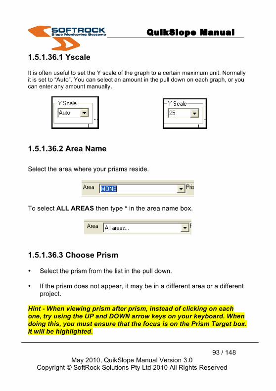
QuikSlope Manual

93 / 148


1.5.1.36.1 Yscale It is often useful to set the Y scale of the graph to a certain maximum unit. Normally it is set to “Auto”. You can select an amount in the pull down on each graph, or you can enter any amount manually.

1.5.1.36.2 Area Name

Select the area where your prisms reside.

To select ALL AREAS then type * in the area name box.

1.5.1.36.3 Choose Prism • Select the prism from the list in the pull down. • If the prism does not appear, it may be in a different area or a different

project. Hint - When viewing prism after prism, instead of clicking on each one, try using the UP and DOWN arrow keys on your keyboard. When doing this, you must ensure that the focus is on the Prism Target box. It will be highlighted.

QuikSlope Manual

94 / 148


1.5.1.36.4 Printing

Click on the button for printing. There are two ways to print: 1. Single print of current plot or graph 2. Batch printing of a number of graphs. 1.5.1.36.5 Batch Print

Click on the button for batch printing. Use this feature to print all the graphs in an area. You can print both stacked and single graphs. Things you may want to think about before printing are:

1. Are the prisms in the correctly area name?

2. Does the area name reflect the part of the project you wish to show?

3. Do you want to hold a Yscale for all plots. Auto Yscale is handy but can be confusing when looking at a lot of printed graphs. Holding a particular Yscale (maximum Y) is often a good idea before starting to run batch prints. You may have to flip through the prisms (See section 1.5.1.36.3 Choose prism) to check out what value would be best for you.

Steps for batch printing:

QuikSlope Manual

95 / 148


1. Click on batch print button

2. Select printer from Windows printer dialog box.

3. Warning window will appear showing number of prints appears. Click yes to continue.

4. Window will appear showing if you wish to view an auto flip through the graphs to check Y scale or whatever. Each graph can be viewed for 2 seconds automatically. Click yes to view graphs or No to skip this step.

5. Confirmation message will appear for continuing printing or not. Click Yes to perform the printing.

QuikSlope Manual

96 / 148


1.5.1.37 Removing Spikes From time to time you might experience a Spike in your data, where an erroneous reading causes the graph to form a flat line apart form one reading. These Spikes can be removed using the three buttons provided as shown below.

NOTE: Please ensure that you are using 3D Vector Graph or Adjusted Distance Graph only.

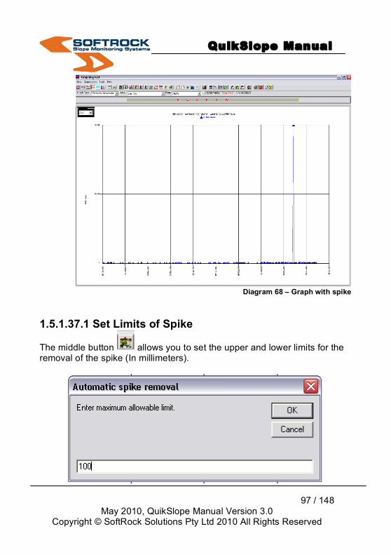
QuikSlope Manual

97 / 148


Diagram 68 – Graph with spike

1.5.1.37.1 Set Limits of Spike

The middle button allows you to set the upper and lower limits for the removal of the spike (In millimeters).

QuikSlope Manual

98 / 148


1.5.1.37.2 Show Auto Spike Delete Limits

The first button shows you a graphical display on your graph of the limits that you have set. The hatched area being the area where the points will be deleted.

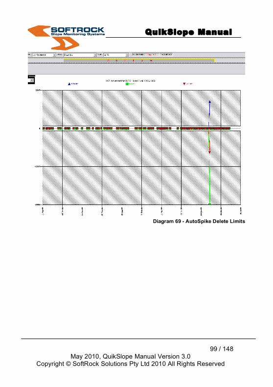
QuikSlope Manual

99 / 148


Diagram 69 - AutoSpike Delete Limits

QuikSlope Manual

100 / 148


1.5.1.37.3 Delete Spike Outside Limit

The third button will delete the points that fall inside the hatched area

Press Yes to proceed

QuikSlope Manual

101 / 148


Diagram 70 - Graph with deleted spike

1.5.2 Prism Reports

Click on the button to view prism reports. Prism reports allow you to printout actual data from the database. You can select from seven different types of report, from the drop down menu.

QuikSlope Manual

102 / 148


Diagram 71 - Report Writer

The different reports available are: 1. Setup Data: This general report shows all the setup data for each

setup number, including adjustments applied by using the reference prism and the ppm (if recorded.)

2. Prism Field Data (Requires a target to be selected): This is a report specific to a particular Target ID. It shows all raw data, adjusted data, standard deviation of filed readings and number of shots taken.

3. Prism Coordinates (Requires a target to be selected). Again this is a

Target ID specific report. It shows all calculated coordinates, calculated movements xyz, and calculated vectors.

4. Prism Vectors & Velocities: This report will print the movements (or vectors) of the raw data, coordinates, xyz vectors, and velocities.

5. Events: All events are shown from the event database.

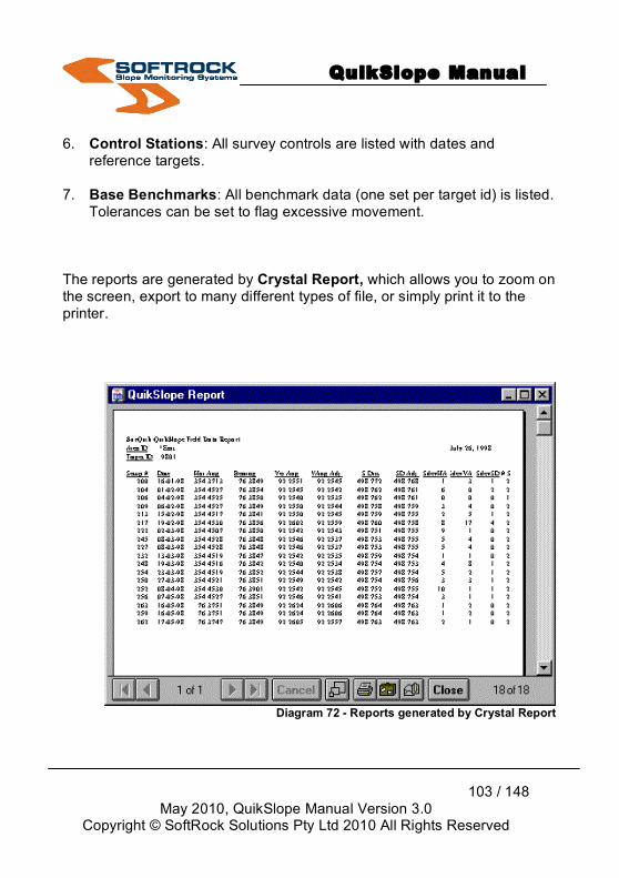
QuikSlope Manual

103 / 148


6. Control Stations: All survey controls are listed with dates and

reference targets. 7. Base Benchmarks: All benchmark data (one set per target id) is listed.

Tolerances can be set to flag excessive movement.

The reports are generated by Crystal Report, which allows you to zoom on the screen, export to many different types of file, or simply print it to the printer.

Diagram 72 - Reports generated by Crystal Report

QuikSlope Manual

104 / 148


1.5.3 Create Export File for Spreadsheets

Diagram 73 Reporting & Exporting dropdown menu

This feature allows the user to export data to a spreadsheet via a CSV (comma-delimited) file. There is an Excel macro available to automatically graph target data. The file is created by area, so select an area and filename before starting. Note: Remember the file will be saved directly into the configuration directory.

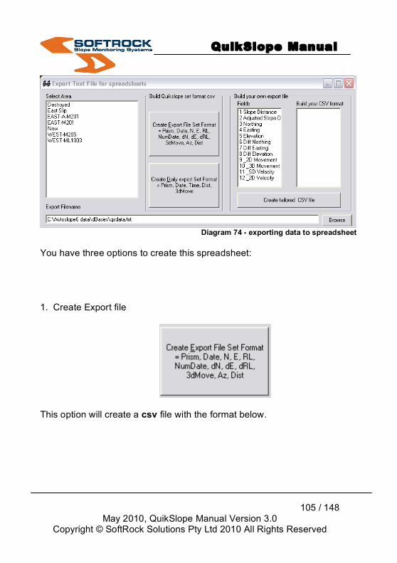
QuikSlope Manual

105 / 148


Diagram 74 - exporting data to spreadsheet

You have three options to create this spreadsheet: 1. Create Export file

This option will create a csv file with the format below.

QuikSlope Manual

106 / 148


Diagram 75 - Export file format

. 3. Create Daily Export file

This option will create a csv file with the format below.

Diagram 76 - Daily export file format

3. Build your own export file

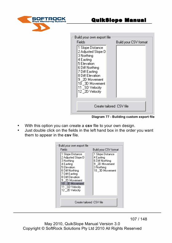
QuikSlope Manual

107 / 148


Diagram 77 - Building custom export file

• With this option you can create a csv file to your own design. • Just double click on the fields in the left hand box in the order you want

them to appear in the csv file.

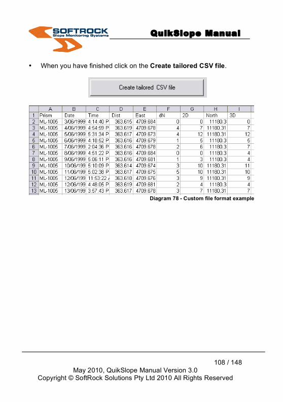
QuikSlope Manual

108 / 148


• When you have finished click on the Create tailored CSV file.

Diagram 78 - Custom file format example

QuikSlope Manual

109 / 148


1.5.4 Export Plot Data File (Surpac)

Diagram 79 - Export plot data file options

The coordinate listing for each Target ID will be written to an ASCII file in the Surpac format. This format is 2 header lines and then each data line is:

string number (1), y, x, z, Target ID All targets are written for a particular area name. There are two options: 1. Create Target Coordinate File. 2. Create Enhanced Scatter Coordinate File.

1.5.4.1 Create Target Coordinate File

Diagram 80 - Creating Target Coordinate file

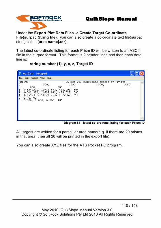
QuikSlope Manual

110 / 148


Under the Export Plot Data Files -> Create Target Co-ordinate File(surpac String file), you can also create a co-ordinate text file(surpac string called [area name].str). The latest co-ordinate listing for each Prism ID will be written to an ASCII file in the surpac format. This format is 2 header lines and then each data line is:

string number (1), y, x, z, Target ID

Diagram 81 - latest co-ordinate listing for each Prism ID

All targets are written for a particular area name(e.g. if there are 20 prisms in that area, then all 20 will be printed in the export file). You can also create XYZ files for the ATS Pocket PC program.

QuikSlope Manual

111 / 148


Diagram 82 - Creating XYZ file

Simply select XYZ handheld from the File type option and the [area name].xyz file will be created.

Diagram 83 - XYZ file example

This is a unique file that contains a particular group of prisms. All prism groups have the extension xyz. The format of this file is Prism name, Northing, Easting, RL delimited by commas. See the example WindowNo1.xyz below.

QuikSlope Manual

112 / 148


1.5.4.2 Create Enhanced Scatter Co-ordinate File The second file you can create is the scatter co-ordinate file. Choose the Area you wish to write to file and the area name.str file will be created. You can change this name and directory if you so wish.

Diagram 84 - Exporting scatter string file

The information that is written to this file is the Benchmark data for all prisms, the last position observed and all intermediate points that exist in that area.

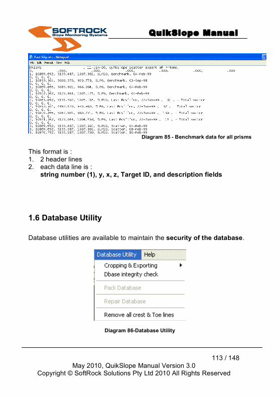
QuikSlope Manual

113 / 148


Diagram 85 - Benchmark data for all prisms

This format is : 1. 2 header lines 2. each data line is :

string number (1), y, x, z, Target ID, and description fields

1.6 Database Utility Database utilities are available to maintain the security of the database.

Diagram 86-Database Utility

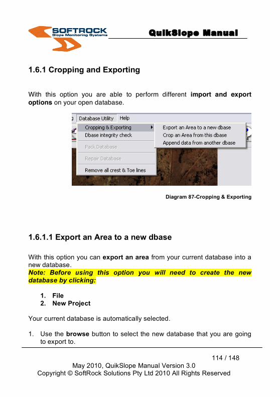
QuikSlope Manual

114 / 148


1.6.1 Cropping and Exporting

With this option you are able to perform different import and export options on your open database.

Diagram 87-Cropping & Exporting

1.6.1.1 Export an Area to a new dbase With this option you can export an area from your current database into a new database. Note: Before using this option you will need to create the new database by clicking:

1. File 2. New Project

Your current database is automatically selected. 1. Use the browse button to select the new database that you are going

to export to.

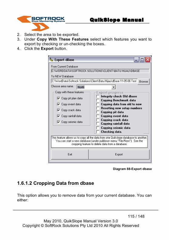
QuikSlope Manual

115 / 148


2. Select the area to be exported. 3. Under Copy With These Features select which features you want to

export by checking or un-checking the boxes. 4. Click the Export button.

Diagram 88-Export dbase

1.6.1.2 Cropping Data from dbase This option allows you to remove data from your current database. You can either:

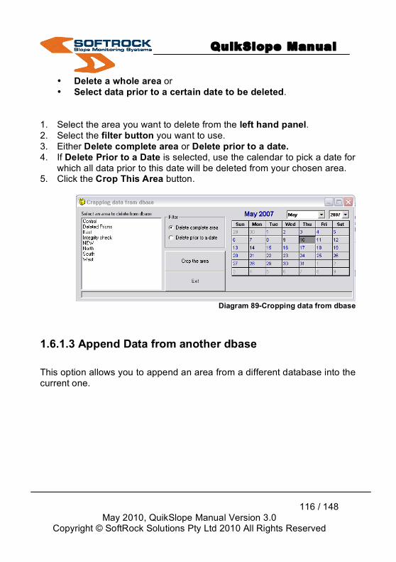
QuikSlope Manual

116 / 148


• Delete a whole area or • Select data prior to a certain date to be deleted.

1. Select the area you want to delete from the left hand panel. 2. Select the filter button you want to use. 3. Either Delete complete area or Delete prior to a date. 4. If Delete Prior to a Date is selected, use the calendar to pick a date for

which all data prior to this date will be deleted from your chosen area. 5. Click the Crop This Area button.

Diagram 89-Cropping data from dbase

1.6.1.3 Append Data from another dbase This option allows you to append an area from a different database into the current one.

QuikSlope Manual

117 / 148


Diagram 90-Append Data

1. Use the Browse button to select the database that you want to copy

from. 2. Select the area. 3. Click Append The Area Data button.

1.6.2 Database Integrity Check The database integrity check will make sure that all the Prism target names have a benchmark listing. If they do not, they will be placed in an Area file called Integrity check. Prisms with no setup data found will be deleted. It can be performed occasionally.

1.6.3 Pack Database

This feature will delete all erased files in the database and can create a database of considerably less size.

1.6.4 Repair Database

QuikSlope Manual

118 / 148


If you are having problems with accessing data in the database, the file could be corrupted. It is good practice to keep a backup. However, you can often repair a damaged database with this feature. Note: Repairing and packing is done automatically each day.

1.6.5 Remove all Crest and Toe Lines

Sometimes very large files are accidentally loaded into your database. This option will remove all crest and toe lines from your database. Note: It is prudent to keep pit files under 100 000 points. Please backup your database before proceeding with this action.

1.7 Help

Online help is available while using QuikSlope.

Diagram 91-Help

1.7.1 About About is about the latest version and software registration particulars.

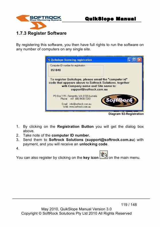
QuikSlope Manual

119 / 148


1.7.3 Register Software By registering this software, you then have full rights to run the software on any number of computers on any single site.

Diagram 92-Registration

1. By clicking on the Registration Button you will get the dialog box

above. 2. Take note of the computer ID number. 3. Send them to Softrock Solutions ([email protected]) with

payment, and you will receive an unlocking code. 4.

You can also register by clicking on the key icon on the main menu.

QuikSlope Manual

120 / 148


Part C QuikSlope - First User Guide The normal sequence of events is: 1. Download the field data file. 2. Vet the field data and merge it with the main database. 3. Ensure the control data is entered including the reference target

prisms. 4. Calculate the set-ups. 5. Enter the Benchmark values for each prism. 6. Calculate the movements. See calculate coordinates. (Do this after

changing the base readings) This calculation is usually done automatically in the calc setup, but has to be done manually first up.

1.8 First Time Check List After starting QuikSlope for the first time, you should be aware of: Registered or unregistered user. QuikSlope is shipped as a 30 day demo but can be upgraded to a registered version by sending your codes to Softrock Solutions. See the dialog box under the pull-down menu Help Register Software. You only need to upgrade before the 30-day trial period expires. Start a Project. All data in QuikSlope is saved as an Access database in the file format *.mdb. When QuikSlope is shipped to you, it uses a database called demo.mdb. It is important to start a new project for your site. The project name will always appear in the title strip of the main window of QuikSlope. So under pull-down menu click on: 1. File 2. New Project to create a new file in your working directory for slope

monitoring data.

QuikSlope Manual

121 / 148


(This file can be accessed from any computer on the network running QuikSlope.)

Import Data You may wish to start with data that you have already collected. You can import coordinate data by using pull down menu and selecting: 1. Data Import 2. Import Coordinate-only data.

This will allow you to import an ASCII file in the format Point ID, Date, Northing, Easting, Elevation.

1.8.1 Field Procedures (Manually)

1. Set up the instrument. 2. Record the instrument set-up data and date. 3. Take shots to all target, and reference prisms. Use both faces and get

at least 2 shots per target. 4. Record Target ID, Horiz Angle, Vert Angle, and Slope distance. 5. Be careful to record the correct target ID.

Note: Try to use the same procedure each time, although the order of shots is not important.

1.8.2 Field Data 1. Start QuikSlope

2. Use the Field Data menu option. Choose the data-type from

Geodimeter, Leica, Sokkia, Nikon, or Topcon.

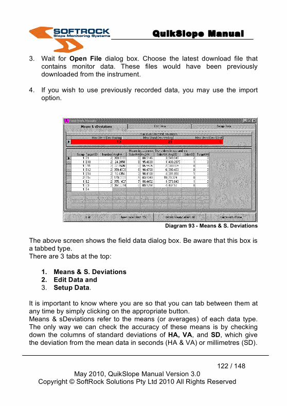
QuikSlope Manual

122 / 148


3. Wait for Open File dialog box. Choose the latest download file that contains monitor data. These files would have been previously downloaded from the instrument.

4. If you wish to use previously recorded data, you may use the import option.

Diagram 93 - Means & S. Deviations

The above screen shows the field data dialog box. Be aware that this box is a tabbed type. There are 3 tabs at the top:

1. Means & S. Deviations 2. Edit Data and 3. Setup Data.

It is important to know where you are so that you can tab between them at any time by simply clicking on the appropriate button. Means & sDeviations refer to the means (or averages) of each data type. The only way we can check the accuracy of these means is by checking down the columns of standard deviations of HA, VA, and SD, which give the deviation from the mean data in seconds (HA & VA) or millimetres (SD).

QuikSlope Manual

123 / 148


Note: You cannot edit this page directly. You have to tab to the next page and edit the data if any looks bad. Note the data in red at the top of the page. This is the maximum standard deviation for each column, i.e. HA, VA and SD.

1.8.3 Edit Data This data has to be edited and recalculated to change the means and standard deviations. Firstly, let us look at the items in this dialog box: • The setup item refers to the setup number in this particular file and has

no relation to the unique setup number used later in the calculation phase.

• The HA and VA is in decimal degrees and sometimes is shown as a negative HA.

• The status is set to 1 for all manual instruments and is set to show successful signal return in robotic operations.

All data can be edited directly. It is often as simple as an incorrect target ID for a set of readings. It may be necessary to delete a whole record. To do this: 1. Click any cell on that record 2. Click the left hand marker button for the row (or record) so that the

complete row is highlighted 3. Hit the delete key on your keyboard.

QuikSlope Manual

124 / 148


Diagram 94 - Editing Data Note: Do not forget to use the Recalc Means after Edit before tabbing back to the Means & Standard Deviations tab. • When the standard deviations are at a desirable level: Use the Merge with dbase button to send the mean data only to the main database. • If the standard deviations are still large:

Then select the Edit data tab and proceed with further edits. Note: The Standard deviations should be as close to zero as possible. (You might need to go through this editing a number of times before this is achieved.)

QuikSlope Manual

125 / 148


Diagram 95 – Ensuring S. Deviations are close to zero

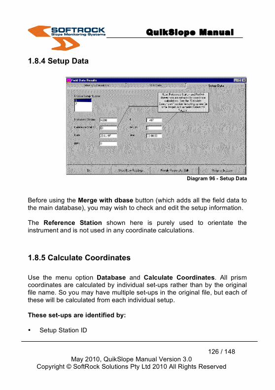
QuikSlope Manual

126 / 148


1.8.4 Setup Data

Diagram 96 - Setup Data

Before using the Merge with dbase button (which adds all the field data to the main database), you may wish to check and edit the setup information. The Reference Station shown here is purely used to orientate the instrument and is not used in any coordinate calculations.

1.8.5 Calculate Coordinates Use the menu option Database and Calculate Coordinates. All prism coordinates are calculated by individual set-ups rather than by the original file name. So you may have multiple set-ups in the original file, but each of these will be calculated from each individual setup. These set-ups are identified by: • Setup Station ID

QuikSlope Manual

127 / 148


• Setup ID (a unique number) used by the database. • Setup Date • Round ID is a name used by robotics or download file name for manual

operations.

1.8.6 Calculation Procedure

1. Select the Instrument Setup Station in the list box provided. 2. Wait till the setup data appears on the screen. (Any uncalculated set-

ups will appear as the default, but you may select to show all set-ups.) 3. When choosing a setup, watch the setup data to know you have the

correct one. 4. Use the Calculate this Setup button to proceed with the actual calc. 5. (Any adjustments used are shown on the message box below. The

vertical adjustment is shown as an angle in degrees.mmss and the distance adjustment is shown in metres to 4 decimal places. Both these figures are the adjustment over 1000 metres and will be pro-rated over each individual slope distance.)

6. By using the YES button, the calculation will proceed. 7. Continue until all set-ups are calculated.

1.8.7 Setup Station Data

During the calculation processes above, you may check and change the setup data. This data includes: • The Hor Ang Reference Target. This is the control point (reference

prism) to be used for all bearing calculations.

QuikSlope Manual

128 / 148


• The Vert Ang Reference Target. This is the control point (reference prism) to be used for vertical angle calculations. This can be switched off with the check box.

• The Distance Reference Target. This is the control point (reference prism) to be used for all distance calculations. It is simply used to apply a scale factor. This can be switched off with the check box.

Use the Calculate Adjustment Factors button to check these adjustment factors at any time. The Vertical adjustment will be shown as a vertical angle (ddd.mmss) per 1000 metres. So for a distance of 500 metres only half of this angular correction will be applied. The slope distance correction is shown as a distance per 1000 metres. The horizontal correction refers to the difference to bearings. This is not optional.

1.8.8 Control Coordinates

1. Use Calculations and Survey Control Database menu options to view and edit control data.

2. Either

i. Select an existing control point from the listing, Or

ii. Use the Add control point button.

(You will firstly be prompted to select a Control Point as shown in the dialog box below.) Remember to include all instrument stations and reference targets (prisms). Note: You can have multiple listings of the one control point. Ensure that your earliest date is earlier (or the same) than the date of the first set of readings.

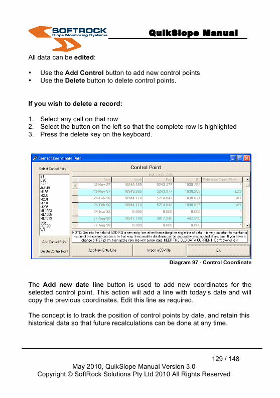
QuikSlope Manual

129 / 148


All data can be edited: • Use the Add Control button to add new control points • Use the Delete button to delete control points. If you wish to delete a record: 1. Select any cell on that row 2. Select the button on the left so that the complete row is highlighted 3. Press the delete key on the keyboard.

Diagram 97 - Control Coordinate

The Add new date line button is used to add new coordinates for the selected control point. This action will add a line with today’s date and will copy the previous coordinates. Edit this line as required. The concept is to track the position of control points by date, and retain this historical data so that future recalculations can be done at any time.

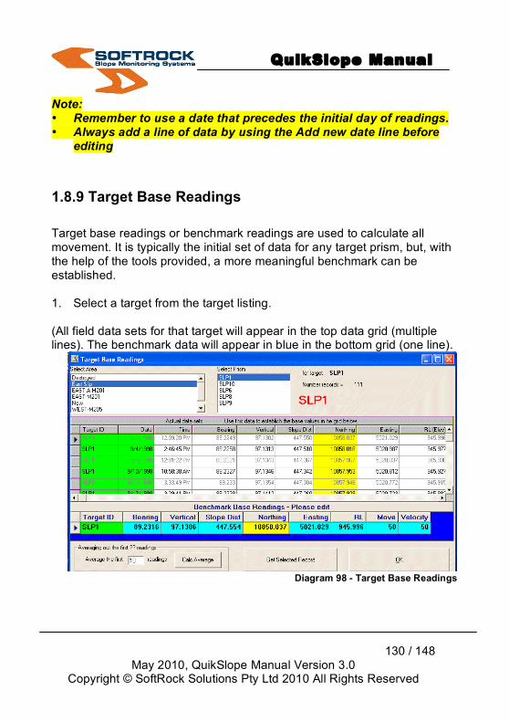
QuikSlope Manual

130 / 148


Note: • Remember to use a date that precedes the initial day of readings. • Always add a line of data by using the Add new date line before

editing

1.8.9 Target Base Readings Target base readings or benchmark readings are used to calculate all movement. It is typically the initial set of data for any target prism, but, with the help of the tools provided, a more meaningful benchmark can be established. 1. Select a target from the target listing.

(All field data sets for that target will appear in the top data grid (multiple lines). The benchmark data will appear in blue in the bottom grid (one line).

Diagram 98 - Target Base Readings

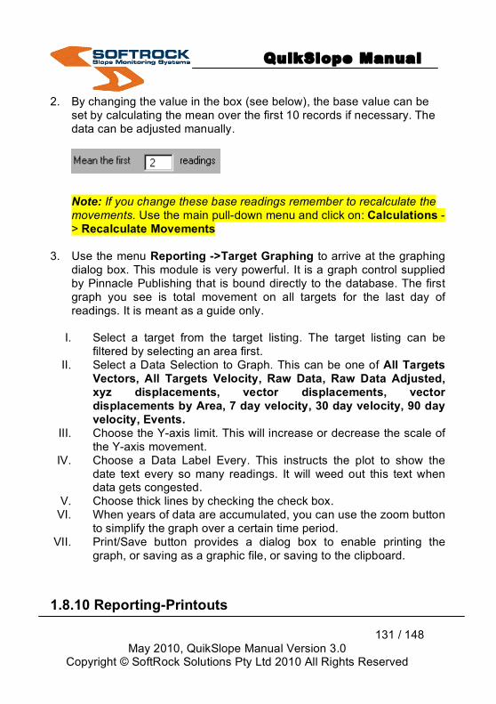
QuikSlope Manual

131 / 148


2. By changing the value in the box (see below), the base value can be set by calculating the mean over the first 10 records if necessary. The data can be adjusted manually.

Note: If you change these base readings remember to recalculate the movements. Use the main pull-down menu and click on: Calculations -> Recalculate Movements

3. Use the menu Reporting ->Target Graphing to arrive at the graphing

dialog box. This module is very powerful. It is a graph control supplied by Pinnacle Publishing that is bound directly to the database. The first graph you see is total movement on all targets for the last day of readings. It is meant as a guide only.

I. Select a target from the target listing. The target listing can be

filtered by selecting an area first. II. Select a Data Selection to Graph. This can be one of All Targets

Vectors, All Targets Velocity, Raw Data, Raw Data Adjusted, xyz displacements, vector displacements, vector displacements by Area, 7 day velocity, 30 day velocity, 90 day velocity, Events.

III. Choose the Y-axis limit. This will increase or decrease the scale of the Y-axis movement.

IV. Choose a Data Label Every. This instructs the plot to show the date text every so many readings. It will weed out this text when data gets congested.

V. Choose thick lines by checking the check box. VI. When years of data are accumulated, you can use the zoom button

to simplify the graph over a certain time period. VII. Print/Save button provides a dialog box to enable printing the

graph, or saving as a graphic file, or saving to the clipboard.

1.8.10 Reporting-Printouts

QuikSlope Manual

132 / 148


This concerns those who require the hard copy of the actual data or who want to check some problem in field data or calculations. This option will create Crystal Reports, which have many powerful options. Data can be sent in many different file formats. There are many report types available. To create the history of all the observed data in this report simply: 1. Select the report type

and 2. Choose the Area, and the Prism in

Question.

Diagram 99-Report Types

Diagram 100 - Choosing area and prism

QuikSlope Manual

133 / 148


Note: The report types Events, Control Stations, Base Benchmarks and Setup Data gives does not require you to select the Area or Prism number.

Diagram 101 – QuikSlope Report

1.8.11 Creating CSV File Before exiting QuikSlope, the option to create the qsdata.txt file is to be used. Under the menu item Reporting & Exporting, click on: Create Export File for Spreadsheets. 1. Select the Area 2. Use the Create Export File button to create the text file.

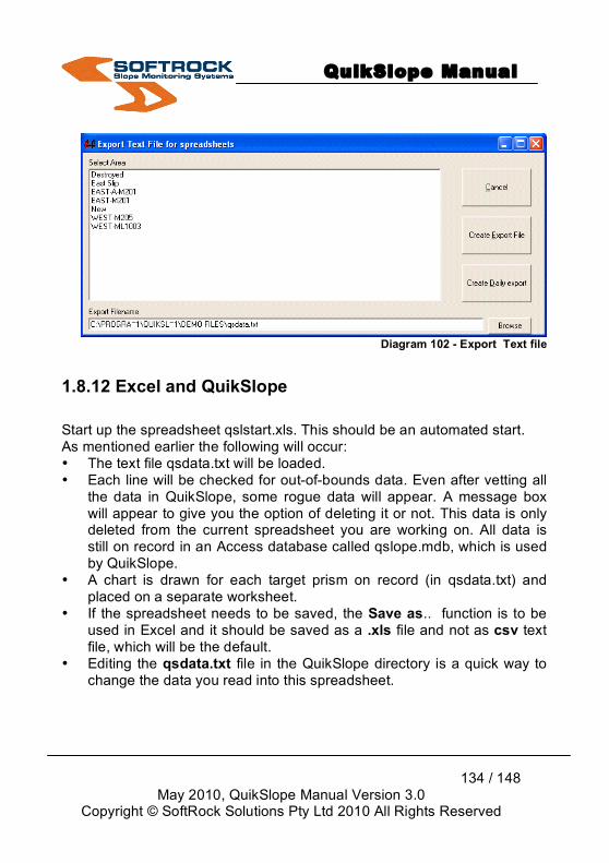
QuikSlope Manual

134 / 148


Diagram 102 - Export Text file

1.8.12 Excel and QuikSlope Start up the spreadsheet qslstart.xls. This should be an automated start. As mentioned earlier the following will occur: • The text file qsdata.txt will be loaded. • Each line will be checked for out-of-bounds data. Even after vetting all

the data in QuikSlope, some rogue data will appear. A message box will appear to give you the option of deleting it or not. This data is only deleted from the current spreadsheet you are working on. All data is still on record in an Access database called qslope.mdb, which is used by QuikSlope.

• A chart is drawn for each target prism on record (in qsdata.txt) and placed on a separate worksheet.

• If the spreadsheet needs to be saved, the Save as.. function is to be used in Excel and it should be saved as a .xls file and not as csv text file, which will be the default.

• Editing the qsdata.txt file in the QuikSlope directory is a quick way to change the data you read into this spreadsheet.

QuikSlope Manual

135 / 148


Part D Terminology 1.9 Graphing Terminology 1.9.1 XYZ Movement XYZ movement consists of 3 graph lines. Three individual movements of northing, easting and elevation (RL). The movements are calculated from the benchmark Northing, Easting and Elevation.

Note: Remember to adjust the benchmark figures if the graphs look strange. Any adjustments of benchmark data will require a recalculation of delta movements.

1.9.2 XYZ Vector Movement XYZ vector movement consists of 1 graph line. Single vector 3D distance being calculated from the benchmark northing, easting and elevation. Note: Remember to adjust the benchmark figures if the graphs look strange. Any adjustments of benchmark data will require a recalculation of delta movements.

1.9.3 Unadjusted Distance Unadjusted distance consists of 1 graph line. Field distance as read from the instrument. Note: Remember to adjust the benchmark figures if the graphs look strange. Any adjustments of benchmark data will require a recalculation of delta movements.

1.9.4 Adjusted Field Data Adjusted field data consists of 3 graph lines. Field measurements from the instrument are adjusted by use of the reference target. Horizontal angles are adjusted to bearings, vertical angles are adjusted, and slope distances are adjusted. See how adjustment is applied under Calculations.

QuikSlope Manual

136 / 148


Note: Remember to adjust the benchmark figures if the graphs look strange. Any adjustments of benchmark data will require a recalculation of delta movements.

1.9.5 Adjusted Distance Adjusted distance consists of 1 graph line. Field slope distance is adjusted by using of the reference target. See how adjustment is applied under Calculations. Note: Remember to adjust the benchmark figures if the graphs look strange. Any adjustments of benchmark data will require a recalculation of delta movements.

1.9.6 Distance and Adjustment Factor Distance and adjustment factor consists of 2 graph lines. Field slope distance is adjusted by using of the reference target. The resultant adjustment factor is represented by xx millimetres per 1000 metres. Note: Graphing this factor together with the distance is the best way of checking on the actual movement of reference targets or control points. A regularly changing adjustment factor could indicate that your control needs checking. Control being station points and reference prisms. (See how adjustment is applied under Calculations). Note: Remember to adjust the benchmark figures if the graphs look strange. Any adjustments of benchmark data will require a recalculation of delta movements.

QuikSlope Manual

137 / 148


1.9.7 7 Day Velocity 7-Day velocity consists of 2 graph lines. Velocity is produced by: 1. Calculating the xyz vector movement, 2. Dividing it by the number of days since the benchmark and 3. Multiplying by 7.

A trend line is added from this data. Note: Remember to adjust the benchmark figures if the graphs look strange. Any adjustments of benchmark data will require a recalculation of delta movements.

1.9.8 30 Day Velocity 30-Day velocity consists of 2 graph lines. Velocity is produced by 1. Calculating the xyz vector movement, 2. Dividing it by the number of days since the benchmark and 3. Multiplying by 30. 4. A trend line is added from this data. Note: Remember to adjust the benchmark figures if the graphs look strange. Any adjustments of benchmark data will require a recalculation of delta movements.

1.9.9 90 Day Velocity 90-Day velocity is 2 graph lines. Velocity is produced by 1. Calculating the xyz vector movement, 2. Dividing it by the number of days since the benchmark and 3. Multiplying by 90.

QuikSlope Manual

138 / 148


A trend line is added from this data. Note: Remember to adjust the benchmark figures if the graphs look strange. Any adjustments of benchmark data will require a recalculation of delta movements.

1.10 QuikSlope Terminology

1.10.1 Reference Prism The reference prism should be placed so that when you measure to it, it is measuring through the same column of air as the target prisms. Then you can take advantage of the full adjusting features of QuikSlope. All calculations are based on the accuracy of the instrument station and the reference prism.

1.10.2 Benchmark Benchmark data is the original set of readings that all graphing and movement calculations are based.

1.10.3 Setup Number Setup number is a unique number that is generated by the computer. It cannot be changed. It is the link between Instrument Setup information and the Target data. Note: It is not to be confused with Instrument or Setup ID.

QuikSlope Manual

139 / 148


1.10.4 Target ID A target ID refers to the name of the actual prism target set in the wall of the open pit or area of suspected movement. This name can be a unique alphanumeric label.

1.10.5 Area Name Area Names are used to group prisms into areas. Damaged prisms can still be kept on file by keeping them under an Area Name like Destroyed. Note that the default area name for new Targets is New.

QuikSlope Manual

140 / 148


1.11 Instruments 1.11.1 Robotic Instruments Geodimeter ATS and Leica have robotic instruments that will automatically measure to a group of prisms. See SurQuik Software’s ATS program that controls the Geodimeter by direct cable or radio link.

1.11.2 Topcon Data Format The following is the Topcon format: JOB# NAME INST# DATE 17/07/97 OCC.ST# M200 ID INS.HT 1.487 PT# E1 H +0000000d V +0885148d PCODE BS R.HT 0.000 PT# M193 H +0000722d V +0893632d SD +00479884m PCODE 1 R.HT 0.000 PT# E1 H +3595956d V +0885148d SD +00549955m

QuikSlope Manual

141 / 148


PCODE 1 R.HT 0.000 PT# E2 H +3551414d V +0884506d SD +00573847m PCODE 1 R.HT 0.000

1.11.3 Wild Leica File Format Wild Leica File Format can be in either 8 or 16 bit versions and both will automatically be recognised. 8-bit file: 110001+00STN501 84..10+10000000 85..10+20000000 86..10+00500000 87..10+00000000 88..10+00001345 79....+00STN502 110002+0PRISM01 21.324+12635520 22.324+09227350 31..00+00007138 87..10+00000000 81..00+10005726 82..00+19995748 83..00+00501039 110003+0PRISM01 21.324+12635520 22.324+09227350 31..00+00007138 87..10+00000000 81..00+10005726 82..00+19995748 83..00+00501039 110008+0PRISM02 21.324+32905180 22.324+26545260 31..00+00005084 87..10+00000000 81..00+10002605 82..00+19995650 83..00+00500969 110009+0PRISM02 21.324+32905190 22.324+26545260 31..00+00005084 87..10+00000000 81..00+10002605 82..00+19995650 83..00+00500969 110014+0PRISM03 21.324+17138120 22.324+08240340 31..00+00010654 87..10+00000000 81..00+10001537 82..00+19989545 83..00+00502703 110015+0PRISM03 21.324+17138130 22.324+08240340 31..00+00010654 87..10+00000000 81..00+10001537 82..00+19989545 83..00+00502703

16-bit file: *110001+0000000000STN501 84..10+0000000010000000 85..10+0000000020000000 86..10+0000000000500000 87..10+0000000000000000 88..10+0000000000001345 79....+0000000000STN502 *110002+000000000PRISM01 21.324+0000000016710480 22.324+0000000009227350 31..00+0000000000007138

QuikSlope Manual

142 / 148


87..10+0000000000000000 81..00+0000000010001582 82..00+0000000019993046 83..00+0000000000501039 *110003+000000000PRISM01 21.324+0000000016710490 22.324+0000000009227340 31..00+0000000000007138 87..10+0000000000000000 81..00+0000000010001582 82..00+0000000019993046 83..00+0000000000501039 *110008+000000000PRISM02 21.324+0000000000940400 22.324+0000000026545300 31..00+0000000000005084 87..10+0000000000000000 81..00+0000000009999148 82..00+0000000019995002 83..00+0000000000500969 *110009+000000000PRISM02 21.324+0000000000940400 22.324+0000000026545300 31..00+0000000000005084 87..10+0000000000000000 81..00+0000000009999148 82..00+0000000019995002 83..00+0000000000500969 *110014+000000000PRISM03 21.324+0000000021214100 22.324+0000000008240290 31..00+0000000000010655 87..10+0000000000000000 81..00+0000000009994363 82..00+0000000019991061 83..00+0000000000502704 22.324+0000000008240300 31..00+0000000000010655 87..10+0000000000000000 81..00+0000000009994363 82..00+0000000019991061 83..00+0000000000502704

1.11.4 Geodimeter File Format Geodimeter file format should include the following:

50=PIT Filename

2=M201 Station Name

3=0.263 Height Inst

62=ML1003 Ref Object (Optional. This is not required for calculating coordinates.)

21=125.0602 HA Ref (This is also optional because it is also not required.)

30=1 ppm. (Optional but is recorded in dbase as a check on field distances

51=14/07/98 Date

52=15:52:26 Time

5=9401 Target Name

QuikSlope Manual

143 / 148


6=0 Signal Ht

7=108.0348 Hor Ang

8=97.3905 Vert Ang

9=459.195 Slope distance

1.11.5 Geodimeter Servo Driven Procedures A. Creating Geodimeter Area File Creating an area file of prism coordinates will allow the servo driven instruments to roughly point to the prism to be monitored. These coordinates should be accurate enough to find the prism. B. Geodimeter Program Setup Ensure that the Geodimeter is setup to record the following data in the job file when using Program 23. To setup the data: 1. Hold the program key down for over 1 second. 2. Scroll through to Program 23 3. Hold the program key down for over 1 second. 4. Then enter the following:-

Label Number Prompt 51 Date 52 Time 30 ppm 5 Pno 6 Sh 7 HA 8 VA 9 SD

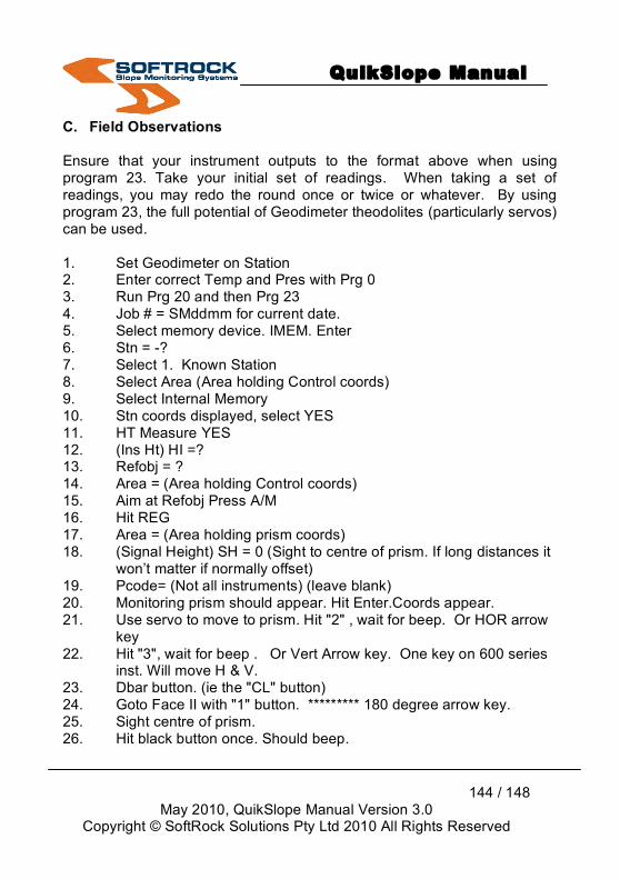
QuikSlope Manual

144 / 148


C. Field Observations Ensure that your instrument outputs to the format above when using program 23. Take your initial set of readings. When taking a set of readings, you may redo the round once or twice or whatever. By using program 23, the full potential of Geodimeter theodolites (particularly servos) can be used. 1. Set Geodimeter on Station 2. Enter correct Temp and Pres with Prg 0 3. Run Prg 20 and then Prg 23 4. Job # = SMddmm for current date. 5. Select memory device. IMEM. Enter 6. Stn = -? 7. Select 1. Known Station 8. Select Area (Area holding Control coords) 9. Select Internal Memory 10. Stn coords displayed, select YES 11. HT Measure YES 12. (Ins Ht) HI =? 13. Refobj = ? 14. Area = (Area holding Control coords) 15. Aim at Refobj Press A/M 16. Hit REG 17. Area = (Area holding prism coords) 18. (Signal Height) SH = 0 (Sight to centre of prism. If long distances it

won’t matter if normally offset) 19. Pcode= (Not all instruments) (leave blank) 20. Monitoring prism should appear. Hit Enter.Coords appear. 21. Use servo to move to prism. Hit "2" , wait for beep. Or HOR arrow

key 22. Hit "3", wait for beep . Or Vert Arrow key. One key on 600 series

inst. Will move H & V. 23. Dbar button. (ie the "CL" button) 24. Goto Face II with "1" button. ********* 180 degree arrow key. 25. Sight centre of prism. 26. Hit black button once. Should beep.

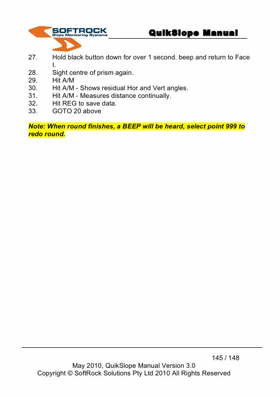
QuikSlope Manual

145 / 148


27. Hold black button down for over 1 second. beep and return to Face I.

28. Sight centre of prism again. 29. Hit A/M 30. Hit A/M - Shows residual Hor and Vert angles. 31. Hit A/M - Measures distance continually. 32. Hit REG to save data. 33. GOTO 20 above

Note: When round finishes, a BEEP will be heard, select point 999 to redo round.

QuikSlope Manual

146 / 148


Appendix Diagrams Diagram 1 – Regional and Language Options ............................................... 7 Diagram 2 - Customizing Short Date Format ................................................. 8 Diagram 3 - Correct Short Date Format.......................................................... 8 Diagram 4 - Main Pull-Down Menu – Toolbar .............................................. 13 Diagram 5 - File Menu.................................................................................... 13 Diagram 8 - Edit pull-down menu .................................................................. 22 Diagram 9 - Edit Setup Table ........................................................................ 23 Diagram 10 - Edit Prism Table....................................................................... 24 Diagram 12 - Delete Prism............................................................................. 27 Diagram 13 - Delete by Instrument Setup Number ...................................... 28 Diagram 14 – Area Name for: Import ............................................................ 29 Diagram 15 - Editing Bench Marks................................................................ 30 Diagram 16 - Target Base Readings............................................................. 32 Diagram 17 - Event Database ....................................................................... 33 Diagram 18 - Prism Name Editor................................................................... 34 Diagram 19 - List of Prism Names ................................................................ 35 Diagram 20 - Rainfall...................................................................................... 35 Diagram 21 - Crack monitors menus ............................................................ 36 Diagram 22 - Crack Monitor Master List ....................................................... 36 Diagram 23 - Crack Monitor Readings.......................................................... 37 Diagram 24 - Seismic Activity ........................................................................ 39 Diagram 25 - Calculations drop-down menu ................................................ 40 Diagram 26 - Field Layout.............................................................................. 40 Diagram 27 - Calculate coordinates .............................................................. 42 Diagram 28 - Calculated coordinates............................................................ 44 Diagram 29 - Setup Station Data................................................................... 45 Diagram 30 - Calculate Adjustment Factors................................................. 46 Diagram 31 - Using Curvature and Refraction ............................................. 47 Diagram 32 - Control Coordinate Data Form................................................ 49 Diagram 33 - G1S01 Table ............................................................................ 51 Diagram 34 - Recalculate Movements .......................................................... 52 Diagram 35 - Global Calculation Options ..................................................... 53 Diagram 36 - Example of temp-qs.txt............................................................ 54 Diagram 37 -Grid Conversion Form .............................................................. 56 Diagram 38 - Reporting Dropdown Menu ..................................................... 57

QuikSlope Manual

147 / 148


Diagram 39 - 24-hour report .......................................................................... 59 Diagram 40 - Various graph views options ................................................... 59 Diagram 41 - Graph View ............................................................................. 60 Diagram 42 - A4 Plan Plot ............................................................................ 60 Diagram 43 - Location Plot ........................................................................... 61 Diagram 44 - Stacked Graph ........................................................................ 61 Diagram 45 - Graph Data.............................................................................. 61 Diagram 46 - Multiple Prism Graphs ............................................................ 62 Diagram 47 - A4 Plan Plot ............................................................................. 63 Diagram 48 - Scatter plots ............................................................................. 67 Diagram 49 - Example of Logo ...................................................................... 68 Diagram 50 - Location and scatter form........................................................ 69 Diagram 51 - Stacked Graph Views .............................................................. 72 Diagram 52 - Toggle Graph Views ................................................................ 72 Diagram 54 - Selecting Start Date................................................................. 75 Diagram 55 - Thin Line example ................................................................... 76 Diagram 56 - Thick line example ................................................................... 76 Diagram 57 - Symbols On.............................................................................. 76 Diagram 59 - Applying trend line ................................................................... 77 Diagram 60- Trend lines only graph .............................................................. 78 Diagram 61 - Graph Tool ............................................................................... 79 Diagram 62 - View Data ................................................................................. 80 Diagram 63 - Auto spike delete limits............................................................ 82 Diagram 64 - Graph with negative limit......................................................... 83 Diagram 65 – View Multiple Graphs.............................................................. 84 Diagram 66 – Selecting Prism to graph ........................................................ 84 Diagram 67 - Graph of prisms ....................................................................... 85 Diagram 68 – Graph with spike ..................................................................... 97 Diagram 69 - AutoSpike Delete Limits .......................................................... 99 Diagram 70 - Graph with deleted spike.......................................................101 Diagram 71 - Report Writer ..........................................................................102 Diagram 72 - Reports generated by Crystal Report...................................103 Diagram 73 Reporting & Exporting dropdown menu .................................104 Diagram 74 - exporting data to spreadsheet ..............................................105 Diagram 75 - Export file format....................................................................106 Diagram 76 - Daily export file format...........................................................106 Diagram 77 - Building custom export file ....................................................107 Diagram 78 - Custom file format example ..................................................108

QuikSlope Manual

148 / 148


Diagram 79 - Export plot data file options...................................................109 Diagram 80 - Creating Target Coordinate file.............................................109 Diagram 81 - latest co-ordinate listing for each Prism ID ..........................110 Diagram 82 - Creating XYZ file....................................................................111 Diagram 83 - XYZ file example....................................................................111 Diagram 84 - Exporting scatter string file....................................................112 Diagram 85 - Benchmark data for all prisms ..............................................113 Diagram 86-Database Utility ........................................................................113 Diagram 87-Cropping & Exporting ..............................................................114 Diagram 88-Export dbase ............................................................................115 Diagram 89-Cropping data from dbase.......................................................116 Diagram 90-Append Data ............................................................................117 Diagram 91-Help...........................................................................................118 Diagram 92-Registration ..............................................................................119 Diagram 93 - Means & S. Deviations ..........................................................122 Diagram 94 - Editing Data............................................................................124 Diagram 95 – Ensuring S. Deviations are close to zero ............................125 Diagram 96 - Setup Data .............................................................................126 Diagram 97 - Control Coordinate.................................................................129 Diagram 98 - Target Base Readings...........................................................130 Diagram 99-Report Types............................................................................132 Diagram 100 - Choosing area and prism....................................................132 Diagram 101 – QuikSlope Report ...............................................................133 Diagram 102 - Export Text file ....................................................................134

quikslope manual module 1 - members.iinet.net.aumembers.iinet.net.au/~softrock/support/module 1 -...

Documents