purchasing power parity and the taylor rule · purchasing power parity and the taylor rule...
TRANSCRIPT

Purchasing Power Parity and the Taylor Rule
Hyeongwoo Kim∗ and Masao Ogaki†
January 2011
Abstract
In the Kehoe and Midrigan (2007) model, the persistence parameter of the real exchange rate is closely
related to the measure of price stickiness in the Calvo-pricing model. When we employ this view, Rogoff’s
(1996) 3 to 5 year consensus half-life implies that firms update their prices every 18 to 30 quarters on
average. This is at odds with most estimates from U.S. aggregate data when single equation methods are
applied to the New Keynesian Phillips Curve (NKPC), or when system methods are applied to Dynamic
Stochastic General Equilibrium (DSGE) models that include the NKPC. It is well known, however, that
there is a large degree of uncertainty around the consensus half-life of the real exchange rate. To obtain
a more efficient estimator, this paper develops a system method that combines the Taylor rule and a
standard exchange rate model to estimate half-lives. We use a median unbiased estimator for the system
method with nonparametric bootstrap confidence intervals, and compare the results with those from the
single equation method typically used in the literature. Applying the method to the real exchange rates of
18 developed countries against the U.S. dollar, we find that most of the half-life estimates from the single
equation method fall in the range of 3 to 5 years with wide confidence intervals that extend to positive
infinity. In contrast, the system method yields median-unbiased estimates that are typically shorter than
one year with much sharper 95% confidence intervals, most of which range from 3 quarters to 5 years.
These median unbiased estimates and the lower bound of the confidence intervals for the half-lives of real
exchange rates are consistent with most estimates of price stickiness using aggregate U.S. data for the
NKPC and DSGE models.
Keywords: Purchasing Power Parity, Calvo Pricing, Taylor Rule, Half-Life of PPP Deviations, Median
Unbiased Estimator, Grid-t Confidence Interval
JEL Classification: C32, E52, F31
∗Corresponding Author: Hyeongwoo Kim, Department of Economics, Auburn University, 0339 Haley Center., Auburn, AL36849. Tel: 1-334-844-2928. Fax: 1-334-844-4615. Email: [email protected]
†Department of Economics, Keio University, 612 Mita-Kenkyu-shitsu 2-15-45 Mita Minato-ku, Tokyo, 108-8345, Japan. Tel:81-3-5418-6403. Fax: 81-3-5427-1578. Email: [email protected]
1

1 Introduction
Reviewing the literature on Purchasing Power Parity (PPP), Rogoff (1996) found, using single
equation methods, a remarkable consensus on 3 to 5 year half-life estimates of real exchange
rate deviations from PPP. This is an important piece of Rogoff’s "PPP puzzle" as the question
of how one might reconcile highly volatile short-run movements of real exchange rates with an
extremely slow convergence rate to PPP. This puzzle can be described in the context of the New
Keynesian model with Calvo pricing. For example, Galí and Gertler (1999) use U.S. aggregate
data, the unit labor cost and CPI, to estimate the New Keynesian Phillips curve (NKPC). Their
preferred estimate implies that the average frequency of the price change is about 5 quarters.
On the other hand, a single-good version of Kehoe and Midrigan’s (2007) model can be used to
find the implication of the 3 to 5 year half-life estimates from real exchange rate data for the
same average pricing frequency (see Section 2 below). They imply 18 to 30 quarters. Thus, it
is hard to reconcile Galí and Gertler’s result with the extremely slow convergence rate found
in Rogoff’s remarkable consensus.
Using Rogoff’s remarkable consensus as the starting point, many possible solutions to the
PPP puzzle have been proposed in the literature.1 One important example is Imbs, Mumtaz,
Ravn, and Rey (2005), who point out that sectoral heterogeneity in convergence rates can
cause upward bias in half-life estimates, and claim that this aggregation bias explains the PPP
puzzle. While it is possible that the bias can solve the PPP puzzle under certain conditions,
it is also possible that the bias is negligible under other conditions. For example, Chen and
Engel (2005), Crucini and Shintani (2008), and Parsley and Wei (2007) have found negligible
aggregation biases. Broda and Weinstein (2008) show that the aggregation bias of the form
that Imbs, Mumtaz, Ravn, and Rey (2005) studied is small for their barcode data, even though
the convergence coefficient rises as they move to aggregate indexes. These papers are about
purely statistical findings.
Another delicate issue is how we should aggregate micro evidence of price stickiness for
dynamic aggregate models, such as dynamic stochastic general equilibrium (DSGE) models,
which Carvalho and Nechio (2008) have started to study. Thus, even though the aggregation
bias is an important possibility, much more research seems necessary before we reach a consensus
on whether or not the aggregation bias solves the PPP puzzle, and how we should aggregate
for DSGE models.1See Murray and Papell (2002) for a discussion of other solutions which take Rogoff’s remarkable consensus
as a starting point.
2

In this paper, we ask a different question: Should we really take Rogoff’s remarkable con-
sensus of 3-5 year half-life estimates as the starting point for the aggregate CPI data? The
consensus may at first seem to support the reliability of these estimates, but Kilian and Zha
(2002), Murray and Papell (2002), and Rossi (2005) have shown that the degree of uncertainty
around these point estimates is huge. Murray and Papell (2002) conclude that singe equation
methods provide virtually no information regarding the size of half-lives. Therefore, it is not
clear if the true half-lives are as slow as Rogoff’s remarkable consensus implies. If we apply a
more efficient estimator to the real exchange rate data, we may find much faster convergence
rates.
For the purpose of obtaining a more efficient estimator, we develop a system method that
combines the Taylor rule and a standard exchange rate model in order to estimate the half-life
of the real exchange rate. Several recent papers have provided empirical evidence in favor of
exchange rate models with Taylor rules (see Mark 2005, Engel and West 2005, 2006, Clarida
and Waldman 2007, Molodtsova and Papell 2007, and Molodtsova, Nikolsko-Rzhevskyy and
Papell 2008). Therefore, a system method using an exchange rate model with the Taylor rule
is a promising way to try to improve on single equation methods to estimate the half-lives.
Because standard asymptotic theory usually does not provide adequate approximations for
the estimation of half-lives of real exchange rates, we use a nonparametric bootstrap method to
construct confidence intervals. Median unbiased estimates based on the bootstrap are reported.
As we review in Section 5 below, the contrast between the single equation methods and our
system method, in the context of PPP literature, corresponds with the contrast between single
equation methods for the NKPC and system methods for DSGE models with the NKPC in
the literature for closed economy models. Single equation methods such as Galí and Gertler’s
(1999) GMM yield small standard errors for the average price duration based on standard
asymptotic theory. However, Kleibergen andMavroeidis (2009), who take into account the weak
identification problem of GMM, report that the upper bound of their 95% confidence interval
for the price duration is infinity. The estimators of average price duration in system methods
for DSGE models in Christiano, Eichenbaum, and Evans (2005) and Smets and Wouters (2007),
among others, may be more efficient.
We apply the system method to estimate the half lives of real exchange rates of 18 developed
countries against the U.S. dollar. Most of the estimates from the single equation method fall
in the range of 3 to 5 years, with wide confidence intervals that extend to positive infinity. In
contrast, the system method yields median unbiased estimates that are typically substantially
3

shorter than 3 years with much sharper confidence intervals, most of which range from three
quarters to 5 years.
In the recent papers of two-country exchange rate models with Taylor rules cited above, the
authors assume that Taylor rules are adopted by the central banks of both countries. Because
Taylor rules may not be used by some countries, we only assume that the Taylor rule is used by
the home country, and remain agnostic about the monetary policy rule in the foreign country.
None of these papers with Taylor rules estimates half-lives of real exchange rates.
Kim and Ogaki (2004), Kim (2005), and Kim, Ogaki, and Yang (2007) use system methods
to estimate half-lives of real exchange rates. However, they use conventional monetary models
without Taylor rules based on money demand functions. Another important difference of these
works from the present paper is that their inferences are based on asymptotic theory, while
ours is based on the grid bootstrap.
The rest of the paper is organized as follows. Section 2 describes our baseline model.
We construct a system of stochastic difference equations for the exchange rate and inflation,
explicitly incorporating a forward looking Taylor rule into the system. Section 3 explains our
estimation methods. In Section 4, we report our empirical results. Section 5 reviews the current
empirical NKPC literature in relation to our findings. Section 6 concludes.
2 The Model
2.1 Gradual Adjustment Equation
We start with a univariate stochastic process of real exchange rates. Let pt be the log domestic
price level, p∗t be the log foreign price level, and et be the log nominal exchange rate as the
price of one unit of the foreign currency in terms of the home currency. And we denote st as
the log of the real exchange rate, p∗t + et − pt.
We assume that PPP holds in the long-run. Putting it differently, we assume that there
exists a cointegrating vector [1 − 1 − 1]0 for a vector [pt p∗t et]0, where pt, p∗t , and et are dif-
ference stationary processes. Under this assumption, the real exchange rate can be represented
as the following stationary univariate autoregressive process of degree one.
st+1 = d+ αst + εt+1, (1)
where α is a positive persistence parameter that is less than one.
4

Admittedly, estimating half-lives of real exchange rates with an AR(1) specification may not
be ideal, because the AR(1) model is mis-specified and will lead to an inconsistent estimator if
the true data generating process is a higher order autoregressive process, AR(p). It is interesting
to see, however, that Rossi (2005) reported similar half-life estimates from both models. Later
in Section 4, we confirm that this is roughly the case for our exchange rate data. Thus, assuming
AR(1) seems innocuous for the purpose of estimating the half life of most real exchange rates
in our data. A different issue is whether or not the assumption of AR(1) is appropriate for
other purposes such as examining the shape of the impulse responses (Steinsson, 2008). Even
though this is an interesting question, we do not pursue this issue in the current paper.
Recently, Kehoe and Midrigan (2007) show that the persistence parameter α is closely
related to a measure of price stickiness in Calvo (1983) pricing models. It can be shown that a
single-good version of their model implies the stochastic process (1) for the real exchange rate
where α equals the probability that firms do not adjust their prices in any given period. Along
the line of Woodford (2007), Kim (2009) shows that (1) can be also derived from a similar
model as Kehoe and Midrigan’s (2007) with the Taylor Rule.
By rearranging and taking conditional expectations, the equation (1) can be written by
the following error correction model of real exchange rates with a known cointegrating relation
described earlier.
Et∆pt+1 = b [μ− (pt − p∗t − et)] + Et∆p∗t+1 + Et∆et+1, (2)
where μ = E(pt − p∗t − et), b = 1 − α, d = −(1 − α)μ, εt+1 = ε1,t+1 + ε2,t+1 − ε3,t+1 =
(et+1−Etet+1)+(p∗t+1−Etp∗t+1)−(pt+1−Etpt+1), and Etεt+1 = 0. E(·) denotes the unconditionalexpectation operator while Et(·) is the conditional expectation operator on It, the economic
agent’s information set at time t.2 Note that b is the convergence rate (= 1 − α), which is a
positive constant less than unity by construction.
2.2 The Taylor Rule Model
We assume that the uncovered interest parity (UIP) holds. That is,
Et∆et+1 = it − i∗t , (3)
2A single-good version of Mussa’s (1982) model implies this when we add a domestic price shock, pt+1−Etpt+1,that has a conditional expectation of zero given the information at time t.
5

where it and i∗t are domestic and foreign interest rates, respectively.3
The central bank in the home country is assumed to continuously set its optimal target
interest rate (iTt ) by the following forward looking Taylor Rule.4
iTt = r + γπEt∆pt+1 + γxxt,
where r is a constant that includes a certain long-run equilibrium real interest rate along with
a target inflation rate5, and γπ and γx are the long-run Taylor Rule coefficients on expected
future inflation6 (Et∆pt+1) and current output deviations7 (xt), respectively. We also assume
that the central bank attempts to smooth the interest rate by the following rule.
it = (1− ρ)iTt + ρit−1,
that is, the current actual interest rate is a weighted average of the target interest rate and the
previous period’s interest rate, where ρ is the smoothing parameter. Then, we can derive the
forward looking version Taylor Rule equation with interest rate smoothing policy as follows.
it = (1− ρ)r + (1− ρ)γπEt∆pt+1 + (1− ρ)γxxt + ρit−1 (4)
Combining (3) and (4), we obtain the following.
Et∆et+1 = (1− ρ)r + (1− ρ)γπEt∆pt+1 + (1− ρ)γxxt + ρit−1 − i∗t (5)
= ι+ γsπEt∆pt+1 + γsxxt + ρit−1 − i∗t ,
3The UIP often fails to hold when one tests it by estimating a single regression equation, ∆et+1 = β(it −i∗t ) + εt+1. Therefore, it is not ideal to assume the UIP in our model, thus future research should remove thisassumption. We believe, however, that our initial attempt should start with the UIP, because it is difficult towrite an exchange rate model with the Taylor rule without the UIP for our purpose of getting more informationfrom the model. Further, Taylor rule exchange rate models in the literature often assumes the UIP.
4We remain agnostic about the policy rule of the foreign central bank, because the Taylor rule may not beemployed in some countries.
5See Clarida, Galí, and Gertler (1998, 2000) for details.6It may be more reasonable to use real-time data instead of the final release data. However, doing so will
introduce another complication as we need to specify the relation between the real-time price index and theconsumer price index, which is frequently used in the PPP literature. Hence we leave the use of real-time datafor future research.
7If we assume that the central bank responds to expected future output deviations rather than currentdeviations, we can simply modify the model by replacing xt with Etxt+1. However, this does not make anysignificant difference to our results.
6

where ι = (1− ρ)r is a constant, γsπ = (1− ρ)γπ and γsx = (1− ρ)γx are short-run Taylor Rule
coefficients.
Now, let’s rewrite (2) as the following equation in level variables.
Etpt+1 = bμ+ Etet+1 + (1− b)pt − (1− b)et + Etp∗t+1 − (1− b)p∗t (2’)
Taking differences and rearranging it, (2’) can be rewritten as follows.
Et∆pt+1 = Et∆et+1 + α∆pt − α∆et +£Et∆p∗t+1 − α∆p∗t + ηt
¤, (6)
where α = 1− b and ηt = η1,t + η2,t − η3,t = (et − Et−1et) + (p∗t − Et−1p∗t )− (pt − Et−1pt).From (4), (5), and (6), we construct the following system of stochastic difference equations.⎡⎢⎣ 1 −1 0
−γsπ 1 0
−γsπ 0 1
⎤⎥⎦⎡⎢⎣ Et∆pt+1
Et∆et+1
it
⎤⎥⎦ =⎡⎢⎣ α −α 0
0 0 ρ
0 0 ρ
⎤⎥⎦⎡⎢⎣ ∆pt
∆et
it−1
⎤⎥⎦+⎡⎢⎣ Et∆p∗t+1 − α∆p∗t + ηt
ι+ γsxxt − i∗tι+ γsxxt
⎤⎥⎦ (7)
For notational simplicity, let’s rewrite (7) in matrix form as follows.
AEtyt+1 = Byt + xt, (7’)
and thus,
Etyt+1 = A−1Byt +A−1xt (8)
= Dyt + ct,
where D = A−1B and ct = A−1xt.8 By eigenvalue decomposition, (8) can be rewritten as
follows.
Etyt+1 = VΛV−1yt + ct, (9)
where D = VΛV−1 and
V =
⎡⎢⎣ 1 1 1αγsπα−ρ 1 1αγsπα−ρ 1 0
⎤⎥⎦ , Λ =⎡⎢⎣ α 0 0
0 ρ1−γsπ
0
0 0 0
⎤⎥⎦8It is straightforward to show that A is nonsingular, and thus has a well-defined inverse.
7
Premultiplying (9) by V−1 and redefining variables,
Etzt+1 = Λzt+ht, (10)
where zt = V−1yt and ht = V−1ct.
Note that, among non-zero eigenvalues in Λ, α is between 0 and 1 by definition, whileρ
1−γsπ(= ρ
1−(1−ρ)γπ) is greater than unity as long as 1 < γπ < 1
1−ρ . Therefore, if the long-run
inflation coefficient γπ is strictly greater than one, the system of stochastic difference equations
(7) has a saddle path equilibrium, where rationally expected future fundamental variables enter
in the exchange rate and inflation dynamics.9 On the contrary, if γπ is strictly less than unity,
which might be true in the pre-Volker era in the US, the system would have a purely backward
looking solution, where the solution would be determined by past fundamental variables and
any martingale difference sequences.
Assuming γπ is strictly greater than one, we can show that the solution to (7) satisfies the
following relation (see Appendix A for the derivation).
∆et+1 = ι+αγsπα− ρ
∆pt+1 −αγsπα− ρ
∆p∗t+1 +αγsπ − (α− ρ)
α− ρi∗t (11)
+γsπ(αγ
sπ − (α− ρ))
(α− ρ)ρ
∞Xj=0
µ1− γsπ
ρ
¶j
Etft+j+1 + ωt+1,
where,
ι =αγsπ − (α− ρ)
(α− ρ)(γsπ − (1− ρ))ι,
ft = −£i∗t − Et∆p∗t+1
¤+
γsxγsπ
xt
ωt+1 =γsπ(αγ
sπ − (α− ρ))
(α− ρ)ρ
∞Xj=0
µ1− γsπ
ρ
¶j
(Et+1ft+j+1 − Etft+j+1)
+γsπ
α− ρηt+1 −
αγsπ − (α− ρ)
α− ρυt+1,
and,
Etωt+1 = 0
9The condition γπ < 11−ρ is easily met for all sample periods we consider in this paper.
8

Or, (11) can be rewritten with full parameter specification as follows.
∆et+1 = ι+αγπ(1− ρ)
α− ρ∆pt+1 −
αγπ(1− ρ)
α− ρ∆p∗t+1 +
αγπ(1− ρ)− (α− ρ)
α− ρi∗t (11’)
+γπ(1− ρ)(αγπ(1− ρ)− (α− ρ))
(α− ρ)ρ
∞Xj=0
µ1− γπ(1− ρ)
ρ
¶j
Etft+j+1 + ωt+1
Here, ft is a proxy variable that summarizes the fundamental variables such as foreign ex ante
real interest rates and domestic output deviations.
Note that if γπ is strictly less than unity, the restriction in (11) may not be valid, since the
system would have a backward looking equilibrium rather than a saddle path equilibrium.10
Put it differently, exchange rate dynamics critically depends on the size of γπ. As mentioned in
the introduction, however, we have some supporting empirical evidence for such a requirement
for the existence of a saddle path equilibrium, at least for the post-Volker era. So we believe
that our specification would remain valid for our purpose in this paper.
One related research has been recently put forward by Clarida and Waldman (2007), who
investigate exchange rate dynamics when central banks employ Taylor rules in a small open
economy framework proposed by Svensson (1999). In their paper, they derive the dynamics of
real exchange rates by combining the Taylor Rule and the uncovered interest parity (or real
interest parity), so that the real exchange rate is mainly determined by the ex ante real interest
rate. In their model, the real interest rate follows an AR(1) process of which the autoregressive
coefficient is a function of the Taylor rule coefficients. When the central bank responds to
inflation more aggressively, the economy returns to its long-run equilibrium at a faster rate.
Therefore, the half-life of PPP deviations is negatively affected by γπ.
It should be noted that their model does not explicitly incorporate the commodity view
of PPP in the sense that real exchange rate dynamics are mainly determined by the portfolio
market equilibrium conditions. Unlike them, we combine Kehoe and Midrigan’s (2007) model
with the UIP as well as the Taylor Rule. Under this framework, no policy parameters can affect
the half-life of the PPP deviations because real exchange rate persistence is mainly driven by
firms’ behavior. On the other hand, policy parameters do affect volatilities of inflation and
the nominal exchange rate in our model. For example, the more aggressively the central bank
responds to inflation, the less volatile inflation is, which leads to a less volatile nominal exchange
10If the system has a purely backward looking solution, the conventional structural Vector Autoregressive(SVAR) estimation method may apply.
9

rate.
One interesting feature arises when another policy parameter, ρ, varies. As the value for
ρ increases, the volatility of ∆pt+1 decreases. This is due to the uncovered interest parity
condition. A higher value of ρ, higher interest rate inertia, implies that the central bank
changes the nominal interest rate less. Therefore, ∆et+1 should change less due to the uncovered
interest parity. When α = ρ, it can be shown that after the initial cost-push shock, price does
not change at all (see Appendix B). That is, ∆pt+1 instantly jumps and stays at its long-run
equilibrium value of zero. Hence, the convergence toward long-run PPP should be carried over
by the exchange rate adjustments. When α < ρ, price must decrease after the initial cost-push
shock, since the nominal exchange rate movement is limited by the uncovered interest parity
and domestic interest rate inertia.
3 Estimation Methods
We discuss two estimation strategies here: a conventional univariate equation approach and the
GMM system method (Kim, Ogaki, and Yang, 2007).
3.1 Univariate Equation Approach
A univariate approach utilizes the equations (1) or (2). For instance, the persistence parameter
α in (1) can be consistently estimated by the conventional least squares method under the
maintained cointegrating relation assumption. Once we obtain the point estimate of α, the
half-life of the real exchange rate can be calculated by ln(.5)lnα
. Similarly, the regression equation
for the convergence parameter b can be constructed from (2) as follows.
∆pt+1 = b [μ− (pt − p∗t − et)] +∆p∗t+1 +∆et+1 + εt+1, (2")
where εt+1 = −εt+1 = −(et+1 − Etet+1)− (p∗t+1 − Etp∗t+1) + (pt+1 − Etpt+1) and Etεt+1 = 0.
3.2 GMM System Method
Our second estimation strategy combines the equation (11) with (1). The estimation of the
equation (11) is a challenging task, however, since it has an infinite sum of rationally expected
discounted future fundamental variables. Following Hansen and Sargent (1980, 1982), we lin-
10

early project Et(·) onto Ωt, the econometrician’s information set at time t, which is a subset of
It. Denoting Et(·) as such a linear projection operator onto Ωt, we can rewrite (11) as follows.
∆et+1 = ι+αγsπα− ρ
∆pt+1 −αγsπα− ρ
∆p∗t+1 +αγsπ − (α− ρ)
α− ρi∗t (12)
+γsπ(αγ
sπ − (α− ρ))
(α− ρ)ρ
∞Xj=0
µ1− γsπ
ρ
¶j
Etft+j+1 + ξt+1,
where
ξt+1 = ωt+1 +γsπ(αγ
sπ − (α− ρ))
(α− ρ)ρ
∞Xj=0
µ1− γsπ
ρ
¶j ³Etft+j+1 − Etft+j+1
´,
and
Etξt+1 = 0,
by the law of iterated projections.
For appropriate instrumental variables that are in Ωt, we assume Ωt = ft, ft−1, ft−2, · · · .This assumption would be an innocent one under the stationarity assumption of the fundamen-
tal variable, ft, and it can greatly lessen the burden in our GMM estimation by significantly
reducing the number of coefficients to be estimated.
Assume, for now, that ft be a zero mean covariance stationary, linearly indeterministic
stochastic process so that it has the following Wold representation.
ft = c(L)νt, (13)
where νt = ft−Et−1ft and c(L) is square summable. Assuming that c(L) = 1+c1L+c2L2+ · · ·
is invertible, (13) can be rewritten as the following autoregressive representation.
b(L)ft = νt, (14)
where b(L) = c−1(L) = 1− b1L− b2L2 − · · · . Linearly projecting
P∞j=0
³1−γsπρ
´jEtft+j+1 onto
Ωt, Hansen and Sargent (1980) show that the following relation holds.
∞Xj=0
δjEtft+j+1 = ψ(L)ft =
"1−
¡δ−1b(δ)
¢−1b(L)L−1
1− (δ−1L)−1
#ft, (15)
11
where δ = 1−γsπρ.
For actual estimation, we assume that ft can be represented by a finite order AR(r) process,
that is, b(L) = 1 −Pr
j=1 bjLj, where r < ∞.11 Then, it can be shown that the coefficients of
ψ(L) can be computed recursively (see Sargent 1987) as follows.
ψ0 = (1− δb1 − · · ·− δrbr)−1
ψr = 0
ψj−1 = δψj + δψ0bj,
where j = 1, 2, · · · , r. Then, we obtain the following two orthogonality conditions.
∆et+1 = ι+αγsπα− ρ
∆pt+1 −αγsπα− ρ
∆p∗t+1 +αγsπ − (α− ρ)
α− ρi∗t (16)
+γsπ(αγ
sπ − (α− ρ))
(α− ρ)ρ
¡ψ0ft + ψ1ft−1 + · · ·+ ψr−1ft−r+1
¢+ ξt+1,
ft+1 = k + b1ft + b2ft−1 + · · ·+ brft−r+1 + νt+1, (17)
where k is a constant scalar and Etνt+1 = 0.1213
Finally, the system method (GMM) estimation utilizes all aforementioned orthogonality
conditions, (2"), (16), and (17). That is, a GMM estimation can be implemented by the
following 2(p+ 2) orthogonality conditions.
Ex1,t(st+1 − d− αst) = 0 (18)
Ex2,t−τ
Ã∆et+1 − ι− αγsπ
α−ρ∆pt+1 +αγsπα−ρ∆p∗t+1 −
αγsπ−(α−ρ)α−ρ i∗t
−γsπ(αγsπ−(α−ρ))
(α−ρ)ρ¡ψ0ft + ψ1ft−1 + · · ·+ ψr−1ft−r+1
¢ ! = 0 (19)
Ex2,t−τ (ft+1 − k − b1ft − b2ft−1 − · · ·− brft−r+1) = 0, (20)
11We can use conventional Akaike Information criteria or Bayesian Information criteria in order to choose thedegree of such autoregressive processes.12Recall that Hansen and Sargent (1980) assume a zero-mean covariance stationary process. If the variable
of interest has a non-zero unconditional mean, we can either demean it prior to the estimation or include aconstant but leave its coefficient unconstrained. West (1989) showed that the further efficiency gain can beobtained by imposing additional restrictions on the deterministic term. However, the imposition of such anadditional restriction is quite burdensome, so we simply add a constant here.13In actual estimations, we normalized (16) by multiplying (α−ρ) to each side in order to reduce nonlinearity.
12

where x1,t = (1 st)0, x2,t = (1 ft)0, and τ = 0, 1, · · · , p.1415
3.3 Median Unbiased Estimator and Grid-t Confidence Intervals
We correct for the bias in our α estimates by a GMM version of the grid-t method proposed
by Hansen (1999) for the least squares estimator. It is straightforward to generate pseudo
samples for the orthogonality condition (20) by the conventional residual-based bootstrapping.
However, there are some complications in obtaining samples directly from (18) and (19), since
p∗t is treated as a forcing variable in our model. We deal with this problem as follows.
In order to generate pseudo samples for the orthogonality conditions (18) and (19), we
denote pt as the relative price index pt − p∗t . Then, (2") and (16) can be rewritten as follows.
∆pt+1 = bμ− b(pt − et) +∆et+1 + εt+1
∆et+1 = ι+αγsπα− ρ
∆pt+1 +αγsπ − (α− ρ)
α− ρi∗t
+γsπ(αγ
sπ − (α− ρ))
(α− ρ)ρ
¡ψ0ft + · · ·+ ψr−1ft−r+1
¢+ ξt+1
Or, in matrix form,"∆pt+1
∆et+1
#= C+ S−1
"−(1− α)
0
#[pt − et] (21)
+ S−1
⎡⎢⎣ 0αγsπ−(α−ρ)
α−ρ i∗t +γsπ(αγ
sπ−(α−ρ))
(α−ρ)ρ ·¡ψ0ft + · · ·+ ψr−1ft−r+1
¢⎤⎥⎦+ S−1 " εt+1
ξt+1
#,
where C is a vector of constants and S is∙1 − 1 ... − αγsπ
α−ρ 1
¸.
Then, treating each grid point α ∈ [αmin, αmax] as a true value, we can generate pseudosamples of ∆pt+1 and ∆et+1 by the conventional bootstrapping.16 The level variables pt and etare obtained by numerical integration. It should be noted that all other parameters are treated
14p does not necessarily coincide with r.15In actual estimations, we use the aforementioned normalization again.16The historical data were used for the initial values and the foreign interest rate i∗t .
13

as nuisance parameters (η).17 Following Hansen (1999), we define the grid-t statistic at each
grid point α ∈ [αmin, αmax] as follows.
tn(α) =αGMM − α
se(αGMM), (22)
where se(αGMM) denotes the robust GMM standard error at the GMM estimate αGMM. Imple-
menting GMM estimations for B bootstrap iterations at each of N grid point of α, we obtain
the (β quantile) grid-t bootstrap quantile functions, q∗n,β(α) = q∗n,β(α, η(α)). Note that each
function is evaluated at each grid point α rather than at the point estimate.18
Finally, we define the 95% grid-t confidence interval as follows.
α ∈ R : q∗n,2.5%(α) ≤ tn(α) ≤ q∗n,97.5%(α), (23)
and the median unbiased estimator is,
αMUE = α ∈ R, s.t. tn(α) = q∗n,50%(α) (24)
4 Empirical Results
This section reports estimates of the persistence parameter α (or convergence rate parameter
b) and their implied half-lives from the aforementioned two estimation strategies.
We use CPIs to construct real exchange rates with the US$ as a base currency. We consider
19 industrialized countries that provide 18 real exchange rates.19 For interest rates, we use
quarterly money market interest rates that are short-term interbank call rates rather than
conventional short-term treasury bill rates, since we incorporate the Taylor Rule in the model
where a central bank sets its target short-term market rate. For output deviations, we consider
two different measures of output gaps, quadratically detrended real GDP gap (see Clarida, Galí,
17See Hansen (1999) for detailed explanations.18If they are evaluated at the point estimate, the quantile functions correspond to the Efron and Tibshirani’s
(1993) bootstrap-t quantile functions.19Among 23 industrialized countries classified by IMF, we dropped Greece, Iceland, and Ireland due to lack
of reasonable number of observations. Luxembourg was not included because it has a currency union withBelgium.
14

and Gertler 1998) and unemployment rate gaps (see Boivin 2006).2021 The data frequency
is quarterly and from the IFS CD-ROM. The sample period is from 1979:III to 1998:IV for
Eurozone countries, and from 1979:III to 2003:IV for the rest of the countries.
The reason that our sample period starts from 1979.III is based on empirical evidence on
the US Taylor Rule. As discussed in Section II, the inflation and exchange rate dynamics may
greatly depend on the size of the central bank’s reaction coefficient to expected inflation. We
showed that the rationally expected future fundamental variables appear in the exchange rate
and inflation dynamics only when the long-run inflation coefficient γπ is strictly greater than
unity. Clarida, Galí, and Gertler (1998, 2000) provide important empirical evidence for the
existence of a structural break in the US Taylor Rule. Put it differently, they show that γπ was
strictly less than one during the pre-Volker era, while it became strictly greater than unity in
the post-Volker era.
We implement similar GMM estimations for (4) as in Clarida, Galí, and Gertler (2000)2223
with longer sample period and report the results in Table 1 (see the note on Table 1 for detailed
explanation). We use two output gap measures for three different sub-samples. Most coefficients
were highly significant and specification tests by J-test were not rejected.24 More importantly,
our requirement for the existence of a saddle path equilibrium met for the post-Volker era
rather than the pre-Volker era. Therefore, we may conclude that this provides some empirical
justification for the choice of our sample period.
Insert Table 1 Here
We report our GMM version median unbiased estimates and the 95% grid-t confidence
intervals in Table 2. We implemented estimations using both gap measures, but report the
full estimates with unemployment gaps in order to save space.25 We chose N = 30 and B =
20We also tried same analysis with the cyclical components of real GDP series from the HP-filter with 1600of smoothing parameter. The results were quantitatively similar.21The unemployment gap is defined as a 5 year backward moving average subtracted by the current unem-
ployment rate. This specification makes its sign consistent with that of the conventional output gap.22They used GDP deflator inflation along with the CBO output gaps (and HP detrended gaps).23Unlike them, we assume that the Fed targets current output gap rather than future deviations. However,
this doesn’t make any significant changes to our results. And we include one lag of interest rate rather thantwo lags for simplicity.24J-test statistics are available upon request.25The results with quadratically detrended real GDP gaps were quantitatively similar.
15

500 totaling 15,000 GMM simulations for each exchange rate. We chose p = r = 8 by the
conventional Bayesian Information Criteria., and standard errors were adjusted using the QS
kernel estimator with automatic bandwidth selection in order to deal with unknown serial
correlation problems. For comparison, we report the corresponding estimates by the least
squares in Table 3.
We note that the system method provides much shorter half-life estimates compared with
ones from the single equation method (see Tables 2 and 3). The median value of the half-life
estimate was 3.42 years from the univariate estimations after adjusting for the median bias
using the grid-t bootstrap. However, the median value of the GMM median unbiased estimates
was still below 1 year, 0.94 year, when we correct for the bias.26 Our estimates are roughly
consistent with the average half-life estimates from the micro-data evidence by Crucini and
Shintani (2008)27 and the differences of the point estimates for different countries are very
similar to those of Murray and Papell (2002) for most countries.28 J-test accepts our model
specification for all countries with an exception of the UK.
We also notice that our median-unbiased point estimate αGMM,MUE is consistent with the
price-stickiness parameter estimates by Galí and Gertler (1999) who use the New Keynesian
Phillips Curve specification with Calvo pricing. Recall that a single-good version model by
Kehoe and Midrigan (2007) or Kim (2009) implies that α coincides with the Calvo probability
parameter.
Regarding efficiency, we obtained substantial efficiency gains from the system method over
the single equation method. Murray and Papell (2002) report a version of the grid-α confidence
intervals (Hansen, 1999)29 of which upper limits of their half-life estimates are infinity for every
exchange rates they consider. Based on such results, they conclude that single equation methods
may provide virtually no useful information due to wide confidence intervals.
Our grid-t confidence intervals from the single equation method were consistent with such a
26Without bias correction, the median value of the half-life estimate was 2.59 years from the univariateestimations and 0.90 year from the system method. All estimates and the conventional 95% bootstrap confidenceintervals are available from authors upon request.27For the OECD countries, their baseline half-life estimates for traded good prices were 1.5 years, while 1.58
and 2.00 years for all and non-traded good prices.28The exceptions to this similarity are Japan and the UK, as our point estimates for the countries are much
smaller than others. Using the same sample period of Murray and Papell (2002), however, we obtained the αestimates of 0.89 and 0.82 for Japan and the UK, respectively. Therefore, these exceptions seem to have arisenfrom the difference in the sample periods.29Their confidence intervals are constructed following Andrews (1993) and Andrews and Chen (1994), which
are identical to the Hansen’s (1999) grid-α confidence intervals if we assume that the errors are drawn from theempirical distribution rather than the i.i.d. normal distribution.
16
view (see Table 3). The upper limits are infinity for most real exchange rates. However, when
we implement estimations by the system method, our 95% GMM version grid-t confidence
intervals were very compact. Our results can be also considered as great improvement over
Kim, Ogaki, and Yang (2007) who acquired limited success in efficiency gains.
Insert Table 2 Here
Insert Table 3 Here
Lastly, we compare univariate half-life estimates from an AR(1) specification with those
from a more general AR(p) specification. Following Rossi (2005), we choose the number of lags
by the modified Akaike Information criteria (MAIC, Ng and Perron, 2001) with a maximum 12
lags. We also estimate the lag length by the modified Bayesian Information criteria (MBIC, Ng
and Perron, 2001), which yields p = 1 for most real exchange rates. The MAIC chooses p = 1
for 6 out of 18 real exchange rates. For the remaining 12 real exchange rates, we implement the
impulse-response analysis to estimate the half-lives of PPP deviations. As can be seen in Table
4, allowing higher order AR(p) processes results in very different half-life estimates from those
of the AR(1) specification for some countries such as Italy, Portugal, and Spain. This implies
that one has to be careful in interpreting the results based on AR(1) models for these exchange
rates. For many other real exchange rates, however, the half-life estimates do not change much
implying that the AR(1) process is not a bad approximation.
Insert Table 4 Here
5 Comparisons with Estimates based on the New Key-
nesian Phillips Curve
As discussed in Section 2, α in the real exchange rate autoregression in Equation (1) is the Calvo
(1983) probability that a firm must keep its price unchanged in a given period in a single-good
17

version of Kehoe and Midrigan’s (2007) model. We denote this probability by θ. Even though
α = θ in our interpretation, the AR coefficient can be different from θ in other models. In
this section, we review various methods of estimating θ for the NKPC and compare the results
from U.S. quarterly data with our estimates of the probability. For comparisons, note that the
average time over which a price is fixed is (1− θ)P∞
k=0 kθk−1 = 1/(1− θ).
A classic method to estimate θ is a single equation method that applies GMM to the NKPC
as in Galí and Gertler (1999) and Eichenbaum and Fisher (2007). Galí and Gertler’s preferred
estimates of θ are about 0.8, implying an average duration of about 5 quarters. Eichenbaum and
Fisher’s estimates of θ are also about 0.8 for the baseline model, but are lower, around 0.6 with
the implied average duration of about 2.5 quarters, when the model is modified. A recurring
problem with this method is the weak identification problem as surveyed by Kleibergen and
Mavroeidis (2009). The 95% confidence interval using their recommended method gives a lower
bound of two quarters and an upper bound of infinity for the average price duration.
Another single equation method is the minimum distance method applied to the NKPC
as in Sbordone (2002, 2005). The minimum distance estimator is also subject to the weak
identification problem according to Magnusson and Mavroeidis (2009). Their 95% confidence
intervals give a lower bound average duration of about 3.3 quarters to an upper bound of
infinity. The minimum distance method gives sharper results than GMM.
Thus, the single equation methods for the NKPC yield results that are similar to the single
equation methods for the real exchange rate half-lives, and both those confidence intervals are
very wide.
System methods to estimate θ in the literature use DSGE models with the NKPC. Chris-
tiano, Eichenbaum, and Evans (2005) use a minimum distance estimator for the DSGE model,
and obtain a point estimate of θ of 0.6 for the benchmark model. Their estimate implies the
average duration of 2.5 quarters. At this point, it is not clear whether or not the tight con-
fidence intervals they report based on asymptotic theory is subject to the weak identification
problem.
Another popular system method is the Bayesian analysis of DSGE models with the NKPC.
The posterior mode of θ in Smets and Wouters (2007) is 0.65, implying the average duration
of about 2.9 quarters. Del Negro and Schorfheide (2008) show that posterior mean estimates
of θ depend on priors and range from 0.56 to 0.84.
It is interesting to compare these estimates from aggregate data with evidence from Micro
data. Nakamura and Steinsson (2008) use a substantially more detailed data set than Bils and
18
Klenow (2004), and find that the median duration of prices excluding sales was between 8 and
11 months in 1998-2005. However, given that the frequency of price changes differs dramatically
across goods in these and other micro studies, aggregating these results for aggregate structural
models is a challenge.
6 Conclusion
After recognizing that the degree of uncertainty for estimating the half lives of real exchange
rates from single equation methods is huge, we proposed a system method that combines the
Taylor rule and a standard exchange rate model, then estimated the half-lives of the real
exchange rates of 18 developed countries against the U.S.
We used two types of nonparametric bootstrap methods to construct confidence intervals:
the standard bootstrap and Hansen’s (1999) grid bootstrap. The standard bootstrap evaluates
bootstrap quantiles at the point estimate of the AR(1) coefficient, which implicitly assumes that
the bootstrap quantile functions are constant functions. This assumption does not hold for the
AR model, and Hansen’s grid bootstrap method, which avoids this assumption, has better
coverage properties. In our applications, we often obtain very different confidence intervals
for these two methods.30 Therefore, the violation of the assumption is deemed quantitatively
important.
When we use the grid bootstrap method, most of the (approximately) median unbiased
estimates from the single equation method fall in the range of 3 to 5 years with wide confidence
intervals that extend to positive infinity. In contrast, the systemmethod yields median unbiased
estimates that are typically substantially less than one year with much sharper confidence
intervals, most of which range from 3 quarters to 5 years.
These results indicate that monetary variables from the exchange rate model based on the
Taylor rule provide useful information about the half-lives of the real exchange rates. The
estimators from the system method are much sharper in the sense that confidence intervals are
much narrower than those from a single equation method. Approximately median unbiased
estimates of the half-lives are typically about one year, which is much more reasonable than
consensus 3 to 5 years from single equation methods. It is also interesting to see that our
half-life estimates imply about 4 to 6 quarters of average price duration in the context of the
Calvo pricing model. Our 95% confidence intervals of half-lives of the real exchange rates are
30Results from standard bootstrap are available upon request.
19
consistent with most of the estimates of average price durations for aggregate U.S. data for the
NKPC and DSGE models.
Our paper is a first step toward moving to a system method with the exchange rate model
based on the Taylor rule. We followed most of the papers in the literature with this type of the
model by using the uncovered interest parity to connect the Taylor rule to the exchange rate.
Because the uncovered interest parity for short-term interest rates is rejected by the data, one
future direction is to modify the model by removing the uncovered interest parity. This is a
challenging task because no consensus has emerged as to how the deviation from the uncovered
interest parity should be modeled. Even though the AR(1) specification seems to be a good
approximation for most real exchange rates, it is possible that more general AR(p) models yield
quite different half-lives for some exchange rates. This is another challenging task in our system
approach because it is not easy to obtain informative saddle-path solutions for a higher order
system of difference equations.
20

A Derivation of (11)
Since Λ in (10) is diagonal, assuming 0 < α < 1 and 1 < γπ <11−ρ , we can solve the system as
follows.
z1,t =∞Xj=0
αjh1,t−j−1 +∞Xj=0
αjut−j (a1)
z2,t = −∞Xj=0
µ1− γsπ
ρ
¶j+1
Eth2,t+j (a2)
z3,t = h3,t−1 + υt, (a3)
where ut and υt are any martingale difference sequences.
Since yt = Vzt, ⎡⎢⎣ ∆pt
∆et
it−1
⎤⎥⎦ =⎡⎢⎣ 1 1 1
αγsπα−ρ 1 1αγsπα−ρ 1 0
⎤⎥⎦⎡⎢⎣ z1,t
z2,t
z3,t
⎤⎥⎦ (a4)
From first and second rows of (a4), we get the following.
∆et =αγsπα− ρ
∆pt −αγsπ − (α− ρ)
α− ρz2,t −
αγsπ − (α− ρ)
α− ρz3,t (a5)
Now, we find the analytic solutions for zt. Since ht = V−1ct,
ht =1
1− γsπ
⎡⎢⎢⎣− α−ρ
αγsπ−(α−ρ)α−ρ
αγsπ−(α−ρ)0
αγsπαγsπ−(α−ρ)
− αγsπαγsπ−(α−ρ)
1
0 1 −1
⎤⎥⎥⎦⎡⎢⎣ Et∆p∗t+1 − α∆p∗t + ηt + ι+ γsxxt − i∗t
γsπ(Et∆p∗t+1 − α∆p∗t + ηt) + ι+ γsxxt − i∗tγsπ(Et∆p∗t+1 − α∆p∗t + ηt) + ι+ γsxxt − γsπi
∗t
⎤⎥⎦ ,and thus,
h1,t = −α− ρ
αγsπ − (α− ρ)
¡Et∆p∗t+1 − α∆p∗t + ηt
¢(a6)
h2,t =1
1− γsπ
∙ργsπ
αγsπ − (α− ρ)(Et∆p∗t+1 − α∆p∗t + ηt) + ι+ γsxxt − γsπi
∗t
¸(a7)
h3,t = −i∗t (a8)
21
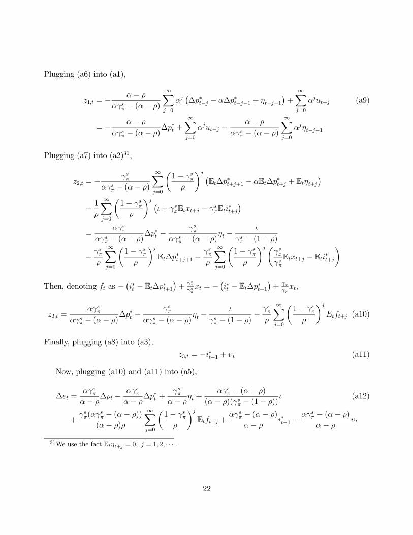
Plugging (a6) into (a1),
z1,t = −α− ρ
αγsπ − (α− ρ)
∞Xj=0
αj¡∆p∗t−j − α∆p∗t−j−1 + ηt−j−1
¢+
∞Xj=0
αjut−j (a9)
= − α− ρ
αγsπ − (α− ρ)∆p∗t +
∞Xj=0
αjut−j −α− ρ
αγsπ − (α− ρ)
∞Xj=0
αjηt−j−1
Plugging (a7) into (a2)31,
z2,t = −γsπ
αγsπ − (α− ρ)
∞Xj=0
µ1− γsπ
ρ
¶j ¡Et∆p∗t+j+1 − αEt∆p∗t+j + Etηt+j
¢− 1
ρ
∞Xj=0
µ1− γsπ
ρ
¶j ¡ι+ γsxEtxt+j − γsπEti∗t+j
¢=
αγsπαγsπ − (α− ρ)
∆p∗t −γsπ
αγsπ − (α− ρ)ηt −
ι
γsπ − (1− ρ)
− γsπρ
∞Xj=0
µ1− γsπ
ρ
¶j
Et∆p∗t+j+1 −γsπρ
∞Xj=0
µ1− γsπ
ρ
¶j µγsxγsπEtxt+j − Eti∗t+j
¶
Then, denoting ft as −¡i∗t − Et∆p∗t+1
¢+ γsx
γsπxt = −
¡i∗t − Et∆p∗t+1
¢+ γx
γπxt,
z2,t =αγsπ
αγsπ − (α− ρ)∆p∗t −
γsπαγsπ − (α− ρ)
ηt−ι
γsπ − (1− ρ)− γsπ
ρ
∞Xj=0
µ1− γsπ
ρ
¶j
Etft+j (a10)
Finally, plugging (a8) into (a3),
z3,t = −i∗t−1 + υt (a11)
Now, plugging (a10) and (a11) into (a5),
∆et =αγsπα− ρ
∆pt −αγsπα− ρ
∆p∗t +γsπ
α− ρηt +
αγsπ − (α− ρ)
(α− ρ)(γsπ − (1− ρ))ι (a12)
+γsπ(αγ
sπ − (α− ρ))
(α− ρ)ρ
∞Xj=0
µ1− γsπ
ρ
¶j
Etft+j +αγsπ − (α− ρ)
α− ρi∗t−1 −
αγsπ − (α− ρ)
α− ρυt
31We use the fact Etηt+j = 0, j = 1, 2, · · · .
22

Updating (a12) once and applying law of iterated expectations,
∆et+1 = ι+αγsπα− ρ
∆pt+1 −αγsπα− ρ
∆p∗t+1 +αγsπ − (α− ρ)
α− ρi∗t (a13)
+γsπ(αγ
sπ − (α− ρ))
(α− ρ)ρ
∞Xj=0
µ1− γsπ
ρ
¶j
Etft+j+1 + ωt+1,
where
ι =αγsπ − (α− ρ)
(α− ρ)(γsπ − (1− ρ))ι,
ωt+1 =γsπ(αγ
sπ − (α− ρ))
(α− ρ)ρ
∞Xj=0
µ1− γsπ
ρ
¶j
(Et+1ft+j+1 − Etft+j+1)
+γsπ
α− ρηt+1 −
αγsπ − (α− ρ)
α− ρυt+1,
and,
Etωt+1 = 0
23

B The Solution When α = ρ
When α equals ρ, we have the following system of difference equations.⎡⎢⎣ 1 −1 0
−γsπ 1 0
−γsπ 0 1
⎤⎥⎦⎡⎢⎣ Et∆pt+1
Et∆et+1
it
⎤⎥⎦ =⎡⎢⎣ ρ −ρ 0
0 0 ρ
0 0 ρ
⎤⎥⎦⎡⎢⎣ ∆pt
∆et
it−1
⎤⎥⎦+⎡⎢⎣ Et∆p∗t+1 − ρ∆p∗t + ηt
ι+ γsxxt − i∗tι+ γsxxt
⎤⎥⎦ , (b1)which can be represented by the following.
Etyt+1 = VΛV−1yt + ct, (b2)
where
V =
⎡⎢⎣ 0 1 1
1 1 1
1 1 0
⎤⎥⎦ , Λ =⎡⎢⎣ ρ 0 0
0 ρ1−γsπ
0
0 0 0
⎤⎥⎦ , V−1 =⎡⎢⎣ −1 1 0
1 −1 1
0 1 −1
⎤⎥⎦The system yields the same eigenvalues, α = ρ and ρ
1−(1−ρ)γπ. Therefore, when γπ is greater
than one, we have the saddle-path equilibrium as before. By pre-multiplying both sides of (b2)
by V−1, we get,
Etzt+1 = Λzt + ht, (b3)
where V−1yt = zt and V−1ct = ht.
We solve the system as follows.
z1,t =∞Xj=0
ρjh1,t−j−1 +∞Xj=0
ρjut−j (b4)
z2,t = −∞Xj=0
µ1− γsπ
ρ
¶j+1
Eth2,t+j (b5)
z3,t = h3,t−1 + υt, (b6)
where ut and υt are any martingale difference sequences.
Since yt = Vzt, ⎡⎢⎣ ∆pt
∆et
it−1
⎤⎥⎦ =⎡⎢⎣ 0 1 1
1 1 1
1 1 0
⎤⎥⎦⎡⎢⎣ z1,t
z2,t
z3,t
⎤⎥⎦ (b7)
24

Now, we find the analytical solutions for zt. Since ht = V−1ct,
ht =
⎡⎢⎣ −1 1 0
1 −1 1
0 1 −1
⎤⎥⎦⎡⎢⎣ (Et∆p∗t+1 − ρ∆p∗t + ηt) + ι+ γsxxt − i∗t
γsπ(Et∆p∗t+1 − ρ∆p∗t + ηt) + ι+ γsxxt − i∗tγsπ(Et∆p∗t+1 − ρ∆p∗t + ηt) + ι+ γsxxt − γsπi
∗t
⎤⎥⎦ ,thus,
h1,t = −(1− γsπ)¡Et∆p∗t+1 − ρ∆p∗t + ηt
¢(b8)
h2,t = Et∆p∗t+1 − ρ∆p∗t + ηt + ι+ γsxxt − γsπi∗t (b9)
h3,t = −(1− γsπ)i∗t (b10)
From (b4) and (b8),
z1,t = −(1− γsπ)∞Xj=0
ρj¡∆p∗t−j − ρ∆p∗t−j−1 + ηt−j−1
¢+
∞Xj=0
ρjut−j (b11)
= −(1− γsπ)∆p∗t +∞Xj=0
ρjut−j − (1− γsπ)∞Xj=0
ρjηt−j−1
From (b5) and (b9),
z2,t = −∞Xj=0
µ1− γsπ
ρ
¶j+1 ¡Et∆p∗t+j+1 − ρEt∆p∗t+j + Etηt+j + ι+ γsxEtxt+j − γsπEti∗t+j
¢(b12)
= (1− γsπ)∆p∗t −µ1− γsπ
ρ
¶ηt −
(1− γsπ)ι
ρ− (1− γsπ)
− γsπ
∞Xj=0
µ1− γsπ
ρ
¶j+1µEt∆p∗t+j+1 +
γsxγsπEtxt+j − Eti∗t+j
¶
Denoting ft as −¡i∗t − Et∆p∗t+1
¢+ γsx
γsπxt = −
¡i∗t − Et∆p∗t+1
¢+ γx
γπxt,
z2,t = (1− γsπ)∆p∗t − γsπ
∞Xj=0
µ1− γsπ
ρ
¶j+1
Etft+j −µ1− γsπ
ρ
¶ηt −
(1− γsπ)
ρ− (1− γsπ)ι (b13)
From (b6) and (b10),
z3,t = −(1− γsπ)i∗t−1 + υt (b14)
25

From (b7), (b13), and (b14),
∆pt = (1− γsπ)∆p∗t − γsπ
∞Xj=0
µ1− γsπ
ρ
¶j+1
Etft+j (b15)
−µ1− γsπ
ρ
¶ηt +
(1− γsπ)
(1− γsπ)− ρι− (1− γsπ)i
∗t−1 + υt
Updating (b15) once and applying the law of iterated expectations,
∆pt+1 = ι+ (1− γsπ)∆p∗t+1 − (1− γsπ)i∗t − γsπ
∞Xj=0
µ1− γsπ
ρ
¶j+1
Etft+j + ωt+1, (b16)
where
ι =(1− γsπ)
(1− γsπ)− ρι,
ωt+1 = −γsπ∞Xj=0
µ1− γsπ
ρ
¶j
(Et+1ft+j+1 − Etft+j+1)−µ1− γsπ
ρ
¶ηt+1 + υt+1,
and
Etωt+1 = 0
Note that there is no inertia for the domestic inflation in this solution, since there is no
backward looking component. Put it differently, when there is a shock, ∆pt+1 instantly jumps
to its long-run equilibrium.
On the contrary, ∆et+1 does have inertia. From (b7),
∆et = z1,t +∆pt (b17)
Plug (b11) into (b17) and update it once to get,
∆et+1 = ∆pt+1 − (1− γsπ)∆p∗t+1 +∞Xj=0
ρjut−j+1 − (1− γsπ)∞Xj=0
ρjηt−j, (b18)
where ∆pt+1 contains rational expectation of future fundamentals as defined in (b16). Note
that ∆et+1 exhibits inertia due to the presence of the martingale difference sequences.
In a nutshell, in the special case of ρ = α, domestic inflation instantly jumps to its long-run
equilibrium and all the convergence will be carried over by the exchange rate adjustments
26

Acknowledgement
Special thanks go to Lutz Kilian, Christian Murray, David Papell, Paul Evans, Eric Fisher,
and Henry Thompson for helpful suggestions. We also thank seminar participants at Bank of
Japan, Keio University, University of Houston, University of Michigan, Texas Tech University,
Auburn University, University of Southern Mississippi, the 2009 ASSA Meeting, the 72nd Mid-
west Economics Association Annual Meeting, the Midwest Macro Meeting 2008, and the 2009
NBER Summer Institute (EFSF).
27
References
Andrews, Donald W. K., “Exactly Median-Unbiased Estimation of First Order Autoregres-sive/Unit Root Models,” Econometrica, 1993, 61, 139—165.
and Hong-Yuan Chen, “Approximately Median-Unbiased Estimation of AutoregressiveModels,” Journal of Business and Economic Statistics, 1994, 12, 187—204.
Bils, Mark and Peter J. Klenow, “Some Evidence on the Importance of Sticky Prices,”Journal of Political Economy, 2005, 112, 947—985.
Boivin, Jean, “Has US Monetary Policy Changed? Evidence from Drifting Coefficients and
Real Time Data,” Journal of Money, Credit, and Banking, 2006, 38, 1149—1173.
Broda, Christian and David E. Weinstein, “Understanding International Price DifferencesUsing Barcode Data,” 2008. NBER Working Paper No. 14017.
Calvo, Guillermo, “Staggered Prices in a Utility Maximizing Framework,” Journal of Mon-etary Economics, 1983, 12, 383—398.
Carvalho, Carlos and Fernanda Nechio, “Aggregation and the PPP Puzzle in a Sticky-Price Model,” 2008. Manuscript.
Chen, Shiu-Sheng and Charles Engel, “Does ’Aggregation Bias’ Explain the PPP Puzzle?,”Pacific Economic Review, 2005, 10, 49—72.
Christiano, Lawrence J., Martin Eichenbaum, and Charles L. Evans, “Nominal Rigidi-ties and the Dynamic Effects of a Shock to Monetary Policy,” Journal of Political Economy,
2005, 113, 1—45.
Clarida, Richard and Daniel Waldman, “Is Bad News About Inflation Good News for theExchange Rate?,” 2007. NBER Working Paper No. 13010.
, Jordi Galí, and Mark Gertler, “Monetary Policy Rules in Practice: Some InternationalEvidence,” European Economic Review, 1998, 42, 1033—1067.
, , and , “Monetary Policy Rules and Macroeconomic Stability: Evidence and Some
Theory,” Quarterly Journal of Economics, 2000, 115, 147—180.
28

Crucini, Mario J. and Mototsugu Shintani, “Persistence in Law-of-One-Price Deviations:Evidence from Micro-Data,” Journal of Monetary Economics, 2008, 55, 629—644.
Efron, Bradley and Robert J. Tibshirani, An Introduction to the Bootstrap, London, UK:Chapman and Hall/CRC, 1993.
Eichenbaum, Martin and Jonas D.M. Fisher, “Estimating the Frequency of Price Re-optimization in Calvo-Style Models,” Journal of Monetary Economics, 2007, 54, 2032—2047.
Engel, Charles and Kenneth D. West, “Exchange Rates and Fundamentals,” Journal ofPolitical Economy, 2005, 113, 485—517.
and , “Taylor Rules and the Deutschmark-Dollar Exchange Rate,” Journal of Money,
Credit, and Banking, 2006, 38, 1175—1194.
Galí, Jordi and Mark Gertler, “Inflation Dynamics: A Structural Econometric Analysis,”Journal of Monetary Economics, 1999, 44, 195—222.
Hansen, Bruce E., “The Grid Bootstrap and the Autoregressive Model,” Review of Economicsand Statistics, 1999, 81, 594—607.
Hansen, Lars P., “Large Sample Properties of Generalized Method of Moments Estimators,”Econometrica, 1982, 50, 1029—1054.
and Thomas J. Sargent, “Formulating and Estimating Dynamic Linear Rational Expec-tations Models,” Journal of Economic Dynamics and Control, 1980, 2, 7—46.
and , “A Note on Wiener-Kolmogorov Prediction Formulas for Rational Expectations
Models,” 1981. Research Department Staff Report 69, Federal Reserve Bank of Minneapolis,
Minneapolis, MN.
and , “Instrumental Variables Procedures for Estimating Linear Rational Expectations
Models,” Journal of Monetary Economics, 1982, 9, 263—296.
Imbs, Jean, Haroon Mumtaz, Morten O. Ravn, and Helene Rey, “PPP Strikes Back:Aggregation and the Real Exchange Rates,” Quarterly Journal of Economics, 2005, 120,
1—43.
29

Kehoe, Patrick J. and Virgiliu Midrigan, “Stikcy Prices and Sectoral Real ExchangeRates.as,” 2007. Federal Reserve Bank of Minneapolis Working Paper 656.
Kilian, Lutz and Tao Zha, “Quantifying the Uncertainty about the Half-Life of Deviationsfrom PPP,” Journal of Applied Econometrics, 2002, 17, 107—125.
Kim, Hyeongwoo, “Essays on Exchange Rate Models under a Taylor Rule Type MonetaryPolicy,” 2006. Ph.D. Dissertation, Ohio State University.
, “A Note on Real Exchange Rate Dynamics and the Taylor Rule,” 2009. manuscript,
http://business.auburn.edu/ hzk0001/research.html.
Kim, Jaebeom, “Convergence Rates to PPP for Traded and Non-Traded Goods: A StructuralError Correction Model Approach,” Journal of Business and Economic Statistics, 2005, 23,
76—86.
and Masao Ogaki, “Purchasing Power Parity for Traded and Non-Traded Goods: AStructural Error Correction Model Approach,” Monetary and Economic Studies, 2004, 22,
1—26.
, , and Min-Seok Yang, “Structural Error Correction Models: A System Method for
Linear Rational Expectations Models and an Application to an Exchange Rate Model,”
Journal of Money, Credit, and Banking, 2007, 39, 2057—2075.
Kleibergen, Frank and Sophocles Mavroeidis, “Inference on Subsets of Parameters inGMM without Assuming Identification,” Journal of Business and Economic Statistics, 2009,
forthcoming.
Magnusson, Leandro M. and Sophocles Mavroeidis, “Identification-Robust MinimumDistance Estimation of the New Keynesian Phillips Curve,” 2009. manuscript.
Mark, Nelson C., International Macroeconomics and Finance: Theory and EconometricMethods, Oxford, UK: Blackwell Publishers, 2001.
, “Changing Monetary Policy Rules, Learning, and Real Exchange Rate Dynamics,” 2005.
National Bureau of Economic Research Working Paper No. 11061.
30

Molodtsova, Tanya, Alex Nikolsko-Rzhevskyy, and David H. Papell, “Taylor Rulewith Real-Time Data: A Tale of Two Countries and One Exchange Rate,” Journal of Mon-
etary Economics, 2008, 55, S63—S79.
and David H. Papell, “Out-of-Sample Exchange Rate Predictability with Taylor RuleFundamentals,” 2007. Manuscript, University of Houston.
Murray, Christian J. and David H. Papell, “The Purchasing Power Parity PersistenceParadigm,” Journal of International Economics, 2002, 56, 1—19.
and , “Do Panels Help Solve the Purchasing Power Parity Puzzle?,” Journal of Business
and Economic Statistics, 2005, 23, 410—415.
Mussa, Michael, “AModel of Exchange Rate Dynamics,” Journal of Political Economy, 1982,90, 74—104.
Nakamura, Emi and Jón Steinsson, “Five Facts About Prices: A Reevaluation of MenuCost Models,” Quarterly Journal of Economics, 2008, 123, 1415—1464.
Negro, Marco Del and Frank Schorfheide, “Forming Priors for DSGE Models (and HowIt Affects the Assessment of Nominal Rrigidities),” Journal of Monetary Economics, 2008,
55, 1191—1208.
Ng, Serena and Pierre Perron, “Lag Length Selection and the Construction of Unit RootTests with Good Size and Power,” Econometrica, 2001, 69, 1519—1554.
Ogaki, Masao, “Generalized Method of Moments: Econometric Applications,” in G. S. Mad-dala, C. R. Rao, and H. D. Vinod, eds., Handbook of Statistics, Vol.II, North-Holland Ams-
terdam 1993, pp. 455—488.
Parsley, David C. and Shang-Jin Wei, “A Prism into the PPP Puzzles: The Micro-
Foundations of Big Mac Real Exchange Rates,” Economic Journal, 2007, 117, 1336—1356.
Rogoff, Kenneth, “The Purchasing Power Parity Puzzle,” Journal of Economic Literature,1996, 34, 647—668.
Rossi, Barbara, “Confidence Intervals for Half-Life Deviations From Purchasing Power Par-
ity,” Journal of Business and Economic Statistics, 2005, 23, 432—442.
31

Sargent, Thomas J., Macroeconomic Theory, second ed., New York: Academic Press, 1987.
Sbordone, Argia M., “Prices and Unit Labor Costs: A New Test of Price Stickiness,” Journalof Monetary Economics, 2002, 49, 265—292.
, “Do Expected Future Marginal Costs Drive Inflation Dynamics?,” Journal of Monetary
Economics, 2005, 52, 1183—1197.
Smets, Frank and Rafael Wouters, “Shocks and Frictions in U.S. Business Cycles: ABayesian DSGE Approach,” American Economic Review, 2007, 97, 586—606.
Steinsson, Jón, “The Dynamic Behavior of the Real Exchange Rate in Sticky-Price Models,”American Economic Review, 2008, 98, 519—533.
Stock, James H. and Mark W. Watson, “A Simple Estimator of Cointegrating Vectors inHigher Order Integrated Systems,” Econometrica, 1993, 61, 783—820.
Svensson, Lars E.O., “Open-Economy Inflation Targeting,” Journal of International Eco-nomics, 2000, 50, 155—183.
West, Kenneth D., “A Specification Test for Speculative Bubbles,” Quarterly Journal of
Economics, 1987, 12, 553—580.
, “Estimation of Linear Rational Expectations Models, In the Presence of Deterministic
Terms,” Journal of Monetary Economics, 1989, 24, 437—442.
Woodford, Michael, “How Important Is Money in the Conduct of Monetary Policy,” Journalof Money, Credit, and Banking, 2007, forthcoming.
32

Table 1. GMM Estimation of the US Taylor Rule Estimation
Deviation Sample Period γπ (s.e.) γx (s.e.) ρ (s.e.)Real GDP 1959:Q1-2003:Q4 1.466 (0.190) 0.161 (0.054) 0.820 (0.029)
1959:Q1-1979:Q2 0.605 (0.099) 0.577 (0.183) 0.708 (0.056)1979:Q3-2003:Q4 2.517 (0.306) 0.089 (0.218) 0.806 (0.034)
Unemployment 1959:Q1-2003:Q4 1.507 (0.217) 0.330 (0.079) 0.847 (0.028)1959:Q1-1979:Q2 0.880 (0.096) 0.217 (0.072) 0.710 (0.057)1979:Q3-2003:Q4 2.435 (0.250) 0.162 (0.078) 0.796 (0.034)
Notes: i) Inflations are quarterly changes in log CPI level (ln pt− ln pt−1). ii) Quadraticallydetrended gaps are used for real GDP output deviations. iii) Unemployment gaps are 5 yearbackward moving average unemployment rates minus current unemployment rates. iv) The setof instruments includes four lags of federal funds rate, inflation, output deviation, long-shortinterest rate spread, commodity price inflation, and M2 growth rate.
33

Table 2. GMM Median Unbiased Estimates and 95% Grid-t Confidence Intervals
Country αGMM CIgrid-t HL HL CIgrid-t J (pv)Australia 0.884 [0.837,0.943] 1.404 [0.977,2.953] 5.532 (0.700)Austria 0.804 [0.786,0.826] 0.793 [0.721,0.904] 8.173 (0.417)Belgium 0.816 [0.794,0.844] 0.852 [0.751,1.019] 7.942 (0.439)Canada 1.000 [0.967,1.000] ∞ [5.109, ∞ ) 4.230 (0.836)Denmark 0.937 [0.874,1.000] 2.675 [1.290, ∞ ) 6.272 (0.617)Finland 0.948 [0.897,1.000] 3.235 [1.587, ∞ ) 7.460 (0.488)France 0.799 [0.777,0.822] 0.772 [0.688,0.885] 8.517 (0.385)Germany 0.786 [0.767,0.809] 0.721 [0.652,0.819] 9.582 (0.296)Italy 0.832 [0.806,0.864] 0.945 [0.805,1.181] 4.228 (0.836)Japan 0.754 [0.729,0.782] 0.613 [0.549,0.706] 9.800 (0.279)Netherlands 0.838 [0.798,0.883] 0.984 [0.766,1.388] 6.638 (0.576)New Zealand 0.805 [0.786,0.828] 0.799 [0.718,0.918] 6.874 (0.550)Norway 0.873 [0.785,0.971] 1.271 [0.716,5.983] 8.225 (0.412)Portugal 0.792 [0.779,0.806] 0.741 [0.694,0.803] 6.132 (0.633)Spain 0.896 [0.856,0.943] 1.581 [1.114,2.954] 6.738 (0.565)Sweden 1.000 [0.945,1.000] ∞ [3.088, ∞ ) 7.107 (0.525)Switzerland 0.831 [0.795,0.870] 0.937 [0.755,1.240] 9.136 (0.331)UK 0.778 [0.756,0.806] 0.690 [0.620,0.801] 17.49 (0.025)Median 0.832 [0.795,0.867] 0.941 [0.753,1.211] -
Notes: i) The US$ is the base currency. ii) Unemployment gaps are used for output deviations.iii) Sample periods are 1979.II-1998.IV (78 observations) for Eurozone countries and are 1979.II-2003.IV (98 observations) for non-Eurozone countries. iv) CIgrid-t denotes the 95% confidenceintervals that were obtained by 500 residual-based bootstrap replications on 30 grid points(Hansen, 1999). v) J denotes the J-statistic and pv is its associated p-values.
34

Table 3. Univariate Median Unbiased Estimates and Grid-t Confidence Intervals
Country αLS CIgrid-t HL HL CIgrid-tAustralia 0.972 [0.891,1.000] 6.173 [1.494, ∞ )Austria 0.945 [0.866,1.000] 3.087 [1.205, ∞ )Belgium 0.924 [0.847,1.000] 2.203 [1.045, ∞ )Canada 1.000 [0.946,1.000] ∞ [3.122, ∞ )Denmark 0.942 [0.866,1.000] 2.886 [1.200, ∞ )Finland 0.959 [0.883,1.000] 4.107 [1.390, ∞ )France 0.931 [0.847,1.000] 2.432 [1.044, ∞ )Germany 0.950 [0.852,1.000] 3.349 [1.078, ∞ )Italy 0.943 [0.859,1.000] 2.932 [1.138, ∞ )Japan 0.952 [0.886,1.000] 3.511 [1.428, ∞ )Netherlands 0.936 [0.839,1.000] 2.619 [0.990, ∞ )New Zealand 0.959 [0.923,0.997] 4.089 [2.174,61.29]Norway 0.934 [0.851,1.000] 2.529 [1.073, ∞ )Portugal 0.975 [0.913,1.000] 6.765 [1.904, ∞ )Spain 0.959 [0.898,1.000] 4.129 [1.604, ∞ )Sweden 0.959 [0.891,1.000] 4.089 [1.497, ∞ )Switzerland 0.951 [0.862,1.000] 3.481 [1.168, ∞ )UK 0.932 [0.845,1.000] 2.442 [1.028, ∞ )Median 0.951 [0.866,1.000] 3.415 [1.203, ∞ )
Notes: i) The US$ is the base currency. ii) Sample periods are 1979.II-1998.IV (78 observations)for Eurozone countries and are 1979.II-2003.IV (98 observations) for non-Eurozone countries. iii)CIgrid-t denotes the 95% confidence intervals that were obtained by 500 residual-based bootstrapreplications on 30 grid points (Hansen, 1999).
35

Table 4. Univariate Median Unbiased Half-Life Estimates: AR(1) vs. AR(p)
Country pMAIC pMBIC HLAR(1) HLIRFAustralia 1 1 6.173 6.173Austria 1 1 3.087 3.087Belgium 4 1 2.203 2.884Canada 6 1 ∞ ∞Denmark 4 1 2.886 3.883Finland 6 2 4.107 3.631France 1 1 2.432 2.432
Germany 6 1 3.349 3.386Italy 3 1 2.932 ∞Japan 1 1 3.511 3.511
Netherlands 6 1 2.619 2.882New Zealand 9 1 4.089 3.895
Norway 1 1 2.529 2.529Portugal 6 1 6.765 ∞Spain 2 1 4.129 12.13
Sweden 4 4 4.089 3.387Switzerland 1 1 3.481 3.481
UK 3 1 2.442 3.129Median 3.5 1 3.415 3.496
Notes: i) pMAIC and pMBIC denote the lag length chosen by the modified Akaike Informationcriteria and the modified Bayesian Information criteria (Ng and Perron, 2001) with maximum12 lags, respectively. ii) HLAR(1) refers the half-life point estimates with an AR(1) specificationand was replicated from Table 3 for a comparison purpose. iii) HLIRF deontes the half-life pointestimates obtained from the impulse-response function with the lag length chosen by pMAIC.HLIRF with pMBIC is not reported because the estimates are virtually the same as HLAR(1). iv)We correct the median bias of each autoregressive coefficient for higher order AR(p) conditioningon all other coefficients.
36