lecture notes 5 purchasing power parity - american … · lecture notes 5 purchasing power parity...

Lecture Notes 5

Purchasing Power Parity

International Economics: Finance Professor: Alan G. Isaac

5 Purchasing Power Parity 1

5.1 Commodity Price Parity . . . . . . . . . . . . . . . . . . . . . . . . . . . . . 2

5.1.1 Barriers to Commodity Arbitrage . . . . . . . . . . . . . . . . . . . . 4

5.2 Purchasing Power . . . . . . . . . . . . . . . . . . . . . . . . . . . . . . . . . 7

5.2.1 Price Indices . . . . . . . . . . . . . . . . . . . . . . . . . . . . . . . . 8

5.3 Absolute Purchasing Power Parity . . . . . . . . . . . . . . . . . . . . . . . . 9

5.3.1 The Big Mac Standard . . . . . . . . . . . . . . . . . . . . . . . . . . 10

5.3.2 Explaining the Deviations . . . . . . . . . . . . . . . . . . . . . . . . 12

5.3.3 Commodity Price Parity . . . . . . . . . . . . . . . . . . . . . . . . . 13

5.4 Real Exchange Rates and Purchasing Power . . . . . . . . . . . . . . . . . . 14

5.5 The Purchasing Power Parity Doctrine . . . . . . . . . . . . . . . . . . . . . 15

5.6 Policy Applications . . . . . . . . . . . . . . . . . . . . . . . . . . . . . . . . 16

5.6.1 Setting Parities . . . . . . . . . . . . . . . . . . . . . . . . . . . . . . 16

5.6.2 Comparing Real Incomes . . . . . . . . . . . . . . . . . . . . . . . . . 17

1

5.6.3 Choice of Price Index . . . . . . . . . . . . . . . . . . . . . . . . . . . 19

5.7 Expected Purchasing Power Parity . . . . . . . . . . . . . . . . . . . . . . . 21

5.8 Long-Run Purchasing Power Parity . . . . . . . . . . . . . . . . . . . . . . . 22

5.8.1 The Balassa-Samuelson Critique . . . . . . . . . . . . . . . . . . . . . 23

5.8.2 The Houthakker-Magee Critique . . . . . . . . . . . . . . . . . . . . . 26

5.9 Testing Purchasing Power Parity . . . . . . . . . . . . . . . . . . . . . . . . 27

5.9.1 Regression Tests of PPP . . . . . . . . . . . . . . . . . . . . . . . . . 29

5.9.2 Long-Run Purchasing Power Parity . . . . . . . . . . . . . . . . . . . 30

5.9.3 Regression Tests of Long-Run PPP . . . . . . . . . . . . . . . . . . . 31

5.9.4 Some Studies . . . . . . . . . . . . . . . . . . . . . . . . . . . . . . . 34

Terms and Concepts . . . . . . . . . . . . . . . . . . . . . . . . . . . . . . . 35

Problems for Review . . . . . . . . . . . . . . . . . . . . . . . . . . . . . . . 35

Bibliography 39

Bibliography 51

2 LECTURE NOTES 5. PURCHASING POWER PARITY

A key ingredient of the monetary approach is the assumption that the real exchange

rate (Q) is exogenous. This exogeneity assumption allows us to view (5.1) as determining a

relationship between exchange rates and relative price levels.

S = QP

P ∗ (5.1)

In this chapter we explore the underpinnings of (5.1) and consider some empirical tests.

Learning Goals

After reading this chapter, you will understand:

� the real exchange rate and its relationship to purchasing power parity.

� ways in which supply and demand influence the real exchange rate even in the longrun.

� the relationship between commodity price parity and purchasing power parity.

� how prices and exchange rates are related in the long run.

5.1 Commodity Price Parity

If spatial arbitrage were costless for all commodities, where you live would have no effect

on the purchasing power of your income. Recall that arbitrage is the simultaneous purchase

of something where it is cheap and sale of it where it is dear. In chapter 2, we discussed

how spatial arbitrage ensures that exchange rates are essentially identical in geographically

dispersed markets. Similarly, when it is not costly to spatially arbitrage a commodity, that

commodity should be equally affordable in geographically dispersed markets. For example,

we do not expect that changing U.S. dollars into euros and then buying gold in Paris will

get us more gold than simply buying it in the U.S.

Let us begin by considering an extreme case. Imagine a good that is truly costless to

transport. Domestically this means that it must sell for the same price at every location.

That is, the law of one price must hold for this good. This must also be true internationally.

If the good is entirely costless to transport, and if there are no barriers to international trade

©2015 Alan G. Isaac

5.1. COMMODITY PRICE PARITY 3

in the good, then it must be equally costly to acquire at every location. This implies a link

between the price of the good in different currencies and the exchange rates between those

currencies.

If this costlessly arbitraged good can be bought and sold for Pi domestically and P ∗i

abroad, then we must know the exchange rate as well. For unless

Pi = SP ∗i (5.2)

there will be an opportunity for profitable arbitrage. For example, when Pi < SP ∗i , an

arbitrageur can buy the good domestically for Pi, sell it abroad for P ∗i , and sell the foreign

currency for SP ∗. Such spatial arbitrage would add to demand where the good is cheap and

to supply where the good is dear. Such arbitrage activity should continue until the equality

(5.2) holds. Spatial arbitrage ensures that commodities the law of one price. Equation (5.2)

says this is true even across international boundaries, when different currency denominations

are involved. Equation (5.2) is known as commodity price parity (CPP). Commodity price

parity is just the law of one price applied internationally.

If commodity price parity applied to all commodities, a given income would buy the

same goods in any location. In this sense, a consumer’s country of residence would not

affect her consumption opportunities. Changes in exchange rates would not imply changes

in consumption possibilities. So we can see that under universal CPP, consumers face no

exchange rate risk.1

Example:On 12 October 2009, one ounce of gold sold in New York for USD 1056 and sold in Londonfor GBP 669. One GBP sold in both locations for about USD 1.58. Gold satisfies CPP,since 1056 ≈ 1.58 ∗ 669.

1To eliminate exchange rate risk for the owners of factors of production, in addition to CPP we need allinputs (including labor) to be spatially arbitraged.



CPP Example

-----------

On 30 September 2010

- 1oz of gold sold in New York for USD 1307

- 1 oz also sold in London for GBP 830.

- One GBP sold in both locations for about USD 1.575.

Gold satisfies CPP: 1307 = 1.575 * 830

CPP Example (cont.)

---------------------

On 17 October 2011

- 1oz of gold sold in New York for USD 1783.00

- 1 oz also sold in London for GBP 1069.326

- One GBP sold in both locations for about USD 1.5795.

Gold satisfies CPP: 1689 = 1.5795 * 1069.326

CPP Example (cont.)

---------------------

On 22 February 2012

- 1oz of gold sold in New York for USD 1780

- 1 oz also sold in London for GBP 1135.820

- One GBP sold in both locations for about USD 1.56715

Gold satisfies CPP: 1135.820 = 1780.00 / 1.56715

5.1.1 Barriers to Commodity Arbitrage

Even within a single country, arbitrage activity is not costless, so the law of one price

never holds exactly.2 Transportation costs and restraints of trade will mean that the costs of

delivering a commodity will differ at different geographical locations. These cost differentials

will influence pricing, and therefore transportation costs and restraints of trade are two likely

sources of deviations from the law of one price. This is even more important internationally:

transportation costs and restraints of trade can lead to substantial deviation from CPP.

2See O’Connell and Wei (2002) for evidence on the tendency toward satisfaction of the law of one pricein the United States.


5.1. COMMODITY PRICE PARITY 5

Transportation Costs

Transportation costs are a natural barrier to trade. Large countries and countries with

poorly developed transportation infrastructure may experience large deviations in prices

across spatial locations. Even in the presence of transportation costs, such as shipping and

insurance fees, arbitrage limits the divergence of prices. The prices can differ by as much

as the transportation costs without consequence, but when the price difference exceeds the

transportation costs, incentives arise for arbitrage activity.

When we are comparing foreign and domestic prices, we must of course measure them

in the same currency. For example, when the U.S. dollar roughly doubled in value against

the German mark in the early 1980s, without corresponding movements in U.S. and German

automobile prices, people began to buy automobiles in Germany and ship them to the

U.S. However the extend of such arbitrage was modest, and it failed to eliminate the price

differential.3

Some goods and services are subject to extremely high transportation costs relative to

their value. Consider trying to transport haircuts or housing services over any significant

distance.4 Even large international price discrepancies will not offset the transactions costs

required for arbitrage. These goods are considered to be non-traded.

Non-Traded Inputs

Some non-traded goods are inputs into the production of other goods. In addition, some fac-

tors of production are not cheaply transportable across locations. This means that the costs

of inputs into the production of traded goods will diverge between geographical locations,

even within a country. (Land in New York city is going to be costly.)

It does not follow that prices of traded goods will also differ. If the traded goods are

easily arbitraged, price differences at different locations will be limited. This may affect the

3See Caves, Frankel, and Jones (1996, p.429) for additional discussion.4Haircuts are a traditional example of a non-traded good, but in 2002 a student told me that some

Austrians were crossing into the Czech Republic to visit (much cheaper) hair stylists.



profitability of producing goods at different locations, when input costs vary geographically.

Restraints of Trade

There are many different kinds of trade restraints that affect the arbitrage of goods and ser-

vices. Anything institution that retards the spatial arbitrage of commodities may be viewed

as a restraint on trade. Within a country this includes prohibitions on the provision of profes-

sional services across regional boundaries (as in the state-specific licensing of lawyers in the

U.S.) as well as laws designed to allow differing regional rates of commodity taxation. Inter-

national trade barriers include quotas, import tariffs, and export duties: when successfully

enforced, these allow domestic and foreign prices to diverge. As with transportation costs,

tariffs create a band of possible divergence between the domestic and foreign prices.5 In the

extreme case, when trade barriers or transportation costs are prohibitively high, the band

of possible divergence becomes so wide that geographical arbitrage never takes place. Once

again, such commodities will be non-traded, and large divergences between the domestic and

foreign prices may arise.6 Successfully enforced quotas prevent arbitrage of more than a fixed

quantity, again allowing large international price differentials. Agricultural products are a

classic example of goods whose arbitrage is prevented by high tariff barriers.

Some laws are specifically designed to limit entry or to segment markets. Just as these

can prevent arbitrage within a country, they can prevent international arbitrage. Licensing

laws are an example. For example, foreign lawyers cannot provide domestic legal services

unless they acquire domestic credentials. When domestic and foreign markets are segmented,

so that a firm faces differing degrees of market power in different markets, a firm may price

its product differently at home and abroad.

5See Samuelson (1964).6In principle, even the prices of non-traded goods can show some tendency to equality, since they may

be substitutes for traded goods in consumption and may be produced with common or closely substitutablefactors of production.


5.2. PURCHASING POWER 7

Imperfect Competition

When a firm produces a commodity for which there are no close substitutes, it can exercise

market power. Although it can affect the price of its product, this in itself does not mean

that it can cause deviations from CPP. In order to price the product differently in different

geographical locations, the firm must not face arbitrage activity that would move the good

from low price locations to high price locations. Therefore transportation costs and barriers

to trade will remain the key determinants of deviations from CPP, even in the presence of

market power.

For example, in the mid-1990s New Zealand decided to permit parallel imports. A

“parallel import” occurs when an imported good is legally purchased in one country and

then imported into another market. Parallel imports are a method of circumventing the

exporters intended distribution channels. New Zealand’s new policy allowed importers to

bring in brand name goods for which they did not have a franchise, thus undermining the

ability purveyors of these goods to segment markets in order to maintain high prices. At

the time, the United States Trade Representative voiced strong opposition to this move,

taking the stance that parallel imports facilitate piracy and complicate the enforcement of

intellectual property rights.

5.2 Purchasing Power

When commodity price parity fails, the consumer’s geographical location affects her pur-

chasing power. When we speak of ‘purchasing power’ we refer to control over a collection of

commodities (rather than over a single commodity). We generally assess purchasing power

by constructing a price index based on, say, a typical consumption basket. For example,

we may determine the purchasing power of nominal personal income by deflating by the

consumer price index (CPI ).



5.2.1 Price Indices

What is the real “purchasing power” of a given nominal income? If you were a consumer of

only a single good, there would be a simple answer to this question: you could deflate the

nominal income by dividing it by the price of that good, thereby determining the number

of units of the good your income will buy. However, consumers purchase many goods.

Economists answer the purchasing-power question by constructing a price index, which they

use to deflate nominal income. You can very roughly think of the price index as the domestic

currency cost of a basket of commodities, so that purchasing power of a given nominal income

is measured as the number of these baskets that income can purchase.

Suppose we construct a price index based on a basket of n commodities.

CPI = f(P1, . . . , Pn) (5.3)

We expect all price indices to share certain properties. For example, if the price of any

commodity in the basket increases, the price index should increase. We call this property

monotonicity. A very important property such a price index should have is that when every

commodity in the basket doubles in price, then the price index should double. Similarly, if all

prices are cut in half, the price index should be halved. We call this property homogeneity.7

Homogeneity means that equiproportional movements in all prices lead to a proportional

movement in the price index. Given CPP, so that Pi = SP ∗i holds for every commodity in

the basket, homogeneity implies that we can write

CPIdef= f(P1, . . . , Pn)

CPP= f(SP ∗

1 , . . . , SP∗n)

hom= Sf(P ∗

1 , . . . , P∗n)

(5.4)

7More precisely, the price index is homogeneous of degree one in the commodity prices. A good consumerprice index should also be concave, representing the ability of consumers to substitute among commodities,but not all price indices satisfy concavity.


5.3. ABSOLUTE PURCHASING POWER PARITY 9

Now if we construct the foreign price index in the identical fashion as the domestic price

index, so that

CPI ∗ = f(P ∗1 , . . . , P

∗n) (5.5)

Then we have a relationship that looks very much like CPP:

CPI = S CPI ∗ (5.6)

We call this relationship absolute purchasing power parity. Absolute purchasing power

parity says that countries have equal price levels when expressed in a common currency.

Equivalently, absolute purchasing power parity implies that the spot rate equals the relative

price level.

S = CPI /CPI ∗ (5.7)

5.3 Absolute Purchasing Power Parity

The idea that exchange rates should be linked to national price levels has a long history

(Einzig, 1970). The classic statement, however, was given by Cassel (1918, p.413).

The general inflation which has taken place during the war has lowered this

purchasing power in all countries, though in a very different degree, and the rates

of exchanges should accordingly be expected to deviate from their old parity in

proportion to the inflation of each country.

At every moment the real parity between two countries is represented by this

quotient between the purchasing power of the money in the one country and

the other. I propose to call this parity “the purchasing power parity.” As long

as anything like free movement of merchandise and a somewhat comprehensive

trade between the two countries takes place, the actual rate of exchange cannot

deviate very much from this purchasing power parity.



Cassel is suggesting that the spot rate between two currencies should equal the relative

price level between the two countries, a proposition we have called absolute purchasing power

parity.8 We have seen that absolute PPP is implied when foreign and domestic price indices

are identically constructed and commodity price parity holds for all commodities in the

“market basket” on which the price indices are based. These are very restrictive conditions.

For many commodities, commodity price parity does not hold. In addition, price index

construction differs widely among countries.

The Penn World Table (PWT) constructs price indices based on a common market basket

of about 150 commodities (Summers and Heston, 1991), which should address the first

of these concerns. Nevertheless, as seen in the second column of table 5.1, considerable

deviations from purchasing power parity are evident.

5.3.1 The Big Mac Standard

Since 1986, The Economist has published yearly international price comparisons for McDon-

ald’s “Big Mac” sandwich. The composition of the Big Mac is generally uniform, making

it an internationally comparable “basket of commodities” that is an attractive candidate

for PPP comparisons. In addition, most of the ingredients of the Big Mac are individually

traded as standardized commodities on international markets. For such commodities, we

expect the law of one price to hold at least approximately. However Pakko and Pollard

(1996) show that relative Big Mac prices are highly correlated with the PWT measure. This

is illustrated by in table 5.1.

While table 5.1 gives little evidence of absolute PPP, Pakko and Pollard find somewhat

more support for long-run relative PPP. However the Big Mac time series is very short, so

it is difficult to assess the long-run evidence.

8As noted by Isard (1995, p.58), Cassel later allowed for short-run deviations from PPP.



A B C

United States 3.06 -- --

Argentina 1.64 1.55 -46

Australia 2.50 1.06 -18

Brazil 2.39 1.93 -22

Britain 3.44 1.63(*) +12

Canada 2.63 1.07 -14

Chile 2.53 490 -17

China 1.27 3.43 -59

Czech Republic 2.30 18.4 -25

Denmark 4.58 9.07 +50

Egypt 1.55 2.94 -49

Euro area 3.58 1.05(*) +17

Hong Kong 1.54 3.92 -50

Hungary 2.60 173 -15

Indonesia 1.53 4,771 -50

Japan 2.34 81.7 -23

Malaysia 1.38 1.72 -55

Mexico 2.58 9.15 -16

New Zealand 3.17 1.45 +4

Peru 2.76 2.94 -10

Philippines 1.47 26.1 -52

Poland 1.96 2.12 -36

Russia 1.48 13.7 -52

Singapore 2.17 1.18 -29

South Africa 2.10 4.56 -31

South Korea 2.49 817 -19

Sweden 4.17 10.1 +36

Switzerland 5.05 2.06 +65

Taiwan 2.41 24.5 -21

Thailand 1.48 19.6 -52

Turkey 2.92 1.31 -5

Venezuela 2.13 1,830 -30

Figure 5.1: Big Mac Standard

According to the table, the euro is overvalued against the dollar by 17%. Tocompute this overvaluation, you need more information than is directly in thetable. At the time, a Big Mac cost around EUR 2.92 in the euro zone andUSD 3.06 in the U.S. We therefore compute the CPP exchange rate as aboutEUR-USD 1.05 (=3.06/2.92). The exchange rate at the time was EUR-USD1.225, so the Big Mac standard says that percentage overvaluation is about17% (=(1.225-1.05)/1.05).Source: Economist Magazine 2005-06-09, http://www.economist.com/

markets/bigmac/

Legend for chart:A: Dollar price of Big Mac price at current exchange rate: SP ∗.B: Implied PPP value of the dollar (USD base currency, except for pound andeuro): P/P ∗.C: Under (-)/over (+) valuation against the dollar(*) USD is quote currency.Notes: U.S. Big Mac price is an average of New York, Chicago, San Fran-cisco and Atlanta prices. EU Big Mac price is a weighted average of membercountries.



Country P/SPUS (PWT) P/SPUS (Big Mac)Australia 0.98 0.86Belgium 1.13 1.29Britain 1.10 1.32Canada 1.04 0.90Denmark 1.40 1.85France 1.19 1.42Germany 1.27 1.14Hong Kong 0.75 0.51Ireland 1.06 1.00Italy 1.22 1.29Japan 1.41 1.25Netherlands 1.14 1.24Singapore 0.91 0.70Spain 1.08 1.50Sweden 1.51 1.91Source: Pakko and Pollard (1996, p.5)

Table 5.1: PPP Indicators (1991)

5.3.2 Explaining the Deviations

We have seen that there are two basic sources of deviation from absolute PPP: deviations

from CPP (trade barriers, including transportation costs), and differences in the construction

of domestic and foreign price indices. By focusing on the Big Mac, we have tried to limit

the relevance of the composition of the price index. (We will return to this.) Further,

transportation costs do not immediately suggest themselves as an explanation of the Big

Mac parity deviations, for as noted above the Big Mac ingredients are internationally traded

standardized commodities. However it is a mistake to identify brand name products with

their ingredients: what is being sold is really the product bundled with a reputation. If

the Big Mac has no close substitutes, the ability to trade the ingredients may not offset the

difficulty in transporting the final product. McDonald’s may be able to “price to market”

because of the lack of competition in some markets. Such explanations based on imperfect

competition have gained in popularity. For example, Feenstra and Kendall (1994) find

significant PPP deviations trace to the incomplete pass-through of exchange rate changes



into final goods prices. Finally, as pointed out by O’Connell and Wei (2002), franchise

restaurant meal have a significant input of nontraded intermediate inputs. Indeed, citetong-

1997-jimf estimates that non-traded goods constitute 94% of the prices of a Big Mac.

5.3.3 Commodity Price Parity

Isard (1977) examines the law of one price using wholesale and export price data on relatively

disaggregated groups of manufactured goods. He looks at the U.S., Japan, and Germany for

1970–1975. Perhaps surprisingly, even at his level of disaggregation the law of one price fails,

and nominal exchange rate changes affect relative prices. Kravis et al. (1978a) disaggregate

even further and obtain similar results. The finding that nominal exchange rate changes

affect disaggregated relative prices for traded goods should make us pessimistic about PPP

for aggregate price indices. And indeed, the correlation between real and nominal exchange

rates is extremely strong.

Further, the ingredients may be subject to legal restrictions on trade. For example, most

countries restrict agricultural imports with tariffs and quotas. Pakko and Pollard point

out that Korea looks consistently overvalued on the Big Mac standard, and it maintains

high barriers against beef imports. Such import restrictions will tend to raise prices in the

importing country, making its currency look overvalued. Similarly, differing tax practices

are another possible source of deviation: the Big Mac prices reported by The Economist

are inclusive of taxes. Countries with higher taxes will therefore appear to have overvalued

currencies. Pakko and Pollard give an example of this effect: when Canada imposed its

national seven percent sales tax in 1992, the price of a Big Mac rose by about the same

percentage.



5.4 Real Exchange Rates and Purchasing Power

In an ordinary year you exchange domestic money for goods, and as a result your annual

expenditures are naturally measured in units of the national currency. If you spend a year

abroad, you use foreign money to make your daily purchases. In this case your annual

expenditures are naturally measured in units of that national currency. How might we

compare your expenditures at home and abroad?

We might simply take your foreign expenditures and multiply them by the exchange rate,

S, in order to find out the domestic currency value of your spending. However, this proce-

dure will not tell us much about your standard of living while you were abroad. Although

individuals must make monetary exchanges, their central concern is their control over goods

and services. It would be nice to have a simple way to represent the material standard of

living that your expenditures in each country represent. For this, we need a way to transform

your nominal expenditures (measured in currency units) into real expenditures. While there

is no perfect way to do this, economists generally turn nominal into real expenditures by

deflating nominal expenditures with a consumer price index.

We will make our first approach to the real exchange rate in a very special setting.

Suppose you are considering spending a year abroad. Let’s construct your domestic consumer

price index P as the cost in domestic currency of your current consumption basket. Let us

then construct your foreign consumer price index P ∗ as the cost abroad (in foreign currency)

you would have to incur to be just as happy as you would be with your current consumption

basket. So each price index is simply the monetary cost of a specific consumption basket.

While the consumption basket is different in each country, you would be equally happy with

either basket.

Suppose you are a U.S. student considering a year abroad, and that you have USD 15k

for living expenses. In the U.S., this will afford you a material standard of living of USD

15k/P . If you spend the year abroad, you will have USD 15k/S in foreign currency to spend.

Of course you are likely to buy different things abroad than at home: these things constitute


5.5. THE PURCHASING POWER PARITY DOCTRINE 15

your foreign consumption basket. Your material standard of living abroad will therefore be

(USD 15k/S)/P ∗. Your relative material standard of living, Q, is therefore given by (5.8).

Q =SP ∗

P(5.8)

This is just the ratio of your material standard of living at home to your material standard

of living abroad. If Q rises, it becomes more of a sacrifice for you to live abroad.

5.5 The Purchasing Power Parity Doctrine

The relationship (5.6) between domestic and foreign price levels is known as absolute PPP.

It should be clear that absolute PPP depends on very special circumstances: we arrived

at (5.6) by assuming CPP (for every commodity) and that the domestic and foreign price

indices were constructed identically. Since both of these assumptions seriously misrepresent

the relationship between the price indices of different nations, we cannot expect absolute

PPP to hold between actual price indices.

However the real exchange rate may nevertheless be stable. Recall our definition of the

real exchange rate from chapter 3.

Q = SP ∗

P(5.9)

The purchasing power parity doctrine holds that, in the long run, Q is a constant determined

by real economic activity (along with any trade barriers or transportation costs). While Q

may fluctuate in the short-run, the PPP doctrine says that these fluctuations will be corrected

in the long run. The nominal exchange rate therefore has a fixed long-run relationship to

relative national price levels via the constant equilibrium real exchange rate.

S = QP

P ∗ (5.10)

Note that we are not saying that relative price levels cause the exchange rate, but rather



that there is an equilibrium relationship between relative price levels and the exchange rate.

5.6 Policy Applications

Two prominent policy applications of purchasing power parities are the setting of exchange

rate parities and the international comparison of real incomes. The appropriate price index

may be quite different in the two cases. For the setting of exchange rate parities, we want

to find a purchasing power parity that is a good measure of the equilibrium exchange rate.

It is quite plausible that the underlying price indices for this purpose should heavily weight

traded goods. For the international comparison of real incomes, we are interested in price

indices that will appropriately reflect differences in the cost of living across countries. We

expect that the underlying price indices for this purpose should heavily weight non-traded

goods and services.

5.6.1 Setting Parities

Consider a country that is about to adopt a fixed parity for its exchange rate. Perhaps

it has had a floating rate, or perhaps it is simply changing its fixed parity. What parity

should it adopt? It could just use the spot rate that is determined by the market in the

absence of exchange rate intervention. However, we know that spot rates are subject to

large swings. Pegging to the current spot rate may therefore lead to a large overvaluation or

undervaluation of the currency relative to its long-run equilibrium value. Purchasing power

parity has been proposed as a measure of the long-run equilibrium exchange rate.

Purchasing power parity was used in interwar discussions of the return to the gold stan-

dard (Young, 1925). Britain and France used purchasing power parity reasoning in deciding

upon the par values of their currencies. This led to possibly the most famous example of

how PPP arguments can seriously mislead policy makers: the April 1925 return of Britain

to gold standard at the prewar parity. John Maynard Keynes argued at the time that al-


5.6. POLICY APPLICATIONS 17

though wholesale price indices suggested that the prewar parity would appropriately value

the pound sterling (against the dollar), the truth was quite different.9 He argued that the

wholesale price indices were dominated by raw materials prices, which tended to satisfy the

Law of One Price. Taking into account changes in nominal wages and in the cost of living

indicated that the prewar parity would be a serious overvaluation of the pound sterling.

Events proved Keynes right.

After the suspensions of trade and currency convertibility associated with WWII, the

move back toward fixed exchange rates generated another round of interest in PPP. Dis-

cussions of the sustainability of the Breton Woods System were also influenced by PPP

reasoning. Houthakker (1962) used PPP calculations to argue that the dollar had become

overvalued.

Purchasing power parities have been used in other exchange rate policy decisions. For

example, high inflation countries sometimes adopt a “crawling peg,” where the exchange rate

is allowed to track the inflation rate but not to float freely. A rate of devaluation equal to

the inflation rate will help prevent the exchange rate from becoming severely overvalued, but

it does not take into account foreign inflation. Instead, one might devalue so as to maintain

the real exchange rate constant at the PPP level (Williamson, 1965). Some countries have

even sought to maintain an undervalued exchange rate in order to stimulate exports or used

overvaluation as part of a disinflationary package.

5.6.2 Comparing Real Incomes

Purchasing power parity also influences the international comparisons of real incomes and

growth. With strict CPP, relative real incomes could be compared across countries by

comparing relative nominal incomes, after using current spot rates are used to measure the

incomes in a common currency. However, we have seen that there are many violations of CPP,

and evidence has accumulated that these cause CPP based approaches to generate systematic

9Keynes (1925); Moggridge (1972, pp.105–6).



underestimation of the real incomes of developing countries (Kravis et al., 1978b,a). It

appears to be particularly important that nontraded goods have a much lower price in

developing countries (see section 5.8.1); simple exchange-rate-based income comparisons

ignore this.

To get more valid international income comparisons, we compute a PPP exchange rate as

the ratio of two appropriately constructed price indices. The price indices are generated based

on a basket of goods that is specifically selected to facilitate these international comparisons.

The prices of nontraded goods and services play an important role.

Some countries construct their own PPP exchange rate measures. For example, Statistics

Canada constructs bilateral PPP exchange rates for comparison with the US. The OECD

constructs a number of multilateral PPP exchange rates, annually for European OECD

countries and intermittently for other countries. Generally, PPP exchange rates show smaller

fluctuations than floating spot rates.

In 1968, the United Nations International Comparison Project (ICP) began the first large-

scale attempt to develop a data set that would allow consistent cross country comparisons of

real income (Kravis et al., 1982). Purchasing power parity reasoning plays a key role in this

effort. As expected, relative to PPP-based real income comparisons, the project found that

exchange-rate-based real income comparisons produced serious understatements of the real

income of developing countries. Per capita GDP in the poorest countries proved to be two to

three times greater under the PPP-based comparisons. The Penn World Table (PWT), which

extends the ICP effort to additional countries, uses PPP reasoning to develop real income

series back to 1950 (Summers and Heston, 1991). Heston and Summers (1996) observe that

After considerable resistance, international agencies now seem to be persuaded

that PPP-based estimates of GDP are superior to exchange-rate-based ones for

most if not all of their purposes.

As poor countries have recognized, there are political implications to this improved

method. Comparisons of real income are often the basis for the determination of inter-


5.6. POLICY APPLICATIONS 19

national aid and burden sharing. The differences can be large. For example, in September

1997, the Organization for Economic Co-operation and Development (OECD) released re-

search applying PPP based comparisons to China’s economy.10 The report containing two

startling claims: China’s economy is much bigger than previously thought, and annual eco-

nomic growth in China between 1986 and 1994 has been dramatically overstated. The new

estimate lent support to those who argue that China is already leaving the ranks of the

developing countries, while for the period 1986–1994, the study puts the annual growth rate

at six percent, which is much lower than the generally accepted figure of 9.8 percent. The

economist responsible for the OECD report said that the much lower estimate of the Chinese

government and of the World Bank derived from the use of exchange rates as price convert-

ers, resulting in misleading data. To achieve his conclusions, the report’s author eliminated

exchange rates as price converters, giving greater importance to purchasing power parities.

By 2000, the World Bank was reporting China’s GDP at about $1T at market prices but at

more than $4T after a PPP conversion!

5.6.3 Choice of Price Index

If all relative prices were constant, then the choice of price index would not matter for

purchasing power parity considerations. By homogeneity of the price indices, we could

normalize on any good satisfying CPP.11 To see this, let f(·) and f ∗(·) be the functions

calculating the domestic and foreign price indices, and let Pi(= SP ∗i ) be the price of the

10(The OECD report, “China’s Economic Performance in an International Perspective,” is discussed inInternational Trade Reporter, September 1997, “OECD finds Chinese data distortions mask bigger economy,slower growth.”

11The indices themselves could even involve only non-traded goods. For notational simplicity, we will putgoods consumed in either country in each price index, so that different goods will generally have zero weightin each price index.



internationally arbitraged good.

CPIdef= f(P1, . . . , Pn)

hom= Pif(P1/Pi, . . . , Pn/Pi)

(5.11)

CPI ∗ def= f ∗(P ∗

1 , . . . , P∗n)

hom= P ∗

i f∗(P ∗

1 /P∗i , . . . , P

∗n/P

∗i )

(5.12)

∴ Qdef= S

CPI ∗

CPIsub= S

P ∗i f

∗(P ∗1 /P

∗i , . . . , P

∗n/P

∗i )

Pif(P1/Pi, . . . , Pn/Pi)

cpp=f ∗(P ∗

1 /P∗i , . . . , P

∗n/P

∗i )

f(P1/Pi, . . . , Pn/Pi)

(5.13)

When relative prices are constant, the real exchange rate will be constant. But if relative

prices change, the real exchange rate will change unless f(·) and f ∗(·) respond proportion-

ality: realistically, identical construction is required for this. If price index construction is

identical at home and abroad, changes in relative prices have no effect on the PPP rela-

tionship. In this case, (5.13) implies the real exchange rate is constant at Q = 1. That is,

absolute purchasing power parity is implied by CPP plus identical price index construction.

Of course, relative prices do change, and domestic and foreign price index construction

differs. As a result, our choice of domestic and foreign price indices can be crucial to our

results. (See Officer (1976) for a detailed discussion.) For example, from 1963–1972, the

U.S. CPI rose by less than the Japanese CPI, but the U.S. WPI rose by more than the

Japanese WPI. As a result, the CPIs implied a growing overvaluation of the yen, while the

WPIs implied increasing undervaluation. The devaluation of the dollar in the December 1971

Smithsonian Agreement was seen by some as lending support to the WPI measure. This has

motivated some authors to abandon the potential empirical content of PPP, claiming that

the relevant price indices are not observable (Bilson, 1981; Hodrick, 1978).

In reality, focusing on the constancy of relative prices is a distraction. Relative prices

change all the time. Price indices respond to changes in relative prices. But how important


5.7. EXPECTED PURCHASING POWER PARITY 21

is the contribution of changing relative prices to price index changes? Large changes in price

indices tend to be highly correlated, and the core idea behind the purchasing power parity

doctrine is the same as the core idea behind the quantity theory: the long-run neutrality of

money. This is the underpinning of the purchasing power parity doctrine. From a Classical

perspective, monetary policy is the source such proportional movements in prices. When

we shift our attention to monetary neutrality as the underpinning of the purchasing power

parity doctrine three conclusions emerge. First, the ideal price index for PPP comparisons

will be that price index most reliably linked to the money supply. Second, since large price

movements are highly correlated, the choice of price index should not matter much as long

as the changes in price levels have been large. And third, since monetary neutrality is

seen by most economists as a long-run proposition, purchasing power parity should also be

considered a long-run proposition.

5.7 Expected Purchasing Power Parity

During the 1980s, economists came to view the real exchange rate as subject to permanent

shocks. While undermining the purchasing power parity doctrine in any strict sense, impor-

tant questions remained. In particular, was the real exchange best characterized as subject

only to permanent shocks? In such circumstances we might write

Qt = Qt−1 + ut (5.14)

where ut is a period t shock to the real exchange rate that is zero on average. An example is

when the real exchange rate follows random walk, where it is just as likely to rise as to fall

each period. In this case, Etut+1 = 0, so

EtQt+1 = EtQt + Etut+1 = Qt (5.15)



In this sense, we can say that the real exchange rate satisfies expected purchasing power

parity.

However, the real exchange rate may be subject to both temporary and permanent shocks.

The real interest of the economist who is examining purchasing power parity is the relative

contribution of the two types of shocks. Huizinga (1987) takes up precisely this question and

finds that temporary shocks make an important contribution to real exchange rate behavior.

This is what would be expected in sticky-price models of the exchange rate, as will be seen

in chapter 7. Lastrapes (1992) asked the same question in a slightly different way: are

nominal shocks (such as money supply shocks) or real shocks (such as technology shocks)

more important to the behavior of the real exchange rate? Lastrapes (1992) isolates the

nominal and real shocks by looking at the nominal and real exchange rate simultaneously:

nominal shocks should affect only the nominal exchange rate in the long run, while real

shocks can affect both the nominal and real exchange rate in the long run.12 While nominal

shocks were important determinants of both real and nominal exchange rate variability, real

shocks proved more important even in the short run.

5.8 Long-Run Purchasing Power Parity

Empirically, the real exchange rate is not constant, but perhaps it tends over time to a

constant value. For example, perhaps there is a constant long-run equilibrium real exchange

rate. This hypothesis is known as long-run purchasing power parity (LRPPP). LRPPP allows

for transitory deviations of the real exchange rate, but it characterizes the real exchange rate

as moving over time toward its long-run equilibrium value.

Long-run purchasing power parity is intended as an approximation of reality, as a useful

guide. It is meant essentially to embody an underlying notion of the neutrality of money,

so that large price level changes are superimposed on a relatively unchanging real economy.

12That is, Lastrapes (1992) identifies the nominal shocks in a bivariate VAR (in the nominal and realexchange rates) by imposing long-run neutrality of the nominal shocks.


5.8. LONG-RUN PURCHASING POWER PARITY 23

1800 1850 1900 1950 2000Year

1

2

3

4

5

6

7

8

9

10

Exch

ange R

ate

(D

olla

rs p

er

Pound)

GBP-USD (spot)Real Exchange Rate

Figure 5.2: US/UK Real Exchange Rate over 200 Years

Still, we can ask, “How long is the long run?” The more time that elapses, the more likely

it is that large real changes will effect relative price levels. Before considering some specific

critiques based on this observation, consider figure ??.

5.8.1 The Balassa-Samuelson Critique

The Balassa-Samuelson critique focuses on the inclusion in national price indices of the prices

of both traded and non-traded goods. Changes in price indices deriving from purely monetary

sources need not create problems for PPP, as traded and non-traded goods prices may be

expected to rise proportionately. But any events that shift the relative prices of traded

and non-traded goods do pose problems for PPP. The obvious candidates are sectorally

asymmetric changes in production technology or expenditure patterns. If these changes

differ across countries, then PPP will fail even if price index construction is identical.

Ricardo (1817) argued that countries with high manufacturing productivity will also tend

to have relatively costly non-traded goods. Samuelson (1964) emphasized that the postwar

experience was one of disparate productivity growth rates across countries. Further, income



0 10000 20000 30000 40000 50000 60000Real Income Per Capita

0

20

40

60

80

100

120

140

160

Rela

tive P

rice

Level (U

.S.=

10

0)

Figure 5.3: Price Level vs. Real Income Per Captia in 2000

Price levels tend to be higher in high income countries, as predicted by theBalassa-Samuelson hypothesis. (Each observation represents a single countryin the year 2000. Axes are logarithmically scaled.)Source: Penn World Table 6.1


5.8. LONG-RUN PURCHASING POWER PARITY 25

growth appears correlated with productivity increases in the production of traded goods.

The relative price of non-traded goods can therefore be expected to rise fastest in the fastest

growing countries based just on supply considerations. But demand may contribute as well,

if non-traded goods are “superior” goods. If a country’s traded goods are geographically

arbitraged and its non-traded are rising in relative price, then its real exchange rate will

tend to appreciate.

How relevant is this to the Big Mac parity deviations? Certainly Big Macs are produced

with non-traded inputs: real estate, utilities, labor services. While it does not seem likely

that labor productivity differences would be large, wage differences certainly are.

According to the Balassa-Samuelson theory, we ought to expect overvaluation of the

dollar against the lowest productivity countries. Kravis and Lipsey (1983) offer evidence that

higher relative income implies a higher relative price level. Pakko and Pollard (1996) provide

evidence that real income per capita is positively correlated with relative price levels, and

thus developing countries and economies in transition usually appear undervalued against

the dollar. Of course we also observe PPP deviations among developed countries, and for

these productivity differences do not offer a plausible explanation.

The Balassa-Samuelson critique may be of less relevance in the very long run, if knowl-

edge, physical capital, and human capital are eventually mobile enough to offset international

differences in sectoral productivity (Froot and Rogoff, 1995).

Algebra for the Balassa-Samuelson Critique

We will begin with commodity price parity for internationally traded goods, so that our

(identically constructed) indices of traded goods prices, PT and P ∗T , bear the relationship

PT = SP ∗T (5.16)



In addition to traded goods prices, the non-traded goods prices, PNT and P ∗NT , contribute

to the overall price level.

P = f(PT , PNT ) (5.17)

P ∗ = f ∗(P ∗T , P

∗NT ) (5.18)

Take our standard definition of the real exchange rate

Qdef= S

P ∗

P(5.19)

and substitute for the price indices to get the following.

Qsub= S

f ∗(P ∗T , P

∗NT )

f(PT , PNT )

cpp=PTP ∗T

f ∗(P ∗T , P

∗NT )

f(PT , PNT )

=f ∗(P ∗

T , P∗NT )/P ∗

T

f(PT , PNT )/PT

hom=

f ∗(1, P ∗NT/P

∗T )

f(1, PNT/PT )

(5.20)

So changes in the relative price of non-traded goods affect the exchange rate. For example,

if the price of the non-traded good rises domestically, the real exchange rate appreciates.

5.8.2 The Houthakker-Magee Critique

Houthakker and Magee (1969) considered the implications of the empirical divergence of

income elasticities of exports and imports in many countries. In such circumstances, it would

seem that real exchange rate changes would be necessary to balance trade over time as world

income growth on its own will lead to larger and larger trade imbalances. Interestingly,

the fastest growing countries in the postwar period are estimated to have relatively low

income elasticities of imports, offsetting this effect to some extent. Furthermore, there has


5.9. TESTING PURCHASING POWER PARITY 27

been some subsequent evidence that these elasticities are more aligned than Houthakker and

Magee believed.

5.9 Testing the Purchasing Power Parity Hypothesis

In the 1980s and 1990s, purchasing power parity was subject to intense empirical scrutiny.

In the 1980s, the conclusion was roughly that purchasing power parity does not hold even

in the long run. By the end of the 1990s, opinion had reversed: long-run purchasing power

parity believed to be supported by the best evidence, although it was also found that the

tendency toward PPP was rather sluggish.

How might we go about testing PPP in any of its various forms? There are several

popular approaches. We can look at individual commodities (or at least at low levels of

aggregation) to determine whether the law of one price holds for traded goods. We can

ask whether the real exchange rate is constant over time or at least independent of the

nominal exchange rate. We can use regression analysis to ask whether PPP is supported as

a statistical relationship.

It is clear at this point that PPP does not hold in the short run, even for goods that appear

quite similar. It’s status as a long-run relationship is more promising but still controversial.

Almost every aspect of existing tests—including choice of countries, price indices, and sample

period—appears to influence the results.

Frenkel (1978) and Genberg (1978) find some support for PPP, using monthly data from

the 1920s and 1970s. But the fact that any choice of price index indicates clearly that large

fluctuations in real exchange rates have characterized the generalized float certainly calls

into question any claims of real exchange rate constancy. (See plots in Isard (1995, ch.4).)

In a world of relative price changes, incommensurate domestic and foreign price indices,

and documented failures even of commodity price parity, one may begin to wonder why

there should be any expectation that PPP would be a useful characterization of reality.



Source: KO (end of year data)

Figure 5.4: Dollar-Yen Exchange Rate vs. Relative Price Level

However the core intuition behind the PPP doctrine is the neutrality of money. Price levels

move around a lot; real variables, including the real exchange rate, are expected to be fairly

independent of movements in the overall price level, especially in the long run.

Choice of Exchange Rate

Hakkio (1985) argues that considering several exchange rates simultaneously can improve

empirical work on PPP. (Essentially, the information in the correlations in the shocks af-

fecting different exchange rates can be exploited.) Officer (1980) proposes testing PPP with

an effective exchange rate, which is trade-weighted bilateral exchange rates, and a similarly

constructed foreign price level. This puts more weight on the PPP relationship between

major trading partners, which has some intuitive plausibility. However this approach also

undermines the key intuition behind PPP: the neutrality of money.

Perhaps as a result, tests of PPP generally use bilateral exchange rates.



5.9.1 Regression Tests of PPP

For the conduct of regression tests, relative purchasing power parity is often restated in logs,

so that (5.10) becomes (5.21).13

s = q + p− p∗ (5.21)

Simultaneity

Exchange rates and prices are endogenous, which can lead to simultaneity bias in the esti-

mates. Krugman (1978) argues that this can lead to false rejections of PPP. Frenkel (1981)

finds that prices help predict (“Granger cause”) exchange rates, and he suggests reversing

the usual regression.

Expected PPP

PPP is very often given in rates of change. Differencing (5.21) yields (5.22).

∆s = ∆q + ∆p−∆p∗ (5.22)

Since purchasing power parity treats the real exchange rate as constant, we should impose

∆q = 0. Under this restriction, the percentage change in the exchange rate, ∆s, must equal

the inflation differential, ∆p − ∆p∗. However, the data clearly show under any measure of

relative prices that large changes in the real exchange rate are common. It may well be

that—although the real exchange rate is constantly changing—none of the changes can be

anticipated. In this case, we can still invoke the ex ante relationship

∆se = ∆pe −∆p∗e (5.23)

13Sometimes PPP is discussed under the strong assumption that q = 0. This is absolute PPP, whichwe have seen holds only under very unrealistic conditions. As a relationship between the price indices ofdifferent countries (which may even have different base years), the only real justification for absolute PPPis presentational simplicity.



We will refer to this relationship as expected PPP. For example, if the real exchange rate is

believed to follow a random walk—as some empirical evidence has suggested—then expected

PPP holds.

The standard tests of expected PPP consider whether the real exchange rate follows a

random walk. Initial empirical evidence was supportive of expected PPP, in the sense that

the hypothesis that the real exchange rate followed a random walk was not rejected by the

data (Roll, 1979; Adler and Lehmann, 1983; Cumby and Obstfeld, 1984). From the end of

the 1980s, however, evidence accumulated that real exchange rates display “mean reversion”,

which is another way of saying that exchange rates do have a long-run tendency to PPP.

Abauf and Jorion (1990) provides evidence that the low power of earlier tests is the source of

their failure to distinguish slow adjustment from no adjustment, showing that testing many

countries at once (i.e., in “cross section”) proves more supportive of PPP. Flood and Taylor

(1995) have even found PPP style correlations between national price levels and exchange

rates in cross-section data covering 10- and 20-year horizons.

5.9.2 Long-Run Purchasing Power Parity

The death of PPP as a short-run proposition does not directly undercut the notion of PPP

as a long-run tendency. Nor is it evidence against expected PPP.

The basic idea behind LRPPP is that over time we should expect changes in exchange

rates to reflect changes in national price levels. We can get a sense of the extent to which this

is broadly correct by looking at the behavior of prices and exchange rates over an extended

period of time. For example, consider table 5.2.

The purchasing power parities, PPP = P/P ∗, are calculated against the dollar, and the

exchange rates are the domestic currency cost of a dollar. In brief, table 5.2 supports the

qualitative prediction of PPP. Countries with more inflation than the U.S. had depreciating

currencies; those with less inflation had appreciating currencies. At the same time it is clear

that the quantitative prediction of PPP is not fully supported: exchange rate changes deviate



Country P89/P73 PPP89/PPP73 S89/S73

Australia 4.4 1.6 1.8Austria 2.1 0.8 0.7Canada 3.2 1.1 1.2France 3.3 1.2 1.4Germany 1.7 0.6 0.7Greece 14.4 5.1 5.3Italy 4.9 1.8 2.4Japan 2.2 0.8 0.5Korea 5.8 2.1 1.7Sweden 3.7 1.3 1.5Switzerland 1.7 0.6 0.5Turkey 278.0 99.3 151.6UK 4.9 1.8 1.5US 2.8 1.0 1.0Source: Argy (1994, p.332)

Table 5.2: Inflation and Exchange Rates, 1973–89

from the changes in purchasing power parities, so there were real exchange rate changes even

over a sixteen year horizon.

5.9.3 Regression Tests of Long-Run PPP

Suppose we run the regression

st = β0 + β1pt + β2p∗t + εt (5.24)

where εt is the regression error. If PPP holds, we should find that the coefficient restrictions

β1 = 1 and β2 = −1 are satisfied. This is referred to as the “homogeneity” restriction.

Similarly for

∆st = β0 + β1∆pt + β2∆p∗t + εt (5.25)

Early tests of PPP took this approach. For example, Frenkel (1978) estimated (5.24) and

(5.25) for the interwar floating exchange rates of the 1920s. He found support for both forms

of PPP for the pound, franc, and dollar over the period 1921.02–1925.05. However Krugman



(1978) did not find support for PPP over a longer interwar period. And when Frenkel (1981)

tried the same tests for the 1970s, PPP was strongly rejected by the data. Similarly, Pigott

and Sweeney (1985) estimate PPP with pooled data and can’t find a relationship between

∆s and ∆(p− p∗).

In the mid-1980s there was a shift in emphasis. Some economists began to search for any

long-run relationship between prices and exchange rates, and often referred to this search

as testing PPP Patel (1990); MacDonald (1993). From this perspective, empirical evidence

of any stable long-run relationship in the form of (5.24) to support a “weak-form” PPP.14

MacDonald (1993) cites arguments that transportation costs and price level measurement

errors can lead to violations of the homogeneity restriction Taylor (1988); Patel (1990).15

In fact, he finds evidence of a long-run relationship between exchange rates and price levels

while firmly rejecting the homogeneity restriction. But whatever relationships violating

the coefficient restrictions do represent, they do not represent PPP under any standard

interpretation. Other economists began to treat PPP as a relationship between tradable

goods prices, allowing real exchange rates to be affected by the relative price of non-traded

goods.

Even in considering the prices of traded goods, the evidence for PPP in the short-run is

not supportive. For example, Isard (1977) finds that changes in nominal exchange rates lead

to large, persistent changes in the relative price of foreign manufactured goods. It appears

that prices of such goods are too “sticky” for PPP to hold in the short-run.16 This suggests

that the macroeconomic implications of models that assume perfect price flexibility must be

considered cautiously.

The evidence seems overwhelming that PPP is violated in the short run, and that the

14That is, weak-form PPP is equivalent to the existence of a cointegrating relationship between exchangerates and price levels. In this case, although the exchange rate and price levels are nonstationary, theregression residual in (5.24) is stationary.

15Taylor (1988) simply postulates that measurement errors or transportation costs contribute multiplica-tively to the measured logarithm of prices, which implies the oddity that they contribute exponentially tothe levels. Realistically, transportation costs and measurement error contribute at most multiplicatively tothe level of prices, which permits homogeneity.

16This need not violate the CPP, as foreign and domestic manufactured goods are not perfect substitutes.



violations persist. This has shifted discussion to LRPPP. In the 1980s, many economists

found evidence that the real exchange rate follows a random walk.17 On the one hand, this

means that expected PPP was supported. On the other hand, it means that deviations

from PPP are never corrected. These tests were very weak, however, and the available time

series are fairly short. Frankel (1990) argues that failure to reject a random walk for the real

exchange rate should be expected on the basis of the short data sets that had been used for

these tests. Using data for the pound-dollar real exchange rate over the period 1869–1987, he

finds clear evidence in favor of PPP. Note how odd this is, however: over such long periods

we would be most inclined to anticipate large structural shifts that would have permanent

effects on the real exchange rate.

Lothian and Taylor (1996) found that two centuries of dollar-sterling and franc-sterling

exchange rate data favored a simple stationary AR(1) formulation, and Froot and Rogoff

(1995) suggest that for major industrialized countries, economists believe that about half

the deviation from PPP disappears after four years. This seems roughly in accord with

the current consensus for industrialized countries. For example, ? find for 21 OECD coun-

tries (1973–1998) that the CPI-based real exchange rates have a half-life of 2.3–4.2 years.

Similarly, Burstein and Gopinath (2014) find most countries display a deviation half-life

of 3–9 years, with Switzerland being an exception with an estimated half-life of 1.6 years.

Given the high short-run volatility of real exchange rates, the apparently slow convergence

to purchasing power parity is often considered to be a puzzle. ? refers to this as the

purchasing-power-parity puzzle.18

Nonstationarity

Standard regression analysis assumes stationarity in the time-series data. This just means

that the individual time series do not get extremely difficult to predict as the forecast horizon

17See Roll (1979) for an early discussion of expected PPP. Frankel and Froot (1987) are less supportive.18For Rogoff the puzzle is actually multi-faceted. He argues that convergence is too slow to be attributed

to nominal rigidities, but that models relying on real shocks cannot generate realistic short-term volatility.



increases. (See Granger 1986 for a formal definition.) If this assumption is not fulfilled, the

standard regression procedures for statistical inference can be misleading.

Exchange rates and price levels often appear to be nonstationary. Shocks to the series

appear to be permanent: they don’t fade away with time. This means that shocks to

the series appear to add up over time (instead of dying out), causing the accuracy of our

predictions about the future to decay terribly as the time horizon increases. When shocks

are permanent, so that they accumulate over time, we say the series is “integrated”.

Purchasing power parity is often interpreted as saying that despite the nonstationarity

of the price levels and the exchange rate, they should move together over time. That is,

although we may not have much to say individually about the level of either exchange

rates and price levels in the long run, we do have something to say about their long-run

relationship. We say that although the series are integrated, they are also cointegrated.

When series are cointegrated, they have a long-run relationship. Deviations from this

long-run relationship are temporary. That is, the deviations tend to die out over time.

Cointegration offsets our concerns about simultaneity bias. Cointegration also offsets

our concerns about running regressions of integrated data in levels. In fact, when series

are cointegrated, regressions run in differences are misleading. (Technically, the MA process

representing the differenced variables is not invertible, so we cannot construct an AR process

from it.)

5.9.4 Some Studies

In the 1980s, most research failed to find evidence of long-run PPP. However, the time series

used in early tests of long-run PPP were too short to persuasively discriminate permanent

shocks from transient but persistent shocks Frankel (1986). Research on larger datasets—60

to 700 years—has produced more favorable results, suggesting that deviations from PPP have

half-lives of between 2.8 and 7.3 years. The long time-series often rely on data drawn from

both fixed-and floating-rate periods, although . . . Some economists also expressed concern


35

that long time-series for real exchange rates are only available for industrialized countries,

which might produce selection bias Froot and Rogoff (1995). In response, some researchers

turned to “panel” data: looking simultaneously at a collection of countries in order to add

to the size of their data sets Frankel and Rose (1996); Papell (1997); Oh (1996); Wu (1996).

Generally, these panel-data studies found mean-reversion to PPP at rates similar those found

in the time series literature. By the end of the 1990s, most economists had accepted that

the evidence favored long-run purchasing power parity, completely reversing the consensus

of the 1980s.19

Problems for Review

1. What is the difference between CPP and PPP?

2. In the U.S., Virginia and Maryland are bordering states that have imposed very dif-

ferent taxes on cigarettes. For example, in 1998 Maryland’s tax per pack of $0.36 was

about twelve times the Virginia tax. Since transportation costs cannot be the answer

for these bordering states, how are markets being segmented? As an economist, are

you surprised to learn that Maryland arrests people found with large quantities of

cigarettes lacking the Maryland state tax stamps?

3. Northern Brands Inc. operated in the U.S. and Canadian cigarette markets from 1992–

1997. It sold “Export A” cigarettes, manufactured by RJR’s Canadian affiliate (RJR-

Macdonald Inc.) to two other companies: Baltic Imports and LBL Importing, Inc.

19An important dissent is O’Connell (1998), who exploits the insight of Abauf and Jorion (1990) thatpanels of real exchange rates against a common currency will exhibit cross-sectional dependence. Most ofthe panel-data studies ignore this, and O’Connell (1998) show it matters. Cross-sectional dependence caneasily be seen if we calculate the real exchange rate for each country i at time t as

qi,t = si,t + pUS,t − p∗i,t (5.26)

where si,t is the log of the domestic currency cost of the U.S. dollar, then any two real exchange rates willhave in common the movement in the U.S. price level plus any common movement in the U.S. nominalexchange rates. Ignoring this produces faulty statistics (the tests are incorrectly sized); correcting for italters the conclusions. For example, O’Connell (1998) found no evidence in favor of the PPP in broad panelsof CPI exchange rates over the 1973–1995 period.



These two companies brought the cigarettes into the U.S. after filing statements (with

the U.S. Customs Service) saying the cigarettes were to be exported. This allowed

the importation without paying millions of dollars U.S. excise taxes. The cigarettes

were then brought back into Canada via the St. Regis Mohawk Indian Reservation in

northern New York, carried in bass boats, and resold in Canada. Canada’s taxes were

thereby evaded as well. Relate this activity to the PPP doctrine.

4. On 24 May 2002, the NYT reported two brothers had smuggled $7.5 million in cigarettes

from North Carolina to Michigan, in a scheme to raise money for Lebanon’s Hezbollah.

Why is such geographical arbitrage profitable?

5. Find a recent issue of The Economist and calculate the commodity price parities im-

plied by the prices on the front cover. Then compare these with the exchange rates

listed in the financial indicators (at the end of the magazine). Does CPP hold?

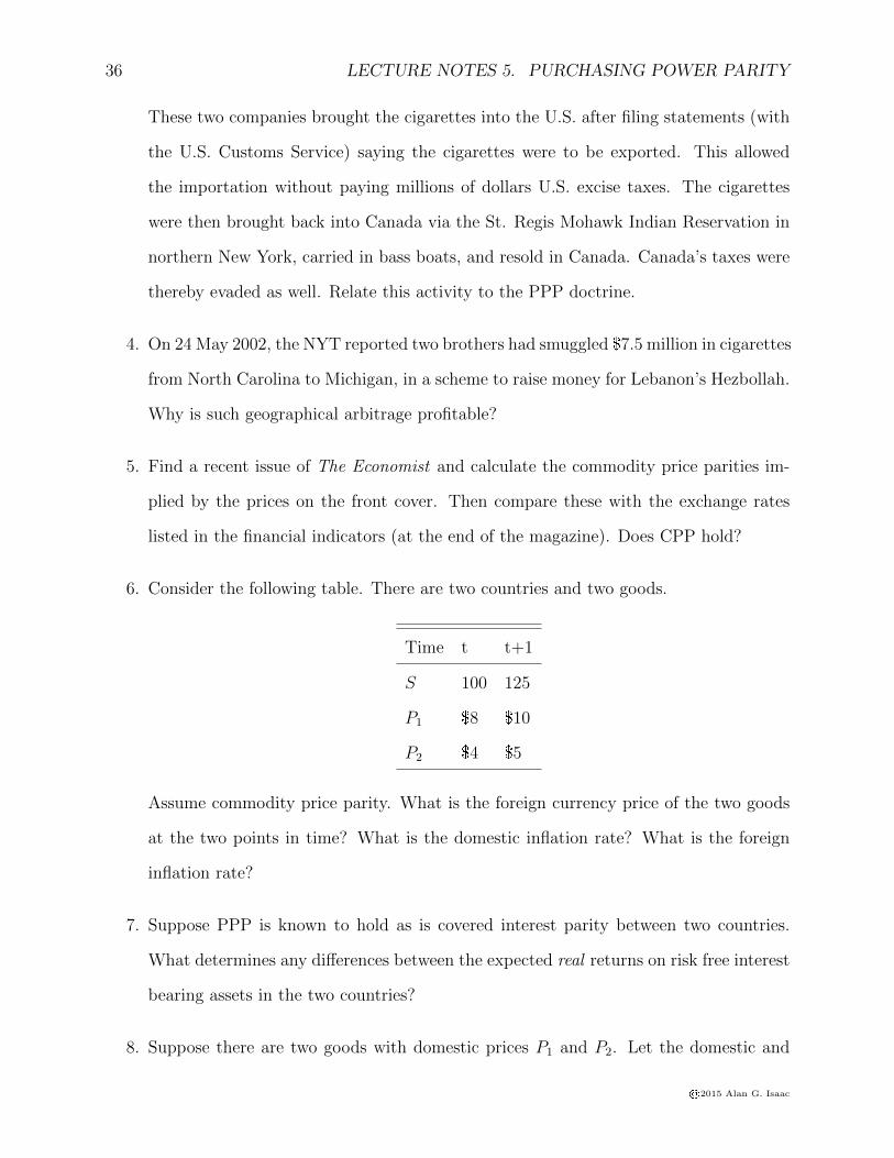
6. Consider the following table. There are two countries and two goods.

Time t t+1

S 100 125

P1 $8 $10

P2 $4 $5

Assume commodity price parity. What is the foreign currency price of the two goods

at the two points in time? What is the domestic inflation rate? What is the foreign

inflation rate?

7. Suppose PPP is known to hold as is covered interest parity between two countries.

What determines any differences between the expected real returns on risk free interest

bearing assets in the two countries?

8. Suppose there are two goods with domestic prices P1 and P2. Let the domestic and


37

foreign price indices be

P = P1βP2

1−β

P ∗ = P ∗1β∗P ∗21−β∗

Show that the real exchange rate is

Q =(SP ∗

1 )β∗(SP ∗

2 )1−β∗

P1βP2

1−β (5.27)

Clearly if the exchange rate and the commodity prices can move independently, then

the real exchange rate will fluctuate. Suppose however that CPP holds. Show that the

real exchange rate is then

Q =

(P1

P2

)β∗−β

(5.28)

Now as long as P1 and P2 change proportionately, so that the relative price P2/P1 is

unchanged, there is no change in the real exchange rate. but changes in the relative

price still cause changes in the real exchange rate. Finally, if set β = β∗ so that price

index construction is identical at home and abroad. Now what is the effect of changes

in relative prices on the PPP relationship?

9. Suppose that we use the same weights and the same goods to construct the domestic

and foreign price indices: CPI = f(P1, . . . , PN) and CPI ∗ = f(P ∗1 , . . . , P

∗N). Vanek

(1962, p.84) notes that our choice of f(·) will not affect our purchasing power parity

calculation if Pi/P∗i = k ∀i. Show this, using the first degree homogeneity of f(·).


Bibliography

Abauf, Niso and Philippe Jorion (1990, March). “Purchasing Power Parity in the Long

Run.” Journal of Finance 45(1), 157–174.

Adler, M. and B. Lehmann (1983, December). “Deviations from Purchasing Power Parity

in the Long-run.” Journal of Finance 38(5), 1471–87.

Argy, Victor (1994). International Macroeconomics. New York: Routledge.

Bilson, John F. O. (1981). “The Speculative Efficiency Hypothesis.” Journal of Business 54,

435–51.

Burstein, Ariel and Gita Gopinath (2014). “International Prices and Exchange Rates.” In

Elhanan Helpman, Kenneth Rogoff, and Gita Gopinath, eds., Handbook of International

Economics, Volume 4 of Handbooks in Economics, Chapter 7, pp. 391–452. Elsevier.

Cassel, Gustav (1918). “Abnormal Deviations in International Exchanges.” Economic Jour-

nal 28, 413–5.

Choi, Chi-Young, Nelson C. Mark, and Donggyu Sul (2006, June). “Unbiased Estimation

of the Half-Life to PPP Convergence in Panel Data.” Journal of Money, Credit and

Banking 38(4), pp. 921–938.

Cumby, Robert and Maurice Obstfeld (1984). “International Interest Rate and Price Level

Linkages under Flexible Exchange Rates: A Review of the Recent Evidence.” In

39

40 BIBLIOGRAPHY

J.F.O. Bilson and R.C. Marston, eds., Exchange Rate Theory and Practice, pp. 121–51.

Chicago: University of Chicago Press.

Einzig, Paul (1970). The History of Foreign Exchange. London: Macmillan.

Feenstra, Robert C. and Jon D. Kendall (1994, August). “Pass-Through of Exchange Rates

and Purchasing Power.” NBER Working Paper 4842, National Bureau of Economic

Research.

Frankel, Jeffrey (1990). “Zen and the Art of Modern Macroeconomics: The Search for Perfect

Nothingness.” In W. Haraf and T. Willett, eds., Monetary Policy for a Volativle Global

Economy. Washington, DC: American Enterprise Institute. Reprinted in (Frankel, 1993,

ch.7).

Frankel, Jeffrey and Kenneth Froot (1987, March). “Using Survey Data to Test Stan-

dard Propositions Regarding Exchange Rate Expectations.” American Economic Re-

view 77(1), 133–53.

Frankel, Jeffery A. (1986). “International Capital Mobility and Crowding Out in The U.S.

Economy: Imperfect Integration of Financial Markets or Goods Markets?” In R. Hafer,

ed., How Open Is The U.S. Economy?, pp. xxx. Lexington, MA: Lexington Books.

Frankel, Jeffrey A. (1993). On Exchange Rates. Cambridge, MA: The MIT Press.

Frankel, Jeffery A. and Andrew Rose (1996). “Mean Reversion Within and Between Coun-

tries: A Panel Project on Purchasing Power Parity.” Journal of International Eco-

nomics 40, 209–24.

Frenkel, Jacob A. (1978). “Purchasing Power Parity: Doctrinal Perspectives and Evidence

from the 1920s.” Journal of International Economics 8, 161–91.

Frenkel, Jacob A. (1981). “Flexible Exchange Rates, Prices and the Role of ‘News’: Lessons

from the 1970s.” Journal of Political Economy 89, 665–705.


BIBLIOGRAPHY 41

Froot, Kenneth A. and Kenneth Rogoff (1995). “Perspectives on PPP and the Long-Run

Real Exchange Rate.” In G.M. Grossman and K. Rogoff, eds., Handbook of International

Economics. Amsterdam: North-Holland.

Genberg, H. (1978). “Purchasing Power Parity under Fixed and Flexible Exchange Rates.”

Journal of International Economics 8, 247–76.

Hakkio, Craig S. (1985). “A Reexamination of Purchasing Power Parity: A Multi-Country

and Multi-Period Study.” Journal of International Economics 17, 265–77.

Helkie, William L. and Peter Hooper (1988). “An Empirical Analysis of the External Deficit

1980–86.” In Ralph C. Bryant, Gerald Holtham, and Peter Hooper, eds., External

Deficits and the Dollar: The Pit and the Pendulum, pp. 10–56. Washington, D.C.: The

Brookings Institution.

Heston, Alan and Robert Summers (1996, May). “International Price and Quantity Com-

parisons: Potentials and Pitfalls.” American Economic Review 86(2), 20–24.

Hodrick, Robert J. (1978). “An Empirical Analysis of the Monetary Approach to the Deter-

mination of the Exchange Rate.” In Jacob A. Frenkel and Harry G. Johnson, eds., The

Economics of Exchange Rates: Selected Studies, Chapter 6, pp. 97–116. Reading, MA:

Addison-Wesley.

Hooper, Peter and Jaime Marquez (1995). “Exchange Rates, Prices, and External Adjust-

ment.” In Peter B. Kenen, ed., Understanding Interdependence: The Macroeconomics

of the Open Economy. Princeton: Princeton University Press.

Houthakker, Hendrik S. (1962). Factors Affecting the United States Balance of Payments.

U.S. Government Printing Office.

Houthakker, Hendrik S. and Stephen P. Magee (1969, May). “Income and Price Elasticities

in World Trade.” Review of Economics and Statistics 51(2), 111–25.


42 BIBLIOGRAPHY

Huizinga, John H. (1987, Autumn). “An Empirical Investigation of the Long-run Behaviour

of Real Exchange Rates.” Carnegie-Rochester Conference Series on Public Policy 27,

149–214.

Isard, Peter (1977). “How Far Can We Push the Law of One Price?” American Economic

Review 67, 942–8.

Isard, Peter (1995). Exchange Rate Economics. Cambridge: Cambridge University Press.

Keynes, John Maynard (1925). The Economic Consequences of Mr. Churchill. London:

Hogarth Press.

Kravis, Irving B., Alan W. Heston, and Robert Summers (1978a, June). “Real GDP Per

Capita for more than One Hundred Countries.” Economic Journal 88(350), 215–42.

Kravis, Irving B., Alan W. Heston, and Robert Summers (1978b). United Nations Interna-

tional Comparison Project: Phase II; International Comparisons of Real Product and

Purchasing Power. Baltimore, MD: Johns Hopkins University Press.

Kravis, Irving B., Alan W. Heston, and Robert Summers (1982). World Product and Income.

Baltimore, MD: Johns Hopkins University Press.

Kravis, Irving B. and Robert E. Lipsey (1983). Toward an Explanation of National Price

Levels. Number 52 in Princeton Studies in International Finance. Princeton: Princeton

University Press.

Krugman, Paul (1978). “Purchasing Power Parity and Exchange Rates: Another Look at

the Evidence.” Journal of International Economics 8, 397–407.

Krugman, Paul (1989, May). “The J-Curve, the Fire Sale, and the Hard Landing.” American

Economic Review 79, 31–35.


BIBLIOGRAPHY 43

Krugman, Paul (1990). “Equilibrium Exchange Rates.” In William Branson, Jacob A.

Frenkel, and Morris Goldstein, eds., International Policy Coordinations and Exchange

Rate Fluctuations, pp. 159–87. Chicago: University of Chicago Press.

Lastrapes, William D. (1992, August). “Sources of Fluctuations in Real and Nominal Ex-

change Rates.” Review of Economics and Statistics 74(3), 530–9.

Lothian, James R. and Mark P. Taylor (1996, June). “Real Exchange Rate Behavior: The

Recent Float from the Perspective of the Past Two Centuries.” Journal of Political

Economy 104(3), 488–509.

MacDonald, Ronald (1993, November). “Long-Run Purchasing Power Parity: Is It For

Real?” Review of Economics and Statistics 75(4), 690–695.

Moggridge, Donald E. (1972). British Monetary Policy 1924–1931: The Norman Conquest

of $4.86. Cambridge: Cambridge University Press.

O’Connell, Paul G.J. and Shang-Jin Wei (2002, February). “ ‘The Bigger They Are the

Harder They Fall’: Retail Price Differences across U.S. Cities.” Journal of International

Economics 56(1), 21–53.

O’Connell, Paul G. J. (1998, February). “The Overvaluation of Purchasing Power Parity.”

Journal of International Economics 44(1), 1–19.

Officer, Lawrence H. (1976, March). “The Purchasing Power Parity Theory of Exchange

Rates: A Review Article.” International Monetary Fund Staff Papers 23, 1–60.

Officer, Lawrence H. (1980, May). “Effective Exchange Rates and Price Ratios over the

Long Run: A Test of the Purchasing-Power-Parity Theory.” Canadian Journal of Eco-

nomics 13(2), 206–230.

Oh, K.Y. (1996). “Purchasing Power Parity and Unit Root Tests Using Panel Data.” Journal

of International Money and Finance 15, 405–18.


44 BIBLIOGRAPHY

Pakko, Michael R. and Patricia S. Pollard (1996, January/February). “For Here or To

Go? Purchasing Power Parity and the Big Mac.” Federal Reserve Bank of St. Louis

Review 78(1), 3–21.

Papell, David H. (1997). “Searching for Stationarity: Purchasing Power Parity under the

Current Float.” Journal of International Economics 43(3–4), 313–332.

Patel, J. (1990, Oct.-Dec.). “Purchasing Power Parity as a Long-Run Relation.” Journal of

Applied Econometrics 5(4), 367–79.

Pigott, C. and R.J. Sweeney (1985). “Testing the Exchange Rate Implications of Two

Popular Monetary Models.” In S.W. Arnott, R.J. Sweeney, and T.D. Willet, eds.,

Exchange Rates, Trade and the US Economy. Ballinger.

Ricardo, David (1817). The Principles of Political Economy and Taxation. As reprinted

1987 by J.M. Dent & Sons, Ltd.

Rogoff, Kenneth (1996, June). “The Purchasing Power Parity Puzzle.” Journal of Economic

Literature 34, 647–668.

Roll, Richard (1979). “Violations of Purchasing Power Parity and Their Implications for Effi-

cient International Commodity Markets.” In Marshall Sarnat and Giorgio P. Szego, eds.,

International Finance and Trade, Volume 1, pp. 133–76. Cambridge, MA: Ballinger.

Samuelson, Paul A. (1964, May). “Theoretical Notes on Trade Problems.” Review of Eco-

nomics and Statistics 46(2), 145–54.

Summers, Robert and Alan Heston (1991, May). “The Penn World Table (Mark 5): An

Expanded Set of International Comparisons, 1950–1988.” Quarterly Journal of Eco-

nomics 106(2), 327–68.

Taylor, Mark P. (1988). “An Empirical Examination of Long-Run Purchasing Power Parity

Using Cointegration Techniques.” Applied Economics 20, 1369–81.


BIBLIOGRAPHY 45

Vanek, Jaroslav (1962). International Trade: Theory and Economic Policy. Homewood, IL:

Richard D. Irwin, Inc.

Williamson, John (1965). The Crawling Peg. Essays in International Finance. Princeton:

Princeton University Press.

Wu, Y. (1996). “Are Real Exchange Rates Nonstationary? Evidence from a Panel-Data

Test.” Journal of Money, Credit, and Banking 28, 54–63.

Young, J.P. (1925). “European Currency and Finance.” Technical Report Serial 9, Commis-

sion of Gold and Silver Enquiry.

Balassa-Samuelson

Define the foreign and domestic prices levels as weighted averages of traded and non-traded

goods prices:

p = (1− βpT + βpN (29)

p∗ = (1− β∗)p∗T + β∗p∗N (30)

Define the real exchange rate for tradeables:

qT = e+ p∗T − pT (31)

If absolute purchasing power parity held for all tradeables and the indices were identical,

we would have qT = 0.

Define the real exchange rate:

q = e+ p∗ − p

Work on the real exchange rate has found it to be non-stationary. There may still be

a LR relationship between the exchange rate and price levels, however, if we don’t impose


46 BIBLIOGRAPHY

homogeneity. Further, we may need to account for permanent shifts in the relative price of

tradeables.

q = e+ p∗ − p

= (qT − p∗T + pT ) + p∗ − p

= qT + β(pT − pN)− β∗(p∗T − p∗N)

Thus a rise in the domestic relative price of tradeable goods tends to depreciate the real

exchange rate.

Balassa (JPE,1964) notes that productivity grows faster in tradeable than non-tradable

goods sectors, and this is most true in faster growing countries. In light of our equation for

the real exchange rate, this suggests that faster growing countries will tend to experience real

appreciation. Other influences include the price of oil and the size and composition (i.e., is

the spending on traded or non-traded goods) of government expenditure. Zhou (SEJ, April

1995) uses these observations to write

rer = f(Poil, G,G∗, y − y∗,m−m∗)

Here y − y∗ is a productivity differential and m −m∗ is the monetary base differential.

Cointegration analysis (1973.1-1993.2 for Finland, Japan, US) found the monetary differen-

tial unimportant but the real shocks important determinants of the LR real exchange rates.

Oil price shocks were especially important; fiscal variables fairly important; productivity dif-

ferentials less so. Strauss (SEJ, April 1995) finds larger effects of the productivity differential

for 10 countries with annual data (1960-1990), but omits oil prices. He also tests directly for

relative price effects, which generally are also important. However the productivity effects do

not appear to be working throught the relative price channel, as the two are not cointegrated!

An error correction model indicates that the relative price of non-tradeables is an impor-

tant determinant of short run movements in the real exchange rate. Note: Strauss actually


BIBLIOGRAPHY 47

constructs relative productivity measures! (Most people just use industrial productivity.)

Appendix on Balassa-Samuelson

We will begin with commodity price parity for internationally traded goods, so that our

indices of traded goods prices, PT and P ∗T , bear the relationship

PT = KSP ∗T (32)

The constant K can deviate from unity to allow for real factors and price index construction.

Traded goods prices and non-traded goods prices, PNT and P ∗NT , contribute to the overall

price level.

P = f(PT , PNT ) (33)

P ∗ = f ∗(P ∗T , P

∗NT ) (34)

Take our standard representation of the real exchange rate

Q = SP ∗

P(35)

and substitute for the price indices to get the following.

Q = Sf ∗(P ∗

T , P∗NT )

f(PT , PNT )

= KPTP ∗T

f ∗(P ∗T , P

∗NT )

f(PT , PNT )

= Kf ∗(1, P ∗

NT/P∗T )

f(1, PNT/PT )

(36)

Thus changes in the relative price of non-traded goods affect the exchange rate.

To get a sense of the contribution of wages and productivities to real exchange rates,


48 BIBLIOGRAPHY

model price determination with a markup pricing model.

PT = µTWT

AT(37)

PNT = µNWNT

ANT(38)

P ∗T = µ∗

T

W ∗T

A∗T

(39)

P ∗NT = µ∗

N

W ∗NT

A∗NT

(40)

This gives us relative prices:

PNTPT

= µWNT/ANTWT/AT

=WNT/WT

ANT/ATP ∗NT

P ∗T

= µ∗W∗NT/A

∗NT

W ∗T/A

∗T

=W ∗NT/W

∗T

A∗NT/A

∗T

where µ = µNT/µT .

Therefore

QKf ∗(1,

W ∗NT /W

∗T

A∗NT /A

∗T

)

f(1, WNT /WT

ANT /AT)

(41)

For example, if

P = PT1−αPNT

α (42)

P ∗ = P ∗T1−α∗

P ∗NT

α∗(43)

so that our real exchange rate solution implies

Q = K

(P ∗NT

P ∗T

)α∗ (PTPNT

)α

(44)


BIBLIOGRAPHY 49

Then we end up with

Q = Kµ∗α∗

µα

(W ∗NT/W

∗T

A∗NT/A

∗T

)α∗ (WNT/WT

ANT/AT

)−α

(45)

Thus we see that deviations in relative wages or in relative productivities can cause deviations

from PPP.

Traditionally the Balassa-Samuelson model has been interpreted as linking the real ex-

change rate to relative productivities. Since the real exchange is subject to large short-run

fluctuations, it is clear that the Balassa-Samuelson link must be seen as a long-run expla-

nation of real exchange rate determination. See Asea and Corden (1994) and Froot and

Rogoff (1995) for recent surveys of the literature.

Canzoneri et al. (1996) find evidence in a panel of 13 OECD countries that the relative

price of nontraded goods reflects relative labor productivities, but they assume a common

wage across traded and nontraded sectors. Strauss and Ferris construct GDP price indices,

productivity measures, and real wage compensation rates for the traded and nontraded sec-

tors of 14 OECD countries for the years 1970–1990. They provide evidence that productivity

growth is higher in the traded goods sector, and that real (product) wage growth in each

sector tends to match that sector’s productivity growth. They find intersectoral wage growth

appears to influence the relative price of nontradables more than differences in productivity

growth.

Much empirical work has relied on total factor productivity measures of labor produci-

tivity. Canzoneri et al. (1996) argue for using the average product of labor as this gets rid

of the need for data on sectoral capital stocks or labor’s share in production. They also

note that for a broad range of technology, marginal and average products are proportional.

For example, if both capital and labor are mobile, CES production functions with constant

returns to scale imply this proportionality for perfectly competitive, profit-maximizing firms.


50 BIBLIOGRAPHY

If capital is not mobile, then let traded and nontraded goods be produced according to

T = F (KT )LTµT , N = G(KN)LN

µN (46)

This technology obviously includes the Cobb-Douglas technology as a special case. An

implication is the proportionality between average and marginal products.

∂T/∂LT = µTF (KT )LTµT−1 = µTT/LT = µTAT (47)

∂N/∂LN = µNF (KN)LNµN−1 = µNN/LN = µNAN (48)

For perfectly competitive profit maximizing firms, the marginal product of labor equals

the real product wage. Thus technology leading to equations (47) and (48) implies for

competitive firms the relationships (37)–(40).

Since tastes, technology, and factor endowments can all influence the relative price of

traded and nontraded goods, all offer themselves a potential explanantions. Kravis and

Lipsey (1983,1988) and Bhagwati (1984) emphasize the role of factor endowments, and Dorn-

busch, Fischer, and Samuelson (1977) emphasize the role of technology.


Bibliography

Abauf, Niso and Philippe Jorion (1990, March). “Purchasing Power Parity in the Long

Run.” Journal of Finance 45(1), 157–174.

Adler, M. and B. Lehmann (1983, December). “Deviations from Purchasing Power Parity

in the Long-run.” Journal of Finance 38(5), 1471–87.

Argy, Victor (1994). International Macroeconomics. New York: Routledge.

Bilson, John F. O. (1981). “The Speculative Efficiency Hypothesis.” Journal of Business 54,

435–51.

Burstein, Ariel and Gita Gopinath (2014). “International Prices and Exchange Rates.” In

Elhanan Helpman, Kenneth Rogoff, and Gita Gopinath, eds., Handbook of International

Economics, Volume 4 of Handbooks in Economics, Chapter 7, pp. 391–452. Elsevier.

Cassel, Gustav (1918). “Abnormal Deviations in International Exchanges.” Economic Jour-

nal 28, 413–5.

Choi, Chi-Young, Nelson C. Mark, and Donggyu Sul (2006, June). “Unbiased Estimation

of the Half-Life to PPP Convergence in Panel Data.” Journal of Money, Credit and

Banking 38(4), pp. 921–938.

Cumby, Robert and Maurice Obstfeld (1984). “International Interest Rate and Price Level

Linkages under Flexible Exchange Rates: A Review of the Recent Evidence.” In

51

52 BIBLIOGRAPHY

J.F.O. Bilson and R.C. Marston, eds., Exchange Rate Theory and Practice, pp. 121–51.

Chicago: University of Chicago Press.

Einzig, Paul (1970). The History of Foreign Exchange. London: Macmillan.

Feenstra, Robert C. and Jon D. Kendall (1994, August). “Pass-Through of Exchange Rates

and Purchasing Power.” NBER Working Paper 4842, National Bureau of Economic

Research.

Frankel, Jeffrey (1990). “Zen and the Art of Modern Macroeconomics: The Search for Perfect

Nothingness.” In W. Haraf and T. Willett, eds., Monetary Policy for a Volativle Global

Economy. Washington, DC: American Enterprise Institute. Reprinted in (Frankel, 1993,

ch.7).

Frankel, Jeffrey and Kenneth Froot (1987, March). “Using Survey Data to Test Stan-

dard Propositions Regarding Exchange Rate Expectations.” American Economic Re-

view 77(1), 133–53.

Frankel, Jeffery A. (1986). “International Capital Mobility and Crowding Out in The U.S.

Economy: Imperfect Integration of Financial Markets or Goods Markets?” In R. Hafer,

ed., How Open Is The U.S. Economy?, pp. xxx. Lexington, MA: Lexington Books.

Frankel, Jeffrey A. (1993). On Exchange Rates. Cambridge, MA: The MIT Press.

Frankel, Jeffery A. and Andrew Rose (1996). “Mean Reversion Within and Between Coun-

tries: A Panel Project on Purchasing Power Parity.” Journal of International Eco-

nomics 40, 209–24.

Frenkel, Jacob A. (1978). “Purchasing Power Parity: Doctrinal Perspectives and Evidence

from the 1920s.” Journal of International Economics 8, 161–91.

Frenkel, Jacob A. (1981). “Flexible Exchange Rates, Prices and the Role of ‘News’: Lessons

from the 1970s.” Journal of Political Economy 89, 665–705.


BIBLIOGRAPHY 53

Froot, Kenneth A. and Kenneth Rogoff (1995). “Perspectives on PPP and the Long-Run

Real Exchange Rate.” In G.M. Grossman and K. Rogoff, eds., Handbook of International

Economics. Amsterdam: North-Holland.

Genberg, H. (1978). “Purchasing Power Parity under Fixed and Flexible Exchange Rates.”

Journal of International Economics 8, 247–76.

Hakkio, Craig S. (1985). “A Reexamination of Purchasing Power Parity: A Multi-Country

and Multi-Period Study.” Journal of International Economics 17, 265–77.

Helkie, William L. and Peter Hooper (1988). “An Empirical Analysis of the External Deficit

1980–86.” In Ralph C. Bryant, Gerald Holtham, and Peter Hooper, eds., External

Deficits and the Dollar: The Pit and the Pendulum, pp. 10–56. Washington, D.C.: The

Brookings Institution.

Heston, Alan and Robert Summers (1996, May). “International Price and Quantity Com-

parisons: Potentials and Pitfalls.” American Economic Review 86(2), 20–24.

Hodrick, Robert J. (1978). “An Empirical Analysis of the Monetary Approach to the Deter-

mination of the Exchange Rate.” In Jacob A. Frenkel and Harry G. Johnson, eds., The

Economics of Exchange Rates: Selected Studies, Chapter 6, pp. 97–116. Reading, MA:

Addison-Wesley.

Hooper, Peter and Jaime Marquez (1995). “Exchange Rates, Prices, and External Adjust-

ment.” In Peter B. Kenen, ed., Understanding Interdependence: The Macroeconomics

of the Open Economy. Princeton: Princeton University Press.

Houthakker, Hendrik S. (1962). Factors Affecting the United States Balance of Payments.

U.S. Government Printing Office.

Houthakker, Hendrik S. and Stephen P. Magee (1969, May). “Income and Price Elasticities

in World Trade.” Review of Economics and Statistics 51(2), 111–25.


54 BIBLIOGRAPHY

Huizinga, John H. (1987, Autumn). “An Empirical Investigation of the Long-run Behaviour

of Real Exchange Rates.” Carnegie-Rochester Conference Series on Public Policy 27,

149–214.

Isard, Peter (1977). “How Far Can We Push the Law of One Price?” American Economic

Review 67, 942–8.

Isard, Peter (1995). Exchange Rate Economics. Cambridge: Cambridge University Press.

Keynes, John Maynard (1925). The Economic Consequences of Mr. Churchill. London:

Hogarth Press.

Kravis, Irving B., Alan W. Heston, and Robert Summers (1978a, June). “Real GDP Per

Capita for more than One Hundred Countries.” Economic Journal 88(350), 215–42.

Kravis, Irving B., Alan W. Heston, and Robert Summers (1978b). United Nations Interna-

tional Comparison Project: Phase II; International Comparisons of Real Product and

Purchasing Power. Baltimore, MD: Johns Hopkins University Press.

Kravis, Irving B., Alan W. Heston, and Robert Summers (1982). World Product and Income.

Baltimore, MD: Johns Hopkins University Press.

Kravis, Irving B. and Robert E. Lipsey (1983). Toward an Explanation of National Price

Levels. Number 52 in Princeton Studies in International Finance. Princeton: Princeton

University Press.

Krugman, Paul (1978). “Purchasing Power Parity and Exchange Rates: Another Look at

the Evidence.” Journal of International Economics 8, 397–407.

Krugman, Paul (1989, May). “The J-Curve, the Fire Sale, and the Hard Landing.” American

Economic Review 79, 31–35.


BIBLIOGRAPHY 55

Krugman, Paul (1990). “Equilibrium Exchange Rates.” In William Branson, Jacob A.

Frenkel, and Morris Goldstein, eds., International Policy Coordinations and Exchange

Rate Fluctuations, pp. 159–87. Chicago: University of Chicago Press.

Lastrapes, William D. (1992, August). “Sources of Fluctuations in Real and Nominal Ex-

change Rates.” Review of Economics and Statistics 74(3), 530–9.

Lothian, James R. and Mark P. Taylor (1996, June). “Real Exchange Rate Behavior: The

Recent Float from the Perspective of the Past Two Centuries.” Journal of Political

Economy 104(3), 488–509.

MacDonald, Ronald (1993, November). “Long-Run Purchasing Power Parity: Is It For

Real?” Review of Economics and Statistics 75(4), 690–695.

Moggridge, Donald E. (1972). British Monetary Policy 1924–1931: The Norman Conquest

of $4.86. Cambridge: Cambridge University Press.

O’Connell, Paul G.J. and Shang-Jin Wei (2002, February). “ ‘The Bigger They Are the

Harder They Fall’: Retail Price Differences across U.S. Cities.” Journal of International

Economics 56(1), 21–53.

O’Connell, Paul G. J. (1998, February). “The Overvaluation of Purchasing Power Parity.”

Journal of International Economics 44(1), 1–19.

Officer, Lawrence H. (1976, March). “The Purchasing Power Parity Theory of Exchange

Rates: A Review Article.” International Monetary Fund Staff Papers 23, 1–60.

Officer, Lawrence H. (1980, May). “Effective Exchange Rates and Price Ratios over the

Long Run: A Test of the Purchasing-Power-Parity Theory.” Canadian Journal of Eco-

nomics 13(2), 206–230.

Oh, K.Y. (1996). “Purchasing Power Parity and Unit Root Tests Using Panel Data.” Journal

of International Money and Finance 15, 405–18.


56 BIBLIOGRAPHY

Pakko, Michael R. and Patricia S. Pollard (1996, January/February). “For Here or To

Go? Purchasing Power Parity and the Big Mac.” Federal Reserve Bank of St. Louis

Review 78(1), 3–21.

Papell, David H. (1997). “Searching for Stationarity: Purchasing Power Parity under the

Current Float.” Journal of International Economics 43(3–4), 313–332.

Patel, J. (1990, Oct.-Dec.). “Purchasing Power Parity as a Long-Run Relation.” Journal of

Applied Econometrics 5(4), 367–79.

Pigott, C. and R.J. Sweeney (1985). “Testing the Exchange Rate Implications of Two

Popular Monetary Models.” In S.W. Arnott, R.J. Sweeney, and T.D. Willet, eds.,

Exchange Rates, Trade and the US Economy. Ballinger.

Ricardo, David (1817). The Principles of Political Economy and Taxation. As reprinted

1987 by J.M. Dent & Sons, Ltd.

Rogoff, Kenneth (1996, June). “The Purchasing Power Parity Puzzle.” Journal of Economic

Literature 34, 647–668.

Roll, Richard (1979). “Violations of Purchasing Power Parity and Their Implications for Effi-

cient International Commodity Markets.” In Marshall Sarnat and Giorgio P. Szego, eds.,

International Finance and Trade, Volume 1, pp. 133–76. Cambridge, MA: Ballinger.

Samuelson, Paul A. (1964, May). “Theoretical Notes on Trade Problems.” Review of Eco-

nomics and Statistics 46(2), 145–54.

Summers, Robert and Alan Heston (1991, May). “The Penn World Table (Mark 5): An

Expanded Set of International Comparisons, 1950–1988.” Quarterly Journal of Eco-

nomics 106(2), 327–68.

Taylor, Mark P. (1988). “An Empirical Examination of Long-Run Purchasing Power Parity

Using Cointegration Techniques.” Applied Economics 20, 1369–81.


BIBLIOGRAPHY 57

Vanek, Jaroslav (1962). International Trade: Theory and Economic Policy. Homewood, IL:

Richard D. Irwin, Inc.

Williamson, John (1965). The Crawling Peg. Essays in International Finance. Princeton:

Princeton University Press.

Wu, Y. (1996). “Are Real Exchange Rates Nonstationary? Evidence from a Panel-Data

Test.” Journal of Money, Credit, and Banking 28, 54–63.

Young, J.P. (1925). “European Currency and Finance.” Technical Report Serial 9, Commis-

sion of Gold and Silver Enquiry.


lecture notes 5 purchasing power parity - american … · lecture notes 5 purchasing power parity...

Documents