purchasing power parity. a survey on east european

AAccaaddeemmyy ooff EEccoonnoommiicc SSttuuddiieess,, BBuucchhaarreesstt

DDooccttoorraall SScchhooooll ooff FFiinnaannccee aanndd BBaannkkiinngg DDOOFFIINN

Dissertation Paper

Purchasing Power Parity. A Survey on East

European Countries (1995-2001)

MSc Student: Ioana Ceanga

Supervisor: Professor Moisa Altar

Bucharest, June 2002

Purchasing Power Parity (Summary)

1.Introduction

In this paper I tried to apply the theory of purchasing power parity (all the three

forms of it: absolute, semi-strong and relative) to explore the behavior of Romania’s,

Hungary’s, Poland’s and Czech Republic’s bilateral exchange rates with United States.

The study is based on a sample of monthly data for the period 1995:01 – 2001:12.

The PPP hypothesis has been widely discussed and analyzed since it was first put

forward by Cassel, and criticism of its validity has been intense on both theoretical and

empirical grounds. Yet its intuitive appeal and simplicity make the PPP hypothesis one of

the most popular economic theories of all the time. A strict interpretation of this concept

is that, in the long run, exchange rate trends are determined predominantly by relative

price developments at home and abroad.

The theory of purchasing power parity is based on the notion of arbitrage across

goods markets and the Law of One Price. This law states that on the assumptions of a

Perfect Capital Market (no transaction costs, no trade barriers and complete certainty)

homogenous goods will sell for the same price on the home and foreign market after

conversion into a common numeraire: *

ii SPP =

Here Pi is the price of a good i expressed in domestic currency, S is the nominal

exchange rate expressed in units of domestic currency per unit of foreign currency (or the

price of the foreign currency) and Pi* is the price of good i expressed in foreign currency.

If this law holds for one good, than it should hold for a basket of goods, too: *

ttt PSP =

Here Pt is the domestic price index at time t, Pt* is the foreign price index at time t

and (2) represents the equation for the absolute purchasing power parity. This postulates

that variation in prices between countries will be matched by exchange rates; that is,

nominal exchange rates will reflect differences in inflation rates among countries. An

alternative representation, where continuous compounding is assumed, is:


*ttt pps −=

where st, pt and pt* are the natural log of St, Pt and Pt

* respectively.

A weaker version of PPP, based on the relaxation of the homogeneity and

symmetry conditions can be expressed as: *ttt pps γβα −+=

where the coefficients α, β and γ are positive constants. A semi-strong form,

which imposes the restriction β=γ, shows a stable relationship between the nominal

exchange rate and prices.

After 1970 researchers have focused on the relative PPP: *%%% PPS ∆−∆=∆

Empirical support for long run PPP has been established by many researchers.

Niso Abuaf and Philippe Jorion (1990) analyzed 80 years of USD/GBP and USD/FRF

exchange rates and concluded that the nominal exchange rate had no tendency to return to

any particular level over the entire period. On the contrary, the real exchange rate proved

a clear tendency to return to its central value. Maurice Obstfeld (1995) studied the

exchange rate changes and inflation over a period of 20 years (1973-1993) using data for

22 OECD countries and concluded that the long-run variation in exchange rate changes

across countries is largely dependent on differences in rates of inflation.

Alan Taylor investigated PPP since the late nineteenth century for a panel of 20

countries over one hundred years. The evidence for long-run PPP was favorable using

univariate and multivariate tests of higher power. McCloskey and Zecher (1984) argued

that PPP worked very well under the Anglo-American gold standard before 1914.

Diebold, Husted and Rush (1991) explored a very long run of nineteenth century data for

six countries, and found support for PPP based on the low-frequency information lacking

in short-sample studies. Lothian and M. P. Taylor verified studied two centuries of dollar-

franc-sterling data and verified PPP. Lothian (1990) also found evidence that real

exchange rates were stationary for JPY, USD, GBP and FRF for the period 1875-1986.


Lee (1978) and Officer (1982) found strong evidence in favor of PPP based on analysis

of long time-series running from 1914 to the managed float of the 1970s, too.

Recent empirical research, mostly based on the time-series analysis of short spans

of data for the floating-rate era led many to conclude that PPP failed to hold, and that the

real exchange rate followed a random walk, with no mean-reversion property (the

tendency for a series to wander away from its stationary value and then return at later

points in time). However, new and higher-powered techniques have been used and

proved that in the long run PPP does indeed hold: it appears from these studies that real

exchange rates exhibit mean reversion with half-life of deviations of four to five years.

Razzaghipour, Fleming and Heaney found evidence of PPP analyzing quarterly-

series of five countries of East Asia during the period 1971:4-1997:2. Tang and Butiong

(1994) also examined the bilateral exchange rates of eleven developing Asian countries

during the period of 1973-1990 using an error correction model and found strong

evidence for PPP being a long run constraint for five of the countries. Hardouvelis and

Malliaropulos (2000) test long run PPP as a relationship between the exchange rate and

long-run equilibrium price differentials and apply this methodology to monthly data for

the Greek drachma, finding support for their version of PPP.

2. Data and methods

In order to see if the absolute PPP and the semi-strong PPP hold I used the

Johansen Test for Cointegration. In this way I studied the existence of unrestricted

stationary relationships linking bilateral nominal exchange rates and consumer price

indexes. Johansen’s cointegration model framework has the advantage of allowing for

joint determination of nominal exchange rates and CPIs, takes into account short term

dynamics of these variables while allowing for the return of the system to a long-term

equilibrium in line with PPP theory.

In order to apply this test all the variables I use have to be integrated of order one

(I(1)). The purpose of cointegration test is to determine if a group of non-stationary series


are cointegrated or not. The presence of a cointegrating relation forms the basis of the

VEC specification. The methodology developed by Johansen starts from considering a

VAR of order p:

tptpttt ByAyAyAy ε++++= −−− ...2211 (8)

where yt is a vector of non-stationary variables, B is a constant and εt is a vector of

random disturbances assumed to be identically and independently normally distributed.

All Ai terms represent coefficient matrices. We can rewrite the equation (8) as followed:

∑−

=−− ++∆Γ+Π=∆

1

11

p

itititt Byyy ε (9)

where ∑=

−=Πp

ii IA

1, and ∑

+=

−=Γp

ijji A

1.

The purpose of the cointegration model is to establish the number of long run

stationary relations among the variables contained in yt. In other words in this way we

may determine the number of cointegrated vectors by studying the rank of the matrix Π.

If the matrix mentioned above has rank zero, this means that there is no

cointegrating relationship between the variables. On the contrary, if the matrix Π has the

rank equal to n (the dimension of the vector yt) then yt is stationary. If the rank of Π is

bigger than one, but less than n, then the matrix can be decomposed into to full rank

matrices: α∈Mnxr and β∈Mrxn with Π=αβ`. The α matrix represents the matrix of

adjustment or error-correction coefficients. Its elements indicate the speed at which

endogenous variables return to equilibrium after a shock on the exogenous ones. The β

matrix is called the matrix of cointegrating vectors and r is the number of cointegrating

relations.

To determine the number of cointegrating relations conditional on the

assumptions made about the trend, we can proceed sequentially from r=0 to r=k-1 until

we fail to reject the null hypothesis. In order to test the null hypothesis we have to

calculate the followed statistic:


trace-statistic = ∑+=

−−n

riiLogT

1)1( λ ,

and to compare it with the 5% or 1% critical values from Osterwald-Lenum

(1992). Each λI represents the i-th largest eigenvalue of the matrix Π.

In order to verify the relative form of PPP I used an OLS estimation and I checked

through a Wald test if the coefficients estimated this way can be 1 or –1.

For the special case of a linear regression model

y = xβ+ε

and linear restrictions

0:0 =− rRH β

where R is a qxk matrix, and r is a q vector, respectively, the Wald statistic

reduces to:

( ) ( )( ) ( )rRbRXXRsrRbW −−=−− 112 ``` .

Bilateral exchange rates between the East European countries and United States

dollar, spanning the first month of 1995 to the twelfth month of 2001 were extracted from

the time series published by every central bank (Central Bank of Romania, Central Bank

of Poland, Central Bank of Hungary, Central Bank of Czech Republic and New York

Fed). The exchange rates are monthly average units of national currency per USD. The

consumer price indexes that I used for Romania, Czech Republic, Hungary, Poland and

United States cover the same period (1995:01-2001:12) and are set to 100 in 1994:12 for

all the countries. All initial data sets were normalized by dividing them with the

corresponding value in 1995:01. In order to linearize the relationships after normalizing

the series I converted them to natural logarithm.


3. Data and Econometric Results

3.1. Testing the strong form of PPP

Graph 1. Nominal exchange rates and consumer price indexes

0.0

0.5

1.0

1.5

2.0

2.5

3.0

3.5

1995 1996 1997 1998 1999 2000 2001

LNNFXRATE_RO LNNCPI_RO LNNCPI_US

0.0

0.2

0.4

0.6

0.8

1.0

1.2

1995 1996 1997 1998 1999 2000 2001

LNNFXRATE_HU LNNCPI_HU LNNCPI_US

-.1

.0

.1

.2

.3

.4

1995 1996 1997 1998 1999 2000 2001

LNNFXRATE_CZ LNNCPI_CZ LNNCPI_US

-.1

.0

.1

.2

.3

.4

.5

.6

.7

.8

1995 1996 1997 1998 1999 2000 2001

LNNFXRATE_PL LNNCPI_PL LNNCPI_US

I began analysis by testing the order of integration of the variables involved using

the ADF test. The results are shown in Table 1:

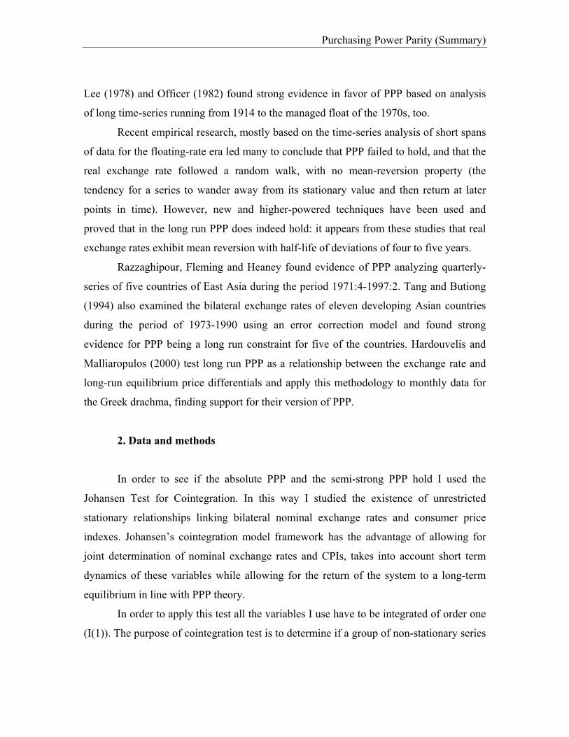
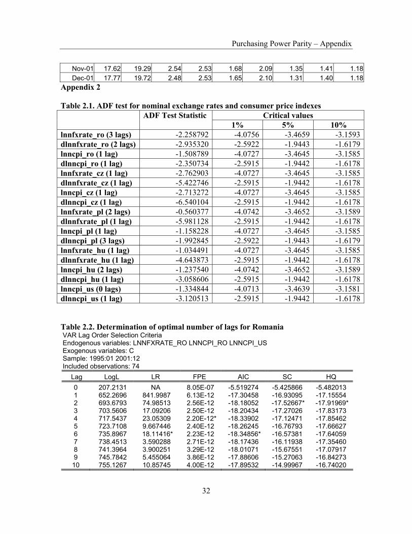
Table 1. ADF test for nominal exchange rates and consumer price indexes Critical values ADF Test Statistic

1% 5% 10% lnnfxrate_ro (3 lags) -2.258792 -4.0756 -3.4659 -3.1593dlnnfxrate_ro (2 lags) -2.935320 -2.5922 -1.9443 -1.6179lnncpi_ro (1 lag) -1.508789 -4.0727 -3.4645 -3.1585dlnncpi_ro (1 lag) -2.350734 -2.5915 -1.9442 -1.6178lnnfxrate_cz (1 lag) -2.762903 -4.0727 -3.4645 -3.1585dlnnfxrate_cz (1 lag) -5.422746 -2.5915 -1.9442 -1.6178


lnncpi_cz (1 lag) -2.713272 -4.0727 -3.4645 -3.1585dlnncpi_cz (1 lag) -6.540104 -2.5915 -1.9442 -1.6178lnnfxrate_pl (2 lags) -0.560377 -4.0742 -3.4652 -3.1589dlnnfxrate_pl (1 lag) -5.981128 -2.5915 -1.9442 -1.6178lnncpi_pl (1 lag) -1.158228 -4.0727 -3.4645 -3.1585dlnncpi_pl (3 lags) -1.992845 -2.5922 -1.9443 -1.6179lnnfxrate_hu (1 lag) -1.034491 -4.0727 -3.4645 -3.1585dlnnfxrate_hu (1 lag) -4.643873 -2.5915 -1.9442 -1.6178lnncpi_hu (2 lags) -1.237540 -4.0742 -3.4652 -3.1589dlnncpi_hu (1 lag) -3.058606 -2.5915 -1.9442 -1.6178lnncpi_us (0 lags) -1.334844 -4.0713 -3.4639 -3.1581dlnncpi_us (1 lag) -3.120513 -2.5915 -1.9442 -1.6178

Table 2. Johansen cointegration test for Romania Sample: 1995:01 2001:12 Included observations: 78 Test assumption: Linear deterministic trend in the data Series: LNNFXRATE_RO LNNCPI_RO LNNCPI_US Lags interval: 1 to 5

Likelihood 5 Percent 1 Percent Hypothesized Eigenvalue Ratio Critical Value Critical Value No. of CE(s) 0.238821 30.14110 29.68 35.65 None * 0.062167 8.855936 15.41 20.04 At most 1 0.048156 3.849620 3.76 6.65 At most 2 *

*(**) denotes rejection of the hypothesis at 5%(1%) significance level L.R. test indicates 1 cointegrating equation(s) at 5% significance level Unnormalized Cointegrating Coefficients: LNNFXRATE_

RO LNNCPI_RO LNNCPI_US

-2.517660 1.727848 12.96837 -0.443834 0.775963 -8.339995 0.040549 -0.256231 2.034686

Normalized Cointegrating Coefficients: 1 Cointegrating Equation(s)

LNNFXRATE_RO

LNNCPI_RO LNNCPI_US C

1.000000 -0.686291 -5.150962 -0.047947 (0.04205) (0.87199)

Log likelihood 773.5274


Table 3. Johansen cointegration test for Czech Republic Sample: 1995:01 2001:12 Included observations: 82 Test assumption: No deterministic trend in the data Series: LNNFXRATE_CZ LNNCPI_CZ LNNCPI_US Lags interval: 1 to 1

Likelihood 5 Percent 1 Percent Hypothesized Eigenvalue Ratio Critical Value Critical Value No. of CE(s) 0.312883 47.29511 34.91 41.07 None ** 0.122493 16.52460 19.96 24.60 At most 1 0.068398 5.809628 9.24 12.97 At most 2

*(**) denotes rejection of the hypothesis at 5%(1%) significance level L.R. test indicates 1 cointegrating equation(s) at 5% significance level

Unnormalized Cointegrating Coefficients: LNNFXRATE_

CZ LNNCPI_CZ LNNCPI_US C

0.453419 -0.252629 -0.963023 0.241994 1.951553 -2.070303 -0.380633 0.157147 -0.862068 -1.801182 6.174077 0.013245


LNNFXRATE_CZ

LNNCPI_CZ LNNCPI_US C

1.000000 -0.557164 -2.123911 0.533709 (0.93296) (2.49595) (0.36344)


Table 4. Johansen cointegration test for Poland Sample: 1995:01 2001:12 Included observations: 76 Test assumption: No deterministic trend in the data Series: LNNFXRATE_PL LNNCPI_PL LNNCPI_US Lags interval: 1 to 7




PL LNNCPI_PL LNNCPI_US C

1.835776 -3.712288 3.904466 1.183911


-3.220260 4.832239 -10.14059 -0.422439 -1.582787 -0.691088 10.96620 -0.116973

Normalized Cointegrating Coefficients: 1 Cointegrating Equation(s) LNNFXRATE_


1.000000 -2.022191 2.126875 0.644911 (0.28204) (0.97097) (0.13292)


Table 5. Johansen cointegration test for Hungary Sample: 1995:01 2001:12 Included observations: 74 Test assumption: No deterministic trend in the data Series: LNNFXRATE_HU LNNCPI_HU LNNCPI_US Lags interval: 1 to 9

Likelihood 5 Percent 1 Percent Hypothesized Eigenvalue Ratio Critical Value Critical Value No. of CE(s) 0.238779 27.76385 24.31 29.75 None * 0.092527 7.574298 12.53 16.31 At most 1 0.005250 0.389534 3.84 6.51 At most 2



HU LNNCPI_HU LNNCPI_US

4.855466 -5.454728 3.375489 6.017830 -3.346298 -20.59468 -1.792162 2.135273 1.653253



1.000000 -1.123420 0.695194 (0.14604) (1.06643)


3.2. Testing the semi-strong form of PPP

For testing the semi-strong form of PPP I applied the cointegration techniques on

an equation like:


ttt ds εγα ++=

where dt = pt – pt* represents bilateral relative prices (in logs), and the rest of the

notations remain the same as before except γ, the parameter on prices.

Table 6. ADF tests for bilateral relative prices

Critical values ADF Test Statistic 1% 5% 10%

ndif_ro (1 lag) -1.517107 -4.0727 -3.4645 -3.1585dndif_ro (0 lags) -2.937144 -2.5912 -1.9442 -1.6178rer_ro (2 lags) -1.484116 -2.5915 -1.9442 -1.6178ndif_cz (0 lags) -1.810165 -3.5101 -2.8963 -2.5851dndif_cz (0 lags) -9.188934 -2.5912 -1.9442 -1.6178rer_cz (0 lags) -1.734112 -2.5909 -1.9441 -1.6178ndif_pl (1 lag) -1.097155 -4.0727 -3.4645 -3.1585dndif_pl (1 lag) -3.134822 -2.5915 -1.9442 -1.6178rer_pl (1 lag) -3.354781 -4.0727 -3.4645 -3.1585ndif_hu (2 lags) -1.245060 -4.0742 -3.4652 -3.1589dndif_hu (2 lags) -2.630884 -2.5919 -1.9443 -1.6179rer_hu (1 lag) -2.148677 -4.0727 -3.4645 -3.1585 Table 7. Johansen cointegration test for Romania (semi-strong form) Sample: 1995:01 2001:12 Included observations: 80 Series: LNNFXRATE_RO NDIF_RO Lags interval: 1 to 3 Data Trend: None None Linear Linear Quadratic

Rank or No Intercept Intercept Intercept Intercept Intercept No. of CEs No Trend No Trend No Trend Trend Trend

Selected (5% level) Number of Cointegrating Relations by Model (columns) Trace 0 0 0 0 0

Table 8. Johansen cointegration test for Czech Republic (semi-strong form) Sample: 1995:01 2001:12 Included observations: 82 Series: LNNFXRATE_CZ NDIF_CZ Lags interval: 1 to 1 Data Trend: None None Linear Linear Quadratic




Table 9. Johansen cointegration test for Poland (semi-strong form) Sample: 1995:01 2001:12 Included observations: 77 Test assumption: No deterministic trend in the data Series: LNNFXRATE_PL NDIF_PL Lags interval: 1 to 6

Likelihood 5 Percent 1 Percent Hypothesized Eigenvalue Ratio Critical Value Critical Value No. of CE(s) 0.463406 52.99429 19.96 24.60 None ** 0.063612 5.060822 9.24 12.97 At most 1

*(**) denotes rejection of the hypothesis at 5%(1%) significance level L.R. test indicates 1 cointegrating equation(s) at 5% significance level Unnormalized Cointegrating Coefficients: LNNFXRATE_PL NDIF_PL C

1.273475 -1.286809 0.569549 2.609852 -1.692821 0.048741

Normalized Cointegrating Coefficients: 1 Cointegrating Equation(s) LNNFXRATE_PL NDIF_PL C

1.000000 -1.010470 0.447240 (0.09238) (0.12170)

Log likelihood 466.4346 Table 10. Johansen cointegration test for Hungary (semi-strong form) Sample: 1995:01 2001:12 Included observations: 76 Test assumption: No deterministic trend in the data Series: LNNFXRATE_HU NDIF_HU Lags interval: 1 to 7

Likelihood 5 Percent 1 Percent Hypothesized Eigenvalue Ratio Critical

Value Critical Value No. of CE(s)

0.541533 66.09440 19.96 24.60 None ** 0.085882 6.824503 9.24 12.97 At most 1

*(**) denotes rejection of the hypothesis at 5%(1%) significance level L.R. test indicates 1 cointegrating equation(s) at 5% significance level Unnormalized Cointegrating Coefficients: LNNFXRATE_HU NDIF_HU C

0.938251 -2.488686 1.153454 -3.394593 4.443984 -0.131305

Normalized Cointegrating Coefficients: 1 Cointegrating Equation(s) LNNFXRATE_HU NDIF_HU C

1.000000 -2.652475 1.229366 (0.51365) (0.45779)



3.3. Testing the relative form for PPP

The first step was to verify if the time-series are stationary or not. In this purpose

I used ADF test with the number of lags indicated by Akaike and Schwarz information

criterion. The results are shown in the Table 11:

Table 11. ADF test for the growth of nominal exchange rates and CPIs


dfxrate_ro (2 lags) -2.885920 -2.5919 -1.9443 -1.6179dcpi_ro (0 lags) -3.028379 -2.5912 -1.9442 -1.6178dfxrate_cz (0 lags) -6.383729 -2.5912 -1.9442 -1.6178dcpi_cz (0 lags) -9.046063 -2.5912 -1.9442 -1.6178dfxrate_pl (1 lag) -5.956909 -2.9515 -1.9442 -1.6178dcpi_pl (1 lag) -6.426192 -4.0742 -3.4652 -3.1589dfxrate_hu (0 lags) -5.537619 -2.5912 -1.9442 -1.6178dcpi_hu (1 lag) -5.828259 -4.0742 -3.4652 -3.1589dcpi_us (2 lags) -1.712843 -2.5919 -1.9443 -1.6179

Considering the fact that all the time-series proved to be stationary I can estimate

using the Ordinary Least Squares Method the coefficients of the equation from below:

tttt xxy εββα +++= 2211 (19)

where, yt is the growth of nominal exchange rates, x1t is the growth of the nationa

CPI, x2t is the growth of foreign CPI, α is the constant term, β1 and β2 are the coefficients

to be estimated and εt is the residual.


Table 12. OLS estimation for Romania Dependent Variable: DFXRATE_RO Method: Least Squares Sample(adjusted): 1995:03 2001:12 Included observations: 82 after adjusting endpoints Convergence achieved after 17 iterations

Variable Coefficient Std. Error t-Statistic Prob. DCPI_RO 1.441633 0.186418 7.733327 0.0000DCPI_US 0.935242 2.371850 0.394309 0.6944

DUMMY97 -0.385495 0.051071 -7.548178 0.0000C -0.014492 0.010531 -1.376118 0.1728

AR(1) 0.354268 0.120943 2.929219 0.0045R-squared 0.620423 Mean dependent var 0.036883Adjusted R-squared 0.600705 S.D. dependent var 0.056969S.E. of regression 0.035999 Akaike info criterion -3.751618Sum squared resid 0.099786 Schwarz criterion -3.604867Log likelihood 158.8163 F-statistic 31.46434Durbin-Watson stat 1.860417 Prob(F-statistic) 0.000000Inverted AR Roots .35 Table 13. OLS estimation for Czech Republic Dependent Variable: DFXRATE_CZ Method: Least Squares Sample(adjusted): 1995:03 2001:12 Included observations: 82 after adjusting endpoints Convergence achieved after 7 iterations

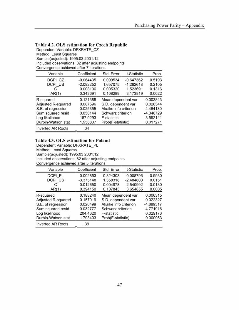
Variable Coefficient Std. Error t-Statistic Prob. DCPI_CZ -0.064435 0.099534 -0.647362 0.5193DCPI_US -2.092252 1.657075 -1.262618 0.2105

C 0.008106 0.005320 1.523691 0.1316AR(1) 0.343691 0.108289 3.173819 0.0022

R-squared 0.121388 Mean dependent var 0.003843Adjusted R-squared 0.087596 S.D. dependent var 0.026544S.E. of regression 0.025355 Akaike info criterion -4.464130Sum squared resid 0.050144 Schwarz criterion -4.346729Log likelihood 187.0293 F-statistic 3.592141Durbin-Watson stat 1.958837 Prob(F-statistic) 0.017271Inverted AR Roots .34


Table 14. OLS estimation for Poland Dependent Variable: DFXRATE_PL Method: Least Squares Sample(adjusted): 1995:03 2001:12 Included observations: 82 after adjusting endpoints Convergence achieved after 5 iterations

Variable Coefficient Std. Error t-Statistic Prob. DCPI_PL 0.002853 0.324303 0.008796 0.9930DCPI_US -3.375148 1.358318 -2.484800 0.0151

C 0.012650 0.004978 2.540992 0.0130AR(1) 0.394150 0.107843 3.654855 0.0005

R-squared 0.188240 Mean dependent var 0.006315Adjusted R-squared 0.157019 S.D. dependent var 0.022327S.E. of regression 0.020499 Akaike info criterion -4.889317Sum squared resid 0.032777 Schwarz criterion -4.771916Log likelihood 204.4620 F-statistic 6.029173Durbin-Watson stat 1.793403 Prob(F-statistic) 0.000953Inverted AR Roots .39 Table 15. OLS estimation for Hungary Dependent Variable: DFXRATE_HU Method: Least Squares Sample(adjusted): 1995:02 2001:12 Included observations: 83 after adjusting endpoints

Variable Coefficient Std. Error t-Statistic Prob. DCPI_HU 0.596563 0.231386 2.578219 0.0118DCPI_US -1.661401 1.267730 -1.310532 0.1938

C 0.007752 0.003801 2.039535 0.0447R-squared 0.082698 Mean dependent var 0.011209Adjusted R-squared 0.059765 S.D. dependent var 0.019396S.E. of regression 0.018807 Akaike info criterion -5.073658Sum squared resid 0.028297 Schwarz criterion -4.986230Log likelihood 213.5568 F-statistic 3.606121Durbin-Watson stat 1.644034 Prob(F-statistic) 0.031659

4. Conclusions

Tests performed in this paper for the East European developing countries

(Romania, Czech Republic, Poland and Hungary) indicate that the absolute, semi-strong

and relative forms of PPP relative to US dollar do not hold.

The reasons why PPP does not hold are plenty. One of them refers to the fact that

the assumption of no transaction costs is unrealistic. The large geographical distance


between United States and the East European countries I have studied is very important.

This implies sometimes very big transportation costs. In this case arbitrage will not take

place to take advantage of a deviation from parity unless the absolute magnitude of the

deviation is greater than the transport costs involved in undertaking the arbitrage. This

constraint has the effect of creating a “neutral band” within which no arbitrage

transactions will occur. So we’ll find the persistence of deviations from the PPP that are

smaller than transport cost.

The lack of commercial barriers imposed by the governments (like taxes) in order

to protect the domestic economy represents another assumption not found in real life.

These tariffs reduce the effective amount of funds available for arbitrage by an amount

(1-τ) where τ is the percentage tariff rate. Collecting a tax will widen the neutral band

within which no profitable arbitrage opportunities are available making more difficult the

PPP theory to hold.

According to Romania, another aspect that makes PPP not to hold is the

Romanian National Bank policy, which lately played a big part on the foreign exchange

market buying US dollars in order to increase the currency reserve which grew up to

almost 4 billion US dollars in the last few years. Also Romanian National Bank

intervened on the foreign exchange market almost every time there were pressures on the

national currency to appreciate.

Another problem with the PPP theory is represented by the costs of nontraded-

goods. Many items that are homogeneous, nevertheless sell for different prices because

they require a non-tradable input in the production process.

The law of one price assumes that individuals have good, even perfect,

information about the prices of goods in other markets. Only with this knowledge will

profit-seekers begin to export goods to the high price market and import goods from the

low priced market. Where there is imperfect information the law of one price may not

hold for some products which would imply that PPP would not hold either.

Notice that in the PPP equilibrium stories, it is the behavior of profit-seeking

importers and exporters that forces the exchange rate to adjust to the PPP level. But the


amount of daily currency transactions is more than ten times the amount of daily trade.

This fact would seem to suggest that the primary effect on the daily exchange rate must

be caused by the actions of investors rather than importers and exporters. Thus, the

participation of other traders in the foreign exchange market, who are motivated by other

concerns, may lead the exchange rate to a value that is not consistent with PPP.


References

1. Arghyrou, M. G. (2000), “Exchange Rate Pegging: Credibility and

Funadamentals. Evidence from Greece”, Brunel University

2. Engel, C. and J. C. Morley (2001), “The Adjustment of Prices and the Adjustment

of the Exchange Rate”, working paper 8550, www.nber.org

3. Greene, W.H. (1997), “Econometric Analysis”, Prentice Hall International, Inc.,

New Jersey, 789-796

4. Levich, R. M. (1998), “International Financial Markets. Prices and Policies”,

McGraw-Hill Co., London, 98-124

5. Maddala, G. S. (1998), “Introduction to Econometrics”, MacMillan Publishing

Company, New York, 577-601

6. Nagayasu, J. (1998), “Does the Long-Run PPP Hypothesis Hold for Africa?:

Evidence from Panel Co-Integration Study”, working paper 123, www.imf.org

7. Razzaghipour, A., G. A. Fleming, and R. A. Heaney (2000), “Purchasing Power

Parity and Emerging South East Asian Nations”, working paper #00-07, The

Australian National University

8. Schreyer, P. and F. Koechlin (2002), “Purchasing Power Parities – measurement

and uses”, working paper no.3, www.oecd.org

9. Steindel, C. (1997), “Are There Good Alternatives to the CPI?”, Current Issues in

Economics and Finance, 3(6), Federal Reserve Bank of New York

10. Taylor, A. M. (2000), “A Century of Purchasing Power Parity”, working paper

8012, www.nber.org

11. www.bnro.ro - National Bank of Romania

12. www.cnb.cz - National Bank of Czech Republic

13. www.imf.org - International Monetary Fund

14. www.mnb.hu - National Bank of Hungary

15. www.nbp.pl - National Bank of Poland

Purchasing Power Parity – Appendix

30

Appendix 1 Table 1.1. The normalized series converted to natural logarithm

ROMANIA HUNGARY POLAND CZECH REP. USA Month st pt st pt st pt st pt pt

Jan-95 1.00 1.00 1.00 1.00 1.00 1.00 1.00 1.00 1.00Feb-95 1.01 1.01 1.00 1.03 1.00 1.02 0.99 1.01 1.00Mar-95 1.03 1.02 1.04 1.07 0.98 1.04 0.94 1.01 1.00Apr-95 1.05 1.04 1.08 1.10 0.98 1.06 0.93 1.01 1.01

May-95 1.08 1.05 1.11 1.12 0.98 1.08 0.95 1.01 1.01Jun-95 1.10 1.06 1.13 1.14 0.96 1.09 0.94 1.01 1.01Jul-95 1.12 1.09 1.13 1.15 0.97 1.08 0.94 1.01 1.01

Aug-95 1.15 1.10 1.17 1.15 1.00 1.08 0.96 1.00 1.02Sep-95 1.18 1.12 1.20 1.17 1.01 1.12 0.97 1.00 1.02Oct-95 1.22 1.16 1.20 1.20 1.00 1.14 0.95 0.99 1.02Nov-95 1.35 1.21 1.22 1.22 1.02 1.15 0.95 0.99 1.02Dec-95 1.44 1.25 1.25 1.24 1.03 1.17 0.96 0.99 1.02Jan-96 1.46 1.27 1.27 1.29 1.03 1.21 0.97 1.09 1.03Feb-96 1.56 1.29 1.29 1.32 1.05 1.23 0.98 1.09 1.03Mar-96 1.62 1.31 1.31 1.34 1.06 1.25 0.98 1.10 1.03Apr-96 1.64 1.34 1.33 1.37 1.08 1.27 0.99 1.10 1.04

May-96 1.65 1.41 1.36 1.39 1.10 1.29 1.00 1.10 1.04Jun-96 1.68 1.42 1.37 1.41 1.12 1.30 1.00 1.09 1.04Jul-96 1.72 1.53 1.37 1.41 1.12 1.30 0.98 1.10 1.04


May-97 3.99 3.86 1.63 1.64 1.30 1.48 1.12 1.17 1.06Jun-97 4.04 3.95 1.66 1.67 1.33 1.50 1.17 1.17 1.06Jul-97 4.03 3.98 1.72 1.67 1.40 1.49 1.21 1.21 1.07

Aug-97 4.19 4.12 1.77 1.67 1.43 1.50 1.23 1.21 1.07Sep-97 4.24 4.25 1.76 1.70 1.42 1.52 1.21 1.20 1.07Oct-97 4.34 4.53 1.75 1.72 1.41 1.53 1.19 1.19 1.07Nov-97 4.40 4.73 1.76 1.74 1.44 1.55 1.19 1.19 1.07Dec-97 4.48 4.94 1.81 1.76 1.45 1.57 1.25 1.18 1.08Jan-98 4.67 5.18 1.85 1.81 1.45 1.62 1.27 1.32 1.08Feb-98 4.63 5.55 1.86 1.84 1.45 1.64 1.24 1.33 1.08Mar-98 4.62 5.76 1.89 1.86 1.42 1.65 1.22 1.33 1.08


31

Apr-98 4.72 5.92 1.90 1.88 1.40 1.67 1.22 1.32 1.08May-98 4.77 6.06 1.89 1.90 1.40 1.67 1.17 1.32 1.08Jun-98 4.83 6.14 1.94 1.91 1.43 1.68 1.20 1.31 1.08Jul-98 4.90 6.22 1.95 1.91 1.42 1.67 1.15 1.33 1.08


May-99 8.58 8.65 2.11 2.07 1.62 1.78 1.28 1.35 1.10Jun-99 8.87 9.09 2.15 2.08 1.62 1.78 1.29 1.34 1.10Jul-99 8.96 9.24 2.17 2.10 1.60 1.78 1.27 1.35 1.11


May-00 11.48 12.46 2.56 2.26 1.85 1.96 1.45 1.40 1.14Jun-00 11.84 12.81 2.45 2.27 1.81 1.97 1.37 1.39 1.14Jul-00 12.16 13.36 2.48 2.30 1.78 1.98 1.36 1.40 1.15


May-01 16.04 17.12 2.65 2.50 1.64 2.09 1.41 1.47 1.18Jun-01 16.30 17.39 2.59 2.51 1.63 2.09 1.43 1.47 1.18Jul-01 16.53 17.62 2.60 2.51 1.72 2.08 1.42 1.48 1.18

Aug-01 16.78 18.00 2.50 2.51 1.74 2.08 1.36 1.47 1.18Sep-01 17.02 18.35 2.52 2.52 1.73 2.08 1.35 1.44 1.18Oct-01 17.33 18.79 2.52 2.53 1.70 2.09 1.33 1.42 1.18


32

Nov-01 17.62 19.29 2.54 2.53 1.68 2.09 1.35 1.41 1.18Dec-01 17.77 19.72 2.48 2.53 1.65 2.10 1.31 1.40 1.18

Appendix 2 Table 2.1. ADF test for nominal exchange rates and consumer price indexes


lnnfxrate_ro (3 lags) -2.258792 -4.0756 -3.4659 -3.1593dlnnfxrate_ro (2 lags) -2.935320 -2.5922 -1.9443 -1.6179lnncpi_ro (1 lag) -1.508789 -4.0727 -3.4645 -3.1585dlnncpi_ro (1 lag) -2.350734 -2.5915 -1.9442 -1.6178lnnfxrate_cz (1 lag) -2.762903 -4.0727 -3.4645 -3.1585dlnnfxrate_cz (1 lag) -5.422746 -2.5915 -1.9442 -1.6178lnncpi_cz (1 lag) -2.713272 -4.0727 -3.4645 -3.1585dlnncpi_cz (1 lag) -6.540104 -2.5915 -1.9442 -1.6178lnnfxrate_pl (2 lags) -0.560377 -4.0742 -3.4652 -3.1589dlnnfxrate_pl (1 lag) -5.981128 -2.5915 -1.9442 -1.6178lnncpi_pl (1 lag) -1.158228 -4.0727 -3.4645 -3.1585dlnncpi_pl (3 lags) -1.992845 -2.5922 -1.9443 -1.6179lnnfxrate_hu (1 lag) -1.034491 -4.0727 -3.4645 -3.1585dlnnfxrate_hu (1 lag) -4.643873 -2.5915 -1.9442 -1.6178lnncpi_hu (2 lags) -1.237540 -4.0742 -3.4652 -3.1589dlnncpi_hu (1 lag) -3.058606 -2.5915 -1.9442 -1.6178lnncpi_us (0 lags) -1.334844 -4.0713 -3.4639 -3.1581dlnncpi_us (1 lag) -3.120513 -2.5915 -1.9442 -1.6178 Table 2.2. Determination of optimal number of lags for Romania VAR Lag Order Selection Criteria Endogenous variables: LNNFXRATE_RO LNNCPI_RO LNNCPI_US Exogenous variables: C Sample: 1995:01 2001:12 Included observations: 74

Lag LogL LR FPE AIC SC HQ 0 207.2131 NA 8.05E-07 -5.519274 -5.425866 -5.482013 1 652.2696 841.9987 6.13E-12 -17.30458 -16.93095 -17.15554 2 693.6793 74.98513 2.56E-12 -18.18052 -17.52667* -17.91969* 3 703.5606 17.09206 2.50E-12 -18.20434 -17.27026 -17.83173 4 717.5437 23.05309 2.20E-12* -18.33902 -17.12471 -17.85462 5 723.7108 9.667446 2.40E-12 -18.26245 -16.76793 -17.66627 6 735.8967 18.11416* 2.23E-12 -18.34856* -16.57381 -17.64059 7 738.4513 3.590288 2.71E-12 -18.17436 -16.11938 -17.35460 8 741.3964 3.900251 3.29E-12 -18.01071 -15.67551 -17.07917 9 745.7842 5.455064 3.86E-12 -17.88606 -15.27063 -16.84273 10 755.1267 10.85745 4.00E-12 -17.89532 -14.99967 -16.74020


33


34

Table 2.3. Determination of optimal number of lags for Czech Republic VAR Lag Order Selection Criteria Endogenous variables: LNNFXRATE_CZ LNNCPI_CZ LNNCPI_US Exogenous variables: C Sample: 1995:01 2001:12 Included observations: 74

Lag LogL LR FPE AIC SC HQ 0 362.1073 NA 1.22E-08 -9.705603 -9.612195 -9.668342 1 700.1664 639.5712 1.68E-12* -18.59909* -18.22546* -18.45004* 2 708.0169 14.21587 1.74E-12 -18.56803 -17.91417 -18.30719 3 711.9632 6.825984 2.00E-12 -18.43144 -17.49736 -18.05882 4 722.3378 17.10413* 1.93E-12 -18.46859 -17.25429 -17.98419 5 726.6092 6.695657 2.22E-12 -18.34079 -16.84626 -17.74460 6 733.2344 9.848290 2.40E-12 -18.27661 -16.50185 -17.56864 7 743.5258 14.46362 2.37E-12 -18.31151 -16.25653 -17.49175 8 748.0765 6.026507 2.74E-12 -18.19126 -15.85605 -17.25972 9 760.4613 15.39732 2.59E-12 -18.28274 -15.66731 -17.23941 10 771.6843 13.04295 2.56E-12 -18.34282 -15.44717 -17.18771

Table 2.4. Determination of optimal number of lags for Poland VAR Lag Order Selection Criteria Endogenous variables: LNNFXRATE_PL LNNCPI_PL LNNCPI_US Exogenous variables: C Sample: 1995:01 2001:12 Included observations: 74

Lag LogL LR FPE AIC SC HQ 0 385.7133 NA 6.46E-09 -10.34360 -10.25019 -10.30634 1 824.6280 830.3792 5.81E-14 -21.96292 -21.58929* -21.81387* 2 836.0639 20.70823 5.45E-14 -22.02875 -21.37490 -21.76792 3 842.7180 11.50976 5.83E-14 -21.96535 -21.03127 -21.59274 4 853.3806 17.57889 5.60E-14 -22.01029 -20.79598 -21.52589 5 858.2660 7.658191 6.32E-14 -21.89908 -20.40455 -21.30290 6 870.6354 18.38698 5.86E-14 -21.99015 -20.21539 -21.28218 7 888.4903 25.09325* 4.70E-14* -22.22947* -20.17449 -21.40971 8 897.3781 11.77033 4.85E-14 -22.22643 -19.89123 -21.29489 9 902.7896 6.727813 5.54E-14 -22.12945 -19.51402 -21.08612 10 908.7940 6.978106 6.29E-14 -22.04849 -19.15284 -20.89338


35

Table 2.5. Determination of optimal number of lags for Hungary VAR Lag Order Selection Criteria Endogenous variables: LNNFXRATE_HU LNNCPI_HU LNNCPI_US Exogenous variables: C Sample: 1995:01 2001:12 Included observations: 74

Lag LogL LR FPE AIC SC HQ 0 386.5429 NA 6.32E-09 -10.36603 -10.27262 -10.32876 1 827.8571 834.9187 5.33E-14 -22.05019 -21.67656* -21.90115* 2 837.4344 17.34261 5.25E-14 -22.06579 -21.41194 -21.80496 3 845.6270 14.17109 5.38E-14 -22.04397 -21.10989 -21.67136 4 855.1950 15.77425 5.33E-14 -22.05932 -20.84502 -21.57492 5 858.8144 5.673569 6.23E-14 -21.91390 -20.41937 -21.31772 6 880.4408 32.14738 4.49E-14 -22.25516 -20.48040 -21.54719 7 895.0386 20.51583 3.94E-14 -22.40645 -20.35147 -21.58669 8 913.2934 24.17536 3.15E-14 -22.65658 -20.32138 -21.72504 9 931.1953 22.25630* 2.57E-14* -22.89717* -20.28174 -21.85384 10 934.3989 3.723106 3.15E-14 -22.74051 -19.84486 -21.58540

* indicates lag order selected by the criterion LR: sequential modified LR test statistic (each test at 5% level) FPE: Final prediction error AIC: Akaike information criterion SC: Schwarz information criterion HQ: Hannan-Quinn information criterion Table 2.6. Johansen cointegration test for Romania Sample: 1995:01 2001:12 Included observations: 78 Test assumption: Linear deterministic trend in the data Series: LNNFXRATE_RO LNNCPI_RO LNNCPI_US Lags interval: 1 to 5

Likelihood 5 Percent 1 Percent Hypothesized Eigenvalue Ratio Critical Value Critical Value No. of CE(s) 0.238821 30.14110 29.68 35.65 None * 0.062167 8.855936 15.41 20.04 At most 1 0.048156 3.849620 3.76 6.65 At most 2 *

*(**) denotes rejection of the hypothesis at 5%(1%) significance level L.R. test indicates 1 cointegrating equation(s) at 5% significance level Unnormalized Cointegrating Coefficients: LNNFXRATE_

RO LNNCPI_RO LNNCPI_US

-2.517660 1.727848 12.96837 -0.443834 0.775963 -8.339995 0.040549 -0.256231 2.034686


LNNFXRATE_RO

LNNCPI_RO LNNCPI_US C


36

1.000000 -0.686291 -5.150962 -0.047947 (0.04205) (0.87199)


Table 2.7. Estimated VEC for (lnnfxrate_ro, lnncpi_ro, lnncpi_us) D(LNNFXRATE_RO) = - 0.2907547863*( LNNFXRATE_RO(-1) - 0.6862912733*LNNCPI_RO(-1) - 5.150961917*LNNCPI_US(-1) - 0.04794697665 ) + 0.9798504677*D(LNNFXRATE_RO(-1)) - 0.715630526*D(LNNFXRATE_RO(-2)) + 0.3987505767*D(LNNFXRATE_RO(-3)) - 0.02010604964*D(LNNFXRATE_RO(-4)) + 0.3951618513*D(LNNFXRATE_RO(-5)) + 0.620328767*D(LNNCPI_RO(-1)) + 0.1276815544*D(LNNCPI_RO(-2)) - 0.355187963*D(LNNCPI_RO(-3)) - 0.4572106337*D(LNNCPI_RO(-4)) + 0.2971998072*D(LNNCPI_RO(-5)) + 4.837993163*D(LNNCPI_US(-1)) + 3.177777702*D(LNNCPI_US(-2)) + 1.69965485*D(LNNCPI_US(-3)) + 0.504789438*D(LNNCPI_US(-4)) - 2.792475451*D(LNNCPI_US(-5)) - 0.02509245054 D(LNNCPI_RO) = 0.0453207507*( LNNFXRATE_RO(-1) - 0.6862912733*LNNCPI_RO(-1) - 5.150961917*LNNCPI_US(-1) - 0.04794697665 ) + 0.4140074194*D(LNNFXRATE_RO(-1)) - 0.03618840998*D(LNNFXRATE_RO(-2)) - 0.255531141*D(LNNFXRATE_RO(-3)) - 0.06038974788*D(LNNFXRATE_RO(-4)) - 0.04567100852*D(LNNFXRATE_RO(-5)) + 0.2530252818*D(LNNCPI_RO(-1)) + 0.4248832999*D(LNNCPI_RO(-2)) + 0.1269288892*D(LNNCPI_RO(-3)) - 0.1488072012*D(LNNCPI_RO(-4)) + 0.08421678589*D(LNNCPI_RO(-5)) + 1.636301145*D(LNNCPI_US(-1)) + 2.728500187*D(LNNCPI_US(-2)) - 0.5998073633*D(LNNCPI_US(-3)) + 1.022056226*D(LNNCPI_US(-4)) - 2.142415246*D(LNNCPI_US(-5)) + 0.004280139555 D(LNNCPI_US) = 0.006291130401*( LNNFXRATE_RO(-1) - 0.6862912733*LNNCPI_RO(-1) - 5.150961917*LNNCPI_US(-1) - 0.04794697665 ) + 0.001195734952*D(LNNFXRATE_RO(-1)) - 0.001603451068*D(LNNFXRATE_RO(-2)) + 0.002425195995*D(LNNFXRATE_RO(-3)) + 0.003093132199*D(LNNFXRATE_RO(-4)) - 0.01010358754*D(LNNFXRATE_RO(-5)) - 0.008847765966*D(LNNCPI_RO(-1)) - 0.01591815256*D(LNNCPI_RO(-2)) + 7.110363272e-05*D(LNNCPI_RO(-3)) + 0.007061071856*D(LNNCPI_RO(-4)) + 0.008055961783*D(LNNCPI_RO(-5)) + 0.05074119816*D(LNNCPI_US(-1)) - 0.2424440435*D(LNNCPI_US(-2)) + 0.4081486169*D(LNNCPI_US(-3)) + 0.2375381225*D(LNNCPI_US(-4)) + 0.197605476*D(LNNCPI_US(-5)) + 0.001104046951


37

Table 2.8. Johansen cointegration test for Czech Republic Sample: 1995:01 2001:12 Included observations: 82 Test assumption: No deterministic trend in the data Series: LNNFXRATE_CZ LNNCPI_CZ LNNCPI_US Lags interval: 1 to 1




CZ LNNCPI_CZ LNNCPI_US C

0.453419 -0.252629 -0.963023 0.241994 1.951553 -2.070303 -0.380633 0.157147 -0.862068 -1.801182 6.174077 0.013245


LNNFXRATE_CZ

LNNCPI_CZ LNNCPI_US C

1.000000 -0.557164 -2.123911 0.533709 (0.93296) (2.49595) (0.36344)


Table 2.9. Estimated VEC for (lnnfxrate_cz, lnncpi_cz, lnncpi_us) D(LNNFXRATE_CZ) = - 0.007399003598*( LNNFXRATE_CZ(-1) - 0.5571642272*LNNCPI_CZ(-1) - 2.123910877*LNNCPI_US(-1) + 0.5337092732 ) + 0.3326271786*D(LNNFXRATE_CZ(-1)) + 0.1511737549*D(LNNCPI_CZ(-1)) + 1.75752095*D(LNNCPI_US(-1)) D(LNNCPI_CZ) = 0.009814160202*( LNNFXRATE_CZ(-1) - 0.5571642272*LNNCPI_CZ(-1) - 2.123910877*LNNCPI_US(-1) + 0.5337092732 ) + 0.1444492271*D(LNNFXRATE_CZ(-1)) - 0.03367971593*D(LNNCPI_CZ(-1)) + 0.1887649466*D(LNNCPI_US(-1)) D(LNNCPI_US) = 0.004549679719*( LNNFXRATE_CZ(-1) - 0.5571642272*LNNCPI_CZ(-1) - 2.123910877*LNNCPI_US(-1) + 0.5337092732 ) - 0.0009751669295*D(LNNFXRATE_CZ(-1)) - 0.002662968159*D(LNNCPI_CZ(-1)) + 0.1143994998*D(LNNCPI_US(-1))


38

Table 2.10. Johansen cointegration test for Poland Sample: 1995:01 2001:12 Included observations: 76 Test assumption: No deterministic trend in the data Series: LNNFXRATE_PL LNNCPI_PL LNNCPI_US Lags interval: 1 to 7





1.835776 -3.712288 3.904466 1.183911 -3.220260 4.832239 -10.14059 -0.422439 -1.582787 -0.691088 10.96620 -0.116973



1.000000 -2.022191 2.126875 0.644911 (0.28204) (0.97097) (0.13292)


Table 2.11. Estimated VEC for (lnnfxrate_pl, lnncpi_pl, lnncpi_us) D(LNNFXRATE_PL) = - 0.04036419297*( LNNFXRATE_PL(-1) - 2.022190661*LNNCPI_PL(-1) + 2.126875215*LNNCPI_US(-1) + 0.6449106971 ) + 0.495007583*D(LNNFXRATE_PL(-1)) - 0.1293892853*D(LNNFXRATE_PL(-2)) - 0.05388162017*D(LNNFXRATE_PL(-3)) - 0.1291402978*D(LNNFXRATE_PL(-4)) + 0.1925203409*D(LNNFXRATE_PL(-5)) + 0.003062334063*D(LNNFXRATE_PL(-6)) - 0.05091211014*D(LNNFXRATE_PL(-7)) + 0.5219669784*D(LNNCPI_PL(-1)) + 0.02781567556*D(LNNCPI_PL(-2)) + 0.342160105*D(LNNCPI_PL(-3)) - 0.1251768166*D(LNNCPI_PL(-4)) + 0.4017093727*D(LNNCPI_PL(-5)) - 0.2752631613*D(LNNCPI_PL(-6)) + 0.5934835077*D(LNNCPI_PL(-7)) + 0.4035078414*D(LNNCPI_US(-1)) + 4.151977287*D(LNNCPI_US(-2)) - 2.421588625*D(LNNCPI_US(-3)) - 0.6629754854*D(LNNCPI_US(-4)) - 1.775168471*D(LNNCPI_US(-5)) - 1.508379283*D(LNNCPI_US(-6)) + 1.381147672*D(LNNCPI_US(-7)) D(LNNCPI_PL) = 0.06101562661*( LNNFXRATE_PL(-1) - 2.022190661*LNNCPI_PL(-1) + 2.126875215*LNNCPI_US(-1) + 0.6449106971 ) - 0.04097330186*D(LNNFXRATE_PL(-1)) - 0.01877065317*D(LNNFXRATE_PL(-2)) - 0.0699449129*D(LNNFXRATE_PL(-3)) - 0.03234688639*D(LNNFXRATE_PL(-4)) + 0.01853754948*D(LNNFXRATE_PL(-5)) - 0.05950447588*D(LNNFXRATE_PL(-6)) + 0.08772681484*D(LNNFXRATE_PL(-7)) + 0.04878045752*D(LNNCPI_PL(-1)) + 0.004491097166*D(LNNCPI_PL(-2)) -


39

0.007071998541*D(LNNCPI_PL(-3)) + 0.1433611674*D(LNNCPI_PL(-4)) - 0.07918343867*D(LNNCPI_PL(-5)) - 0.4685424334*D(LNNCPI_PL(-6)) - 0.06746076067*D(LNNCPI_PL(-7)) - 0.4060618702*D(LNNCPI_US(-1)) + 0.02376812128*D(LNNCPI_US(-2)) - 0.3341304254*D(LNNCPI_US(-3)) + 0.4300089305*D(LNNCPI_US(-4)) + 0.4869418941*D(LNNCPI_US(-5)) + 0.3833479766*D(LNNCPI_US(-6)) + 0.1966932551*D(LNNCPI_US(-7)) D(LNNCPI_US) = 0.002890273018*( LNNFXRATE_PL(-1) - 2.022190661*LNNCPI_PL(-1) + 2.126875215*LNNCPI_US(-1) + 0.6449106971 ) - 0.007951504009*D(LNNFXRATE_PL(-1)) + 0.006039526464*D(LNNFXRATE_PL(-2)) - 0.02155028776*D(LNNFXRATE_PL(-3)) + 0.03696512096*D(LNNFXRATE_PL(-4)) - 0.02946244229*D(LNNFXRATE_PL(-5)) + 0.01101148208*D(LNNFXRATE_PL(-6)) + 0.01125461806*D(LNNFXRATE_PL(-7)) + 0.001190419042*D(LNNCPI_PL(-1)) - 0.02425494755*D(LNNCPI_PL(-2)) - 0.017007277*D(LNNCPI_PL(-3)) + 0.04197460459*D(LNNCPI_PL(-4)) - 0.03653833092*D(LNNCPI_PL(-5)) + 0.04082945007*D(LNNCPI_PL(-6)) - 0.02744420963*D(LNNCPI_PL(-7)) + 0.2528199214*D(LNNCPI_US(-1)) - 0.2026574149*D(LNNCPI_US(-2)) + 0.4374412951*D(LNNCPI_US(-3)) + 0.1895015986*D(LNNCPI_US(-4)) + 0.09304870157*D(LNNCPI_US(-5)) - 0.1511530897*D(LNNCPI_US(-6)) + 0.1193541581*D(LNNCPI_US(-7)) Table 2.12. Johansen cointegration test for Hungary Sample: 1995:01 2001:12 Included observations: 74 Test assumption: No deterministic trend in the data Series: LNNFXRATE_HU LNNCPI_HU LNNCPI_US Lags interval: 1 to 9

Likelihood 5 Percent 1 Percent Hypothesized Eigenvalue Ratio Critical Value Critical Value No. of CE(s) 0.238779 27.76385 24.31 29.75 None * 0.092527 7.574298 12.53 16.31 At most 1 0.005250 0.389534 3.84 6.51 At most 2




4.855466 -5.454728 3.375489 6.017830 -3.346298 -20.59468 -1.792162 2.135273 1.653253



1.000000 -1.123420 0.695194 (0.14604) (1.06643)



40

Table 2.13. Estimated VEC for (lnnfxrate_hu, lnncpi_hu, lnncpi_us) D(LNNFXRATE_HU) = - 0.2366759823*( LNNFXRATE_HU(-1) - 1.123420155*LNNCPI_HU(-1) + 0.6951936788*LNNCPI_US(-1) ) + 0.2981580494*D(LNNFXRATE_HU(-1)) + 0.1408791248*D(LNNFXRATE_HU(-2)) - 0.1374268646*D(LNNFXRATE_HU(-3)) + 0.08100524522*D(LNNFXRATE_HU(-4)) + 0.4860635318*D(LNNFXRATE_HU(-5)) - 0.02108759325*D(LNNFXRATE_HU(-6)) + 0.1799154051*D(LNNFXRATE_HU(-7)) + 0.381969713*D(LNNFXRATE_HU(-8)) - 0.1219436291*D(LNNFXRATE_HU(-9)) + 0.4030081132*D(LNNCPI_HU(-1)) - 0.07220258538*D(LNNCPI_HU(-2)) - 0.5813762782*D(LNNCPI_HU(-3)) - 0.1028315605*D(LNNCPI_HU(-4)) - 0.2031325398*D(LNNCPI_HU(-5)) - 0.2560033732*D(LNNCPI_HU(-6)) + 0.1208383356*D(LNNCPI_HU(-7)) - 0.5921538353*D(LNNCPI_HU(-8)) - 0.4023481722*D(LNNCPI_HU(-9)) + 0.3393745404*D(LNNCPI_US(-1)) + 3.769481138*D(LNNCPI_US(-2)) + 0.09892637957*D(LNNCPI_US(-3)) - 2.830693918*D(LNNCPI_US(-4)) + 2.565406288*D(LNNCPI_US(-5)) - 1.196117071*D(LNNCPI_US(-6)) + 0.3523440259*D(LNNCPI_US(-7)) + 5.401000873*D(LNNCPI_US(-8)) - 0.2461781037*D(LNNCPI_US(-9)) D(LNNCPI_HU) = - 0.05000773191*( LNNFXRATE_HU(-1) - 1.123420155*LNNCPI_HU(-1) + 0.6951936788*LNNCPI_US(-1) ) - 0.008498087477*D(LNNFXRATE_HU(-1)) + 0.01136336839*D(LNNFXRATE_HU(-2)) - 0.03038546435*D(LNNFXRATE_HU(-3)) + 0.07175210078*D(LNNFXRATE_HU(-4)) + 0.1193051114*D(LNNFXRATE_HU(-5)) + 0.0965030465*D(LNNFXRATE_HU(-6)) - 0.02056965328*D(LNNFXRATE_HU(-7)) + 0.0633961115*D(LNNFXRATE_HU(-8)) + 0.05904285313*D(LNNFXRATE_HU(-9)) + 0.01005083006*D(LNNCPI_HU(-1)) + 0.2866755381*D(LNNCPI_HU(-2)) + 0.2406691994*D(LNNCPI_HU(-3)) + 0.1788422201*D(LNNCPI_HU(-4)) - 0.3195159714*D(LNNCPI_HU(-5)) - 0.4340278112*D(LNNCPI_HU(-6)) - 0.3518979993*D(LNNCPI_HU(-7)) + 0.353755896*D(LNNCPI_HU(-8)) + 0.1545987514*D(LNNCPI_HU(-9)) + 0.1710023093*D(LNNCPI_US(-1)) - 0.5197118433*D(LNNCPI_US(-2)) + 0.7955152547*D(LNNCPI_US(-3)) + 0.5349140237*D(LNNCPI_US(-4)) + 0.8228678686*D(LNNCPI_US(-5)) - 0.1293973481*D(LNNCPI_US(-6)) - 0.03680164122*D(LNNCPI_US(-7)) - 0.5462756529*D(LNNCPI_US(-8)) + 1.213066825*D(LNNCPI_US(-9)) D(LNNCPI_US) = 8.33354705e-05*( LNNFXRATE_HU(-1) - 1.123420155*LNNCPI_HU(-1) + 0.6951936788*LNNCPI_US(-1) ) + 0.004912487283*D(LNNFXRATE_HU(-1)) + 0.02160806257*D(LNNFXRATE_HU(-2)) - 0.02637482427*D(LNNFXRATE_HU(-3)) + 0.03851455667*D(LNNFXRATE_HU(-4)) - 0.008006817027*D(LNNFXRATE_HU(-5)) + 0.02529881264*D(LNNFXRATE_HU(-6)) - 0.008708306224*D(LNNFXRATE_HU(-7)) + 0.02275681828*D(LNNFXRATE_HU(-8)) + 0.0038868297*D(LNNFXRATE_HU(-9)) - 0.04752920626*D(LNNCPI_HU(-1)) + 0.03011052144*D(LNNCPI_HU(-2)) - 0.01688043449*D(LNNCPI_HU(-3)) + 0.008052955628*D(LNNCPI_HU(-4)) - 0.00381042826*D(LNNCPI_HU(-5)) + 0.00537367421*D(LNNCPI_HU(-6)) - 0.01748295035*D(LNNCPI_HU(-7)) + 0.008522946179*D(LNNCPI_HU(-8)) - 0.003700791659*D(LNNCPI_HU(-9)) + 0.3296530063*D(LNNCPI_US(-1)) - 0.3483645551*D(LNNCPI_US(-2)) + 0.5304157693*D(LNNCPI_US(-3)) - 0.001025760828*D(LNNCPI_US(-4)) + 0.3003157986*D(LNNCPI_US(-5)) - 0.09405995445*D(LNNCPI_US(-6)) - 0.02078459589*D(LNNCPI_US(-7)) + 0.1356653407*D(LNNCPI_US(-8)) - 0.1287106376*D(LNNCPI_US(-9))


41

Appendix 3 Table 3.1. Determination of optimal number of lags for Romania (semi-strong form) VAR Lag Order Selection Criteria Endogenous variables: LNNFXRATE_RO NDIF_RO Exogenous variables: C Sample: 1995:01 2001:12 Included observations: 76

Lag LogL LR FPE AIC SC HQ 0 -30.41791 NA 0.008045 0.853103 0.914438 0.877615 1 285.2126 606.3428 2.21E-06 -7.347700 -7.163694 -7.274162 2 327.0007 78.07785 8.17E-07 -8.342125 -8.035449* -8.219562 3 334.0687 12.83395 7.54E-07 -8.422861 -7.993515 -8.251273 4 342.0023 13.98815* 6.81E-07* -8.526376* -7.974360 -8.305764* 5 345.0915 5.284102 6.99E-07 -8.502407 -7.827721 -8.232770 6 348.5571 5.745604 7.10E-07 -8.488344 -7.690987 -8.169681 7 349.3548 1.280652 7.76E-07 -8.404075 -7.484048 -8.036388 8 352.4872 4.863436 7.98E-07 -8.381243 -7.338546 -7.964531

Table 3.2. Determination of optimal number of lags for Czech Re. (semi-strong form) VAR Lag Order Selection Criteria Endogenous variables: LNNFXRATE_CZ NDIF_CZ Exogenous variables: C Sample: 1995:01 2001:12 Included observations: 76

Lag LogL LR FPE AIC SC HQ 0 175.5951 NA 3.56E-05 -4.568292 -4.506957 -4.543779 1 342.6009 320.8270 4.88E-07 -8.857919 -8.673914* -8.784382* 2 348.1579 10.38276* 4.68E-07* -8.898892* -8.592216 -8.776330 3 348.2357 0.141306 5.20E-07 -8.795677 -8.366331 -8.624089 4 350.0266 3.157535 5.51E-07 -8.737541 -8.185525 -8.516929 5 350.8044 1.330611 6.01E-07 -8.652749 -7.978063 -8.383111 6 352.4801 2.778031 6.41E-07 -8.591581 -7.794225 -8.272919 7 357.1473 7.492155 6.32E-07 -8.609140 -7.689114 -8.241453 8 358.3751 1.906246 6.83E-07 -8.536186 -7.493490 -8.119474

Table 3.3. Determination of optimal number of lags for Poland (semi-strong form) VAR Lag Order Selection Criteria Endogenous variables: LNNFXRATE_PL NDIF_PL Exogenous variables: C Sample: 1995:01 2001:12 Included observations: 76

Lag LogL LR FPE AIC SC HQ 0 117.0802 NA 0.000166 -3.028426 -2.967091 -3.003914 1 430.1382 601.4008 4.87E-08 -11.16153 -10.97753* -11.08799 2 438.0341 14.75300 4.40E-08 -11.26406 -10.95738 -11.14149* 3 440.5129 4.500860 4.58E-08 -11.22402 -10.79468 -11.05244 4 443.8099 5.813127 4.67E-08 -11.20552 -10.65351 -10.98491


42

5 445.0275 2.082740 5.04E-08 -11.13230 -10.45762 -10.86266 6 449.9783 8.207993 4.93E-08 -11.15732 -10.35997 -10.83866 7 463.8377 22.24800* 3.81E-08 -11.41678 -10.49676 -11.04910 8 468.0925 6.606077 3.81E-08* -11.42349* -10.38079 -11.00677

Table 3.4. Determination of optimal number of lags for Hungary (semi-strong form) VAR Lag Order Selection Criteria Endogenous variables: LNNFXRATE_HU NDIF_HU Exogenous variables: C Sample: 1995:01 2001:12 Included observations: 74

Lag LogL LR FPE AIC SC HQ 0 162.8053 NA 4.44E-05 -4.346088 -4.283816 -4.321247 1 456.0393 562.6923 1.79E-08 -12.16322 -11.97641* -12.08870 2 464.1445 15.11521 1.60E-08 -12.27418 -11.96282 -12.14997 3 465.0349 1.612342 1.74E-08 -12.19013 -11.75423 -12.01625 4 466.6828 2.894966 1.86E-08 -12.12656 -11.56611 -11.90299 5 467.6684 1.678177 2.02E-08 -12.04509 -11.36010 -11.77184 6 480.5907 21.30435 1.59E-08 -12.28624 -11.47670 -11.96330 7 494.5731 22.29611 1.22E-08 -12.55603 -11.62195 -12.18341 8 505.3372 16.58263* 1.02E-08* -12.73884* -11.68022 -12.31655* 9 507.2461 2.837501 1.09E-08 -12.68233 -11.49916 -12.21035 10 508.2280 1.406510 1.19E-08 -12.60076 -11.29304 -12.07909

Table 3.5. Johansen cointegration test for Romania (semi-strong form) Sample: 1995:01 2001:12 Included observations: 80 Series: LNNFXRATE_RO NDIF_RO Lags interval: 1 to 3 Data Trend: None None Linear Linear Quadratic




43

Table 3.6. Johansen cointegration test for Czech Republic (semi-strong form) Sample: 1995:01 2001:12 Included observations: 82 Series: LNNFXRATE_CZ NDIF_CZ Lags interval: 1 to 1 Data Trend: None None Linear Linear Quadratic



Table 3.7. Johansen cointegration test for Poland (semi-strong form) Sample: 1995:01 2001:12 Included observations: 77 Test assumption: No deterministic trend in the data Series: LNNFXRATE_PL NDIF_PL Lags interval: 1 to 6

Likelihood 5 Percent 1 Percent Hypothesized Eigenvalue Ratio Critical Value Critical Value No. of CE(s) 0.463406 52.99429 19.96 24.60 None ** 0.063612 5.060822 9.24 12.97 At most 1


Unnormalized Cointegrating Coefficients: LNNFXRATE_PL NDIF_PL C

1.273475 -1.286809 0.569549 2.609852 -1.692821 0.048741

Normalized Cointegrating Coefficients: 1 Cointegrating Equation(s) LNNFXRATE_PL NDIF_PL C

1.000000 -1.010470 0.447240 (0.09238) (0.12170)


Table 3.8. Estimated VEC for (lnnfxrate_pl, ndif_pl) D(LNNFXRATE_PL) = 0.01431809153*( LNNFXRATE_PL(-1) - 1.010469899*NDIF_PL(-1) + 0.4472395156 ) + 0.3970121179*D(LNNFXRATE_PL(-1)) - 0.2852306563*D(LNNFXRATE_PL(-2)) + 0.03307408258*D(LNNFXRATE_PL(-3)) - 0.187827552*D(LNNFXRATE_PL(-4)) + 0.09439241982*D(LNNFXRATE_PL(-5)) + 0.08529537259*D(LNNFXRATE_PL(-6)) - 0.03232609677*D(NDIF_PL(-1)) + 0.01221008998*D(NDIF_PL(-2)) + 0.2611633397*D(NDIF_PL(-3)) - 0.03852020094*D(NDIF_PL(-4)) + 0.1851123702*D(NDIF_PL(-5)) - 0.121671165*D(NDIF_PL(-6)) D(NDIF_PL) = 0.07338068699*( LNNFXRATE_PL(-1) - 1.010469899*NDIF_PL(-1) + 0.4472395156 ) - 0.05144517896*D(LNNFXRATE_PL(-1)) +


44

0.01120970315*D(LNNFXRATE_PL(-2)) - 0.09789799689*D(LNNFXRATE_PL(-3)) - 0.07558210707*D(LNNFXRATE_PL(-4)) + 0.01282346736*D(LNNFXRATE_PL(-5)) - 0.02936931907*D(LNNFXRATE_PL(-6)) + 0.1693673408*D(NDIF_PL(-1)) + 0.01569425241*D(NDIF_PL(-2)) - 0.03876654271*D(NDIF_PL(-3)) + 0.08516262601*D(NDIF_PL(-4)) - 0.1090007874*D(NDIF_PL(-5)) - 0.4629617323*D(NDIF_PL(-6)) Table 3.8. Johansen cointegration test for Hungary (semi-strong form) Sample: 1995:01 2001:12 Included observations: 76 Test assumption: No deterministic trend in the data Series: LNNFXRATE_HU NDIF_HU Lags interval: 1 to 7

Likelihood 5 Percent 1 Percent Hypothesized Eigenvalue Ratio Critical

Value Critical Value No. of CE(s)

0.541533 66.09440 19.96 24.60 None ** 0.085882 6.824503 9.24 12.97 At most 1


Unnormalized Cointegrating Coefficients: LNNFXRATE_HU NDIF_HU C

0.938251 -2.488686 1.153454 -3.394593 4.443984 -0.131305

Normalized Cointegrating Coefficients: 1 Cointegrating Equation(s) LNNFXRATE_HU NDIF_HU C

1.000000 -2.652475 1.229366 (0.51365) (0.45779)


Table 3.9. Estimated VEC for (lnnfxrate_hu, ndif_hu) D(LNNFXRATE_HU) = - 0.005497219556*( LNNFXRATE_HU(-1) - 2.65247458*NDIF_HU(-1) + 1.229366404 ) + 0.1584826009*D(LNNFXRATE_HU(-1)) - 0.1392156957*D(LNNFXRATE_HU(-2)) - 0.02729351303*D(LNNFXRATE_HU(-3)) - 0.09408636661*D(LNNFXRATE_HU(-4)) + 0.246059966*D(LNNFXRATE_HU(-5)) + 0.09811404295*D(LNNFXRATE_HU(-6)) + 0.1072547917*D(LNNFXRATE_HU(-7)) + 0.6736939918*D(NDIF_HU(-1)) + 0.3329889305*D(NDIF_HU(-2)) + 0.001883731872*D(NDIF_HU(-3)) + 0.1478034778*D(NDIF_HU(-4)) - 0.2277228816*D(NDIF_HU(-5)) - 0.05495183715*D(NDIF_HU(-6)) + 0.09282180497*D(NDIF_HU(-7)) D(NDIF_HU) = 0.03723054549*( LNNFXRATE_HU(-1) - 2.65247458*NDIF_HU(-1) + 1.229366404 ) - 0.02420576313*D(LNNFXRATE_HU(-1)) - 0.03941495496*D(LNNFXRATE_HU(-2)) - 0.06694851427*D(LNNFXRATE_HU(-3)) - 0.01599720763*D(LNNFXRATE_HU(-4)) + 0.05675418251*D(LNNFXRATE_HU(-5)) + 0.02354050234*D(LNNFXRATE_HU(-6)) + 0.007430310541*D(LNNFXRATE_HU(-7)) - 0.05317471876*D(NDIF_HU(-1)) - 0.06786780112*D(NDIF_HU(-2)) +


45

0.0713407206*D(NDIF_HU(-3)) + 0.2080451456*D(NDIF_HU(-4)) - 0.2244156136*D(NDIF_HU(-5)) - 0.4069095092*D(NDIF_HU(-6)) - 0.3892532421*D(NDIF_HU(-7)) Appendix 4 Graph 1. The plot of the growth of nominal exchange rates and of CPIs

-0.1

0.0

0.1

0.2

0.3

0.4

95 96 97 98 99 00 01

DFXRATE_RO

0.0

0.1

0.2

0.3

0.4

95 96 97 98 99 00 01

DCPI_RO

-0.08

-0.04

0.00

0.04

0.08

0.12

95 96 97 98 99 00 01

DFXRATE_CZ

-0.04

0.00

0.04

0.08

0.12

95 96 97 98 99 00 01

DCPI_CZ

-0.06

-0.04

-0.02

0.00

0.02

0.04

0.06

0.08

95 96 97 98 99 00 01

DFXRATE_PL

-0.02

-0.01

0.00

0.01

0.02

0.03

0.04

95 96 97 98 99 00 01

DCPI_PL


46

-0.06

-0.04

-0.02

0.00

0.02

0.04

0.06

95 96 97 98 99 00 01

DFXRATE_HU

-0.01

0.00

0.01

0.02

0.03

0.04

0.05

95 96 97 98 99 00 01

DCPI_HU

-0.004

-0.002

0.000

0.002

0.004

0.006

0.008

95 96 97 98 99 00 01

DCPI_US Table 4.1. OLS estimation for Romania Dependent Variable: DFXRATE_RO Method: Least Squares Sample(adjusted): 1995:03 2001:12 Included observations: 82 after adjusting endpoints Convergence achieved after 17 iterations

Variable Coefficient Std. Error t-Statistic Prob. DCPI_RO 1.441633 0.186418 7.733327 0.0000DCPI_US 0.935242 2.371850 0.394309 0.6944

DUMMY97 -0.385495 0.051071 -7.548178 0.0000C -0.014492 0.010531 -1.376118 0.1728

AR(1) 0.354268 0.120943 2.929219 0.0045R-squared 0.620423 Mean dependent var 0.036883Adjusted R-squared 0.600705 S.D. dependent var 0.056969S.E. of regression 0.035999 Akaike info criterion -3.751618Sum squared resid 0.099786 Schwarz criterion -3.604867Log likelihood 158.8163 F-statistic 31.46434Durbin-Watson stat 1.860417 Prob(F-statistic) 0.000000Inverted AR Roots .35


47

Table 4.2. OLS estimation for Czech Republic Dependent Variable: DFXRATE_CZ Method: Least Squares Sample(adjusted): 1995:03 2001:12 Included observations: 82 after adjusting endpoints Convergence achieved after 7 iterations

Variable Coefficient Std. Error t-Statistic Prob. DCPI_CZ -0.064435 0.099534 -0.647362 0.5193DCPI_US -2.092252 1.657075 -1.262618 0.2105

C 0.008106 0.005320 1.523691 0.1316AR(1) 0.343691 0.108289 3.173819 0.0022


Table 4.3. OLS estimation for Poland Dependent Variable: DFXRATE_PL Method: Least Squares Sample(adjusted): 1995:03 2001:12 Included observations: 82 after adjusting endpoints Convergence achieved after 5 iterations

Variable Coefficient Std. Error t-Statistic Prob. DCPI_PL 0.002853 0.324303 0.008796 0.9930DCPI_US -3.375148 1.358318 -2.484800 0.0151

C 0.012650 0.004978 2.540992 0.0130AR(1) 0.394150 0.107843 3.654855 0.0005



48

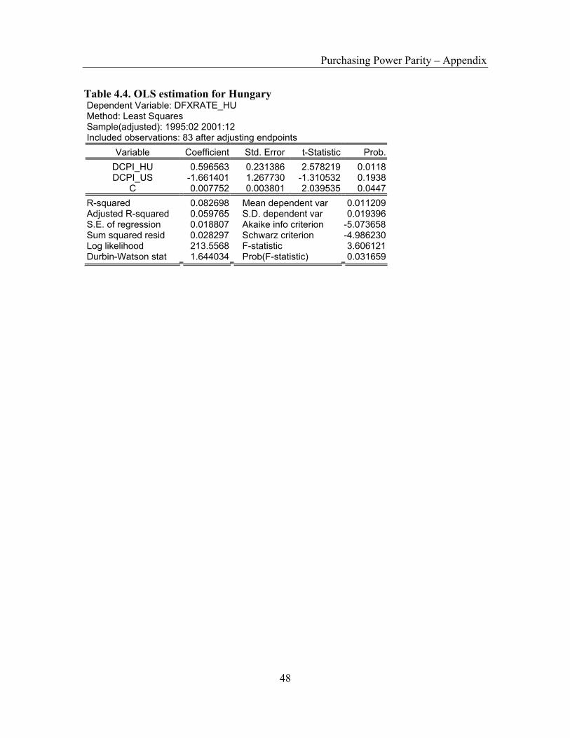
Table 4.4. OLS estimation for Hungary Dependent Variable: DFXRATE_HU Method: Least Squares Sample(adjusted): 1995:02 2001:12 Included observations: 83 after adjusting endpoints

Variable Coefficient Std. Error t-Statistic Prob. DCPI_HU 0.596563 0.231386 2.578219 0.0118DCPI_US -1.661401 1.267730 -1.310532 0.1938

C 0.007752 0.003801 2.039535 0.0447R-squared 0.082698 Mean dependent var 0.011209Adjusted R-squared 0.059765 S.D. dependent var 0.019396S.E. of regression 0.018807 Akaike info criterion -5.073658Sum squared resid 0.028297 Schwarz criterion -4.986230Log likelihood 213.5568 F-statistic 3.606121Durbin-Watson stat 1.644034 Prob(F-statistic) 0.031659

References

1. Arghyrou, M. G. (2000), “Exchange Rate Pegging: Credibility and Fundamentals.

Evidence from Greece”, Brunel University

2. Engel, C. and J. C. Morley (2001), “The Adjustment of Prices and the Adjustment

of the Exchange Rate”, working paper 8550, www.nber.org

3. Greene, W.H. (1997), “Econometric Analysis”, Prentice Hall International, Inc.,

New Jersey, 789-796

4. Levich, R. M. (1998), “International Financial Markets. Prices and Policies”,

McGraw-Hill Co., London, 98-124

5. Maddala, G. S. (1998), “Introduction to Econometrics”, MacMillan Publishing

Company, New York, 577-601

6. Nagayasu, J. (1998), “Does the Long-Run PPP Hypothesis Hold for Africa?:

Evidence from Panel Co-Integration Study”, working paper 123, www.imf.org

7. Razzaghipour, A., G. A. Fleming, and R. A. Heaney (2000), “Purchasing Power

Parity and Emerging South East Asian Nations”, working paper #00-07, The

Australian National University

8. Schreyer, P. and F. Koechlin (2002), “Purchasing Power Parities – measurement

and uses”, working paper no.3, www.oecd.org

9. Steindel, C. (1997), “Are There Good Alternatives to the CPI?”, Current Issues in

Economics and Finance, 3(6), Federal Reserve Bank of New York

10. Taylor, A. M. (2000), “A Century of Purchasing Power Parity”, working paper

8012, www.nber.org

11. www.bnro.ro - National Bank of Romania

12. www.cnb.cz - National Bank of Czech Republic

13. www.imf.org - International Monetary Fund

14. www.mnb.hu - National Bank of Hungary

15. www.nbp.pl - National Bank of Poland

purchasing power parity. a survey on east european

Documents