Purchasing power parity exchange rates from household survey data: India and Indonesia

Angus DeatonResearch Program in Development Studies

Princeton University

Jed FriedmanVivi AlatasWorld Bank

May, 2004

We are grateful to Bettina Aten, Ralph Bradley, Erwin Diewert, Jean Drèze, Alan Heston, DavidJohnson, Johan Mistaen, Martin Ravallion, and seminar participants at Princeton, the WorldBank, and the Bureau of Labor Statistics for help in the preparation of this paper. This work wassupported in part by the DEC data group of the World Bank.

1. Introduction and outline

Purchasing power parity (PPP) exchange rates are extensively used in international and

development economics. Originally developed by the International Price Comparison Project for

the Penn World Table (PWT), there are now a number of different variants, most notably by the

OECD, Eurostat and the World Bank. Although the formulas differ, all of these PPP estimates

are based on prices and quantities for each country. As is the case for domestic CPI calculations,

the prices are typically representative prices collected in sales outlets, while the quantities are

commodity or commodity-group-specific national aggregates. In consequence, although there

exist PPPs for different aggregates, such as GDP, investment, consumption, and some of its

components, there are no PPPs for particular socioeconomic groups, for example for regions of

countries, or for those in poverty. Furthermore, the specific choices of index number formulas is

influenced by the uses to which the index numbers are to be put, typically the construction of

national accounts in a common PPP currency. The lack of poverty-specific PPPs, in particular,

has been a criticism leveled against the World Bank’s global poverty estimates of the number of

people living below $1 or $2 a day in PPP dollars.

Existing PPP exchange rates have a number of more general deficiencies. There are strong

domestic constituencies that care about domestic prices, and particularly the CPI, so that most

countries devote adequate resources for accurate index-number construction. That is not the case

for international index numbers whose construction is often under-resourced, and thus subject to

measurement error. Indeed, the revision from the 1985-based consumption PPPs in PWT5.6 to

the 1993-based consumption PPPs calculated by the World Bank resulted in very large changes

in estimated headcount poverty rates for 1993, even for broad regions of the world, from 39.1

1

percent to 49.7 in sub-Saharan Africa, and from 23.5 percent to 15.3 percent in Latin America

and the Caribbean, Chen and Ravallion (2002). Even the substitution of the consumption PPP

from the PWT6.1 for the consumption PPP constructed by the World Bank (which involves a

change in index number formula, as well as in various imputation assumptions) would remove

100 million Indians from $1-a-day poverty.

There are also systematic errors of various kinds. Countries who participate in PPP

benchmarking exercises are not selected at random. China has never participated in such an

exercise, and India has not participated since 1985. PPPs for such cases are imputed by a mixture

of extrapolations from old PPPs using domestic price indexes and imputations from cross-

country regressions. Worse still, since the one of the main consumers of PPP numbers are

international financial institutions and aid agencies, there are incentives for some countries to

overstate their price levels in international units, and thus to understate their GDP in PPP terms.

And once a country has established a favorable PPP, it has further incentives not to cooperate

with further benchmarks.

In this paper, we present an alternative method for calculating PPP exchange rates for poor

and middle-income countries based on prices and weights obtained from household survey data.

In many (although not all) household consumption surveys, respondents are asked to provide

information on both the quantities and expenditures of a large number of commodities,

particularly for food, beverages, tobacco, and fuel, where quantities are readily defined. The unit

value, the ratio of expenditure to quantity, although not a price, is related to price, so that such

data, compared across countries, hold out the hope of constructing consumption PPPs for a

substantial share of household budgets. The consumption surveys provide a very large number of

2

unit-values; for example, the Indian survey used here, which is a random sample of the national

population, contains more than 3.7 million unit values. If these unit values can be shown to be

informative about market prices, the survey information is likely to be at least as reliable as

prices collected from outlets, and because it is immediately tied to purchases, is guaranteed to

generate representative unit values in a way that is difficult to guarantee using prices collected in

retail outlets. And because the surveys collect a wide range of household characteristics, it is

possible to calculate price indexes in which both the prices themselves and the weights are

tailored to represent specific groups of the population. Against these advantages of the survey

methodology must be weighed the fact that prices and unit values are not the same thing

(something we investigate below) and that there is only be partial coverage of consumption.

PPP index numbers have an important domestic, as well as international function. In large

countries, such as Brazil, China, India, and Indonesia, both prices and patterns of consumption

differ across regions and between the cities and the countryside. As a result, regional and spatial

price indexes play an important role in measuring spatial differences in levels of living. In India,

national poverty rates are calculated by aggregating up the results from state by state and sector

by sector estimates, with price indexes for each sector of each large state used to adjust what is,

in principle, a common poverty line. The construction of a consistent set of price indexes, over

time, states, and sectors, is a classic problem in multilateral price index construction, to which

PPPs are the solution. Yet no such price indexes have been calculated for India to date, nor as far

as we are aware, for any other large country.

In this paper we calculate consumption PPP exchange rates for India and Indonesia in 1999,

with particular attention to poverty-relevant rates. We also present a consistent set of PPP price

3

indexes for the urban and rural regions of the major states of India. The Indian results are

presented first. Because there is a common survey instrument covering the whole country, it is

straightforward to match commodities across space, so that when calculating “domestic” PPPs,

we can focus on the unit-value versus price issue, as well as the way that PPPs vary with level of

living, without being concerned with international comparability problems. The Indian results

are in line with previous work; food, beverages, and tobacco are about 15 to 20 percent more

expensive in urban than in rural areas. There are also variations in PPPs across states, as well as

across levels of living, for example, between the top and bottom quartiles of household per

capita consumption.

The comparison between India and Indonesia presents a number of challenges in matching

items across countries, because Indonesian consumption patterns and the survey design tailored

to them differ in major ways from Indian patterns. We explore a match based on identifying the

same commodities in both countries, as well as one based on the calorie content of number of

matched food groups. Our results appear to be robust to those choices, although the Indonesian/

Indian PPP exchange rate at the $1-a-day poverty line is a few points higher than a PPP

calculated for all households. Both of those rates are substantially (10 to 20 percent) lower than

the aggregate-weighted PPPs that result from following the current aggregate methodologies

used in PWT or by the World Bank. However, our major finding is that all of our rupiah to rupee

exchange rates are substantially (more than 50 percent) higher than the current PWT or World

Bank rates. Either Indonesia in 1999 was much poorer than it appears in standard tables, or India

in 1999-2000 is much better off. The latter is plausible, if only because no Indian benchmarking

has been done for almost 20 years, but our results would also be consistent with understatement

4

of the official consumer price index in Indonesia from 1995 through 1999, a period that includes

the Asian financial crisis.

2. Multilateral index numbers: theory

Purchasing power parity exchanges rates are examples of multilateral price indexes that use

price and quantity information to calculate price levels for a number of countries (states, or

regions) simultaneously. As with bilateral price indexes, there are a number of properties that

multilateral index numbers should ideally satisfy, and since these typically cannot all be satisfied

simultaneously, analysts are forced to choose guided by the purpose of the index. For n

countries, bilateral price indexes generate an n by n matrix of indexes. These price indexes

typically do not exhibit transitivity, so that the price index of country A with country B as base

will not generally equal the product of the price index of C with B as base and the index of A

with C as base. To satisfy transitivity, we need not a matrix of price comparisons, but an n

vector, defined up to scale, the elements of which are interpreted as the price levels of each

country. For practical reasons (on which more below), it is usual to assemble countries into

regional groupings, and to compute multilateral price indexes for all countries in the group, with

the groups linked to one another through one or more countries from each.

A useful starting point, which allows us also to establish notation, is to restate the standard

bilateral price index numbers. If indexes countries, and indexes

commodities, and and are the price and quantity of good n in country i in local currency,

then the Laspeyres (suffix L) and Paasche (suffix P) index numbers for country j relative to

country i, are

5

(1)

(2)

(3)

More immediately useful in the multilateral context are the Fisher Ideal (suffix F) and Törnqvist

(suffix T) index numbers

where is the share of the budget of good k in country i,

Unlike the Paasche and Laspeyres index, the Fisher and Törnqvist price indexes make symmetric

use of the weights from both countries in making the bilateral comparison between them. They

also satisfy the important “country reversal” test, that the price of i relative to j should be the

reciprocal of the price of j relative to i,

The PWT index numbers use the Geary-Khamis multilateral index, in which the goods from

each country are priced at a set of “world” prices and a system of Paasche price indexes formed

with aggregate quantities as weights. The Geary-Khamis price index for country i, is

implicitly defined by the two equations

6

(4)

(5)

where is the “world” price of commodity n, and is the aggregate consumption of

commodity n in country i. Equation (4) is a Paasche index, while equation (5) defines the world

price of each good as an aggregate-commodity weighted cross-country average of each country’s

price of the commodity expressed in PPP terms. Equations (4) and (5) can be solved iteratively,

or reformulated as an eigenvector problem, Diewert (1999), Balk (2001).

Because GK indexes are calculated from repricing individual commodities, they can readily

be applied to subcategories of consumption, or of GDP, and the PPP value of these subcategories

will add up to the totals. This additivity property is important for the construction of national

accounts, and is one of the reasons why the GK method is used in the construction of the PWT.

It is less important when our main concern is the construction of price indexes for comparing

levels of living. And as Diewert (1999) has shown, the additivity property is frequently in

conflict with other important desiderata for multilateral index numbers.

Because the world prices in (2) are constructed using aggregate quantities as weights, rich

country prices are overweighted relative to poor country prices, so that in a region containing

India, Japan, and Indonesia, for example, the Japanese prices would tend to dominate, especially

for items such as cars or consumer durables. Nuxoll (1994) calculated that the GK world prices

7

(6)

(7)

in the PWT are close to those of a country whose level of development is approximately that of

Hungary or Yugoslavia. For our current purpose, which is the comparison of one poor country or

region with another, using “Japanese” or even “Hungarian” prices as the standard has little to

recommend it. Even for a two country comparison, with no rich country included, the Geary-

Khamis index suffers from a related version of the same problem, which is that richer

households spend more and so are overweighted, both in the construction of the world prices

and in the Paasche index (4), which is a plutocratic index in the sense of Prais (1959).

The World Bank, OECD, and Eurostat PPPs are calculated according to the EKS formula,

Eltetö and Köves (1964), Szulc (1964), originally proposed by Gini (1924). This starts from the

two I by I matrices of bilateral Fisher indexes, although exactly the same procedure could be

applied to the Törnqvist indexes. The EKS price index for country i is defined (up to scale) by

The EKS index is most simply thought of as a transitive version of the system of bilateral Fisher

index numbers. Indeed it is readily shown that, up to scale, (6) is equivalent to the definition

so that transitivity is enforced by averaging the (log) Fisher indexes over all possible “bridge”

countries. Alternatively, the index can be derived as the least squares solution to selecting a

vector of country log price levels that are as close as possible to the logarithmic bilateral Fisher

indexes. Intuitively, (6) says that the (log) price level of country i is the average of its (log) price

levels using all other countries as base.

8

(8)

Another important multilateral method is the weighted country-product-dummy (WCPD)

method due to Prasada-Rao (1990), (2002). The logarithm of the price of commodity n in

country i is regressed on a set of commodity and country dummies using weighted least squares

with aggregate budget shares as weights; the estimated country dummies are then the logarithms

of the PPP index numbers. The regression can be written

where is the Kroenecker delta, equal to 1 if i=j and 0 otherwise, and the weights are given by

equation (3), and is defined as the coefficient on the jth dummy variable.

Interpreted as a model of prices, (8) assumes that, up to random noise, the structure of

relative prices is the same in all countries, which is clearly not true, and if true, would obviate

the need for index numbers. Instead, the regression should be interpreted as a device for

calculating the PPPs Intuitively, the structure of (8) is what we would like prices to satisfy

in order to calculate a consistent vector of country PPPs, and by forcing the approximation, with

deviations weighted by their importance in the aggregate budget as in (8), we obtain a useful set

of indexes. Rao (2002) has shown that (8) is the solution to a system of equations proposed by

Rao (1990) and which are similar to those satisfied by the Geary-Khamis index, but with budget

shares replacing quantities, and log prices replacing prices.

The weighted CPD index has the practical advantage that its estimation does not require that

all prices be observed in all countries, a requirement that is rarely met in practice, see Summers

(1973) who introduced the unweighted CPD in this context. It can also incorporate hedonic

information about the characteristics of goods, which is helpful when goods cannot be exactly

9

matched across countries, see Kokoski, Moulton, and Zieschang (1999). There are a number of

criteria by which these three multilateral index number formulas might be judged. In the spirit of

Fisher, Diewert (1987), (1999) and Balk (2001) have proposed a number of tests that reasonable

multilateral price indexes should satisfy. All three indexes used here satisfy a substantial number

of these tests, though none of them (nor any other known index) satisfies them all. The additivity

property of the GK index is satisfied neither by EKS nor by WCPD. Both EKS and WCPD have

a property that GK does not, which is that the price comparison between country i and country j

involves an averaging of weights from both countries. In EKS, the underlying Fisher (or possibly

Törnqvist) indexes are superlative index numbers in the sense of Diewert (1976), which means

that they are exact cost-of-living index numbers for some (common across countries) homothetic

utility function that is a flexible function form, meaning that it allows a fully general matrix of

price substitution effects. Diewert (2002) has also shown that, in the case of two countries, the

logarithm of the WCPD index is a weighted mean of the logarithms of the price relatives, where

the weights are the harmonic means of the budget shares. Such an average provides a second-

order local approximation to the Törnqvist price index which is itself superlative.

In the context of computing PPP price indexes across rich and poor countries, or even

between two poor countries or states of a single country with sharply different consumption

patterns, the assumption of common homothetic tastes is an extraordinarily unattractive one, so

that the argument that superlative indexes are consistent with such tastes carries little force. Even

so, there are compelling arguments within the PPP context for using superlative indexes, or

something close to them. As we shall see, both across the states of India, and between India and

Indonesia, there is a negative correlation between quantities and relative prices. This correlation

10

is doubtless partly a result of substitution in response to price differences, but it also reflects

long-standing differences in tastes. Whatever the reason, the Paasche price index will often be

much lower than the Laspeyres. Unlike the case of comparisons of prices over time, there is no

natural ordering that sets one situation as the base and the other as the comparison. Given this

lack of asymmetry, sensible bilateral comparisons must not depend on which country is chosen

as base, so that they must satisfy the country reversal test. Because the Paasche and Laspeyres

indexes do not satisfy the country reversal test, but rather the identity , a large

difference between the two indexes is simply another way of saying that both are far from

satisfying the country reversal test. Their geometric average, the Fisher index, satisfies country

reversal, as do all superlative indexes. Such arguments have been used by Diewert (2001) to

provide an elegant axiomatic argument for the use of superlative price indexes in all such

situations, without depending on the fact that such indexes are approximations to true cost-of-

living index numbers under rather specific assumptions.

All three indexes can be calculated from household survey data. The next section discusses

how we obtain the prices, and the aggregate quantities can be obtained from survey reports by

applying the survey inflation factors (inverse probabilities) to estimate population aggregates.

Beyond this, prices and aggregate quantities can be estimated for population subgroups, such as

those below or near the poverty line. Moreover, the surveys also allow us to use “democratic”

weights for the price indexes which avoid the plutocratic bias associated with aggregate

quantities, even aggregate quantities within subgroups. More specifically, the aggregate

Laspeyres index is

11

(9)

(10)

(11)

where h denotes a households, of which there are in country i’s population, is the share

of aggregate consumption of good n in total consumption of country i, The household

budget shares are household total expenditures are and are the plutocratic

budget shares, where each household’s budget share is weighted by its share of total national

expenditure. These plutocratic weights for the Laspeyres are unattractive for calculating real

living standards, even within population subgroups, and we shall typically replace (9) by its

“democratically” weighted counterpart, which is

where is the arithmetic population average of the household budget shares. The democratic

Paasche is defined in a parallel way, as the weighted harmonic mean of price relatives

These two democratic indexes satisfy the usual relationship that so that the

democratic Fisher index formed from them satisfies the country reversal test.

The democratic WCPD is calculated from regression (8) using the democratic budget shares

as weights, while the democratic EKS comes from (6) using the democratic Fisher indexes.

These are the indexes that we recommend for work on the measurement of living standards. For

comparison with PWT, we also calculate the GK index, but we use (4) and (5) directly, which

12

are the plutocratic indexes, again for maximum comparability with PWT.

3. Multilateral PPP indexes for India

In this section we use data from the Indian National Sample Survey (NSS) for 1999–2000 to

construct PPP price indexes for each sector of the 14 major states plus Delhi. State by sector

price indexes are used in India to construct state and sector specific poverty lines, on which state

and national poverty estimates are based, Government of India (1993). These poverty counts are

among the most closely watched statistics in India, and are used, in part, to determine the size of

anti-poverty transfers from the center to the states, for example through food subsidies. The

poverty statistics have also been the focus of a fierce debate on the extent to which poverty has

declined since India’s program of economic reforms since the early 1990s, see for example

Bhalla (2001), Sen (2000), Sundaram and Tendulkar (2003),and Deaton and Drèze (2001). One

thread in this debate has been the inadequacy of the state-specific price indexes that are implicit

in the government’s poverty lines.

3.1 Indian data and consumption patterns

Table 1 provides an overview of the data from the NSS sample. The survey collected data from a

sample of 71,382 rural and 48,919 urban households, of which 60,076 rural and 40,842 urban

households live in the 14 large states (and urban Delhi) that we analyze. Our multilateral system

contains 29 locations, the urban and rural sectors of 14 states, plus urban Delhi. The survey

asked respondents to report the total value, and for applicable goods, the quantity of household

consumption over both the last 30 and 7 days. The shorter reporting period was part of an

13

experiment in this survey, and we make no use of those numbers. Respondents are asked to

report whether their consumption came entirely from purchases, entirely from homegrown stock,

from both, or from gifts. We use only the former to calculate unit values, though in the

construction of budget shares or quantity weights, we use consumption from all sources. For the

food, beverages, tobacco, and fuels that we analyze, there are 167 commodities for which the

survey provides unit values. The sample that we use contains just 2.08 million rural and 1.80

million urban unit values, whose distribution over states is shown in the right-hand panels of

Table 1. Note that the ratio of the number of unit values to number of households is larger in

urban areas where a wider variety of goods is available.

Table 2 records, separately for rural and urban, the most important items of consumption

according to their (democratic average) share of the budget. Clearly, these rankings are arbitrary

because they depend on the degree of commodity disaggregation; for some items, such as

vegetables, a large number of commodities are distinguished (snake gourd, arum, radish, for

example), while for others, there is only a single item (rice, fish and seafood.) Nevertheless, the

table provides an indication of which unit values play the largest part in the analysis, as well as

showing some of the important differences between urban and rural consumers, as well as

between the North and South of the country.

Rice is important throughout India, more so in rural than in urban households, more so in the

south than the north, where wheat is the most important cereal. In general, the important

commodities are rice, wheat, milk, sugar, pulses (lentils), cooking oil, and fuel, although the

balance between the items, and the details, for example the type of cooking oil, vary from place

to place. In Kerala, rice is the basic staple, wheat is not consumed, fish is important, as are

14

coconuts and coconut oil. In Uttar Pradesh, wheat takes over from rice, though the latter is still

important, mutton and goat are eaten, not fish, pulses are extremely important, and mustard oil is

typically used for cooking. Throughout India, there are Public Distribution System (PDS) or

“fair price” shops, in which state governments sell staples at below market prices, most

importantly rice, wheat, sugar, and kerosene. The effectiveness and availability of the PDS

varies from state to state, and is particularly highly used in Kerala, as can be seen in the table. By

contrast, the PDS is less well-used in Uttar Pradesh, although more than 80 percent of

households by kerosene from the PDS, and 46 percent buy sugar. Given these marked difference

in consumption patterns between the two states, it would make little sense to price out the

Keralan bundle in Uttar Pradesh, or vice versa.

3.2 Unit values and prices in India

The most difficult issue in using unit values in price indexes is the extent to which unit values

are indeed useable as prices. Perhaps the main concern is quality variation. Even within a single

commodity, such as rice or sugar, there are quality variations, and it is not obvious how variation

in unit values across households, or across regions, is to be parsed into its quality and price

components. Deaton (1988, 1997, Chapter 5) has developed a framework in which each

commodity is seen as an aggregate of underlying commodities, and has defined index numbers

such that expenditure is the product of a quantity index, a price index, and a quality index. Unit

value is the product of the last two, neither of which is directly observed, although it is the price

component that we wish to include in the price indexes. In particular, we do not want to count

Delhi as more expensive than Bihar, simply because its inhabitants are richer, and on average

15

buy higher quality foods, or buy cigarettes instead of bidis.

Quality variation is less serious the finer is the classification of commodities, so that it is

important, when using unit values, to work with the maximum disaggregation available, rather

than with subgroups of goods, such as cereals, meats, or vegetables. Even so, and even with 167

commodities, goods are not homogeneous. For example, there are many varieties of rice, which

is one of our commodities, and rice in turn is much less heterogeneous than is the category “fish

and seafood,” which is a single group in India, although it is split into 32 categories in the

Indonesian survey that we use below. Even so, we shall argue that the quality component in the

unit values is likely to be relatively small.

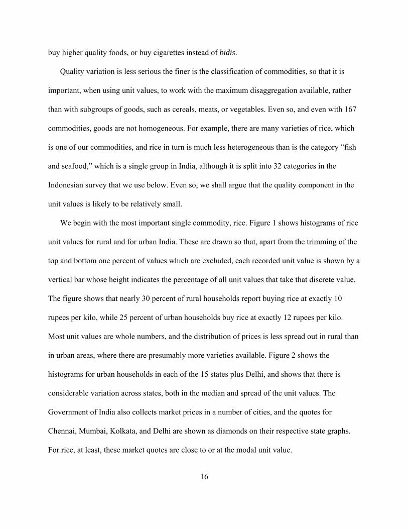
We begin with the most important single commodity, rice. Figure 1 shows histograms of rice

unit values for rural and for urban India. These are drawn so that, apart from the trimming of the

top and bottom one percent of values which are excluded, each recorded unit value is shown by a

vertical bar whose height indicates the percentage of all unit values that take that discrete value.

The figure shows that nearly 30 percent of rural households report buying rice at exactly 10

rupees per kilo, while 25 percent of urban households buy rice at exactly 12 rupees per kilo.

Most unit values are whole numbers, and the distribution of prices is less spread out in rural than

in urban areas, where there are presumably more varieties available. Figure 2 shows the

histograms for urban households in each of the 15 states plus Delhi, and shows that there is

considerable variation across states, both in the median and spread of the unit values. The

Government of India also collects market prices in a number of cities, and the quotes for

Chennai, Mumbai, Kolkata, and Delhi are shown as diamonds on their respective state graphs.

For rice, at least, these market quotes are close to or at the modal unit value.

16

We have constructed and examined graphs like Figures 1 through 3 for a large number of

commodities. Some of the unit values have more spread than does rice (e.g. cooked meals) and

some less (e.g. milk), and some about the same (wheat). The variation with quartiles of

household per capita total expenditure (Figure 3) is a greater for rice than for most commodities;

for example, for liquid milk, there is little or no variation in unit values across the quartiles of

PCE. For the few commodities where we have market prices, the match is as close as that shown

in Figure 2, with one interesting exception. The market price of milk in Mumbai in December

1999 in the official statistics was 20 rupees per liter. From the survey, the median unit value in

urban Maharashtra was 13.5 rupees, 20 rupees was at the 95th percentile, and only 268 out of the

4,593 urban households who bought milk reported paying 20 rupees or more. It is simply not

plausible that 20 rupees per liter was a representative price for milk in urban Maharashtra in this

period. This example is worth noting because it shows that data on market prices should not

automatically be treated as the gold standard. While such data are free of the problems that come

from unit values not being prices, they suffer from other deficiencies, in particular that they

come from a small number of outlets, whose selection into the sample of often not well

documented, and which may not be representative. In the case of milk in urban Maharashtra, we

are comparing a single price quote with 4,593 reported unit values, 931 of which are exactly at

14 rupees, and which show no sign of quality variation with total expenditure or other

socioeconomic characteristics.

Figure 4, which shows the distribution of urban unit values for wheat over states, shows a

negative correlation across states between unit values and consumption. In those northern states

where wheat is the staple, particularly Uttar Pradesh, Punjab, and Rajasthan, the unit values

17

cluster towards the bottom of the range, while in southern states where wheat is little consumed,

particularly Andhra Pradesh, Kerala, and Tamil Nadu, the unit values cluster at the top of the

range. Similar phenomena are common across the consumption basket, and are often more

extreme. For example, although mustard oil is the fourth most important item in the budget in

rural India (Table 2), with more than a half of households reporting purchases over the last

month, there are only 2 reported purchases in rural Kerala, 9 in rural Karnataka, 17 in rural

Tamil Nadu, and 22 in rural Maharashtra. These facts lend further credence to the supposition

that the unit values are closely related to prices. They also underline the dangers of attempting to

calculate price indexes by pricing out any single commodity bundle across states.

Table 3 further documents the spatial structure of unit values, as well as their relationship to

household characteristics. The first two columns, arranged in descending order of importance in

the budget, show the fraction of the variance in each unit value that is accounted for by its

between-state and between-district components; because districts are subunits of states, the

second column is always larger than the first. The third column shows the estimated fraction of

households in the population whose purchases are exactly at the median unit value for the state

in which they live, or if the median is not a whole number, are exactly equal to one of the whole

numbers on either side of the median. These numbers are averaged (without weights) over states.

The between-state component of the variance is never larger than a half (potatoes, PDS rice), and

for some commodities (mustard oil, arhar, LPG, and sugar) it is less than ten percent. The

between district variation is around 10 percent higher. We have no means of parsing the rest of

the variance into its other components, measurement error, local price variation, and variation in

unit values that has nothing to do with variation in prices.

18

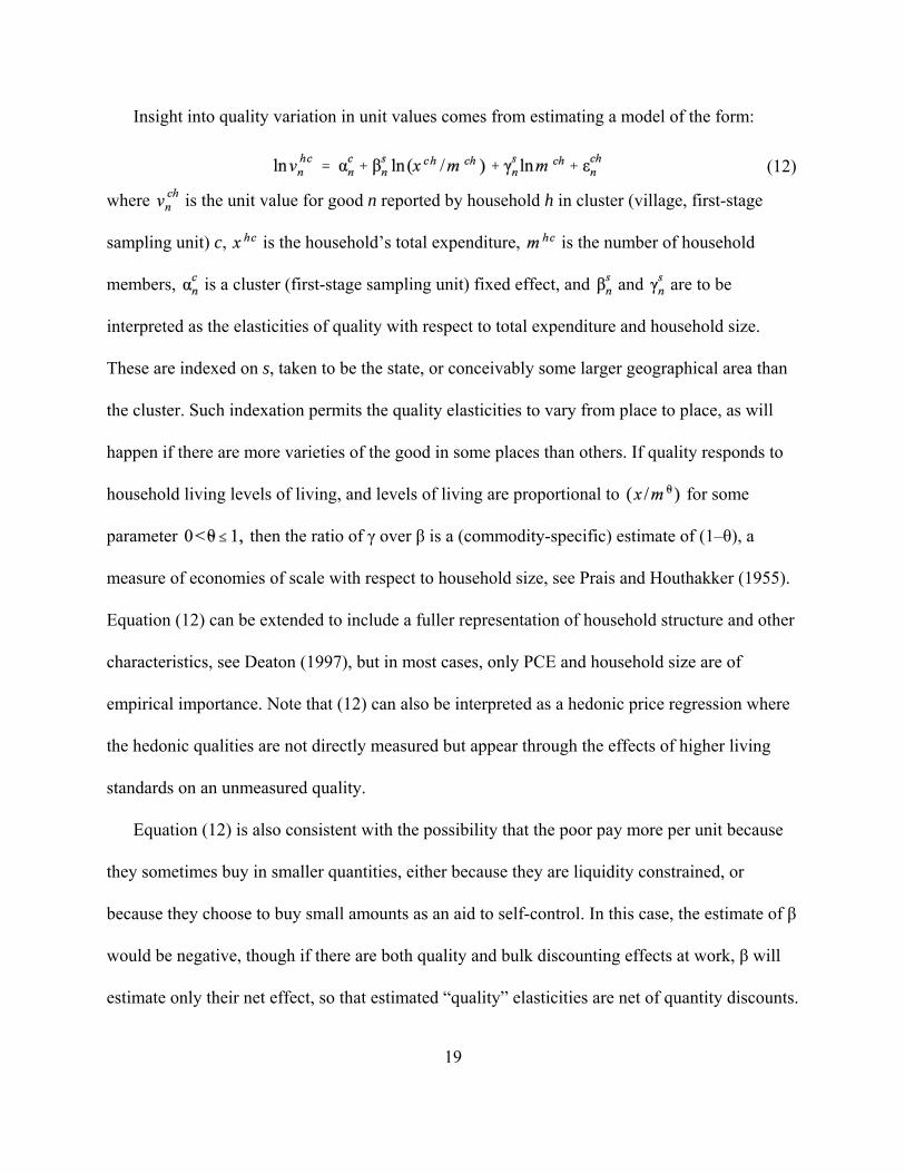
(12)

Insight into quality variation in unit values comes from estimating a model of the form:

where is the unit value for good n reported by household h in cluster (village, first-stage

sampling unit) c, is the household’s total expenditure, is the number of household

members, is a cluster (first-stage sampling unit) fixed effect, and and are to be

interpreted as the elasticities of quality with respect to total expenditure and household size.

These are indexed on s, taken to be the state, or conceivably some larger geographical area than

the cluster. Such indexation permits the quality elasticities to vary from place to place, as will

happen if there are more varieties of the good in some places than others. If quality responds to

household living levels of living, and levels of living are proportional to for some

parameter then the ratio of γ over β is a (commodity-specific) estimate of (1–θ), a

measure of economies of scale with respect to household size, see Prais and Houthakker (1955).

Equation (12) can be extended to include a fuller representation of household structure and other

characteristics, see Deaton (1997), but in most cases, only PCE and household size are of

empirical importance. Note that (12) can also be interpreted as a hedonic price regression where

the hedonic qualities are not directly measured but appear through the effects of higher living

standards on an unmeasured quality.

Equation (12) is also consistent with the possibility that the poor pay more per unit because

they sometimes buy in smaller quantities, either because they are liquidity constrained, or

because they choose to buy small amounts as an aid to self-control. In this case, the estimate of β

would be negative, though if there are both quality and bulk discounting effects at work, β will

estimate only their net effect, so that estimated “quality” elasticities are net of quantity discounts.

19

We are skeptical of the idea that poor people consistently and over long periods pay higher

prices than necessary for basic staples, such as wheat, rice, or milk, though there may be such

effects for infrequently purchased items, or for commodities subject to self-control problems,

such as tobacco, or even tea. Also potentially important is the inability of some poor households

to pay the fixed costs associated with access to consumption technologies with lower marginal

costs, so that they are forced, for example, to use batteries instead of mains electricity, or to pay

bus fares instead of riding a bicycle. But we of no methodology that could incorporate these

effects into a price index.

The results from estimating equation (12) are shown in the last two columns of Table3. The

elasticities of unit value with respect to total expenditure tend to be higher in urban areas,

presumably because more variety is available. The expenditure (and household size) elasticities

of quality vary as is to be expected with the degree of heterogeneity of the good. Cooked meals

and fish and seafood have amongst the highest quality elasticities, and sugar and kerosene

amongst the lowest. The most important commodities, rice, milk, and wheat, have quality

elasticities between 0.057 (rural milk) and 0.232 (urban rice). For our current purposes, it would

be better if these elasticities were close to zero, which would be consistent with the

disaggregation being fine enough to remove quality effects. Even so, the difference between the

10th and 90th percentiles of log PCE is 1.11 among rural households, and 1.46 among urban

households, so that the expected unit value of rice at the 90th percentile is estimated to be 17 (34)

percent higher than at the 10th percentile in rural (urban) households. This variation, which is

larger for rice than for any other important commodity, needs to be borne in mind when

considering unit value methods as compared to other techniques for PPP calculation. Note that

20

the table shows no evidence that the poor pay less; of the goods shown, only sugar and mustard

oil have negative elasticities, and both are tiny. While it is possible that the typical small

elasticities for most commodities are the result of offsetting effects from quantity discounts and

quality upgrading, that this should happen for nearly every commodity is unlikely. A more

straightforward interpretation is that systematic bulk discounting is rare, and that quality effects

are almost always present, but small, except in those cases where the disaggregation is clearly

insufficient to eliminate heterogeneity.

At first sight, a promising method for dealing with heterogeneity is to follow Kokoski,

Moulton, and Zieschang (2001) and use (12) to “correct” the prices and thus to the incorporate

the hedonic effects into the price indexes. But the analogy does not go through to this case,

because we have no direct measure of the quality of each good. Without that, the parameters in

(12) could be used to calculate quality-corrected prices by recalculating prices at some common

values of PCE and household size. But this proposal founders on the fact that the β and η

parameters vary across states and sectors (results not shown.) Suppose, for example, that in rural

villages only one variety of rice is available, while in the cities, there are several. Our estimate of

β will be zero among the rural households, and positive among the urban households. We could

indeed compare prices paid at a common level of PCE, but the urban variety implicitly identified

could be of higher or lower quality than the single rural variety. Without direct measurement of

quality, the regression approach cannot control for product quality indirectly.

Note finally that comparison of the last two columns of Table 3 shows that the results are at

least roughly consistent with an estimate of θ around one-half. Prais and Houthakker’s method

for measuring economies of scale clearly does not generate the paradoxes that come from a

21

direct examination of what happens to food consumption per capita as household size increases,

see Deaton and Paxson (1997).

3.3 Multilateral indexes for India

The indexes presented in this section are based on 167 commodities in total, covering food,

beverages, tobacco, and fuels. These are observed for the rural and urban sectors of each of the

14 major states, plus urban Delhi, giving 29 “places” in all. Not all goods are reported to be

purchased in all places. For the budget shares, this is not an issue; when a good is not purchased,

it has a budget share of zero. However, we observe a unit value only when a commodity is

purchased, so we need a procedure for dealing with missing values, at least for the EKS indexes,

although for the weighted-CPD indexes, the regressions can be run with the missing values

included. Rather than rely on this, and to ensure comparability between the different indexes, we

have imputed missing unit values using an unweighted CPD scheme, in which the logarithms of

unit values are regressed on a set of item and state/sector dummies. Of the total of 4,785

price/quantity pairs (165 commodities in 29 state/sectors), 135 are imputed in this way. Unlike

the procedures in the earlier related work in Deaton and Tarozzi (2000) and in Deaton (2003),

we have made no attempt to inspect and edit individual unit values, for example to remove

outliers, or to eliminate cases where there are only a few purchases of a commodity in a

particular location. The procedure that we are documenting is therefore a largely mechanical

one, which would surely be the case if it were routinely implemented. Because indexes (and

especially multilateral indexes) are averages over many observations, there is some inbuilt

protection against outliers, and we provide more by examining a number of different indexes.

22

Our first set of estimates, reported in the first two columns of Table 4, come from combining

the mean budget shares and median unit value for each place. It is important that the budget

shares add up to unity (at least over the whole budget), and adding-up is preserved by using

means. In addition, because each budget shares lies between 0 and 1, they are less affected by

outliers than are the unit values. By contrast, the distributions of unit values often have long right

tails consisting largely of measurement errors, against which the use of medians affords some

protection. When computing the summary statistics, budget shares are weighted by the number

of people they represent, which is the product of the survey inflation factor and the number of

people in the household, while the unit values, which represent household purchases, are

weighted by the household weights. The weighted-CPD indexes are calculated by exponentiating

the estimated state/sector dummies in a mean budget share-weighted regression of log median

unit values on place and item dummies. As in all the calculations, rural Andhra Pradesh is the

base. The EKS index starts from 29 by 29 matrices of Paasche and Laspeyres indexes, which are

used to calculate a matrix of Fisher indexes. The averages of the columns of the logarithm of the

Fisher indexes are the logarithms of the EKS multilateral index.

The correlation between the EKS and CPD indexes is 0.957, so that there is little to choose

between them in practice. Rural Kerala has the highest prices in rural India, more than 20

percent higher than rural Andhra Pradesh. Urban Delhi is the most expensive place, although

urban Gujarat and Maharashtra are only a point or two behind. The rural prices are similar

(ρ=0.87) to the unilateral price indexes in Deaton (2003), used in the poverty calculations in

Deaton and Drèze (2003), and the rural/urban price difference is close to the 15 percent in this

earlier work, as well as in previous Indian literature.

23

The NSS surveys distinguish purchases from the Public Distribution System (PDS) from

those from other sources, at least for the four important commodities, rice, wheat, sugar, and

kerosene. In the first two columns of Table 4, we have followed the NSS, treating (for example)

rice from the PDS and rice from the “free” market as separate commodities. Such a methodology

will generally fail to reflect the reduction in prices brought about by the PDS in areas where it is

effective. Suppose, for example, that rice is sold in the PDS shops at 10 rupees per kilo and at 13

rupees in the free market. In area one, the PDS is ineffective, there are few stores, and they are

rarely open. In area two, the two prices are the same as in area one, but households get their full

PDS rations. The price relatives between the two areas are unity for both “types” of rice, so that

all rice price indexes between the two areas are unity, so that they do not capture the fact that

rice is cheaper in area two. One way to handle this issue is by using only the non-PDS price, and

assigning to each household the value of its infra-marginal subsidy through the PDS. In a

poverty calculation, for example, household total expenditures would be adjusted upward

relatively in those areas where the PDS is effective, and its effects on reducing poverty would be

accounted for. However, given that this is not done in practice, there is a good deal to be said for

adjusting the price indexes to capture the subsidies.

We make the PDS correction by combining the two kinds of rice, wheat, sugar, and kerosene

into four commodities, whose budget shares are the sums of the PDS and non-PDS budget

shares, and whose “price” is the budget-share weighted average of the two (median) unit values

in each place. We then calculate the CPD and EKS indexes as before, and the result is shown in

the third and fourth columns of Table 4. Not surprisingly, the major (and almost only)

beneficiary of the change is Kerala, whose rural price index falls from 1.24 to 1.15 (1.22 to 1.16

24

by EKS) and whose urban price index falls from 1.27 to 1.19 (1.28 to 1.22, EKS). The other

states are barely affected. All further calculations make this correction for the PDS goods.

The remainder of Table 4 explores the effects on the index numbers of a quality adjustment

that is designed to eliminate the differences across areas that come from the effects of interarea

differences in incomes and family composition on the average of reported unit values. We use a

modified version of the procedure adopted by Condoo, Majumder, and Ray (2002) in which the

logarithm of the unit value of each good is regressed on a set of area dummies, on the logarithm

of household per capita expenditure, and on the logarithm of household size, see also (10) above.

The regression coefficients are then used to predict the area mean log prices using the All India

(urban and rural separately) means for the logarithms of per capita expenditure and household

size. In this way, we net out the influence of pce and household size across states within each

sector. The results of this procedure differ from earlier results not only through the quality

adjustments, but also because we are no longer using the median unit values. To isolate the

quality effects, we first run the regressions with only the area dummies, so that the area medians

of unit values are replaced by the exponentiated log means. These results are reported in

columns five and six, and are once again very close to those in previous columns. (This is also a

useful check on the robustness of the results in the presence of outliers and measurement error.)

The CPD indexes in columns 3 and 5 have a correlation coefficient of 0.981, and the EKS

indexes in columns 4 and 6 a correlation of 0.963. We can therefore be confident that the final

results, in columns 7 and 8, differ from the earlier ones because of the quality correction itself,

rather than the methodology used to make it.

The two quality corrected indexes differ between themselves rather more than do the

25

previous indexes, but they both differ more from the uncorrected indexes. For the rural areas, the

change that comes out in both indexes is again for Kerala, where there is an almost ten point

reduction in the index. In the urban sector, Bihar and Orissa, two of the poorest states, have their

price indexes revised upwards. Perhaps more notable than the state differences is the fact that the

quality corrections pull the price indexes together within each sector. For example, the quality

correction reduces the standard deviation of the CPD index from 6.2 to 4.9 percent across rural

states, and from 7.8 to 7.1 percent across urban states. Although the corrected indexes are still

well-correlated with the uncorrected indexes (col. 5 and 6 are correlated 0.89 rural and 0.88

urban), it would be foolhardy to claim that the corrections can fully capture quality variations

across states. We do not have direct measures of quality for any of these goods, and the

identification of the quality effects here rests on the (almost certainly false) assumption that the

effects of income and household size on unit values are the same in all areas. Indeed, faced with

these difficulties, it would be hard to mount a convincing case against the once standard

procedure of using the same poverty line for all households in India, differentiating only by

urban and rural sectors, and not within states.

All of the price indexes so far have used averaged data, and are therefore arguably

inappropriate for poverty work. In Table 5 we take up this challenge, experimenting with the use

of different weighting schemes and different prices for different parts of the distribution of living

standards. These numbers are calculated by splitting up Indian households into four quartiles of

per capita household total expenditure, and then recalculating mean budget shares and median

unit values for each area within each quartile. We experiment with schemes in which only the

weights vary by quartiles, using the same overall median unit values for all the quartiles, as well

26

as with schemes in which both the weights and the unit values are quartile specific. The former

is of interest because it is close to current procedures in which price information is collected in

shops and markets, not from households, but where weighting adjustments can be made to tailor

indexes to particular groups, such as those close to the poverty line. It would also be appropriate

if we believed that most of the variation in unit values within states comes from quality

differences, not from genuine differences in price. The second method, using quartile specific

unit values, allows for price differences across the distribution of per capita income, but is also

contaminated by quality effects to an unknown extent.

Table 5 shows the CPD indexes; the EKS indexes are similar enough to make it unnecessary

to report them. Column 1 labeled (0,0) repeats column 3 of Table 4, and uses the overall mean

weights (labeled 0) and the overall median unit values (labeled 0). Other columns are labeled by

the pair (x, y) where x denotes the quartile of the weights, and y denoted the quartile of the unit

values. Columns 2 through 5 all use the overall medians of the unit values, and differ only in

their weights. Columns 6 through 9 allow both weights and unit values to vary across the

quartiles.

Varying the weights alone makes little difference to these price indexes. Columns 2 through

5 are correlated at 0.97 or better, and even within sectors, the lowest correlation is 0.935. As is to

be expected, the correlations are higher between adjacent quartiles, and lowest between the first

and the fourth. But the differences are always small, so that weighting, by itself, is almost

certainly less important than other issues, such as quality adjustment or the proper treatment of

commodities sold through the PDS. Use of quartile-specific unit values makes a somewhat larger

difference. Once again, the correlations fall as the quartiles move further apart, but the

27

correlations are substantially lower than when only weights were varied. For example, for rural

states, the interstate correlation coefficient of the price indexes for the bottom quartile are 0.81

with the second quartile, 0.80 with the third quartile, and only 0.77 with the top quartile. The

corresponding urban figures are 0.95, 0.92, 0.77. The bottom quartile indexes are correlated at

0.83 and 0.86 with the uncorrected indexes that take no account of distribution. We suspect that

even these adjustments for distribution are relatively unimportant compared with other issues.

4. PPP exchange rates for India versus Indonesia

We now carry forward the Indian data and match it with data from the 1999 SUSENAS

household survey from Indonesia in order to calculate a purchasing power parity (PPP) exchange

rate between the two countries. A number of PPP exchange rates for the two countries are

available from standard sources. The Penn World Table has no direct bilateral comparison

between India and Indonesia, but yields a 1999 consumption PPP (calculated indirectly by

comparing the (GK-based) dollar PPPs for the two countries) was 165.2 rupiah per rupee. The

World Bank’s poverty monitoring website also gives (EKS based) US dollar PPPs for 1993.

Updating this for relative changes in consumer prices in the two countries gives a consumption

PPP of 140.0 rupiah per rupee, considerably lower than the PWT estimate. In consequence, if the

World Bank had used the rate from the Penn World Table instead of its own in its latest global

poverty estimates, either its local currency Indonesian poverty line would have been higher or its

local currency Indian poverty line would have been lower, and there would have been more

Indonesians relative to Indians in the global poverty counts. The foreign exchange rate between

the two countries averaged 182.42 rupiah to the rupee in 1999. According to the PWT,

28

Indonesia’s 1999 GDP per head was about 50 percent higher than India’s in PPP terms, or only a

little more than a third higher ((1.5 x (165.2/182.4))–1) in foreign exchange terms. If it is

generally true that PPP conversions bring measured GDP closer together than do foreign

exchange rate conversions, both the PWT and World Bank PPPs are on the “wrong” side of the

foreign exchange rate.

Because the consumption patterns in the two countries are quite different, our comparison

between India and Indonesia proceeds along different lines from our interstate and intersectoral

comparisons within India. Given that the survey instruments are different, it is a challenge to

match commodities between the two countries, and there are several important commodities in

each country that have no match in the other. In consequence, it makes little sense to construct a

single set of multilateral indexes that cover, for example, the provinces of Indonesia together

with the states of India. A better procedure is to construct a single bilateral comparison between

Indonesia and India, using the limited set of matching goods, and to do the internal comparisons

separately using the full range of goods in each survey, as we did for India in Section 3 above.

Our main focus here is on a PPP that compares rural Indonesia with rural India, although we will

also consider the four “country” multilateral comparison that including the urban and rural

sectors of each country. Another possibility, modeled on the way that the PWT works

internationally, would be to calculate internal multilateral comparisons for both countries, and

then to select one or more “bridge” states in each countries whose consumption and price

structures are as similar as possible.

29

4.1 The 1999 Susenas survey and matching commodities

The 1999 Susenas survey was conducted in the first two months of the year and collected

detailed consumption information for households in every Indonesian province except the then

province of East Timor. A total of 61,483 households were surveyed, 25,513 in urban areas and

35,970 in rural, and each household was asked about the consumption of 214 food commodities

over the past week, as well as the monthly consumption of 8 utilities such as electricity and

kerosene (petrol). As a result, Susenas contains 873,932 unit value observations for rural

households and 829,903 for urban households. As in India, the higher ratio of unit values per

household in urban areas than rural reflects the availability of a greater number of goods in those

areas. The Susenas surveys, like the NSS, distinguish between the consumption of goods

purchased in the market and those that have either been produced by, or gifted to, the household.

Since the method by which the surveys value self-produced goods is not transparent, we exclude

self-produced or gifted consumption when determining the median unit value for each good (but

include them when calculating the budget share).

Table 6 presents an overview of the Susenas consumption data. It lists the 20 commodities

with the largest average budget shares; because the comparison with India will not involve the

provinces, we present the data for the whole country, disaggregated only by rural and urban. As

in India, the single most important commodity in household consumption is rice, although

budget shares are substantially higher than in India. The consumption of rice is universal, with

99 percent of all households reporting consumption in the week prior to survey. The commodity

with the next largest budget share is filtered clove cigarettes, and when combined with unfiltered

clove cigarettes, the average budget share of cigarettes is nearly 5 percent. Prepared foods also

30

constitute an important general consumption category, in contrast with India, where relatively

little is spent. Susenas divides prepared foods into twenty distinct categories, and the three most

common categories are included in Table 6: rice with side dish (nasi rames), meat soup with

noodles or fried noodles (mie bakso or mie goreng), and fried food (typically tofu). Fresh and

preserved seafood is also an important consumption category, with 6.3 percent of rural

household budgets spent on this category. However since Susenas distinguishes among 32

seafood categories (such as fresh tuna or preserved shrimp), no single one category qualifies

among the top twenty listed.

To assess the spatial structure of the unit value data, we show the fraction of variance in the

unit values of each good that is accounted for by between-province and between-district

components. The between province component of the variance is almost never larger than a

third, with the exception of coconuts and the rice-with-side-dish category of prepared foods. The

between district component of variance is frequently twice as great as the between province

component. Overall, the amount of the variance accounted by province and district dummies is

roughly similar to that for India, as is the percentage of households consuming at median unit

values. The estimated quality elasticities (of unit values to household per capita expenditures) in

Table 6 are of much the same magnitude as those for India in Table 3, and the vast majority are

under 0.1. The goods with the highest elasticities tend to be the relatively heterogeneous

categories of prepared foods and cigarettes—cigarettes are one of the few goods listed in Table 6

that are sold under distinct brands, and the categories of prepared foods (rice with side dish, meat

soup with noodles, and fried food) are some of the most widely defined and heterogeneous

31

categories in the table. As is the case with the Indian data, the highest quality elasticities tend to

be in urban areas where the variety of goods available is likely to be greater.

To calculate PPP exchange rates we must match commodities across the two surveys. We

investigate two ways of matching; by a direct comparison of commodities that are the same in

each country, and by comparing broad food groups based on the caloric content of each. The

direct approach involves a one-to-one matching of goods in both surveys, such as sugar with

sugar or cabbage with cabbage, or of more aggregate goods that have a different number of

constituent goods in each survey. The relatively broad category of fish and prawns consists of 19

distinct Indonesian goods that fall under the fresh seafood category while the Indian data has

simply one category. Rice is only one good in the Indonesian data but the Indian data

distinguishes between PDS and non-PDS rice. In these cases, budget shares are summed over the

detailed goods, and median unit values are combined using budget shares as weights.

There are 62 commodity categories that can be directly matched between the Indian and

Indonesian surveys. In most cases these are individual items that match one for one between the

two surveys although there are a few cases where the detail is higher in one country than the

other. All told, 88 individual goods from the Indonesian survey and 71 goods from the Indian

survey are involved in the direct matching scheme. In a few cases, where the reference units

differ across surveys, we have made arbitrary assumptions that, while inaccurate to some extent,

are likely better than dropping the commodity from the analysis. For example we have assumed

that, on average, an Indian pineapple weighs 0.9 kg and an Indonesian egg weighs 0.0571 kg.

The 62 matched categories cover 47.9 (45.0) percent of the total household budget in rural

(urban) India and 53.1 (43.0) percent in rural (urban) Indonesia.

32

Table 7 shows a selection of the most important (and some less important) goods that can be

matched, together with their average budget shares in the rural sectors of the two countries, and

the commodity-specific purchasing power parity exchange rate, calculated as the ratio of the

median unit values in the two countries. The table shows the overwhelming importance of rice

for the calculation of the PPP; it accounts for more than 15 percent of the budget in India and 24

percent in Indonesia. Given that we cover only about half the total budget, rice accounts for 32

percent of the matched budget in India, and 45 percent in Indonesia. No other commodity is

close to as important and the rice-specific PPP of 266 rupiah to the rupee (if we include

subsidized rice from the PDS, or 250 rupiah per rupee if we do not) takes us a long way towards

the final consumption PPP. As we shall see, the difference between the PDS and the non-PDS

price of rice also has a substantial effect on the overall PPP, paralleling our earlier discussion for

the domestic Indian indexes.

Sugar and kerosene are two other goods that are important in both countries. The sugar PPP

is close to the rice PPP, but the kerosene-specific exchange rate is only 92 rupiah per rupee.

Kerosene, like other oil based fuels, are sold at substantially less than world prices in Indonesia.

The two sets of policies, low staples prices through the PDS in India and low fuel prices in

Indonesia, each have a substantial influence on the consumption PPP between the two countries.

For other commodities, the most notable feature of the table is the sharp difference in the

consumption pattern across the two countries. Wheat is second in importance only to rice in

India, but represents only 0.1 percent of the budget in Indonesia. Milk, potatoes, and tea are

important in India but much less so in Indonesia, and the opposite is the case for coconut,

cigarettes, and prepared food.

33

4.2 PPP rates for Indonesia versus India

Table 8 presents the bilateral price indexes or PPP exchange rates for rural Indonesia in terms of

rural India. The Laspeyres index is 39 percent higher than the Paasche, reflecting the differences

in consumption patterns and the negative association between consumption and price. The Fisher

(EKS) index is 233.3, which is close to both the weighted CPD index, which is 233.8, as well as

the Törnqvist index, which is 230.5. All of these rates are substantially higher than both the

World Bank and PWT rates, as well as the foreign exchange rate, implying that either Indian

households are better-off or Indonesian households worse-off (or both) than is typically

recognized. The table also shows what happens if we recalculate the index dropping the fuels or

dropping the PDS goods, using only the non-PDS prices. If we use the Fisher (EKS) index for

comparisons, the cheap fuel policy in Indonesia reduced the consumption PPP by 3.6 percent,

while the cheap food policy in India increases the consumption PPP by 3.7 percent.

We have explored a number of variants of these basic results. In an attempt to increase the

coverage of our match, we have followed an alternative construction that, for the foods, is based

on the price per calorie of 14 distinct groups. The idea here is not to compare the cost of a calorie

across the countries, a measure that would be contaminated by different choices over food

groups with widely different costs per calorie. Instead, we treat calories from each of the 14 food

groups as different goods, calories from cereals are different from calories from pulses, or from

seafood, which recognizes that each of the groups has important characteristics other than calorie

content that need to be recognized in calculating the PPP. We also include the non-food goods,

such as tobacco and fuels, in exactly the same way as in the previous comparisons. But the use of

calories allows us to include all of the foods within each group in each country even when

34

specific goods in each group cannot be matched directly. This allows us to match at the

functional group level such important cases as legumes, which take the form of lentils in India,

but appear as tofu in Indonesia.

Table 9 lists the fourteen food groups, together with their average budget shares for each

country, the local (median) cost per calorie, and the group-specific PPPs. These vary from 83 for

meat, which is relatively expensive in India, to 562 for vegetables, which are relatively

expensive in Indonesia. The case of fish is anomalous because it has a high commodity specific

PPP, although it is consumed more heavily in Indonesia. Note also that the commodity specific

PPP for fish from the calorie match, 507, is much higher than that from the commodity match,

which is 191 (Table 7.) Some of this difference comes from the inclusion of the calorie-poor

dried fish in the calorie match, but it should also be noted that these calorie equivalents are far

from straightforward to estimate—for example, they depend on how foods are prepared—and as

such, are subject to measurement error. The grouping procedure raises the coverage of the

budget to 57.4 (49.4) percent for rural (urban) India, and 63.1 (54.3) for rural Indonesia. The

PPPs calculated from those groups, together with the non-foods, are given in Table 10. These are

slightly higher than those reported from the commodity by commodity match, although only by

1.1 percent in the case of the Fisher (EKS) PPP index.

We have also included the urban sectors of both countries and calculated the multilateral

indexes for the four sectors using both the calorie- and commodity-match methods. These results

are given in Table 12. The rural to rural PPPs in the multilateral comparisons are very close to

those from the bilateral comparisons, and provide no reason to revise earlier impressions. Once

35

again, urban India is 15 to 21 percent more expensive than rural India, although the difference is

smaller in Indonesia, with urban prices only 7 to 10 percent higher than rural prices.

All of the PPPs calculated so far are close to one another, and lie in the range of 230 to 250

rupiah to the rupee, a range far in excess of the numbers in current use, more than 70 percent

larger than the World Bank consumption PPP, and more then 40 percent larger than the PWT

consumption PPP. Although the World Bank number is an EKS index, the PPP from the PWT is

calculated using the GK method, and both use aggregate weights, so that they are plutocratic, not

democratic indexes. We have calculated the plutocratic version of the EKS index for the bilateral

comparison between the two rural sectors, as well as the GK index, which also depends on the

relative sizes of the Indian and Indonesian economies. The Fisher (EKS) bilateral index is 243

rupiah per rupee, which is within the range of the other results, but the GK index is 257 rupiah

per rupee, which is the largest value of any so far considered. But these figures do nothing to

resolve the differences between our results and the other estimates.

4.3 Poverty-specific PPP-rates

All of the Indonesian to Indian PPPs presented so far use weights that are averaged over all

consumers, rather than being specifically tailored to the expenditure patterns of the poor. When

we are using an international poverty line, such as the World Bank’s $1 or $2 per person per day,

which is itself denominated in purchasing power-parity terms, poverty-specific PPPs need to be

calculated simultaneously with the poverty lines that depend on them. In this paper, we hold

fixed the official All Indian rural poverty line for 1999–2000, which is 327.56 rupees per person

per day. (If it were to be established that it is the Indian dollar PPP that is incorrect and the

36

(13)

Indonesian one correct, this would not be the obvious way to proceed.) We start from some

guess for the poverty-specific PPP between rural Indonesia and rural India, such as the Fisher

bilateral index already calculated, and use it to set up a first-round estimate of the comparable

Indonesian poverty line. We then calculate a PPP for the poor based on median unit values and

mean budget shares for households at or near the two poverty lines. This new PPP is used to

redefine the Indonesian poverty line, and thus to obtain a new estimate of the poverty-specific

PPP, and so on until the process converges.

The computation also requires some definition of which households are to be considered “at

or near” the poverty line, and we do this by weighting households according to their closeness to

the poverty line, and calculating weighted budget shares and unit values. More formally, if z is

the logarithm of the poverty line, and x is the logarithm of household per capita total

expenditure, a household with x is receives a weight proportional to ω defined by

if x is within h of z, and 0 otherwise. Equation (13) is a biweight kernel weighting function,

which declines monotonically with distance from the poverty line, and is zero once household

per capita expenditure is more than from the poverty line. The quantity h, measured in units

of log pce, is a bandwidth; for small values of h, all of the households are close to the poverty

line, but there are relatively few of them, while for large values, more households are included in

the calculation, at the potential risk of irrelevance. We experimented with bandwidths of 0.125,

0.25, 0.5, and 1.0.

37

For the Fisher (EKS) index using the commodity-match, this procedure always converged

within ten iterations, and the rural to rural PPPs (with associated bandwidth) were 238.2 (0.125),

239.8 (0.25), 238.2 (0.5), and 236.8 (1.0). Although these estimates are a few points higher than

the corresponding EKS index using the average budget shares (233.3), the difference is

insignificant relative to the general range of uncertainty of the calculations in general. This

conclusion is likely to be sensitive to the fact that our PPP index covers only food, tobacco, and

fuels. These items are relatively important in the budgets of the poor, so that if the PPP for other

items is differs from that for food, tobacco, and fuels, the consumption PPP for the poor is will

also likely differ from that of the all consumers taken together.

5. Conclusions

In this paper we have estimated multilateral price indexes for the large states and sectors of

India, as well as price indexes that compare Indonesia and India. Unlike most previous PPP

calculations, our estimates are based on household survey data. For India, our multilateral results

are not very different from previous estimates of intersectoral and interstate price differences,

although they have the additional advantage of being fully transitive. For the Indonesian to

Indian comparison, matters are very different, and our PPPs differ very substantially from those

in current use, whether the World Bank’s or Penn World Table estimates of the consumption

PPP. If our numbers were to be confirmed, either Indian households are a good deal richer or

Indonesian households a good deal poorer than is commonly supposed, or both, and there should

be more Indonesians and fewer Indians in the global poverty counts.

38

What are the possible reasons for the discrepancies? There are several possibilities, the most

important of which we list here:

(1) The Indian NSS data come from the calendar year 1999–2000, while the Indonesian Susenas

data were collected in January and February 1999. As a result, our PPP comparison relates to

those two time periods, whereas the World Bank, Penn World Tables, and exchange rate

conversions relate to a comparison of the two countries in the calendar year 1999. Prices were

quite stable in India in 1999–2000, and the consumer price index for agricultural laborers (the

usual price index for rural India) was only 1.6 percent higher for 1999–2000 than for calendar

1999. However, the Indonesian situation is quite different. Prices reached their post-crisis high in

January and February of 1999, so that, for example, the price of rice in January and February

was 8 percent higher than it was for the year as a whole. However, the CPI as a whole was only

1.5 percent higher in January and February than for the year as a whole, and its food component,

which is perhaps the nearest comparison for our index, 5.2 percent higher. Adjustment to a 1999

calendar year would lower our estimates by around 6.8 percent (5.2 plus 1.6), which is small

compared to the discrepancy.

(2) There is no up-to-date benchmark for India, which last cooperated fully in the international

pricing exercise in 1985. In consequence the Indian PPP in the PWT is computed by a mixture of

extrapolation using the CPI (75 per cent of the weight) and a short-cut regression estimate based

on cross-country comparisons of PPPs at different levels of development (25 percent). If the

Indian PPP in US dollars was overestimated in 1985, that overestimation would have been

carried forward to the present day. It is also possible that the growth in the official CPI in India

overstates actual inflation from 1985 to 1999–2000, see Deaton and Tarozzi (2000).

39

(3) Both PWT and World Bank PPPs use domestic price indexes to update from benchmarks. In

the Indonesian case, the domestic CPI is used to update from 1995 to 1999, a period that

includes the Asian financial crisis. It is possible that the Indonesian CPI understates the rate of

inflation over the period, and it is generally unclear to what extent the Indonesian CPI captures

the prices paid by the consumers in the Susenas surveys. For example, rice has less than 5

percent of the weight in the current CPI, compared with 24 percent and 16 percent among rural

and urban households, see Table 6. Direct calculation of a fixed food basket using the Susenas

unit values gives a food inflation rates of 281 and 270 percent in rural and urban Indonesia from

Jan/Feb 1996 through to Jan/Feb 1999, compared with 250 percent in the food component of the

CPI. This difference is probably not large enough to be the basis for an indictment of the

Indonesian CPI, let alone to identify it as the source of the discrepancy.

(4) The PPP on which we have been focusing is the rural to rural comparison. Indian urban

prices are 15-20 percent higher than Indian rural prices, while Indonesian urban prices are only 7

to 10 percent higher than Indonesian rural prices. A full country accounting would therefore

reduce the Indonesian to Indian PPP, but by only a small fraction of the discrepancy.

(5) Our household survey-based methodology captures only about half of total consumption, and

that total itself excludes any allowance for implicit rentals for owner-occupiers, a price for which

is included in the official consumption PPPs. But many of the excluded goods are non-traded

services, whose price is largely determined by local wage rates. To the extent that it is true that

Indonesia is richer than India (as suggested by the PWT, although the discrepancies here would

eliminate much of the difference), we would expect non-traded services to be relatively

expensive in Indonesia, which would increase the discrepancy, not narrow it. Of course, this does

40

not eliminate the possibility that the half of consumption not covered is sufficiently cheap in

Indonesia to fully resolve the discrepancy. Some evidence on the issue comes from the 1980

benchmark for the PWT, in which both countries participated, and in which the PPP was 79

rupiah per rupee for consumption as a whole, 66 for food, and 67 for food and beverages.

(Updating 79 for relative inflation rates gives a 1999 PPP of 113.) In 1980, non-food

consumption was relatively expensive in Indonesia relative to India as compared with food.

Food prices in Indonesia rose more rapidly than consumer prices as a whole during the crisis,

(250 percent versus 220 percent), but making a correction for this still leaves the updated PPP

from the PWT considerably below even the foreign exchange rate.

(6) The World Bank EKS and the PWT GK indexes are multilateral, and involve many

countries, beyond the bilateral comparison between India and Indonesia. For the GKS index in

particular, this could move the weights far from those in the bilateral comparison, see Section 2.

It is not clear in which direction we would expect the indexes to differ. Note however that there

is no reason to prefer multilateral over bilateral price indexes, particularly for direct bilateral

comparisons. Multilateral indexes are transitive indexes that are designed to come as close as

possible to the bilateral intransitive indexes, but the latter, not the former, are the gold standard..

(7) The household survey and standard methodologies are affected by different kinds of error.

The standard methodology depends on the accuracy of its price quotes, sometimes from too few

sources, and sometimes only doubtfully representative. Country statistical agencies are not

answerable to domestic constituency for such estimates, and countries who have access to

substantial foreign aid could conceivably have incentives to overstate their prices, and appear to

be poorer than they are. The survey data, by contrast, provide many observations on prices, or at

41

least on unit values, so that sample sizes are large enough for accurate estimates of central

tendency, and manipulation difficult. But unit values are contaminated by quality effects. We

have argued that these are unlikely to affect our results by much but, in the absence of direct

measures of quality, it is not possible to make a completely convincing argument. For example,

it is possible that an appropriate quality adjustment might reduce Indonesian prices by more than

Indian prices. Yet we know of no evidence for this, and indeed the quality regressions for

Indonesia look very similar to those reported for India in Table 3.

Taken separately none of these arguments seem likely to be able to explain a discrepancy as

large as the one that we have found, and even if we suppose that all of them are operating

simultaneously (and in the right direction), we have difficulty raising the standard PPP rates to

more than the official exchange rate, which is still far short of the PPP from the household

surveys. We therefore conclude that there is a prima facie case that the standard PPP exchange

rates between India and Indonesia are unreliable in the direction of understating relative living

standards in India relative to Indonesia.

List of works cited:

Balk, Bert M., "Aggregation Methods in International Comparisons: What Have We Learned?"

Voorburg, The Netherlands. Statistics Netherlands., 2001.

Bhalla, Surjit S. Imagine There Is No Country: Poverty, Inequality, and Growth in the Era of

Globalization. Washington, DC: Institute for International Economics, 2002.

42

Chen, Shaohua, and Martin Ravallion. "How Well Did the World's Poorest Fare in the 1990s?"

Review of Income and Wealth 47, no. 3 (2001): 283-300.

Coondoo, Dipankar, Amita Majumder, and Ranjan Ray, "On a Method of Calculating Regional

Price Differentials with Illustrative Evidence from India." Calcutta, Indian Statistical

Institute, processed, 2002.

Deaton, Angus. The Analysis of Household Surveys: A Microeconometric Approach to

Development Policy. Baltimore, MD: Johns Hopkins University Press for the World Bank,

1997.

———. "Prices and Poverty in India, 1987-2000." Economic and Political Weekly, no. January

25th, 2003 (2003): 362-68.

———. "Quality, Quantity, and Spatial Variation of Price." American Economic Review 78, no.

3, Jun. (1988): 418-30.

Deaton, Angus, and Jean Drèze. "Poverty and Inequality in India, a Reexamination." Economic

and Political Weekly, no. September 7th (2002): 3729-48.

Deaton, Angus, and Christina Paxson. "Economies of Scale, Household Size, and the Demand

for Food." Journal of Political Economy 106, no. 5, Oct (1998): 897-930.

Deaton, Angus, and Alessandro Tarozzi, "Prices and Poverty in India." Princeton, NJ. Research

Program in Development Studies, http://www.wws.princeton.edu/~deaton, 2000.

Diewert, W. Erwin. "Axiomatic and Economic Approaches to International Comparisons." In

International and Interarea Comparisons of Income, Output, and Prices, edited by Alan

Heston and Robert E. Lipsey. Chicago: University of Chicago Press, 1999.

43

———. "Exact and Superlative Index Numbers." Journal of Econometrics 4, no. 2 (1976): 115-

45.

———. "Index Numbers." In The New Palgrave: A Dictionary of Economics, edited by J.

Eatwell, P. Newman and M. Milgate. London: Macmillan, 1987.

——— “Weighted country product dummy variable regressions and index number formulae,”

Department of Economics, University of British Columbia, CP 02-15, 2002, processed.

Eltetö, O., and P. Köves. "On a Problem of Index Number Computation Relating to International

Comparison." Statisztikai Szemle 42 (1964): 507-18.

Gini, Corrado. "Quelques Considérations Au Sujet De La Construction Des Nombres Indices

Des Prix Et Des Questions Analogues." Metron 4 (1924): 3-162.

Government of India. Report of the Expert Group on the Estimation of Proportion and Number

of Poor. Delhi: Planning Commission., 1993.

Kokoski, Mary, Brent R. Moulton, and Kimberly D. Zieschang. "Interarea Price Comparisons

for Heterogeneous Goods and Several Levels of Commodity Aggregation." In International

and Interarea Comparisons of Income, Output, and Prices, edited by Alan Heston and

Robert E. Lipsey, 123-66. Chicago and London: University of Chicago Press, 1999.

Nuxoll, Daniel A. "Differences in Relative Prices and International Differences in Growth

Rates." American Economic Review 84, no. 5 (1994): 1423-36.

Prais, Sigbert J. "Whose Cost of Living?" Review of Economic Studies 26 (1959): 126-34.

Prais, Sigbert J., and Hendrik S. Houthakker. The Analysis of Household Budgets. Cambridge:

Cambridge University Press, 1955.

44

Rao, D. S. Prasada. "A System of Log-Change Index Numbers for Multilateral Comparisons." In

Comparisons of Prices and Real Products in Latin America, edited by J. Salazar-Carillo and

D. S. Prasada Rao. Amsterdam: North-Holland, 1990.

Sen, Abhijit. "Estimates of Consumer Expenditure and Its Distribution: Statistical Priorities after

the 55th Round." Economic and Political Weekly 35 (2000): 4499-518.

Summers, Robert. "International Comparisons with Incomplete Data." Review of Income and

Wealth 29, no. 1 (1973): 1-16.

Sundaram, K, and Suresh Tendulkar. "Poverty in India in the 1990s: Revised Results for All-

India and 16 Major States for 1993--94." no. November 15 (2003): 4865-72.

Szulc, B. "Indices for Multiregional Comparisons." Przeglad Statystyczny 3 (1964): 239-54.

45