Purchasing Power Parity and the Taylor Rule

Hyeongwoo Kim∗ and Masao Ogaki†

November 2007

Abstract

If a central bank of a country sets the interest rate according to the Taylor rule, the rule imposes

restrictions on the country’s interest rates and inflation rates. Standard exchange rate models with

uncovered interest parity and long-run purchasing power parity contain information about how

interest rates, inflation rates, and exchange rates are related. This paper develops a system method

that combines the Taylor rule and a standard exchange rate model in order to estimate the half-

life of the real exchange rate. We use a median unbiased estimator for the system method with

nonparametric bootstrap confidence intervals, and compare the results from the system method

with those from a single equation method that is typically used in the literature. We apply the

method to estimate half lives of exchange rates of 18 developed countries against the U.S. dollar.

Most of the estimates from the single equation method fall in the range of 3 to 5 years with wide

confidence intervals that extend to the positive infinity. In contrast, the system method yields

median unbiased estimates that are typically substantially shorter than 3 years with much sharper

confidence intervals most of which range from 1 to 5 years.

Keywords: Purchasing Power Parity, Taylor Rule, Half-Life of PPP Deviations, Median Unbiased

Estimator, Grid-t Confidence Interval

JEL Classification: C32, E52, F31

∗Corresponding Author: Hyeongwoo Kim, Department of Economics, Auburn University, Auburn, AL 36849. Tel:(334) 844-2928. Fax: (334) 844-4615. Email: hzk0001@auburn.edu

†Department of Economics, the Ohio State University, Columbus, OH 43210. Tel: (614) 292-5842. Fax: (614)292-3906. Email: mogaki@ecolan.sbs.ohio-state.edu

1

1 Introduction

Reviewing the literature on Purchasing Power Parity (PPP), Rogoff (1996) found a remarkable con-

sensus on 3 to 5 year half-life estimates of deviations from PPP by single equation methods. This

consensus may at first seem to support the reliability of these estimates, but Kilian and Zha (2002)

and Murray and Papell (2002) showed that these estimators had very large standard errors. Murray

and Papell conclude that singe equation methods provide virtually no information regarding the size

of the half-lives.

Rogoff (1996) also has described the “PPP puzzle” as the question of how one might reconcile

highly volatile short-run movements of real exchange rates with an extremely slow convergence rate to

PPP. Imbs et al. (2005) point out that sectoral heterogeneity in convergence rates can cause upward

bias in half-life estimates, and claim that the bias explains the PPP puzzle. While it is possible that

the bias can solve the PPP puzzle under certain conditions, it is also possible that the bias is negligible

under other conditions. For example, the bias would be quantitatively negligible if all the real exchange

rates in each sector are stationary, and if error terms are symmetrically distributed. Indeed, from their

simulation study with the same data set, Chen and Engel (2005) report no noticeable evidence of the

aggregation bias. Broda and Weinstein (2007) and Crucini and Shintani (2007) also report negligible

aggregation bias from very comprehensive micro data sets. So we believe that the PPP puzzle still

remains unanswered.

In this paper, we develop a system method that combines the Taylor rule and a standard exchange

rate model in order to estimate the half-life of the real exchange rate. Several recent papers have

provided empirical evidence in favor of exchange rate models with Taylor rules (see Mark 2005, Engel

and West 2006, Molodtsova and Papell 2007, and Molodtsova, Nikolsko-Rzhevskyy and Papell 2007).

Therefore, a system method using an exchange rate model with the Taylor rule is a promising way to

try to improve on single equation methods to estimate the half-lives.

Because standard asymptotic theory usually does not provide adequate approximations for esti-

mation of half-lives of real exchange rates, we use nonparametric bootstrap to construct confidence

intervals. Median unbiased estimates based on bootstrap are reported.

We apply the system method to estimate half lives of exchange rates of 18 developed countries

against the U.S. dollar. Most of the estimates from the single equation method fall in the range of 3

to 5 years with wide confidence intervals that extend to the positive infinity. In contrast, the system

method yields median unbiased estimates that are typically substantially shorter than 3 years with

2

much sharper confidence intervals most of which range from 1 to 5 years.

In the recent papers of two-country exchange rate models with Taylor rules cited above, the authors

assume that Taylor rules are adopted by the central banks of the two countries. Because Taylor rules

may not be used by some countries, we only assume that the Taylor rule is used by the home country,

and remain agnostic about the monetary policy rule in the foreign country. None of these papers with

Taylor rules estimates half-lives of real exchange rates.

Kim and Ogaki (2004), Kim (2005), and Kim, Ogaki, and Yang (2007) use system methods to

estimate half-lives of real exchange rates. However, they use conventional monetary models without

Taylor rules based on money demand functions. Another important difference from the present paper

is that their inferences are based on asymptotic theory.

The rest of the paper is organized as follows. Section 2 describes our baseline model. We construct

a system of stochastic difference equations for the exchange rate and inflation, explicitly incorporating

a forward looking Taylor rule into the system. Section 3 explains our estimation methods. In Section

4, we report our empirical results. Section 5 concludes.

2 The Model

2.1 Gradual Adjustment Equation

We start with a simple univariate stochastic process of real exchange rates. Let pt be the log domestic

price level, p∗t be the log foreign price level, and et be the log nominal exchange rate as the price of

one unit of the foreign currency in terms of the home currency. And we denote st as the log of the

real exchange rate, p∗t + et − pt.

We assume that PPP holds in the long-run. Putting it differently, we assume that there exists a

cointegrating vector [1 − 1 − 1]′ for a vector [pt p∗t et]

′, where pt, p∗t , and et are difference stationary

processes. Under this assumption, the real exchange rate can be represented as the following stationary

univariate autoregressive process of degree one.

st+1 = d+ αst + εt+1, (1)

where α is a positive persistence parameter that is less than one1.1Note that this is a so-called Dickey-Fuller estimation model. One may estimate half-lives by an Augmented Dickey-

Fuller estimation model in order to avoid possible serial correlation problems. However, as shown in Murray and Papell(2002), half-life estimates from both models were roughly similar. So it seems that AR(1) specification is not a badapproximation.

3

It is straightforward to show that the equation (1) could be implied by the following error correction

model of real exchange rates by Mussa (1982) with a known cointegrating relation described earlier.

∆pt+1 = b [µ− (pt − p∗t − et)] + Et∆p∗t+1 + Et∆et+1, (2)

where µ = E(pt − p∗t − et), b = 1 − α, d = −(1 − α)µ, εt+1 = ε1t+1 + ε2t+1 = (Et∆et+1 −∆et+1) +

(Et∆p∗t+1 −∆p∗t+1), and Etεt+1 = 0. E(·) denotes the unconditional expectation operator while Et(·)

is the conditional expectation operator on It, the economic agent’s information set at time t. Note

that b is the convergence rate (= 1− α), which is a positive constant less than unity by construction.

2.2 The Taylor Rule Model

We assume that the uncovered interest parity holds. That is,

Et∆et+1 = it − i∗t , (3)

where it and i∗t are domestic and foreign interest rates, respectively.

The central bank in the home country is assumed to continuously set its optimal target interest

rate (iTt ) by the following forward looking Taylor Rule2.

iTt = ι+ γπEt∆pt+1 + γxxt,

where ι is a constant that includes a certain long-run equilibrium real interest rate along with a target

inflation rate3, and γπ and γx are the long-run Taylor Rule coefficients on expected future inflation4

(Et∆pt+1) and current output deviations5 (xt), respectively. We also assume that the central bank

attempts to smooth the interest rate by the following rule.

it = (1− ρ)iTt + ρit−1,

2We remain agnostic about the policy rule of the foreign central bank, because the Taylor rule may not be employedin some countries.

3See Clarida, Galı, and Gertler (1998, 2000) for details.4It may be more reasonable to use real-time data instead of the final release data. However, doing so will introduce

another complication as we need to specify the relation between the real-time price index and the consumer price index,which is frequently used in the PPP literature. Hence we leave the use of real-time data for future research.

5If we assume that the central bank responds to expected future output deviations rather than current deviations, wecan simply modify the model by replacing xt with Etxt+1. However, this does not make any significant difference to ourresults.

4

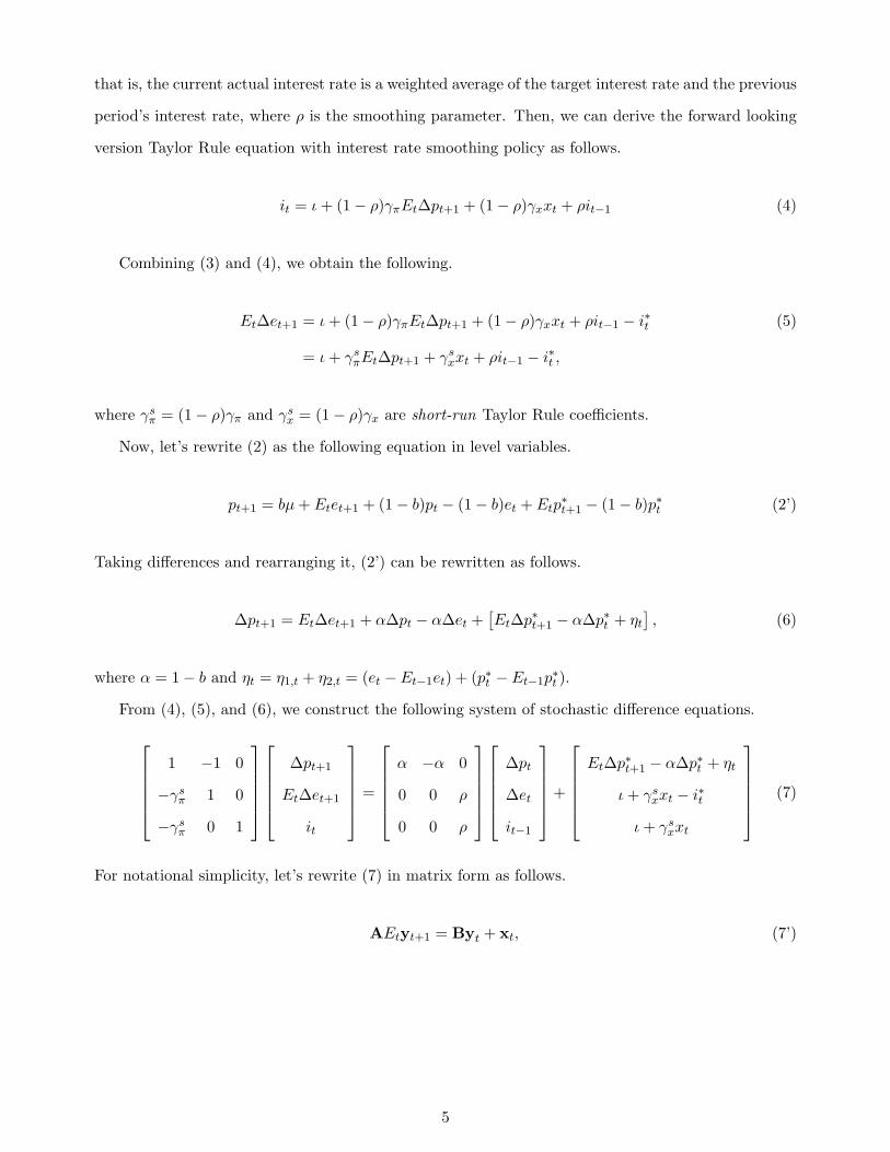
that is, the current actual interest rate is a weighted average of the target interest rate and the previous

period’s interest rate, where ρ is the smoothing parameter. Then, we can derive the forward looking

version Taylor Rule equation with interest rate smoothing policy as follows.

it = ι+ (1− ρ)γπEt∆pt+1 + (1− ρ)γxxt + ρit−1 (4)

Combining (3) and (4), we obtain the following.

Et∆et+1 = ι+ (1− ρ)γπEt∆pt+1 + (1− ρ)γxxt + ρit−1 − i∗t (5)

= ι+ γsπEt∆pt+1 + γs

xxt + ρit−1 − i∗t ,

where γsπ = (1− ρ)γπ and γs

x = (1− ρ)γx are short-run Taylor Rule coefficients.

Now, let’s rewrite (2) as the following equation in level variables.

pt+1 = bµ+ Etet+1 + (1− b)pt − (1− b)et + Etp∗t+1 − (1− b)p∗t (2’)

Taking differences and rearranging it, (2’) can be rewritten as follows.

∆pt+1 = Et∆et+1 + α∆pt − α∆et +[Et∆p∗t+1 − α∆p∗t + ηt

], (6)

where α = 1− b and ηt = η1,t + η2,t = (et − Et−1et) + (p∗t − Et−1p∗t ).

From (4), (5), and (6), we construct the following system of stochastic difference equations.

1 −1 0

−γsπ 1 0

−γsπ 0 1

∆pt+1

Et∆et+1

it

=

α −α 0

0 0 ρ

0 0 ρ

∆pt

∆et

it−1

+

Et∆p∗t+1 − α∆p∗t + ηt

ι+ γsxxt − i∗t

ι+ γsxxt

(7)

For notational simplicity, let’s rewrite (7) in matrix form as follows.

AEtyt+1 = Byt + xt, (7’)

5

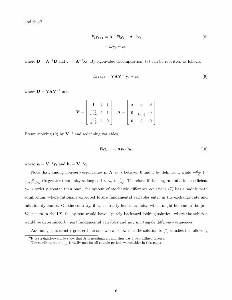
and thus6,

Etyt+1 = A−1Byt + A−1xt (8)

= Dyt + ct,

where D = A−1B and ct = A−1xt. By eigenvalue decomposition, (8) can be rewritten as follows.

Etyt+1 = VΛV−1yt + ct, (9)

where D = VΛV−1 and

V =

1 1 1

αγsπ

α−ρ 1 1αγs

πα−ρ 1 0

, Λ =

α 0 0

0 ρ1−γs

π0

0 0 0

Premultiplying (9) by V−1 and redefining variables,

Etzt+1 = Λzt+ht, (10)

where zt = V−1yt and ht = V−1ct.

Note that, among non-zero eigenvalues in Λ, α is between 0 and 1 by definition, while ρ1−γs

π(=

ρ1−(1−ρ)γπ

) is greater than unity as long as 1 < γπ <1

1−ρ . Therefore, if the long-run inflation coefficient

γπ is strictly greater than one7, the system of stochastic difference equations (7) has a saddle path

equilibrium, where rationally expected future fundamental variables enter in the exchange rate and

inflation dynamics. On the contrary, if γπ is strictly less than unity, which might be true in the pre-

Volker era in the US, the system would have a purely backward looking solution, where the solution

would be determined by past fundamental variables and any martingale difference sequences.

Assuming γπ is strictly greater than one, we can show that the solution to (7) satisfies the following6It is straightforward to show that A is nonsingular, and thus has a well-defined inverse.7The condition γπ < 1

1−ρis easily met for all sample periods we consider in this paper.

6

relation (see Appendix for the derivation).

∆et+1 = ι+αγs

π

α− ρ∆pt+1 −

αγsπ

α− ρ∆p∗t+1 +

αγsπ − (α− ρ)α− ρ

i∗t (11)

+γs

π(αγsπ − (α− ρ))

(α− ρ)ρ

∞∑j=0

(1− γs

π

ρ

)j

Etft+j+1 + ωt+1,

where,

ι =αγs

π − (α− ρ)(α− ρ)(γs

π − (1− ρ))ι,

Etft+j = −[Eti

∗t+j − Et∆p∗t+1+j

]+γs

x

γsπ

Etxt+j

= −Etr∗t+j +

γx

γπEtxt+j ,

ωt+1 =γs

π(αγsπ − (α− ρ))

(α− ρ)ρ

∞∑j=0

(1− γs

π

ρ

)j

(Et+1ft+j+1 − Etft+j+1)

+γs

π

α− ρηt+1 −

αγsπ − (α− ρ)α− ρ

υt+1,

and,

Etωt+1 = 0

Or, (11) can be rewritten with full parameter specification as follows.

∆et+1 = ι+αγπ(1− ρ)α− ρ

∆pt+1 −αγπ(1− ρ)α− ρ

∆p∗t+1 +αγπ(1− ρ)− (α− ρ)

α− ρi∗t (11’)

+γπ(1− ρ)(αγπ(1− ρ)− (α− ρ))

(α− ρ)ρ

∞∑j=0

(1− γπ(1− ρ)

ρ

)j

Etft+j+1 + ωt+1

Here, ft is a proxy variable that summarizes the fundamental variables such as foreign real interest

rates (r∗t ) and domestic output deviations.

Note that if γπ is strictly less than unity, the restriction in (11) may not be valid, since the system

would have a backward looking equilibrium rather than a saddle path equilibrium8. Put it differently,

exchange rate dynamics critically depends on the size of γπ. As mentioned in the introduction, however,

we have some supporting empirical evidence for such a requirement for the existence of a saddle path8If the system has a purely backward looking solution, the conventional structural Vector Autoregressive (SVAR)

estimation method may apply.

7

equilibrium, at least for the post-Volker era. So we believe that our specification would remain valid

for our purpose in this paper.

3 Estimation Methods

We discuss two estimation strategies here: a conventional univariate equation approach and the GMM

system method (Kim, Ogaki, and Yang, 2007).

3.1 Univariate Equation Approach

A univariate approach utilizes the equations (1) or (2). For instance, the persistence parameter α

in (1) can be consistently estimated by the conventional least squares method under the maintained

cointegrating relation assumption. Once we obtain the point estimate of α, the half-life of the real

exchange rate can be calculated by ln(.5)ln α . Similarly, the regression equation for the the convergence

parameter b can be constructed from (2) as follows.

∆pt+1 = b [µ− (pt − p∗t − et)] + ∆p∗t+1 + ∆et+1 + εt+1, (2”)

where εt+1 = ε1t+1 + ε2t+1 = (Et∆et+1 −∆et+1) + (Et∆p∗t+1 −∆p∗t+1) and Etεt+1 = 0.

3.2 GMM System Method

Our second estimation strategy combines the equation (11) with (1). The estimation of the equation

(11) is a challenging task, however, since it has an infinite sum of rationally expected discounted future

fundamental variables. Following Hansen and Sargent (1980, 1982), we linearly project Et(·) onto Ωt,

the econometrician’s information set at time t, which is a subset of It. Denoting Et(·) as such a linear

projection operator onto Ωt, we can rewrite (11) as follows.

∆et+1 = ι+αγs

π

α− ρ∆pt+1 −

αγsπ

α− ρ∆p∗t+1 +

αγsπ − (α− ρ)α− ρ

i∗t (12)

+γs

π(αγsπ − (α− ρ))

(α− ρ)ρ

∞∑j=0

(1− γs

π

ρ

)j

Etft+j+1 + ξt+1,

where

ξt+1 = ωt+1 +γs

π(αγsπ − (α− ρ))

(α− ρ)ρ

∞∑j=0

(1− γs

π

ρ

)j (Etft+j+1 − Etft+j+1

),

8

and

Etξt+1 = 0,

by the law of iterated projections.

Rather than choosing appropriate instrumental variables that are in Ωt, we simply assume Ωt =

ft, ft−1, ft−2, · · · . This assumption would be an innocent one under the stationarity assumption

of the fundamental variable, ft, and it can greatly lessen the burden in our GMM estimation by

significantly reducing the number of coefficients to be estimated.

Let’s assume, for now, that ft be a zero mean covariance stationary, linearly indeterministic stochas-

tic process so that it has the following Wold representation.

ft = c(L)νt, (13)

where νt = ft − Et−1ft and c(L) is square summable. Assuming that c(L) = 1 + c1L + c2L2 + · · · is

invertible, (13) can be rewritten as the following autoregressive representation.

b(L)ft = νt, (14)

where b(L) = c−1(L) = 1 − b1L − b2L2 − · · · . Linearly projecting

∑∞j=0

(1−γs

πρ

)jEtft+j+1 onto Ωt,

Hansen and Sargent (1980) show that the following relation holds.

∞∑j=0

δjEtft+j+1 = ψ(L)ft =

[1−

(δ−1b(δ)

)−1b(L)L−1

1− (δ−1L)−1

]ft, (15)

where δ = 1−γsπ

ρ .

For actual estimation, we assume that ft can be represented by a finite order AR(r) process9, that

is, b(L) = 1 −∑r

j=1 bjLj , where r < ∞. Then, it can be shown that the coefficients of ψ(L) can be

computed recursively (see Sargent 1987) as follows.

ψ0 = (1− δb1 − · · · − δrbr)−1

ψr = 09We can use conventional Akaike Information criteria or Bayesian Information criteria in order to choose the degree

of such autoregressive processes.

9

ψj−1 = δψj + δψ0bj ,

where j = 1, 2, · · · , r. Then, we obtain the following two orthogonality conditions.

∆et+1 = ι+αγs

π

α− ρ∆pt+1 −

αγsπ

α− ρ∆p∗t+1 +

αγsπ − (α− ρ)α− ρ

i∗t (16)

+γs

π(αγsπ − (α− ρ))

(α− ρ)ρ(ψ0ft + ψ1ft−1 + · · ·+ ψr−1ft−r+1) + ξt+1,

ft+1 = k + b1ft + b2ft−1 + · · ·+ brft−r+1 + νt+1, (17)

where k is a constant scalar1011, and Etνt+1 = 0.

Finally, the system method (GMM) estimation utilizes all aforementioned orthogonality conditions,

(2”), (16), and (17). That is, a GMM estimation can be implemented by the following 2(p + 2)

orthogonality conditions.

Ex1,t(st+1 − d− αst) = 0 (18)

Ex2,t−τ

∆et+1 − ι− αγsπ

α−ρ∆pt+1 + αγsπ

α−ρ∆p∗t+1 −αγs

π−(α−ρ)α−ρ i∗t

−γsπ(αγs

π−(α−ρ))(α−ρ)ρ (ψ0ft + ψ1ft−1 + · · ·+ ψr−1ft−r+1)

= 0 (19)

Ex2,t−τ (ft+1 − k − b1ft − b2ft−1 − · · · − brft−r+1) = 0, (20)

where x1,t = (1 st)′, x2,t = (1 ft)′, and τ = 0, 1, · · · , p1213.

3.3 Median Unbiased Estimator and Grid-t Confidence Intervals

We correct for the bias in our α estimates by a GMM version of the grid-t method proposed by

Hansen (1999) for the least squares estimator. It is straightforward to generate pseudo samples for

the orthogonality condition (20) by the conventional residual-based bootstrapping. However, there are

some complications in obtaining samples directly from (18) and (19), since p∗t is treated as a forcing

variable in our model. We deal with this problem as follows.

In order to generate pseudo samples for the orthogonality conditions (18) and (19), we denote pt

10Recall that Hansen and Sargent (1980) assume a zero-mean covariance stationary process. If the variable of interesthas a non-zero unconditional mean, we can either demean it prior to the estimation or include a constant but leave itscoefficient unconstrained. West (1989) showed that the further efficiency gain can be obtained by imposing additionalrestrictions on the deterministic term. However, the imposition of such an additional restriction is quite burdensome, sowe simply add a constant here.

11In actual estimations, we normalized (16) by multiplying (α − ρ) to each side in order to reduce nonlinearity.12p does not necessarily coincide with r.13In actual estimations, we use the aforementioned normalization again.

10

as the relative price index pt − p∗t . Then, (2”) and (16) can be rewritten as follows.

∆pt+1 = µ− b(pt − et) + ∆et+1 + εt+1

∆et+1 = ι+αγs

π

α− ρ∆pt+1 +

αγsπ − (α− ρ)α− ρ

i∗t

+γs

π(αγsπ − (α− ρ))

(α− ρ)ρ(ψ0ft + · · ·+ ψr−1ft−r+1) + ξt+1

Or, in matrix form,

∆pt+1

∆et+1

= C + S−1

−(1− α)

0

[pt − et] (21)

+ S−1

0

αγsπ−(α−ρ)α−ρ i∗t + γs

π(αγsπ−(α−ρ))

(α−ρ)ρ ·

(ψ0ft + · · ·+ ψr−1ft−r+1)

+ S−1

εt+1

ξt+1

,

where C is a vector of constants and S is[1 − 1

... − αγsπ

α−ρ 1].

Then, treating each grid point α ∈ [αmin, αmax] as a true value, we can generate pseudo samples of

∆pt+1 and ∆et+1 by the conventional bootstrapping14. The level variables pt and et are obtained by

numerical integration. It should be noted that all other parameters are treated as nuisance parameters

(η)15. Following Hansen (1999), we define the grid-t statistic at each grid point α ∈ [αmin, αmax] as

follows.

tn(α) =αGMM − α

se(αGMM), (22)

where se(αGMM) denotes the robust GMM standard error at the GMM estimate αGMM. Implementing

GMM estimations for B bootstrap iterations at each of N grid point of α, we obtain the (β quantile)

grid-t bootstrap quantile functions, q∗n,β(α) = q∗n,β(α, η(α)). Note that each function is evaluated at

each grid point α rather than at the point estimate16.

Finally, we define the 95% grid-t confidence interval as follows.

α ∈ R : q∗n,2.5%(α) ≤ tn(α) ≤ q∗n,97.5%(α), (23)14The historical data were used for the initial values and the foreign interest rate i∗t .15See Hansen (1999) for detailed explanations.16If they are evaluated at the point estimate, the quantile functions correspond to the Efron and Tibshirani’s (1993)

bootstrap-t quantile functions.

11

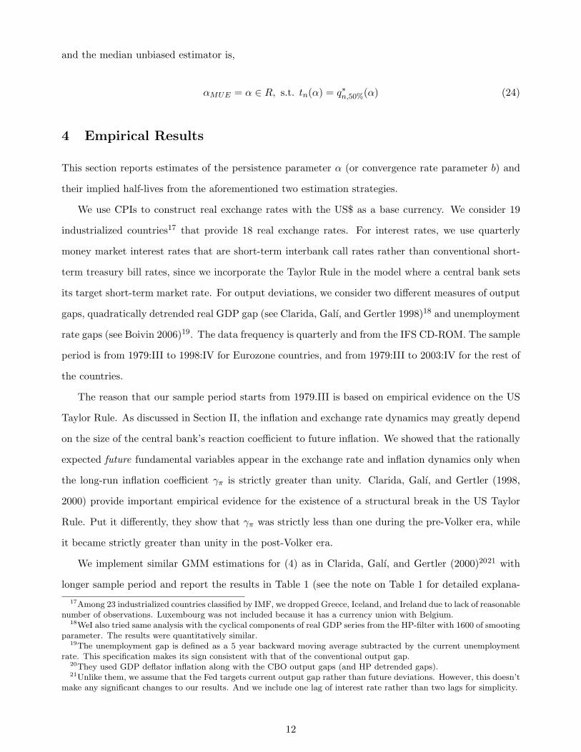
and the median unbiased estimator is,

αMUE = α ∈ R, s.t. tn(α) = q∗n,50%(α) (24)

4 Empirical Results

This section reports estimates of the persistence parameter α (or convergence rate parameter b) and

their implied half-lives from the aforementioned two estimation strategies.

We use CPIs to construct real exchange rates with the US$ as a base currency. We consider 19

industrialized countries17 that provide 18 real exchange rates. For interest rates, we use quarterly

money market interest rates that are short-term interbank call rates rather than conventional short-

term treasury bill rates, since we incorporate the Taylor Rule in the model where a central bank sets

its target short-term market rate. For output deviations, we consider two different measures of output

gaps, quadratically detrended real GDP gap (see Clarida, Galı, and Gertler 1998)18 and unemployment

rate gaps (see Boivin 2006)19. The data frequency is quarterly and from the IFS CD-ROM. The sample

period is from 1979:III to 1998:IV for Eurozone countries, and from 1979:III to 2003:IV for the rest of

the countries.

The reason that our sample period starts from 1979.III is based on empirical evidence on the US

Taylor Rule. As discussed in Section II, the inflation and exchange rate dynamics may greatly depend

on the size of the central bank’s reaction coefficient to future inflation. We showed that the rationally

expected future fundamental variables appear in the exchange rate and inflation dynamics only when

the long-run inflation coefficient γπ is strictly greater than unity. Clarida, Galı, and Gertler (1998,

2000) provide important empirical evidence for the existence of a structural break in the US Taylor

Rule. Put it differently, they show that γπ was strictly less than one during the pre-Volker era, while

it became strictly greater than unity in the post-Volker era.

We implement similar GMM estimations for (4) as in Clarida, Galı, and Gertler (2000)2021 with

longer sample period and report the results in Table 1 (see the note on Table 1 for detailed explana-17Among 23 industrialized countries classified by IMF, we dropped Greece, Iceland, and Ireland due to lack of reasonable

number of observations. Luxembourg was not included because it has a currency union with Belgium.18WeI also tried same analysis with the cyclical components of real GDP series from the HP-filter with 1600 of smooting

parameter. The results were quantitatively similar.19The unemployment gap is defined as a 5 year backward moving average subtracted by the current unemployment

rate. This specification makes its sign consistent with that of the conventional output gap.20They used GDP deflator inflation along with the CBO output gaps (and HP detrended gaps).21Unlike them, we assume that the Fed targets current output gap rather than future deviations. However, this doesn’t

make any significant changes to our results. And we include one lag of interest rate rather than two lags for simplicity.

12

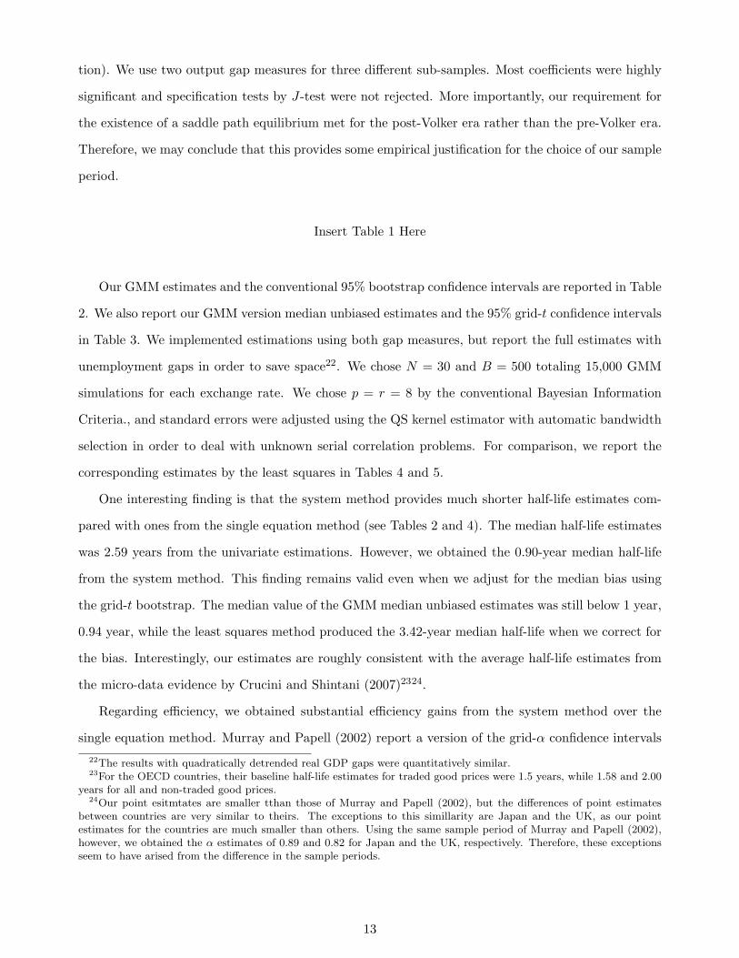
tion). We use two output gap measures for three different sub-samples. Most coefficients were highly

significant and specification tests by J-test were not rejected. More importantly, our requirement for

the existence of a saddle path equilibrium met for the post-Volker era rather than the pre-Volker era.

Therefore, we may conclude that this provides some empirical justification for the choice of our sample

period.

Insert Table 1 Here

Our GMM estimates and the conventional 95% bootstrap confidence intervals are reported in Table

2. We also report our GMM version median unbiased estimates and the 95% grid-t confidence intervals

in Table 3. We implemented estimations using both gap measures, but report the full estimates with

unemployment gaps in order to save space22. We chose N = 30 and B = 500 totaling 15,000 GMM

simulations for each exchange rate. We chose p = r = 8 by the conventional Bayesian Information

Criteria., and standard errors were adjusted using the QS kernel estimator with automatic bandwidth

selection in order to deal with unknown serial correlation problems. For comparison, we report the

corresponding estimates by the least squares in Tables 4 and 5.

One interesting finding is that the system method provides much shorter half-life estimates com-

pared with ones from the single equation method (see Tables 2 and 4). The median half-life estimates

was 2.59 years from the univariate estimations. However, we obtained the 0.90-year median half-life

from the system method. This finding remains valid even when we adjust for the median bias using

the grid-t bootstrap. The median value of the GMM median unbiased estimates was still below 1 year,

0.94 year, while the least squares method produced the 3.42-year median half-life when we correct for

the bias. Interestingly, our estimates are roughly consistent with the average half-life estimates from

the micro-data evidence by Crucini and Shintani (2007)2324.

Regarding efficiency, we obtained substantial efficiency gains from the system method over the

single equation method. Murray and Papell (2002) report a version of the grid-α confidence intervals22The results with quadratically detrended real GDP gaps were quantitatively similar.23For the OECD countries, their baseline half-life estimates for traded good prices were 1.5 years, while 1.58 and 2.00

years for all and non-traded good prices.24Our point esitmtates are smaller tthan those of Murray and Papell (2002), but the differences of point estimates

between countries are very similar to theirs. The exceptions to this simillarity are Japan and the UK, as our pointestimates for the countries are much smaller than others. Using the same sample period of Murray and Papell (2002),however, we obtained the α estimates of 0.89 and 0.82 for Japan and the UK, respectively. Therefore, these exceptionsseem to have arised from the difference in the sample periods.

13

(Hansen, 1999)25 of which upper limits of their half-life estimates are infinity for every exchange rates

they consider. Based on such results, they conclude that single equation methods may provide virtually

no useful information due to wide confidence intervals.

Our grid-t confidence intervals from the single equation method were consistent with such a view

(see Table 5). The upper limits are infinity for most real exchange rates. However, when we implement

estimations by the system method, the standard errors were reduced significantly, and our 95% GMM

version grid-t confidence intervals were very compact. Our results can be also considered as great

improvement over Kim, Ogaki, and Yang (2007) who acquired limited success in efficiency gains.

Insert Table 2 Here

Insert Table 3 Here

Insert Table 4 Here

Insert Table 5 Here

5 Conclusion

In this paper, we developed a system method that combines the Taylor rule and a standard exchange

rate model, and estimated the half-lives of the real exchange rates of 18 developed countries against

the U.S.

We used two types of nonparametric bootstrap methods in order to construct confidence inter-

vals: the standard bootstrap and Hansen’s (1999) grid bootstrap. The standard bootstrap evaluates

bootstrap quantiles at the point estimate of the AR(1) coefficient, which implicitly assumes that the

bootstrap quantile functions are constant functions. This assumption does not hold for the AR model,

and Hansen’s grid bootstrap method that avoids this assumption has better coverage properties. In25Their confidence intervals are constructed following Andrews (1993) and Andrews and Chen (1994), which are

identical to the Hansen’s (1999) grid-α confidence intervals if we assume that the errors are drawn from the empiricaldistribution rather than the i.i.d. normal distribution.

14

our applications, we often obtain very different confidence intervals for these two methods. Therefore,

the violation of the assumption is deemed quantitatively important..

When we use the grid bootstrap method, most of the (approximately) median unbiased estimates

from the single equation method fall in the range of 3 to 5 years with wide confidence intervals that

extend to the positive infinity. In contrast, the system method yields median unbiased estimates that

are typically substantially shorter than 3 years with much sharper confidence intervals most of which

range from 1 to 5 years.

These results indicate that monetary variables from the exchange rate model based on the Taylor

rule provide useful information about the half-lives of the real exchange rates. The estimators from

the system method are much sharper in the sense that confidence intervals are much narrower than

those from a single equation method. Approximate median unbiased estimates of the half-lives are

typically about one year, which is much more reasonable than consensus “3-5 years” from single

equation methods especially given recent empirical literature on price adjustments such as Bills and

Klenow (2005) that find frequent price adjustments.

15

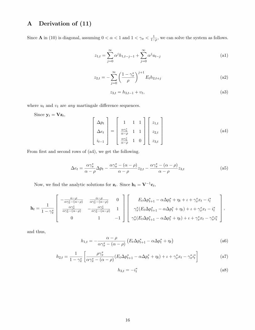
A Derivation of (11)

Since Λ in (10) is diagonal, assuming 0 < α < 1 and 1 < γπ <1

1−ρ , we can solve the system as follows.

z1,t =∞∑

j=0

αjh1,t−j−1 +∞∑

j=0

αjut−j (a1)

z2,t = −∞∑

j=0

(1− γs

π

ρ

)j+1

Eth2,t+j (a2)

z3,t = h3,t−1 + υt, (a3)

where ut and υt are any martingale difference sequences.

Since yt = Vzt, ∆pt

∆et

it−1

=

1 1 1

αγsπ

α−ρ 1 1αγs

πα−ρ 1 0

z1,t

z2,t

z3,t

(a4)

From first and second rows of (a4), we get the following.

∆et =αγs

π

α− ρ∆pt −

αγsπ − (α− ρ)α− ρ

z2,t −αγs

π − (α− ρ)α− ρ

z3,t (a5)

Now, we find the analytic solutions for zt. Since ht = V−1ct,

ht =1

1− γsπ

− α−ρ

αγsπ−(α−ρ)

α−ραγs

π−(α−ρ) 0αγs

παγs

π−(α−ρ) − αγsπ

αγsπ−(α−ρ) 1

0 1 −1

Et∆p∗t+1 − α∆p∗t + ηt + ι+ γsxxt − i∗t

γsπ(Et∆p∗t+1 − α∆p∗t + ηt) + ι+ γs

xxt − i∗t

γsπ(Et∆p∗t+1 − α∆p∗t + ηt) + ι+ γs

xxt − γsπi∗t

,

and thus,

h1,t = − α− ρ

αγsπ − (α− ρ)

(Et∆p∗t+1 − α∆p∗t + ηt

)(a6)

h2,t =1

1− γsπ

[ργs

π

αγsπ − (α− ρ)

(Et∆p∗t+1 − α∆p∗t + ηt) + ι+ γsxxt − γs

πi∗t

](a7)

h3,t = −i∗t (a8)

16

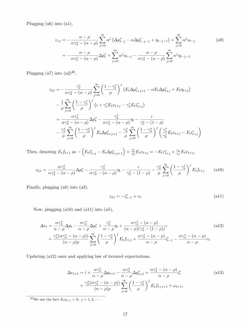
Plugging (a6) into (a1),

z1,t = − α− ρ

αγsπ − (α− ρ)

∞∑j=0

αj(∆p∗t−j − α∆p∗t−j−1 + ηt−j−1

)+

∞∑j=0

αjut−j (a9)

= − α− ρ

αγsπ − (α− ρ)

∆p∗t +∞∑

j=0

αjut−j −α− ρ

αγsπ − (α− ρ)

∞∑j=0

αjηt−j−1

Plugging (a7) into (a2)26,

z2,t = − γsπ

αγsπ − (α− ρ)

∞∑j=0

(1− γs

π

ρ

)j (Et∆p∗t+j+1 − αEt∆p∗t+j + Etηt+j

)− 1ρ

∞∑j=0

(1− γs

π

ρ

)j (ι+ γs

xEtxt+j − γsπEti

∗t+j

)=

αγsπ

αγsπ − (α− ρ)

∆p∗t −γs

π

αγsπ − (α− ρ)

ηt −ι

γsπ − (1− ρ)

− γsπ

ρ

∞∑j=0

(1− γs

π

ρ

)j

Et∆p∗t+j+1 −γs

π

ρ

∞∑j=0

(1− γs

π

ρ

)j (γs

x

γsπ

Etxt+j − Eti∗t+j

)

Then, denoting Etft+j as −(Eti

∗t+j − Et∆p∗t+j+1

)+ γs

xγs

πEtxt+j = −Etr

∗t+j + γx

γπEtxt+j ,

z2,t =αγs

π

αγsπ − (α− ρ)

∆p∗t −γs

π

αγsπ − (α− ρ)

ηt −ι

γsπ − (1− ρ)

− γsπ

ρ

∞∑j=0

(1− γs

π

ρ

)j

Etft+j (a10)

Finally, plugging (a8) into (a3),

z3,t = −i∗t−1 + υt (a11)

Now, plugging (a10) and (a11) into (a5),

∆et =αγs

π

α− ρ∆pt −

αγsπ

α− ρ∆p∗t +

γsπ

α− ρηt +

αγsπ − (α− ρ)

(α− ρ)(γsπ − (1− ρ))

ι (a12)

+γs

π(αγsπ − (α− ρ))

(α− ρ)ρ

∞∑j=0

(1− γs

π

ρ

)j

Etft+j +αγs

π − (α− ρ)α− ρ

i∗t−1 −αγs

π − (α− ρ)α− ρ

υt

Updating (a12) once and applying law of iterated expectations,

∆et+1 = ι+αγs

π

α− ρ∆pt+1 −

αγsπ

α− ρ∆p∗t+1 +

αγsπ − (α− ρ)α− ρ

i∗t (a13)

+γs

π(αγsπ − (α− ρ))

(α− ρ)ρ

∞∑j=0

(1− γs

π

ρ

)j

Etft+j+1 + ωt+1,

26We use the fact Etηt+j = 0, j = 1, 2, · · · .

17

where

ι =αγs

π − (α− ρ)(α− ρ)(γs

π − (1− ρ))ι,

ωt+1 =γs

π(αγsπ − (α− ρ))

(α− ρ)ρ

∞∑j=0

(1− γs

π

ρ

)j

(Et+1ft+j+1 − Etft+j+1)

+γs

π

α− ρηt+1 −

αγsπ − (α− ρ)α− ρ

υt+1,

and,

Etωt+1 = 0

18

References

Andrews, D. W. K. (1993): “Exactly Median-Unbiased Estimation of First Order Autoregres-

sive/Unit Root Models,” Econometrica, 61, 139–165.

Andrews, D. W. K., and H.-Y. Chen (1994): “Approximately Median-Unbiased Estimation of

Autoregressive Models,” Journal of Business and Economic Statistics, 12, 187–204.

Bils, M., and P. J. Klenow (2005): “Some Evidence on the Importance of Sticky Prices,” Journal

of Political Economy, 112, 947–985.

Boivin, J. (2006): “Has US Monetary Policy Changed? Evidence from Drifting Coefficients and Real

Time Data,” Journal of Money, Credit, and Banking, 38, 1149–1173.

Broda, C., and D. E. Weinstein (2007): “Understanding International Price Differences Using

Barcode Data,” mimeo.

Chen, S.-S., and C. Engel (2005): “Does ’Aggregation Bias” Explain the PPP Puzzle?,” Pacific

Economic Review, 10, 49–72.

Clarida, R., J. Gali, and M. Gertler (1998): “Monetary Policy Rules in Practice: Some Inter-

national Evidence,” European Economic Review, 42, 1033–1067.

(2000): “Monetary Policy Rules and Macroeconomic Stability: Evidence and Some Theory,”

Quarterly Journal of Economics, 115, 147–180.

Crucini, M. J., , and M. Shintani (2007): “Persistence in Law-of-One-Price Deviations: Evidence

from Micro-Data,” Journal of Monetary Economics.

Efron, B., and R. J. Tibshirani (1993): An Introduction to the Bootstrap. Chapman and Hall/CRC,

London, UK.

Engel, C., and K. D. West (2006): “Taylor Rules and the Deutschmark-Dollar Exchange Rate,”

Journal of Money, Credit, and Banking, 38, 1175–1194.

Hansen, B. E. (1999): “The Grid Bootstrap and the Autoregressive Model,” Review of Economics

and Statistics, 81, 594–607.

Hansen, L. P. (1982): “Large Sample Properties of Generalized Method of Moments Estimators,”

Econometrica, 50, 1029–1054.

19

Hansen, L. P., and T. J. Sargent (1980): “Formulating and Estimating Dynamic Linear Rational

Expectations Models,” Journal of Economic Dynamics and Control, 2, 7–46.

(1981): “A Note on Wiener-Kolmogorov Prediction Formulas for Rational Expectations

Models,” Research Department Staff Report 69, Federal Reserve Bank of Minneapolis, Minneapolis,

MN.

(1982): “Instrumental Variables Procedures for Estimating Linear Rational Expectations

Models,” Journal of Monetary Economics, 9, 263–296.

Imbs, J., H. Mumtaz, M. O. Ravn, and H. Rey (2005): “PPP Strikes Back: Aggregation and the

Real Exchange Rates,” Quarterly Journal of Economics, 120, 1–43.

Kilian, L., and T. Zha (2002): “Quantifying the Uncertainty about the Half-Life of Deviations from

PPP,” Journal of Applied Econometrics, 17, 107–125.

Kim, H. (2006): “Essays on Exchange Rate Models under a Taylor Rule Type Monetary Policy,”

Ph.D. Dissertation, Ohio State University.

Kim, J. (2005): “Convergence Rates to PPP for Traded and Non-Traded Goods: A Structural Error

Correction Model Approach,” Journal of Business and Economic Statistics, 23, 76–86.

Kim, J., and M. Ogaki (2004): “Purchasing Power Parity for Traded and Non-Traded Goods: A

Structural Error Correction Model Approach,” Monetary and Economic Studies, 22, 1–26.

Kim, J., M. Ogaki, and M.-S. Yang (2007): “Structural Error Correction Models: A System

Method for Linear Rational Expectations Models and an Application to an Exchange Rate Model,”

Journal of Money, Credit, and Banking, 39.

Mark, N. C. (2001): International Macroeconomics and Finance: Theory and Econometric Methods.

Blackwell Publishers, Oxford, UK.

(2005): “Changing Monetary Policy Rules, Learning, and Real Exchange Rate Dynamics,”

National Bureau of Economic Research Working Paper No. 11061.

Molodtsova, T., A. Nikolsko-Rzhevskyy, and D. H. Papell (2007): “Taylor Rule with Real-

Time Data: A Tale of Two Countries and One Exchange Rate,” Manuscript, University of Houston.

20

Molodtsova, T., and D. H. Papell (2007): “Out-of-Sample Exchange Rate Predictability with

Taylor Rule Fundamentals,” Manuscript, University of Houston.

Murray, C. J., and D. H. Papell (2002): “The Purchasing Power Parity Persistence Paradigm,”

Journal of International Economics, 56, 1–19.

(2005): “Do Panels Help Solve the Purchasing Power Parity Puzzle?,” Journal of Business

and Economic Statistics, 23, 410–415.

Mussa, M. (1982): “A Model of Exchange Rate Dynamics,” Journal of Political Economy, 90, 74–104.

Ogaki, M. (1993): “Generalized Method of Moments: Econometric Applications,” in Handbook of

Statistics, Vol.II, ed. by G. S. Maddala, C. R. Rao, and H. D. Vinod, pp. 455–488, Amsterdam.

North-Holland.

Rogoff, K. (1996): “The Purchasing Power Parity Puzzle,” Journal of Economic Literature, 34,

647–668.

Sargent, T. J. (1987): Macroeconomic Theory. Academic Press, New York, second edn.

Stock, J. H., and M. W. Watson (1993): “A Simple Estimator of Cointegrating Vectors in Higher

Order Integrated Systems,” Econometrica, 61, 783–820.

West, K. D. (1987): “A Specification Test for Speculative Bubbles,” Quarterly Journal of Economics,

12, 553–580.

(1989): “Estimation of Linear Rational Expectations Models, In the Presence of Deterministic

Terms,” Journal of Monetary Economics, 24, 437–442.

21

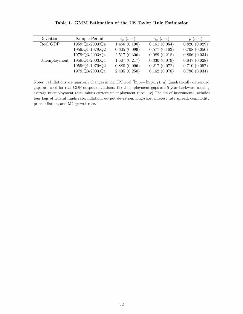
Table 1. GMM Estimation of the US Taylor Rule Estimation

Deviation Sample Period γπ (s.e.) γx (s.e.) ρ (s.e.)Real GDP 1959:Q1-2003:Q4 1.466 (0.190) 0.161 (0.054) 0.820 (0.029)

1959:Q1-1979:Q2 0.605 (0.099) 0.577 (0.183) 0.708 (0.056)1979:Q3-2003:Q4 2.517 (0.306) 0.089 (0.218) 0.806 (0.034)

Unemployment 1959:Q1-2003:Q4 1.507 (0.217) 0.330 (0.079) 0.847 (0.028)1959:Q1-1979:Q2 0.880 (0.096) 0.217 (0.072) 0.710 (0.057)1979:Q3-2003:Q4 2.435 (0.250) 0.162 (0.078) 0.796 (0.034)

Notes: i) Inflations are quarterly changes in log CPI level (ln pt− ln pt−1). ii) Quadratically detrendedgaps are used for real GDP output deviations. iii) Unemployment gaps are 5 year backward movingaverage unemployment rates minus current unemployment rates. iv) The set of instruments includesfour lags of federal funds rate, inflation, output deviation, long-short interest rate spread, commodityprice inflation, and M2 growth rate.

22

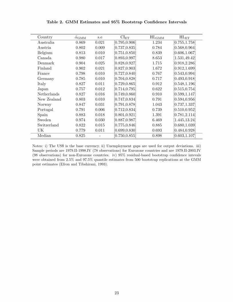
Table 2. GMM Estimates and 95% Bootstrap Confidence Intervals

Country αGMM s.e CIET HLGMM HLET

Australia 0.869 0.021 [0.795,0.906] 1.234 [0.755,1.758]Austria 0.802 0.009 [0.737,0.835] 0.784 [0.568,0.964]Belgium 0.813 0.010 [0.751,0.850] 0.839 [0.606,1.067]Canada 0.980 0.017 [0.893,0.997] 8.653 [1.531,49.42]Denmark 0.904 0.025 [0.828,0.927] 1.715 [0.918,2.286]Finland 0.902 0.021 [0.827,0.903] 1.672 [0.912,1.699]France 0.798 0.010 [0.727,0.840] 0.767 [0.543,0.994]Germany 0.785 0.010 [0.704,0.828] 0.717 [0.493,0.918]Italy 0.827 0.011 [0.729,0.865] 0.912 [0.548,1.196]Japan 0.757 0.012 [0.714,0.795] 0.622 [0.515,0.754]Netherlands 0.827 0.016 [0.749,0.860] 0.910 [0.599,1.147]New Zealand 0.803 0.010 [0.747,0.834] 0.791 [0.594,0.956]Norway 0.847 0.031 [0.791,0.878] 1.043 [0.737,1.337]Portugal 0.791 0.006 [0.712,0.834] 0.739 [0.510,0.952]Spain 0.883 0.018 [0.801,0.921] 1.391 [0.781,2.114]Sweden 0.974 0.030 [0.887,0.987] 6.469 [1.445,13.24]Switzerland 0.822 0.015 [0.775,0.846] 0.885 [0.680,1.039]UK 0.779 0.011 [0.699,0.830] 0.693 [0.484,0.928]Median 0.825 - [0.750,0.855] 0.898 [0.603,1.107]

Notes: i) The US$ is the base currency. ii) Unemployment gaps are used for output deviations. iii)Sample periods are 1979.II-1998.IV (78 observations) for Eurozone countries and are 1979.II-2003.IV(98 observations) for non-Eurozone countries. iv) 95% residual-based bootstrap confidence intevalswere obtained from 2.5% and 97.5% quantile estimates from 500 bootstrap replications at the GMMpoint estimates (Efron and Tibshirani, 1993).

23

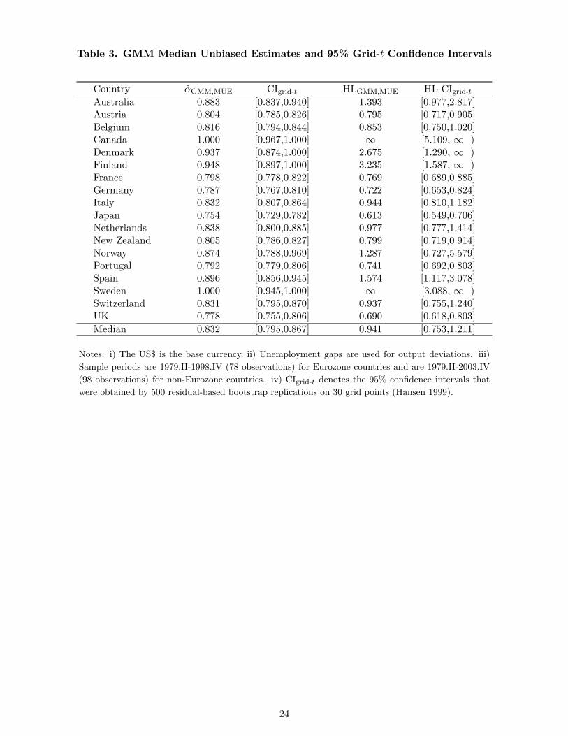
Table 3. GMM Median Unbiased Estimates and 95% Grid-t Confidence Intervals

Country αGMM,MUE CIgrid-t HLGMM,MUE HL CIgrid-t

Australia 0.883 [0.837,0.940] 1.393 [0.977,2.817]Austria 0.804 [0.785,0.826] 0.795 [0.717,0.905]Belgium 0.816 [0.794,0.844] 0.853 [0.750,1.020]Canada 1.000 [0.967,1.000] ∞ [5.109, ∞ )Denmark 0.937 [0.874,1.000] 2.675 [1.290, ∞ )Finland 0.948 [0.897,1.000] 3.235 [1.587, ∞ )France 0.798 [0.778,0.822] 0.769 [0.689,0.885]Germany 0.787 [0.767,0.810] 0.722 [0.653,0.824]Italy 0.832 [0.807,0.864] 0.944 [0.810,1.182]Japan 0.754 [0.729,0.782] 0.613 [0.549,0.706]Netherlands 0.838 [0.800,0.885] 0.977 [0.777,1.414]New Zealand 0.805 [0.786,0.827] 0.799 [0.719,0.914]Norway 0.874 [0.788,0.969] 1.287 [0.727,5.579]Portugal 0.792 [0.779,0.806] 0.741 [0.692,0.803]Spain 0.896 [0.856,0.945] 1.574 [1.117,3.078]Sweden 1.000 [0.945,1.000] ∞ [3.088, ∞ )Switzerland 0.831 [0.795,0.870] 0.937 [0.755,1.240]UK 0.778 [0.755,0.806] 0.690 [0.618,0.803]Median 0.832 [0.795,0.867] 0.941 [0.753,1.211]

Notes: i) The US$ is the base currency. ii) Unemployment gaps are used for output deviations. iii)Sample periods are 1979.II-1998.IV (78 observations) for Eurozone countries and are 1979.II-2003.IV(98 observations) for non-Eurozone countries. iv) CIgrid-t denotes the 95% confidence intervals thatwere obtained by 500 residual-based bootstrap replications on 30 grid points (Hansen 1999).

24

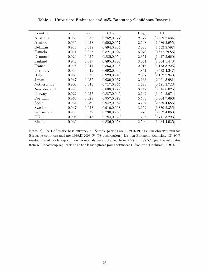
Table 4. Univariate Estimates and 95% Bootstrap Confidence Intervals

Country αLS s.e. CIET HLLS HLET

Australia 0.935 0.033 [0.752,0.977] 2.572 [0.609,7.534]Austria 0.936 0.038 [0.902,0.957] 2.608 [1.686,3.955]Belgium 0.918 0.038 [0.894,0.935] 2.038 [1.552,2.597]Canada 0.971 0.023 [0.821,0.994] 5.970 [0.877,29.85]Denmark 0.929 0.035 [0.885,0.954] 2.351 [1.417,3.660]Finland 0.945 0.037 [0.895,0.969] 3.051 [1.564,5.473]France 0.918 0.041 [0.863,0.948] 2.015 [1.173,3.225]Germany 0.910 0.042 [0.693,0.960] 1.841 [0.473,4.247]Italy 0.936 0.039 [0.923,0.943] 2.607 [2.152,2.943]Japan 0.947 0.032 [0.930,0.957] 3.188 [2.391,3.981]Netherlands 0.902 0.043 [0.717,0.955] 1.688 [0.521,3.723]New Zealand 0.946 0.017 [0.808,0.979] 3.142 [0.815,8.026]Norway 0.922 0.037 [0.887,0.945] 2.142 [1.451,3.074]Portugal 0.969 0.029 [0.957,0.978] 5.503 [3.964,7.696]Spain 0.954 0.030 [0.942,0.964] 3.704 [2.889,4.686]Sweden 0.947 0.028 [0.910,0.968] 3.152 [1.830,5.355]Switzerland 0.916 0.039 [0.730,0.958] 1.976 [0.552,4.068]UK 0.908 0.043 [0.784,0.949] 1.796 [0.711,3.293]Median 0.936 - [0.886,0.958] 2.590 [1.434,4.025]

Notes: i) The US$ is the base currency. ii) Sample periods are 1979.II-1998.IV (78 observations) forEurozone countries and are 1979.II-2003.IV (98 observations) for non-Eurozone countries. iii) 95%residual-based bootstrap confidence intevals were obtained from 2.5% and 97.5% quantile estimatesfrom 500 bootstrap replications at the least squares point estimates (Efron and Tibshirani, 1993).

25

Table 5. Univariate Median Unbiased Estimates and Grid-t Confidence Intervals

Country αLS,MUE CIgrid-t HLLS,MUE HL CIgrid-t

Australia 0.972 [0.891,1.000] 6.173 [1.494, ∞ )Austria 0.945 [0.866,1.000] 3.087 [1.205, ∞ )Belgium 0.924 [0.847,1.000] 2.203 [1.045, ∞ )Canada 1.000 [0.946,1.000] ∞ [3.122, ∞ )Denmark 0.942 [0.866,1.000] 2.886 [1.200, ∞ )Finland 0.959 [0.883,1.000] 4.107 [1.390, ∞ )France 0.931 [0.847,1.000] 2.432 [1.044, ∞ )Germany 0.950 [0.852,1.000] 3.349 [1.078, ∞ )Italy 0.943 [0.859,1.000] 2.932 [1.138, ∞ )Japan 0.952 [0.886,1.000] 3.511 [1.428, ∞ )Netherlands 0.936 [0.839,1.000] 2.619 [0.990, ∞ )New Zealand 0.959 [0.923,0.997] 4.089 [2.174,61.29]Norway 0.934 [0.851,1.000] 2.529 [1.073, ∞ )Portugal 0.975 [0.913,1.000] 6.765 [1.904, ∞ )Spain 0.959 [0.898,1.000] 4.129 [1.604, ∞ )Sweden 0.959 [0.891,1.000] 4.089 [1.497, ∞ )Switzerland 0.951 [0.862,1.000] 3.481 [1.168, ∞ )UK 0.932 [0.845,1.000] 2.442 [1.028, ∞ )Median 0.951 [0.866,1.000] 3.415 [1.203, ∞ )

Notes: i) The US$ is the base currency. ii) Sample periods are 1979.II-1998.IV (78 observations) forEurozone countries and are 1979.II-2003.IV (98 observations) for non-Eurozone countries. iii) CIgrid-t

denotes the 95% confidence intervals that were obtained by 500 residual-based bootstrap replicationson 30 grid points (Hansen, 1999).

26